Inversely Learning Transferable Rewards via Abstracted States

Abstract

Inverse reinforcement learning (IRL) has progressed significantly toward accurately learning the underlying rewards in both discrete and continuous domains from behavior data. The next advance is to learn intrinsic preferences in ways that produce useful behavior in settings or tasks that are different but aligned with the observed ones. In the context of robotic applications, this could help integrate robots into processing lines involving new tasks (with shared intrinsic preferences) without programming from scratch. We introduce a method to inversely learn an abstract reward function from behavior trajectories in two or more differing instances of a domain. The abstract reward function is then used to learn task behavior in another separate instance of the domain. The latter step offers evidence of its transferability and validates its correctness. We evaluate the method on trajectories of tasks from multiple domains in OpenAI’s Gym testbed and AssistiveGym and show that the learned abstract reward functions can successfully learn task behaviors in instances of the respective domains, which have not been seen previously.

1 Introduction

The objective of inverse reinforcement learning (IRL) is one of abductive reasoning: to infer the reward function that best explains the observed trajectories. This is challenging because the available data is often sparse, which admits many potential solutions (some degenerate), and the learned reward functions may not generalize for use in target instances that could be slightly different. Despite these challenges, significant progress has been made in the last decade toward learning the underlying reward functions in both discrete and continuous domains, which are accurate (in yielding the observed behavior) and parsimonious (Arora and Doshi, 2021). A key advance in IRL next is to learn reward functions that represent intrinsic preferences, which become relevant in aligned task instances not seen previously. This contributes to the transferability of the learned rewards – an important characteristic of a general solution.

In this paper, we introduce a new method that generalizes IRL to previously unseen tasks but which exhibit commonality with the observed ones in terms of shared core or intrinsic preferences. Abstractions offer a powerful representation for generalization (Allen et al., 2021), and so we introduce the concept of an abstract reward function. To illustrate, consider the Ant domain from OpenAI Gymnasium (Schulman et al., 2016) and two Ant environments with differing pairs of disabled legs as the source environments and an Ant environment with another pair of disabled legs as the target. As the source and target ants have different disabled legs, the marginal state distributions of the sources are different from the target’s, which makes it difficult to transfer a learned reward function. However, if we focus on the ant’s torso instead of its legs, the marginal state distribution of the torso remains mostly the same across both the sources and the target environment. So, learning a reward function based on the torso, which is the abstraction, allows the function to be transferred across any disabled leg. Our method utilizes observed behavior data from two or more differing instances of a task domain as input to a variational autoencoder (VAE). A single encoder is coupled with multiple decoders, one for each source instance, to reconstruct the instance trajectories. We show how the common latent variable(s) of this distinct VAE model can be interpreted and shaped as an abstract reward function that governs the input task behaviors. Note that two or more aligned task behaviors are needed to learn the shared intrinsic preferences to perform the tasks.

We evaluate our method for transferable IRL, labeled TraIRL, on multiple benchmarks: OpenAI Gym domains (Schulman et al., 2016) and the robotic AssistiveGym (Erickson et al., 2019). We utilize trajectories from two differing instances in each domain as input to the VAE and show how the inversely learned abstract reward function can help successfully learn the correct behavior in a third aligned instance of the domain. These results strongly indicate that we may learn abstract reward functions via IRL that offer a level of generalizability not presented previously in the literature.

2 Related Work

Extant transfer learning for IRL struggles with mismatches in environment dynamics, which limits reward transferability. Tanwani and Billard (2013) introduce an approach to learn diverse strategies from multiple experts, focusing on shared knowledge. However, it assumes unchanged dynamics between experts, which limits its applicability to dynamic environments. I2L (Gangwani and Peng, 2020) is designed for state-only imitation learning and addresses transition dynamics mismatches by using a prioritized trajectory buffer and optimizing a lower bound on the expert’s state-action visitation distribution. While empirically effective, it lacks theoretical guarantees on reward transferability and does not formally justify how the learned reward generalizes across different dynamics. Viano et al. (2024) analyzes MCE-IRL under transition dynamics mismatch, deriving necessary and sufficient conditions for its transferability and providing a tight bound on performance degradation. It proposes a robust MCE-IRL algorithm but struggles with generalization under action space shifts due to its reliance on matching state-action occupancy measures.

Rewards learned by adversarial IRL and IL methods may not transfer across environments. AIRL (Fu et al., 2018), $f$-MAX (Ghasemipour et al., 2020) and $f$-IRL (Ni et al., 2021) claim that their learned reward functions generalize to unseen or dynamically different environments. But, these claims are not supported by explicit structural frameworks or theoretical guarantees, leaving the transferability questionable. Furthermore, the learned rewards are tied to specific expert policy trajectories, preventing their use in training new policies from scratch. In contrast, IQ-Learn (Garg et al., 2021) is non-adversarial and learns soft Q-functions from expert data, which offers improved stability and efficiency. However, its reliance on action-dependent Q-functions limits generalization to state-only reward functions.

Reward identification or identifiability may not be sufficient for learning a transferable reward function, as it focuses on recovery only of the true reward function from expert demonstrations. Cao et al. (2024) mitigates reward ambiguity using an entropy-regularized framework. It relies on multiple optimal policies under varying dynamics, but the method is not suitable for scenarios that do not have such policies and does not focus on transferability. Rolland et al. (2024) presents a reward identification approach for discrete state-action spaces, utilizing variations across environments. However, the method struggles with continuous states and prioritizes identifiability over transferability. Kim et al. (2021) formalize reward identifiability in deterministic MDPs using the maximum entropy objective, and provide conditions for identifiability. But, the work does not address the challenge of creating transferable reward representations.

3 Background

We briefly review maximum causal entropy IRL (Ziebart et al., 2010) as it informs our method. The entropy-regularized Markov decision process (MDP) is characterized by the tuple $(\mathcal{S},\mathcal{A},\mathcal{T},r,\gamma,\rho_{0})$. Here, $\mathcal{S}$ and $\mathcal{A}$ denote the state and action spaces, respectively, while $\gamma\in(0,1)$ is the discount factor. In the standard RL context, the dynamics modeled by the transition distribution $T(s^{\prime}|a,s)$, the initial state distribution $\rho_{0}(s)$, and the reward function $r(s,a)$ are unknown, and can only be determined through interaction with the environment. Optimal policy $\pi$ under the maximum entropy framework maximizes the objective

$$\pi^{*}=\arg\max_{\pi}\mathbb{E}_{\tau\sim\pi}\left[\sum_{t=0}^{T}\gamma^{t}(r(s_{t},a_{t})+H(\pi(\cdot|s_{t})))\right],$$

where $\tau=(s_{0},a_{0},...,s_{T},a_{T})$ denotes a sequence of states and actions induced by the policy and transition function, and $H(\pi(\cdot|s))$ is the entropy of the action distribution from policy $\pi$ for state $s$.

Another IRL method, $f$-IRL (Ni et al., 2021), integrates $f$-divergence to improve scalability and robustness, which we utilize in our method. $f$-IRL relies on a generator-discriminator schema to recover a stationary reward function by matching the expert’s state marginal distribution (also called state density or occupancy distribution) – an approach that builds and improves on the state marginal matching (SMM) algorithm (Lee et al., 2019). Unlike traditional SMM, which focuses on implicitly matching state distributions, $f$-IRL explicitly derives the stationary reward function from the expert state density. We rely on a variant of $f$-IRL that minimizes the 1-Wasserstein distance between the state marginals, as this distance is an integral probability metric:

$$\mathcal{L}_{\mathcal{F}}({\bm{\theta}})=\mathcal{D}_{\mathcal{F}}(\rho_{E}||\rho_{\bm{\theta}})=W_{1}(\rho_{E}(s)\,,\,\rho_{\bm{\theta}}(s)).$$ (1)

where $D_{\mathcal{F}}$ is a divergence measure between distributions, $W_{1}$ is the 1-Wasserstein distance, $\rho_{E}$ and $\rho_{\bm{\theta}}$ denote the state densities of the expert and the soft-optimal learner under the reward function $r_{\bm{\theta}}$, respectively.

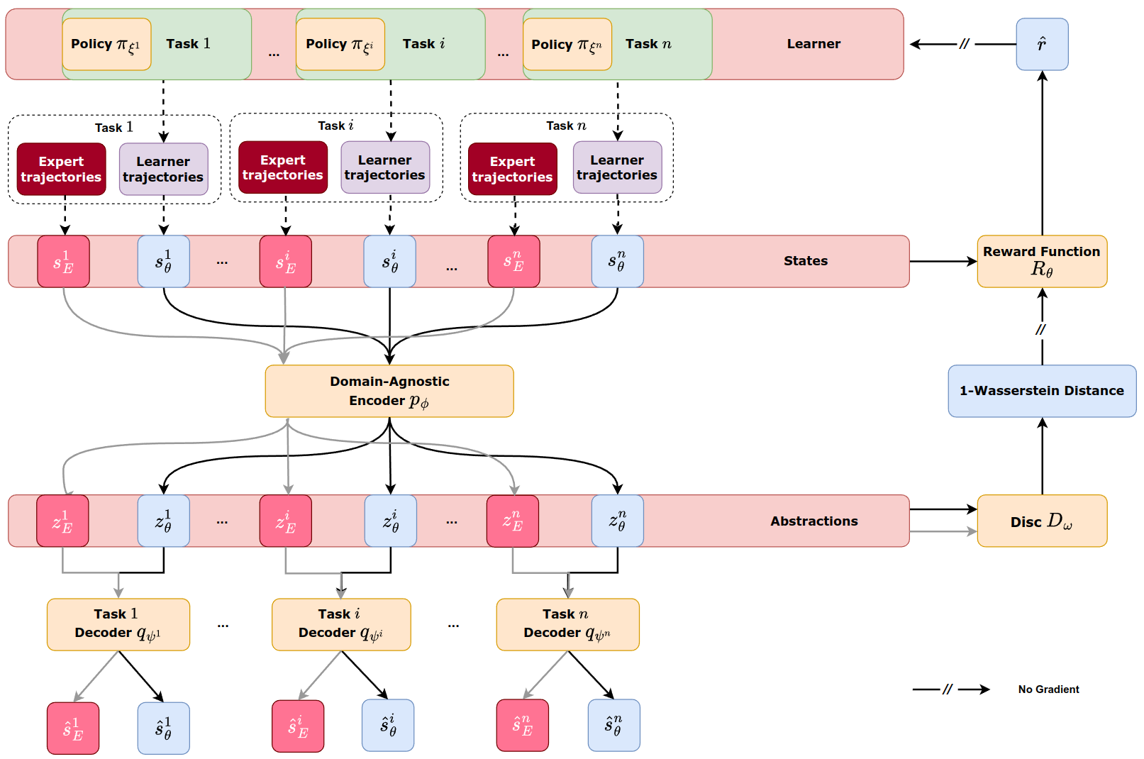
Figure 1: A visualization of the TraIRL method. A multi-head VAE is introduced within the discriminator of a generator-discriminator model. The green boxes represent the aligned task environments sharing intrinsic preferences. The purple boxes represent the sampled learner trajectories from the environments. The solid arrow represents the forward updates with backpropagation gradients. The dashed arrow and solid arrow with double slash represent no-gradient forward updates.

4 Learning Transferable Rewards via Abstraction

We introduce our method for transferable IRL, labeled TraIRL, in this section. The approach learns an abstract state-only reward function optimized for transfer from expert trajectories in source tasks. This reward function is then employed to learn a well-performing policy in the target environment.

Our approach encapsulates a novel variational autoencoder within the generator-discriminator schema to learn an abstract state representation (Section 4.1). In Section 4.2, we present an estimation of 1-Wasserstein distance, computed via the discriminator, which is utilized to learn an abstract reward function. Finally, Section 4.3 provides the analytic gradient formulation for the reward function since directly calculate the gradient w.r.t reward function is infeasible, enabling efficient and transferable reward learning across diverse environments.

4.1 Learning Abstraction via Multi-Head VAE

To enable reward transfer across different environments, it is important to identify and extract the intrinsic, abstract information that is invariant and generalizable from the source task demonstrations. In TraIRL, we use a variational autoencoder (VAE) (Kingma and Welling, 2014) to learn the abstraction from the experts’ and learner trajectory states. Recall that a VAE learns a joint distribution $p(x,z)$ over observed data $x$ and latent variables $z$ by maximizing the evidence lower bound (ELBO): $\mathcal{L}({\bm{\phi}},{\bm{\psi}};x)=\mathbb{E}_{p_{\bm{\phi}}(z|x)}\left[\log q_{\bm{\psi}}(x|z)\right]-\mathcal{D}_{\text{KL}}\left(p_{\bm{\phi}}(z|x)||p(z)\right)$ where $q_{\bm{\psi}}$ is the decoder’s variational approximation parameterized by ${\bm{\psi}}$, ${\bm{\phi}}$ parameterizes the encoder, and $\mathcal{D}_{\text{KL}}(\cdot||\cdot)$ is the forward KL divergence.

To learn the abstraction from the trajectories in the source environments, we use a single environment-agnostic encoder (denoted by $p_{\bm{\phi}}$ in Fig. 1) to obtain the latent variables, which serve as the abstraction, and $n$ environment-specific decoders ($q_{\psi^{i}}$ where $1\leq i\leq n$ denotes the $i$-th source task) to reconstruct the state trajectory of each environment. In the training phase, $p_{\bm{\phi}}$ learns the abstraction from generalizing the states of the source environments. The environment-specific decoders ($q_{\psi^{i}}$) learn to reconstruct the states of each environment from the abstraction.

The objective of our VAE is to minimize the novel loss function shown below, which incorporates the single encoder, $n$ environment-specific decoders, and aligns with the ELBO discussed previously.

$$\mathcal{L}_{\text{VAE}}({\bm{\phi}},\psi^{1},\ldots,\psi^{n};{\bm{\tau}})= \sum_{i=1}^{n}\left(\mathbb{E}_{z\sim p_{\bm{\phi}}(z^{i}|\tau^{i})}\left[\log q_{\psi^{i}}(\tau^{i}|z)\right]\right.$$

$$\left.-\lambda_{\mathcal{D}}~\mathcal{D}_{\text{KL}}\left(p_{\bm{\phi}}(z^{i}|\tau^{i})||p(z^{i})\right)\right),$$ (2)

where ${\bm{\tau}}\triangleq\langle\tau^{1},\tau^{2},\ldots,\tau^{i},\ldots,\tau^{n}\rangle$, and $\tau^{i}$ is a trajectory from the $i$-th source environment, $z\sim p_{\bm{\phi}}(z^{i}|\tau^{i})$ is the abstracted state sampled from the $i$-th source environment, $\lambda_{\mathcal{D}}$ is the hyperparameter controlling the magnitude of the loss of the forward KL divergence, and the prior $p(z^{i})=\mathcal{N}(0,1)$.

4.2 Learning Abstracted State Densities and Discriminator

Instead of having direct access to the experts’ policies or induced state probability densities, in practice, we are provided with expert demonstration trajectories. Recall that $f$-IRL’s loss function given by Eq. 1 uses the 1-Wasserstein distance to learn the reward function. We employ the Wasserstein-GAN (WGAN) (Arjovsky et al., 2017) to estimate the 1-Wasserstein distance between the expert and learner state distributions. Here, a discriminator network parameterized by ω, denoted by $D_{\bm{\omega}}$, is trained to approximate the 1-Wasserstein distance during each update iteration.

$$D_{\bm{\omega}}=\arg\max_{\bm{\omega}}\mathbb{E}_{s\sim\rho_{E}(s)}[D_{\bm{\omega}}(s)]-\mathbb{E}_{s\sim\rho_{\bm{\theta}(s)}}[D_{\bm{\omega}}(s)],$$ (3)

where $\rho_{\theta}$ is the state density of learner trajectories and $\rho_{E}$ is the state density of expert trajectories.

As our VAE extracts the abstraction $z$ by optimizing Eq. 2, we replace the state $s$ with the abstraction $z$ in the Eq. 3. The abstract state density $\rho(z)$ is defined as:

$$\rho(z) =\int_{s}\rho(z,s)ds=\int_{s}p_{\bm{\phi}}(z|s)\rho(s)ds$$ (4)

where $p_{\bm{\phi}}(z|s)$ represents encoder in the VAE. Substituting $z\sim\rho(z)$ into the Eq. 3, we obtain:

$$D_{\bm{\omega}}=\arg\max_{\bm{\omega}}\mathbb{E}_{z\sim\rho_{E}(z)}[D_{\bm{\omega}}(z)]-\mathbb{E}_{z\sim\rho_{\bm{\theta}}(z)}[D_{\bm{\omega}}(z)],$$ (5)

where $\rho_{\bm{\theta}}(z)$ and $\rho_{E}(z)$ denote the abstract state densities of the learner and expert trajectories, respectively.

To ensure the stability of training and enforce the 1-Lipschitz constraint required by WGAN, we further impose a gradient penalty on the discriminator (WGAN-GP) (Gulrajani et al., 2017). The gradient penalty is applied by adding a regularization term to the discriminator’s objective function:

$$\mathbb{E}_{z\sim\hat{\rho}(z)}\left[\left(\|\nabla_{z}D_{\bm{\omega}}(z)\|_{2}-1\right)^{2}\right],$$ (6)

where $\hat{\rho}(z)$ is the distribution of points $z$ sampled uniformly along a straight line between the abstract states of experts drawn from $\rho_{E}(z)$ and the abstract states of students drawn from $\rho_{\bm{\theta}}(z)$. This penalty encourages the norm of the discriminator gradient with respect to its inputs to be close to 1, satisfying the Lipschitz constraint.

By optimizing the discriminator with this additional gradient penalty, we ensure a more stable training process while preserving the estimation of the 1-Wasserstein distance between the expert and the learner in the abstract state space. Thus, the objective function for the discriminator becomes:

$$\begin{split}\mathcal{L}_{\mathcal{D}}({\bm{\omega}})=&\mathbb{E}_{z\sim\rho_{E}(z)}\left[D_{\bm{\omega}}(z)\right]-\mathbb{E}_{z\sim\rho_{\bm{\theta}}(z)}\left[D_{\bm{\omega}}(z)\right]\\ &+\lambda_{\text{GP}}~\mathbb{E}_{z\sim\hat{\rho}(z)}\left[\left(\|\nabla_{z}D_{\bm{\omega}}(z)\|_{2}-1\right)^{2}\right],\end{split}$$ (7)

where $\lambda_{\text{GP}}$ is a regularization coefficient that controls the magnitude of the gradient penalty.

4.3 Robust Transferable Reward Learning via Abstracted State Density

Once estimation of the 1-Wasserstein distance is learned, we can recover the reward function based on this estimation for the $i$-th source task analogously to Eq. 1 by substituting the states $s$ with the abstracted states $z^{i}$ for the $i$-th source environment.

$$\mathcal{L}^{i}_{\mathcal{F}}({\bm{\theta}},{\bm{\phi}}) =W_{1}(\rho_{E}(z^{i}),\rho_{\bm{\theta}}(z^{i}))$$

$$=\sup_{||f||_{L}\leq 1}\left|\mathbb{E}_{z\sim\rho_{E}(z^{i})}[f(z)]-\mathbb{E}_{z\sim\rho_{\bm{\theta}}(z^{i})}[f(z)]\right|$$

$$=\max_{D_{\bm{\omega}}}\mathbb{E}_{z\sim\rho_{E}(z^{i})}[D_{\bm{\omega}}(z)]-\mathbb{E}_{z\sim\rho_{\bm{\theta}}(z^{i})}[D_{\bm{\omega}}(z)],$$ (8)

where $W_{1}$ denotes the 1-Wasserstein distance, $p_{\bm{\phi}}$ is the encoder in VAE, and $\rho_{\bm{\theta}}(z)$ represents the abstract state density of the learner policy optimized by the reward function $r_{\bm{\theta}}$. Since the objective function $\mathcal{L}^{i}_{\mathcal{F}}({\bm{\theta}},{\bm{\phi}})$ involves both ${\bm{\theta}}$ and ${\bm{\phi}}$, optimizing the 1-Wasserstein distance in terms of encoder $p_{\bm{\phi}}$ helps shape a more generalized abstract state space. The gradient of this objective function w.r.t. ${\bm{\theta}}$ is provided in the Appendix A.

Theorem 1 (Gradient).

The analytic gradient of our objective function $\mathcal{L}_{f}^{i}({\bm{\theta},\bm{\phi}})$ presented in Eq.8 w.r.t ${\bm{\theta}}$ can be derived as: $\begin{aligned} &\nabla_{\bm{\theta}}\mathcal{L}^{i}_{\mathcal{F}}({\bm{\theta}},{\bm{\phi}})=\\ &\frac{1}{\alpha T}\text{cov}_{\tau\sim\hat{\rho}(\tau^{i})}\left(\sum^{T}_{t=1}\mathbb{E}_{z\sim p_{\bm{\phi}}(z_{t}|s_{t})}\left[D_{\bm{\omega}}(z)\right],\sum^{T}_{t=1}\nabla_{\bm{\theta}}r_{\bm{\theta}}(s_{t})\right),\end{aligned}$ where $\hat{\rho}(\tau^{i})=\frac{1}{2}(\rho_{\bm{\theta}}(\tau^{i})+\rho_{E}(\tau^{i}))$.

By deriving the gradient in the context of the 1-Wassersterin distance between state density and abstract density, the optimization to inversely learn the reward function is explicitly tied to the abstract states. As such, the learned reward function operates in the abstract state space, focusing on intrinsic features that are shared across the source domains. This focus on shared intrinsic preferences allows the reward function to generalize effectively across diverse domains, offering a robust foundation for transferring rewards from source to target environments.

The overall objective function for TraIRL involving $n$ source domains is a linear combination of the three loss functions defined previously:

$$\mathcal{L}({\bm{\theta}},{\bm{\omega}},{\bm{\phi}},{\bm{\psi}^{1}},\dots,{\bm{\psi}^{n}})$$

$$=\sum_{i=1}^{n}\mathcal{L}_{\mathcal{F}}^{i}({\bm{\theta}},{\bm{\phi}})-\mathcal{L}_{\text{VAE}}({\bm{\phi}},{\bm{\psi}^{1}},\dots,{\bm{\psi}^{n}})-\mathcal{L}_{D}({\bf\bm{\omega}}).$$ (9)

Fu et al. (2018) emphasize that reward functions disentangled from environment dynamics are desirable for transfer, as they generalize across different environments. They show that a reward function must be state-only to be dynamics-agnostic, but the converse does not hold—a state-only reward does not guarantee independence from dynamics. In our approach, the abstracted state representation is designed to remain invariant to the dynamics. By training the VAE and the discriminator across multiple source environments, we aim to learn an abstraction that generalizes well and is robust to changes in dynamics. This facilitates shaping the state-only reward function learned by TraIRL to yield dynamic-agnostic behavior, improving transferability across environments. Of course, extracting common (invariant) features across different tasks should further aid learning a transferable reward function. TraIRL fulfills this desiderata through its use of a multi-head VAE to learn abstracted representations from the states.

Definition 1 (Reward Transferability).

Define a reward function $r_{\bm{\theta}}$ learned for states $\mathcal{S}$ of the source environments as transferable to a target environment $\mathcal{T}$ iff for a small positive constant $\epsilon>0$,

$$W_{1}(\rho_{\mathcal{T}}^{*}(z),\rho_{\mathcal{T}}(z))\leq\epsilon,$$ (10)

where $\rho_{\mathcal{T}}^{*}$ is the abstract state density induced by the (soft-)optimal policy $\pi^{*}_{\mathcal{T}}$ in the target and $\rho_{\mathcal{T}}$ is the abstract state density induced by the policy $\pi_{\mathcal{T}}$ obtained by optimizing for $r_{\bm{\theta}}$ in the target.

While the learned state-only rewards are not a direct function of the abstraction, the learning of the rewards involves the discriminator utilizing the abstraction as its input. This discriminator is optimized to distinguish between the distributions over the abstract states induced by the expert demonstrations and the learner policy. The reward function is then shaped by the 1-Wasserstein distance over the abstracted state space provided by this discriminator.

Next, Theorem 2 delineates the conditions under which the reward function learned using TraIRL is transferable from source environments to a target environment. It leverages the abstract state densities, which capture the intrinsic features shared across the sources and with the target task.

Theorem 2 (Applicability of TraIRL).

Let $r_{\bm{\theta}}$ denote the reward function learned by optimizing Eq. 8, $\rho_{\mathcal{S}^{i}}^{*}(z)$ denote the abstract state density of the expert in the $i$-th source environment $\mathcal{S}^{i}$, $\epsilon$ be the positive threshold from Def. 1. If, for every $i$,

$$W_{1}(\rho_{\mathcal{T}}^{*}(z),\rho_{\mathcal{S}^{i}}^{*}(z)) \leq\epsilon/2$$ (11)

$$W_{1}(\rho_{\mathcal{T}}(z),\rho_{\mathcal{S}^{i}}^{*}(z)) \leq\epsilon/2$$ (12)

then the reward function $r_{\bm{\theta}}$ is transferable to the target environment, enabling effective policy learning.

Proof.

Wasserstein distance, $W_{1}$, satisfies the triangle inequality. Applying it to Eqs. 11 and 12, we derive Eq. 10. This satisfies the transferable reward condition in Def 1. ∎

Algorithm 1 demonstrates the training procedure for TraIRL. During each iteration, trajectories are uniformly sampled from each source environment and added to the buffer (line 9). The encoder $p_{\bm{\phi}}$, decoders $q_{\bm{\psi}^{1}},...,q_{\bm{\psi}^{n}}$, and discriminator $D_{\bm{\omega}}$ are updated first (lines 10-12). Then the reward function $R_{\bm{\theta}}$ is updated using the updated encoder $p_{\bm{\phi}}$ and discriminator $D_{\bm{\omega}}$ (line 13). Lastly, the learner policies $\pi_{\bm{\xi}^{1}},...,\pi_{\bm{\xi}^{n}}$ are updated in the source environments $\mathcal{S}^{1},...,\mathcal{S}^{n}$ using the updated reward function $D_{\bm{\omega}}$, respectively (line 14).

Algorithm 1 TraIRL: Training Phase

1:Expert trajectories $\tau^{1}_{E},...,\tau^{n}_{E}$, Source environments: $\mathcal{S}^{1},...,\mathcal{S}^{n}$

2:Initialize learner policies $\pi_{\bm{\xi}^{1}},...,\pi_{\bm{\xi}^{n}}$, Trajectory buffer $B$, Discriminator $D_{\bm{\omega}}$, Reward function $R_{\bm{\theta}}$, encoder $p_{\bm{\phi}}$, and decoders $q_{\bm{\psi}^{1}},...,q_{\bm{\psi}^{n}}$

3:Add expert trajectories $\tau^{1}_{E},...,\tau^{n}_{E}$ into trajectory buffer $B$

4:while $\pi_{\xi^{1}},...,\pi_{\xi^{n}}$ continue improving within $k$ steps do

5:  for env $i$ in ${1,...,n}$ do

6:    Collect state-only trajectories $\tau^{i}=(s_{0},...,s_{T})$

7:    Add trajectories $\tau^{i}$ into trajectory buffer $B$

8:  end for

9:  Uniformly sample trajectories $\bar{\tau}$ from Buffer $B$

10:  Update $q_{\bm{\psi}^{1}},...,q_{\bm{\psi}^{n}}$ using $\bar{\tau}$ by Eq. 2

11:  Update $p_{\bm{\phi}}$ using $\bar{\tau}$ by Eq. 2 and Eq. 8

12:  Update $D_{\bm{\omega}}$ using $\bar{\tau}$ by Eq. 7

13:  Update $R_{\bm{\theta}}$ using $\bar{\tau}$ by Eq. 8

14:  Update $\pi_{\bm{\xi}^{1}},...,\pi_{\bm{\xi}^{n}}$ using $R_{\bm{\theta}}$

15:end while

Algorithm 2 TraIRL: Transfer Testing Phase

1:Reward function $R_{\theta}$ learned by Algorithm 1, Target Environment $\mathcal{T}$

2:Initialize policy $\pi_{\xi}$

3:while $\pi_{\xi}$ continues improving within $k$ steps do

4:  Update $\pi_{\xi}$ only using the learned reward function $R_{\theta}$ in target environment $\mathcal{T}$

5:end while

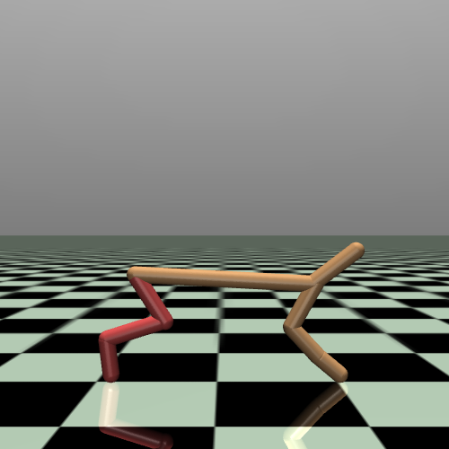
(a)

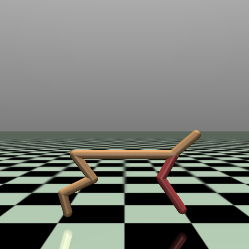
(b)

(c)

(d)

(e)

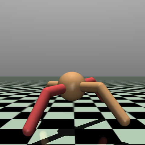
(f)

Figure 2: Formative source and target environments from MuJoCo-Gym domains. The red legs are the disabled legs of the robots. Frames $(a,b)$ depict the source tasks of running with a disabled leg in Half Cheetah, while $(c)$ represents the target environment with no disability. Similarly, frames (d,e) show the source tasks of running with different pairs of disabled legs in Ant, whereas (f) shows the target task of running with another pair of disabled legs.

5 Experiments

We implement Algorithms 1 and 2 in PyTorch, and empirically evaluate the performance of TraIRL across MuJoCo benchmark domains (Todorov et al., 2012) and across the human-robot Assistive Gym domains (Erickson et al., 2019). TraIRL is run on 50 trajectories of two distinct source tasks with different dynamics, from these domains. It is run until convergence on each trajectory, defined as the stabilization of cumulative rewards obtained from forward RL using both the learned and ground-truth reward functions. To evaluate TraIRL’s reward transferability, we use forward RL with the inversely learned rewards in the target environment to obtain the policy (from scratch). Note that we do not use the target’s true rewards and utilize the learned reward function only. We measure how well this policy performs by simulating it for 25 episodes and reporting the mean of the accumulated rewards.

We adopt a similar procedure for three state-of-the-art baseline techniques, which were previously discussed in the paper: AIRL, $f$-IRL, and I2L. Although AIRL and $f$-IRL were not explicitly designed for reward transferability, their respective expositions suggest that these methods can generalize rewards across environments with shifting dynamics. However, their reliance on single-environment training may limit adaptability to varying dynamics, which we evaluate in the experiments. In contrast, I2L is designed to handle such shifts and potentially offers better cross-environment generalization, though without any abstraction mechanisms, as used by TraIRL.

Model architecture and implementation   We employ a multilayer perceptron with Tanh as the activation function for both the encoder and the decoder in the VAE and to represent the reward function. TraIRL and all baselines have been implemented in PyTorch. We choose reverse KL divergence as the objective function in $f$-IRL because it has been shown to be robust and faster to converge for IRL compared to regular KL divergence (Ni et al., 2021; Ghasemipour et al., 2020). Forward RL in the environments is performed using the Soft Actor-Critic (SAC) (Haarnoja et al., 2018). Further details regarding the model architecture and hyperparameters to aid reproducibility are available in the Appendix C.

5.1 Formative Evaluations in MuJoCo-Gym

Two source environments and one target environment from each of the Half Cheetah and Ant domains in MuJoCo-Gym are used. Figure 2 illustrates the source and target environments, which differ in dynamics between the sources and between the sources and the target. Specifically, these differences in dynamics arise from disabling different pairs of legs. Disabled legs are indicated in red in the frames of Fig. 2. While the action space remains unchanged across the environments, as the applied forces are directed to all joints regardless of whether a leg is disabled, the dynamics differ because the disabled legs cannot respond to the input actions.

5.1.1 Reward Transferability

Tables 1 and 2 report our results using TraIRL and the baselines on Half Cheetah and Ant domains, respectively. These show the mean cumulative rewards obtained in the target environment as well as in the two source environments. The optimal policy’s (expert) rewards for each are reported as well, to provide an upper bound.

Observe that the rewards learned by TraIRL achieve the highest average return compared to all baselines in the target environment for both domains. As such, the abstracted rewards learned by TraIRL from the two sources are most transferable. I2L’s learned rewards yield the next best performance on the target task but remain significantly lower than TraIRL’s (Student’s paired t-test, $p<0.01$). Other baselines learned reward functions that do not transfer to the target. However, the reward transferred to the target half cheetah that has no disability focuses on its torso and does not encourage coordinated leg movement, resulting in a performance drop compared to the optimal.

	Sources		Target
	Run (rear disabled)	Run (front disabled)	Run (no disability)
AIRL	2,573.91 $\pm$ 82.5	1,576.82 $\pm$ 529.9	2,683.81 $\pm$ 163.8
$f$-IRL	3,252.72 $\pm$ 67.9	3,523.01 $\pm$ 91.1	3,582.10 $\pm$ 94.3
I2L	4,396.43 $\pm$ 45.4	4,518.66 $\pm$ 52.2	4,512.71 $\pm$ 66.4
TraIRL	4,404.07 $\pm$ 57.6	4,359.35 $\pm$ 99.2	4,745.59 $\pm$ 48.6
Expert	5,052.25 $\pm$ 25.4	5,499.07 $\pm$ 156.1	7,589.52 $\pm$ 123.6

Table 1: Mean cumulative rewards with standard deviation for the methods in the Half Cheetah domain. TraIRL has the highest cumulative reward in the target task and the improvement over I2L is significant.

	Sources		Target
	Run (1,2 disabled)	Run (2,3 disabled)	Run (1,3 disabled)
AIRL	1,918.28 $\pm$ 76.3	1,415.76 $\pm$ 83.8	947.00 $\pm$ 37.8
$f$-IRL	2,456.17 $\pm$ 85.0	1,146.39 $\pm$ 95.8	1,598.24 $\pm$ 44.9
I2L	2,831.28 $\pm$ 36.4	2,786.90 $\pm$ 79.4	2,585.32 $\pm$ 84.5
TraIRL	2,714.18 $\pm$ 35.9	2,936.52 $\pm$ 95.5	2,917.92 $\pm$ 79.3
Expert	3,312.12 $\pm$ 304.3	3,303.99 $\pm$ 341.0	3,369.05 $\pm$ 216.8

Table 2: Mean cumulative rewards with standard deviation for the Ant domain. TraIRL has the highest cumulative reward in the target task followed by I2L again.

It is worth analyzing the IRL’s performance on the source environments as well. TraIRL remains competitive – learning rewards that yield comparatively the best policy for the first source task of Half Cheetah and the second source task of Ant. In the other source tasks, it closely trails I2L’s performance. Overall, these learned rewards yield policies that are close to the optimal for the source tasks.

5.1.2 Benefit of Using Abstractions and its Visualization

To understand why TraIRL performs better, we aim to gain some insight into our novel abstraction concept. Recall that the abstract state densities are learned via the VAE and the 1-Wasserstein distance $W_{1}$ between the densities is obtained from the discriminator $D_{\bm{\omega}}$. In Table 3, we report this distance between the converged densities of the two source tasks and between the densities of the target and each source, for the Half Cheetah domain. We compare these to the corresponding $W_{1}$ distances between the (ground) state densities. To obtain the Wasserstein distance between state densities, we train a variant of $f$-IRL that replaces the $f$-divergence with the 1-Wasserstein distance (see Appendix A.2 of (Ni et al., 2021)). To obtain the distances between the abstract state densities, we sample states from the source and target environments and input them into TraIRL.

	State	Abstraction
Run (rear disabled) and Run (front disabled)	1.37	1.24
Run (rear disabled) and Run (no disability)	2.83	1.46
Run (front disabled) and Run (no disability)	2.10	1.59

Table 3: Abstraction yields a smaller 1-Wasserstein distance in the Half Cheetah environment, which is desirable.

For each comparison (row) in Table 3, the abstracted state densities yield a lower $W_{1}$ distance compared to the (ground) state densities. This implies that the shaped latent embeddings ($Z$) serve to bring the compact state representations of the two environments closer, contributing to better generalizability.

Next, Figure 3 visualizes the t-SNE (Van der Maaten and Hinton, 2008) of the VAE-induced abstractions and (ground) states for our two source tasks in the Half Cheetah domain. There is a clear separation between the abstraction embeddings of the expert and the learner in Fig. 3(a). More importantly, the t-SNEs of the two source tasks are intermingled due to the abstraction, which is another indication of the spaces of the two tasks coming together. In contrast, Fig. 3(b) shows that the t-SNEs of the trajectory states of the two source tasks appear in separated clusters. Furthermore, there is no single plane separating the embeddings of the expert and learner-induced states from their trajectories.

We also explored the sensitivity of TraIRL’s performance to values of hyperparameters $\lambda_{\mathcal{D}}$ in Eq. 2 and $\lambda_{\text{GP}}$ in Eq. 7, and present the results in Appendix B.

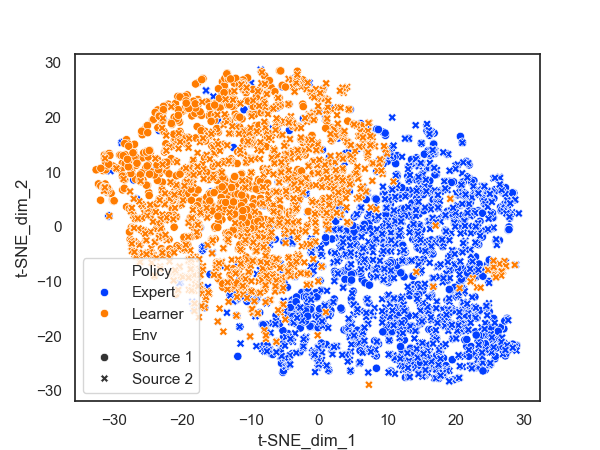
(a) Abstractions

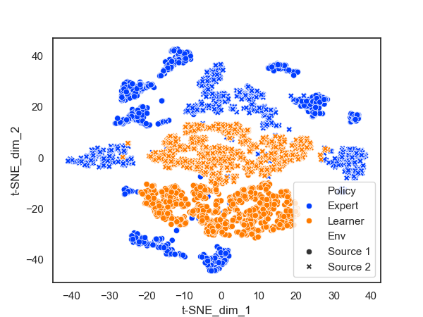
(b) States

Figure 3: Visualization of distributions of t-SNE of sampled abstractions and states for the Half Cheetah source environments.

(a) FeedingSawyer

(b) ScratchItchSawyer

Figure 4: $(a)$ Two tasks in this environment are used as sources to learn a reward function that can be transferred to perform the task of $(b)$ scratching an itch.

5.2 Summative Evaluation in Human-Robot Assistive Gym

To give an indication of the utility of TraIRL in the real-world, we illustrate its use in human-robot collaboration using the highly realistic Assistive Gym testbed (Erickson et al., 2019). Similar to MuJoCo, Assistive Gym is a physics-based simulation framework but for human-robot interaction and robotic assistance by the collaborative robot Sawyer. It consists of a suite of simulation environments for six tasks associated with activities of daily living such as itch scratching, bed bathing, drinking water, feeding, dressing, and arm manipulation. A key difference between the MuJoCo environments and Assistive Gym is the form of the reward functions. Environments in Assistive Gym have rewards that are much more sparse than those in MuJoCo. For instance, in the FeedingSawyer environment, if the robot spills food from the spoon, it enters a terminal state with a penalty of 1. Conversely, if the robot successfully feeds the human, it receives a +10 reward upon reaching the terminal state. No other rewards are given to the robot. Another difference is that the MuJoCo environments we use do not have terminal states with high rewards or penalties.

For the source environments, we select FeedingSawyer, a simulation environment in which the collaborative robot is tasked with feeding a disabled human. The two source environments differ in the condition of the disabled human. The human is static in one while the human has tremors in the other, which cause the target area to move resulting in a shifting goal. The robot’s challenge is to adapt to these differing human conditions while executing the feeding task. Our target environment is a different task, ScratchItchSawyer, in which Sawyer is tasked with scratching a disabled human’s itch. Although this task differs from feeding in terms of its specific goal, they are also similar in that the robot must move its end effector precisely to a designated target area.

	Sources		Target
	Feeding task 1	Feeding task 2	Scratch itch
AIRL	-13.22 $\pm$ 13.56	-18.3 $\pm$ 19.26	-22.36 $\pm$ 15.31
$f$-IRL	-10.63 $\pm$ 16.79	-15.3 $\pm$ 22.78	-21.35 $\pm$ 14.89
I2L	9.32 $\pm$ 11.8	9.11 $\pm$ 11.36	-10.07 $\pm$ 8.02
TraIRL	8.32 $\pm$ 7.9	9.56 $\pm$ 10.52	-3.82 $\pm$ 3.33
Expert	11.29 $\pm$ 5.39	12.77 $\pm$ 4.28	-1.18 $\pm$ 5.71

Table 4: Actual cumulative reward with standard deviation in the Assistive Gym environments. TraIRL has the highest cumulative reward in the target domain.

We report the performance of TraIRL and the baselines in transferring the reward function inversely learned from the two feeding tasks, to learn how to scratch the person’s itch. Table 4 gives the mean cumulative reward from forward RL in the target using the learned rewards. Notice that TraIRL yields the policy with the highest reward and close to the optimal, indicating transferable rewards. The transferred reward function exhibits a strong positive linear relationship with the true rewards, as indicated by a Pearson correlation coefficient of 0.8553 ($p<.001$). This high correlation suggests that TraIRL’s learning process effectively approximates the true reward function of ScratchItchSawyer, demonstrating the reliability of the learned rewards in the target environment.

The AIRL and $f$-IRL baselines show poor transferability whereas I2L performs significantly better than them, but still worse than TraIRL. Analogously to the results in MuJoCo, I2L or TraIRL learn comparative reward functions from the source tasks’ trajectories. The poor transferability of AIRL and $f$-IRL is partly because both methods fail to inversely learn the expert’s reward function in the source tasks correctly.

6 Conclusion

TraIRL represents a significant advancement of IRL by introducing a principled approach to inversely learn transferable reward functions from demonstrations in multiple environments. The key innovation lies in the ability to extract invariant abstractions that encode the structure intrinsic to multiple trajectories, which makes them transferable to aligned target tasks. TraIRL’s analytical properties delineate the transfer applicability of the abstracted rewards and the experiments validate the transferability in both formative and use-inspired contexts. Future work could investigate general ways of quickly fine-tuning the transferred reward function to improve its fit for a broader family of target tasks.

Appendix A Analytical Gradient of TraIRL (Theorem 1)

In this section, we derive the analytic gradient of the proposed TraIRL (Theorem 1). From [Ni et al., 2021], we have the following equations:

$$\begin{split}\frac{d\rho_{\theta}(s)}{d\theta}&=\int\frac{d\rho_{\theta}(s)}{dr_{\theta}(s^{*})}\frac{dr_{\theta}(s^{*})}{d\theta}ds^{*}\\ &=\frac{1}{\alpha Z}\int p(\tau)e^{\sum^{T}_{t=1}r_{\theta}(s_{t})/\alpha}\eta_{\tau}(s)\sum^{T}_{t=1}\frac{dr_{\theta}(s_{t})}{d\theta}d\tau-\frac{T}{\alpha}\rho_{\theta}(s)\int\rho_{\theta}(s^{*})\frac{dr_{\theta}(s^{*})}{d\theta}ds^{*},\end{split}$$ (13)

where $\alpha$ is the entropy temperature.

The joint distribution over state and abstractions is defined as:

$$\begin{split}\rho(z,s)&=p_{\bm{\phi}}(z|s)\rho(s),\\ \end{split}$$ (14)

where $p_{\bm{\phi}}(z|s)$ is the encoder parameterized by ${\bm{\phi}}$.

The marginal distribution of the abstraction $z$, denoted as the abstract state density $\rho(z)$, is obtained by integrating out the state $s$ from Eq. 14:

$$\rho(z) =\int_{s}\rho(z,s)ds$$

$$=\int_{s}p_{\bm{\phi}}(z|s)\rho(s)ds.$$

When optimizing the abstract state density matching objective between the expert density $\rho_{E}(z)$ and the learner density $\rho_{\bm{\theta}}(z)$ in the $i$-th source environment, we measure their discrepancy using 1-Wasserstein distance. The objective is formulated as:

$$\mathcal{L}^{i}_{\mathcal{F}}({\bm{\theta},\bm{\phi}}) =W_{1}(\rho_{E},\rho_{\bm{\theta}})$$

$$=\sup_{||f||_{L}\leq 1}\left|\mathbb{E}_{z\sim\rho_{E}(z^{i})}[f(z)]-\mathbb{E}_{z\sim\rho_{\bm{\theta}}(z^{i})}[f(z)]\right|$$

$$=\max_{D_{\bm{\omega}}}\mathbb{E}_{z\sim\rho_{E}(z^{i})}[D_{\bm{\omega}}(z)]-\mathbb{E}_{z\sim\rho_{\bm{\theta}}(z^{i})}[D_{\bm{\omega}}(z)]$$

$$=\max_{D_{\bm{\omega}}}\int_{z^{i}}D_{\bm{\omega}}(z)\rho_{E}(z)dz-\int_{z^{i}}D_{\bm{\omega}}(z)\rho_{\bm{\theta}}(z)dz.$$

The objective is derived using the Kantorovich–Rubinstein duality, which reformulates the 1-Wasserstein distance as a supremum over all 1-Lipschitz functions. To approximate this function, we introduce a discriminator $D_{\bm{\omega}}(z)$ and express the optimization as a maximization of the expected difference between expert and learner distributions. To ensure that $D_{\bm{\omega}}(z)$ satisfies the 1-Lipschitz constraint required by the duality, we apply a gradient penalty, which also stabilizes optimization while preserving theoretical correctness.

The gradient of the objective w.r.t $\bm{\theta}$ is derived as:

$$\begin{split}\nabla_{\bm{\theta}}\mathcal{L}^{i}_{\mathcal{F}}({\bm{\theta},\bm{\phi}})&=-\int_{z^{i}}D_{\bm{\omega}}(z)\nabla_{\bm{\theta}}\rho_{\bm{\theta}}(z)dz\\ &=-\int_{z^{i}}\int_{s^{i}}D_{\bm{\omega}}(z)p_{\bm{\phi}}(z|s)\nabla_{\bm{\theta}}\rho_{\bm{\theta}}(s)dsdz.\\ \end{split}$$ (15)

Substituting the gradient of abstract state density $\rho_{\bm{\theta}}(z)$ w.r.t $\theta$ with Eq.13, we have:

$$\begin{split}\nabla_{\bm{\theta}}\mathcal{L}^{i}_{\mathcal{F}}({\bm{\theta},\bm{\phi}})&=\frac{1}{\alpha T}\mathbb{E}_{\tau\sim\rho_{\bm{\theta}}(\tau^{i})}\left[\sum^{T}_{t=1}\int_{z^{i}}D_{\bm{\omega}}(z)p_{\bm{\phi}}(z|s_{t})dz\right]\sum^{T}_{t=1}\frac{dr_{\bm{\theta}}(s_{t})}{d{\bm{\theta}}}-\frac{T}{\alpha}\mathbb{E}_{s\sim\rho_{\bm{\theta}}(s^{i})}\left[\int_{z^{i}}D_{\bm{\omega}}(z)p_{\bm{\phi}}(z|s)dz\right]\mathbb{E}_{s\sim\rho_{\bm{\theta}}(s^{i})}\left[\frac{dr_{\bm{\theta}}(s)}{d{\bm{\theta}}}\right]\\ &=\frac{1}{\alpha T}\mathbb{E}_{\tau\sim\rho_{\bm{\theta}}(\tau^{i})}\left[\sum^{T}_{t=1}\mathbb{E}_{z\sim p_{\bm{\phi}}(z_{t}|s_{t})}\left[D_{\bm{\omega}}(z)\right]\right]\sum^{T}_{t=1}\frac{dr_{\bm{\theta}}(s_{t})}{d{\bm{\theta}}}-\frac{T}{\alpha}\mathbb{E}_{s\sim\rho_{\bm{\theta}}(s^{i})}\left[\mathbb{E}_{z\sim p_{\bm{\phi}}(z|s)}\left[D_{\bm{\omega}}(z)\right]\right]\mathbb{E}_{s\sim\rho_{\bm{\theta}}(s^{i})}\left[\frac{dr_{\bm{\theta}}(s)}{d{\bm{\theta}}}\right].\end{split}$$ (16)

To gain further intuition about this equation, we can express all the expectations in terms of trajectories:

$$\nabla_{\bm{\theta}}\mathcal{L}^{i}_{\mathcal{F}}({\bm{\theta},\bm{\phi}}) =\frac{1}{\alpha T}\left(\mathbb{E}_{\rho_{\bm{\theta}}(\tau^{i})}\left[\sum^{T}_{t=1}\mathbb{E}_{p_{\bm{\phi}}(z_{t}|s_{t})}\left[D_{\bm{\omega}}(z)\right]\sum^{T}_{t=1}\frac{dr_{\bm{\theta}}(s_{t})}{d{\bm{\theta}}}\right]-\mathbb{E}_{\rho_{\bm{\theta}}(\tau^{i})}\left[\sum^{T}_{t=1}\mathbb{E}_{p_{\bm{\phi}}(z|s)}\left[D_{\bm{\omega}}(z)\right]\right]\mathbb{E}_{\rho_{\bm{\theta}}(\tau^{i})}\left[\sum^{T}_{t=1}\nabla_{\bm{\theta}}r_{\bm{\theta}}(s_{t})\right]\right)$$

$$=\frac{1}{\alpha T}\text{cov}_{\tau\sim\rho_{\bm{\theta}}(\tau^{i})}\left(\sum^{T}_{t=1}\mathbb{E}_{z\sim p_{\bm{\phi}}(z_{t}|s_{t})}\left[D_{\bm{\omega}}(z)\right],\sum^{T}_{t=1}\nabla_{\bm{\theta}}r_{\bm{\theta}}(s_{t})\right).$$ (17)

When operating in high-dimensional observation domains, a significant impediment arises if the state visitation distributions induced by the learner’s current policy substantially diverge from the expert demonstration trajectories. Under such conditions of distributional mismatch, we empirically find that the gradient signal derived from our proposed objective function, Eq. 17, provides limited supervisory information to guide the policy optimization process. We follow the technique introduced by [Finn et al., 2016], mixing the data samples from expert trajectories with the learner trajectories. The revised objective function is given in the following.

$$\nabla_{\bm{\theta}}\mathcal{L}^{i}_{\mathcal{F}}({\bm{\theta},\bm{\phi}})=\frac{1}{\alpha T}\text{cov}_{\tau\sim\hat{\rho}(\tau^{i})}\left(\sum^{T}_{t=1}\mathbb{E}_{z\sim p_{\bm{\phi}}(z_{t}|s_{t})}\left[D_{\bm{\omega}}(z)\right],\sum^{T}_{t=1}\nabla_{\bm{\theta}}r_{\theta}(s_{t})\right),$$ (18)

where $\hat{\rho}(\tau^{i})=\frac{1}{2}(\rho_{\bm{\theta}}(\tau^{i})+\rho_{E}(\tau_{E}^{i}))$.

Appendix B Hyperparameter Sensitivity

In this section, we evaluate the sensitivity of TraIRL’s performance on the coefficients $\lambda_{\text{GP}}$ and $\lambda_{\mathcal{D}}$. The coefficient $\lambda_{\text{GP}}$ controls the magnitude of the gradient penalty when updating the discriminator (Eq. 7), while $\lambda_{\mathcal{D}}$ regulates the strength of the regularization term when updating the encoder (Eq. 2).

B.1 Sensitivity to Hyperparameter $\lambda_{GP}$

	Sources		Target
	Run (rear disabled)	Run (front disabled)	Run (no disability)
$\lambda_{\text{GP}}=1$	4,646.12 $\pm$ 40.6	4,602.13 $\pm$ 24.1	3,228.27 $\pm$ 185.5
$\lambda_{\text{GP}}=5$	4,498.74 $\pm$ 59.5	4,313.89 $\pm$ 54.4	3,989.06 $\pm$ 61.6
$\lambda_{\text{GP}}=10$	4,404.07 $\pm$ 57.63	4,359.35 $\pm$ 99.24	4,745.59 $\pm$ 48.56
$\lambda_{\text{GP}}=100$	172.69 $\pm$ 191.9	155.66 $\pm$ 159.59	150.41 $\pm$ 102.6
Expert	5,052.3 $\pm$ 25.4	5,499.07 $\pm$ 156.1	7,589.52 $\pm$ 123.6

Table 5: Mean cumulative reward with standard deviation in the Half Cheetah domain. $\lambda_{\text{GP}}=10$ yields the highest cumulative reward in the target domain.

The coefficient $\lambda_{\text{GP}}$ controls the magnitude of the gradient penalty when updating the discriminator (Eq. 7). Table 5 presents the mean cumulative reward with standard deviation for different values of $\lambda_{\text{GP}}$ in the Half Cheetah domain. The results demonstrate that $\lambda_{\text{GP}}$ significantly influences performance across both the source and target environments. Notably, when $\lambda_{\text{GP}}=10$, the model achieves the highest cumulative reward in the target domain (4745.59 $\pm$ 48.56), indicating that this setting balances the regularization effect of the gradient penalty. In contrast, setting $\lambda_{\text{GP}}$ too low ($\lambda_{\text{GP}}=1$) results in suboptimal performance, likely due to insufficient constraint on the discriminator. Recall that the 1-Lipschitz constraint is a crucial condition for the discriminator to approximate the 1-Wasserstein distance. If $\lambda_{\text{GP}}$ is too small, it may lead to a violation of this constraint, preventing an accurate approximation of the 1-Wasserstein distance. Consequently, Theorem 2 is not satisfied, undermining the theoretical guarantees of TraIRL. Conversely, an excessively large $\lambda_{\text{GP}}$ ($\lambda_{\text{GP}}=100$) drastically degrades performance across all environments, suggesting that an overly strong gradient penalty hinders learning by excessively constraining the discriminator. These findings emphasize the importance of tuning $\lambda_{\text{GP}}$ to maintain theoretical validity while achieving optimal generalization in the target domain.

B.2 Sensitivity to Hyperparameter $\lambda_{\mathcal{D}}$

	Sources		Target
	Run (rear disabled)	Run (front disabled)	Run (no disability)
$\lambda_{\mathcal{D}}=0.05$	4,323.23 $\pm$ 29.58	4,471.05 $\pm$ 56.21	4,541.09 $\pm$ 96.30
$\lambda_{\mathcal{D}}=0.1$	4404.07 $\pm$ 57.6	4,359.35 $\pm$ 99.2	4,745.59 $\pm$ 48.6
$\lambda_{\mathcal{D}}=0.25$	4,430.26 $\pm$ 62.7	4234.33 $\pm$ 84.0	4,548.23 $\pm$ 44.5
$\lambda_{\mathcal{D}}=0.5$	3,806.92 $\pm$ 85.3	3,888.79 $\pm$ 52.5	4,088.95 $\pm$ 83.8
Expert	5,052.25 $\pm$ 25.4	5,499.07 $\pm$ 156.1	7,589.52 $\pm$ 123.6

Table 6: Mean cumulative reward with standard deviation in the Half Cheetah domain. $\lambda_{\mathcal{D}}=0.1$ yields the highest cumulative reward in the target domain.

$\lambda_{\mathcal{D}}$ regulates the strength of the regularization term when updating the encoder (Eq. 2). Table 6 reports the mean cumulative reward across different values of $\lambda_{\mathcal{D}}$ in the Half Cheetah domain. At $\lambda_{\mathcal{D}}=0.1$, the model achieves the highest cumulative reward in the target environment (4745.59 $\pm$ 48.56), indicating that this value provides a balance for learning effective latent representations. Lowering $\lambda_{\mathcal{D}}$ to 0.05 slightly reduces performance in the target domain (4541.09 $\pm$ 96.30), suggesting that insufficient regularization may lead to suboptimal feature extraction. Increasing $\lambda_{\mathcal{D}}$ beyond 0.1 results in a noticeable performance degradation. At $\lambda_{\mathcal{D}}=0.25$, the reward declines to 4548.23 $\pm$ 44.49, and at $\lambda_{\mathcal{D}}=0.5$, it further drops to 4088.95 $\pm$ 83.82. This decline suggests that excessive regularization constrains the encoder, limiting its ability to adapt to the target task. The performance reduction is also observed in source environments, indicating that overly strong regularization affects overall learning stability.

Appendix C Training Details and Hyperparameters

In this section, we show the comprehensive training details and hyperparameters. We use Soft Actor-Critic (SAC) as our Maximum Entropy Reinforcement Learning (MaxEnt RL) algorithm due to its efficient exploration, stability in continuous control tasks, and improved sample efficiency. By maximizing both cumulative reward and entropy, SAC promotes diverse and robust policies. For implementation, we use the SAC provided by the widely adopted Python library Stable-Baselines 3.

To generate expert demonstrations, we first train SAC agents with 5 different random seeds in each source domain until convergence. The hyperparameters used for SAC training are listed in Table 7. The unlisted hyperparameter remains the default setting in Stable-Baselines 3. After convergence, we collect 50 expert trajectories from each source domain. These expert trajectories are then used for training the transferable reward function via TraIRL as well as other baseline methods.

	Ant	HalfCheetah	FeedingSawyer	ScratchItchSawyer
Learning rate	$3e^{-4}$	$3e^{-4}$	$3e^{-4}$	$3e^{-4}$
Gamma	$0.95$	$0.95$	$0.95$	$0.95$
Batch size	$256$	$256$	$256$	$256$
Net arch	$[400,300]$	$[400,300]$	$[400,400]$	$[400,400]$
Buffer size	$1,000,000$	$1,000,000$	$1,000,000$	$100,000$
Action noise	$\mathcal{N}(0,0.2)$	$\mathcal{N}(0,0.2)$	$\mathcal{N}(0,0.2)$	$\mathcal{N}(0,0.25)$

Table 7: Hyperparameter setting of SAC.

Next, we begin training TraIRL. The hyperparameters used in each source domain are listed in Table 8. Notably, the SAC in TraIRL adopts the same hyperparameters specified in Table 7. The net arch represents the dimensions of the model for each layer, excluding the output layer. The reward function produces a single scalar value, which is activated by a Sigmoid function. The update step refers to the number of gradient updates performed during each iteration of the training process, where one iteration corresponds to the steps outlined in Line 10–14 of Algorithm 1.

	Ant	HalfCheetah	FeedingSawyer
$\lambda_{\text{GP}}$	$10$	$10$	0.01
$\lambda_{\mathcal{D}}$	$0.1$	$0.1$	0.1
Reward Function Hyperparameter
Learning Rate	3e-4	3e-4	5e-4
Batch Size	128	128	128
Weight Decay	1e-3	1e-3	1e-3
Net arch	[16, 16]	[16, 16]	[16, 16]
Activation	Tanh	Tanh	Tanh
Reward Update Steps	200	200	200
VAE and Discriminator Hyperparameter
Learning Rate	3e-4	3e-4	5e-4
Batch Size	128	128	128
Weight Decay	1e-3	1e-3	1e-3
Encoder Net Arch	[32, 32]	[32, 32]	[16, 16]
Encoder Activation	Tanh	Tanh	Tanh
Abstraction Dimension	27	17	4
Decoder Net Arch	[32, 32, 32]	[32, 32, 32]	[16, 16, 16]
Decoder Activation	Tanh	Tanh	Tanh
VAE Update Steps	200	200	200
Discriminator Net Arch	[32, 32]	[32, 32]	[16, 16]
Discriminator Activation	Tanh	Tanh	Tanh
Disc Update Steps	200	200	200

Table 8: Hyperparameter setting of TraIRL (Algorithm 1).

After training TraIRL, we obtain a trained transferable reward function, which is then applied to the target domain by replacing the original reward function. Consequently, when the agent interacts with the target domain, it only has access to the trained reward function. We continue to use SAC with the hyperparameters specified in Table 7 for policy optimization in the target domain.

(a) Training curve in Half Cheetah (rear disabled).

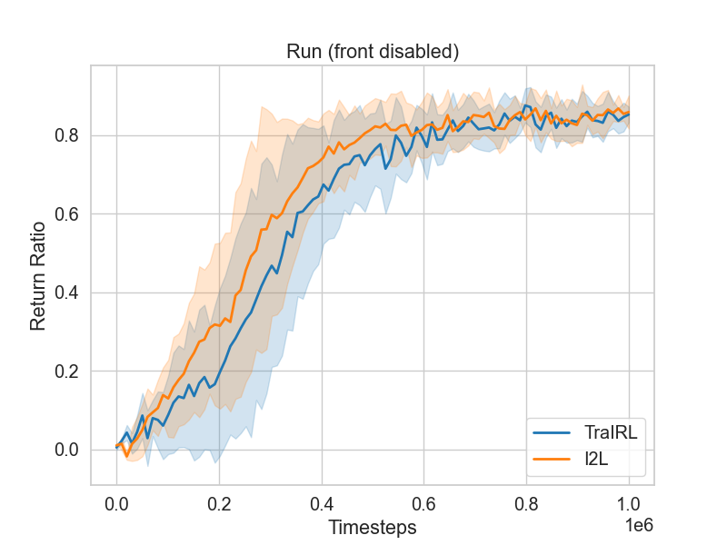
(b) Training curve in Half Cheetah (front disabled)

Figure 5: Training curve for Half Cheetah Environment including both source domains. The true cumulative reward is used here for evaluation. AIRL and $f$-IRL perform poorly in the experiments and are therefore excluded from the comparison.

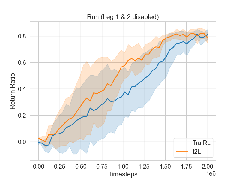
(a) Training curve in Ant (Leg 1 & 2).

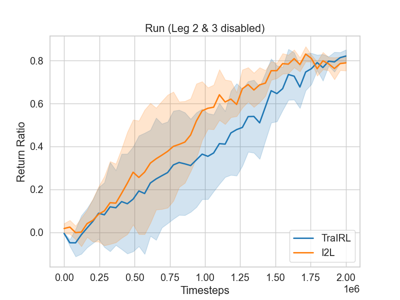
(b) Training curve in Ant (Leg 2 & 3).

Figure 6: Training curve for Ant Environment including both source domains. The true cumulative reward is used here for evaluation. AIRL and $f$-IRL perform poorly in the experiments and are therefore excluded from the comparison.

References

- Allen et al. [2021] Cameron Allen, Neev Parikh, Omer Gottesman, and George Konidaris. Learning markov state abstractions for deep reinforcement learning. Advances in Neural Information Processing Systems, 34:8229–8241, 2021.
- Arjovsky et al. [2017] Martin Arjovsky, Soumith Chintala, and Léon Bottou. Wasserstein generative adversarial networks. In Doina Precup and Yee Whye Teh, editors, Proceedings of the 34th International Conference on Machine Learning, volume 70 of Proceedings of Machine Learning Research, pages 214–223. PMLR, 06–11 Aug 2017.
- Arora and Doshi [2021] Saurabh Arora and Prashant Doshi. A survey of inverse reinforcement learning: Challenges, methods and progress. Artificial Intelligence, 297:103500, 2021.
- Cao et al. [2024] Haoyang Cao, Samuel N. Cohen, and Łukasz Szpruch. Identifiability in inverse reinforcement learning. In Proceedings of the 35th International Conference on Neural Information Processing Systems, NIPS ’21, Red Hook, NY, USA, 2024. Curran Associates Inc.
- Erickson et al. [2019] Zackory Erickson, Vamsee Gangaram, Ariel Kapusta, C. Karen Liu, and Charles C. Kemp. Assistive gym: A physics simulation framework for assistive robotics. CoRR, abs/1910.04700, 2019.
- Finn et al. [2016] Chelsea Finn, Sergey Levine, and Pieter Abbeel. Guided cost learning: Deep inverse optimal control via policy optimization. In International conference on machine learning, pages 49–58. PMLR, 2016.
- Fu et al. [2018] Justin Fu, Katie Luo, and Sergey Levine. Learning robust rewards with adverserial inverse reinforcement learning. In International Conference on Learning Representations, 2018.
- Gangwani and Peng [2020] Tanmay Gangwani and Jian Peng. State-only imitation with transition dynamics mismatch. In 8th International Conference on Learning Representations, ICLR 2020, Addis Ababa, Ethiopia, April 26-30, 2020. OpenReview.net, 2020.
- Garg et al. [2021] Divyansh Garg, Shuvam Chakraborty, Chris Cundy, Jiaming Song, and Stefano Ermon. Iq-learn: Inverse soft-q learning for imitation. Advances in Neural Information Processing Systems, 34:4028–4039, 2021.
- Gauss and Davis [1857] Carl Friedrich Gauss and Charles Henry Davis. Theory of the motion of the heavenly bodies moving about the sun in conic sections. Gauss’s Theoria Motus, 76(1):5–23, 1857.
- Ghasemipour et al. [2020] Seyed Kamyar Seyed Ghasemipour, Richard Zemel, and Shixiang Gu. A divergence minimization perspective on imitation learning methods. In Conference on robot learning, pages 1259–1277. PMLR, 2020.
- Gulrajani et al. [2017] Ishaan Gulrajani, Faruk Ahmed, Martin Arjovsky, Vincent Dumoulin, and Aaron Courville. Improved training of wasserstein gans. In Proceedings of the 31st International Conference on Neural Information Processing Systems, NIPS’17, page 5769–5779, Red Hook, NY, USA, 2017. Curran Associates Inc.
- Haarnoja et al. [2018] Tuomas Haarnoja, Aurick Zhou, Pieter Abbeel, and Sergey Levine. Soft actor-critic: Off-policy maximum entropy deep reinforcement learning with a stochastic actor. In International conference on machine learning, pages 1861–1870. PMLR, 2018.
- Herman et al. [2016] Michael Herman, Tobias Gindele, Jörg Wagner, Felix Schmitt, and Wolfram Burgard. Inverse reinforcement learning with simultaneous estimation of rewards and dynamics. In Artificial intelligence and statistics, pages 102–110. PMLR, 2016.
- Ho and Ermon [2016] Jonathan Ho and Stefano Ermon. Generative adversarial imitation learning. Advances in neural information processing systems, 29, 2016.
- Kang et al. [2024] Yachen Kang, Jinxin Liu, and Donglin Wang. Off-dynamics inverse reinforcement learning. IEEE Access, 2024.
- Kim et al. [2021] Kuno Kim, Shivam Garg, Kirankumar Shiragur, and Stefano Ermon. Reward identification in inverse reinforcement learning. In Marina Meila and Tong Zhang, editors, Proceedings of the 38th International Conference on Machine Learning, volume 139 of Proceedings of Machine Learning Research, pages 5496–5505. PMLR, 18–24 Jul 2021.
- Kingma and Welling [2014] Diederik P. Kingma and Max Welling. Auto-encoding variational bayes. In Yoshua Bengio and Yann LeCun, editors, 2nd International Conference on Learning Representations, ICLR 2014, Banff, AB, Canada, April 14-16, 2014, Conference Track Proceedings, 2014.
- Lagrange [1788] Joseph-Louis Lagrange. Mécanique Analytique. Desaint, Paris, 1788.
- Lee et al. [2019] Lisa Lee, Benjamin Eysenbach, Emilio Parisotto, Eric P. Xing, Sergey Levine, and Ruslan Salakhutdinov. Efficient exploration via state marginal matching. CoRR, abs/1906.05274, 2019.
- Mendez et al. [2018] Jorge Mendez, Shashank Shivkumar, and Eric Eaton. Lifelong inverse reinforcement learning. Advances in neural information processing systems, 31, 2018.
- Ng and Russell [2000] Andrew Y. Ng and Stuart Russell. Algorithms for inverse reinforcement learning. In Pat Langley, editor, Proceedings of the Seventeenth International Conference on Machine Learning (ICML 2000), Stanford University, Stanford, CA, USA, June 29 - July 2, 2000, pages 663–670. Morgan Kaufmann, 2000.
- Ni et al. [2021] Tianwei Ni, Harshit Sikchi, Yufei Wang, Tejus Gupta, Lisa Lee, and Ben Eysenbach. f-irl: Inverse reinforcement learning via state marginal matching. In Conference on Robot Learning, pages 529–551. PMLR, 2021.
- Ramachandran and Amir [2007] Deepak Ramachandran and Eyal Amir. Bayesian inverse reinforcement learning. In IJCAI, volume 7, pages 2586–2591, 2007.
- Rolland et al. [2022] Paul Rolland, Luca Viano, Norman Schürhoff, Boris Nikolov, and Volkan Cevher. Identifiability and generalizability from multiple experts in inverse reinforcement learning. Advances in Neural Information Processing Systems, 35:550–564, 2022.
- Rolland et al. [2024] Paul Rolland, Luca Viano, Norman Schürhoff, Boris Nikolov, and Volkan Cevher. Identifiability and generalizability from multiple experts in inverse reinforcement learning. In Proceedings of the 36th International Conference on Neural Information Processing Systems, NIPS ’22, Red Hook, NY, USA, 2024. Curran Associates Inc.
- Schlaginhaufen and Kamgarpour [2024] Andreas Schlaginhaufen and Maryam Kamgarpour. Towards the transferability of rewards recovered via regularized inverse reinforcement learning. CoRR, abs/2406.01793, 2024.
- Schulman et al. [2016] John Schulman, Philipp Moritz, Sergey Levine, Michael I. Jordan, and Pieter Abbeel. High-dimensional continuous control using generalized advantage estimation. In Yoshua Bengio and Yann LeCun, editors, 4th International Conference on Learning Representations, ICLR 2016, San Juan, Puerto Rico, May 2-4, 2016, Conference Track Proceedings, 2016.
- Sengadu Suresh et al. [2023] Prasanth Sengadu Suresh, Yikang Gui, and Prashant Doshi. Dec-airl: Decentralized adversarial irl for human-robot teaming. In Proceedings of the 2023 International Conference on Autonomous Agents and Multiagent Systems, pages 1116–1124, 2023.
- Tanwani and Billard [2013] Ajay Kumar Tanwani and Aude Billard. Transfer in inverse reinforcement learning for multiple strategies. In 2013 IEEE/RSJ International Conference on Intelligent Robots and Systems, pages 3244–3250, 2013.
- Todorov et al. [2012] Emanuel Todorov, Tom Erez, and Yuval Tassa. Mujoco: A physics engine for model-based control. In 2012 IEEE/RSJ International Conference on Intelligent Robots and Systems, pages 5026–5033, 2012.
- Van der Maaten and Hinton [2008] Laurens Van der Maaten and Geoffrey Hinton. Visualizing data using t-sne. Journal of machine learning research, 9(11), 2008.
- Viano et al. [2024] Luca Viano, Yu-Ting Huang, Parameswaran Kamalaruban, Adrian Weller, and Volkan Cevher. Robust inverse reinforcement learning under transition dynamics mismatch. In Proceedings of the 35th International Conference on Neural Information Processing Systems, NIPS ’21, Red Hook, NY, USA, 2024. Curran Associates Inc.
- Yoo and Seo [2022] Se-Wook Yoo and Seung-Woo Seo. Learning multi-task transferable rewards via variational inverse reinforcement learning. In 2022 International Conference on Robotics and Automation (ICRA), pages 434–440. IEEE, 2022.
- Yu et al. [2019] Lantao Yu, Tianhe Yu, Chelsea Finn, and Stefano Ermon. Meta-inverse reinforcement learning with probabilistic context variables. Advances in neural information processing systems, 32, 2019.
- Zakka et al. [2022] Kevin Zakka, Andy Zeng, Pete Florence, Jonathan Tompson, Jeannette Bohg, and Debidatta Dwibedi. Xirl: Cross-embodiment inverse reinforcement learning. In Conference on Robot Learning, pages 537–546. PMLR, 2022.
- Zhuang et al. [2021] Fuzhen Zhuang, Zhiyuan Qi, Keyu Duan, Dongbo Xi, Yongchun Zhu, Hengshu Zhu, Hui Xiong, and Qing He. A comprehensive survey on transfer learning. Proc. IEEE, 109(1):43–76, 2021.
- Ziebart et al. [2010] Brian D. Ziebart, J. Andrew Bagnell, and Anind K. Dey. Modeling interaction via the principle of maximum causal entropy. In Proceedings of the 27th International Conference on International Conference on Machine Learning, ICML’10, page 1255–1262, Madison, WI, USA, 2010. Omnipress.