A Heavily Right Strategy for Integrating Dependent Studies in Any Dimension

Abstract

Recently, there has been a surge of interest in hypothesis testing methods for combining dependent studies without explicitly assessing their dependence. Among these, the Cauchy combination test (CCT) stands out for its approximate validity and power, leveraging a heavy-tail approximation insensitive to dependence. However, CCT is highly sensitive to large $p$-values and inverting it to construct confidence regions can result in regions lacking compactness, convexity, or connectivity. This article proposes a “heavily right” strategy by excluding the left half of the Cauchy distribution in the combination rule, retaining CCT’s resilience to dependence while resolving its sensitivity to large $p$-values. Moreover, the Half-Cauchy combination as well as the harmonic mean approach guarantees bounded and convex confidence regions, distinguishing them as the only known combination tests with all such desirable properties. Efficient and accurate algorithms are introduced for implementing both methods. Additionally, we develop a divide-and-combine strategy for constructing confidence regions for high-dimensional mean estimation using the Half-Cauchy method, and empirically illustrate its advantages over the Hotelling $T^{2}$ approach. To demonstrate the practical utility of our Half-Cauchy approach, we apply it to network meta-analysis, constructing simultaneous confidence intervals for treatment effect comparisons across multiple clinical trials.

1 Dependence-Resilient Inference

1.1 Addressing Dependence: Three Classes of Approaches

In any theoretical or empirical investigation involving multiple entities—whether individual subjects, their characteristics, or studies related to them—assessing and accounting for their mutual influence is a key marker of scientific rigor. Conversely, a purely atomistic approach to analyzing multiple entities without valid justification often raises concerns about the credibility of the results. In statistical studies, stochastic dependence encapsulates these interrelationships, making it essential for statistical validity. Realistically assessing dependence, however, is challenging, especially in high-dimensional settings, as it requires substantial data and information to ensure reliability. Numerous methods have been proposed to address stochastic dependence, and most fall into two broad categories (see Appendix˜F).

• Simplistic Assertive Approaches rely on strong assumptions to simplify dependence structures, such as assuming independencies or equal correlations.

  • Pros: Greatly simplified modeling and computation, making them more generally accessible.

  • Cons: Great risk of inaccuracies and challenges in scientific justification.

• Model-Intensive Approaches employ data-driven methods to estimate pre-specified dependence structures, relying on more flexible and realistic assumptions compared to the assertive approaches.

  • Pros: More principled approach with stronger validity and efficiency.

  • Cons: Greater modeling and computational demand, and higher risk of overfitting.

Recently, a third class of methods has gained considerable attention, which we categorize as dependence-resilient approaches because their validity is robust to dependence beyond what is specified by the model.

• Dependence-Resilient Approaches construct tests or estimates that are insensitive to dependence.

  • Pros: Principled and easy to apply, compute, and interpret.

  • Cons: Can be overly conservative, without careful constructions.

Traditionally, approaches in this third category, such as Bonferroni correction, are not desirable because of their overly conservative nature, especially in high dimensions. The development of dependence-resilient approaches with acceptable power began about a decade ago, largely motivated by a surprising observation made by Drton and Xiao [2016].

1.2 A Cauchy Surprise and Its “Afterstat”

Let $\boldsymbol{X}=(X_{1},\ldots,X_{m})^{\top}$ and $\boldsymbol{Y}=(Y_{1},\ldots,Y_{m})^{\top}$ be two independent samples from $\mathcal{N}(\boldsymbol{0},\boldsymbol{\Sigma})$, where $\boldsymbol{\Sigma}>0$ is $m\times m$. Based on simulations, Drton and Xiao [2016] conjectured that for any $\boldsymbol{w}=\{w_{1},\ldots,w_{m}\}$ with $\sum_{j=1}^{m}w_{j}=1$,

$$\small\normalsize T_{\boldsymbol{w}}=\sum_{j=1}^{m}w_{j}\frac{X_{j}}{Y_{j}}\sim\text{Cauchy}(0,1)\quad[\text{Cauchy distribution with center 0 and scale 1}],\small\normalsize$$ (1.1)

as long as $w_{j}\geq 0$. They provided a proof for $m=2$, and left it as a conjecture for general $m>2$.

When $\boldsymbol{\Sigma}$ is not diagonal, the ratios $X_{j}/Y_{j}$ (for $j=1,\ldots,m$)—although each individually Cauchy distributed—are not independent. Therefore, it seems too good to be true that their weighted sum also follows Cauchy(0,1) exactly, regardless of $\boldsymbol{\Sigma}>0$. However, Pillai and Meng [2016] proved that (1.1) indeed holds for arbitrary $m$, based on a largely forgotten result that apparently generated the “afterstat” of this Cauchy surprise. Specifically, for any $\{u_{1},\ldots,u_{m}\}$, where $u_{j}\in\mathbb{R}$, and $\Theta_{1}\sim\text{Unif}(-\pi,\pi]$ independent of $\{w_{1},\ldots,w_{m}\}$ where $w_{j}\geq 0$ and $\sum_{j}w_{j}=1$, Williams [1969] reports that

$$\small\normalsize\sum_{j=1}^{m}w_{j}\tan(\Theta_{1}+u_{j})\sim\text{Cauchy}(0,1).\small\normalsize$$ (1.2)

Writing $\{X_{j}=R_{j}\cos(\Theta_{j}),Y_{j}=R_{j}\sin(\Theta_{j})\}$ and proving $\{u_{i}=(\Theta_{j}-\Theta_{1}),\mod(2\pi),j=2,\ldots,m\}$ is independent of $\Theta_{1}$ under the normal model, Pillai and Meng [2016] establishes (1.1) because $T_{\boldsymbol{w}}=\sum_{j=1}^{m}w_{j}\tan(\Theta_{1}+u_{j})$.

The result in (1.1) has found applications in a variety of fields, from financial portfolio management [Lindquist and Rachev 2021] to genomewide epigenetic studies [Liu et al. 2022], and to understanding post-processing noise in differentially private wireless federated learning [Wei et al. 2023]. It also prompted theoretical work on heavy tail distributions [Cohen et al. 2020; Xu et al. 2022], as well as suggested the existence of useful statistics that are ancillary to the dependence structure, giving rise to the potential power of Cauchy combination rules. In particular, Liu and Xie [2020] proposed combining $m$ possibly correlated $p$-values $\{p_{1},\ldots,p_{m}\}$ for testing the same null hypothesis $H_{0}$ via

$$\small\normalsize T_{\text{CCT}}=\sum_{j=1}^{m}w_{j}\tan\bigl{\{}(1/2-p_{j})\pi\bigr{\}}=\sum_{j=1}^{m}w_{j}\cot(p_{j}\pi).\small\normalsize$$ (1.3)

The power of (1.3) is also demonstrated in the highly cited paper by Liu et al. [2019] for using CCT in rare-variant analysis.

The same tangent function combining rule adopted by (1.3) and (1.2) hints at the potential dependence resilience nature of $T_{\text{CCT}}$. Indeed, as Liu and Xie [2020] demonstrated, under mild dependence assumptions, $T_{\text{CCT}}$ exhibits a Cauchy-like tail behavior. Specifically, they represented $p_{j}=2\{1-\Phi(|Z_{j}|)\}$, where $\Phi(z)$ is the CDF of $\mathcal{N}(0,1)$. If for any $i\neq j$, $(Z_{i},Z_{j})$ are bivariate normal with mean zero and mild constraints on $\boldsymbol{\Sigma}$, the covariance matrix of $(Z_{1},\ldots,Z_{p})$, then

$$\small\normalsize\lim_{t\rightarrow\infty}\frac{\mathbb{P}(T_{\text{CCT}}\geq t)}{\mathbb{P}(C\geq t)}=1,\quad{\text{where}}\quad C\sim\text{Cauchy}(0,1).\small\normalsize$$ (1.4)

Subsequently, Vovk and Wang [2020], Vovk et al. [2022], and Fang et al. [2023] showed that such robustness against dependence in $\boldsymbol{\Sigma}$ can be extended to other combination methods, such as the harmonic mean $p$-value (HMP) $T_{\text{HMP}}=\sum_{j=1}^{m}w_{j}/p_{j}$ [Good 1958; Wilson 2019]. A commonality of these methods is the use of quantile functions from heavy-tailed distributions—$\cot(p\pi)$ for Cauchy and $1/p$ for $\text{Pareto}(1,1)$—to transform individual $p$-values before combining them. The stability of Cauchy facilitates tracking of the null distribution for independent studies, and inspires extensions such as the Lévy and stable combination tests via other stable distributions [Wilson 2021; Ling and Rho 2022].

1.3 A Heavily Right Strategy

Because $\tan(x)$ approaches $-\infty$ when $x\downarrow-\pi/2$, the CCT statistic in (1.3) will approach $-\infty$ even if only one $p_{j}$ approaches 1 (and none of the $p_{i}$’s is extremely significant to compensate). This extreme sensitivity to large $p$-values is undesirable theoretically and practically [Fang et al. 2023]. For example, in genome-wide association studies, only a few SNPs (Single Nucleotide Polymorphisms) are likely related to the phenotype of interest, with most $p$-values close to one [Zeggini and Ioannidis 2009]. In such cases, CCT can cause numerical instability and substantial power loss.

Another limitation of CCT and similar methods is that inverting the global test does not always yield reasonable confidence regions. If we aim to obtain a confidence set for a parameter $\boldsymbol{\theta}$ by inverting a CCT based on multiple studies—each testing $H_{0}:\boldsymbol{\theta}=\boldsymbol{\theta}_{0}$ against $H_{1}:\boldsymbol{\theta}\neq\boldsymbol{\theta}_{0}$—the acceptance region for $\boldsymbol{\theta}_{0}$ may be non-convex or even disconnected, as illustrated in the following two examples.

1. Suppose we have two equally weighted studies with estimators from $\mathcal{N}(\theta_{0},0.01)$ and obtain estimates of $0.125$ and $-0.125$. Inverting CCT at a $5\%$ significance level yields a disconnected $95\%$ confidence set: $[-0.1277,-0.1212]\cup[-0.1038,0.1038]\cup[0.1212,0.1277]$, which includes the two individual estimates, as illustrated in Figure˜1(a).

2. Suppose that we have three equally weighted studies with estimators from $\mathcal{N}(\boldsymbol{\theta}_{0},0.01\boldsymbol{I}_{2})$, and obtain estimates $(-0.10,-0.10)$, $(0.21,0)$, and $(0,0.21)$. Inverting CCT at a $5\%$ significance level yields disconnected $95\%$ confidence regions, which include all three individual estimates, as shown in Figure˜1(b).

Later in Section˜3.3, we will explain why any CCT region necessarily includes all individual estimates, irrespective of the confidence levels. This undesirable property, recognized in Meng [2024], along with other defects of inverting CCT for constructing confidence regions, serves as a springboard for the present article.

Specifically, to address the limitations of CCT, we propose a heavily right strategy by replacing the Cauchy distribution with a Half-Cauchy (HC) distribution when transforming p-values into scores. This approach, termed the Half-Cauchy Combination Test (HCCT), reflects the HC distribution’s heavy right tail and the absence of a left tail. This heavily right strategy effectively resolves the two limitations of CCT revealed earlier, as demonstrated in Figures˜1(a) and 1(b). However, it introduces a computational challenge, because the HC distribution, unlike the Cauchy distribution, is not a stable distribution. To overcome this, we develop a new approach to compute exact tail probabilities for HCCT scores with a finite number of independent studies, leveraging Laplace transforms and numerical integration.

(a)

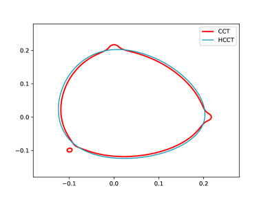
(b)

Figure 1: Connectivity of confidence regions for CCT and HCCT.

Concurrent research explored left-truncated or winsorized Cauchy methods to reduce sensitivity to large $p$-values [Gui et al. 2023; Fang et al. 2023], and our HC method is a special case of the left-truncation. However, these previous approaches did not provide sufficiently accurate distribution calculations for the test statistic, even with independent studies (see Table˜2), which undermined the validity of these methods. Furthermore, they did not address the challenge of constructing confidence regions for parameter estimation. In fact, we show that HC is the only distribution in their proposed family of methods that guarantees connected confidence regions (see Section˜3).

Another notable dependence-resilient approach for global testing is the harmonic mean $p$-value (HMP) mentioned earlier, which has been generalized to other averaging techniques [Vovk and Wang 2020; Fang et al. 2023], with a high-level theoretical analysis of this class provided by Vovk et al. [2022]. We show that HMP is not sensitive to large $p$-values and produces connected confidence regions, because the underlying quantile function is from Pareto$(1,1)$, which also has a heavy right tail without a left tail, similar to HC. Inspired by our numerical approach for HCCT, we provide a similar method for computing the exact null distribution of HMP for a finite number of independent studies, allowing for flexible weights. This approach, EHMP (Exact Harmonic Mean $p$-value), reduces the computational defects with HMP.

		Validity (dependent tests)	Power (dependent tests)	Exactness (independent tests)	Insensitivity to large $p$-values	Convexity of confidence regions
Fisher [Fisher 1925]		[][red]	[][green]	[][green]	[][green]	[][yellow]
Stouffer [Stouffer et al. 1949]		[][red]	[][green]	[][green]	[][red]	[][red]
Bonferroni [Dunn 1961]		[][green]	[][red]	[][red]	[][green]	[][green]
Simes [Simes 1986]		[][green]	[][red]	[][red]	[][green]	[][green]
HMP [Good 1958; Wilson 2019]		[][green]	[][green]	[][red]	[][green]	[][green]
CCT [Liu and Xie 2020]		[][green]	[][green]	[][green]	[][red]	[][red]
LCT [Wilson 2021]		[][green]	[][red]	[][green]	[][green]	[][red]
SCT [Ling and Rho 2022]	$\alpha<1$	[][green]	[][red]	[][green]	[][green]	[][red]
	$\alpha>1$	[][red]	[][green]	[][green]	[][green]	[][red]
CAtr [Fang et al. 2023]		[][green]	[][green]	[][yellow]	[][yellow]	[][red]
Left-Truncated $t$ [Gui et al. 2023]	$\alpha<1$	[][green]	[][red]	[][red]	[][yellow]	[][red]
	$\alpha=1$	[][green]	[][green]	[][red]	[][yellow]	[][red]
	$\alpha>1$	[][red]	[][green]	[][red]	[][yellow]	[][red]
HCCT [Proposed]		[][green]	[][green]	[][green]	[][green]	[][green]
EHMP [Proposed]		[][green]	[][green]	[][green]	[][green]	[][green]

Table 1: Comparison of different combination tests. The smiley (green), stoic (yellow), and sad (red) faces represent respectively positive, neutral, and negative rating. HMP is shorthand for Harmonic Mean P-value; CCT for Cauchy Combination Test; LCT for Lévy Combination Test; SCT for Stable Combination Test; CAtr for CAuchy with truncation; HCCT for Half-Cauchy Combination Test; EHMP for Exact Harmonic Mean P-value.

1.4 Summary of Findings and Contributions

Table˜1 previews the comparisons of various testing methods that will be discussed in our article, highlighting their pros and cons. Specifically, Fisher’s combination test, Stouffer’s Z-score test, and Stable Combination Test (SCT) and Left-Truncated $t$ with the stability parameter $\alpha>1$ tend to have inflated Type I error rates under dependence, while methods like the Bonferroni correction, Simes’ test, Lévy Combination Test (LCT), and SCT and Left-Truncated $t$ with $\alpha<1$ are overly conservative. The majority of previous methods (including Left-Truncated $t$ approaches when not truncated at zero) do not guarantee connected confidence regions, and some are highly sensitive to large $p$-values. In contrast, the two heavily right approaches we proposed, namely HCCT and EHMP, perform well across all these criteria.

The rest of the paper is organized as follows. Section˜2 introduces HCCT as an example of the heavily right strategy, and examines its properties; the corresponding results for EHMP are deferred to the supplemental material (Appendix˜A) to save space. Section˜3 then inverts HCCT to obtain confidence regions, establishes their convexity and compactness in common scenarios, and presents algorithms for computing them.

To demonstrate the potential of our approach, Section˜4 proposes a divide-and-combine strategy for high-dimensional mean estimation, providing a variety of set estimators that generalize Hotelling’s $T^{2}$ approach. Notably, this strategy does not require estimating the full covariance matrix or even any matrix and can yield potentially more compact confidence regions with valid coverage. Section˜5 examines the competitiveness of our approach to network meta-analysis in clinical trials, using both semi-synthetic and real-data examples.

The concluding Section˜6 explicates practical limitations and theoretical open problems of our current proposals, which we hope will serve as a warm invitation to the statistical and broader data science community to fully explore and leverage the paradigm of heavy-tail approximation refined by the heavily-right strategy, just as we have for the large-sample approximations with a host of refinements throughout the history of statistical inference. Details on EHMP, further analysis of HCCT, and all proofs are in the supplemental material [Liu et al. 2024], so is a section that briefly reviews the literature on other global testing procedures that are not necessarily dependence-resilient.

2 Half-Cauchy Combination Tests

2.1 A General Strategy for Combining $p$-Values and the Roles of Stable Distributions

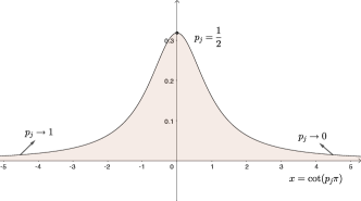
(a)

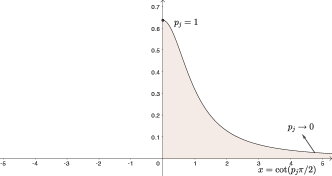
(b)

Figure 2: Cauchy vs Half-Cauchy.

Let $p_{j},j=1,2,\dots,m$ be individual $p$-values from hypothesis tests for a common null hypothesis, and our goal is to combine $p_{j}$’s into one test statistic. In general, given a random variable $\nu$ on $\mathbb{R}$ with CDF $F_{\nu}(x)$, we consider the following

$$\small\normalsize\textstyle T_{\nu,\boldsymbol{w}}=\sum_{j=1}^{m}w_{j}F_{\nu}^{-1}(1-p_{j}),\quad\text{where }\sum_{j=1}^{m}w_{j}=1,\quad w_{j}\geq 0\quad\forall j=1,\dots,m.\small\normalsize$$ (2.1)

If $p_{j}$’s are uniformly distributed between $0$ and $1$, then $F^{-1}_{\nu}(1-p_{j})$’s are identically distributed as $\nu$. Many choices are made in the literature, such as $\nu\sim\chi_{2}^{2}$ by Fisher’s method and $\nu\sim\mathcal{N}(0,1)$ for Stouffer’s Z-score method. For HMP $\nu\sim{\textup{Pareto}}(1,1)$ with density given by $f_{\nu}(x)={x^{-2}}\mathbb{I}_{x\geq 1}$, and for CCT $\nu\sim{\textup{Cauchy}}(0,1)$. Consequently,

$$\small\normalsize\textstyle T_{\textup{HMP}}=\sum_{j=1}^{m}\frac{w_{j}}{p_{j}},\quad T_{\textup{CCT}}=\sum_{j=1}^{m}w_{j}\cot(p_{j}\pi).\small\normalsize$$ (2.2)

As illustrated in Figure˜2, replacing Cauchy by Half-Cauchy defines our HC combination statistic

$$\small\normalsize\textstyle T_{\textup{HCCT}}=\sum_{j=1}^{m}w_{j}F^{-1}_{\mathrm{HC}}(1-p_{j})=\sum_{j=1}^{m}w_{j}\cot\Bigl{(}\frac{p_{j}\pi}{2}\Bigr{)}.\small\normalsize$$ (2.3)

To examine its asymptotic properties with $m\to\infty$, we need a few basic concepts from extreme value theory. A distribution is called stable if any linear combination of two independent random variables from this distribution results in a variable that has the same distribution, up to location and scale transformations. All continuous stable distributions $S(\alpha,\beta,c,\mu)$ can be obtained from the following parametrization of the characteristic function:

$$\small\normalsize\phi(t;\alpha,\beta,c,\mu)=\exp\bigl{[}it\mu-\lvert ct\rvert^{\alpha}\bigl{\{}1-i\beta\operatorname{sgn}(t)\chi(\alpha,t)\bigr{\}}\bigr{]},\quad\text{with}\quad\chi(\alpha,t)=\begin{cases}\tan\Bigl{(}\frac{\pi\alpha}{2}\Bigr{)}&\text{if }\alpha\neq 1\\ -\frac{2}{\pi}\log\lvert t\rvert&\text{if }\alpha=1\end{cases},\small\normalsize$$

where $\operatorname{sgn}(t)$ is the sign of $t$. Here $\alpha\in(0,2]$ is the stability parameter that controls the tail of the distribution, $\beta\in[-1,1]$ is called the skewness parameter, $c\in(0,\infty)$ is the scale, and $\mu\in(-\infty,\infty)$ is the location parameter. Except for the normal distribution ($\alpha=2$), the stable family is always heavy-tailed. In particular, $\alpha=1$ and $\beta=0$ results in the Cauchy distribution, and $\alpha=\beta=1$ defines the Landau family [Zolotarev 1986] with the density function

$$\small\normalsize\textstyle f_{\textup{Landau}}(x;\mu,c)=\frac{1}{c\pi}\int_{0}^{\infty}\exp(-t)\cos\Bigl{\{}\frac{(x-\mu)t}{c}+\frac{2}{\pi}t\log\frac{t}{c}\Bigr{\}}\mathop{}\!\mathrm{d}t.\small\normalsize$$

2.2 Half-Cauchy is Attracted to Landau

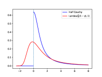
(a)

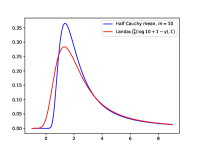
(b)

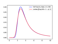
(c)

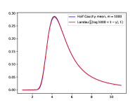
(d)

Figure 3: Density functions for Landau distribution and Half-Cauchy means.

Let $X_{1},X_{2},\dots,X_{n}$ be a sequence of random variables i.i.d. from $\nu$. If for suitably chosen real-number sequences $A_{n}$ and $B_{n}$, $\textstyle B_{n}^{-1}\sum_{i=1}^{n}X_{i}-A_{n}\mathrel{\xrightarrow{\textup{d}}}\mathcal{L},$ we say that $\nu$ is attracted to the limiting distribution $\mathcal{L}$. The totality of distributions attracted to $\mathcal{L}$ is called the domain of attraction of $\mathcal{L}$. A key result is that only stable distributions have non-empty domains of attraction and each stable distribution $S(\alpha,\beta,c,\mu)$ with different values of $\alpha$ or $\beta$ (except when $\alpha=2$) has a distinct domain of attraction [Gnedenko and Kolmogorov 1954]. For more references on this notion and the generalized central limit theorem, see Zolotarev [1986], Uchaikin and Zolotarev [2011], and Shintani and Umeno [2018].

We show that the standard HC lies in the domain of attraction of $\textup{Landau}(0,1)$:

Theorem 2.1.

Consider a triangular array of non-negative weights $\{w_{j}^{(m)},1\leq j\leq m;m\geq 1\}$, such that $\sum_{j=1}^{m}w_{j}^{(m)}=1$ for any $m\geq 1$ and that $\max_{j}w_{j}^{(m)}\to 0$ as $m\to\infty$. Let $\{X_{j},j=1,\ldots\}$ be a sequence of i.i.d. variables from standard Half-Cauchy, then we have

$$\small\normalsize\sum_{j=1}^{m}w_{j}^{(m)}X_{j}-\frac{2}{\pi}\Bigl{\{}-\sum_{j=1}^{m}w_{j}^{(m)}\log w_{j}^{(m)}+1-\gamma\Bigr{\}}\mathrel{\xrightarrow{\textup{d}}}S(1,1,1,0)=\textup{Landau}(0,1),\small\normalsize$$

where $\gamma=\lim_{m\to\infty}\Bigl{(}\sum_{k=1}^{m}\frac{1}{k}-\log m\Bigr{)}\approx 0.5772$ is the Euler–Mascheroni constant [Campbell 2003].

To gain intuition from Theorem˜2.1, Figure˜3 provides the density comparison between weighted HC sums and their Landau approximations. The Landau distribution is supported on $\mathbb{R}$ but its negative tail decays so fast that it is negligible. The following proposition of Zolotarev [1986] provides the stability property of Landau distributions:

Proposition 2.2.

If $X\sim\textup{Landau}(\mu,c)$, then $aX+b\sim\textup{Landau}\Bigl{(}a\mu+b-\frac{2c}{\pi}a\log a,ac\Bigr{)}$ for any $a>0$. If $X\sim\textup{Landau}(\mu_{1},c_{1})\mathrel{\hbox to0.0pt{$\perp$\hss}{\kern 2.0pt\perp}}Y\sim\textup{Landau}(\mu_{2},c_{2})$, then $X+Y\sim\textup{Landau}(\mu_{1}+\mu_{2},c_{1}+c_{2})$.

A caveat is that the Landau distribution is not strictly stable in the sense that the location parameter does not change proportionally with rescaling. For example, if $X_{1},\dots,X_{m}$ is i.i.d. $\textup{Landau}(\mu,1)$, then we can check that

$$\small\normalsize\textstyle\sum_{j=1}^{m}w_{j}X_{j}\sim\textup{Landau}(-\frac{2}{\pi}\sum_{j=1}^{m}w_{j}\log w_{j}+\mu,1).\small\normalsize$$

2.3 Numerical Computation

Theorem˜2.1 hints that, unlike a weighted sum of independent Cauchy variables, which retains the Cauchy distribution, a weighted sum of independent HC variables is not well-characterized. Fortunately, we are able derive its density and CDF, which enables us to provide an efficient and precise numerical method for computing its density, CDF, and quantile function. The same approach can be adapted to calculate these functions for HMP (see Appendix˜A).

Define the sine integral $\operatorname{si}(z)$ and cosine integral $\operatorname{ci}(z)$ [Abramowitz and Stegun 1968] by

$$\small\normalsize\textstyle\operatorname{si}(z)=-\int_{z}^{\infty}\frac{\sin(\xi)}{\xi}\mathop{}\!\mathrm{d}\xi,\qquad\operatorname{ci}(z)=\int_{z}^{\infty}\frac{\cos(\xi)}{\xi}\mathop{}\!\mathrm{d}\xi,\qquad z>0.\small\normalsize$$ (2.4)

Then the Laplace transform of $f_{\mathrm{HC}}(x)$ can be expressed as

$$\small\normalsize\textstyle f_{\textup{HC}}^{\ast}(z)=\frac{2}{\pi}\int_{0}^{+\infty}\frac{\exp(-xz)}{1+x^{2}}\mathop{}\!\mathrm{d}x=-\frac{2}{\pi}\{\sin(z)\operatorname{ci}(z)+\cos(z)\operatorname{si}(z)\}.\small\normalsize$$

Theorem 2.3.

For i.i.d. Half-Cauchy $\{X_{1},\ldots,X_{m}\}$, the density and CDF of $\sum_{j=1}^{m}w_{j}X_{j}$ can be expressed respectively as

$$\begin{aligned} f_{\textup{HC},\boldsymbol{w}}(x)=&\textstyle\frac{1}{2\pi i}\int_{0}^{\infty}\exp(-xz)\Bigl{[}\prod_{j=1}^{m}\{-f^{\ast}(w_{j}z)+2\cos(w_{j}z)+2i\sin(w_{j}z)\}\\ &\textstyle-\prod_{j=1}^{m}\{-f^{\ast}(w_{j}z)+2\cos(w_{j}z)-2i\sin(w_{j}z)\}\Bigr{]}\mathop{}\!\mathrm{d}z,\end{aligned}$$ (2.5)

$$\begin{aligned} F_{\textup{HC},\boldsymbol{w}}(x)=&\textstyle 1-\frac{1}{2\pi i}\int_{0}^{\infty}\frac{\exp(-xz)}{z}\Bigl{[}\prod_{j=1}^{m}\{-f^{\ast}(w_{j}z)+2\cos(w_{j}z)+2i\sin(w_{j}z)\}\\ &\textstyle-\prod_{j=1}^{m}\{-f^{\ast}(w_{j}z)+2\cos(w_{j}z)-2i\sin(w_{j}z)\}\Bigr{]}\mathop{}\!\mathrm{d}z.\end{aligned}\small\normalsize$$ (2.6)

While computing $f_{\textup{HC},\boldsymbol{w}}(x)$ or $F_{\textup{HC},\boldsymbol{w}}(x)$ using Theorem 2.3, the numerical integration is performed only once and the integrand in (2.5) and (2.6) can be computed in linear time with respect to $m$. The complex number operations are natively supported by the Python package NumPy, and both sine and cosine integrals are available as predefined special functions in SciPy. To maintain accuracy and prevent overflow, we employ the logarithmic transformation to convert products into summations in the implementation. Specifically we compute the integrand using the following formula

$$\textstyle\exp(-xz)\Bigl{[}\prod_{j=1}^{m}\{-f^{\ast}(w_{j}z)+2\cos(w_{j}z)+2i\sin(w_{j}z)\}-\prod_{j=1}^{m}\{-f^{\ast}(w_{j}z)+2\cos(w_{j}z)-2i\sin(w_{j}z)\}\Bigr{]}$$

$$= \textstyle 2i\operatorname{Im}\Bigl{[}\exp(-xz)\prod_{j=1}^{m}\{-f^{\ast}(w_{j}z)+2\cos(w_{j}z)+2i\sin(w_{j}z)\}\Bigr{]}$$

$$= \textstyle 2i\operatorname{Im}\exp\Bigl{[}-xz+\sum_{j=1}^{m}\log\{-f^{\ast}(w_{j}z)+2\cos(w_{j}z)+2i\sin(w_{j}z)\}\Bigr{]},$$

where $\log z$ is the complex logarithmic function on $\mathbb{C}\backslash\{0\}$.

Similar challenges have arisen HMP [Wilson 2019]) and the left-truncated or winsorized Cauchy method [Gui et al. 2023; Fang et al. 2023]. Wilson [2019] used the limiting Landau distribution as an approximation regardless of $m$, which proves inaccurate for small $m$. In contrast, Fang et al. [2023] introduced an iterative importance sampling scheme for small $m$, switching to the Landau approximation only when $m$ exceeds a set threshold $m_{0}$. However, this approach is computationally intensive and unstable without a very large sample size, requiring at least $10^{5}m$ samples per iteration. As a result, $m_{0}$ cannot be set too high, and they recommend $m_{0}=25$; yet, accuracy declines noticeably for $m=26$. (Consequently, we assign a neutral rating for their exactness in Table˜1. )

$m$	weights	Empirical Wilson [2019]	Oracle Wilson [2019]	Empirical Fang et al. [2023]	Oracle Fang et al. [2023]	Empirical Gui et al. [2023]	Oracle Gui et al. [2023]
2	(.5, .5)	23.57	21.73	6.33	6.32	12.71	13.69
2	(.8, .2)	23.57	21.19	6.33	6.32	12.71	13.39
5	(.2, .2, .2, .2, .2)	24.48	23.51	6.36	6.36	12.71	14.74
5	(.6, .1, .1, .1, .1)	24.48	22.64	6.36	6.37	12.71	14.24
26	(1/26, $\dots$, 1/26)	26.13	25.85	6.86	6.62	12.71	16.19

Table 2: This table shows the thresholds of $T_{\nu,\boldsymbol{w}}$ for rejecting the global null at a significance level of $0.05$. “Empirical” refers to the threshold implied by the methods in Wilson [2019]; Fang et al. [2023]; Gui et al. [2023], while “Oracle” provides the actual threshold based on the exact distribution of $T_{\nu,\boldsymbol{w}}$ for independent studies, as used in their analyses. Following recommendations from Fang et al. [2023], winsorization at the $1\%$-quantile of the Cauchy distribution is applied, and for Gui et al. [2023], left-truncation at zero is used to align with the Half-Cauchy.

$m$	$x$	PDF (Err)	Time (s)	Landau Approx (Err)	CDF (Err)	Time (s)	Landau Approx (Err)
2	.2	.292879165 ($\pm$9E-9)	.043	.282722127 ($-$2E-2)	.030804228 ($\pm$1E-8)	.028	.223733981 ($+$2E-1)
	2	.164879638 ($\pm$8E-9)	.011	.139681018 ($-$3E-2)	.639966151 ($\pm$4E-9)	.011	.621681447 ($-$2E-2)
	10	.007305301 ($\pm$5E-9)	.012	.008434884 ($+$2E-3)	.930504308 ($\pm$2E-9)	.011	.923528833 ($-$7E-3)
	50	.000267851 ($\pm$6E-9)	.006	.000282679 ($+$2E-5)	.986896089 ($\pm$3E-9)	.013	.986491736 ($-$5E-4)
10	1	.298436871 ($\pm$1E-9)	.019	.267219180 ($-$4E-2)	.084662651 ($\pm$3E-9)	.018	.161603641 ($+$8E-2)
	4	.081183591 ($\pm$9E-9)	.011	.083422558 ($+$3E-3)	.740788721 ($\pm$2E-9)	.013	.727771746 ($-$2E-2)
	10	.009975760 ($\pm$1E-9)	.012	.010582384 ($+$7E-4)	.916911594 ($\pm$4E-9)	.016	.913846326 ($-$4E-3)
	50	.000290372 ($\pm$2E-9)	.010	.000295108 ($+$5E-6)	.986315767 ($\pm$1E-9)	.014	.986195804 ($-$2E-4)
100	2	.158076048 ($\pm$4E-9)	.045	.169847092 ($+$2E-2)	.040232564 ($\pm$6E-9)	.050	.056630205 ($+$2E-2)
	5	.105381463 ($\pm$1E-9)	.021	.106135365 ($+$1E-3)	.687530806 ($\pm$1E-8)	.021	.683873904 ($-$4E-3)
	10	.015109635 ($\pm$1E-9)	.012	.015315611 ($+$3E-4)	.895973685 ($\pm$7E-9)	.017	.895170441 ($-$9E-4)
	50	.000313579 ($\pm$5E-9)	.016	.000314359 ($+$2E-6)	.985767643 ($\pm$1E-9)	.022	.985749325 ($-$2E-5)
1000	4	.277750260 ($\pm$4E-9)	.162	.274061911 ($-$4E-3)	.177916458 ($\pm$5E-9)	.185	.180088077 ($+$3E-3)
	7	.080390569 ($\pm$9E-9)	.096	.080617466 ($+$3E-4)	.733973017 ($\pm$1E-8)	.079	.733369559 ($-$6E-4)
	10	.023685955 ($\pm$2E-9)	.055	.023750783 ($+$1E-4)	.867373631 ($\pm$9E-9)	.073	.867174483 ($-$2E-4)
	50	.000335429 ($\pm$1E-8)	.068	.000335545 ($+$2E-7)	.985275813 ($\pm$2E-9)	.100	.985273239 ($-$3E-6)

Table 3: Precision and runtime cost of HCCT with equal weights, where “Err" refers to the bounds in the numerical integration, given by SciPy.

Moreover, Gui et al. [2023] directly applied the left-truncated Cauchy approximation (valid for $m=1$) to cases with $m>1$, which introduces substantial bias and undermines validity for large $m$. For a detailed comparison of the accuracy and limitations across different values of $m$ for these three approaches, see Table˜2. Furthermore, although Wilson [2019] and Fang et al. [2023] mentioned the use of importance weighting for different studies in practice, they were only able to derive the Landau approximation or compute the distribution function with equal weights for all studies. Table˜2 also shows the accuracy gap if we apply their method for unequal weights.

In contrast, our method does not rely on sampling or require equal weights, and it is significantly more efficient and precise. Table˜3 shows the computational costs, error bounds, and comparisons with Landau approximation. Since the computational cost grows linearly in $m$, we still recommend a hybrid approach that adopts the Landau approximation in Theorem˜2.1 for $m\geq 1000$. For $m<1000$, we observe that Theorem 2.3 is accurate for practical purposes; for $m=1000$, the error of approximating $F_{\textup{HC},\boldsymbol{w}}(x)$ with the Landau distribution is below $0.0002$ for $x$ larger than $90$ percentile. For computing Landau distributions, we adopted the Padé approximants; see the source code of the C++ numerical framework ROOT for implementation [Kölbig and Schorr 1983]. For further references on the computation of Landau distributions see Chambers et al. [1976]; Weron [1996]; Nolan [1997]; Teimouri and Amindavar [2008]; Ament and O’Neil [2018].

2.4 Tail Probability and Dependence-Resilient Property

Following the theoretical setup and approaches of Long et al. [2023], we establish the following theorem for HCCT.

Theorem 2.4.

Suppose that there exists a sequence of $\delta_{t}$ with $\lim\limits_{t\to\infty}\delta_{t}\to 0$ and $\lim\limits_{t\to\infty}\delta_{t}t\to\infty$ such that for some $0\leq\gamma\leq 1$

$$\small\normalsize\max_{1\leq i<j\leq m}\mathbb{P}\left(0<p_{i}<\frac{2w_{i}m}{\pi t},0<p_{j}<\frac{2w_{j}m}{\pi\delta_{t}t}\right)=o\left(\frac{1}{t^{1+\gamma}}\right),\small\normalsize$$ (2.7)

and for $\gamma>0$ the weights satisfy that $\max_{1\leq i\leq m}{w_{i}}=\mathcal{O}(1/m)$ as $m\to\infty$. Then the Half-Cauchy test statistic satisfies:

$$\small\normalsize\lim_{m=\mathcal{O}(t^{\gamma/2}),t\to\infty}\frac{\mathbb{P}(T_{\textup{HCCT}}>t)}{1-F_{\textup{HC},\boldsymbol{w}}(t)}=\lim_{m=\mathcal{O}(t^{\gamma/2}),t\to\infty}\frac{\mathbb{P}(T_{\textup{HCCT}}>t)}{1-\frac{2}{\pi}\arctan(t)}=1.\small\normalsize$$ (2.8)

Theorem˜2.4 suggests that, for a broad range of dependence structures, either $F_{\textup{HC},\boldsymbol{w}}(t)$ of (2.6) or $F_{\textup{HC}}(t)=\frac{2}{\pi}\arctan(t)$ can effectively approximate the CDF of $T_{\textup{HCCT}}$. In practice, however, when dependence is light to moderate, $F_{\textup{HC},\boldsymbol{w}}(t)$ tends to be a better approximation than $F_{\textup{HC}}(t)$. Ideally, we want the combination test to be exact or at least strictly valid for independent studies: using the rejection threshold from the inverse of $F_{\textup{HC},\boldsymbol{w}}(t)$ ensures this requirement, whereas using $F_{\textup{HC}}(t)$ slightly inflates the Type I error rate, compromising validity in the independent case. This is seen in Table˜2, where the empirical rejection threshold used in Gui et al. [2023] remains constant regardless of $m$ and is consistently lower than the oracle threshold, which actually grows logarithmically in $m$, as shown in Figure˜3.

Our assumption in Theorem˜2.4 follows from the first part of Assumption D1 in Long et al. [2023]. The second half of their assumption is not needed anymore due to the benefit of replacing Cauchy with Half-Cauchy. Interestingly, the assumption in Theorem˜2.4 can be interpreted as a weak version of tail independence for the test scores, weak because $\delta_{t}\rightarrow 0$. Intuitively, it means negligible co-movement in the tails of the score distributions for any pair of studies, which is the case for many dependent settings as enumerated in Appendix˜B. We will also provide more details on this concept and relations to previous works in Appendix˜B. In particular, any random vector that is pairwise bivariate normal with bounded correlations satisfies the assumptions in Theorem˜2.4, and thus, we have the following corollary.

Corollary 2.5.

Let $X_{1},\dots,X_{m}$ be a random vector such that for any $1\leq i,j\leq m$ the $2$-dimensional vector $(X_{i},X_{j})$ is bivariate normal with correlations given by $\rho_{ij}$ and $\mathbb{E}(X_{i})=\mu_{i}$ and $\operatorname{Var}(X_{i})=\sigma_{i}^{2}$ for $1\leq i\leq m$. Let $p_{i}$ be $1-\Phi\Bigl{(}\frac{X_{i}-\mu_{i}}{\sigma_{i}}\Bigr{)}$ (one-sided test) or $2\Bigl{\{}1-\Phi\Bigl{(}\frac{\lvert X_{i}-\mu_{i}\rvert}{\sigma_{i}}\Bigr{)}\Bigr{\}}$ (two sided test). Suppose $\rho_{\max}:=\max\lvert\rho_{ij}\rvert<1$. If $\max_{1\leq i\leq m}{w_{i}}=\mathcal{O}(1/m)$, then $T_{\textup{HCCT}}$ satisfies (2.8) with $\gamma=\frac{1-\rho_{\max}}{1+\rho_{\max}}$.

Another direct corollary of Theorem˜2.4 is that for HCCT (i.e., $\nu$ is the standard Half-Cauchy distribution) we have

$$\small\normalsize\lim_{t\to\infty}\frac{1-F_{\textup{HC}}(t)}{1-F_{\textup{HC},\boldsymbol{w}}(t)}=1,\small\normalsize$$ (2.9)

which indicates that HCCT can protect against the extreme dependence where all $p$-values are identical to each other since in this case we have $\mathbb{P}(T_{\textup{HCCT}}>t)=1-F_{\textup{HC}}(t)$. We emphasize that this property is nontrivial and only satisfied by a distribution $\nu$ in the domain of attraction of $\alpha$-stable distributions with $\alpha=1$ (Wilson 2019; Liu and Xie 2020; Fang et al. 2023; Gui et al. 2023; and our paper). Indeed, for more general class of combination tests defined in (2.1), we have:

Proposition 2.6.

Suppose the density function of $\nu$ satisfies that

$$\small\normalsize f_{\nu}(t)\simeq\begin{cases}c_{1}\lvert t\rvert^{-(\alpha+1)}&\text{as }t\to-\infty\\ c_{2}t^{-(\alpha+1)}&\text{as }t\to\infty\end{cases},\small\normalsize$$ (2.10)

for some $c_{1}\geq 0$, $c_{2}>0$ and $0<\alpha<2$. Let $F_{\nu,\boldsymbol{w}}$ be the CDF of $T_{\nu,\boldsymbol{w}}$ of (2.1) when the $m$ studies are independent. Then

$$\small\normalsize\lim_{t\to\infty}\frac{1-F_{\nu}(t)}{1-F_{\nu,\boldsymbol{w}}(t)}=\frac{1}{\sum_{i=1}^{m}w_{i}^{\alpha}}.\small\normalsize$$ (2.11)

In particular, the right-hand side of (2.11) is one for all $\boldsymbol{w}=\{w_{1},\ldots,w_{m}\}$ if and only if $\alpha=1$.

We remark that (2.10) is a sufficient condition for $\nu$ to be attracted to the stable distribution $S(\alpha,\beta,c,\mu)$ with $1<\alpha<2$. Interestingly, the choice of $\alpha$ is closely related to the trade-off between validity and power for dependent studies. For $\alpha<1$, (2.11) is smaller than $1$. Thus, if an individual test and the combination test have the same score that is sufficiently large, then the individual $p$-value is smaller. This means the individual test provides stronger evidence than the combined independent tests with the same score, which suggests that the combined test is very conservative.

For $1<\alpha<2$ or if the tail of $\nu$ is even lighter, (2.11) is always greater than $1$. It’s important to emphasize that our approach is designed to be robust against arbitrary dependence structures, without adjusting the testing procedure based on these dependencies. Therefore, even if all individual tests are identical copies, if we choose $\alpha>1$, then our method would incorrectly suggest that combining them strengthens the global test’s significance. Therefore, $\alpha=1$ is the most reasonable choice. As demonstrated in Section˜2.5 below, the simulation results corroborate this analysis.

2.5 Balancing False Positive Control and Power

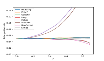
(a)

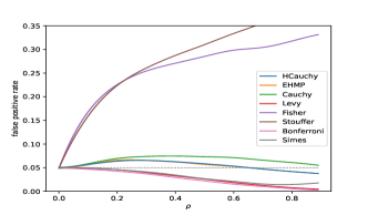
(b)

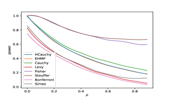
(c)

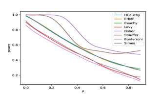
(d)

Figure 4: Comparison of combination tests in false positive rate and power.

We compare the empirical performance of combination tests by checking the false positive rate (Type I error) and power ($1-$ Type II error) in the presence of dependence between studies. The combination tests we consider include the Fisher’s combination test, Stouffer’s Z-score test, Bonferroni correction, Simes’ test [Simes 1986], Lévy combination test [Wilson 2021], CCT [Liu and Xie 2020], and our proposed HCCT and EHMP.

First, we generate the vector of individual test statistics $\boldsymbol{X}$ from $\mathcal{N}_{m}(\boldsymbol{\theta},\boldsymbol{\Sigma})$ with $\boldsymbol{\theta}=\boldsymbol{0}$ under the null, where $m$ is the number of studies. We consider $m=20,100,500$ for each of the following correlation matrix $\boldsymbol{\Sigma}=(\sigma_{ij})$:

• AR-$1$ correlation: $\sigma_{ij}=\rho^{\lvert i-j\rvert}$ for $1\leq i,j\leq m$, where $\rho\in[0,1)$;

• Equi-correlation: $\sigma_{ij}=\rho$ for $1\leq i,j\leq m$, where $\rho\in[0,1)$.

The results for $m=500$ are shown in Figures˜4(a) and 4(b) respectively.

Second, we investigate how signal strength and sparsity could influence the power of different tests along with levels of dependence. We consider the vector of individual test statistics $\boldsymbol{X}$ generated from the alternative $\mathcal{N}_{m}(\boldsymbol{\mu},\boldsymbol{\Sigma})$, where $\boldsymbol{\mu}=(\mu_{i})$ and $\boldsymbol{\Sigma}=(\sigma_{ij})$. Following the simulation setup of Liu and Xie [2020] and Wilson [2021], we fix $\boldsymbol{\Sigma}$ to be the equi-correlation matrix as defined above and set

$$\small\normalsize\mu_{i}=\begin{cases}\sqrt{2r\log m_{0}}&1\leq i\leq m_{0}=\lfloor m^{1-s}\rfloor\\ 0&m_{0}+1\leq i\leq m\end{cases},\small\normalsize$$

where $s\in[0,1)$ and $r>0$ are hyperparameters controlling the strength and sparsity. Figure˜4(c) shows results for $s=0$ and $r=0.1$ (weak signal) and Figure˜4(d) shows results for $s=r=0.3$ (sparse signal).

We observe that Fisher’s test and Stouffer’s test suffer from high false positive rates for dependent studies. Similar issues have been observed in Ling and Rho [2022] for their stable combination test (SCT) with $\alpha>1$. These methods share a common feature: their corresponding $\nu$ is attracted to stable distributions $S(\alpha,\beta,c,\mu)$ with $\alpha>1$. On the other hand, we see that LCT [Wilson 2021], Bonferroni correction, and Simes’ test result in overly conservative tests with low powers for dependent studies. Here the score of LCT is defined as (2.1) using the Lévy distribution $S(1/2,1,1,0)$. As a generalization of LCT, Ling and Rho [2022] observed similar phenomena with $\nu\sim S(\alpha,1,1,0)$ and $\alpha<1$. Moreover, the Bonferroni correction uses the minimum $p$-values, which could be regarded as the limit of (2.1) with $\nu\sim\text{Pareto}(\alpha,1)$ and $\alpha\to 0$ [Fang et al. 2023]. Note that Pareto$(\alpha,1)$ is attracted to $S(\alpha,1,c,\mu)$ for some $c$ and $\mu$. Finally, Simes’ test is a modification of the Bonferroni approach by accounting for ordered $p$-values. In general, we observe that with $\nu$ attracted to stable distributions $S(\alpha,\beta,c,\mu)$ where $\alpha<1$, the combination tests given by (2.1) show lower power but better validity.

Finally, CCT [Liu and Xie 2020], HCCT and EHMP strike a good balance between validity and power. Notably their test scores are given by (2.1) with $\nu$ being Cauchy, Half-Cauchy and Pareto$(1,1)$ respectively. These three distributions are in the domain of attraction of the Landau family, i.e., $S(\alpha,\beta,c,\mu)$ with $\alpha=1$. For simplicity we have only presented the results for $p$-values obtained from multivariate normal with different correlations. However, we also conduct simulations for other dependency structures including multivariate t, Farlie–Gumbel–Morgenstern (FGM) copula and Ali–Mikhail–Haq (AMH) copula, the results of which are shown in Appendix˜B, where we also demonstrate the sensitivity to large $p$-value when $v$ is not attracted to $S(\alpha,\beta,c,\mu)$ with $\alpha=1$.

3 Confidence Regions from Inverting Half-Cauchy Combination Tests

3.1 Univariate Cases

Suppose there are $m$ possibly dependent studies, the $j$-th of which provides $\widehat{\theta}_{j}$ as its estimator of the common estimand $\theta\in\mathbb{R}$, together with a variance estimator $\widehat{\sigma}_{j}^{2}$. For many common studies, it is acceptable to approximate the distribution of $(\widehat{\theta}_{j}-\theta)/\widehat{\sigma}_{j}$ by the $t$-distribution with $k_{j}$ degrees of freedom. That is, we can compute the (two-sided) $p$-value as

$$\small\normalsize\textstyle p_{j}=2\Bigl{\{}1-F^{(j)}\Bigl{(}\widehat{\sigma}_{j}^{-1}\lvert\widehat{\theta}_{j}-\theta\rvert\,\Bigr{)}\Bigr{\}},\small\normalsize$$ (3.1)

where $F^{(j)}$ is the CDF of the $t$ distribution with $k_{j}$ degrees of freedom, which includes $\mathcal{N}(0,1)$ when we permit $k_{j}=\infty$.

A $(1-p)$-level confidence interval for $\theta$ can then be constructed based on the generalized combination test from (2.1):

$$\small\normalsize\sum_{j=1}^{m}w_{j}F_{\nu}^{-1}\Bigl{\{}2F^{(j)}\Bigl{(}\widehat{\sigma}_{j}^{-1}\lvert\widehat{\theta}_{j}-\theta\rvert\,\Bigr{)}-1\Bigr{\}}\leq F_{\nu,\boldsymbol{w}}^{-1}(1-p).\small\normalsize$$ (3.2)

Here $F_{\nu}$ denotes the CDF of $\nu$, and $F_{\nu,\boldsymbol{w}}$ represents the CDF of $T_{\nu,\boldsymbol{w}}$ for independent studies, as defined in (2.1). In the case of HCCT, $\nu$ is the standard Half-Cauchy, and hence we will write $F_{\textup{HC}}$ for $F_{\nu}$. The following is our main algebraic result. Notably the validity of the theorem itself is guaranteed for any actual dataset, not depending on whether (3.1) provides a valid $p$-value or not, (e.g., whether it is uniformly distributed under the null). Nevertheless, the validity of the $p$-value defined through (3.1) is important in obtaining the correct coverage.

Theorem 3.1.

For HCCT, the solution set of (3.2) is always a single (but possibly empty) finite interval.

As a side note, we can establish similar connectivity results for the EHMP. However, connectivity cannot be guaranteed for most other combination tests with general $\nu$. We provide some intuition here; see Appendix˜D for formal results.

(a)

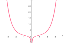
(b)

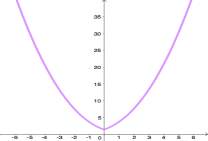
(c)

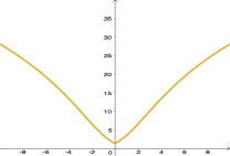
(d)

Figure 5: Plots of $g_{j}(\theta)=F_{\nu}^{-1}\bigl{\{}2F^{(j)}(\lvert\theta\rvert)-1\bigr{\}}$, where the first distribution in the caption refers to $F_{v}$, and the second to $F^{(j)}$.

To illustrate, if we would like the left-hand side of (3.2) to be connected for arbitrary $w_{j}$, $\widehat{\theta}_{j}$ and $\widehat{\sigma}_{j}$’s, the function

$$g_{j}(\theta)=F_{\nu}^{-1}\Bigl{\{}2F^{(j)}\Bigl{(}\widehat{\sigma}_{j}^{-1}\lvert\widehat{\theta}_{j}-\theta\rvert\Bigr{)}-1\Bigr{\}}$$

must be convex (see Lemma˜D.1). To ensure the convexity of $g_{j}$, two necessary conditions must be satisfied, the essence of which is again captured by the term “heavily right”. First, the density $f_{\nu}$ must be monotone decreasing on its support, as shown in Lemma˜D.2 of Appendix˜D, since otherwise $g_{j}(\theta)$ is non-convex near $\theta=0$. Notably, this condition excludes all $\alpha$-stable distributions for $\nu$. For example, as shown in Figures˜5(a) and 5(b), the function $g_{j}$ is convex when $\nu$ follows a HC distribution, whereas it is non-convex for $\nu$ following a Cauchy distribution.

Second, as established by Lemma˜D.2, the convexity of $g_{j}(\theta)$ (as $\lvert\theta\rvert\to\infty$) implies that the right tail of the density for $F_{\nu}$ cannot be lighter than of the $F^{(j)}$. To ensure this property for any choice of $F^{(j)}$ in the $t_{d}$ family with integer degrees of freedom $d$, HC is near-optimal, because it is the same as $t_{1}$. As an illustration of this requirement, consider the Fisher’s combining rule, which sets $\nu=\chi^{2}_{2}$. When $\sigma_{j}$ is known, we can take $F^{(j)}$ as ${\mathcal{N}}(0,1)$, hence $\nu=\chi^{2}_{2}$ is acceptable because its right tail is heavier than that of normal. Indeed, Figure˜5(c) shows the resulting $g_{j}(\theta)$ is convex, yielding a single confidence interval for $\theta$ regardless of its confidence level. In contrast, when $\sigma_{j}$ is unknown and hence we must choose $F^{(j)}$ from the $t_{d}$ family with $d<\infty$, say, $t_{10}$, then the density of $F^{(j)}$ will have heavier tail than that of $v=\chi^{2}_{2}$. This will necessarily destroy the convexity of $g_{j}(\theta)$, as seen in Figure˜5(d), leading to disconnected confidence sets. (For this reason, we assign a neutral rating to Fisher’s test regarding its performance on confidence regions, as displayed in Table˜1.)

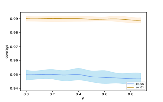
(a)

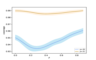
(b)

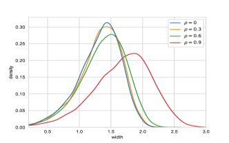
(c)

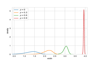
(d)

Figure 6: Confidence intervals from $1$-dimensional HCCT.

To numerically compute the confidence intervals, we apply Brent’s method [Brent 1971]—the default optimization and root-finding algorithm for scalar functions in the Python package SciPy—to find both the minimizer of the score and the root of (3.2). We then consider the same simulation settings as in Section˜2.5 to obtain confidence intervals for $\theta$ using the approach discussed above. Figure˜6 presents the actual coverage and widths of the confidence intervals under two different correlation structures. We observe that, in general, the coverage for dependent studies is nearly as good as in the independent case. However, when the estimators are equally correlated with $\rho$ around $0.25$, the coverage slightly falls below the desired level. Additionally, HCCT demonstrates better robustness when conducted at a $0.01$ significance level.

We also observe that the widths of the confidence intervals increase as $\rho$ grows. This effect is especially pronounced in the equi-correlation setup, demonstrating that our approach is robust to the underlying dependence structure by being adaptive to it. Intuitively, fixing the variance of each individual estimator, higher correlations between studies mean fewer effective number of (independent) studies, and hence larger uncertainties and wider confidence intervals.

3.2 Multivariate Cases

Next, we consider combining $m$ studies to obtain a set estimate for $\boldsymbol{\theta}\in\mathbb{R}^{d}$, where $d$ can be arbitrarily large. Suppose we have an estimator $\widehat{\boldsymbol{\xi}}_{j}\in\mathbb{R}^{d_{j}}$ from the $j$-th study for $P_{j}\theta$, where $\boldsymbol{P}_{j}\in\mathbb{R}^{d_{j}\times d}$ is a full-rank matrix with $d_{j}\leq d$. We also assume that the $j$-th study provides a positive definite covariance estimator $\widehat{\boldsymbol{\Sigma}}_{j}$ for $\widehat{\boldsymbol{\xi}}_{j}$. Note that $P_{j}$ or $d_{j}$ can vary with $j$, and that $d_{j}<d$, is critical for dealing with arbitrary dimension $d$, since the choices of $d_{j}$’s and $\boldsymbol{P}_{j}$’s allow us to form different lower dimensional projections, and to ensure $\widehat{\boldsymbol{\Sigma}}_{j}>0$. For example, we can always choose $d_{j}=1$ for all $j$’s.

As a natural generalization from the $t$ approximation in the univariate case, here we adopt the Hotelling’s $T^{2}$ distribution by assuming that it is acceptable to postulate that, given the value of $\theta$

$$\small\normalsize(\widehat{\boldsymbol{\xi}}_{j}-\boldsymbol{P}_{j}\boldsymbol{\theta})^{\top}\widehat{\boldsymbol{\Sigma}}_{j}^{-1}(\widehat{\boldsymbol{\xi}}_{j}-\boldsymbol{P}_{j}\boldsymbol{\theta})\sim\ T^{2}(d_{j},k_{j})=\frac{d_{j}k_{j}}{k_{j}+1-d_{j}}F(d_{j},k_{j}+1-d_{j}),\small\normalsize$$ (3.3)

where $T^{2}(d_{j},k_{j})$ is the Hotelling’s $T^{2}$-distribution, related to the $F$-distribution as indicated, and the degrees of freedom with $\widehat{\boldsymbol{\Sigma}}_{j}$, $k_{j}$ are supplied by the $j$-th study. Consequently, the $p$-value for testing $\theta$ from the $j$-th study is given by

$$\small\normalsize p_{j}=1-F^{(j)}\bigl{\{}(\widehat{\boldsymbol{\xi}}_{j}-\boldsymbol{P}_{j}\boldsymbol{\theta})^{\top}\widehat{\boldsymbol{\Sigma}}_{j}^{-1}(\widehat{\boldsymbol{\xi}}_{j}-\boldsymbol{P}_{j}\boldsymbol{\theta})\bigr{\}},\small\normalsize$$ (3.4)

where $F^{(j)}$ is the CDF of $T^{2}(d_{j},k_{j})$ when $k_{j}<\infty$ or of $\chi^{2}$ with $d_{j}$ degrees of freedom when $k_{j}=\infty$, which is applicable when $\widehat{\Sigma}_{j}$ is considered to be known or deterministic. The $(1-p)$-level confidence region for $\boldsymbol{\theta}$ is then obtained by inverting the HCCT, resulting in the following inequality:

$$\sum_{j=1}^{m}w_{j}F_{\textup{HC}}^{-1}\left[F^{(j)}\bigl{\{}(\widehat{\boldsymbol{\xi}}_{j}-\boldsymbol{P}_{j}\boldsymbol{\theta})^{\top}\widetilde{\boldsymbol{\Sigma}}_{j}^{-1}(\widehat{\boldsymbol{\xi}}_{j}-\boldsymbol{P}_{j}\boldsymbol{\theta})\bigr{\}}\right]\leq F_{\textup{HC},\boldsymbol{w}}^{-1}(1-p).$$ (3.5)

The following result generalizes Theorem˜3.1, but again not relying on the validity of the distributional assumption (3.3).

Theorem 3.2.

For HCCT, the solution set of (3.5) is a convex region (which can be empty) if $k_{j}\geq d_{j}+1$ ($1\leq d_{j}\leq d$) for all $j=1,\dots,m$. Furthermore, the confidence region is bounded if $\{\operatorname{Row}(\boldsymbol{P}_{j}),j\in J_{+}\}$ span $\mathbb{R}^{d}$, where $J_{+}=\{j:w_{j}>0\}$.

Numerically, we can use (3.5) to check whether a given point lies within the confidence region. A point estimator can be obtained by minimizing the convex function on the left-hand side of (3.5), and hence it is always inside the confidence region, as long as the region is not empty. For this optimization, we can apply Powell’s method [Powell 1964] or the L-BFGS algorithm [Fletcher 1987]. In the two-dimensional case, we can explicitly plot the confidence regions by first finding the point estimator and then using grid search to obtain the full boundary of the region. For higher dimensions ($d\geq 3$), we provide functions to compute any one-dimensional slices and to plot two-dimensional slices of the $d$-dimensional confidence region, which are confidence regions conditioning on the values of $\theta$ in the given slice.

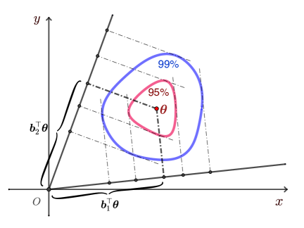
Figure 7: Illustration of obtaining simultaneous confidence intervals from confidence regions via projection. The plot shows $95\%$ and $99\%$ simultaneous confidence intervals for $\boldsymbol{b}_{i}^{\top}\boldsymbol{\theta}$ ($i=1,2$ with $\lVert\boldsymbol{b}_{i}\rVert_{2}=1$).

Another way to utilize multi-dimensional confidence regions is to obtain simultaneous confidence intervals for $\boldsymbol{b}^{\top}\boldsymbol{\theta}$, given any $\boldsymbol{b}\in\mathbb{R}^{d}$, by minimizing and maximizing $\boldsymbol{b}^{\top}\boldsymbol{\theta}$ subject to (3.5). A simultaneous confidence interval is one that provides joint coverage across multiple linear combinations of $\boldsymbol{\theta}$. This means that the interval holds with a specified confidence level for all the directions $\boldsymbol{b}$ considered. As illustrated in Figure˜7, confidence regions naturally induce simultaneous confidence intervals by projecting onto specific directions. Notably when confidence regions are not accessible, it is common to use the Bonferroni correction to obtain simultaneous confidence intervals from non-simultaneous ones, which tends to be significantly more conservative in practice.

These problems are convex optimizations with a linear objective and a nonlinear constraint, making penalty or barrier (interior-point) methods particularly suitable [Boyd and Vandenberghe 2004]. In this context, we implement a penalty method by solving the following unconstrained convex problems with a sufficiently large $\lambda$ value (we set $\lambda=\exp{20}$ by default) using Powell’s method or the L-BFGS algorithm mentioned earlier:

$$\small\normalsize\textstyle\operatorname{minimize}_{\boldsymbol{\theta}}\ \boldsymbol{b}^{\top}\boldsymbol{\theta}+\lambda\Bigl{[}\sum_{j=1}^{m}w_{j}F_{\nu}^{-1}\mathbin{\vbox{\hbox{\scalebox{0.6}{$\circ$}}}}F_{j}\bigl{\{}(\widehat{\boldsymbol{\xi}}_{j}-\boldsymbol{P}_{j}\boldsymbol{\theta})^{\top}\widetilde{\boldsymbol{\Sigma}}_{j}^{-1}(\widehat{\boldsymbol{\xi}}_{j}-\boldsymbol{P}_{j}\boldsymbol{\theta})\bigr{\}}-F_{\nu,\boldsymbol{w}}^{-1}(1-p)\Bigr{]}\vee 0,$$

$$\textstyle\operatorname{maximize}_{\boldsymbol{\theta}}\ \boldsymbol{b}^{\top}\boldsymbol{\theta}-\lambda\Bigl{[}\sum_{j=1}^{m}w_{j}F_{\nu}^{-1}\mathbin{\vbox{\hbox{\scalebox{0.6}{$\circ$}}}}F_{j}\bigl{\{}(\widehat{\boldsymbol{\xi}}_{j}-\boldsymbol{P}_{j}\boldsymbol{\theta})^{\top}\widetilde{\boldsymbol{\Sigma}}_{j}^{-1}(\widehat{\boldsymbol{\xi}}_{j}-\boldsymbol{P}_{j}\boldsymbol{\theta})\bigr{\}}-F_{\nu,\boldsymbol{w}}^{-1}(1-p)\Bigr{]}\vee 0.$$

As a proof-of-concept demonstration, we simulate $m$ dependent studies for estimating $\boldsymbol{\theta}$. Let $\widehat{\boldsymbol{\theta}}^{(j)}=\bigl{\{}\widehat{\theta}_{1}^{(j)},\dots,\widehat{\theta}_{d}^{(j)}\bigr{\}}^{\top}$ ($j=1,\dots,m$) represent the estimator from the $j$-th study. For simplicity, we set $\boldsymbol{\theta}=\boldsymbol{0}$ and generate:

$$\small\normalsize\textstyle\Bigl{\{}\widehat{\theta}_{1}^{(1)},\dots,\widehat{\theta}_{1}^{(m)},\dots\dots,\widehat{\theta}_{d}^{(1)},\dots,\widehat{\theta}_{d}^{(m)}\Bigr{\}}^{\top}\sim\mathcal{N}\Bigl{\{}\boldsymbol{0},\operatorname{diag}\bigl{(}\boldsymbol{M}_{\rho},\dots,\boldsymbol{M}_{\rho}\bigr{)}\Bigr{\}},\small\normalsize$$

where $\boldsymbol{M}_{\rho}=(1-\rho)\boldsymbol{I}_{m}+\rho\mathbf{1}\mathbf{1}^{\top}$. Hence the between-study correlation is $\rho$, while the within-study correlation is zero.

We then apply HCCT approach with $P_{j}=I_{d},j=1,\dots,m$. Figure˜8 shows a single run with $m=500$, $d=2$, and $\rho=0,0.3,0.6,0.9$, respectively. We observe that the confidence regions become larger as the correlation level increases, even though our approach does not directly incorporate correlations in the input or as part of the estimation process. This again suggests that the method is robust to the correlation structure by adapting to it. For instance, when $\rho=0.9$, the individual estimates are often concentrated away from the true value. In Figure˜8(d), most estimates cluster around $(2.2,-0.1)$, while the true value of $\boldsymbol{\theta}$ is $(0,0)$. As a result, a larger confidence region is necessary to maintain 95% coverage. This observation is consistent with the experimental results for $d=1$ shown in Figure˜6(d).

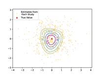
(a)

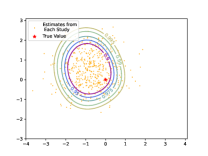
(b)

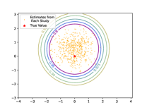
(c)

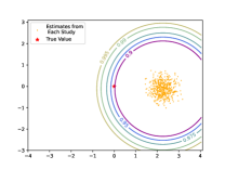
(d)

Figure 8: Contour plots of confidence regions from $2$-dimensional HCCT.

We further examine the coverage of our constructed confidence regions in Figure˜9 with varying numbers of studies ($m=10,500$) and dimensions ($d=2,5,10,25$) across different levels of dependence $\rho=0,0.1,\dots,0.9$. Specifically, the experimental results here are obtained from $1000$ different runs for each $\rho$, $m$ and $d$. In general, the behavior for $d>1$ is not significantly different from the univariate case (see Figure˜6(b)). All regions have essentially the nominal coverage at the $99\%$ level, though at the $95\%$ level, there are some small deterioration of coverage when $m$ is large. The fact that our HCCT approach performs better at the 99% level is consistent with our expectation from the nature of tail approximation. The $U$-shape behavior in the amount of deterioration, as most visible the $95\%$ level and with $m=500$, is also consistent with the fact the Half-Cauchy approach is strictly valid when $\rho=0$ or $\rho=1$. Currently, however, we have no theoretical results on bounding the largest approximation error or the amount of dependence when it occurs.

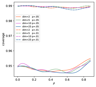
(a)

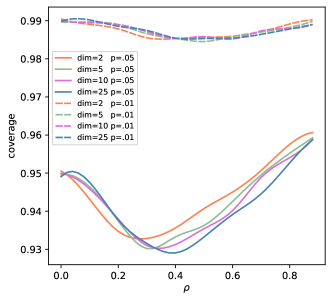
(b)

Figure 9: Coverage of $d$-dimension confidence regions from HCCT.

3.3 Understanding and Dealing with Empty Confidence Sets

An important consideration is that the solution set of (3.2) or of (3.5) can be empty when $\nu$ is HC and $m>1$, a phenomenon that cannot occur when $\nu$ is Cauchy. To see this clearly, compare $T_{\textup{CCT}}$ of (2.2) with $T_{\textup{HCCT}}$ of (2.3), where $p_{j}$ is given by (3.1), by explicating all three terms as functions of $\theta$, that is

$$T_{\textup{CCT}}(\theta)=\sum_{j=1}^{m}w_{j}\cot(\pi p_{j}(\theta)),\quad T_{\textup{HCCT}}(\theta)=\sum_{j=1}^{m}w_{j}\cot\left\{\frac{\pi}{2}p_{j}(\theta)\right\},\quad p_{j}(\theta)=2\left\{1-F^{(j)}\left(\frac{\lvert\widehat{\theta}_{j}-\theta\rvert}{\widehat{\sigma}_{j}}\right)\right\},$$ (3.6)

where $F^{(j)}$ is the CDF of a $t$ or normal distribution. Consequently, $p_{j}(\widehat{\theta}_{j})=1$ for any $j$, which means $T_{\textup{CCT}}(\theta_{j})=-\infty$ because $\lim_{x\uparrow\pi}\cot(x)=-\infty$. Hence any confidence region in the form of $C_{K}(\theta)=\{\theta:T_{\textup{CCT}}(\theta)\leq K\}$ must contain all $\widehat{\theta}_{j}$’s, regardless of the value of cut-off $K$, as long as it is finite; we have seen two such examples in Figure˜1.

In contrast, because $\cot\left(\frac{\pi}{2}p_{j}(\theta)\right)\geq 0$ for all $\theta$, we see that $T_{\textup{HCCT}}(\theta)\geq 0$, and indeed it is possible for $\min_{\theta}T_{\textup{HCCT}}(\theta)=T_{\min}>K$, in which case, the set $C_{K}^{+}(\theta)=\{\theta:T_{\textup{HCCT}}(\theta)\leq K\}$ will be empty. In particular, because $F^{(j)}(x)\leq F_{\textup{Cauchy}}(x)=\pi^{-1}\arctan(x)+0.5$ when $x\geq 0$, we have the following lower bound

$$T_{\textup{HCCT}}(\theta)\geq\sum_{j=1}^{m}w_{j}\cot\biggl{\{}\frac{\pi}{2}-\arctan\Bigl{(}\frac{\lvert\widehat{\theta}_{j}-\theta\rvert}{\widehat{\sigma}_{j}}\Bigr{)}\biggr{\}}=\sum_{j=1}^{m}\frac{w_{j}}{\widehat{\sigma}_{j}}\lvert\widehat{\theta}_{j}-\theta\rvert\geq\sum_{j=1}^{m}\frac{w_{j}}{\widehat{\sigma}_{j}}\lvert\widehat{\theta}_{j}-\widehat{\theta}_{\textup{med}}\rvert,$$ (3.7)

where $\widehat{\theta}_{\textup{med}}$ is the median of the discrete distribution on $\{\widehat{\theta}_{j},j=1,\ldots,m\}$ with $\mathbb{P}(\widehat{\theta}=\widehat{\theta}_{j})\propto w_{j}/\widehat{\sigma}_{j}$.

The inequality (3.7) is telling, since the lower bound is a measure of inconsistency among the $m$ studies, taking into account the weights. Indeed, $T_{\min}$ is the smallest possible weighted $t$-test statistics against a common null from the $m$ studies, that is, by fitting the null to the minimizer $\theta=\theta^{\ast}$. If this fitted null still can be rejected at the level $p$, then what is being rejected is not really the null value, but rather the existence of a common value across the $m$ studies. The increased probability for the occurrence of an empty set with the increased significance level $p$ can be understood intuitively from John Tukey’s notion of “outerval", the complement to the confidence interval. That is, constructing a confidence interval of $\theta$ for further considerations should be described as “constructing outerval to eliminate implausible values as declared by our chosen criterion”, as discussed in Meng [2022]. The larger the significance level $p$, the less stringent the criterion for implausibility, and hence higher chance to declare that nothing is acceptable.

While an empty set is reasonable for ensuring declared confidence coverage in repeated experiments, it is problematic in real-data analyses. To address this, we leverage the flexibility of HCCT in assigning weights to different studies and propose a general adaptive procedure. Specifically, we can mitigate the problem by identifying studies that contribute most to the inconsistency and appropriately adjusting their weights in the combination test, potentially reducing some to zero. For example, we can set $w_{j}=0$ if the largest change in the low bound in (3.7) occurs when we drop the $j$-th study, and continue such a process until a non-empty confidence set is obtained. Intuitively, searching for a non-empty solution can only increase the (conditional) confidence coverage. This intuition is formalized in the following result.

Proposition 3.3.

Consider $\mathcal{W}=\{\boldsymbol{w}=(w_{1},\cdots,w_{m})^{\top}:w_{j}\geq 0\text{ for }1\leq j\leq m,\ w_{1}+\cdots+w_{m}=1\}$ as the class of weight vectors. For any $\boldsymbol{w}\in\mathcal{W}$, let $z_{\boldsymbol{w}}$ be a weight-dependent threshold such that $\mathbb{P}\bigl{(}T_{\textup{HCCT},\boldsymbol{w}}\leq z_{\boldsymbol{w}}\bigr{)}\geq 1-p,$ where $T_{\textup{HCCT}}(\boldsymbol{w})$, defined by the left-hand-side of (3.2) or (3.5), also depends on the weight vector $\boldsymbol{w}$. Let $\tau$ be any stopping time for the random sequence: $T_{\textup{HCCT},\boldsymbol{w}^{(0)}},T_{\textup{HCCT},\boldsymbol{w}^{(1)}},T_{\textup{HCCT},\boldsymbol{w}^{(2)}},\ldots,$ where $\boldsymbol{w}^{(k)}$ can be chosen adaptively based on the previous sequence and any data or statistic for individual studies for $k\geq 1$. Then the following procedure produces a confidence region with at least $(1-p)$ coverage:

• Start with an arbitrary $\boldsymbol{w}^{(0)}\in\mathcal{W}$ and obtain the solution set $R^{(0)}$ of $T_{\textup{HCCT},\boldsymbol{w}^{(0)}}\leq z_{\boldsymbol{w}^{(0)}}$.

• For $1\leq k\leq\tau$, we choose $\boldsymbol{w}^{(k)}\in\mathcal{W}$ and get the solution set $R^{(k)}$ of $T_{\textup{HCCT},\boldsymbol{w}^{(k)}}\leq z_{\boldsymbol{w}^{(k)}}$.

• Report $R^{\ast}=\bigcup_{k=0}^{\tau}R^{(k)}$.

As an immediate application of Proposition˜3.3, we can set $\tau$ as the stopping time when we find the first non-empty solution. Then by construction, $R^{(k)}=\emptyset$ for all $k<\tau$, implying $R^{(\tau)}=R^{\ast}$. Therefore, $R^{(\tau)}$, as an adaptive confidence-region generating procedure, will have at least $1-p$ coverage. Intuitively, an empty solution set represents an extreme case where conditional coverage is zero, and the procedure addresses this by enhancing conditional coverage.

From a hypothesis testing perspective, one might be concerned with the practice of keeping search for a significant level until we find it acceptable. Whereas it is critical to be always vigilant about $p$-hacking and similar abuses, the issue of empty set is an issue of being overly significant because the null is rejected for its inconsistencies with the data (at the declared level) in aspects that are not the primary target of the testing. To attach a significance level that is consistent with testing the primary aspects of the null, we can then search for the significance level in the first instance where testing the primary aspects of the null is no longer overshadowed by the inconsistency with the secondary aspects of the hull. This empty-set issue also reminds us that even if we have no interest in inverting a test, we should consider the properties of the rejection regions and mindfully look for anomalies that are otherwise masked by the direct testing results.

4 A Divide-and-Combine Strategy for High-Dimensional Mean Estimation

4.1 Leveraging Hotelling’s $T^{2}$ but Circumventing Its Curse of Dimension

Many applications in practice involve hypothesis tests and point or set estimators for the mean vector $\boldsymbol{\theta}$ from multivariate normal samples with an unknown covariance matrix $\boldsymbol{\Sigma}$. A classical approach to this problem is Hotelling’s $T^{2}$-test, which provides an ellipsoidal confidence region for $\boldsymbol{\theta}$. However, Hotelling’s test requires estimation of the full covariance (or precision) matrix, which poses significant numerical and statistical challenges in high dimensions [Bai and Saranadasa 1996; Pan and Zhou 2011].

A considerable body of literature has focused on advancing techniques for covariance matrix estimation in high dimensions [Bickel and Levina 2008; Cai and Yuan 2012; Cai et al. 2016; Avella-Medina et al. 2018; Lam 2020; Liu and Ren 2020; Goes et al. 2020]. Various approaches have been proposed to address these challenges, including the use of diagonal matrices [Wu et al. 2006; Srivastava and Du 2008; Tony Cai et al. 2014; Dong et al. 2016], block-diagonal matrices [Feng et al. 2017], U-statistics [He et al. 2021; Li 2023], random projections [Lopes et al. 2011; Srivastava et al. 2016], and regularization procedures [Chen et al. 2011; Li et al. 2020].

Our HCCT provides a divide-and-combine strategy that circumvents the need for estimating the full covariance matrix. A key advantage of our method is that the resulting confidence regions are guaranteed to be convex and bounded, even when the sample size is smaller than the dimension $d$, which contrasts with Hotelling’s test that requires a sample size larger than $d$. Moreover, our approach can potentially yield smaller confidence regions compared to Hotelling’s test, offering further practical benefits.

Our method leverages the same set of samples to construct $m$ virtual sub-studies, where we estimate $\boldsymbol{P}_{j}\boldsymbol{\theta}$ for $j=1,\dots,m$ using linear transformations of the original data. The matrices $\boldsymbol{P}_{j}$ are $d_{j}\times d$ matrices, where $d_{j}$ can be much smaller than $d$. The estimator in each sub-study is then derived using the Student’s $t$-test (for $d_{j}=1$) or Hotelling’s $T^{2}$-test (for $d_{j}\geq 2$). These estimators are generally dependent, but our HCCT method allows us to combine the resulting $p$-values, and invert the combination test to generate confidence regions for $\boldsymbol{\theta}$, without much concern about their dependence.

As shown in Theorem˜3.2, the resulting confidence region is guaranteed to be convex and bounded, as long as the row vectors of $\{\boldsymbol{P}_{1},\boldsymbol{P}_{2},\dots,\boldsymbol{P}_{m}\}$ span $\mathbb{R}^{d}$ and the sample size (i.e., $1+$ the degrees of freedom for one-sample tests) is not smaller than $\max\{d_{j}+2\}$. Notably, this sample size can be much smaller than $d$. In particular, because we can choose $d_{j}=1$ for all $j$’s—in which case we will need $m\geq d$ to ensure boundedness—the minimum sample size required for our method is 3, regardless of $d$. In contrast the traditional $d$-dimensional Hotelling’s test—which corresponds to choosing $m=1$ and $P_{1}=I_{d}$ using our notation—requires at least $d+1$ samples.

Because our approach only requires the estimation of covariance matrices within the low-dimensional sub-studies, it is more scalable and computationally efficient in high-dimensional settings. Specifically, if we choose the $\boldsymbol{P}_{j}$’s as projections into subspaces spanned by subsets of the coordinates of $\mathbb{R}^{d}$, we only need to estimate certain block-diagonal entries of $\boldsymbol{\Sigma}$. Importantly, the dependence structure among the remaining entries of $\boldsymbol{\Sigma}$ is automatically accounted for by the robustness properties of HCCT, enabling us to handle more complex covariance structures without needing to estimate the full matrix.

Since HCCT is robust to arbitrary correlations between different sub-studies, any choice of $\boldsymbol{P}_{j}$’s can still provide reasonably accurate coverage. In particular, beyond simple coordinate projections, $\boldsymbol{P}_{j}$’s can also be derived from random projections or directions informed by a principal component analysis of the data. As demonstrated in Proposition˜2.6, redundancy in the tests does not negatively impact the results, allowing the number of virtual sub-tests $m$ to potentially exceed the dimension $d$. Moreover, the method remains effective even if the underlying distribution $\mathcal{N}(\boldsymbol{\theta},\boldsymbol{\Sigma})$ is degenerate with a low-rank $\boldsymbol{\Sigma}$, provided that the sub-study covariance matrices $\boldsymbol{\Sigma}_{j}$ are full rank. This highlights the versatility and robustness of our approach across a wide range of settings.

However, despite the flexibility of our approach, it is desirable to choose $\boldsymbol{P}_{j}$’s that lead to more compact confidence regions, while maintaining the scalability and computational efficiency. Much research is needed to understand the impact of the choices of $m$ and $\{\boldsymbol{P}_{j},j=1,\ldots,m\}$ on the statistical and computational efficiencies of our method. We invite all interested to study and explore with us the full potential of this new approach, and to seek optimal compromise.

It is worthwhile to broadly investigate the divide-and-combine strategy because it enhances our toolkit for the popular divide-and-conquer strategies. Generally speaking, there have been two broad classes of divide-and-conquer methods. One class divides a big dataset into many independent smaller ones, performs analysis on each subset for the whole problem, and then combines the individual results via rules based on independence assumptions [Chen et al. 2021]. The other class divides the problem itself into sub-problems, such as breaking down high dimensions [Sabnis et al. 2016; Gao and Tsay 2023]. Our divide-and-combine strategy belongs to the second class, as it breakdown the estimation problem into many sub-problems via projections, and use all the data for each sub-problem. These modularized solutions likely have complex dependence among them since they are all derived from the same data. This is where HCCT or other dependence resilient combination rules become handy and powerful, making the divide-and-combine strategy practically viable. The fact that all data are used for each sub-problem also means that we have better chance to retain statistical efficiency.

4.2 Simulation Study with Normal Samples

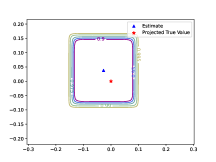
(a)

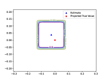
(b)

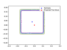
(c)

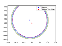
(d)

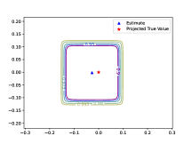
(e)

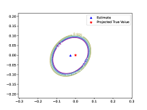
(f)

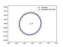
(g)

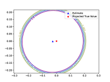
(h)

Figure 10: 2d slices of confidence regions passing through the point estimate with varying $d_{0}$ in the multivariate normal study.

For our first simulation study, we generate $n$ i.i.d. samples $\boldsymbol{X}_{1},\dots,\boldsymbol{X}_{n}\in\mathbb{R}^{d}$ from the ideal distribution $\mathcal{N}(\boldsymbol{\theta},\boldsymbol{M}_{\rho})$, where $\boldsymbol{\theta}=\boldsymbol{0}$ and $\boldsymbol{M}_{\rho}=(1-\rho)\boldsymbol{I}_{d}+\rho\mathbf{1}\mathbf{1}^{\top}$. We assume no prior information about $\boldsymbol{\theta}$ or $\boldsymbol{M}_{\rho}$ beyond the samples themselves. The goal is to construct a confidence region for $\boldsymbol{\theta}$.

To achieve this, we apply HCCT with $\boldsymbol{P}_{j}$ being coordinate projections. Specifically, we fix $1\leq d_{0}<d$, and split the $d$-dimensional study evenly into multiple sub-studies. Letting $\boldsymbol{X}_{i}=(X_{i1},\dots,X_{id})^{\top}$ and $d=md_{0}+r$, where $0\leq r\leq m-1$, we observe $\boldsymbol{P}_{j}\boldsymbol{X}_{i}=(X_{i,k_{j-1}+1},\dots,X_{i,k_{j}})^{\top}$ with $k_{j}=d_{0}j+\min\{j,r\}$ for $i=1,\dots,n$ and $j=1,\dots,m$, which are i.i.d. from $\mathcal{N}\Bigl{(}\boldsymbol{P}_{j}\boldsymbol{\theta},\boldsymbol{P}_{j}\boldsymbol{M}_{\rho}\boldsymbol{P}_{j}^{\top}\Bigr{)}$ in the $j$-th sub-study for $j=1,\dots,m=\lfloor d/d_{0}\rfloor$. We then conduct Hotelling’s $T^{2}$-test for $\boldsymbol{P}_{j}\boldsymbol{\theta}$ in each sub-study, and combine the results via HCCT.

For simplicity, we fix $\rho=0.6$, $d=100$, $n=1000$, and $d_{0}=1,5,25,100$. We repeat the experiments $2000$ times with a significance level of $0.05$ and find that the coverage of the confidence regions is $0.944$, $0.953$, $0.945$, and $0.956$, respectively, confirming empirically the validity of our method regardless of the choice of $d_{0}$ in this ideal case.

Figure˜10 shows the intersection of an obtained confidence region with a plane passing through the same point estimate, using the same set of samples. In particular, $d_{0}=100$ corresponds to Hotelling’s $T^{2}$ test for the original $d$-dimensional problem. When the two axes in the plot are from different sub-studies (Figures˜10(a), 10(b), 10(c) and 10(e)), the contour resembles squares but with rounded corners. In contrast, when the two axes are from the same sub-study (Figures˜10(d), 10(f), 10(g) and 10(h)), the contour has an elliptical shape, reflecting the elliptical nature of the Hotelling $T^{2}$ distribution.

As the dimension of the sub-studies $d_{0}$ increases, we have fewer sub-studies but need to estimate more entries from the unknown covariance matrix $\boldsymbol{\Sigma}$ to compute Hotelling’s $T^{2}$ statistics for each sub-study. For $d_{0}=1$, only the variances are estimated, and we rely entirely on the dependence-resilient property of HCCT to obtain valid confidence regions. For $d_{0}=d$, there is a single sub-study where the full covariance matrix is estimated and utilized by Hotelling’s $T^{2}$ statistic. It is plausible that there exists some $1<d_{0}<d$ that results in confidence regions smaller than both extreme cases. This is confirmed by our simulation in Figure˜10, where $d_{0}=5$ leads to the smallest confidence regions among the four choices $d_{0}=1,5,25,100$. How to choose the optimal $d_{0}$ is clearly of both theoretical and practical interest.

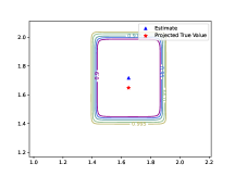
(a)

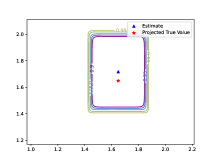
(b)

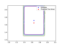
(c)

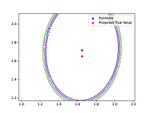
(d)

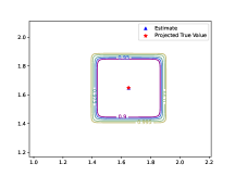
(e)

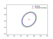
(f)

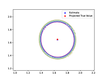
(g)

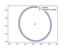
(h)

Figure 11: 2d slices of confidence regions passing through the point estimate with varying $d_{0}$ in the multivariate log-normal study.

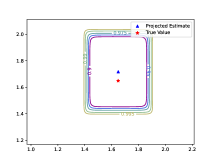
(a)

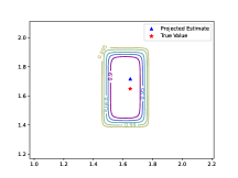
(b)

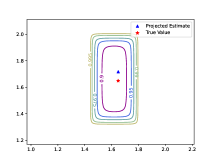
(c)

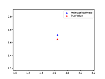
(d)

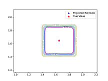
(e)

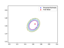
(f)

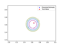
(g)

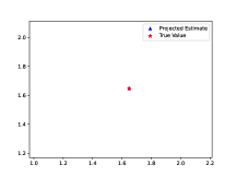
(h)

Figure 12: 2d slices of confidence regions passing through the true mean with varying $d_{0}$ in the multivariate log-normal study. Notably the true means are outside the confidence regions produced by Hotelling’s $T^{2}$ approach in this run.

4.3 Simulation Study with Log-Normal Samples

Our key assumption (3.3) does not require that the underlying data to be normal, since it appeals to the usual large-sample approximations. Nevertheless, the fact that the assumption (3.3) holds exactly for multivariate normal naturally raises the question if the good performance from the simulation studies in Section˜4.2 would be seen when the underlying data are not from normal. Our second simulation study is therefore designed to stress-test our method, by using a highly skewed distribution, log-normal, which is known to break common methods for constructing confidence intervals for the mean parameter, as in bootstrapping [Wood 1999]. Specifically, let $\boldsymbol{X}_{1},\dots,\boldsymbol{X}_{n}\in\mathbb{R}^{d}$ be i.i.d. samples from the distribution $\mathcal{N}(\boldsymbol{\theta},\boldsymbol{M}_{\rho})$, as described in Section˜4.2. Define $\boldsymbol{Y}_{i}=(\exp X_{i1},\ldots,\exp X_{id})^{\top}$, such that $Y_{ij}$ is marginally log-normally distributed. Our goal is to estimate the mean of $\boldsymbol{Y}_{i}$, with the true value being $e^{1/2}\mathbf{1}_{d}$ (when $\boldsymbol{\theta}=\boldsymbol{0}$).

Figure˜11 displays trends similar to those in Figure˜10: the size of the confidence regions decreases initially and then increases as $d_{0}$ grows. However, unlike the multivariate normal case, $95\%$ coverage is not guaranteed by using the nominal significance level of $0.05$. In our simulation studies over 2000 repetitions, we observe that the empirical coverage probabilities for $\boldsymbol{\theta}$ are $0.883$, $0.855$, $0.758$, and $0.322$ respectively with $d_{0}=1,5,25,100$. Therefore, our stress test does reveal the deterioration of our method when the underlying data are log-normal, even with $d_{0}=1$. However, relative to the dramatic loss of coverage by the standard Hotelling’s procedure $(d_{0}=d=1000)$, the deterioration is significantly less. Because our HCCT approach relies on the tail approximation, we anticipated that the deterioration may be less at the $0.01$ level. Indeed, the respective empirical coverages are $0.959$, $0.948$, $0.887$, and $0.502$. While labeling $96\%$ confidence regions (when $d_{0}=1$) as $99\%$ may be excusable as an approximation, advertising $50\%$ confidence regions (when $d_{0}=100$) as $99\%$ surely is deceiving.

We remark that the observed decay in validity as $d_{0}$ increases is likely due to the fact that, for a fixed sample size, the accuracy of Hotelling’s $T^{2}$ approximation in (3.3) diminishes as the dimension of the covariance matrix grows. This pattern is also evident in Figure˜12, which illustrates two-dimensional slices passing through the true mean rather than the empirical estimate in a single run. In particular, for $d_{0}=100$, the confidence regions implied by Hotelling’s $T^{2}$-test fail to contain the true mean altogether. General theoretical analysis for this phenomenon is another topic for further research.

5 Application to Network Meta-Analysis

5.1 Simultaneous Inference and Comparisons of Multiple Treatment Effects

In network meta-analysis, we aim to combine evidence from clinical trials involving $d+1$ intervention arms, consisting of $d$ active treatments and a placebo, which serves as the control arm. These treatments are represented as nodes in a network graph, with direct comparisons between treatments forming the edges. Trials may compare two or more arms. For multi-arm trials, we generate all possible pairwise comparisons between treatments and represent the trial as a set of two-arm studies. This decomposition allows each treatment comparison to be consistently evaluated across the network, enabling the synthesis of results from trials with varying designs and treatment combinations.

Our objective is to estimate the effects of $d$ active treatments across all studies and provide simultaneous confidence intervals for any pairwise treatment comparison. By simultaneous, we mean that the confidence intervals account for the uncertainty across all comparisons of interest, ensuring that the true effect sizes for all these pairs are captured with a specified overall confidence level. Let $\boldsymbol{\theta}$ denote the $d\times 1$ vector of treatment effects. We have data from $m\geq d$ two-arm studies, represented by $\widehat{\boldsymbol{\zeta}}=(\widehat{\zeta}_{1},\dots,\widehat{\zeta}_{m})^{\top}$, where $\widehat{\zeta}_{j}$ is the observed treatment effect in the $j$-th study (against the placebo), and the associated standard errors are $\sigma_{1},\dots,\sigma_{m}$. The fixed-effects model is given by $\widehat{\boldsymbol{\zeta}}=\boldsymbol{\Omega}\boldsymbol{\theta}+\boldsymbol{\epsilon}$ with $\boldsymbol{\epsilon}\sim\mathcal{N}(\boldsymbol{0},\boldsymbol{\Sigma})$, where $\boldsymbol{\Sigma}$ is an unknown covariance matrix, with diagonal entries $\sigma_{1}^{2},\dots,\sigma_{m}^{2}$. The design matrix $\boldsymbol{\Omega}=(\boldsymbol{\omega}_{1},\dots,\boldsymbol{\omega}_{m})^{\top}\in\mathbb{R}^{m\times d}$ encodes the structure of the trials, where row $\boldsymbol{\omega}_{j}^{\top}$ represents the design of the $j$-th study. For a study comparing treatment $\theta_{k}$ against the placebo, $\boldsymbol{\omega}_{j}$ has $\omega_{jk}=1$ and $\omega_{j\ell}=0$ for all $\ell\neq k$. For studies comparing two active treatments, say $\theta_{k_{1}}$ and $\theta_{k_{2}}$, we set $\omega_{jk_{1}}=1$, $\omega_{jk_{2}}=-1$, and $\omega_{j\ell}=0$ for all $\ell\neq k_{1},k_{2}$. We assume that the network graph is connected, ensuring that $\boldsymbol{\Omega}$ is of full rank $d$.

The traditional approach for estimating treatment effects in meta-analysis is to use the weighted least squares (WLS) estimator, assuming independence between different studies [Schwarzer et al. 2015]. The point estimator is given by $\small\normalsize\widehat{\boldsymbol{\theta}}=(\boldsymbol{\Omega}^{\top}\widehat{\boldsymbol{W}}\boldsymbol{\Omega})^{-1}\boldsymbol{\Omega}^{\top}\widehat{\boldsymbol{W}}\widehat{\boldsymbol{\zeta}},\small\normalsize$ where $\widehat{\boldsymbol{W}}=\operatorname{diag}\left(1/\widehat{\sigma}_{1}^{2},\dots,1/\widehat{\sigma}_{m}^{2}\right)$ is a diagonal matrix of inverse variance weights. Let $\boldsymbol{L}=(\boldsymbol{\Omega}^{\top}\widehat{\boldsymbol{W}}\boldsymbol{\Omega})^{-1}=(L_{ij})$. The variance for the $j$-th treatment effect is estimated by $L_{jj}$, and the variance for the comparison between the $i$-th and $j$-th treatments is given by $L_{ii}+L_{jj}-2L_{ij}$. Using these variance estimates, one can construct asymptotic confidence intervals for each comparison. To obtain simultaneous confidence intervals across all comparisons, traditionally a Bonferroni correction is applied to control the family-wise error rate. For multi-arm trials, where multiple two-arm studies are derived from a single experiment, one can modify the approach by using a block-diagonal structure for $\widehat{\boldsymbol{W}}$, with each block corresponds to the inverse of the estimated covariance matrix for the related two-arm studies. Such adjustments may require access to the original experimental data from the multi-arm trials.

In contrast to these traditional methods, we allow $\boldsymbol{\Sigma}$ to have arbitrary off-diagonal entries, accommodating essentially any valid dependence structure between studies (the theoretical conditions in Theorem˜2.4 are rather mild). Our approach only requires the estimated average treatment effects and their standard deviations from each study. The reasoning is straightforward: for each two-arm study, we have an estimate $\widehat{\zeta}_{j}\sim\mathcal{N}(\boldsymbol{\omega}_{j}^{\top}\boldsymbol{\theta},\sigma_{j}^{2})$, where $\boldsymbol{\omega}_{j}^{\top}$ is the $j$-th row of $\boldsymbol{\Omega}$. This leads to the same setting introduced in Section˜3.2, where $\boldsymbol{P}_{j}=\boldsymbol{\omega}_{j}^{\top}$ for $j=1,\dots,m$. Thus, we can immediately obtain point estimates, confidence regions, and simultaneous confidence intervals via HCCT.

Addressing dependence is crucial here, as dependence naturally arises when multi-arm studies are decomposed into two-arm comparisons or when there is overlap in datasets across studies. In particular, as demonstrated in Abbas-Aghababazadeh et al. [2023], dependence between studies is common in genetic studies.

5.2 Empirical Demonstrations

We illustrate the validity and utility of our approach by applying it to both semi-synthetic and real-world examples from Senn et al. [2013], which compared different treatments for controlling blood glucose levels in patients with diabetes, using a meta-analysis of 26 previous medical studies, including $25$ two-arm clinical trials and $1$ three-arm trial. The analysis involved $10$ treatments, consisting of $9$ different drugs (acar, benf, metf, migl, piog, rosi, sita, sulf, vild) and a placebo. This dataset is available in the R package netmeta [Schwarzer et al. 2015], and contains a total of $28$ two-way comparisons, with reported means and standard deviations of the differences in glucose outcome levels.

To validate our approach and compare it with the traditional WLS method in the context of dependent studies, we consider a semi-synthetic experiment. The design matrix remains identical to that of the real-world example mentioned above, but the underlying average treatment effects and covariance structure are generated as follows:

$$\boldsymbol{\theta} =(0,-0.5,-1,0,-0.5,-1,0,-0.5,-1)^{\top},$$

$$\boldsymbol{\Sigma} =(\sigma_{ij}),\quad\sigma_{ii}=0.01\ \text{ for }\ 1\leq i\leq 28,\quad\sigma_{ij}=0.01\rho\ \text{ for }\ i\neq j,$$

where $\rho=0,0.1,\dots,0.9$ is a hyperparameter controlling the dependence level between the studies.

Table˜4 presents the point estimates from WLS and HCCT in a single run with correlation levels $\rho=0,0.3,0.6,0.9$ respectively. Figure˜13 shows the coverage of simultaneous confidence intervals and their average width for $\theta_{1}$ and $\theta_{2}$ at varying dependence levels, based on $500$ replications. These simultaneous intervals ensure joint coverage across all comparisons between each active treatment and the placebo at the $95\%$ confidence level. Additionally, we adjust the significance level for WLS by manually increasing the quantile multiplier in calculating confidence intervals until approximately $95\%$ coverage is achieved under dependence, and plot the widths of the resulting intervals (labeled “WLS-MA”). Such a manual adjustment is not feasible in real applications, but it is included in our simulation both to ensure fair comparison of the power and to stress-test HCCT by pinning it against an impractical benchmark.

$\boldsymbol{\rho}$		$\widehat{\theta}_{1}$	$\widehat{\theta}_{2}$	$\widehat{\theta}_{3}$	$\widehat{\theta}_{4}$	$\widehat{\theta}_{5}$	$\widehat{\theta}_{6}$	$\widehat{\theta}_{7}$	$\widehat{\theta}_{8}$	$\widehat{\theta}_{9}$
0	WLS	.0277	-.561	-.994	.0962	-.510	-1.02	.137	-.496	-.949
	HCCT	.0349	-.567	-.985	.114	-.491	-1.02	.137	-.496	-.949
0.3	WLS	-.0334	-.558	-1.09	-.0927	-.662	-1.12	-.0570	-.430	-.898
	HCCT	-.0209	-.579	-1.09	-.0923	-.671	-1.12	-.0570	-.422	-.898
0.6	WLS	.0850	-.403	-.926	.113	-.450	-.949	-.0325	-.494	-1.01
	HCCT	.0857	-.411	-.928	.104	-.449	-.951	-.0325	-.497	-1.01
0.9	WLS	-.0741	-.679	-1.13	-.149	-.762	-1.18	-.205	-.501	-1.14
	HCCT	-.0666	-.682	-1.13	-.139	-.765	-1.19	-.205	-.501	-1.14
True Value $\boldsymbol{\theta}$		0	-.5	-1	0	-.5	-1	0	-.5	-1

Table 4: Average treatment effects against the placebo (simulation).

As seen in Table˜4, both WLS and HCCT produce point estimates that are reasonably close to the ground truth. However, Figure˜13 demonstrates that the simultaneous confidence intervals obtained from WLS, even with Bonferroni correction, deteriorate rapidly as the dependence between studies increases. This shows that the validity of WLS depends critically on the assumption of independence among studies.

In contrast, HCCT automatically accounts for the potential dependence between studies, ensuring that the procedure is valid. It does so using wider intervals, and their width increases as the dependence level $\rho$ increases. The fact that the WLS intervals remain narrower and are not affected by $\rho$ is responsible for its deterioration in terms of validity. This point is also reflected by the fact that once we manually adjust the WLS to achieve the correct coverage, the width of the WLS intervals becomes much larger and exceeds those produced by HCCT when $\rho$ increases above a threshold. This threshold apparently depends on the components of $\boldsymbol{\theta}$, about $\rho=0.5$ for $\theta_{1}$ and $\rho=0.2$ for $\theta_{2}$, suggesting that the search for an adaptive optimal choice will be a complex matter. Using HCCT by itself is simpler and has built-in resilience to the (unknown) value of $\rho$.

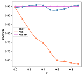
(a)

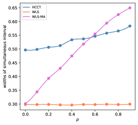
(b)

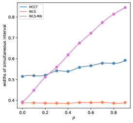
(c)

Figure 13: Coverage and width of simultaneous CIs (simulation).

Next, we consider the original real-world example, where we encounter the issue of empty confidence regions because of severe inconsistency in the studies. We adopt the sequential elimination approach justified in Section˜3.3, starting by including all studies. Once an empty solution is encountered, we can rank the studies according to an “outlier score", such as the generalized heterogeneity statistic [Schwarzer et al. 2015], $Q_{j}=\bigl{(}\widehat{\zeta}_{j}-\boldsymbol{\omega}_{j}^{\top}\widehat{\boldsymbol{\theta}}\bigr{)}^{2}/\widehat{\sigma}_{j}^{2},j=1,\ldots,m$ (or using the lower bound in (3.7)). We then give zero (or sufficiently small) weight to the study with the highest score and repeat our HCCT procedure (which may require resetting $P_{j}$’s to ensure they span $R^{d}$). If an empty-set solution still occurs, we repeat the procedure, until a nonempty solution is found – recall with $m=1$, the confidence region will always be nonempty.

In the blood glucose control example, two studies were removed based on our approach. The final point estimate from HCCT is quite close to that provided by WLS, as shown in Table˜5. However, the behavior of the simultaneous confidence intervals differs between the two methods. We visualize the widths of these intervals in the heatmaps (see Figure˜14). For WLS, the Bonferroni correction is applied to all pairwise comparisons, including those involving placebo.

From Figure˜14, we observe that the widths of simultaneous confidence intervals from HCCT are roughly comparable to those from WLS, though the former exhibit higher variability. Figure˜15 highlights a key limitation of the Bonferroni correction: the individual interval widths from WLS necessarily increase with the number of comparisons. This issue does not arise with our method, as individual comparisons are derived from projections of $d$-dimensional confidence regions. In this sense, WLS intervals with the largest Bonferroni corrections provide a more equitable comparison to the corresponding intervals obtained using HCCT. However, even these widest WLS intervals may still fall (significantly) short in ensuring the nominal coverage, when there are dependence across studies. In contrast, HCCT accounts for this dependence, and apparently it is able to do so without unduly widening the intervals, at least compared to those based on Bonferroni correction. It is yet another research direction to theoretically compare HCCT with Bonferroni correction in terms of both validity and power.

	acar	benf	metf	migl	piog	rosi	sita	sulf	vild
WLS	-0.827	-0.905	-1.11	-0.944	-1.07	-1.20	-0.57	-0.439	-0.7
HCCT	-0.806	-0.828	-1.01	-1.02	-1.02	-1.31	-0.57	-0.406	-0.7

Table 5: Average treatment effects against the placebo (real data).

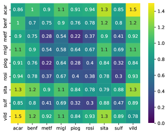
(a)

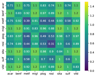
(b)

Figure 14: Widths of simultaneous confidence intervals for all comparisons.

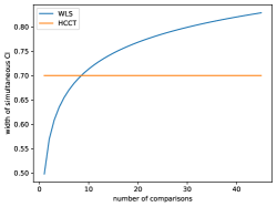
(a)

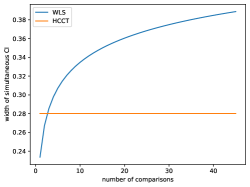
(b)

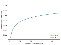
(c)

Figure 15: Widths of simultaneous CIs with increasing numbers of comparisons.

6 Reflections, Limitations, and Invitations

When two of us worked on proving the Drton-Xiao conjecture a decade ago, which ultimately led to the publication of Pillai and Meng [2016], we were driven purely by theoretical curiosity, as documented in Meng [2024]. We were very delighted by the discovery of the largely forgotten Cauchy combination result (1.1), which rendered us an elegant proof. But we didn’t realize its far-reaching theoretical and practical implications, other than the hunch that it might suggest that heavy marginal tails can overwhelm joint stochastic behaviors [Pillai and Meng 2016, Section 1]. We are therefore grateful to—and excited by—Liu and Xie [2020] and all the concurrent and subsequent articles as sampled in Section˜1 for developing the more versatile heavy-tail approximations based on Cauchy and other related combination schemes.

We are excited because of the potential of the heavy-tail approximations. Large-sample approximations have dominated the statistical theory and practice primarily because they largely free us from worrying about the infinite-dimensional distribution shapes, conceptually and computationally. In a similar vein, the heavy-tail approximations can liberate us from the burden of dealing with dependence structures as nuisance objects [Meng 2024]. As a proof-of-concept demonstration of possibilities generated by this liberation, we illustrate the divide-and-combine strategy in the simplest common applications of normal mean. But clearly the strategy can be tried on any estimation problem in any dimension where it is possible to conduct “lossless modularization", meaning that when all the modularized components are integrated, the information integrity (e.g., estimand identifiability) of the original problem is kept.

How to carry out such modularization most effectively is a sub-field in and of itself, and we imagine there are many lines of inquiries, depending on the inference problems at hand. There will be challenges such as with temporally or spatially dependent data. Even for the simpler problems discussed in this article, we do not claim any theoretical or practical optimality of our proposals—we only demonstrate their feasibility and improved competitiveness (against conventional benchmarks) brought in by the heavily right strategy. There are a host of theoretical, methodological, and computational open problems, such as optimal choices of dimensions for the sub-studies (and what are the suitable optimality criterion for balancing statistical and computational efficiency); the behaviors of the confidence regions when the dimension-reduction projections are random; finding useful error bounds on the difference between the actual and nominal coverages from the Half-Cauchy or Harmonic mean combinations; and finding effective algorithms to compute the confidence regions when the projections themselves are of considerable dimensions.

There are also many foundational questions raised by the “Cauchy surprise" and the subsequent work. Why can the dependence surrender to heavy marginal tails? Is that the real explanation or is there something more profound about stochastic behaviors that collectively we have failed to understand? Why heavily right is right? What would be an inferential principle that automatically prefers Half-Cauchy to Cauchy, because it prioritizes convexity as a desirable property? What are the consequences of having a $p$-value from a test statistic that does not lead to convex confidence regions?

With these and many more questions on our minds, we reiterate the invitations in previous sections to all interested parties to join us to explore this new paradigm of heavy-tail approximations for integrated dependent studies and especially for estimation in any dimension via the divide-and-combine strategy. Indeed, we will be more excited if all strategies, methods, and results presented in this article can be improved significantly.

Appendix A Exact Harmonic Mean P-Value

The combined test statistic in the harmonic mean method is defined as $T_{\textup{HMP}}=\sum_{j=1}^{m}\frac{w_{j}}{p_{j}}$. If $p_{j}$ is uniform in $[0,1]$, then $1/p_{j}$ follows the $\textup{Pareto}(1,1)$ distribution. As a reminder, the $\textup{Pareto}(\alpha,\mu)$ distribution has the following density function:

$$\small\normalsize f_{\textup{Pareto}}(x;\alpha,\mu)=\alpha\mu^{\alpha}x^{-1-\alpha}\mathbb{I}_{\{x\geq\mu\}}.\small\normalsize$$

The approach of harmonic mean p-value (HMP) was initially proposed by Good (1958) for combining independent $p$-values, and recently rediscovered by Wilson (2019) for dependent studies. However, they can only obtain the asymptotic distribution of the test statistics with $m\to\infty$ and $w_{1}=\dots=w_{m}=1/m$. We propose a numerical approach that could calculate the exact distribution with finite $m$ and allow for unequal weights. Next we introduce our numerical approach in computing the exact density and CDF for the weighted sum of i.i.d. $\textup{Pareto}(1,1)$ random variables. Similar to the proof of Theorem˜2.3, for $X_{j}\mathrel{\overset{\scalebox{0.6}{ i.i.d.}}{\scalebox{1.2}[1.0]{$\sim$}}}\textup{Pareto}(1,1)$ we can perform Laplace transform on $X_{j}-1$ and obtain the density function $f_{m}(x)$ by contour integration. The idea dates back to Ramsay (2006), and the following theorem is a modification of their main result, allowing unequal weights in the derivation.

Theorem A.1.

Let $f_{\textup{Pareto}}(x)=x^{-2}\ \mathbb{I}_{x\geq 1}$ be the density of the $\textup{Pareto}(1,1)$ distribution, and for non-negative weights $w_{1},\dots,w_{m}$ that sum up to $1$. Then the density $f_{\textup{Pareto},\boldsymbol{w}}(x)$ of the weighted sum of $\textup{Pareto}(1,1)$ variables $\sum_{j=1}^{m}w_{j}X_{j}$ can be written as

$$\small\normalsize f_{\textup{Pareto},\boldsymbol{w}}(x)=\frac{1}{2\pi i}\int_{0}^{\infty}e^{-xz}\Bigl{(}\prod_{j=1}^{m}\{-\operatorname{Ei}_{2}(w_{j}z)+i\pi w_{j}z\}-\prod_{j=1}^{m}\{-\operatorname{Ei}_{2}(w_{j}z)-i\pi w_{j}z\}\Bigr{)}\mathop{}\!\mathrm{d}z,\small\normalsize$$

where $\operatorname{Ei}_{2}(z)$ is the second-order exponential integral, whose convergent series is given by the following formula (Abramowitz and Stegun, 1968)

$$\small\normalsize\operatorname{Ei}_{2}(z)=-1+z(\log z+\gamma-1)+\sum_{j=2}^{\infty}\frac{z^{j}}{(j-1)j!}.\small\normalsize$$

Or it could be defined through the first-order exponential integral:

$$\small\normalsize\operatorname{Ei}_{2}(x):=x\operatorname{Ei}(x)-\exp(x),\quad\operatorname{Ei}(x):=-\int_{-x}^{\infty}\frac{e^{-\xi}}{\xi}\mathop{}\!\mathrm{d}\xi=\int_{-\infty}^{x}\frac{e^{\xi}}{\xi}\mathop{}\!\mathrm{d}\xi.\small\normalsize$$

Although the exponential integrals are pre-defined special function in the Python package SciPy, we cannot directly use it because $\operatorname{Ei}(x)$ is roughly of order $\exp(x)$, which causes overflow with large $x$ when doing numerical integration. In fact, we can overcome this issue using an accurate calculation of $\operatorname{Ei}(x)/\exp(x)$ for any $x\geq 0$. To solve this problem we consider the (faster) series expansion by Ramanujan:

$$\small\normalsize\operatorname{Ei}(x)=\gamma+\log x+\exp(x/2)\sum_{n=1}^{\infty}\frac{(-1)^{n-1}x^{n}}{n!2^{n-1}}\sum_{k=0}^{\lfloor(n-1)/2\rfloor}\frac{1}{2k+1},\small\normalsize$$

and divide each term by $\exp(x)$ to get

$$\frac{\operatorname{Ei}(x)}{\exp(x)}=(\gamma+\log x)\exp{(-x)}$$

$$\qquad+\sum_{n=1}^{\infty}(-1)^{n-1}\exp\Bigl{\{}n\log x-\sum_{j=1}^{n}\log j-(n-1)\log 2-\frac{x}{2}\Bigr{\}}\sum_{k=0}^{\lfloor(n-1)/2\rfloor}\frac{1}{2k+1}.\small\normalsize$$

Next, we derive the asymptotics with $m\to\infty$ and arbitrary $w_{1},\dots,w_{m}$.

Theorem A.2.

Consider a triangular array of weights $\{w_{j}^{(m)}\}_{m\geq 1,1\leq j\leq m}$ such that

• $w_{j}^{(m)}\geq 0$ for any $m\geq 1,1\leq j\leq m$;

• $\sum_{j=1}^{m}w_{j}^{(m)}=1$ for any $m\geq 1$;

• $\max_{j}w_{j}^{(m)}\to 0$ as $m\to\infty$.

Let $(X_{j})$ be a sequence of i.i.d. variables from $\textup{Pareto}(1,1)$. Then it holds that

$$\small\normalsize\sum_{j=1}^{m}w_{j}^{(m)}X_{j}-\Bigl{\{}-\sum_{j=1}^{m}w_{j}^{(m)}\log w_{j}^{(m)}+1-\gamma\Bigr{\}}\mathrel{\xrightarrow{\textup{d}}}S\Bigl{(}1,1,\frac{\pi}{2},0\Bigr{)}=\textup{Landau}\Bigl{(}0,\frac{\pi}{2}\Bigr{)},\small\normalsize$$

where $\gamma:=\lim_{m\to\infty}(\sum_{k=1}^{m}\frac{1}{k}-\log m)\approx 0.5772$ is the Euler–Mascheroni constant.

Finally, similar to Theorems˜3.1 and 3.2 we present a result on the convexity of confidence regions from EHMP, which has not been discovered in literature.

Theorem A.3.

For the harmonic mean method, i.e., $\nu\sim\textup{Pareto}(1,1)$, the solution set of (3.2) is a single (connected) finite interval. The solution set of (3.5) is convex in $\mathbb{R}^{d}$ as long as $k_{j}\geq d_{j}+1$ for all $j=1,\dots,m$ and bounded if the row vectors of $\{\boldsymbol{P}_{1},\dots,\boldsymbol{P}_{m}\}$ span $\mathbb{R}^{d}$.

$m$	$x$	PDF (Err)	Time (s)	Landau Approx	CDF (Err)	Time (s)	Landau Approx
2	2	.303993203 ($\pm$5E-9)	.150	.150080964	.362673464 ($\pm$2E-8)	.046	.433900891
	10	.012418123 ($\pm$2E-8)	.039	.014947778	.885277805 ($\pm$4E-9)	.035	.868002274
	50	.000432721 ($\pm$2E-9)	.049	.000471188	.979080976 ($\pm$7E-9)	.030	.978043335
10	4	.155679561 ($\pm$1E-9)	.039	.133578865	.492596674 ($\pm$2E-8)	.028	.489298321
	10	.019829249 ($\pm$3E-9)	.019	.021397821	.847965230 ($\pm$8E-9)	.040	.839184630
	50	.000491781 ($\pm$6E-9)	.023	.000505060	.977583372 ($\pm$1E-9)	.034	.977258199
100	2	.000000387 ($\pm$1E-8)	.445	.000554016	.000000015 ($\pm$4E-9)	.272	.000068807
	5	.191884746 ($\pm$1E-8)	.097	.179262887	.274570971 ($\pm$2E-8)	.096	.281827251
	10	.038837066 ($\pm$6E-9)	.097	.039487463	.774900747 ($\pm$8E-9)	.086	.771927461
	50	.000557767 ($\pm$2E-8)	.045	.000560181	.976086590 ($\pm$2E-9)	.045	.976033423
1000	4	.000009348 ($\pm$2E-8)	1.565	.000043914	.000000671 ($\pm$1E-9)	1.405	.000004086
	7	.182779813 ($\pm$1E-8)	.455	.180180123	.225626049 ($\pm$3E-9)	.501	.227272659
	10	.083072268 ($\pm$2E-8)	.337	.083192398	.639103576 ($\pm$2E-8)	.377	.638216812
	50	.000624345 ($\pm$2E-9)	.323	.000624742	.974679223 ($\pm$5E-9)	.317	.974671236

Table 6: Precision and runtime cost of EHMP with equal weights.

Appendix B Further Discussion for Section 2

B.1 Tail Independence and Copulas

Intuitively the condition in Theorem˜B.2 indicates that the dependence level between $X_{i}$ and $X_{j}$ in the tail is small. This is related to the notion of upper tail dependence coefficient in extreme value analysis (Sibuya, 1960; Ledford and Tawn, 1997; Joe, 1997; Schmidt, 2002; Draisma et al., 2004; Schmidt, 2005):

Definition B.1.

Let $\boldsymbol{X}=(X_{1},X_{2})^{\top}$ be a $2$-dimensional random vector. The upper tail dependence coefficient for $\boldsymbol{X}$ is defined as

$$\small\normalsize\lambda:= \lim_{v\to 0_{+}}\mathbb{P}\{X_{1}>F_{1}^{-1}(1-v)\mid X_{2}>F_{2}^{-1}(1-v)\}$$

$$= \lim_{v\to 0_{+}}\mathbb{P}\{X_{2}>F_{2}^{-1}(1-v)\mid X_{1}>F_{1}^{-1}(1-v)\}\small\normalsize$$

where the limit exists and $F_{1}^{-1},F_{2}^{-1}$ denotes the generalized inverse CDF of $X_{1},X_{2}$. We say that $\boldsymbol{X}=(X_{1},X_{2})^{\top}$ is tail independent if $\lambda=0$.

In fact, Theorem˜2.4 could be restated using the conditions similar to but slightly stronger than tail independence, the proof of which is provided in Appendix˜C:

Theorem B.2.

For fixed $m$ if there exists a function $r(\cdot)$ such that $r(v)/v\to\infty$ as $v\to 0_{+}$ and

$$\small\normalsize\lim_{v\to 0_{+}}\max_{1\leq i\neq j\leq m}\mathbb{P}\bigl{[}X_{i}>F_{i}^{-1}\{1-r(v)\}\mid X_{j}>F_{j}^{-1}(1-v)\bigr{]}=0,\small\normalsize$$ (B.1)

then the Half-Cauchy combination test satisfies

$$\small\normalsize\lim_{x\to\infty}\frac{\mathbb{P}(T_{\textup{HCCT}}>x)}{1-F_{\textup{HC},\boldsymbol{w}}(x)}=\lim_{x\to\infty}\frac{\mathbb{P}(T_{\textup{HCCT}}>x)}{1-\frac{2}{\pi}\arctan(x)}=1,\small\normalsize$$ (B.2)

where $F_{\textup{HC},\boldsymbol{w}}(x)$ denotes CDF of the test statistic under independence.

For diverging $m$, suppose $\max_{1\leq i\neq j\leq m}{w_{i}/w_{j}}=\mathcal{O}(1)$. If there exists $v_{m}$ and $r(\cdot)$ such that $v_{m}\to 0_{+}$ and $r(v_{m})/v_{m}\to\infty$ as $m\to\infty$ and that

$$\small\normalsize\lim_{m\to\infty}m^{2}\max_{1\leq i\neq j\leq m}\mathbb{P}\bigl{[}X_{i}>F_{i}^{-1}\{1-r(v_{m})\}\mid X_{j}>F_{j}^{-1}(1-v_{m})\bigr{]}=0,\small\normalsize$$ (B.3)

then the Half-Cauchy combination test satisfies that

$$\small\normalsize\lim_{m\to\infty}\frac{\mathbb{P}(T_{\textup{HCCT}}>x_{m})}{1-F_{\textup{HC},\boldsymbol{w}}(x_{m})}=\lim_{m\to\infty}\frac{\mathbb{P}(T_{\textup{HCCT}}>x_{m})}{1-\frac{2}{\pi}\arctan(x_{m})}=1\small\normalsize$$ (B.4)

for any $x_{m}$ such that $\liminf_{m\to\infty}x_{m}v_{m}>0$.

As implied by Corollary˜2.5 the bivariate normal distribution is tail independent. However, there are other distributions that are tail dependent including the bivariate $t$-distribution as shown in Schmidt (2002). Its tail dependence coefficient has been extended to multivariate cases and extensively studied in Frahm (2006); Chan and Li (2007).

Moreover, the concept of copulas is an important tool in studying tail independence (Embrechts et al., 2001). Consider a random vector $\boldsymbol{X}=(X_{1},\dots,X_{m})^{\top}$. Suppose its marginal CDFs $F_{j}(x)=\mathbb{P}(X_{j}\leq x)$ are continuous. By applying the probability integral transform to each component, the random vector

$$\small\normalsize(U_{1},\dots,U_{m})=\{F_{1}(X_{1}),\dots,F_{m}(X_{m})\}\small\normalsize$$

has marginals that are uniformly distributed on the interval $[0,1]$.

Definition B.3 (Copula).

The copula of $\boldsymbol{X}$ is defined as the joint cumulative distribution of $(U_{1},\dots,U_{m})$ given by

$$\small\normalsize C(u_{1},\dots,u_{m})=\mathbb{P}(U_{1}\leq u_{1},\dots,U_{m}\leq u_{m}).\small\normalsize$$

Sklar’s theorem (Sklar, 1959; Durante et al., 2013) shows that every multivariate CDF of a random vector $\boldsymbol{X}$ can be expressed in terms of its marginals $F_{j}(x_{j})$ ($j=1,\dots,m$) and a copula $C$, i.e.,

$$\small\normalsize H(x_{1},\dots,x_{m})=\mathbb{P}(X_{1}\leq x_{1},\dots,X_{m}\leq x_{m})=C\{F_{1}(x_{1}),\dots,F_{m}(x_{m})\}.\small\normalsize$$

In other words, the copula contains all information on the dependence structure between the components of $(X_{1},\dots,X_{m})$ whereas the marginal CDFs contain all information on the marginal distributions of $X_{j}$.

As shown in Long et al. (2023) the assumption of Theorem˜2.4 is satisfied by a number of commonly-used bivariate copulas, including but not limited to the independence copula and the normal copula:

• Independence Copula:

  $$\small\normalsize C(u,v)=uv;\small\normalsize$$

• Normal Copula:

  $$\small\normalsize\textstyle C(u,v)=\frac{1}{2\pi\sqrt{1-\rho}}\int_{-\infty}^{\Phi^{-1}(u)}\int_{-\infty}^{\Phi^{-1}(v)}\exp\biggl{\{}-\frac{x^{2}-2\rho xy+y^{2}}{2(1-\rho^{2})}\biggr{\}}\mathop{}\!\mathrm{d}x\mathop{}\!\mathrm{d}y,\small\normalsize$$

  where $\rho$ is the correlation between the two normal variables;

• Survival Copula:

  $$\small\normalsize C(u,v)=uv\exp(-\theta\log u\log v),\quad\theta\in[0,1];\small\normalsize$$

• Farlie–Gumbel–Morgenstern (FGM) Copula:

  $$\small\normalsize C(u,v)=uv\{1+\theta(1-u)(1-v)\},\quad\theta\in[-1,1];\small\normalsize$$

• Cuadras–Augé Copula:

  $$\small\normalsize C(u,v)=(\min\{u,v\})^{\theta}(uv)^{1-\theta},\quad\theta\in[0,1];\small\normalsize$$

• Ali–Mikhail–Haq (AMH) Copula:

  $$\small\normalsize\textstyle C(u,v)=\frac{uv}{1-\theta(1-u)(1-v)},\quad\theta\in[0,1].\small\normalsize$$

To illustrate, we show more simulation results on the validity of HCCT using dependency structures other than the multivariate normal of Section˜2.5. First, we check the FGM and AMH copulas as mentioned above using the following setup from (Long et al., 2023):

• FGM copula mixed with product copula model:

  $$\small\normalsize(p_{j},p_{j+1})^{\top}\sim C(u_{j},v_{j+1})=\begin{cases}u_{j}v_{j+1}\bigl{\{}1+\theta(1-u_{j})(1-v_{j+1})\bigr{\}}&j=1,3,\dots,2\lfloor m/2\rfloor-1\\ u_{j}v_{j+1}&\text{else}\end{cases},\small\normalsize$$

• AMH copula mixed with product copula model:

  $$\small\normalsize(p_{j},p_{j+1})^{\top}\sim C(u_{j},v_{j+1})=\begin{cases}\frac{u_{j}v_{j+1}}{1-\theta(1-u_{j})(1-v_{j+1})}&j=1,3,\dots,2\lfloor m/2\rfloor-1\\ u_{j}v_{j+1}&\text{else}\end{cases}.\small\normalsize$$

The p-values are generated from the null hypothesis based on the above two models with $m=500$. Figure˜16 reports the false positive rate from $10000$ runs for HCCT and the Fisher’s combination test in these two settings. We can see that the combination test has roughly the correct size for HCCT while the actual size for Fisher’s combination test changes monotonously with the hyperparameter $\theta$. As a result the Fisher’s combination test is less valid with large positive $\theta$’s.

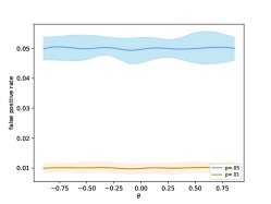
(a)

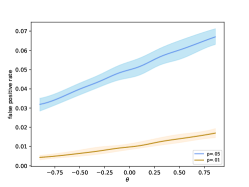
(b)

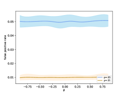
(c)

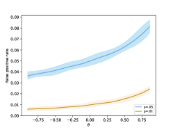
(d)

Figure 16: Comparison of false positive rates with AMH and FGM copulas.

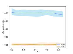
(a)

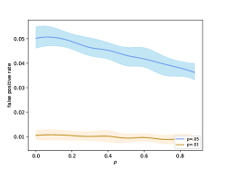
(b)

Figure 17: False positive rates of HCCT with multivariate $t$ copulas.

Next we consider replacing the normal distribution in Section˜2.5 by the multivariate $t$-distribution $t_{m,k}(\boldsymbol{\theta},\boldsymbol{\Sigma})$ with degrees of freedom $k=10$ and dimension $m=500$, the density of which is given by

$$\small\normalsize\frac{\Gamma\{(k+m)/2\}}{\Gamma(k/2)k^{m/2}\pi^{m/2}|\boldsymbol{\Sigma}|^{1/2}}\left\{1+\frac{1}{k}(\boldsymbol{x}-\boldsymbol{\theta})^{\mathrm{T}}\boldsymbol{\Sigma}^{-1}(\boldsymbol{x}-\boldsymbol{\theta})\right\}^{-(k+m)/2}.\small\normalsize$$

The individual p-values here are calculated from the tail probabilities of those marginal Student’s $t$-distributions with degrees of freedom $k=10$. We set $\boldsymbol{\theta}=\boldsymbol{0}$ under the null and compute the false positive rates from $10000$ runs with $\boldsymbol{\Sigma}$ being either AR-$1$ correlation or equi-correlation matrices as defined in Section˜2.5. The results are shown in Figure˜17. We can see that the HCCT is almost always of the correct size with AR-$1$ correlations and is slightly conservative with equi-correlations as $\rho$ grows.

B.2 Sensitivity to Large $p$-Values & Heavily Right Strategy

In global testing we care mostly about the small $p$-values and would like the combined $p$-values to be insensitive to large individual ones. However, as mentioned in Section˜1, the Cauchy combination test is quite sensitive to large $p_{j}$’s and does not address this concern well enough. In this section we aim to present the comparison of these combination tests in terms of sensitivity to large $p$-values.

$p$-values	Fisher	Stouffer	Bonferroni	CCT	CAtr	HCCT	EHMP
(.02, .03, .96)	.021	.104	.060	.051	.051	.039	.039
(.02, .03, .98)	.021	.139	.060	.088	.088	.039	.039
(.02, .03, .99)	.021	.177	.060	.837	.837	.039	.039
(.015, .9, .96)	.192	.691	.045	.091	.091	.050	.049
(.02, .02, .8, .98)	.040	.272	.080	.086	.086	.045	.045
(.01, .05, .3, .5, .99)	.040	.166	.050	.197	.197	.046	.046

Table 7: Examples of $p$-value combinations.

Table˜7 gives some tuples of $p$-values where it is more reasonable to reject the global null at significance level $0.05$ yet several previous approaches including CCT fail to do so because of their sensitivity to large $p_{j}$’s. Our proposed Half-Cauchy combination test (HCCT) and exact harmonic mean $p$-value (EHMP) along with the Fisher’s test and Bonferroni correction perform well in these extreme cases while the Stouffer’s Z-score test, CCT, and CAtr do not work as expected.

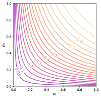
(a)

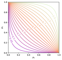
(b)

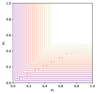
(c)

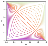
(d)

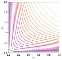
(e)

(f)

Figure 18: Combining two $p$-values with equal weights.

Figure˜18 shows the contour plot when we combine two $p$-values. We can see that for the Stouffer’s Z-score test and CCT, the contour lines get close together near the point $(1,0)$ in both $p_{1}$ and $p_{2}$ directions, which signifies that the combined $p$-value is sensitive to both $p_{1}$ and $p_{2}$. However, for the other approaches, the contour lines are close in the $p_{2}$ direction around $(1,0)$ but are at a distance away from one another in the $p_{1}$ direction, meaning that the combined $p$-value is sensitive to the smaller $p_{2}$ but insensitive to the larger $p_{1}$.

Figure˜2 reveals a key observation that problematic large $p_{j}$ values are mapped to the negative tail of the Cauchy (or normal) distribution when calculating scores for CCT (or the Stouffer’s Z-score test). Specifically, if a $p_{j}$ is close to one, the corresponding component $\cot(p_{j}\pi)$ in (2.2) will be far below zero, making it harder to reject the global null. This sensitivity to large $p_{j}$ values arises because both the Cauchy and normal distributions have equally heavy tails on both sides, canceling out the impact of significant small $p$-values. A potential remedy is to use a distribution $\nu$ with a heavier right tail than the negative tail. In the stable family $S(\alpha,\beta,c,\mu)$, this imbalance is controlled by the skewness parameter $\beta\in[-1,1]$, where a larger $\beta$ gives a relatively heavier right tail. Ideally, we select $\nu$ attracted to $S(\alpha,\beta,c,\mu)$ with $\beta=1$.

Since the previous subsection demonstrated that $\alpha=1$ is optimal for balancing validity and power under dependence, we select $\nu$ from distributions attracted to the Landau family (with $\alpha=\beta=1$). Examples from this class include $\text{Pareto}(1,1)$, left-truncated or winsorized Cauchy, and the Landau family itself. Moreover, for a small number of studies, if truncation threshold is far below $0$, the left-truncated or winsorized Cauchy methods of Gui et al. (2023); Fang et al. (2023) are still sensitive to large $p$-values (see Table˜7). Finally, we will show in the next section that the Half-Cauchy and $\text{Pareto}(1,1)$ are the only two among all these choices that lead to connected confidence regions when we invert the combination test.

Appendix C Proofs for Section 2

Proof of Theorem˜2.3.

For complex $z\in\mathbb{C}$ such that $\operatorname{Re}[z]>0$, the Laplace transform of the Half-Cauchy density is given by the following formula (Diédhiou, 1998):

$$\small\normalsize f^{\ast}_{\textup{HC}}(z)=\frac{2}{\pi}\int_{0}^{+\infty}\frac{e^{-xz}}{1+x^{2}}\mathop{}\!\mathrm{d}x=-\frac{2}{\pi}\{\sin(z)\operatorname{ci}(z)+\cos(z)\operatorname{si}(z)\}.\small\normalsize$$

Through analytic continuation $\operatorname{si}(z)$ can be extended to $\mathbb{C}$ while $\operatorname{ci}(z)$ can be extended to the Riemann surface of $\log z$ with the origin being the logarithmic branch point. Thus, $f^{\ast}(z)$ can also be extended to the Riemann surface of $\log z$.

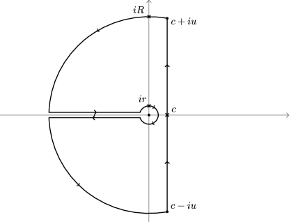
Figure 19: Contour integration.

Note that by property of Laplace transform, we have

$$\small\normalsize f_{\textup{HC},\boldsymbol{w}}^{\ast}(z)=\prod_{j=1}^{m}f_{\textup{HC}}^{\ast}(w_{j}z)=\Bigl{(}-\frac{2}{\pi}\Bigr{)}^{m}\prod_{j=1}^{m}\bigl{\{}\sin(w_{j}z)\operatorname{ci}(w_{j}z)+\cos(w_{j}z)\operatorname{si}(w_{j}z)\bigr{\}},\small\normalsize$$

and the inversion of $f_{\textup{HC},\boldsymbol{w}}^{\ast}(z)$ is obtained as the Bromwich integral (Bellman et al., 1966)

$$\small\normalsize f_{\textup{HC},\boldsymbol{w}}(x)=\frac{1}{2\pi i}\int_{c-i\infty}^{c+i\infty}e^{xz}f_{\textup{HC},\boldsymbol{w}}^{\ast}(z)\mathop{}\!\mathrm{d}z,\qquad x>0,\small\normalsize$$

where $c>0$ is any constant large enough so that all of the singularities of $f_{\textup{HC},\boldsymbol{w}}^{\ast}(z)$ lie to the left of the vertical line $\operatorname{Re}[z]=c$. (In our case the only singularity is $0$ and $c$ can be any positive real number.) Thus, we choose the logarithmic branch cut along the negative real axis ending at the branch point $0$ for the Riemann surface of $\log z$. Then $\operatorname{ci}(z)$ is analytic on the branch $\mathbb{C}\backslash\mathbb{R}_{\leq 0}$ and the Bromwich integral can be evaluated as a part of the integral in the counter-clockwise direction around the deformed contour $\Omega$ consisting of

• The vertical line $c+iy$ where $y$ goes from $-u$ to $u$ such that $R=\sqrt{c^{2}+u^{2}}$ is large;

• The semicircle with radius $R$, centered at the origin, lying to the left of the vertical line $\operatorname{Re}[z]=c$, and extended to connect the points $c\pm iu$;

• The line from $-R$ to $-r$ lying above the branch cut along the negative real axis;

• The line from $-r$ to $-R$ below the branch cut;

• The circle about the origin with a small radius $r\ll c$.

As $\sin z\operatorname{ci}(z)+\cos z\operatorname{si}(z)$ is analytic in $\Omega$, it follows from the Cauchy’s integral theorem that

$$\small\normalsize\frac{1}{2\pi i}\int_{\Omega}e^{xz}f_{\textup{HC},\boldsymbol{w}}^{\ast}(z)\mathop{}\!\mathrm{d}z=\frac{1}{2\pi i}\Bigl{(}-\frac{2}{\pi}\Bigr{)}^{m}\int_{\Omega}e^{xz}\prod_{j=1}^{m}\bigl{\{}\sin(w_{j}z)\operatorname{ci}(w_{j}z)+\cos(w_{j}z)\operatorname{si}(w_{j}z)\bigr{\}}=0,\small\normalsize$$

as $r\to 0,R\to\infty$. By Abramowitz and Stegun (1968) we can check that $\sin z\operatorname{ci}(z)+\cos z\operatorname{si}(z)=\mathcal{O}(1/z)$ as $\lvert z\rvert\to\infty$. Noting that for any fixed $x>0$

$$\small\normalsize\lvert e^{xz}\rvert=e^{x\operatorname{Re}[z]}\leq e^{cx}<\infty,\small\normalsize$$

the contribution from the large semicircle is zero as $R\to\infty$. Likewise, we can check that $\sin z\operatorname{ci}(z)+\cos z\operatorname{si}(z)=-\frac{\pi}{2}+\mathcal{O}(z\log z)$ and the contribution from the small circle is also zero as $r\to 0$. Thus, we have

$$\small\normalsize f_{\textup{HC},\boldsymbol{w}}(x)=\frac{1}{2\pi i}\int_{0}^{\infty}e^{-xz}\bigl{\{}f_{\textup{HC},\boldsymbol{w}}^{\ast}(ze^{-i\pi_{-}})-f_{\textup{HC},\boldsymbol{w}}^{\ast}(ze^{i\pi_{-}})\bigr{\}}\mathop{}\!\mathrm{d}z.\small\normalsize$$ (C.1)

Now for $z>0$ we have

$$\small\normalsize f_{\textup{HC}}^{\ast}(ze^{\pm i\pi_{-}}) =\frac{2}{\pi}\{\sin(z)\operatorname{ci}(z)+\cos(z)\operatorname{si}(z)\}+2\cos(z)\mp 2i\sin(z)$$

$$=-f_{\textup{HC}}^{\ast}(z)+2\cos(z)\mp 2i\sin(z).\small\normalsize$$

Thus, we have

$$\small\normalsize f_{\textup{HC},\boldsymbol{w}}(x)= \frac{1}{2\pi i}\int_{0}^{\infty}e^{-xz}\Bigl{[}\prod_{j=1}^{m}\{-f_{\textup{HC}}^{\ast}(w_{j}z)+2\cos(w_{j}z)+2i\sin(w_{j}z)\}$$

$$-\prod_{j=1}^{m}\{-f_{\textup{HC}}^{\ast}(w_{j}z)+2\cos(w_{j}z)-2i\sin(w_{j}z)\}\Bigr{]}\mathop{}\!\mathrm{d}z.\small\normalsize$$

∎

In order to show Theorem˜2.1, we present the generalized central limit theorem. The following version is from Gnedenko and Kolmogorov (1954).

Lemma C.1 (Generalized CLT).

A distribution with CDF $F(t)$ belongs to the domain of attraction of a normal distribution if and only if as $t\to\infty$

$$\small\normalsize\frac{t^{2}\int_{\lvert x\rvert>t}\mathop{}\!\mathrm{d}F(x)}{\int_{\lvert x\rvert<t}x^{2}\mathop{}\!\mathrm{d}F(x)}\to 0.\small\normalsize$$

The distribution with CDF $F(t)$ belongs to the domain of attraction of a stable distribution $S(\alpha,\beta,c,\mu)$ with the stability parameter $\alpha$ ($0<\alpha<2$) if and only if

$$\small\normalsize\lim_{t\to\infty}\frac{F(-t)}{1-F(t)}=\frac{1-\beta}{1+\beta}\in[0,\infty],\quad\lim_{t\to\infty}\frac{F(-t)+1-F(t)}{F(-kt)+1-F(kt)}=k^{\alpha}\quad\forall k>0.\small\normalsize$$

In particular, we have that

$$\small\normalsize\frac{1}{B_{n}}\sum_{i=1}^{n}X_{i}-A_{n}\mathrel{\xrightarrow{\textup{d}}}S(\alpha,\beta,c,\mu)\small\normalsize$$

where $B_{n}$ satisfies

$$\small\normalsize\lim_{k\to\infty}k\{F(-B_{k}t)+1-F(B_{k}t)\}=\frac{c^{\prime}}{t^{\alpha}}\quad\forall t>0,\small\normalsize$$

for some $c^{\prime}>0$ determined by $B_{n},\alpha$ and $c$.

The following lemma is a direct corollary of the main result in Shintani and Umeno (2018).

Lemma C.2.

Consider a triangular array of weights $(w_{j})_{n\geq 1,1\leq j\leq n}$ such that

• $w_{j}\geq 0$ for any $n\geq 1,1\leq j\leq n$;

• $\sum_{j=1}^{n}w_{j}=1$ for any $n\geq 1$;

• $\max_{j}w_{j}\to 0$ as $n\to\infty$.

Let $(X_{j})$ be a sequence of i.i.d. variables from a distribution $\nu$ with density $f(t)$ satisfying that

$$\small\normalsize f(t)\simeq\begin{cases}c_{1}/\lvert t\rvert^{\alpha+1}&\text{as }t\to-\infty\\ c_{2}/t^{\alpha+1}&\text{as }t\to\infty,\end{cases}\small\normalsize$$ (C.2)

for some $c_{1},c_{2}\geq 0$, $c_{1}+c_{2}>0$. Then we have

$$\small\normalsize\frac{1}{\bigl{(}\sum_{i=1}^{n}w_{i}^{\alpha}\bigr{)}^{\frac{1}{\alpha}}}\left(\sum_{j=1}^{n}w_{j}X_{j}-A_{n}\right)\mathrel{\xrightarrow{\textup{d}}}S(\alpha,\beta,c,0),\small\normalsize$$

where $\beta$ and $c$ are determined by

$$\small\normalsize\beta=\frac{c_{2}-c_{1}}{c_{1}+c_{2}},\quad c=\Bigl{\{}\frac{\pi(c_{1}+c_{2})}{2\alpha\sin\bigl{(}\frac{\pi\alpha}{2}\bigr{)}\Gamma(\alpha)}\Bigr{\}}^{\frac{1}{\alpha}},\small\normalsize$$ (C.3)

and $A_{n}$ is given by

$$\small\normalsize A_{n}=\begin{cases}0&\text{if }0<\alpha<1\\ \sum_{j=1}^{n}\operatorname{Im}\left[\log\phi_{X_{1}}\bigl{\{}w_{j}^{(n)}\bigr{\}}\right]&\text{if }\alpha=1\\ \mathbb{E}(X_{1})&\text{if }1<\alpha<2,\end{cases}\small\normalsize$$

where $\phi_{X}(\cdot)$ denotes that characteristic function of $X$ and $\operatorname{Im}$ gives the imaginery part of a complex number.

Now we are ready to prove Theorem˜2.1.

Proof of Theorem˜2.1.

Applying Lemma˜C.2 for the standard Half-Cauchy we have $\beta=c=1$. Now we compute $A_{m}$.

$$A_{m}=\operatorname{Im}\left[\sum_{j=1}^{m}\log\left\{\int_{0}^{\infty}\frac{2\cos(w_{j}x)}{\pi(1+x^{2})}\mathop{}\!\mathrm{d}x+i\int_{0}^{\infty}\frac{2\sin(w_{j}x)}{\pi(1+x^{2})}\mathop{}\!\mathrm{d}x\right\}\right]=\sum_{j=1}^{m}\theta_{j},$$ (C.4)

where

$$\sin(\theta_{j})=\int_{0}^{\infty}\frac{2\sin(w_{j}x)}{\pi(1+x^{2})}\mathop{}\!\mathrm{d}x,\quad\cos(\theta_{j})=\int_{0}^{\infty}\frac{2\cos(w_{j}x)}{\pi(1+x^{2})}\mathop{}\!\mathrm{d}x=e^{-w_{j}},\quad\tan(\theta_{j})= \int_{0}^{\infty}\frac{2\sin(w_{j}x)}{e^{w_{j}}\pi(1+x^{2})}\mathop{}\!\mathrm{d}x.$$

Here we have used eq. 3.766.2 of Gradshteyn and Ryzhik (2014) for $\cos(\theta_{j})$.

Next we deal with $\int_{0}^{\infty}\frac{\sin(ax)}{1+x^{2}}\mathop{}\!\mathrm{d}x$. Eq. 3.766.1 of Gradshteyn and Ryzhik (2014) shows that for any real number $a\in\mathbb{R}$ and $\mu\in(-1,1)\cup(1,3)$

$$\int_{0}^{\infty}\frac{x^{\mu-1}\sin(ax)}{1+x^{2}}\mathop{}\!\mathrm{d}x$$

$$= \frac{\pi\sinh(a)}{2\cos\left(\frac{\mu\pi}{2}\right)}+\frac{1}{2}\sin\left(\frac{\mu\pi}{2}\right)\Gamma(\mu)\left\{e^{-a-i\pi(1-\mu)}\gamma(1-\mu,-a)-e^{a}\gamma(1-\mu,a)\right\},$$ (C.5)

where $\Gamma(\cdot)$ is the (complete) gamma function and $\gamma(\cdot,\cdot)$ is the lower incomplete gamma function. They are defined as

$$\Gamma(s)=\int_{0}^{\infty}t^{s-1}e^{-t}\mathop{}\!\mathrm{d}t,\quad\gamma(s,x)=\int_{0}^{x}t^{s-1}e^{-t}\mathop{}\!\mathrm{d}t,$$

and can be extended to almost all combinations of complex $s$ and $x$. Note that the right hand side of (C) is not defined at $\mu=1$ but we show that $\mu=1$ is a removable discontinuity.

By Amore (2005) we have the following expansion for any $a\neq 0$

$$\gamma(x,a)=\frac{1}{x}+\{-\Gamma(0,a)-\gamma\}+\mathcal{O}(x),$$

where $\gamma$ is the Euler–Mascheroni constant, and $\Gamma(\cdot,\cdot)$ is the upper incomplete gamma function defined as

$$\Gamma(s,x)=\Gamma(s)-\gamma(s,x).$$

Thus, (C) can be rewritten as $I+II+\mathcal{O}(1-\mu)$ where

$$I: =\frac{\pi\sinh(a)}{2\cos\left(\frac{\mu\pi}{2}\right)}+\frac{1}{2}\sin\left(\frac{\mu\pi}{2}\right)\Gamma(\mu)\frac{e^{-a-i\pi(1-\mu)}-e^{a}}{1-\mu}$$

$$=\frac{\pi(e^{a}-e^{-a})}{4\sin\left\{\frac{\pi}{2}(1-\mu)\right\}}+\frac{1}{2}\sin\left(\frac{\mu\pi}{2}\right)\Gamma(\mu)\frac{e^{-a-i\pi(1-\mu)}-e^{a}}{1-\mu}$$

$$=\frac{\pi(e^{a}-e^{-a})}{4\sin\left\{\frac{\pi}{2}(1-\mu)\right\}}+\frac{1}{2}\sin\left(\frac{\mu\pi}{2}\right)\Gamma(\mu)$$

$$\qquad\frac{e^{-a}(\cos\{(1-\mu)\pi\}-1)+(e^{-a}-e^{a})-e^{-a}\sin\{(1-\mu)\pi\}}{1-\mu}$$

$$=\frac{e^{a}-e^{-a}}{2(1-\mu)}\left\{1-\sin\left(\frac{\mu\pi}{2}\right)\Gamma(\mu)\right\}-\frac{1}{2}e^{-a}\pi i+\mathcal{O}(1-\mu)$$

$$\overset{(*)}{=}-\frac{e^{a}-e^{-a}}{2}\gamma-\frac{1}{2}e^{-a}\pi i+\mathcal{O}(1-\mu),$$

and

$$II: =\frac{1}{2}\sin\left(\frac{\mu\pi}{2}\right)\Gamma(\mu)\left(e^{-a-i\pi(1-\mu)}\{-\Gamma(0,-a)-\gamma\}-e^{a}\{-\Gamma(0,a)-\gamma\}\right)$$

$$=\frac{1}{2}\left(e^{-a}\{-\Gamma(0,-a)-\gamma\}-e^{a}\{-\Gamma(0,a)-\gamma\}\right)+\mathcal{O}(1-\mu).$$

Note that $(*)$ is obtained by applying L’Hôpital’s rule:

$$\lim_{\mu\to 1}\frac{1-\sin\left(\frac{\mu\pi}{2}\right)\Gamma(\mu)}{1-\mu}=\lim_{\mu\to 1}\frac{-\frac{\pi}{2}\cos\left(\frac{\mu\pi}{2}\right)\Gamma(\mu)-\sin\left(\frac{\mu\pi}{2}\right)\Gamma^{\prime}(\mu)}{-1}=-\Gamma^{\prime}(1)=-\gamma.$$

Now by Amore (2005) again we have

$$\Gamma(0,a)=-\log a-\gamma+a+\mathcal{O}(a^{2}).$$

By Lebesgue’s dominated convergence theorem we have

$$\int_{0}^{\infty}\frac{\sin(ax)}{1+x^{2}}\mathop{}\!\mathrm{d}x=\lim_{\mu\to 1}\int_{0}^{\infty}\frac{x^{\mu-1}\sin(ax)}{1+x^{2}}\mathop{}\!\mathrm{d}x$$

$$= -\frac{e^{a}-e^{-a}}{2}\gamma-\frac{1}{2}e^{-a}\pi i+\frac{1}{2}\left(e^{-a}\{-\Gamma(0,-a)-\gamma\}-e^{a}\{-\Gamma(0,a)-\gamma\}\right)$$

$$= -\frac{e^{a}-e^{-a}}{2}\gamma+\frac{1}{2}\left\{e^{-a}(a+\log a)+e^{a}(a-\log a)\right\}+\mathcal{O}(a^{2})$$

$$= a\cosh(a)(1-\gamma)-a\log a\frac{\sinh(a)}{a}+\mathcal{O}(a^{2})$$

$$= a(1-\gamma)-a\log a+\mathcal{O}(a^{2}\log a).$$

Substitute this in (C.4), we get

$$\lim_{m\to\infty}\Bigl{(}A_{m}+\frac{2}{\pi}\sum_{j=1}^{m}w_{j}\log w_{j}\Bigr{)}$$

$$= \lim_{m\to\infty}\sum_{j=1}^{m}\left\{\int_{0}^{\infty}\frac{2\sin w_{j}x}{e^{w_{j}}\pi(1+x^{2})}\mathop{}\!\mathrm{d}x+\frac{2}{\pi}w_{j}\log w_{j}\right\}+\lim_{m\to\infty}\mathcal{O}\left[\sum_{j=1}^{m}\left\{\int_{0}^{\infty}\frac{2\sin w_{j}x}{e^{w_{j}}\pi(1+x^{2})}\mathop{}\!\mathrm{d}x\right\}\right]$$

$$= \lim_{m\to\infty}\left\{\frac{2}{\pi}(1-\gamma)\sum_{j=1}^{m}w_{j}+\mathcal{O}\Bigl{(}\sum_{j=1}^{\infty}w_{j}^{2}\log w_{j}\Bigr{)}\right\}+\lim_{m\to\infty}\mathcal{O}\left(\frac{2}{\pi}\sum_{j=1}^{m}w_{j}^{2}\log^{2}w_{j}\right)$$

$$= \frac{2}{\pi}(1-\gamma)+0+0=\frac{2}{\pi}(1-\gamma).$$

∎

Before showing Theorem˜2.4 we introduce the following lemma.

Lemma C.3 (Lemma 1 of Long et al. (2023)).

Let a random variable $U$ follow the uniform distribution on $[0,\frac{\pi}{2}]$. Then $X=\tan(U)$ {or $X=\cot(U)$} follows the standard Half-Cauchy distribution and

$$\mathbb{P}(X>t)=1-\frac{2\arctan(t)}{\pi}=\frac{2}{\pi t}+o\bigl{(}\frac{1}{t}\bigr{)}.$$

Proof of Theorem˜2.4.

We prove the first statement in three steps. Step I. We decompose $\mathbb{P}(T_{\textup{HCCT}}>t)$ into two mutually exclusive events. Denote

$$A_{i,t}=\left\{\cot\bigl{(}\frac{p_{i}\pi}{2}\bigr{)}>\frac{(1+\delta_{t})t}{w_{i}},T_{\textup{HCCT}}>t\right\},$$

$$B_{i,t}=\left\{\cot\bigl{(}\frac{p_{i}\pi}{2}\bigr{)}\leq\frac{(1+\delta_{t})t}{w_{i}},T_{\textup{HCCT}}>t\right\},$$

where $w_{i}>0$, $1\leq i\leq m$, and $\delta_{t}$ satisfies that $\delta_{t}>0$, $\delta_{t}\to 0$, and $\delta_{t}t\to+\infty$ as $t\to\infty$. Let $A_{t}=\bigcup_{i=1}^{m}A_{i,t}$ and $B_{t}=\bigcap_{i=1}^{m}B_{i,t}$. Then $\{T_{\textup{HCCT}}>t\}=A_{t}\cup B_{t}$. Since $A_{t}$ and $B_{t}$ are mutually exclusive, we have

$$\mathbb{P}(T_{\textup{HCCT}}>t)=\mathbb{P}(A_{t})+\mathbb{P}(B_{t}).$$

Step II. We show that $\mathbb{P}(B_{t})=o(1/t)$. The event $\{T_{\textup{HCCT}}>t\}$ implies that there exists at least one $i$ such that $\cot\bigl{(}\frac{p_{i}\pi}{2}\bigr{)}>\frac{t}{w_{i}m}$. So we have

$$\mathbb{P}(B_{t})\leq \sum_{i=1}^{m}\mathbb{P}\left\{B_{i,t}\cap\left\{\cot\bigl{(}\frac{p_{i}\pi}{2}\bigr{)}>\frac{t}{w_{i}m}\right\}\right\}$$

$$= \sum_{i=1}^{m}\mathbb{P}\left\{\frac{t}{w_{i}m}<\cot\bigl{(}\frac{p_{i}\pi}{2}\bigr{)}\leq\frac{(1+\delta_{t})t}{w_{i}},T_{\textup{HCCT}}>t\right\}$$

$$\leq \sum_{i=1}^{m}\mathbb{P}\left\{\frac{t}{w_{i}m}<\cot\bigl{(}\frac{p_{i}\pi}{2}\bigr{)}\leq\frac{(1-\delta_{t})t}{w_{i}},T_{\textup{HCCT}}>t\right\}$$

$$+\sum_{i=1}^{m}\mathbb{P}\left\{\frac{(1-\delta_{t})t}{w_{i}}<\cot\bigl{(}\frac{p_{i}\pi}{2}\bigr{)}\leq\frac{(1+\delta_{t})t}{w_{i}}\right\}=:I_{1}+I_{2}.$$

Note that $\delta_{t}\to 0$. According to Lemma˜C.3, we have

$$I_{2}=\frac{2w_{i}}{(1-\delta_{t})\pi t}-\frac{2w_{i}}{(1+\delta_{t})\pi t}+o\bigl{(}\frac{1}{t}\bigr{)}=o\bigl{(}\frac{1}{t}\bigr{)}.$$

As for $I_{1}$, it can be shown that

$$I_{1} \leq\sum_{i=1}^{m}\mathbb{P}\left\{\frac{t}{w_{i}m}<\cot\bigl{(}\frac{p_{i}\pi}{2}\bigr{)}\leq\frac{(1-\delta_{t})t}{w_{i}},\sum_{1\leq j\leq m,j\neq i}w_{j}\cot\bigl{(}\frac{p_{i}\pi}{2}\bigr{)}>\delta_{t}t\right\}$$

$$\leq\sum_{1\leq i\neq j\leq m}\mathbb{P}\left\{\frac{t}{w_{i}m}<\cot\bigl{(}\frac{p_{i}\pi}{2}\bigr{)}\leq\frac{(1-\delta_{t})t}{w_{i}},\cot\bigl{(}\frac{p_{i}\pi}{2}\bigr{)}>\frac{\delta_{t}t}{(m-1)w_{j}}\right\}.$$

It remains to show that for $1\leq i\neq j\leq m$,

$$I_{1,ij}= \mathbb{P}\left\{\frac{t}{w_{i}m}<\cot\bigl{(}\frac{p_{i}\pi}{2}\bigr{)}\leq\frac{(1-\delta_{t})t}{w_{i}},\cot\bigl{(}\frac{p_{j}\pi}{2}\bigr{)}>\frac{\delta_{t}t}{(m-1)w_{j}}\right\}$$

$$\leq \mathbb{P}\left[\frac{2}{\pi}\arctan\bigl{\{}\frac{w_{i}}{(1-\delta_{t})t}\bigr{\}}\leq p_{i}<\frac{2}{\pi}\arctan\bigl{(}\frac{w_{i}m}{t}\bigr{)},0<p_{j}<\frac{2}{\pi}\arctan\bigl{\{}\frac{(m-1)w_{j}}{\delta_{t}t}\bigr{\}}\right]$$

$$\leq \mathbb{P}\left(0<p_{i}<\frac{2w_{i}m}{\pi t},0<p_{j}<\frac{2w_{j}m}{\pi\delta_{t}t}\right)=o\bigl{(}\frac{1}{t}\bigr{)}.$$

Step III. We verify that $\mathbb{P}(A_{t})=\frac{2}{\pi t}+o(1/t)$. By the Bonferroni inequality (Dohmen, 2003),

$$\sum_{i=1}^{m}\mathbb{P}(A_{i,t})-\sum_{1\leq i<j\leq m}\mathbb{P}(A_{i,t}\cap A_{j,t})\leq\mathbb{P}(A_{t})\leq\sum_{i=1}^{m}\mathbb{P}(A_{i,t}).$$

It can be similarly obtained that $\mathbb{P}(A_{i,t}\cap A_{j,t})=o(1/t)$ for any $1\leq i<j\leq m$. Furthermore, since $\cot(p_{i}\pi/2)$ is always positive, we have

$$\mathbb{P}(A_{i,t})=\mathbb{P}\left\{\cot\bigl{(}\frac{p_{i}\pi}{2}\bigr{)}>\frac{(1+\delta_{t})t}{w_{i}}\right\}=\frac{2w_{i}}{\pi(1+\delta_{t})t}+o\bigl{\{}\frac{1}{(1+\delta_{t})t}\bigr{\}}=\frac{2w_{i}}{\pi t}+o\bigl{(}\frac{1}{t}\bigr{)}.$$

Thus, we have shown that

$$\mathbb{P}(T_{\textup{HCCT}}>t)=\frac{2}{\pi t}+o\bigl{(}\frac{1}{t}\bigr{)}.$$

Consider $p_{1}^{\prime},\dots,p_{m}^{\prime}$ as a group of independent p-values that each conform to the uniform distribution on $[0,1]$. Then they satisfy that

$$\mathbb{P}\left(0<p_{i}^{\prime}<\frac{2w_{i}m}{\pi t},0<p_{j}^{\prime}<\frac{2w_{j}m}{\pi\delta_{t}t}\right)=\frac{4w_{i}w_{j}m^{2}}{\pi^{2}t\cdot\delta_{t}t}=o\bigl{(}\frac{1}{t}\bigr{)}.$$

Thus, using the arguments above we obtain that

$$1-F_{\textup{HC},\boldsymbol{w}}(t)=\mathbb{P}(T^{\prime}_{\textup{HCCT}}>t)=\frac{2}{\pi t}+o\bigl{(}\frac{1}{t}\bigr{)},$$

where $T^{\prime}_{\textup{HCCT}}$ is the HCCT score transformed from $p_{1}^{\prime},\dots,p_{m}^{\prime}$. Therefore, by Lemma˜C.3 we conclude that

$$\lim_{t\to\infty}\frac{\mathbb{P}(T_{\textup{HCCT}}>t)}{1-F_{\textup{HC},\boldsymbol{w}}(t)}=\lim_{t\to\infty}\frac{\mathbb{P}(T_{\textup{HCCT}}>t)}{1-\frac{2}{\pi}\arctan t}=1.$$

For the second statement, again we decompose $\{T_{\textup{HCCT}}>t\}$ into $A_{t}$ and $B_{t}$. We show that $\mathbb{P}(B_{t})=o(1/t)$. Denote

$$I_{1}=\sum_{i=1}^{m}\mathbb{P}\left\{\frac{t}{w_{i}m}<\cot\bigl{(}\frac{p_{i}\pi}{2}\bigr{)}\leq\frac{(1-\delta_{t})t}{w_{i}},T_{\textup{HCCT}}>t\right\},$$

and

$$I_{2}=\sum_{i=1}^{m}\mathbb{P}\left\{\frac{(1-\delta_{t})t}{w_{i}}<\cot\bigl{(}\frac{p_{i}\pi}{2}\bigr{)}\leq\frac{(1+\delta_{t})t}{w_{i}}\right\}.$$

Then $\mathbb{P}(B_{t})\leq I_{1}+I_{2}$. By noting that $\delta_{t}\to 0$ and Lemma˜C.3 we have

$$I_{2}=\frac{2w_{i}}{(1-\delta_{t})\pi t}-\frac{2w_{i}}{(1+\delta_{t})\pi t}+o\bigl{(}\frac{1}{t}\bigr{)}=o\bigl{(}\frac{1}{t}\bigr{)}.$$

Denote

$$I_{1,ij}=\mathbb{P}\left\{\frac{t}{w_{i}m}<\cot\bigl{(}\frac{p_{i}\pi}{2}\bigr{)}\leq\frac{(1-\delta_{t})t}{w_{i}},\cot\bigl{(}\frac{p_{i}\pi}{2}\bigr{)}>\frac{\delta_{t}t}{(m-1)w_{j}}\right\},$$

we have

$$I_{1}\leq\sum_{1\leq i\neq j\leq m}I_{1,ij}.$$

It remains to show for any $1\leq i\neq j\leq m$, $I_{1,ij}=o(1/t^{1+\gamma})$. In fact, we can check that

$$I_{1,ij}\leq \mathbb{P}\left[\frac{2}{\pi}\arctan\bigl{\{}\frac{w_{i}}{(1-\delta_{t})t}\bigr{\}}\leq p_{i}<\frac{2}{\pi}\arctan\bigl{(}\frac{w_{i}m}{t}\bigr{)},0<p_{j}<\frac{2}{\pi}\arctan\bigl{\{}\frac{(m-1)w_{j}}{\delta_{t}t}\bigr{\}}\right]$$

$$\leq \mathbb{P}\left(0<p_{i}<\frac{2w_{i}m}{\pi t},1<p_{j}<\frac{2w_{j}m}{\pi\delta_{t}t}\right)=o\bigl{(}\frac{1}{t^{1+\gamma}}\bigr{)}.$$

Next we verify that $\mathbb{P}(A_{t})=\frac{2}{\pi t}+o(1/t)$. Again by the Bonferroni inequality (Dohmen, 2003), we have

$$\sum_{i=1}^{m}\mathbb{P}(A_{i,t})-\sum_{1\leq i<j\leq m}\mathbb{P}(A_{i,t}\cap A_{j,t})\leq\mathbb{P}(A_{t})\leq\sum_{i=1}^{m}\mathbb{P}(A_{i,t}).$$

In this situation, it suffices to prove that

$$\mathbb{P}(A_{i,t}\cap A_{j,t})=o\bigl{(}\frac{1}{t^{1+\gamma}}\bigr{)},\quad\mathbb{P}(A_{i,t})=\frac{2w_{i}}{\pi t}+o\bigl{(}\frac{w_{i}}{t}\bigr{)}.$$

In fact, we derive that

$$\mathbb{P}(A_{i,t}\cap A_{j,t})< \mathbb{P}\left\{\cot\bigl{(}\frac{p_{i}\pi}{2}\bigr{)}>\frac{(1+\delta_{t})t}{mw_{i}},\cot\bigl{(}\frac{p_{j}\pi}{2}\bigr{)}>\frac{(1+\delta_{t})t}{w_{j}}\right\}$$

$$\leq \mathbb{P}\left[0<p_{i}<\frac{2}{\pi}\arctan\bigl{\{}\frac{mw_{i}}{(1+\delta_{t})t}\bigr{\}},0<p_{j}<\frac{2}{\pi}\arctan\bigl{\{}\frac{mw_{j}}{(1+\delta_{t})t}\bigr{\}}\right]$$

$$\leq \mathbb{P}\left(0<p_{i}<\frac{2w_{i}m}{\pi t},0<p_{j}<\frac{2w_{j}m}{\pi\delta_{t}t}\right)=o\bigl{(}\frac{1}{t^{1+\gamma}}\bigr{)},$$

and

$$\mathbb{P}(A_{i,t})=\mathbb{P}\left\{\cot\bigl{(}\frac{p_{i}\pi}{2}\bigr{)}>\frac{(1+\delta_{t})t}{w_{i}}\right\}=\frac{2w_{i}}{\pi(1+\delta_{t})t}+o\bigl{\{}\frac{w_{i}}{(1+\delta_{t})t}\bigr{\}}=\frac{2w_{i}}{\pi t}+o\bigl{(}\frac{w_{i}}{t}\bigr{)}.$$

Thus, we have shown that

$$\mathbb{P}(T_{\textup{HCCT}}>t)=\frac{2}{\pi t}+o\bigl{(}\frac{1}{t}\bigr{)}.$$

Consider $p_{1}^{\prime},\dots,p_{m}^{\prime}$ as a group of independent p-values that each conform to the uniform distribution on $[0,1]$. We let $\delta_{t}=t^{\gamma-1}$ where $\gamma\in(0,1]$. Then the p-values satisfy that

$$\mathbb{P}\left(0<p_{i}^{\prime}<\frac{2w_{i}m}{\pi t},0<p_{j}^{\prime}<\frac{2w_{j}m}{\pi\delta_{t}t}\right)=\frac{4w_{i}w_{j}m^{2}}{\pi^{2}t\cdot\delta_{t}t}=o\bigl{(}\frac{1}{t^{1+\gamma}}\bigr{)}.$$

Thus, using the arguments above we obtain that

$$1-F_{\textup{HC},\boldsymbol{w}}(t)=\mathbb{P}(T^{\prime}_{\textup{HCCT}}>t)=\frac{2}{\pi t}+o\bigl{(}\frac{1}{t}\bigr{)},$$

where $T^{\prime}_{\textup{HCCT}}$ is the HCCT score transformed from $p_{1}^{\prime},\dots,p_{m}^{\prime}$. Therefore, by Lemma˜C.3 we conclude that

$$\lim_{t\to\infty}\frac{\mathbb{P}(T_{\textup{HCCT}}>t)}{1-F_{\textup{HC},\boldsymbol{w}}(t)}=\lim_{t\to\infty}\frac{\mathbb{P}(T_{\textup{HCCT}}>t)}{1-\frac{2}{\pi}\arctan t}=1.$$

∎

In order to prove Corollary˜2.5, we need the following two lemmas.

Lemma C.4 (Main Result of Birnbaum (1942)).

Let $\Phi(\cdot)$ and $\phi(\cdot)$ be the CDF and density of a standard normal distribution respectively. Then we have that for any $x>0$

$$\Phi^{-1}\left\{1-\frac{\phi(x)}{x}\right\}\leq x\leq\Phi^{-1}\left\{1-\frac{\phi(x)}{x}\frac{x^{2}}{1+x^{2}}\right\}.$$

Lemma C.5 (Lemma of Berman (1962)).

Let $(X,Y)^{\top}$ be a bivariate normally distributed random variable with $\mathbb{E}(X)=\mathbb{E}(Y)=0$, $\operatorname{Var}(X)=\operatorname{Var}(Y)=1$ and $\operatorname{Corr}(X,Y)=\rho\in(-1,1)$. Then we have

$$\lim_{c\to\infty}\frac{2\pi\sqrt{1-\rho}c^{2}\mathbb{P}(X>c,Y>c)}{(1+\rho)^{3/2}\exp\bigl{(}-\frac{c^{2}}{1+\rho}\bigr{)}}=1.$$

Proof of Corollary˜2.5.

The bivariate normal copula function is given by

$$C\left(u_{i},v_{j}\right)=\frac{1}{2\pi\sqrt{1-\rho_{ij}}}\int_{-\infty}^{\Phi^{-1}\left(u_{i}\right)}\int_{-\infty}^{\Phi^{-1}\left(v_{j}\right)}\exp\left\{-\frac{x^{2}-2\rho_{ij}xy+y^{2}}{2\left(1-\rho_{ij}^{2}\right)}\right\}\mathop{}\!\mathrm{d}x\mathop{}\!\mathrm{d}y,\quad 1\leq i\neq j\leq m.$$

Let $p_{i}=1-\Phi\bigl{(}\frac{X_{i}-\mu_{i}}{\boldsymbol{\sigma}_{i}}\bigr{)}$. Then

$$\mathbb{P}\left(0\leq p_{i}<\frac{2w_{i}m}{\pi t},0\leq p_{j}<\frac{2w_{j}m}{\pi\delta_{t}t}\right)$$

$$= C\left(\frac{2w_{i}m}{\pi t},\frac{2w_{j}m}{\pi\delta_{t}t}\right)$$

$$= \frac{1}{2\pi\sqrt{1-\rho_{ij}}}\int_{\Phi^{-1}(1-\frac{2w_{i}m}{\pi t})}^{\infty}\int_{\Phi^{-1}(1-\frac{2w_{j}m}{\pi\delta_{t}t})}^{\infty}\exp\left\{-\frac{x^{2}-2\rho_{ij}xy+y^{2}}{2(1-\rho_{ij}^{2})}\right\}\mathop{}\!\mathrm{d}x\mathop{}\!\mathrm{d}y.$$

Let $p_{i}^{\prime}=2\Bigl{\{}1-\Phi\bigl{(}\frac{\lvert X_{i}-\mu_{i}\rvert}{\sigma_{i}}\bigr{)}\Bigr{\}}$. Then

$$\mathbb{P}\left(0\leq p_{i}^{\prime}<\frac{2w_{i}m}{\pi t},0\leq p_{j}^{\prime}<\frac{2w_{j}m}{\pi\delta_{t}t}\right)$$

$$= \frac{1}{2\pi\sqrt{1-\rho_{ij}}}\int_{\Phi^{-1}(1-\frac{w_{i}m}{\pi t})}^{\infty}\int_{\Phi^{-1}(1-\frac{w_{j}m}{\pi\delta_{t}t})}^{\infty}\exp\left\{-\frac{x^{2}-2\rho_{ij}xy+y^{2}}{2(1-\rho_{ij}^{2})}\right\}\mathop{}\!\mathrm{d}x\mathop{}\!\mathrm{d}y$$

$$+\frac{1}{2\pi\sqrt{1+\rho_{ij}}}\int_{\Phi^{-1}(1-\frac{w_{i}m}{\pi t})}^{\infty}\int_{\Phi^{-1}(1-\frac{w_{j}m}{\pi\delta_{t}t})}^{\infty}\exp\left\{-\frac{x^{2}+2\rho_{ij}xy+y^{2}}{2(1-\rho_{ij}^{2})}\right\}\mathop{}\!\mathrm{d}x\mathop{}\!\mathrm{d}y.$$

Let $M:=\max_{1\leq i\leq m}w_{i}m$. And choose $d_{0}\gg 0$ that satisfies

$$\frac{\exp(-d_{0}^{2}/2)}{d_{0}\sqrt{2\pi}}\frac{d_{0}^{2}}{1+d_{0}^{2}}=\frac{2M}{\pi\delta_{t}t}.$$

Through some algebras, we can obtain that $d_{0}\to\infty$ as $t\to\infty$ and

$$d_{0}^{2}=\mathcal{O}\left\{\log\frac{\pi(\delta_{t}t)^{2}}{2M^{2}}\right\}.$$

According to Lemmas˜C.4 and C.5, we can obtain that

$$\Phi^{-1}\left(1-\frac{w_{i}m}{\pi t}\right)>d_{0},\quad\Phi^{-1}\left(1-\frac{w_{i}m}{\pi\delta_{t}t}\right)>d_{0},$$

and for fixed $m$

$$\mathbb{P}\left(0\leq p_{i}<\frac{2w_{i}m}{\pi t},0\leq p_{j}<\frac{2w_{j}m}{\pi\delta_{t}t}\right)$$

$$= \frac{1}{2\pi\sqrt{1-\rho_{ij}}}\int_{\Phi^{-1}(1-\frac{2w_{i}m}{\pi t})}^{\infty}\int_{\Phi^{-1}(1-\frac{2w_{j}m}{\pi\delta_{t}t})}^{\infty}\exp\left\{-\frac{x^{2}-2\rho_{ij}xy+y^{2}}{2(1-\rho_{ij}^{2})}\right\}\mathop{}\!\mathrm{d}x\mathop{}\!\mathrm{d}y$$

$$= \mathcal{O}\left\{\frac{1}{(\delta_{t}t)^{\frac{2}{1+\rho_{ij}}}\log\frac{\pi(\delta_{t}t)^{2}}{2M^{2}}}\right\}=o\bigl{(}\frac{1}{t}\bigr{)}.$$

Similarly, we can get

$$\mathbb{P}\left(0\leq p_{i}^{\prime}<\frac{2w_{i}m}{\pi t},0\leq p_{j}^{\prime}<\frac{2w_{j}m}{\pi\delta_{t}t}\right)=o\bigl{(}\frac{1}{t}\bigr{)}.$$

Thus, by Theorem˜2.4 the fixed $m$ case of Corollary˜2.5 holds.

Next we consider diverging $m$. For any $\gamma\in\bigl{(}0,\frac{1-\rho_{\max}}{1+\rho_{\max}}\bigr{)}$, we let $\beta=\frac{1}{2}(1+\gamma)(1+\rho_{\max})$ and take $\delta_{t}=t^{\beta-1}$. Then we have

$$\mathbb{P}\left(0\leq p_{i}<\frac{2w_{i}m}{\pi t},0\leq p_{j}<\frac{2w_{j}m}{\pi\delta_{t}t}\right)$$

$$= \frac{1}{2\pi\sqrt{1-\rho_{ij}}}\int_{\Phi^{-1}(1-\frac{2w_{i}m}{\pi t})}^{\infty}\int_{\Phi^{-1}(1-\frac{2w_{j}m}{\pi\delta_{t}t})}^{\infty}\exp\left\{-\frac{x^{2}-2\rho_{ij}xy+y^{2}}{2(1-\rho_{ij}^{2})}\right\}\mathop{}\!\mathrm{d}x\mathop{}\!\mathrm{d}y$$

$$= \mathcal{O}\left\{\frac{1}{(\delta_{t}t)^{\frac{2}{1+\rho_{ij}}}\log\frac{\pi(\delta_{t}t)^{2}}{2M^{2}}}\right\}=o\left(\frac{1}{t^{\frac{2\beta}{1+\rho_{\max}}}}\right)=o\bigl{(}\frac{1}{t^{1+\gamma}}\bigr{)}.$$

Similarly, we can get

$$\mathbb{P}\left(0\leq p_{i}^{\prime}<\frac{2w_{i}m}{\pi t},0\leq p_{j}^{\prime}<\frac{2w_{j}m}{\pi\delta_{t}t}\right)=o\bigl{(}\frac{1}{t^{1+\gamma}}\bigr{)}.$$

By Theorem˜2.4 we know that (2.8) holds for any $m=\mathcal{O}(t^{\gamma/2})$. Note that $\gamma$ can be chosen arbitrarily from $\bigl{(}0,\frac{1-\rho_{\max}}{1+\rho_{\max}}\bigr{)}$. Thus, we conclude that (2.8) holds for any $m=o(t^{\gamma_{0}/2})$ where $\gamma_{0}=\frac{1-\rho_{\max}}{1+\rho_{\max}}$. ∎

Next, we prove Proposition˜2.6 using Lemmas˜C.1 and C.2.

Proof of Proposition˜2.6.

By assumption on the density function can check that

$$\lim_{k\to\infty}k^{\alpha}F_{\nu}(-kt)=\frac{c_{1}}{\alpha t^{\alpha}},\quad\lim_{k\to\infty}k^{\alpha}\{1-F_{\nu}(kt)\}=\frac{c_{2}}{\alpha t^{\alpha}}\quad\forall t>0.$$ (C.6)

Let

$$Y=\frac{\sum_{j=1}^{m}w_{j}X_{j}}{\bigl{(}\sum_{i=1}^{m}w_{i}^{\alpha}\bigr{)}^{\frac{1}{\alpha}}},$$

and $Y_{1},\dots,Y_{k}$ be i.i.d. from the same distribution as $Y$ with CDF $G(t)$. Let $X_{ij}$ ($1\leq i\leq m,1\leq j\leq k$) be an array of i.i.d. variables with CDF $F_{\nu}(t)$, then by Lemma˜C.2 we know

$$\frac{1}{\bigl{\{}k\sum_{i=1}^{m}(\frac{w_{i}}{k})^{\alpha}\bigr{\}}^{\frac{1}{\alpha}}}\left(\sum_{i=1}^{m}\sum_{j=1}^{k}\frac{w_{i}}{k}X_{ij}-A_{km}\right)\mathrel{\xrightarrow{\textup{d}}}S(\alpha,\beta,c,0),$$

i.e.,

$$\frac{1}{k^{\frac{1}{\alpha}}}\left\{\sum_{j=1}^{k}Y_{j}-\frac{k}{(\sum_{i=1}^{m}w_{i}^{\alpha})^{\frac{1}{\alpha}}}A_{km}\right\}\mathrel{\xrightarrow{\textup{d}}}S(\alpha,\beta,c,0).$$

On the other hand, we have

$$\frac{1}{k^{\frac{1}{\alpha}}}\left(\sum_{j=1}^{k}X_{1j}-kA_{k}\right)\mathrel{\xrightarrow{\textup{d}}}S(\alpha,\beta,c,0).$$

By Lemma˜C.1 we have that

$$\lim_{k\to\infty}k^{\alpha}\{G(-kt)+1-G(kt)\}=\lim_{k\to\infty}k^{\alpha}\{F_{\nu}(-kt)+1-F_{\nu}(kt)\}=\frac{c_{1}+c_{2}}{\alpha t^{\alpha}},$$

and that

$$\lim_{t\to\infty}\frac{G(-t)}{1-G(t)}=\frac{1-\beta}{1+\beta}=\frac{c_{2}-c_{1}}{c_{1}+c_{2}}.$$

Hence we obtain that

$$\lim_{k\to\infty}k^{\alpha}\{1-G(kt)\}=\frac{c_{2}}{\alpha t^{\alpha}}.$$

Compare this with (C.6), we get

$$\lim_{t\to\infty}\frac{1-F_{\nu}(t)}{1-G(t)}=1\quad\forall t>0.$$

Letting $u_{\alpha}:=\bigl{(}\sum_{i=1}^{m}w_{i}^{\alpha}\bigr{)}^{\frac{1}{\alpha}}$, we derive that

$$\lim_{t\to\infty}\frac{1-F_{\nu}(t)}{1-F_{\nu,\boldsymbol{w}}(t)}=\lim_{t\to\infty}\frac{1-F_{\nu}(t)}{1-F_{\nu,\boldsymbol{w}}(u_{\alpha}t)}\frac{1-F_{\nu,\boldsymbol{w}}(u_{\alpha}t)}{1-F_{\nu,\boldsymbol{w}}(t)}$$

$$= \lim_{t\to\infty}\frac{1-F_{\nu}(t)}{1-G(t)}\frac{1-G(t)}{1-G(t/u_{\alpha})}=\frac{1}{u_{\alpha}^{\alpha}}=\frac{1}{\sum_{i=1}^{m}w_{i}^{\alpha}}$$

Thus, (2.9) holds if and only if $\alpha=1$. ∎

Finally, we prove the relevant result from Appendix˜B.

Proof of Theorem˜B.2.

For fixed $m$, let $C:=\max_{1\leq i\neq j\leq m}w_{i}/w_{j}$. Now let $t:=\frac{2w_{j}m}{\pi v}$ and $\delta_{t}:=\frac{Cv}{r(v)}$. Then we have

$$t\mathbb{P}\left(0\leq p_{i}<\frac{2w_{i}m}{\pi t},0\leq p_{j}<\frac{2w_{j}m}{\pi\delta_{t}t}\right)$$

$$\leq t\mathbb{P}\{0\leq p_{i}<v,0\leq p_{j}<r(v)\}$$

$$= t\mathbb{P}(0\leq p_{i}<v)\cdot\mathbb{P}\{0\leq p_{j}<r(v)\mid 0\leq p_{i}<v\}$$

$$\leq tv\mathbb{P}\bigl{[}X_{j}>F_{j}^{-1}\{1-r(v)\}\mid X_{i}>F_{i}^{-1}(1-v)\bigr{]}$$

$$\leq \frac{2w_{j}m}{\pi}\max_{1\leq i\neq j\leq m}\mathbb{P}\bigl{[}X_{j}>F_{j}^{-1}\{1-r(v)\}\mid X_{i}>F_{i}^{-1}(1-v)\bigr{]}=o(1).$$

By Theorem˜2.4 the statement holds.

For diverging $m$, let $C:=\sup_{m\geq 1}\max_{1\leq i\neq j\leq m}w_{i}/w_{j}$. Since $\sum_{i=1}^{m}w_{i}=1$, the condition $\max_{1\leq i\neq j\leq m}w_{i}/w_{j}=\mathcal{O}(1)$ implies that $\max_{1\leq i\leq m}w_{i}=\mathcal{O}(1/m)$. Let $t:=x_{m}:=m^{2/\gamma}$, $v_{m}:=\frac{2w_{j}m}{\pi x_{m}}$, $\delta_{t}:=\frac{Cv_{m}}{r(v_{m})}$. Then we have

$$t^{1+\gamma}\mathbb{P}\left(0\leq p_{i}<\frac{2w_{i}m}{\pi t},0\leq p_{j}<\frac{2w_{j}m}{\pi\delta_{t}t}\right)$$

$$\leq x_{m}^{1+\gamma}\mathbb{P}\{0\leq p_{i}<v_{m},0\leq p_{j}<r(v_{m})\}$$

$$= x_{m}^{1+\gamma}\mathbb{P}(0\leq p_{i}<v_{m})\cdot\mathbb{P}\{0\leq p_{j}<r(v_{m})\mid 0\leq p_{i}<v_{m}\}$$

$$\leq x_{m}^{1+\gamma}v_{m}\mathbb{P}(X_{j}>F_{j}^{-1}\{1-r(v_{m})\}\mid X_{i}>F_{i}^{-1}(1-v_{m}))$$

$$\leq \frac{2w_{j}m^{3}}{\pi}\max_{1\leq i\neq j\leq m}\mathbb{P}(X_{j}>F_{j}^{-1}\{1-r(v_{m})\}\mid X_{i}>F_{i}^{-1}(1-v_{m}))$$

$$= o(1).$$

Thus, by Theorem˜2.4 we have

$$\lim_{t=m^{2/\gamma},m\to\infty}\frac{\mathbb{P}(T_{\textup{HCCT}}>t)}{1-F_{\textup{HC},\boldsymbol{w}}(t)}=\lim_{t=m^{2/\gamma},m\to\infty}\frac{\mathbb{P}(T_{\textup{HCCT}}>t)}{1-\frac{2}{\pi}\arctan(t)}=1.$$

Therefore, we conclude that

$$\lim_{m=\mathcal{O}(t^{\gamma/2}),t\to\infty}\frac{\mathbb{P}(T_{\textup{HCCT}}>t)}{1-F_{\textup{HC},\boldsymbol{w}}(t)}=\lim_{m=\mathcal{O}(t^{\gamma/2}),t\to\infty}\frac{\mathbb{P}(T_{\textup{HCCT}}>t)}{1-\frac{2}{\pi}\arctan(t)}=1.$$

∎

Appendix D Further Discussion and Proofs for Section 3

Before presenting our main results in Theorems˜3.1 and 3.2, we examine some necessary conditions for the connectivity of confidence regions.

Lemma D.1.

Suppose that $\nu$ has a continuous density. If $g(\theta)=F_{\nu}^{-1}\bigl{\{}2F^{(j)}(\lvert\theta\rvert)-1\bigr{\}}$ is nonconvex, then there exists $\theta_{0}\in\mathbb{R}$ and $\alpha_{0}\in[0,1]$ such that the solution set of

$$\frac{1}{2}g(\theta-\theta_{0})+\frac{1}{2}g(\theta+\theta_{0})=\frac{1}{2}F_{\nu}^{-1}\Bigl{\{}2F^{(j)}\bigl{(}\lvert\theta-\theta_{0}\rvert\bigr{)}-1\Bigr{\}}+\frac{1}{2}F_{\nu}^{-1}\Bigl{\{}2F^{(j)}\bigl{(}\lvert\theta+\theta_{0}\rvert\bigr{)}-1\Bigr{\}}\leq F_{\nu,\boldsymbol{w}}^{-1}(1-\alpha_{0})$$

consists of at least two disjoint intervals.

Proof of Lemma˜D.1.

From the expression of $g(\theta)$, we know that $g(\theta)$ is decreasing on $(-\infty,0)$ and increasing on $(0,\infty)$, and symmetric around $\theta=0$. If $g(\theta)$ is nonconvex, then there exists $\theta_{0}>0$ and $\epsilon>0$ such that $g^{\prime}(\theta)$ is decreasing on $(\theta_{0}-\epsilon,\theta_{0}+\epsilon)$. By symmetry $g^{\prime}(\theta)$ is also descreasing on $(-\theta_{0}-\epsilon,-\theta_{0}+\epsilon)$. Thus, $\frac{1}{2}g^{\prime}(\theta-\theta_{0})+\frac{1}{2}g^{\prime}(\theta+\theta_{0})$ decreasing on $(-\epsilon,\epsilon)$. As a result $\frac{1}{2}g(\theta-\theta_{0})+\frac{1}{2}g(\theta+\theta_{0})$ is concave on $(-\epsilon,\epsilon)$ and symmetric around $0$. Thus, for some small $\delta>0$ the solution set of $\frac{1}{2}g(\theta-\theta_{0})+\frac{1}{2}g(\theta+\theta_{0})\leq\frac{1}{2}g(-\theta_{0})+\frac{1}{2}g(\theta_{0})-\delta$ consists of at least two disjoint components, including a subset of $(-\infty,0)$ and a subset of $(0,\infty)$. ∎

Lemma D.2.

Suppose that $\nu$ has a continuous density. For $g(\theta)=F_{\nu}^{-1}\bigl{\{}2F^{(j)}(\lvert\theta\rvert)-1\bigr{\}}$ to be convex, it is necessary that:

• the density of $\nu$, $f_{\nu}$, is monotone decreasing on its support,

• the right tail of $f_{\nu}$ is no lighter than that for the density of $F^{(j)}$, i.e.,

  $$\lim_{\alpha\to 0_{+}}\frac{F_{\nu}^{-1}(1-\alpha)}{{F^{(j)}}^{-1}(1-\alpha)}=\infty\quad\text{or}\quad c>0.$$

Proof of Lemma˜D.2.

First, let $f^{(j)}$ be the density of $F^{(j)}$. We derive that

$$g^{\prime}(\theta)=\frac{2\operatorname{sgn}(\theta)f^{(j)}(\lvert\theta\rvert)}{f_{\nu}\bigl{[}F_{\nu}^{-1}\{2F^{(j)}(\lvert\theta\rvert)-1\}\bigr{]}}.$$

Notice that $f_{j}(\cdot)$ is decreasing and $F_{\nu}^{-1}\{2F^{(j)}(\cdot)-1\}$ is increasing on $(0,\infty)$. If $f_{\nu}$ is increasing on some interval $(b_{1},b_{2})$, then $g^{\prime}(\theta)$ is decreasing for $\theta$ such that $F_{\nu}^{-1}\{2F^{(j)}(\lvert\theta\rvert)-1\}\in(b_{1},b_{2})$, meaning that $g(\theta)$ is nonconvex.

Second, if $g(\cdot)$ is convex, then since $g(t)\to\infty$ as $t\to+\infty$, there exists $t_{0}>0$ such that $g^{\prime}(t_{0})>0$. Therefore,

$$\lim_{\alpha\to 0_{+}}\frac{F_{\nu}^{-1}(1-\alpha)}{{F^{(j)}}^{-1}(1-\alpha)}=\lim_{t\to+\infty}\frac{F_{\nu}^{-1}\bigl{\{}2F^{(j)}(t)-1\bigr{\}}}{{F^{(j)}}^{-1}\bigl{\{}2F^{(j)}(t)-1\bigr{\}}}\geq\lim_{t\to+\infty}\frac{g(t)}{t}=\lim_{t\to+\infty}g^{\prime}(t)\geq g^{\prime}(t_{0})>0.$$

∎

Next, we consider the general multivariate case and establish sufficient conditions for convex confidence regions. Given a random positive semi-definite matrix $\boldsymbol{A}_{j}$ and a random vector $\boldsymbol{b}_{j}$, suppose that the quantity $\lVert\boldsymbol{A}_{j}\boldsymbol{\theta}+\boldsymbol{b}_{j}\rVert$ follows a distribution on $\mathbb{R}_{\geq 0}$ with CDF $\mathfrak{F}_{j}$. Then (3.5) (or (3.2)) can be reformulated based on (2.1) by setting $\boldsymbol{A}_{j}=\widehat{\boldsymbol{\Sigma}}_{j}^{-1/2}\boldsymbol{P}_{j}$ (or $\boldsymbol{A}_{j}=1/\widehat{\sigma}_{j}$), $\boldsymbol{b}_{j}=-\widehat{\boldsymbol{\Sigma}}_{j}^{-1/2}\widehat{\boldsymbol{\xi}}_{j}$ (or $b_{j}=-\widehat{\theta}_{j}/\widehat{\sigma}_{j}$), and defining

$$p_{j}=1-\mathfrak{F}_{j}\bigl{(}\lVert\boldsymbol{A}_{j}\boldsymbol{\theta}+\boldsymbol{b}_{j}\rVert\bigr{)}.$$

The confidence region is thus given by the solution to

$$\sum_{j=1}^{m}w_{j}F_{\nu}^{-1}\bigl{\{}\mathfrak{F}_{j}\bigl{(}\lVert\boldsymbol{A}_{j}\boldsymbol{\theta}+\boldsymbol{b}_{j}\rVert\bigr{)}\bigr{\}}\leq F_{\nu,\boldsymbol{w}}^{-1}(1-\alpha).$$ (D.1)

If we set $F_{\nu}=\mathfrak{F}_{1}=\dots=\mathfrak{F}_{m}$, then (D.1) simplifies to

$$\sum_{j=1}^{m}w_{j}\lVert\boldsymbol{A}_{j}\boldsymbol{\theta}+\boldsymbol{b}_{j}\rVert\leq F_{\nu,\boldsymbol{w}}^{-1}(1-\alpha),$$

whose solution set is convex because the left-hand side is a convex combination of the convex functions $\lVert\boldsymbol{A}_{j}\boldsymbol{\theta}+\boldsymbol{b}_{j}\rVert$. In general, we would want $F_{\nu}^{-1}\circ\mathfrak{F}_{j}$ to be convex and grow faster than the linear function $x\mapsto x$ as $x\to\infty$. As shown in Lemma˜D.2, the quantile function $F_{\nu}^{-1}$ must grow faster than $\mathfrak{F}_{j}^{-1}$, which implies that $\nu$ has heavier tails than the distribution corresponding to $\mathfrak{F}_{j}$.

The following lemma provides sufficient conditions for convex solution sets of (D.1), also supporting this intuition.

Lemma D.3.

For any distribution supported on $[c,\infty)$ with invertible CDF $G$ and density $g\in\mathcal{C}^{1}(\mathbb{R}_{\geq c})$, define $\mathcal{T}_{G}$ on $(0,1)$ as

$$\mathcal{T}_{G}(u):=-\frac{g^{\prime}\circ G^{-1}(u)}{\bigl{\{}g\circ G^{-1}(u)\bigr{\}}^{2}},\qquad G(x)=\int_{c}^{x}g(y)\,\mathrm{d}y.$$

Let $F_{\nu},\mathfrak{F}_{1},\dots,\mathfrak{F}_{m}$ be invertible CDFs that are second-order continuously differentiable. Then $F_{\nu}^{-1}\circ\mathfrak{F}_{j}$ is convex if and only if $\mathcal{T}_{F_{\nu}}(u)\geq\mathcal{T}_{\mathfrak{F}_{j}}(u)$ for $u\in(0,1)$.

Let $\mathfrak{H}_{1},\dots,\mathfrak{H}_{m}$ be convex functions from $\mathbb{R}^{d}$ to $\mathbb{R}$. If $F_{\nu},\mathfrak{F}_{1},\dots,\mathfrak{F}_{m}$ satisfy $\mathcal{T}_{F_{\nu}}(u)\geq\mathcal{T}_{\mathfrak{F}_{j}}(u)$ for all $j=1,\dots,m$ and $u\in(0,1)$, then for any $\delta>0$, the solution set of

$$\sum_{j=1}^{m}w_{j}F_{\nu}^{-1}\circ\mathfrak{F}_{j}\circ\mathfrak{H}_{j}(\boldsymbol{\theta})\leq\delta$$ (D.2)

is convex.

Proof of Lemma˜D.3.

First we show that if $\mathcal{T}_{F}(u)\geq\mathcal{T}_{G}(u)$ then $F^{-1}\mathbin{\vbox{\hbox{\scalebox{0.6}{$\circ$}}}}G$ is convex. In fact, by the chain rule we can derive that

$$(F^{-1}\mathbin{\vbox{\hbox{\scalebox{0.6}{$\circ$}}}}G)^{\prime\prime}=\left(\frac{g}{f\mathbin{\vbox{\hbox{\scalebox{0.6}{$\circ$}}}}F^{-1}\mathbin{\vbox{\hbox{\scalebox{0.6}{$\circ$}}}}G}\right)^{\prime}=\frac{g^{\prime}\cdot f\mathbin{\vbox{\hbox{\scalebox{0.6}{$\circ$}}}}F^{-1}\mathbin{\vbox{\hbox{\scalebox{0.6}{$\circ$}}}}G-g\cdot f^{\prime}\mathbin{\vbox{\hbox{\scalebox{0.6}{$\circ$}}}}F^{-1}\mathbin{\vbox{\hbox{\scalebox{0.6}{$\circ$}}}}G\cdot\frac{g}{f\mathbin{\vbox{\hbox{\scalebox{0.6}{$\circ$}}}}F^{-1}\mathbin{\vbox{\hbox{\scalebox{0.6}{$\circ$}}}}G}}{(f\mathbin{\vbox{\hbox{\scalebox{0.6}{$\circ$}}}}F^{-1}\mathbin{\vbox{\hbox{\scalebox{0.6}{$\circ$}}}}G)^{2}}\geq 0$$

$$\Leftrightarrow\frac{g^{\prime}(x)}{g^{2}(x)}\geq\frac{f^{\prime}\mathbin{\vbox{\hbox{\scalebox{0.6}{$\circ$}}}}F^{-1}\mathbin{\vbox{\hbox{\scalebox{0.6}{$\circ$}}}}G(x)}{\{f\mathbin{\vbox{\hbox{\scalebox{0.6}{$\circ$}}}}F^{-1}\mathbin{\vbox{\hbox{\scalebox{0.6}{$\circ$}}}}G(x)\}^{2}}\ \forall x\ \Leftrightarrow-\frac{f^{\prime}\mathbin{\vbox{\hbox{\scalebox{0.6}{$\circ$}}}}F^{-1}(u)}{\{f\mathbin{\vbox{\hbox{\scalebox{0.6}{$\circ$}}}}F^{-1}(u)\}^{2}}\geq-\frac{g^{\prime}\mathbin{\vbox{\hbox{\scalebox{0.6}{$\circ$}}}}G^{-1}(u)}{\{g\mathbin{\vbox{\hbox{\scalebox{0.6}{$\circ$}}}}G^{-1}(u)\}^{2}}\ \forall u\in(0,1).$$

Thus, by assumption that $\mathcal{T}_{F_{\nu}}(u)\geq\mathcal{T}_{\mathfrak{F}_{j}}(u)$ we know that $F_{\nu}^{-1}\mathbin{\vbox{\hbox{\scalebox{0.6}{$\circ$}}}}\mathfrak{F}_{j}$’s are convex functions. By definition they are increasing and $\mathfrak{H}_{j}$’s are convex. Thus, $F_{\nu}^{-1}\mathbin{\vbox{\hbox{\scalebox{0.6}{$\circ$}}}}\mathfrak{F}_{j}\mathbin{\vbox{\hbox{\scalebox{0.6}{$\circ$}}}}\mathfrak{H}_{j}$ is convex. Since any linear combination of convex functions is still convex, we know $\sum_{j=1}^{m}w_{j}F_{\nu}^{-1}\mathbin{\vbox{\hbox{\scalebox{0.6}{$\circ$}}}}\mathfrak{F}_{j}\mathbin{\vbox{\hbox{\scalebox{0.6}{$\circ$}}}}\mathfrak{H}_{j}$ is convex. Thus, the solution set of (D.2) is also convex as it is a level set of a convex function. ∎

Lemma˜D.3 also implies that $f^{\prime}_{\nu}(x)\leq 0$ should hold. Specifically, because we need to invert a two-sided test, $\mathfrak{F}_{j}$ can be the CDF of the half-normal or half-Student’s $t$-distribution, which satisfies $f^{\prime}_{\mathfrak{F}_{j}}(x)\leq 0$. Therefore, we require $\mathcal{T}_{F_{\nu}}(u)\geq\mathcal{T}_{\mathfrak{F}_{j}}(u)\geq 0$, which in turn implies that $f^{\prime}_{\nu}(x)\leq 0$. Notably, all $\alpha$-stable distributions, including the Landau family, have negative tails and thus do not satisfy these conditions.

To establish the convexity of confidence regions for HCCT, we need to introduce a few additional special functions. For $x\in[0,1]$ and $a,b>0$, the regularized incomplete beta function, defined as the CDF of the $\operatorname{Beta}(a,b)$ distribution, is given by

$$\operatorname{BR}(x,a,b):=\frac{1}{\operatorname{B}(a,b)}\int_{0}^{x}t^{a-1}(1-t)^{b-1}\,\mathrm{d}t,$$

where $\operatorname{B}(a,b):=\int_{0}^{1}t^{a-1}(1-t)^{b-1}\,\mathrm{d}t$ is the complete beta function.

The inverse incomplete beta function, for $p\in[0,1]$ and $a,b>0$, is defined as the value $x$ that satisfies

$$x=\operatorname{IBR}(p,a,b)\quad\Leftrightarrow\quad p=\operatorname{BR}(x,a,b).$$

Proof of Theorem˜3.1.

Let $g_{k}(x)$ and $G_{k}(x)$ be the density and CDF of the half Student’s $t$-distribution with degrees of freedom $k$. Notably $g_{k}(x)$ is defined as

$$g_{k}(x):=\frac{2\Gamma\left(\frac{k+1}{2}\right)}{\sqrt{k\pi}\Gamma\left(\frac{k}{2}\right)}\left(1+\frac{x^{2}}{k}\right)^{-\frac{k+1}{2}}\mathbb{I}_{x\geq 0},$$

and $G_{k}(x)$ can be written as

$$G_{k}(x) =\mathbb{I}_{x\geq 0}\int_{0}^{x}g_{k}(t)\mathop{}\!\mathrm{d}t=\mathbb{I}_{x\geq 0}\operatorname{BR}\left(\frac{x^{2}}{k+x^{2}},\frac{1}{2},\frac{k}{2}\right)$$

$$=\mathbb{I}_{x\geq 0}\left\{1-\operatorname{BR}\left(\frac{k}{k+x^{2}},\frac{k}{2},\frac{1}{2}\right)\right\}.$$

In particular, $k=1$ corresponds to Half-Cauchy distribution. Since the Student’s $t$-distribution converges to the standard normal as $k\to\infty$, we have $G_{k}(x)\to G(x)$, $g_{k}(x)\to g(x)$ and $g_{k}^{\prime}(x)\to g^{\prime}(x)$ where $G(x)$ and $g(x)$ are the density and CDF of the half-normal distribution.

Next we show $\mathcal{T}_{G_{k}}(u)\geq\mathcal{T}_{G_{k+1}}(u)$ for any $u\in(0,1)$. We compute that

$$G_{k}^{-1}(u)=\sqrt{\frac{k\Bigl{\{}1-\operatorname{IBR}\bigl{(}1-u,\tfrac{k}{2},\tfrac{1}{2}\bigr{)}\Bigr{\}}}{\operatorname{IBR}\bigl{(}1-u,\tfrac{k}{2},\tfrac{1}{2}\bigr{)}}},$$

$$-\frac{g_{k}^{\prime}(x)}{g_{k}^{2}(x)}=\frac{1}{2\sqrt{k}}(k+1)\operatorname{B}(\tfrac{k}{2},\tfrac{1}{2})\left(\frac{k}{k+x^{2}}\right)^{\frac{1-k}{2}}.$$

Thus, we have

$$\mathcal{T}_{G_{k}}(u)=-\frac{g_{k}^{\prime}\{G_{k}^{-1}(u)\}}{\bigl{[}g_{k}\{G_{k}^{-1}(u)\}\bigr{]}^{2}}$$

$$= \frac{1}{2}(k+1)\operatorname{B}(\tfrac{k}{2},\tfrac{1}{2})\operatorname{IBR}(1-u,\tfrac{k}{2},\tfrac{1}{2})^{-k/2}\bigl{\{}1-\operatorname{IBR}(1-u,\tfrac{k}{2},\tfrac{1}{2})\bigr{\}}^{1/2}.$$

If we can prove that $\mathcal{T}_{G_{k}}(u)\geq\mathcal{T}_{G_{k+1}}(u)$ holds for all $u\in(0,1)$ and $k=1,2,\dots$. Then since $\mathcal{T}_{G}(u)=\lim_{k\to\infty}\mathcal{T}_{G_{k}}(u)$, we get $\mathcal{T}_{G_{1}}(u)\geq\mathcal{T}_{G_{k}}(u)\geq\mathcal{T}_{G}(u)$.

Next we focus on the proof for $\mathcal{T}_{G_{k}}(u)\geq\mathcal{T}_{G_{k+1}}(u)$. To start with we need the following property of the inverse incomplete beta function: $\frac{\operatorname{IBR}(u,\frac{1}{2},\frac{k+1}{2})}{\operatorname{IBR}(u,\frac{1}{2},\frac{k}{2})}$ is an increasing function in $u$ for $k\geq 1$. First we can check by definition of $\operatorname{IBR}$ and L’Hôpital’s rule that

$$\lim_{u\to 0}\frac{\operatorname{IBR}(u,\frac{1}{2},\frac{k+1}{2})}{\operatorname{IBR}(u,\frac{1}{2},\frac{k}{2})}=\frac{\operatorname{B}(\frac{1}{2},\frac{k+1}{2})^{2}}{\operatorname{B}(\frac{1}{2},\frac{k}{2})^{2}}<1,\quad\frac{\operatorname{IBR}(1,\frac{1}{2},\frac{k+1}{2})}{\operatorname{IBR}(1,\frac{1}{2},\frac{k}{2})}=1.$$

Let $x=\operatorname{IBR}(u,\tfrac{1}{2},\tfrac{k}{2})$ and $\ell=\frac{\operatorname{IBR}(u,\tfrac{1}{2},\tfrac{k+1}{2})}{\operatorname{IBR}(u,\tfrac{1}{2},\tfrac{k}{2})}$. Then $\ell\leq 1$ since $\operatorname{IBR}(u,\tfrac{1}{2},\tfrac{k}{2})$ is decreasing in $k$. We can write that

$$\frac{1}{\operatorname{B}(\frac{1}{2},\frac{k}{2})}\int_{0}^{x}\frac{(1-t)^{\frac{k}{2}-1}}{\sqrt{t}}\mathop{}\!\mathrm{d}t=\operatorname{BR}(x,\tfrac{1}{2},\tfrac{k}{2})$$ (D.3)

$$= u=\operatorname{BR}(x,\tfrac{1}{2},\tfrac{k+1}{2})=\frac{1}{\operatorname{B}(\frac{1}{2},\frac{k+1}{2})}\int_{0}^{\ell x}\frac{(1-t)^{\frac{k+1}{2}-1}}{\sqrt{t}}\mathop{}\!\mathrm{d}t.$$

We would like to prove that $\ell$ is increasing with $u$. The proof idea is that we could view $\ell=\ell(x)$ as a function of $x$ instead and show its monotonicity by analyzing the inverse of this function. In particular, $\ell(0)=\frac{\operatorname{B}(\frac{1}{2},\frac{k+1}{2})^{2}}{\operatorname{B}(\frac{1}{2},\frac{k}{2})^{2}}$. We claim that for any $\ell\in(0,1]$ (D.3) as an equation for $x$ has at most one root in $(0,1]$. In fact, for any fixed $\ell\in(0,1]$ we let

$$\Xi(x)=\frac{1}{\operatorname{B}(\frac{1}{2},\frac{k}{2})}\int_{0}^{x}\frac{(1-t)^{\frac{k}{2}-1}}{\sqrt{t}}\mathop{}\!\mathrm{d}t-\frac{1}{\operatorname{B}(\frac{1}{2},\frac{k+1}{2})}\int_{0}^{\ell x}\frac{(1-t)^{\frac{k+1}{2}-1}}{\sqrt{t}}\mathop{}\!\mathrm{d}t.$$

Taking derivative with respect to $x$, we get

$$\sqrt{x}\Xi^{\prime}(x)=\frac{(1-x)^{\frac{k}{2}-1}}{\operatorname{B}(\frac{1}{2},\frac{k}{2})}-\frac{\sqrt{\ell}(1-\ell x)^{\frac{k+1}{2}-1}}{\operatorname{B}(\tfrac{1}{2},\tfrac{k+1}{2})}.$$

For $k=1$, $\sqrt{x}\Xi^{\prime}(x)$ is increasing in $x$ and goes to $+\infty$ as $x\to 1$. For $k=2$, $\sqrt{x}\Xi^{\prime}(x)$ is increasing in $x$ and positive at $x=1$. Thus, for $k=1,2$, $\Xi(x)$ is either monotone increasing or changes from decreasing to increasing on $[0,1]$. If $\Xi(x)$ is increasing, $\Xi(0)=0<\Xi(1)$ implies that there is no root on $(0,1]$. Otherwise, there exists $x_{1}\in(0,1)$ such that $\Xi(x)$ decreases on $(0,x_{1})$ and then increases on $(x_{1},1)$, and $\Xi(x)=0$ has exactly one root on $(0,1]$.

For $k\geq 3$, we show that $\sqrt{x}\Xi^{\prime}(x)$ has at most two roots. In fact, we let

$$\Theta(x)=\log\frac{(1-x)^{\frac{k}{2}-1}}{\operatorname{B}(\frac{1}{2},\frac{k}{2})}-\log\frac{\sqrt{\ell}(1-\ell x)^{\frac{k+1}{2}-1}}{\operatorname{B}(\tfrac{1}{2},\tfrac{k+1}{2})}.$$

Then we compute that

$$\Theta^{\prime}(x)=\frac{(\frac{k+1}{2}-1)\ell}{1-\ell x}-\frac{\frac{k}{2}-1}{1-x}.$$

Note that $\Theta^{\prime}(x)$ is continuous on $(0,1)$ and has at most one root on $\mathbb{R}$ {hence at most one root on $(0,1)$}. We can check that $\Theta^{\prime}(1_{-})=-\infty$ and hence it is either monotone decreasing or changes from increasing to decreasing. We can further check that $\Theta(1_{-})=-\infty$. Thus, there are three cases

• $\Theta(x)<0$ for all $x\in(0,1)$;

• $\Theta(x)$ is positive near $0$ and changes the sign once on $(0,1]$;

• $\Theta(x)$ is negative near $0$ and changes the sign twice on $(0,1]$.

If $\Theta(x)<0$ for all $x\in(0,1)$ then $\Xi^{\prime}(x)<0$ for all $x\in(0,1)$. Thus, $\Xi(x)$ decreases on $(0,1)$ but it contradicts the observation that $\Xi(0)=0$ and $\Xi(1)>0$. For the second case $\Xi(x)$ first increases and then decreases on $(0,1]$. Since we have $0=\Xi(0)<\Xi(1)$, the equation $\Xi(x)=0$ has no root. For the third case, there exists $0<x_{1}<x_{2}<1$ such that $\Xi(x)$ decreases on $(0,x_{1})$ and $(x_{2},1)$ and increases on $(x_{1},x_{2})$. Noting that $\Xi(0)=0$ and $\Xi(1)>0$, there is no root on $(0,x_{1})\cup(x_{2},1)$ and one single root on $(x_{1},x_{2})$. Therefore, $\Xi(x)=0$ has exactly one root on $(0,1]$.

Now we have shown that for any $\ell\in(0,1]$, $\Xi(x)=0$ has at most one root on $(0,1]$. Suppose $\ell$ is not monotone increasing with $x$. Then there exists $x_{0}\in(0,1)$ such that $\ell^{\prime}(x)$ changes the sign at $x=x_{0}$. Then there exists $\delta>0$ such that $\forall\ x_{1}\in(x_{0}-\delta,x_{0}+\delta)\backslash\{x_{0}\}$ we have that the equation $\Xi(x)=0$ with $\ell=\ell(x_{1})$ has at least two roots, which leads to a contradiction. Thus, $\ell$ is increasing with $x$. Noticing that $x$ is increasing with $u$, we have proven that $\ell=\frac{\operatorname{IBR}(u,\frac{1}{2},\frac{k+1}{2})}{\operatorname{IBR}(u,\frac{1}{2},\frac{k}{2})}$ is an increasing function in $u$ for $k\geq 1$.

Next we move on to the proof for $\mathcal{T}_{G_{k}}(u)\geq\mathcal{T}_{G_{k+1}}(u)$. Let $f(u,k):=\operatorname{IBR}(1-u,\tfrac{k}{2},\tfrac{1}{2})=1-\operatorname{IBR}(u,\tfrac{1}{2},\tfrac{k}{2})$. Then $\mathcal{T}_{G_{k}}(u)$ can be writtern as

$$\mathcal{T}_{G_{k}}(u)=\frac{1}{2}(k+1)\operatorname{B}(\tfrac{k}{2},\tfrac{1}{2})f(u,k)^{-\frac{k}{2}}\bigl{\{}1-f(u,k)\bigr{\}}^{\frac{1}{2}}.$$

By taking derivative of $\frac{1-f(u,k)}{1-f(u,k+1)}=\frac{1-\operatorname{IBR}(1-u,\frac{k}{2},\frac{1}{2})}{1-\operatorname{IBR}(1-u,\frac{k+1}{2},\frac{1}{2})}=\frac{\operatorname{IBR}(u,\frac{1}{2},\frac{k}{2})}{\operatorname{IBR}(u,\frac{1}{2},\frac{k+1}{2})}$ we get

$$\frac{\mathop{}\!\mathrm{d}}{\mathop{}\!\mathrm{d}u}\frac{1-f(u,k)}{1-f(u,k+1)}\leq 0\quad\Leftrightarrow\quad-\frac{f_{u}(u,k)}{1-f(u,k)}\leq-\frac{f_{u}(u,k+1)}{1-f(u,k+1)},$$ (D.4)

where $f_{u}(u,k):=\frac{\mathop{}\!\mathrm{d}}{\mathop{}\!\mathrm{d}u}f(u,k)$. We can check by definition of inverse incomplete beta function that

$$f_{u}(u,k)=-\operatorname{B}(\tfrac{k}{2},\tfrac{1}{2})f(u,k)^{1-\frac{k}{2}}\bigl{\{}1-f(u,k)\bigr{\}}^{\frac{1}{2}}.$$ (D.5)

Let $h(u,k):=\dfrac{\mathcal{T}_{G_{k}}(u)}{\mathcal{T}_{G_{k+1}}(u)}$. We prove that

$$h(0,k):=\lim_{u\to 0_{+}}h(u,k)\geq 1,\quad h(1,k):=\lim_{u\to 1_{-}}h(u,k)\geq 1.$$

Note that $\lim_{u\to 0_{+}}f(u,k)=1$ and $\lim_{u\to 1_{-}}f(u,k)=0$. And by L’Hôpital’s rule

$$\lim_{u\to 0_{+}}\frac{\bigl{\{}1-f(u,k)\bigr{\}}^{\frac{1}{2}}}{\bigl{\{}1-f(u,k+1)\bigr{\}}^{\frac{1}{2}}}=\lim_{u\to 0_{+}}\frac{\frac{\bigl{\{}1-f(u,k)\bigr{\}}^{\frac{1}{2}}-\bigl{\{}1-f(0,k)\bigr{\}}^{\frac{1}{2}}}{u-0}}{\frac{\bigl{\{}1-f(u,k+1)\bigr{\}}^{\frac{1}{2}}-\bigl{\{}1-f(0,k+1)\bigr{\}}^{\frac{1}{2}}}{u-0}}$$

$$= \lim_{u\to 0_{+}}\frac{\frac{1}{2}\bigl{\{}1-f_{u}(u,k)\bigr{\}}^{-\frac{1}{2}}f_{u}(u,k)}{\frac{1}{2}\bigl{\{}1-f_{u}(u,k+1)\bigr{\}}^{-\frac{1}{2}}f_{u}(u,k+1)}=\frac{\operatorname{B}(\tfrac{k}{2},\tfrac{1}{2})}{\operatorname{B}(\tfrac{k+1}{2},\tfrac{1}{2})}.$$

Hence

$$h(0,k)=\lim_{u\to 0_{+}}\frac{\mathcal{T}_{G_{k}}(u)}{\mathcal{T}_{G_{k+1}}(u)}=\frac{(k+1)\operatorname{B}^{2}(\tfrac{k}{2},\tfrac{1}{2})}{(k+2)\operatorname{B}^{2}(\tfrac{k+1}{2},\tfrac{1}{2})}\stackrel{{\scriptstyle(*)}}{{\geq}}1.$$

Here $(*)$ can be shown by taking the derivative of $(k+1)\operatorname{B}^{2}(\frac{k}{2},\frac{1}{2})$ with respect to $k$ or using series expansion of the beta function. On the other hand,

$$\lim_{u\to 1_{-}}\frac{f(u,k)^{\frac{k}{2}}}{f(u,k+1)^{\frac{k+1}{2}}}=\lim_{u\to 1_{-}}\frac{\tfrac{f(u,k)^{\frac{k}{2}}-f(1,k)^{\frac{k}{2}}}{1-u}}{\tfrac{f(u,k+1)^{\frac{k+1}{2}}-f(1,k+1)^{\frac{k+1}{2}}}{1-u}}$$

$$= \lim_{u\to 1_{-}}\frac{-\frac{k}{2}f(u,k)^{\frac{k}{2}-1}f_{u}(u,k)}{-\frac{k+1}{2}f(u,k+1)^{\frac{k+1}{2}-1}f_{u}(u,k+1)}=\frac{k\operatorname{B}(\tfrac{k}{2},\tfrac{1}{2})}{(k+1)\operatorname{B}(\tfrac{k+1}{2},\tfrac{1}{2})}.$$

Hence

$$h(1,k)=\lim_{u\to 1_{-}}\frac{\mathcal{T}_{G_{k}}(u)}{\mathcal{T}_{G_{k+1}}(u)}=\frac{k+1}{k+2}\frac{k+1}{k}>1.$$

Now that we have shown that $h(0,k)\geq 1$ and $h(1,k)\geq 1$, by assumption there exists $u_{0}\in(0,1)$ such that $h(u_{0},k)<1$. By continuity of $h(u,k)$ and $h_{u}(u,k)$, there must exist $u_{1}\in(u_{0},1)$ such that $h(u_{1},k)<1$ and $h_{u}(u_{1},k)>0$. {Otherwise $h(1,k)\leq h(u_{0},k)<1$.} However, we will show that this is impossible to achieve. In fact, by (D.5) we have that $h(u_{1},k)<1$ is equivalent to

$$0\leq-(k+1)\frac{f_{u}(u_{1},k)}{f(u_{1},k)}=2\mathcal{T}_{G_{k}}(u_{1})<2\mathcal{T}_{G_{k+1}}(u_{1})=-(k+2)\frac{f_{u}(u_{1},k+1)}{f(u_{1},k+1)}.$$ (D.6)

By combining (D.4) and (D.6) we get

$$-\frac{f_{u}(u_{1},k)}{1-f(u_{1},k)}-k\frac{f_{u}(u_{1},k)}{f(u_{1},k)}<-\frac{f_{u}(u_{1},k+1)}{1-f(u_{1},k+1)}-(k+1)\frac{f_{u}(u_{1},k+1)}{f(u_{1},k+1)}$$

$$\Leftrightarrow\ \frac{\mathop{}\!\mathrm{d}}{\mathop{}\!\mathrm{d}u}\log\left[f(u_{1},k)^{-\frac{k}{2}}\bigl{\{}1-f(u_{1},k)\bigr{\}}^{\frac{1}{2}}\right]<\frac{\mathop{}\!\mathrm{d}}{\mathop{}\!\mathrm{d}u}\log\left[f(u_{1},k+1)^{-\frac{k+1}{2}}\bigl{\{}1-f(u_{1},k+1)\bigr{\}}^{\frac{1}{2}}\right],$$

which implies that $h_{u}(u_{1},k)<0$, resulting in a contradiction. Therefore, we conclude that for all $k=1,2,\dots$ and $u\in(0,1)$ it holds that $\mathcal{T}_{G_{k}}(u)\geq\mathcal{T}_{G_{k+1}}(u)$.

Now in (D.2) if we set $\mathfrak{H}_{j}(\theta)=\lvert\widehat{\theta}_{j}-\theta\rvert/\widehat{\sigma}_{j}$, $\delta=F_{\nu,\boldsymbol{w}}^{-1}(1-\alpha)$, $F_{\nu}$ to be the CDF of standard Half-Cauchy, and $\mathfrak{F}_{j}$ to be $G$ or $G_{k}$, i.e., the CDF of standard half-normal or half-Student’s $t$-distribution (not $F_{j}$ which is the two-sided normal or Student’s $t$ as defined in Section˜3.1), then (D.2) reduces to (3.2). Thus, the solution set of (3.2) is the same as the solution set of (D.2). By Lemma˜D.3, the solution set of (D.2) is a single interval.

If the solution set is not finite, we can choose a sequence of $\theta$ within the set that diverges. By definition of $\mathfrak{H}_{j}(\theta)$ the left-hand-side of (D.2) also diverges to infinity {since the term with $\mathfrak{H}_{j}(\theta)$ diverges and every term in the sum is non-negative}, which contradicts the fact that the right-hand-side of (D.2) is finite. Thus, the solution set of (D.2) is a single finite interval and so is the solution set of (3.2). ∎

Before proving Theorem˜3.2 we need a lemma on the property of convex sets.

Lemma D.4 (Noncompact Convex Sets).

Suppose $C\subset\mathbb{R}^{d}$ is a noncompact convex set. Then there exists $\boldsymbol{x}\in C,\lVert\boldsymbol{v}\rVert=1$ such that the intersection of $C$ and the line $\ell_{\boldsymbol{x},\boldsymbol{v}}:=\{\boldsymbol{x}+\lambda\boldsymbol{v}:\lambda\in\mathbb{R}\}$ is noncompact, i.e., $\{\lambda:\boldsymbol{x}+\lambda\boldsymbol{v}\in C\}$ is an unbounded interval.

Proof.

Fix $\boldsymbol{x}\in C$. For any $r\geq 0$, define

$$D_{r}:=\{\boldsymbol{v}\in\mathbb{R}^{d}:\lVert v\rVert=1,\text{ and }\boldsymbol{x}+\lambda\boldsymbol{v}\in C\ \forall\lambda\in[0,r]\}.$$

By convexity of $C$, $D_{r_{1}}\supseteq D_{r_{2}}$ as long as $r_{1}\leq r_{2}$. By noncompactness of $C$ for any $r>0$ $D_{r}\neq\emptyset$. Thus, by compactness of $D_{0}=\{\boldsymbol{v}\in\mathbb{R}^{d}:\lVert\boldsymbol{v}\rVert=1\}$, we know $\bigcap_{r\geq 0}D_{r}\neq\emptyset$. Taking $\boldsymbol{v}_{0}\in\bigcap_{r\geq 0}D_{r}$, we find that $\{\lambda:\boldsymbol{x}+\lambda\boldsymbol{v}_{0}\in C\}$ is unbounded. ∎

Proof of Theorem˜3.2.

We rewrite (3.4) as

$$p_{j}=1-F_{\chi_{d_{j}}}\bigl{\{}\lVert\boldsymbol{\Sigma}_{j}^{-\frac{1}{2}}(\widehat{\boldsymbol{\xi}}-\boldsymbol{P}_{j}\boldsymbol{\theta})\rVert\bigr{\}},$$

and

$$p_{j}=1-F_{T(d_{j},k_{j})}\bigl{\{}\lVert\widehat{\boldsymbol{\Sigma}}_{j}^{-\frac{1}{2}}(\boldsymbol{\widehat{\xi}}_{j}-\boldsymbol{P}_{j}\boldsymbol{\theta})\rVert\bigr{\}}.$$

Here $\chi_{d}$ is the distribution of the square root of a $\chi^{2}$ variable and $T(d,k)$ is the distribution of the square root of a $T^{2}(d,k)\sim\frac{dk}{k+1-d}F(d,k+1-d)$ variable. In particular, $\chi_{1}$ is the half-normal distribution and $T(1,k)$ is half Student’s $t$-distribution. For clarity we denote by $h_{d}(x)$ and $H_{d}(x)$ the density and CDF of $\chi_{d}$, and by $h_{d,k}(x)$ and $H_{d,k}(x)$ the density and CDF of $T(d,k)$. Applying CLT we know that $h_{d,k}(x)\to h_{d}(x)$ and $H_{d,k}(x)\to H_{d}(x)$ as $k\to\infty$.

First, we derive the explicit forms of $h_{d,k}(x)$ and $H_{d,k}^{-1}(u)$. Denote the density and CDF of $F(d,k+1-d)$-distribution as $\widetilde{h}_{d,k}(x)$ and $\widetilde{H}_{d,k}(x)$. Then we have

$$\widetilde{h}_{d,k}(x)=\frac{1}{\operatorname{B}(\tfrac{d}{2},\tfrac{k+1-d}{2})}\Bigl{(}\frac{d}{k+1-d}\Bigr{)}^{\frac{d}{2}}x^{\frac{d}{2}-1}\Bigl{(}1+\frac{d}{k+1-d}x\Bigr{)}^{-\frac{k+1}{2}}\mathbb{I}_{x\geq 0},$$

and

$$h_{d,k}(x)=\frac{2(k+1-d)x}{dk}\widetilde{h}_{d,k}\left(\frac{k+1-d}{dk}x^{2}\right)\mathbb{I}_{x\geq 0}.$$

Since

$$\widetilde{H}_{d,k}(x) =\int_{0}^{x}h_{d,k}(t)\mathop{}\!\mathrm{d}t=\mathbb{I}_{x\geq 0}\operatorname{BR}\left(\frac{dx}{k+1-d+dx},\frac{d}{2},\frac{k+1-d}{2}\right).$$

we have

$$\widetilde{H}_{d,k}^{-1}(u)=\frac{k+1-d}{d}\frac{\operatorname{IBR}(u,\frac{d}{2},\frac{k+1-d}{2})}{1-\operatorname{IBR}(u,\frac{d}{2},\frac{k+1-d}{2})}$$

and

$$H_{d,k}^{-1}(u)= \sqrt{\frac{dk}{k+1-d}\widetilde{H}_{d,k}^{-1}(u)}=\sqrt{\frac{k\operatorname{IBR}(u,\tfrac{d}{2},\tfrac{k+1-d}{2})}{1-\operatorname{IBR}(u,\tfrac{d}{2},\tfrac{k+1-d}{2})}}$$

$$= \sqrt{\frac{k\left\{1-\operatorname{IBR}(1-u,\tfrac{k+1-d}{2},\frac{d}{2})\right\}}{\operatorname{IBR}(1-u,\tfrac{k+1-d}{2},\tfrac{d}{2})}}.$$

Thus, we can derive that

$$\mathcal{T}_{H_{d,k}}(u)= -\frac{h_{d,k}^{\prime}\{H_{d,k}(u)\}}{(h_{d,k}\{H_{d,k}(u)\})^{2}}=\frac{1}{2}\operatorname{B}(\tfrac{k+1-d}{2},\tfrac{d}{2})\operatorname{IBR}(1-u,\tfrac{k+1-d}{2},\tfrac{d}{2})^{-\frac{k+1-d}{2}}\cdot$$

$$\quad\bigl{\{}1-\operatorname{IBR}(1-u,\tfrac{k+1-d}{2},\tfrac{d}{2})\bigr{\}}^{-\frac{d}{2}}\left\{(k+2-d)-(k+1)\operatorname{IBR}(1-u,\tfrac{k+1-d}{2},\tfrac{d}{2})\right\}.$$

Using the approach in the proof of Theorem˜3.1 it could be similarly shown that

$$\mathcal{T}_{H_{d,k}}(u)\geq\mathcal{T}_{H_{d,k+1}}(u)$$

for any $k\geq d+1\geq 2$ and $u\in(0,1)$. Thus,

$$\mathcal{T}_{H_{d,d+1}}(u)\geq\mathcal{T}_{H_{d,k}}(u)\geq\mathcal{T}_{H_{d}}(u).$$ (D.7)

Moreover, we show that

$$\mathcal{T}_{G_{1}}(u)=\mathcal{T}_{H_{1,1}}(u)\geq\mathcal{T}_{H_{d,d+1}}(u)$$ (D.8)

for any $d\geq 1$ and $u\in(0,1)$. In fact, we can derive the explicit forms:

$$\mathcal{T}_{H_{d,d+1}}(u)= \frac{1}{2}\operatorname{B}(1,\tfrac{d}{2})\operatorname{IBR}(1-u,1,\tfrac{d}{2})^{-1}\bigl{\{}1-\operatorname{IBR}(1-u,1,\tfrac{d}{2})\bigr{\}}^{-\frac{d}{2}}\cdot$$

$$\quad\bigl{\{}3-(d+2)\operatorname{IBR}(1-u,1,\tfrac{d}{2})\bigr{\}}$$

$$= \frac{\bigl{\{}3-(d+2)(1-u^{\frac{2}{d}})\bigr{\}}}{ud(1-u^{\frac{2}{d}})}$$

And since $\operatorname{BR}(x,\tfrac{1}{2},\tfrac{1}{2})=\arcsin\sqrt{x}$, we compute that

$$\mathcal{T}_{H_{1,1}}(u)=\pi\tan(\tfrac{\pi}{2}u).$$

Thus, it reduces to the following inequality

$$(d+2)\bigl{(}1-u^{\frac{2}{d}}\bigr{)}+\pi du\bigl{(}1-u^{\frac{2}{d}}\bigr{)}\tan(\tfrac{\pi}{2}u)\geq 3\quad\forall u\in[0,1].$$ (D.9)

Noting that

$$u^{\frac{2}{d}}=e^{\frac{2}{d}\log u}\leq\frac{1}{1-\tfrac{d}{2}\log u},$$

it suffices to prove

$$(d+2)\frac{-2\log u}{d-2\log u}+\pi du\frac{-2\log u}{d-2\log u}\tan(\tfrac{\pi}{2}u)\geq 3.$$

This is equivalent to

$$(-2\log u\{1+\pi u\tan(\tfrac{\pi}{2}u)\}-3)d+2\log u\geq 0.$$

It could be numerically checked that

$$-2\log u\{1+\pi u\tan(\tfrac{\pi}{2}u)\}-3>0$$

and

$$5(-2\log u\{1+\pi u\tan(\tfrac{\pi}{2}u)\}-3)+2\log u>0$$

Thus, for $d\geq 5$ (D.9) is true. The case $d=1$ is already shown in Theorem˜3.1. For $d=2,3,4$ it could also be numerically checked that (D.9) holds.

Now combining (D.7) and (D.8) we conclude that

$$\mathcal{T}_{G_{1}}(u)=\mathcal{T}_{H_{1,1}}(u)\geq\mathcal{T}_{H_{d,k}}(u)\geq\mathcal{T}_{H_{d}}(u).$$

Now let $F_{j}$ be defined as in Section˜3.2. In (D.2) if we set $\mathfrak{H}_{j}(\boldsymbol{\theta})=\bigl{\lVert}\widehat{\boldsymbol{\Sigma}}_{j}^{-1/2}(\widehat{\boldsymbol{\xi}}_{j}-\boldsymbol{P}_{j}\boldsymbol{\theta})\bigr{\rVert}$, $\delta=F_{\nu,\boldsymbol{w}}^{-1}(1-\alpha)$, $F_{\nu}$ to be the CDF of standard Half-Cauchy, and $\mathfrak{F}_{j}$ to be $H_{d_{j}}$ or $H_{d_{j},k_{j}}$ (not $F_{j}$), then (D.2) reduces to (3.5). Thus, the solution set of (3.5) is the same as the solution set of (D.2). By Lemma˜D.3, the solution set of (D.2) is convex.

Finally, if the row vectors of $\boldsymbol{P}_{1},\dots,\boldsymbol{P}_{m}$ span $\mathbb{R}^{d}$, we show that the solution set $C$ is compact. In fact, if it is noncompact, by Lemma˜D.4 we know there exists $\boldsymbol{x}\in C$ and $\lVert\boldsymbol{v}\rVert=1$ such that $\Lambda:=\{\lambda:\boldsymbol{x}+\lambda\boldsymbol{v}\in C\}$ is unbounded, and can take a sequence $\lambda_{1},\lambda_{2},\dots\in\Lambda$ such that $\lambda_{n}\to\infty$ as $n\to\infty$. Since the row vectors of $\boldsymbol{P}_{1},\dots,\boldsymbol{P}_{m}$ span $\mathbb{R}^{d}$, there exists $\boldsymbol{P}_{j}$ such that $\boldsymbol{P}_{j}\boldsymbol{v}\neq\boldsymbol{0}$. Let $\boldsymbol{\theta}_{n}:=\boldsymbol{x}+\lambda_{n}\boldsymbol{v}$. Then

$$\bigl{\lVert}\widehat{\boldsymbol{\Sigma}}_{j}^{-1/2}(\boldsymbol{\widehat{\xi}}_{j}-\boldsymbol{P}_{j}\boldsymbol{\theta}_{n})\bigr{\rVert}=\bigl{\lVert}\widehat{\boldsymbol{\Sigma}}_{j}^{-1/2}(\boldsymbol{\widehat{\xi}}_{j}-\boldsymbol{P}_{j}\boldsymbol{x}-\lambda_{n}\boldsymbol{P}_{j}\boldsymbol{v})\bigr{\rVert}\to\infty\quad\text{as }n\to\infty$$

since $\boldsymbol{P}_{j}\boldsymbol{v}\neq\boldsymbol{0}$ and $\widehat{\boldsymbol{\Sigma}}_{j}^{-1/2}$ is positive definite. Then we can check that

$$F_{\nu}^{-1}\Bigl{[}F_{j}\bigl{\{}(\widehat{\boldsymbol{\xi}}_{j}-\boldsymbol{P}_{j}\boldsymbol{\theta}_{n})^{\top}\widehat{\boldsymbol{\Sigma}}_{j}^{-1}(\widehat{\boldsymbol{\xi}}_{j}-\boldsymbol{P}_{j}\boldsymbol{\theta}_{n})\bigr{\}}\Bigr{]}=F_{\nu}^{-1}\Bigl{[}\mathfrak{H}_{j}\bigl{\{}\lVert\widehat{\boldsymbol{\Sigma}}_{j}^{-\frac{1}{2}}(\widehat{\boldsymbol{\xi}}_{j}-\boldsymbol{P}_{j}\boldsymbol{\theta}_{n})\rVert\bigr{\}}\Bigr{]}\to\infty,$$

meaning that the left-hand-side of (3.5) diverges. There is a contradiction because $F_{\nu,\boldsymbol{w}}^{-1}(1-\alpha)$ is finite. Therefore, we conclude that the solution set of (3.5) is compact. ∎

Proof of Proposition˜3.3.

By definition of $z_{\boldsymbol{w}^{(0)}}$, we have

$$\mathbb{P}\{\boldsymbol{\theta}\in R^{(0)}\}=\mathbb{P}\bigl{\{}T_{\textup{HCCT},\boldsymbol{w}^{(0)}}\leq z_{\boldsymbol{w}^{(0)}}\bigr{\}}\geq 1-p.$$

Since $R^{\ast}=\bigcup_{k=1}^{\tau}R^{(k)}\supset R^{(0)}$, we have

$$\mathbb{P}(\boldsymbol{\theta}\in R^{\ast})\geq\mathbb{P}\{\boldsymbol{\theta}\in R^{(0)}\}\geq 1-p,$$

meaning that the procedure yields a confidence region with at least $(1-p)$ coverage. ∎

Appendix E Proofs for Appendix A

Proof of Theorem˜A.2.

Again applying Lemma˜C.2 for $\textup{Pareto}(1,1)$ we have that $\beta=1$ and $c=\frac{\pi}{2}$. It suffices to derive $A_{m}$. Similarly we have $A_{m}=\sum_{j=1}^{m}\theta_{j}$, where

$$\sin(\theta_{j})=\int_{1}^{\infty}x^{-2}\sin(w_{j}x)\mathop{}\!\mathrm{d}x,$$

$$\cos(\theta_{j})=\int_{1}^{\infty}x^{-2}\cos(w_{j}x)\mathop{}\!\mathrm{d}x.$$

We can check that the indefinite integrals are given by

$$\int x^{-2}\sin(ax)\mathop{}\!\mathrm{d}x=-a\operatorname{ci}(ax)-\frac{\sin(ax)}{x},$$

$$\int x^{-2}\cos(ax)\mathop{}\!\mathrm{d}x=-a\operatorname{si}(ax)-\frac{\cos(ax)}{x}.$$

Thus, for $a>0$ the definite integrals are

$$\int_{1}^{\infty}x^{-2}\sin(ax)\mathop{}\!\mathrm{d}x= a\operatorname{ci}(a)+\sin(a)$$

$$= a(1-\gamma)-a\log a+\mathcal{O}(a^{2}),$$

$$\int_{1}^{\infty}x^{-2}\cos(ax)\mathop{}\!\mathrm{d}x= a\operatorname{si}(a)+\cos(a)$$

$$= 1-\frac{\pi a}{2}+\mathcal{O}(a^{2}).$$

Therefore, we have

$$\frac{\int_{1}^{\infty}x^{-2}\sin(ax)\mathop{}\!\mathrm{d}x}{\int_{1}^{\infty}x^{-2}\cos(ax)}=a(1-\gamma)-a\log a+\mathcal{O}(a^{2}\log a).$$

Similar to the proof of Theorem˜2.1 we obtain that

$$\lim_{m\to\infty}\Bigl{(}A_{m}+\sum_{j=1}^{m}w_{j}\log w_{j}\Bigr{)}=1-\gamma.$$

∎

A different derivation for the case with equal weights can be found in Zaliapin et al. (2005), which was utilized for the harmonic mean method in Wilson (2019). Note that there is an extra $\log\frac{\pi}{2}$ in the location term of Zaliapin et al. (2005) because they expressed the limiting distribution in a different way as

$$\textup{Landau}\Bigl{(}0,\frac{\pi}{2}\Bigr{)}=\frac{\pi}{2}\textup{Landau}(0,1)+\log\frac{\pi}{2}.$$

Proof of Theorem˜A.3.

We show that $\mathcal{T}_{F}(u)\geq\mathcal{T}_{G_{1}}(u)$ where $F\sim\textup{Pareto}(1,1)$ and $G_{1}$ is the CDF of standard Half-Cauchy. We can compute that

$$\mathcal{T}_{F}(u)=\frac{2}{1-u},\quad\mathcal{T}_{G_{1}}(u)=\pi\sqrt{\frac{1-\operatorname{IBR}(1-u,\tfrac{1}{2},\tfrac{1}{2})}{\operatorname{IBR}(1-u,\tfrac{1}{2},\tfrac{1}{2})}}.$$

Thus, we have

$$\mathcal{T}_{F}(u)\geq\mathcal{T}_{G_{1}}(u)\ \Leftrightarrow\ \operatorname{IBR}(u,\tfrac{1}{2},\tfrac{1}{2})\geq\Bigl{(}1+\frac{4}{\pi^{2}u^{2}}\Bigr{)}^{-1}$$

$$\Leftrightarrow\ \operatorname{BR}(x,\tfrac{1}{2},\tfrac{1}{2})\leq\frac{2}{\pi}\sqrt{\frac{x}{1-x}}\ \Leftrightarrow\ \frac{2\arcsin\sqrt{x}}{\pi}\leq\frac{2}{\pi}\sqrt{\frac{x}{1-x}}$$

$$\Leftrightarrow\ \arcsin\sqrt{x}\leq\sqrt{\frac{x}{1-x}}\ \Leftrightarrow\ \theta\leq\tan\theta\quad\text{where }\theta:=\arcsin x\in[0,\tfrac{\pi}{2}).$$

Therefore, by Theorems˜3.1 and 3.2 we get $\mathcal{T}_{F}(u)\geq\mathcal{T}_{G_{k}}(u)\geq\mathcal{T}_{G}(u)$ for $k\geq 1$ and that $\mathcal{T}_{F}(u)\geq\mathcal{T}_{H_{d,k}}(u)\geq\mathcal{T}_{H_{d}}(u)$ for $k\geq d+1\geq 2$. $G_{k},G,H_{d,k},H_{d}$ are defined in the proofs of Theorems˜3.1 and 3.2. Thus, by Lemma˜D.3 the proof is complete. ∎

Appendix F Related Literature on Global Testing

Global testing is a statistical strategy that evaluates the overall effect across multiple studies or experiments, rather than focusing on individual outcomes. This problem is widely encountered in fields such as genetics (Zeggini and Ioannidis, 2009; Wu et al., 2010; Wang et al., 2015; Yoon et al., 2021), environmental science (Halpern et al., 2008; Smith et al., 2009; Ouyang et al., 2016), and social sciences (Ferreira and Ravallion, 2008; Hastings and Shapiro, 2018), where researchers seek consistent patterns or associations across diverse conditions or populations. Traditionally, statisticians have combined $p$-values from individual tests to decide whether to reject a global null hypothesis. However, while $p$-value aggregation is well-studied, previous work has not addressed constructing confidence intervals or regions for combined estimates. In this paper, we propose a method for obtaining confidence sets by inverting combination tests, introducing new global testing methods that yield guaranteed convex confidence regions in common scenarios.

The essence of global testing is to synthesize information from multiple sources to make a unified inference about a global hypothesis, which posits a general effect or relationship across all studies or variables. Dependence between individual tests is often significant. For example, in genome-wide association studies (GWAS), single nucleotide polymorphisms (SNPs) are often highly correlated due to linkage disequilibrium (Zeggini and Ioannidis, 2009). Such correlations can inflate Type I error for widely used methods like Fisher’s combination test (Fisher, 1925) and the Stouffer Z-score test (Stouffer et al., 1949), making it crucial to use combination tests that remain valid under arbitrary dependence.

In contrast, the Bonferroni correction (Dunn, 1961) is provably valid regardless of dependency structure. Designed to control the family-wise error rate (FWER), it rejects the global null only if at least one test’s $p$-value falls below $1/m$ of the significance level. This conservative approach inspired Simes’ test (Simes, 1986), which forms the basis of the Benjamini–Hochberg method (Benjamini and Hochberg, 1995) for false discovery rate (FDR) control. However, these methods are often criticized for low power (O’Brien, 1984; Moran, 2003; Dmitrienko et al., 2009), especially in settings with strong positive correlation among tests.

Additionally there have been methods that address dependence by assuming specific covariance models. Brown’s method (Brown, 1975) combines dependent $p$-values under the assumption that test statistics follow a multivariate normal distribution with a known covariance matrix. Kost’s method (Kost and McDermott, 2002) extends this by allowing covariance matrices known up to a scalar factor. Similarly, the higher criticism test, originally developed for detecting sparse alternatives (Donoho and Jin, 2004), was later generalized by Barnett et al. (2017) to account for known covariance structures. These methods rely on explicitly modeling dependencies across studies, whereas CCT, HMP, and our proposed methods remain robust even when dependencies are unknown.

We also emphasize that global testing methods differ from multiple testing procedures, which assess each effect independently and focus on controlling FWER or FDR (false discovery rate) due to the large number of tests. Notably, any well-calibrated combination test can be adapted into a multilevel test to control the strong-sense FWER (Marcus et al., 1976; Wilson, 2021; Ling and Rho, 2022). Additionally, extensive research exists on FDR control for dependent studies, such as the Benjamini–Hochberg procedure (Benjamini and Hochberg, 1995), which was extended by Benjamini and Yekutieli (2001) to accommodate dependent $p$-values.

References

- Abbas-Aghababazadeh et al. (2023) Abbas-Aghababazadeh, F., W. Xu, and B. Haibe-Kains (2023). The impact of violating the independence assumption in meta-analysis on biomarker discovery. Frontiers in Genetics 13, 1027345.
- Abramowitz and Stegun (1968) Abramowitz, M. and I. A. Stegun (1968). Handbook of mathematical functions with formulas, graphs, and mathematical tables, Volume 55. US Government printing office.
- Ament and O’Neil (2018) Ament, S. and M. O’Neil (2018). Accurate and efficient numerical calculation of stable densities via optimized quadrature and asymptotics. Statistics and Computing 28, 171–185.
- Amore (2005) Amore, P. (2005). Asymptotic and exact series representations for the incomplete gamma function. Europhysics Letters 71(1), 1.
- Avella-Medina et al. (2018) Avella-Medina, M., H. S. Battey, J. Fan, and Q. Li (2018). Robust estimation of high-dimensional covariance and precision matrices. Biometrika 105(2), 271–284.
- Bai and Saranadasa (1996) Bai, Z. and H. Saranadasa (1996). Effect of high dimension: By an example of a two sample problem. Statistica Sinica, 311–329.
- Barnett et al. (2017) Barnett, I., R. Mukherjee, and X. Lin (2017). The generalized higher criticism for testing snp-set effects in genetic association studies. Journal of the American Statistical Association 112(517), 64–76.
- Bellman et al. (1966) Bellman, R., R. E. Kalaba, and J. A. Lockett (1966). Numerical inversion of the Laplace transform. American Elsevier New York.
- Benjamini and Hochberg (1995) Benjamini, Y. and Y. Hochberg (1995). Controlling the false discovery rate: A practical and powerful approach to multiple testing. Journal of the Royal statistical society: series B (Methodological) 57(1), 289–300.
- Benjamini and Yekutieli (2001) Benjamini, Y. and D. Yekutieli (2001). The control of the false discovery rate in multiple testing under dependency. Annals of statistics, 1165–1188.
- Berman (1962) Berman, S. M. (1962). A law of large numbers for the maximum in a stationary Gaussian sequence. The Annals of Mathematical Statistics 33(1), 93–97.
- Bickel and Levina (2008) Bickel, P. J. and E. Levina (2008). Covariance regularization by thresholding. The Annals of Statistics, 2577–2604.
- Birnbaum (1942) Birnbaum, Z. W. (1942). An inequality for Mill’s ratio. The Annals of Mathematical Statistics 13(2), 245–246.
- Boyd and Vandenberghe (2004) Boyd, S. and L. Vandenberghe (2004). Convex optimization. Cambridge university press.
- Brent (1971) Brent, R. P. (1971). An algorithm with guaranteed convergence for finding a zero of a function. The computer journal 14(4), 422–425.
- Brown (1975) Brown, M. B. (1975). A method for combining non-independent, one-sided tests of significance. Biometrics, 987–992.
- Cai et al. (2016) Cai, T. T., W. Liu, and H. H. Zhou (2016). Estimating sparse precision matrix: Optimal rates of convergence and adaptive estimation. The Annals of Statistics, 455–488.
- Cai and Yuan (2012) Cai, T. T. and M. Yuan (2012). Adaptive covariance matrix estimation through block thresholding. The Annals of Statistics 40(4), 2014–2042.
- Campbell (2003) Campbell, P. J. (2003). Gamma: Exploring Euler’s constant. Mathematics Magazine 76(3), 241.
- Chambers et al. (1976) Chambers, J. M., C. L. Mallows, and B. Stuck (1976). A method for simulating stable random variables. Journal of the american statistical association 71(354), 340–344.
- Chan and Li (2007) Chan, Y. and H. Li (2007). Tail dependence for multivariate t-distributions and its monotonicity.
- Chen et al. (2011) Chen, L. S., D. Paul, R. L. Prentice, and P. Wang (2011). A regularized Hotelling’s T2 test for pathway analysis in proteomic studies. Journal of the American Statistical Association 106(496), 1345–1360.
- Chen et al. (2021) Chen, X., J. Q. Cheng, and M.-g. Xie (2021). Divide-and-conquer methods for big data analysis. arXiv preprint arXiv:2102.10771.
- Cohen et al. (2020) Cohen, J. E., R. A. Davis, and G. Samorodnitsky (2020). Heavy-tailed distributions, correlations, kurtosis and taylor’s law of fluctuation scaling. Proceedings of the Royal Society A 476(2244), 20200610.
- Diédhiou (1998) Diédhiou, A. (1998). On the self-decomposability of the half-Cauchy distribution. Journal of mathematical analysis and applications 220(1), 42–64.
- Dmitrienko et al. (2009) Dmitrienko, A., A. C. Tamhane, and F. Bretz (2009). Multiple testing problems in pharmaceutical statistics. CRC press.
- Dohmen (2003) Dohmen, K. (2003). Improved Bonferroni inequalities with applications: Inequalities and identities of inclusion-exclusion type.
- Dong et al. (2016) Dong, K., H. Pang, T. Tong, and M. G. Genton (2016). Shrinkage-based diagonal Hotelling’s tests for high-dimensional small sample size data. Journal of Multivariate Analysis 143, 127–142.
- Donoho and Jin (2004) Donoho, D. and J. Jin (2004). Higher criticism for detecting sparse heterogeneous mixtures. The Annals of Statistics 32(3), 962–994.
- Draisma et al. (2004) Draisma, G., H. Drees, A. Ferreira, and L. de Haan (2004). Bivariate tail estimation: Dependence in asymptotic independence. Bernoulli 10(2), 251–280.
- Drton and Xiao (2016) Drton, M. and H. Xiao (2016). Wald tests of singular hypotheses. Bernoulli 22(1), 38–59.
- Dunn (1961) Dunn, O. J. (1961). Multiple comparisons among means. Journal of the American statistical association 56(293), 52–64.
- Durante et al. (2013) Durante, F., J. Fernandez-Sanchez, and C. Sempi (2013). A topological proof of Sklar’s theorem. Applied Mathematics Letters 26(9), 945–948.
- Embrechts et al. (2001) Embrechts, P., F. Lindskog, and A. McNeil (2001). Modelling dependence with copulas. Rapport technique, Département de mathématiques, Institut Fédéral de Technologie de Zurich, Zurich 14, 1–50.
- Fang et al. (2023) Fang, Y., C. Chang, Y. Park, and G. C. Tseng (2023). Heavy-tailed distribution for combining dependent p-values with asymptotic robustness. Statistica Sinica 33, 1115–1142.
- Feng et al. (2017) Feng, L., C. Zou, Z. Wang, and L. Zhu (2017). Composite T2 test for high-dimensional data. Statistica Sinica, 1419–1436.
- Ferreira and Ravallion (2008) Ferreira, F. H. and M. Ravallion (2008). Global poverty and inequality: A review of the evidence. World Bank Policy Research Working Paper (4623).
- Fisher (1925) Fisher, R. A. (1925). Statistical methods for research workers. London: Oliver and Loyd, Ltd, 99–101.
- Fletcher (1987) Fletcher, R. (1987). Practical methods of optimization. A Wiley Interscience Publication.
- Frahm (2006) Frahm, G. (2006). On the extremal dependence coefficient of multivariate distributions. Statistics & probability letters 76(14), 1470–1481.
- Gao and Tsay (2023) Gao, Z. and R. S. Tsay (2023). Divide-and-conquer: a distributed hierarchical factor approach to modeling large-scale time series data. Journal of the American Statistical Association 118(544), 2698–2711.
- Gnedenko and Kolmogorov (1954) Gnedenko, B. V. and A. N. Kolmogorov (1954). Limit Distributions for Sums of Independent Random Variables. Addison-Wesley series in statistics. Addison-Wesley Pub. Co.
- Goes et al. (2020) Goes, J., G. Lerman, and B. Nadler (2020). Robust sparse covariance estimation by thresholding Tyler’s M-estimator. The Annals of Statistics 48(1), 86–110.
- Good (1958) Good, I. J. (1958). Significance tests in parallel and in series. Journal of the American Statistical Association 53(284), 799–813.
- Gradshteyn and Ryzhik (2014) Gradshteyn, I. S. and I. M. Ryzhik (2014). Table of integrals, series, and products. Academic press.
- Gui et al. (2023) Gui, L., Y. Jiang, and J. Wang (2023). Aggregating dependent signals with heavy-tailed combination tests. arXiv preprint arXiv:2310.20460.
- Halpern et al. (2008) Halpern, B. S., S. Walbridge, K. A. Selkoe, C. V. Kappel, F. Micheli, C. d’Agrosa, J. F. Bruno, K. S. Casey, C. Ebert, H. E. Fox, et al. (2008). A global map of human impact on marine ecosystems. science 319(5865), 948–952.
- Hastings and Shapiro (2018) Hastings, J. and J. M. Shapiro (2018). How are SNAP benefits spent? evidence from a retail panel. The American Economic Review 108(12), 3493–3540.
- He et al. (2021) He, Y., G. Xu, C. Wu, and W. Pan (2021). Asymptotically independent U-statistics in high-dimensional testing. Annals of Statistics 49(1), 154–181.
- Joe (1997) Joe, H. (1997). Multivariate Models and Dependence Concepts. Monographs on Statistics and Applied Probability 73. Springer US.
- Kölbig and Schorr (1983) Kölbig, K. S. and B. Schorr (1983). A program package for the Landau distribution. Comput. Phys. Commun. 31(CERN-DD-83-18), 97–111.
- Kost and McDermott (2002) Kost, J. T. and M. P. McDermott (2002). Combining dependent p-values. Statistics & Probability Letters 60(2), 183–190.
- Lam (2020) Lam, C. (2020). High-dimensional covariance matrix estimation. Wiley Interdisciplinary reviews: computational statistics 12(2), e1485.
- Ledford and Tawn (1997) Ledford, A. W. and J. A. Tawn (1997). Modelling dependence within joint tail regions. Journal of the Royal Statistical Society: Series B (Statistical Methodology) 59(2), 475–499.
- Li et al. (2020) Li, H., A. Aue, D. Paul, J. Peng, and P. Wang (2020). An adaptable generalization of Hotelling’s T2 test in high dimension. The Annals of Statistics 48(3), 1815–1847.
- Li (2023) Li, J. (2023). Finite sample t-tests for high-dimensional means. Journal of Multivariate Analysis 196, 105183.
- Lindquist and Rachev (2021) Lindquist, W. B. and S. T. Rachev (2021). Taylor’s law and heavy-tailed distributions. Proceedings of the National Academy of Sciences 118(50), e2118893118.
- Ling and Rho (2022) Ling, X. and Y. Rho (2022). Stable combination tests. Statistica Sinica 32, 641–644.
- Liu et al. (2024) Liu, T., X.-L. Meng, and N. S. Pillai (2024). Supplemental material for “a heavily right strategy for integrating dependent studies in any dimensions”.
- Liu et al. (2019) Liu, Y., S. Chen, Z. Li, A. C. Morrison, E. Boerwinkle, and X. Lin (2019). Acat: a fast and powerful p value combination method for rare-variant analysis in sequencing studies. The American Journal of Human Genetics 104(3), 410–421.
- Liu and Ren (2020) Liu, Y. and Z. Ren (2020). Minimax estimation of large precision matrices with bandable Cholesky factor. The Annals of Statistics 48(4), 2428–2454.
- Liu and Xie (2020) Liu, Y. and J. Xie (2020). Cauchy combination test: A powerful test with analytic p-value calculation under arbitrary dependency structures. Journal of the American Statistical Association 115(529), 393–402.
- Liu et al. (2022) Liu, Z., J. Shen, R. Barfield, J. Schwartz, A. A. Baccarelli, and X. Lin (2022). Large-scale hypothesis testing for causal mediation effects with applications in genome-wide epigenetic studies. Journal of the American Statistical Association 117(537), 67–81.
- Long et al. (2023) Long, M., Z. Li, W. Zhang, and Q. Li (2023). The cauchy combination test under arbitrary dependence structures. The American Statistician 77(2), 134–142.
- Lopes et al. (2011) Lopes, M., L. Jacob, and M. J. Wainwright (2011). A more powerful two-sample test in high dimensions using random projection. Advances in Neural Information Processing Systems 24.
- Marcus et al. (1976) Marcus, R., P. Eric, and K. R. Gabriel (1976). On closed testing procedures with special reference to ordered analysis of variance. Biometrika 63(3), 655–660.
- Meng (2022) Meng, X.-L. (2022). Double your variance, dirtify your bayes, devour your pufferfish, and draw your kidstrogram. The New England Journal of Statistics in Data Science 1(1), 4–23.
- Meng (2024) Meng, X.-L. (2024). A bffer’s exploration with nuisance constructs: Bayesian p-value, h-likelihood, and cauchyanity. In J. Berger, X.-L. Meng, N. Reid, and M. ge Xie (Eds.), Handbook of Bayesian, Fiducial, and Frequentist Inference, pp. 161–187. Chapman and Hall/CRC.
- Moran (2003) Moran, M. D. (2003). Arguments for rejecting the sequential Bonferroni in ecological studies. Oikos 100(2), 403–405.
- Nolan (1997) Nolan, J. P. (1997). Numerical calculation of stable densities and distribution functions. Communications in statistics. Stochastic models 13(4), 759–774.
- O’Brien (1984) O’Brien, P. C. (1984). Procedures for comparing samples with multiple endpoints. Biometrics, 1079–1087.
- Ouyang et al. (2016) Ouyang, Z., H. Zheng, Y. Xiao, S. Polasky, J. Liu, W. Xu, Q. Wang, L. Zhang, Y. Xiao, E. Rao, et al. (2016). Improvements in ecosystem services from investments in natural capital. Science 352(6292), 1455–1459.
- Pan and Zhou (2011) Pan, G. and W. Zhou (2011). Central limit theorem for Hotelling’s T2 statistic under large dimension. The Annals of Applied Probability, 1860–1910.
- Pillai and Meng (2016) Pillai, N. S. and X.-L. Meng (2016). An unexpected encounter with Cauchy and Lévy. The Annals of Statistics 44(5), 2089–2097.
- Powell (1964) Powell, M. J. (1964). An efficient method for finding the minimum of a function of several variables without calculating derivatives. The computer journal 7(2), 155–162.
- Ramsay (2006) Ramsay, C. M. (2006). The distribution of sums of certain iid Pareto variates. Communications in Statistics—Theory and Methods 35(3), 395–405.
- Sabnis et al. (2016) Sabnis, G., D. Pati, B. Engelhardt, and N. Pillai (2016). A divide and conquer strategy for high dimensional bayesian factor models. arXiv preprint arXiv:1612.02875.
- Schmidt (2002) Schmidt, R. (2002). Tail dependence for elliptically contoured distributions. Mathematical Methods of Operations Research 55, 301–327.
- Schmidt (2005) Schmidt, R. (2005). Tail dependence. Statistical tools for finance and insurance 65, 91.
- Schwarzer et al. (2015) Schwarzer, G., J. R. Carpenter, G. Rücker, et al. (2015). Meta-analysis with R, Volume 4784. Springer.
- Senn et al. (2013) Senn, S., F. Gavini, D. Magrez, and A. Scheen (2013). Issues in performing a network meta-analysis. Statistical Methods in Medical Research 22(2), 169–189.
- Shintani and Umeno (2018) Shintani, M. and K. Umeno (2018). Super generalized central limit theorem: Limit distributions for sums of non-identical random variables with power laws. Journal of the Physical Society of Japan 87(4), 043003.
- Sibuya (1960) Sibuya, M. (1960). Bivariate extreme statistics. Annals of the Institute of Statistical Mathematics 11(2), 195–210.
- Simes (1986) Simes, R. J. (1986). An improved Bonferroni procedure for multiple tests of significance. Biometrika 73(3), 751–754.
- Sklar (1959) Sklar, A. (1959). Fonctions de répartition à n dimensions et leurs marges. Publications de l’Institut de Statistique de l’Université de Paris 8, 229–231.
- Smith et al. (2009) Smith, K. R., M. Jerrett, H. R. Anderson, R. T. Burnett, V. Stone, R. Derwent, R. W. Atkinson, A. Cohen, S. B. Shonkoff, D. Krewski, et al. (2009). Public health benefits of strategies to reduce greenhouse-gas emissions: Health implications of short-lived greenhouse pollutants. The lancet 374(9707), 2091–2103.
- Srivastava and Du (2008) Srivastava, M. S. and M. Du (2008). A test for the mean vector with fewer observations than the dimension. Journal of Multivariate Analysis 99(3), 386–402.
- Srivastava et al. (2016) Srivastava, R., P. Li, and D. Ruppert (2016). Raptt: An exact two-sample test in high dimensions using random projections. Journal of Computational and Graphical Statistics 25(3), 954–970.
- Stouffer et al. (1949) Stouffer, S. A., E. A. Suchman, L. C. DeVinney, S. A. Star, and R. M. Williams Jr (1949). The american soldier: Adjustment during army life.
- Teimouri and Amindavar (2008) Teimouri, M. and H. Amindavar (2008). A novel approach to calculate stable densities. In Proceedings of the World Congress on Engineering, Volume 1, pp. 2–4.
- Tony Cai et al. (2014) Tony Cai, T., W. Liu, and Y. Xia (2014). Two-sample test of high dimensional means under dependence. Journal of the Royal Statistical Society Series B: Statistical Methodology 76(2), 349–372.
- Uchaikin and Zolotarev (2011) Uchaikin, V. V. and V. M. Zolotarev (2011). Chance and stability: Stable distributions and their applications. Walter de Gruyter.
- Vovk et al. (2022) Vovk, V., B. Wang, and R. Wang (2022). Admissible ways of merging p-values under arbitrary dependence. The Annals of Statistics 50(1), 351–375.
- Vovk and Wang (2020) Vovk, V. and R. Wang (2020). Combining p-values via averaging. Biometrika 107(4), 791–808.
- Wang et al. (2015) Wang, X., Y. Ning, and X. Guo (2015). Integrative meta-analysis of differentially expressed genes in osteoarthritis using microarray technology. Molecular Medicine Reports 12(3), 3439–3445.
- Wei et al. (2023) Wei, X., T. Wang, R. Huang, C. Shen, J. Yang, and H. V. Poor (2023). Differentially private wireless federated learning using orthogonal sequences. arXiv preprint arXiv:2306.08280.
- Weron (1996) Weron, R. (1996). On the Chambers-Mallows-Stuck method for simulating skewed stable random variables. Statistics & probability letters 28(2), 165–171.
- Williams (1969) Williams, E. (1969). Cauchy-distributed functions and a characterization of the Cauchy distribution. The Annals of Mathematical Statistics 40(3), 1083–1085.
- Wilson (2019) Wilson, D. J. (2019). The harmonic mean p-value for combining dependent tests. Proceedings of the National Academy of Sciences 116(4), 1195–1200.
- Wilson (2021) Wilson, D. J. (2021). The Lévy combination test. arXiv preprint arXiv:2105.01501.
- Wood (1999) Wood, A. T. (1999). Bootstrap relative errors and sub-exponential distributions. Bernoulli 5(6), 1005–1024.
- Wu et al. (2010) Wu, M. C., P. Kraft, M. P. Epstein, D. M. Taylor, S. J. Chanock, D. J. Hunter, and X. Lin (2010). Powerful SNP-set analysis for case-control genome-wide association studies. The American Journal of Human Genetics 86(6), 929–942.
- Wu et al. (2006) Wu, Y., M. G. Genton, and L. A. Stefanski (2006). A multivariate two-sample mean test for small sample size and missing data. Biometrics 62(3), 877–885.
- Xu et al. (2022) Xu, H., J. E. Cohen, R. A. Davis, and G. Samorodnitsky (2022). Cauchy, normal and correlations versus heavy tails. Statistics & Probability Letters 186, 109489.
- Yoon et al. (2021) Yoon, S., B. Baik, T. Park, and D. Nam (2021). Powerful p-value combination methods to detect incomplete association. Scientific reports 11(1), 6980.
- Zaliapin et al. (2005) Zaliapin, I. V., Y. Y. Kagan, and F. P. Schoenberg (2005). Approximating the distribution of pareto sums. Pure and Applied geophysics 162, 1187–1228.
- Zeggini and Ioannidis (2009) Zeggini, E. and J. P. Ioannidis (2009). Meta-analysis in genome-wide association studies. Pharmacogenomics 10(2), 191–201.
- Zolotarev (1986) Zolotarev, V. M. (1986). One-dimensional stable distributions. Translations of Mathematical Monographs 65.