S, T, U Parameters in The B-LSSM

Abstract

Using the pinch technique, we compute the one-loop vertices of weak interactions in the B-LSSM and incorporate their pinch contributions into the gauge boson self-energies. Compared to the definitions of the $S$, $T$, and $U$ parameters in the Standard Model based on the $SU(2)_{L}\otimes U(1)_{Y}$ group, the corresponding parameters in the B-LSSM are modified. We provide these redefined $S$, $T$, and $U$ parameters and demonstrate the convergence of the results. In the framework of the low-energy effective Lagrangian for weak interactions, the $S$, $T$, and $U$ parameters can be expressed as functions of certain parameters in the B-LSSM. The updated experimental and fitting results constrain the parameter space of the B-LSSM strongly.

I Introduction

The measurement results for the mass of the $W$ boson, as reported by the ATLAS experimental group in 2023 ATLAS:2023fsi , are in close agreement with the theoretical predictions of the Standard Model (SM). In comparison to the SM, the inclusion of the additional $U(1)_{B-L}$ gauge group in the B-LSSM leads to the emergence of a more substantial $Z^{\prime}$ boson, which in turn modifies the original definition of the Weinberg angle. The electroweak radiative corrections of observable quantities can be obtained through the oblique parameter method, and the superfields in the B-LSSM exert a notable influence on these oblique parameters. In this paper, we derive the gauge-invariant gauge boson self-energies in the B-LSSM. Basing on experimental results, we impose constraints on the parameters of the model.

The B-LSSM Ambroso:2010pe ; FileviezPerez:2010ek ; Barger:2008wn ; FileviezPerez:2008sx ; Yang:2020bmh ; Yang:2021duj ; Yang:2018fvw ; Yang:2018guw ; Yang:2018utw ; Zhang:2021nzv ; Yang:2019aao ; Yang:2020ebs ; Dong:2021cxn ; Dong:2020ioc ; Dong:2024lvs ; Yang:2023krd ; Cui:2020nju is based on the gauge symmetry group $SU(3)_{C}\otimes SU(2)_{L}\otimes U(1)_{Y}\otimes U(1)_{B-L}$, where B represents the baryon number and L represents the lepton number. The B-LSSM not only provides an explanation for the existence of a small mass for left-handed neutrinos but also offers a solution to the little hierarchy problem Abdallah:2016vcn in the Minimal Supersymmetric Standard Model (MSSM). The gauge invariance of $U(1)_{B-L}$ allows for the conservation of R-parity, which is typically assumed in the MSSM to prevent proton decay. When this symmetry is spontaneously broken, R-parity conservation can still be maintained Aulakh:1999cd . This model helps to understand the origin of R-parity and the potential ways it could be broken in supersymmetric models. Additionally, compared to the MSSM, the B-LSSM provides more candidates for dark matter Khalil:2008ps ; DelleRose:2017ukx .

The $S$, $T$, and $U$ parameters Grimus:2008nb ; Maksymyk:1993zm ; Cacciapaglia:2004rb ; Lavoura:1992np ; Haywood:1999qg ; Cacciapaglia:2004jz ; Burgess:1993mg ; Asadi:2022xiy ; Long:1999bny ; Pich:2013fea present an extension of the method developed by Peskin Peskin:1991sw , building on the work of Kennedy and Lynn Kennedy:1988td , to handle radiative corrections in electroweak interaction processes based on the $SU(2)\times U(1)$ gauge group. This approach expresses radiative corrections to observables as a linear combination of the $S$, $T$, and $U$ parameters. Although the B-LSSM introduces an additional $U(1)_{B-L}$ gauge group compared to the SM, the definition of the $S$, $T$, and $U$ parameters remains valid at the electroweak scale. Because the effect of the new $U(1)_{B-L}$ gauge group on electroweak observables is negligible at tree level. The radiative corrections resulting from the new gauge group can be safely ignored.

When calculating physical observables or considering physical processes, their gauge invariance is typically taken into account. It becomes critical when extracting physical information from S-matrix elements, as gauge invariance cannot always be guaranteed. The oblique parameters discussed in this paper must account for gauge invariance. To address this issue, the pinch technique (PT), a well-established method based on the background field method (BFM), is employed. This technique has been widely used in recent times. For more details, see references Binosi:2009qm ; Hashimoto:1994ct ; Denner:1994xt ; Denner:1994nn ; Denner:1996wn ; Denner:1995jd ; Papavassiliou:1993ex ; Degrassi:1992ue ; Binosi:2002ft ; Binosi:2003rr ; Papavassiliou:1995gs ; Binosi:2002ez ; Papavassiliou:1996zn ; Papavassiliou:1994pr .

The following section outlines the structure of the paper. In Section II, we provide a brief introduction to the B-LSSM and the construction of the $Z^{{}^{\prime}}$ boson. In Section III, we present the gauge-invariant self-energies in the B-LSSM, derived using the pinch technique. In Section IV, we introduce the gauge-invariant $S$, $T$, and $U$ parameters in the B-LSSM, and based on these results, we further constrain the $s^{\prime}$ by incorporating effective Lagrangian techniques.In Section V, we proved the divergence cancellation of two sectors. In Section VI, we analyze the experimental data’s constraints on the parameter space. Finally, in Section VII, we present our conclusions.

II The B-L SSM

The superpotential of the B-LSSM is given by

$$W=Y_{u}^{ij}\hat{Q_{i}}\hat{H_{2}}\hat{U_{j}^{c}}+\mu\hat{H_{1}}\hat{H_{2}}-Y_{d}^{ij}\hat{Q_{i}}\hat{H_{1}}\hat{D_{j}^{c}}-Y_{e}^{ij}\hat{L_{i}}\hat{H_{1}}\hat{E_{j}^{c}}+$$

$$\;\;\;\;\;\;\;\;\;Y_{\nu,ij}\hat{L_{i}}\hat{H_{2}}\hat{\nu}^{c}_{j}-\mu^{\prime}\hat{\eta}_{1}\hat{\eta}_{2}+Y_{x,ij}\hat{\nu}_{i}^{c}\hat{\eta}_{1}\hat{\nu}_{j}^{c},$$ (1)

where $i,j$ are generation indices, $\hat{\eta}_{1}\sim(1,1,0,-1)$, $\hat{\eta}_{2}\sim(1,1,0,1)$ are two chiral singlet superfields and $\hat{\nu}$ are three generations of right-handed neutrinos. The gauge group of $U(1)_{B-L}$ spontaneously broke without the simultaneous breaking of R-parity. The soft breaking terms of the B-LSSM are given by

$$\mathcal{L}_{soft}=\Big{[}-\frac{1}{2}(M_{1}\tilde{\lambda}_{B}\tilde{\lambda}_{B}+M_{2}\tilde{\lambda}_{W}\tilde{\lambda}_{W}+M_{3}\tilde{\lambda}_{g}\tilde{\lambda}_{g}+2M_{BB^{\prime}}\tilde{\lambda}_{B^{\prime}}\tilde{\lambda}_{B}+M_{B^{\prime}}\tilde{\lambda}_{B^{\prime}}\tilde{\lambda}_{B^{\prime}})-$$

$$\hskip 39.83368ptB_{\mu}H_{1}H_{2}-B_{\mu^{\prime}}\tilde{\eta}_{1}\tilde{\eta}_{2}+T_{u,ij}\tilde{Q}_{i}\tilde{u}_{j}^{c}H_{2}+T_{d,ij}\tilde{Q}_{i}\tilde{d}_{j}^{c}H_{1}+T_{e,ij}\tilde{L}_{i}\tilde{e}_{j}^{c}H_{1}+T_{\nu}^{ij}H_{2}\tilde{\nu}_{i}^{c}\tilde{L}_{j}+$$

$$\hskip 39.83368ptT_{x}^{ij}\tilde{\eta}_{1}\tilde{\nu}_{i}^{c}\tilde{\nu}_{j}^{c}+h.c.\Big{]}-m_{\tilde{\nu},ij}^{2}(\tilde{\nu}_{i}^{c})^{*}\tilde{\nu}_{j}^{c}-m_{\tilde{q},ij}^{2}\tilde{Q}_{i}^{*}\tilde{Q}_{j}-m_{\tilde{u},ij}^{2}(\tilde{u}_{i}^{c})^{*}\tilde{u}_{j}^{c}-m_{\tilde{\eta}_{1}}^{2}|\tilde{\eta}_{1}|^{2}-$$

$$\hskip 39.83368ptm_{\tilde{\eta}_{2}}^{2}|\tilde{\eta}_{2}|^{2}-m_{\tilde{d},ij}^{2}(\tilde{d}_{i}^{c})^{*}\tilde{d}_{j}^{c}-m_{\tilde{L},ij}^{2}\tilde{L}_{i}^{*}\tilde{L}_{j}-m_{\tilde{e},ij}^{2}(\tilde{e}_{i}^{c})^{*}\tilde{e}_{j}^{c}-m_{H_{1}}^{2}|H_{1}|^{2}-m_{H_{2}}^{2}|H_{2}|^{2}.$$ (2)

The terms with tilde denotes the supersymmetric partner of the corresponding chiral superfield. To obtain the masses of the physical neutral Higgs bosons, The Higgs fields are usually redefined as:

$$H_{1}^{1}=\frac{1}{\sqrt{2}}(v_{1}+{\rm Re}H_{1}^{1}+i{\rm Im}H_{1}^{1}),\qquad\;H_{2}^{2}=\frac{1}{\sqrt{2}}(v_{2}+{\rm Re}H_{2}^{2}+i{\rm Im}H_{2}^{2}),$$

$$\tilde{\eta}_{1}=\frac{1}{\sqrt{2}}(u_{1}+{\rm Re}\tilde{\eta}_{1}+i{\rm Im}\tilde{\eta}_{1}),\qquad\;\quad\;\tilde{\eta}_{2}=\frac{1}{\sqrt{2}}(u_{2}+i{\rm Re}\tilde{\eta}_{2}+i{\rm Im}\tilde{\eta}_{2})\;.$$ (3)

In accordance with this definition, the majority of the symmetries pertaining to the $SU(2)_{L}\otimes U(1)_{Y}\otimes U(1)_{B-L}$ groups have been disrupted, with only the residual electromagnetic symmetry observed in the electromagnetic symmetry groups $U(1)_{B-L}$ remaining intact. The group $U(1)_{B-L}$ introduces new gauge boson $Z^{\prime}$ and the corresponding gauge coupling constant $g_{{}_{B}}$. In addition, two Abelian groups give rise to a new effect absent in the MSSM or other SUSY models with just one Abelian gauge group: the gauge kinetic mixing. Here, we write the covariant derivative:

$$D_{\mu}=\partial_{\mu}-i\left(\begin{array}[]{cc}Y&Y_{B}\\ \end{array}\right)\left(\begin{array}[]{cc}\widetilde{g}&\widetilde{g}_{YB}\\ \widetilde{g}_{BY}&\widetilde{g}_{B}\\ \end{array}\right)\left(\begin{array}[]{c}\widetilde{A}_{\mu}^{Y}\\ \widetilde{A}_{\mu}^{B}\\ \end{array}\right),$$ (9)

where $\widetilde{A}_{\mu}^{Y}$ and $\widetilde{A}_{\mu}^{B}$ denote the gauge fields associated with the two $U(1)$ gauge groups. $Y$ and $Y_{B}$ denote the hypercharge and $B-L$ charge respectively. It is easier to work with non-canonical covariant derivatives instead of off-diagonal field-strength tensors:

$$D_{\mu}=\partial_{\mu}-i\left(\begin{array}[]{cc}Y&Y_{B}\\ \end{array}\right)\left(\begin{array}[]{cc}\widetilde{g}&\widetilde{g}_{YB}\\ \widetilde{g}_{BY}&\widetilde{g}_{B}\\ \end{array}\right)R^{T}R\left(\begin{array}[]{c}\widetilde{A}_{\mu}^{Y}\\ \widetilde{A}_{\mu}^{B}\\ \end{array}\right)$$ (15)

We insert the unitary matrix into the definition equation, which redefines both the coupling coefficient and gauge fields:

$$\left(\begin{array}[]{cc}\widetilde{g}&\widetilde{g}_{YB}\\ \widetilde{g}_{BY}&\widetilde{g}_{B}\\ \end{array}\right)R^{T}=\left(\begin{array}[]{cc}g_{1}&g_{Y}\\ 0&g_{B}\\ \end{array}\right),\quad R\left(\begin{array}[]{c}\widetilde{A}_{\mu}^{Y}\\ \widetilde{A}_{\mu}^{B}\\ \end{array}\right)=\left(\begin{array}[]{c}A_{\mu}^{Y}\\ A_{\mu}^{B}\\ \end{array}\right)$$ (24)

Now we can give the mass matrix in the basis $(A^{Y},B^{3},A^{B})$:

$$M^{2}_{N}=\frac{1}{8}\left(\begin{array}[]{ccc}g_{1}^{2}v^{2}&g_{1}g_{2}v^{2}&g_{1}g_{Y}v^{2}\\ g_{1}g_{2}v^{2}&g_{2}^{2}v^{2}&g_{2}g_{Y}v^{2}\\ g_{1}g_{Y}v^{2}&g_{2}g_{Y}v^{2}&g_{Y}^{2}v^{2}+g_{B}^{2}u^{2}\\ \end{array}\right)$$ (28)

The mass matrix defined in Eq. (28) can be diagonalized by unitary matrix $R_{N}$:

$$R_{N}=\left(\begin{array}[]{ccc}c_{W}&-s_{W}&0\\ s_{W}&c_{W}&0\\ 0&0&1\\ \end{array}\right)\left(\begin{array}[]{ccc}1&0&0\\ 0&c^{\prime}&-s^{\prime}\\ 0&s^{\prime}&c^{\prime}\\ \end{array}\right)=\left(\begin{array}[]{ccc}c_{W}&-s_{W}c^{\prime}&s_{W}s^{\prime}\\ s_{W}&c_{W}c^{\prime}&-c_{W}s^{\prime}\\ 0&s^{\prime}&c^{\prime}\\ \end{array}\right)$$ (38)

with

$$\left(\begin{array}[]{c}\gamma\\ Z\\ Z^{{}^{\prime}}\\ \end{array}\right)=R_{N}^{T}\left(\begin{array}[]{c}A^{Y}\\ B^{3}\\ A^{B}\\ \end{array}\right)$$ (45)

If we do some inverse operations on the mass matrix:

$$\frac{1}{4}\left(\begin{array}[]{ccc}0&0&0\\ 0&G^{2}v^{2}&-Gg_{YB}v^{2}\\ 0&-Gg_{YB}v^{2}&g_{YB}^{2}v^{2}+4g_{B}^{2}u^{2}\\ \end{array}\right)$$

$$=\left(\begin{array}[]{ccc}1&0&0\\ 0&c^{\prime}&-s^{\prime}\\ 0&s^{\prime}&c^{\prime}\\ \end{array}\right)\left(\begin{array}[]{ccc}0&0&0\\ 0&m_{Z}^{2}&0\\ 0&0&m_{Z^{\prime}}^{2}\\ \end{array}\right)\left(\begin{array}[]{ccc}1&0&0\\ 0&c^{\prime}&s^{\prime}\\ 0&-s^{\prime}&c^{\prime}\\ \end{array}\right)$$ (57)

$$=\left(\begin{array}[]{ccc}0&0&0\\ 0&{c^{\prime}}^{2}m_{Z}^{2}+{s^{\prime}}^{2}m_{Z^{\prime}}^{2}&c^{\prime}s^{\prime}(m^{2}_{Z}-m^{2}_{Z^{\prime}})\\ 0&c^{\prime}s^{\prime}(m^{2}_{Z}-m^{2}_{Z^{\prime}})&{s^{\prime}}^{2}m^{2}_{Z}+{c^{\prime}}^{2}m^{2}_{Z^{\prime}}\\ \end{array}\right)$$ (61)

Where $G$ is Electric weak coupling coefficient $G=\frac{e}{s_{W}c_{W}}$. Then, $g_{B}$ and $g_{Y}B$ can be represented by some observable measurements:

$$g_{YB} =G\frac{c^{\prime}s^{\prime}(m^{2}_{Z}-m^{2}_{Z^{\prime}})}{{c^{\prime}}^{2}m^{2}_{Z}+{s^{\prime}}^{2}m^{2}_{Z^{\prime}}}$$

$$g_{B} =\frac{G}{2}\frac{xm_{Z}m_{Z^{\prime}}}{{c^{\prime}}^{2}m^{2}_{Z}+{s^{\prime}}^{2}m^{2}_{Z^{\prime}}}$$ (62)

Where $x=\frac{v}{u}$.

III Pinch Technique

The gauge-invariant self energys of $Z$ and $Z^{\prime}$ can be obtained in any neutral flow process. Following the approach of Papavasiliou Papavassiliou:1994pr , consider the scattering process $e^{+}e^{-}\rightarrow\mu^{+}\mu^{-}$, The $S$-matrix element of this process should remain independent of the gauge-fixing parameters $\xi_{i}$ at any order of perturbative calculation. The propagators for the gauge bosons $\gamma$, $Z$ and $Z^{{}^{\prime}}$ which include the gauge-fixing parameters, are given by:

$$\Delta_{\mu\nu}{\gamma}(q)=\frac{-i}{q^{2}}[g_{\mu\nu}-(1-\xi_{\gamma})\frac{q_{\mu}q_{\nu}}{q^{2}}]$$ (63)

$$\Delta_{\mu\nu}Z(q)=\frac{-i}{q^{2}}[g_{\mu\nu}-(1-\xi_{Z})\frac{q_{\mu}q_{\nu}}{q^{2}-\xi_{Z}m^{2}_{Z}}]$$ (64)

$$\Delta_{\mu\nu}Z^{{}^{\prime}}(q)=\frac{-i}{q^{2}}[g_{\mu\nu}-(1-\xi_{Z^{{}^{\prime}}})\frac{q_{\mu}q_{\nu}}{q^{2}-\xi_{Z^{{}^{\prime}}}m^{2}_{Z^{{}^{\prime}}}}]$$ (65)

Traditionally, the $S$-matrix element $T$ can be decomposed into three parts based on the Mandelstam variables s, t and the external masses $m_{e}$, $m_{\mu}$. In terms of self-energy, vertex, and box contributions, $T_{1}$, $T_{2}$, and $T_{3}$ correspondingly contribute to the total expression:

$$T(s,t,m_{e},m_{\mu})=T_{1}(t)+T_{2}(t,m_{e},m_{\mu})+T_{3}(s,t,m_{e},m_{\mu})$$ (66)

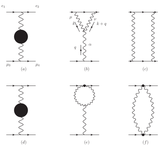
Figure 1: Graphs (a)-(c) are some of the 1-loop contributions to the S-matrx of this four-fermion process. The pinch parts of (b) and (c), shown in (e) and (f) are absorbed into (d), making it become a gauge-invariant effective self-energy.

Although the total $T$ is gauge-independent, the individual components $T_{1}$ $T_{2}$ and $T_{3}$ are gauge dependent. By employing the pinch technique, we recast these into gauge-invariant quantities $\hat{T}_{1}$, $\hat{T}_{2}$, and $\hat{T}_{3}$:

$$T(s,t,m_{e},m_{\mu})=\hat{T}_{1}(t)+\hat{T}_{2}(t,m_{e},m_{\mu})+\hat{T}_{3}(s,t,m_{e},m_{\mu})$$ (67)

From this, we derive the gauge-invariant self-energy $\hat{T}_{1}$.

The PT is a systematic approach. The form of the Ward identity changes depending on the specific physical process. For instance, when a gluon mediates strong interactions, the Ward identity takes the form:

$$k^{\mu}\gamma_{\mu}\equiv\not{k} =(\not{p}+\not{k}-m_{i})-(\not{p}-m_{i})$$ (68)

$$=S^{-1}_{i}(p+k)-S_{i}^{-1}(p)$$

For charged $W^{\pm}$ or neutral $Z$ bosons coupled to fermions, the Ward identity becomes:

$$k^{\mu}\gamma_{\mu}P_{L}\equiv\not{k}P_{L} =(\not{p}+\not{k}-m_{i})P_{L}-P_{R}(\not{p}-m_{j})+m_{i}P_{L}-m_{j}P_{R}$$ (69)

$$=S_{i}^{-1}(p+k)P_{L}-S_{j}^{-1}(p)P_{R}+m_{i}P_{L}-m_{j}P_{R}$$

Here, $P_{R,L}=\frac{1\pm\gamma_{5}}{2}$. The terms $S_{i}^{-1}(p+k)$ and $S_{j}^{-1}(p)$ vanish on shell, leaving behind $m_{i}P_{L}-m_{j}P_{R}$. When charged $W^{\pm}$ couples to fermions, the masses $m_{i}$ and $m_{j}$ differ. For neutral $Z$ fermions of equal mass,$m_{i}=m_{j}$.

Additionally, the vertex in Fig. 1(b) is decomposed into two components:

$$\Gamma_{\mu\nu\alpha}=\Gamma^{P\xi}_{\mu\nu\alpha}+\Gamma^{\xi}_{\mu\nu\alpha},$$ (70)

where

$$\Gamma^{P\xi}_{\mu\nu\alpha}=\frac{1}{\xi}[(q+k)_{\nu}g_{\mu\alpha}+k_{\mu}g_{\nu\alpha}]$$ (71)

$$\Gamma^{\xi}_{\mu\nu\alpha}=2q_{\mu}g_{\nu\alpha}-2q_{\nu}g_{\mu\alpha}-(2k+q)_{\alpha}g_{\mu\nu}+(1-\frac{1}{\xi})[k_{\nu}g_{\mu\alpha}+(k+q)_{\mu}g_{\nu\alpha}],$$

The term $\Gamma^{\xi}_{\mu\nu\alpha}$ satisfies the Ward identity

$$q^{\alpha}\Gamma^{\xi}_{\mu\nu\alpha}=\Delta^{-1}_{\mu\nu}(k,\xi)-\Delta^{-1}_{\mu\nu}(k+q,\xi)$$ (72)

Gauge boson propagators depend on the gauge-fixing parameters:

$$\Delta^{i}_{\mu\nu}(q)=\mathscr{D}^{i}_{\mu\nu}(q)-\frac{q_{\mu}q_{\nu}}{M^{2}_{i}}D^{i}(q)$$ (73)

where

$$D^{i}(q,\xi)=\frac{i}{q^{2}-\xi_{i}M_{i}^{2}}$$

$$\mathscr{D}^{i}_{\mu\nu}(q)=[g_{\mu\nu}-\frac{q_{\mu}q_{\nu}}{M^{2}_{i}}]\frac{-i}{q^{2}-M_{i}^{2}}$$ (74)

$\mathscr{D}^{i}_{\mu\nu}(q)$ are the $W^{\pm}$,$Z$ and $Z^{{}^{\prime}}$ propagators ($\xi\rightarrow\infty$). Selecting the Feynman gauge($\xi=1$) can greatly simplify calculationsPapavassiliou:1994pr . Then, the pinch part of Fig .1(c) vanished. Furthermore, when extracting the Pinch contribution of self energy, the following formula will be used:

$$g^{\alpha}_{\nu}= \Delta^{i}_{\nu\mu}(q,\xi_{i})\Delta^{-1}_{i}(q,\xi_{i})^{\mu\alpha}$$

$$= \Delta^{i}_{\nu\mu}(q,\xi_{i})\mathscr{D}_{i}^{-1}(q)^{\mu\alpha}-iq_{\nu}q^{\alpha}D_{i}(q,\xi)$$

$$q_{\mu}= -i\{q^{2}D_{i}(q,\xi_{i})q_{\mu}+M_{i}^{2}q^{\nu}\Delta^{i}_{\nu\mu}(q,\xi_{i})\}$$ (75)

where

$$\mathscr{D}_{i}^{-1}(q)^{\mu\alpha}=i\{g^{\mu\alpha}(q^{2}-M_{i}^{2})-q^{\mu}q^{\alpha}\}$$ (76)

If $i=\gamma$,

$${\Delta^{\gamma}_{\mu\nu}}^{-1}(q) =iq^{2}[g^{\mu\nu}+(1-\frac{1}{\xi_{\gamma}})\frac{q_{\mu}q_{\nu}}{q^{2}}]$$ (77)

In the B-LSSM, the pinch part of the self-energy of $W^{\pm}$ is similar to the result in the SM, here are the results:

$$\Pi^{P}_{WW}(q^{2})=-4g_{2}^{2}(q^{2}-M_{W}^{2})\{s_{W}^{2}I_{W\gamma}(q^{2})+c_{W}^{2}({c^{\prime}}^{2}I_{WZ}(q^{2})+{s^{\prime}}^{2}I_{WZ}(q^{2}))\}$$ (78)

Where,

$$I_{ij}(q^{2})=i\mu^{4-n}\int\frac{d^{n}k}{(2\pi)^{n}}\frac{1}{(k^{2}-m_{i}^{2})[(k+q)^{2}-m^{2}_{j}]}$$ (79)

The calculation of guage-independent self-energies of $\gamma$,$Z$ and $Z^{{}^{\prime}}$ needs to utilize the following allocation:

$$\frac{g_{2}}{2}\gamma^{\mu}P_{L}=(-i)s_{W}(e\gamma e)^{\mu}-ic_{W}c^{{}^{\prime}}(eZe)^{\mu}+ic_{W}s^{{}^{\prime}}(eZ^{{}^{\prime}}e)^{\mu}$$ (80)

By combining Eq. (75) and Eq. (80), the following results can be obtained:

$$\Pi^{P}_{\gamma\gamma}(q^{2})=-4g_{2}^{2}s_{W}^{2}q^{2}I_{WW}(q^{2})$$

$$\Pi^{P}_{\gamma Z}(q^{2})=-2g_{2}^{2}s_{W}c_{W}c^{{}^{\prime}}(2q^{2}-M_{Z}^{2})I_{WW}(q^{2})$$

$$\Pi^{P}_{\gamma Z^{{}^{\prime}}}(q^{2})=-2g_{2}^{2}s_{W}c_{W}s^{{}^{\prime}}(2q^{2}-M_{Z^{{}^{\prime}}}^{2})I_{WW}(q^{2})$$

$$\Pi^{P}_{ZZ}(q^{2})=-4g_{2}^{2}c^{2}_{W}{c^{{}^{\prime}}}^{2}(q^{2}-M_{Z}^{2})I_{WW}(q^{2})$$

$$\Pi^{P}_{Z^{{}^{\prime}}Z^{{}^{\prime}}}(q^{2})=-4g_{2}^{2}c^{2}_{W}{s^{{}^{\prime}}}^{2}(q^{2}-M_{Z^{{}^{\prime}}}^{2})I_{WW}(q^{2})$$

$$\Pi^{P}_{ZZ^{{}^{\prime}}}(q^{2})=2g_{2}^{2}c^{2}_{W}s^{{}^{\prime}}c^{{}^{\prime}}(2q^{2}-M_{Z}^{2}-M_{Z^{{}^{\prime}}}^{2})I_{WW}(q^{2})$$ (81)

By utilizing PT, we successfully derive gauge-invariant self-energies for the$W^{\pm}$, $Z$, $Z^{\prime}$ and $\gamma$ bosons, which are essential for subsequent calculations.bosons, which are essential for subsequent calculations.

IV Formalism of Oblique Corrections

IV.1 Formalism of S T U paramaters in the B-LSSM

The implementation of renormalization schemes that utilize the number of observables equivalent to the number of free parameters may prove challenging in practice. This is due to the necessity of solving a more extensive set of equations than those encountered in the SM, which may result in the generation of highly intricate and unwieldy analytical formulae Chankowski:2006jk .

The oblique parameters are the products of renormalization under the SM, and thus warrant examination to ascertain whether such a quantity remains well-defined in the B-LSSM. A significant indicator is whether the divergence of oblique parameters is cancelled. From a technical standpoint, it appears that the requisite divergent elimination is guaranteed by the symmetry of the group, since $Tr[T^{3}Y]=0$.

	$Q$	$L$	$H_{d}$	$H_{u}$	$d$	$u$	$e$	$\nu$	$\eta$	$\bar{\eta}$
$Y$	$\frac{1}{6}$	$-\frac{1}{2}$	$-\frac{1}{2}$	$\frac{1}{2}$	$\frac{1}{3}$	$\frac{2}{3}$	-1	0	0	0
$T^{3}$	$\frac{1}{2}$ 0 0 $-\frac{1}{2}$	$\frac{1}{2}$ 0 0 $-\frac{1}{2}$	$\frac{1}{2}$ 0 0 $-\frac{1}{2}$	$\frac{1}{2}$ 0 0 $-\frac{1}{2}$	0	0	0	0	0	0
$Y_{B}$	$\frac{1}{6}$	$-\frac{1}{2}$	0	0	$-\frac{1}{6}$	$-\frac{1}{6}$	$\frac{1}{2}$	$\frac{1}{2}$	-1	1
$T^{3}\times Y$	$\frac{1}{12}$ 0 0 $-\frac{1}{12}$	$-\frac{1}{2}$ 0 0 $\frac{1}{2}$	$-\frac{1}{2}$ 0 0 $\frac{1}{2}$	$\frac{1}{2}$ 0 0 $-\frac{1}{2}$	0	0	0	0	0	0
$T^{3}\times Y_{B}$	$\frac{1}{12}$ 0 0 $-\frac{1}{12}$	$-\frac{1}{2}$ 0 0 $\frac{1}{2}$	0	0	0	0	0	0	0	0
$Y\times Y_{B}$	$\frac{1}{36}$	$\frac{1}{4}$	0	0	$\frac{1}{18}$	$-\frac{1}{9}$	$-\frac{1}{2}$	0	0	0

Table 1: The charges and the mixed products of each superfield in the B-LSSM

As can be observed in the Tab. 1, the self-energy functions, namely, the unrenormalized vacuum polarisation functions with coupling constants factored out, namely, the ($\Pi^{\prime}s$), will cancel out any divergence after traversing all the superfields. It is therefore reasonable to continue using the original definition of Peskin Peskin:1991sw :

$$\alpha S\equiv 4e^{2}[\Pi^{\prime}_{33}(0)-\Pi^{\prime}_{3Q}(0)]$$

$$\alpha T\equiv \frac{e^{2}}{s_{W}^{2}c_{W}^{2}\widetilde{m_{Z}}^{2}}[\Pi_{11}(0)-\Pi_{33}(0)]$$ (82)

$$\alpha U\equiv 4e^{2}[\Pi^{\prime}_{11}(0)-\Pi^{\prime}_{31}(0)]$$

where $\widetilde{m_{Z}}^{2}={c^{\prime}}^{2}m_{Z}^{2}+{s^{\prime}}^{2}m_{Z^{\prime}}^{2}$.

In accordance with Peskin’s approach, the one-particle-irreducible (1PI) self-energies of the photon, $Z$ and $Z^{\prime}$ in the B-LSSM are expressed as a linear combination of the $T_{3}-Q-B$-mixed eigenstate self-energy.

$$\Pi_{AA}=e^{2}\Pi_{QQ}$$ (83a)

$$\Pi_{ZA}=\frac{e^{2}c^{\prime}}{s_{W}c_{W}}(\Pi_{3Q}-s_{W}^{2}\Pi_{QQ})+es^{\prime}g_{E}\Pi_{QB}$$ (83b)

$$\Pi_{Z^{{}^{\prime}}A}=-\frac{e^{2}s^{\prime}}{s_{W}c_{W}}(\Pi_{3Q}-s_{W}^{2}\Pi_{QQ})+ec^{\prime}g_{E}\Pi_{QB}$$ (83c)

$$\Pi_{ZZ}=\frac{e^{2}{c^{\prime}}^{2}}{s_{W}^{2}c_{W}^{2}}(\Pi_{33}-2s_{W}^{2}\Pi_{3Q}+s_{W}^{4}\Pi_{QQ})$$

$$\qquad\quad\;+2\frac{es^{\prime}c^{\prime}}{s_{W}c_{W}}g_{E}(\Pi_{3B}-s^{2}_{W}\Pi_{QB})+{s^{\prime}}^{2}g^{2}_{E}\Pi_{BB}$$ (83d)

$$\Pi_{Z^{{}^{\prime}}Z^{{}^{\prime}}}=\frac{e^{2}{s^{\prime}}^{2}}{s_{W}^{2}c_{W}^{2}}(\Pi_{33}-2s_{W}^{2}\Pi_{3Q}+s_{W}^{4}\Pi_{QQ})$$

$$\qquad\quad\;-2\frac{es^{\prime}c^{\prime}}{s_{W}c_{W}}g_{E}(\Pi_{3B}-s^{2}_{W}\Pi_{QB})+{c^{\prime}}^{2}g^{2}_{E}\Pi_{BB}$$ (83e)

$$\Pi_{ZZ^{{}^{\prime}}}=-\frac{e^{2}c^{\prime}s^{\prime}}{s_{W}^{2}c_{W}^{2}}(\Pi_{33}-2s_{W}^{2}\Pi_{3Q}+s_{W}^{4}\Pi_{QQ})$$

$$\qquad\quad\;+2\frac{e({c^{\prime}}^{2}-{s^{\prime}}^{2})}{s_{W}c_{W}}g_{E}(\Pi_{3B}-s^{2}_{W}\Pi_{QB})+c^{\prime}s^{\prime}g^{2}_{E}\Pi_{BB}$$ (83f)

Where $g_{E}=g_{B}+\frac{Y}{Y_{B}}g_{YB}$, $Q$ indicates the charge of photon, $T_{3}$ indicates the charge of $W_{3}$ and $B$ indicates the charge of $U(1)_{B-L}$ group. The 1PI self energy of $W^{\pm}$ is given as:

$$\Pi_{WW}=\frac{e^{2}}{s_{W}^{2}}\Pi_{11}$$ (84)

We can linearly combine the above equations and define effective self-energy $\widetilde{\Pi}_{ZA}$ and $\widetilde{\Pi}_{ZZ}$ as follows to eliminate the self-energys ”containing” $U_{1}$ charge $B$: $\widetilde{\Pi}_{ZA}=c^{\prime}(\ref{pi2})-s^{\prime}(\ref{pi3})$, $\widetilde{\Pi}_{ZZ}={c^{\prime}}^{2}(\ref{pi4})-2c^{\prime}s^{\prime}(\ref{pi6})+{s^{\prime}}^{2}(\ref{pi5})$. Combining with (83a), one can obtain:

$$\Pi_{AA}=e^{2}\Pi_{QQ}$$ (85a)

$$\widetilde{\Pi}_{ZA}=\frac{e^{2}}{s_{W}c_{W}}(\Pi_{3Q}-s_{W}^{2}\Pi_{QQ})$$ (85b)

$$\widetilde{\Pi}_{ZZ}=\frac{e^{2}}{s_{W}^{2}c_{W}^{2}}(\Pi_{33}-2s_{W}^{2}\Pi_{3Q}+s_{W}^{4}\Pi_{QQ})$$ (85c)

Combining the definition of oblique parameters Eq. (82), Eq. (84) and Eq. (85), one can obtain the expression of oblique parameters under the B-LSSM:

$$\alpha S= 4s_{W}c_{W}[\widetilde{\Pi}^{\prime}_{ZZ}(0)-\frac{c_{W}^{2}-s_{W}^{2}}{s_{W}c_{W}}\widetilde{\Pi}^{\prime}_{Z\gamma}(0)-\Pi^{\prime}_{\gamma\gamma}(0)]$$

$$\alpha T= \frac{\Pi_{WW}(0)}{m^{2}_{W}}-\frac{\widetilde{\Pi}_{ZZ}(0)+\frac{2s_{W}}{c_{W}}\widetilde{\Pi}_{Z\gamma}(0)+\frac{s^{2}_{W}}{c_{W}^{2}}\Pi^{\prime}_{\gamma\gamma}(0)}{m^{2}_{Z}}$$ (86)

$$\alpha U= 4s_{W}^{2}[\Pi^{\prime}_{WW}(0)-c_{W}^{2}\widetilde{\Pi}^{\prime}_{ZZ}(0)-2s_{w}c_{W}\widetilde{\Pi}^{\prime}_{Z\gamma}(0)-s_{W}^{2}\Pi^{\prime}_{\gamma\gamma}(0)]$$

IV.2 The S T U paramaters in the effective-Lagrangian

For the case of $Z$ couples with two fermions, neutral-current of $Z$ particle can be expressed as follows:

$$J_{Z}^{\mu}= [\frac{e}{s_{W}c_{W}}(T^{3}-s^{2}Q)c^{{}^{\prime}}+g_{E}Y_{B}s^{{}^{\prime}}]\bar{\psi}\gamma^{\mu}P_{L}\psi$$

$$+[\frac{e}{s_{W}c_{W}}(-s_{W}^{2}Q)c^{{}^{\prime}}+g_{E}Y_{B}s^{{}^{\prime}}]\bar{\psi}\gamma^{\mu}P_{R}\psi$$

Using Eq. (62) and $g_{E}=g_{B}+\frac{Y}{Y_{B}}g_{YB}$, The neutral-current coupling between the Z boson and SM leptons in the B-LSSM can be written as follows:

$$\mathcal{L}_{N,Zff}= G(c^{\prime}-s^{\prime}\frac{c^{\prime}s^{\prime}(m^{2}_{Z}-m^{2}_{Z^{\prime}})}{{c^{\prime}}^{2}m^{2}_{Z}+{s^{\prime}}^{2}m^{2}_{Z^{\prime}}})$$

$$\times Z^{\mu}\bar{f}\gamma_{\mu}[T^{3}P_{L}-(s_{W}^{2}-\frac{s^{\prime}(c^{2}_{W}c^{\prime}s^{\prime}(m^{2}_{Z}-m^{2}_{Z^{\prime}})+\frac{xm_{Z}m_{Z^{\prime}}}{2})}{{c^{\prime}}^{2}m^{2}_{Z}+{s^{\prime}}^{2}m^{2}_{Z^{\prime}}})]f$$ (88)

Using the effective-Lagrangian techniques given by Burgess:1993vc

$$\mathcal{L}_{N,Zee}= \frac{e}{\hat{s_{W}}\hat{c_{W}}}(1+\frac{\alpha T}{2})Z^{\mu}\bar{f}\gamma_{\mu}[T^{3}P_{L}-(\hat{s_{W}}^{2}+\frac{\alpha S}{4(\hat{c_{W}}^{2}-\hat{s_{W}}^{2})}-\frac{\hat{c_{W}}^{2}\hat{s_{W}}^{2}\alpha T}{\hat{c_{W}}^{2}-\hat{s_{W}}^{2}})]f$$

$$\mathcal{L}_{C,We\nu}= -\frac{e}{\sqrt{2}\hat{s_{W}}}(1-\frac{\alpha S}{4(\hat{c_{W}}^{2}-\hat{s_{W}}^{2})}+\frac{\hat{c_{W}}^{2}\alpha T}{2(\hat{c_{W}}^{2}-\hat{s_{W}}^{2})}+\frac{\alpha U}{8\hat{s}^{2}}){W^{\pm}}^{\mu}\bar{f}\gamma_{\mu}P_{L}f$$ (89)

Where $\hat{s_{W}}$ and $\hat{c_{W}}$ are defined by

$$\hat{s_{W}}\hat{c_{W}}m_{Z}=\frac{1}{2}ev=s_{W}c_{W}m_{Z}^{SM}$$ (90)

Comparing Eq. (88) and Eq. (89), one can obtain:

$$\alpha T= 2[\frac{\hat{s_{W}}\hat{c_{W}}}{s_{W}c_{W}}(c^{\prime}-s^{\prime}\frac{c^{\prime}s^{\prime}(m^{2}_{Z^{\prime}}-m^{2}_{Z})}{{c^{\prime}}^{2}m_{Z}^{2}+{s^{\prime}}^{2}m_{Z^{\prime}}^{2}})-1]$$

$$\alpha S= 4\hat{c_{W}}^{2}\hat{s_{W}}^{2}\alpha T+4(\hat{c_{W}}^{2}-\hat{s_{W}}^{2})(s_{W}^{2}-\hat{s_{W}}^{2}-\frac{s^{\prime}}{c^{\prime}}\frac{c_{W}^{2}c^{\prime}s^{\prime}(m^{2}_{Z^{\prime}}-m^{2}_{Z})+\frac{xm_{Z}m_{Z^{\prime}}}{2}}{{c^{\prime}}^{2}m^{2}_{Z}+{s^{\prime}}^{2}m_{Z^{\prime}}^{2}})$$

$$\alpha U= 8\hat{s_{W}}^{2}(\frac{\hat{s_{W}}}{s_{W}}-1+\frac{\alpha S}{4(\hat{c_{W}}^{2}-\hat{s_{W}}^{2})}-\frac{\hat{c_{W}}^{2}\alpha T}{2(\hat{c_{W}}^{2}-\hat{s_{W}}^{2})})$$ (91)

It can be demonstrated that the definition of $\hat{c_{W}}$ is indeed equivalent to the the Sirlin definition Sirlin:1980nh , based on the values of $m_{W}$ and $m_{Z}$. In comparison to the intrinsic definition of $c_{W}$ at the tree level, these can be connected by means of the equation:

$$\Delta s=\hat{s_{W}}-s_{W}$$

$$\hat{c_{W}}^{2}=\frac{m_{W}^{2}}{m_{Z}^{2}}$$

$$c^{2}_{W}=\frac{m^{2}_{W}}{{c^{\prime}}^{2}m_{Z}+{s^{\prime}}^{2}m_{Z^{\prime}}^{2}}=1-s_{W}^{2}$$

$$\qquad\!\!=1-\hat{s_{W}}^{2}+2\hat{s_{W}}\Delta s=\hat{c_{W}}^{2}+2\hat{s_{W}}\Delta s$$ (92)

By comparing the three equations in Eq. (92), one can obtain:

$${s^{\prime}}^{2}(\frac{m^{2}_{Z^{\prime}}}{m^{2}_{Z}}-1)=-2\frac{\hat{s_{W}}}{\hat{c_{W}}^{2}}\Delta s$$ (93)

Combining Eq. (91) and Eq. (93), one can obtain the following results through small-scale analysis:

$$\alpha T= 2\frac{\Delta s}{\hat{s_{W}}}-{s^{\prime}}^{2}$$ (94)

$$\alpha S+\alpha U= 8\hat{s_{W}}\Delta s-4s^{\prime}\frac{\hat{c_{W}}\hat{s_{W}}}{e}g_{B}$$ (95)

$$2\hat{s_{W}}^{2}\alpha S+(\hat{s_{W}}^{2}-\hat{c_{W}}^{2})\alpha U= 4\hat{c_{W}}^{2}\hat{s_{W}}^{2}\alpha T+8\hat{s_{W}}(\hat{s_{W}}^{2}-\hat{c_{W}}^{2})\Delta s$$ (96)

The aforementioned formulas are conducive to the analysis of relationship between $s^{\prime}$, $\Delta s$ and $g_{B}$.

IV.3 Gauge-invariant electroweak interaction parameters

We have already provided the pinch contributions of all self energy-graphs of gauge particles in Eq. (78) and Eq. (81), and also provided specific expressions for the $S$ $T$ $U$ parameters in (85) and Eq. (86). Combining the above four equations, we can obtain pinch parts of the $S$ $T$ $U$ paramaters. The gauge-invariant $S$ $T$ $U$ parameters can be represented as the sum of the pinch parts and the conventional parts:

$$\alpha(S)_{GI}= \alpha(S)_{C}+8g^{2}_{2}s_{W}c_{W}I^{\prime}_{WW}(0)({c^{\prime}}^{2}m_{Z}^{2}+{s^{\prime}}^{2}m_{Z^{\prime}}^{2})$$ (97)

$$\alpha(T)_{GI}= \alpha(T)_{C}+4g^{2}_{2}[s_{W}^{2}I_{W\gamma}(0)+c_{W}^{2}({c^{\prime}}^{2}I_{WZ}(0)+{s^{\prime}}^{2}I_{WZ^{\prime}}(0))-I_{WW}(0)]$$ (98)

$$\alpha(U)_{GI}= \alpha(U)_{C}+16s_{W}^{2}g^{2}_{2}\{m^{2}_{W}[s_{W}^{2}I^{\prime}_{W\gamma}(0)+c_{W}^{2}({c^{\prime}}^{2}I^{\prime}_{WZ}(0)+{s^{\prime}}^{2}I^{\prime}_{WZ^{\prime}}(0))$$

$$-I^{\prime}_{WW}(0)]-[s_{W}^{2}I_{W\gamma}(0)+c_{W}^{2}({c^{\prime}}^{2}I_{WZ}(0)+{s^{\prime}}^{2}I_{WZ^{\prime}}(0))-I_{WW}(0)]\}$$ (99)

Formally speaking, our results are extensions of Degrassi’s results Degrassi:1993kn based on the SM. The divergence of both has been cancel out, This proves the viewpoint of the first subsection of this section.

V The divergence cancellation of S T U parameters in the Neutralino-Chargino sector and srquark sector

In the context of one-loop diagram calculations, particularly in the context of shell renormalization, the elimination of divergences serves as a crucial indicator for the verification of calculation results. This chapter presents the divergence cancellation of $S$, $T$ and $U$ parameters in the neutralino-chargino sector and squark sector, with the objective of further validating the theoretical framework.

V.1 Neutralino-Chargino sector

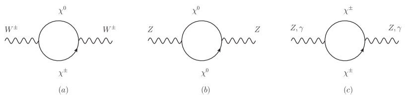
Figure 2: Vacuum polarization diagram with Neutralino-Chargino sector

The calculation of the vacuum polarization diagrams of fermions as loop particles is presented in Appendix B, along with a processing of all the coefficients involved. As a consequence of the non-divergence of the derivative of the $B_{0}$ function, the divergence of the $S$ and $U$ parameters is directly proportional to $\mathcal{C}_{1}$. By combining equations Eq. (85) and Appendix B, the divergences of the $S$ $T$ and $U$ parameters ($div_{S}$, $div_{T}$ and $div_{U}$) can be expressed as:

$$div_{S}\sim -\frac{G^{2}}{4}[-\sum_{i,j}^{2}(U^{*}_{j2}U_{i2}U^{*}_{i2}U_{j2}+V^{*}_{j2}V_{i2}V^{*}_{i2}V_{j2})+\sum_{i,j}^{7}(N^{*}_{j3}N_{i3}-N^{*}_{j4}N_{i4})^{2}]=0$$

$$div_{U}\sim -\frac{c_{W}^{2}G^{2}}{4}\{\sum_{i,j}^{7,2}[4U^{*}_{j1}N_{i2}N^{*}_{i2}U_{j1}+2U^{*}_{j2}N_{i3}N^{*}_{i3}U_{j2}+2\sqrt{2}(U^{*}_{j1}N_{i2}N^{*}_{i3}U_{j1}+h.c.)$$

$$+4V^{*}_{j1}N_{i2}N^{*}_{i2}V_{j1}+2V^{*}_{j2}N_{i4}N^{*}_{i4}V_{j2}-2\sqrt{2}(V^{*}_{j1}N_{i2}N^{*}_{i4}V_{j2}+h.c.)]$$

$$-\sum_{i,j}^{2}[4U^{*}_{j1}U_{i1}U_{i1}U^{*}_{j1}+4V^{*}_{j1}V_{i1}V_{i1}V^{*}_{j1}+U^{*}_{j2}U_{i2}U_{i2}U^{*}_{j2}+V^{*}_{j1}V_{i1}V_{i2}V^{*}_{j2}$$

$$+2c_{W}^{2}(U^{*}_{j1}U_{i1}U^{*}_{i2}U_{j2}+V^{*}_{j1}V_{i1}V^{*}_{i2}V_{j2})+2(1+2s_{W}^{2})(U^{*}_{j2}U_{i2}U^{*}_{i1}U_{j1}+V^{*}_{j2}V_{i2}V^{*}_{i1}V_{j1})]$$

$$-\sum_{i,j}^{7}(N^{*}_{j3}N_{i3}-N^{*}_{j4}N_{i4})^{2}\}=0$$

$$div_{T}\sim -\frac{G^{2}}{4m_{Z}^{2}}\{\mathcal{A}_{1}-\mathcal{A}_{2}\}$$

Where,

$$\mathcal{A}_{1}= \sum_{i,j}^{2,7}(m_{\chi_{i}^{\pm}}^{2}+m_{\chi_{j}^{0}}^{2})[4U^{*}_{j1}N_{i2}N^{*}_{i2}U_{j1}+2U^{*}_{j2}N_{i3}N^{*}_{i3}U_{j2}+2\sqrt{2}(U^{*}_{j1}N_{i2}N^{*}_{i3}U_{j1}+h.c.)$$

$$+4V^{*}_{j1}N_{i2}N^{*}_{i2}V_{j1}+2V^{*}_{j2}N_{i4}N^{*}_{i4}V_{j2}-2\sqrt{2}(V^{*}_{j1}N_{i2}N^{*}_{i4}V_{j2}+h.c.)]$$

$$-\sum_{i,j}^{2}(m_{\chi_{i}^{\pm}}^{2}+m_{\chi_{j}^{\pm}}^{2})[4c_{W}^{4}U^{*}_{j1}U_{i1}U^{*}_{i1}U_{j1}+c_{2W}^{2}U^{*}_{j2}U_{i2}U^{*}_{i2}U_{j2}+2c_{W}^{2}c_{2W}(U^{*}_{j1}U_{i1}U^{*}_{i2}U_{j2}+h.c.)$$

$$+4c_{W}^{4}V^{*}_{j1}V_{i1}V^{*}_{i1}V_{j1}+c_{2W}^{2}2V^{*}_{j2}V_{i2}V^{*}_{i2}V_{j2}+2c_{W}^{2}c_{2W}(V^{*}_{j1}V_{i1}V^{*}_{i2}V_{j2}+h.c.)]$$

$$-\sum_{i,j}^{7}(m_{\chi_{i}^{0}}^{2}+m_{\chi_{j}^{0}}^{2})(N^{*}_{j3}N_{i3}-N^{*}_{j4}N_{i4})^{2}$$

$$\mathcal{A}_{2}= \sum_{i,j}^{2,7}2m_{\chi_{i}^{\pm}}m_{\chi_{j}^{0}}[4U^{*}_{j1}N_{i2}V^{*}_{j1}N_{i2}-2U^{*}_{j2}N_{i3}V^{*}_{j2}N_{i4}-2\sqrt{2}U^{*}_{j1}N_{i2}V^{*}_{j2}N^{*}_{j4}+2\sqrt{2}U^{*}_{j2}N_{i3}V_{i1}N^{*}_{j2}$$

$$+4N^{*}_{j2}U_{1}N^{*}_{j2}V_{i1}+2N^{*}_{j3}U_{i2}N^{*}_{j4}V_{i2}-2\sqrt{2}N^{*}_{j2}U_{i1}N^{*}_{j4}V_{i2}+2\sqrt{2}N^{*}_{j3}U_{i2}N^{*}_{j2}V_{i1}]$$

$$-\sum_{i,j}^{2}2m_{\chi_{i}^{\pm}}m_{\chi_{j}^{\pm}}[4c_{W}^{4}U^{*}_{j1}U_{i1}V_{j1}V^{*}_{i1}+c_{2W}^{2}U^{*}_{j2}U_{i2}V_{j2}V^{*}_{i2}+2c_{W}^{2}c_{2W}(U^{*}_{j1}U_{i1}V_{j2}V^{*}_{i2}+h.c.)$$

$$+4c_{W}^{4}V^{*}_{j1}V_{i1}U_{j1}U^{*}_{i2}+c_{2W}^{2}V^{*}_{j2}V_{i2}U_{j2}U^{*}_{i2}+2c_{W}^{2}c_{2W}(V^{*}_{j1}V_{i1}U_{j2}U^{*}_{i2}+h.c.)]$$

$$-\sum_{i,j}^{7}2m_{\chi_{i}^{0}}m_{\chi_{j}^{0}}(N^{*}_{j3}N_{i3}-N^{*}_{j4}N_{i4})^{2}$$

Using the corresponding mass matrix diagonalization formula:

$$\sum_{i}^{2}U^{*}_{ik}m_{\chi^{\pm}_{i}}V_{ij}V^{*}_{ij}m_{\chi^{\pm}_{i}}U_{ik}=\sum_{j}^{2}(M_{\chi^{\pm}})^{2}_{kj}$$

$$\sum_{ij}^{2}U^{*}_{ik}U_{jk}V^{*}_{jl}V^{*}_{il}m_{\chi_{i}^{\pm}}m_{\chi_{j}^{\pm}}=(M_{\chi^{\pm}})^{2}_{kl}$$ (100)

one can obtain:

$$\mathcal{A}_{1}= 16M_{2}^{2}+g_{2}^{2}v^{2}+2\mu^{2}+2g_{2}^{2}v^{2}+\frac{1}{2}g_{YB}v^{2}-4c_{W}^{4}(4M_{2}^{2}+g_{2}^{2}v^{2})$$

$$+c_{2W}^{2}(4\mu^{2}+g_{2}^{2}v^{2})-(2\mu^{2}+2g_{2}^{2}v^{2}+\frac{1}{2}g_{YB}v^{2})$$

$$= (16c_{W}^{4}-16)M_{2}^{2}+(4c_{2W}^{2}-4)\mu^{2}+(4c_{W}^{4}+c_{2W}^{2}-5)g_{2}^{2}v^{2}$$

$$\mathcal{A}_{2}= 2\times[8M^{2}_{2}+4\mu^{2}+g_{2}^{2}v^{2}-(8c_{W}^{4}M_{2}^{2}+2c_{2W}^{2}\mu^{2}+2c_{W}^{2}c_{2W}{g_{2}^{2}v^{2}})+2\mu^{2}]$$

$$= (16c_{W}^{4}-16)M_{2}^{2}+(4c_{2W}^{2}-4)\mu^{2}+(4c_{W}^{4}+c_{2W}^{2}-5)g_{2}^{2}v^{2}$$

It can be seen from this that their divergence cancels out each other !

V.2 Squark sector

When superquarks are loop particles in the one-loop self-energy diagrams, the cancellation of divergences in the $S$, $T$, and $U$ parameters can be demonstrated as follows.

$$div_{S}\sim -\frac{4}{3\alpha}s_{W}c_{W}[\mathcal{C}_{a}^{\gamma\gamma}-\frac{c_{W}^{2}-s_{W}^{2}}{s_{W}c_{W}}\widetilde{\mathcal{C}}_{a}^{Z\gamma}-\widetilde{\mathcal{C}}_{a}^{ZZ}]$$

$$= \frac{4}{\alpha}s_{W}c_{W}[(\sum^{3}_{k=1}Z^{U*}_{ik}Z^{U}_{ik})^{2}+4(\sum^{6}_{k=4}Z^{U*}_{ik}Z^{U}_{ik})^{2}-(\sum^{3}_{k=1}Z^{D*}_{ik}Z^{D}_{ik})^{2}+2(\sum^{6}_{k=4}Z^{D*}_{ik}Z^{D}_{ik})^{2}]$$

$$= 0$$

$$div_{U}\sim \frac{4}{\alpha}s_{W}^{2}[\mathcal{C}_{a}^{WW}-s_{W}^{2}\mathcal{C}_{a}^{\gamma\gamma}-2s_{W}c_{W}\widetilde{\mathcal{C}}_{a}^{Z\gamma}-c_{W}^{2}\widetilde{\mathcal{C}}_{a}^{ZZ}]$$

$$= \frac{4}{\alpha}s_{W}^{2}[-\frac{1}{2}g^{2}_{2}\sum^{3}_{k=1}(Z^{D*}_{jk}Z^{U}_{ik})\sum^{3}_{l=1}(Z^{U*}_{il}Z^{D}_{jl})+\frac{1}{4}g^{2}_{2}(\sum^{3}_{k=1}Z^{U*}_{ik}Z^{U}_{ik})^{2}+\frac{1}{4}g^{2}_{2}(\sum^{3}_{k=1}Z^{D*}_{ik}Z^{D}_{ik})^{2}]$$

$$= 0$$

$$div_{T}\sim \frac{1}{m^{2}_{W}}[\sum^{6}_{i,j}\mathcal{C}_{a}^{WW}(m^{2}_{\widetilde{U}_{i}}+m^{2}_{\widetilde{D}_{j}})+\sum^{6}_{i}\mathcal{C}_{b}^{WWU}m^{2}_{\widetilde{U}_{i}}+\sum^{6}_{j}\mathcal{C}_{b}^{WWD}m^{2}_{\widetilde{D}_{j}}]$$

$$-\frac{1}{{c^{\prime}}^{2}m^{2}_{Z}+{s^{\prime}}^{2}m^{2}_{Z^{\prime}}}[\sum^{6}_{i}\widetilde{\mathcal{C}}_{a}^{ZZU}m^{2}_{\widetilde{U}_{i}}+\sum^{6}_{j}\widetilde{\mathcal{C}}_{a}^{ZZD}m^{2}_{\widetilde{D}_{j}}+\frac{1}{2}\sum^{6}_{i}\widetilde{\mathcal{C}}_{b}^{ZZU}m^{2}_{\widetilde{U}_{i}}+\frac{1}{2}\sum^{6}_{j}\widetilde{\mathcal{C}}_{b}^{ZZD}m^{2}_{\widetilde{D}_{j}}$$

$$+\frac{s_{W}}{2c_{W}}(\sum^{6}_{i}\widetilde{\mathcal{C}}_{a}^{Z\gamma U}m^{2}_{\widetilde{U}_{i}}+\sum^{6}_{j}\widetilde{\mathcal{C}}_{a}^{Z\gamma D}m^{2}_{\widetilde{D}_{j}}+\frac{1}{2}\sum^{6}_{i}\widetilde{\mathcal{C}}_{b}^{Z\gamma U}m^{2}_{\widetilde{U}_{i}}+\frac{1}{2}\sum^{6}_{j}\widetilde{\mathcal{C}}_{b}^{Z\gamma D}m^{2}_{\widetilde{D}_{j}})]$$

$$= \frac{0}{m^{2}_{W}}-\frac{0}{{c^{\prime}}^{2}m^{2}_{Z}+{s^{\prime}}^{2}m^{2}_{Z^{\prime}}}$$

$$= 0$$

The specific coefficients for this process have been placed in Appendix A. In the demonstration above, we utilized the unitarity relation of the transposed matrix:

$$\sum^{6}_{k=1}(Z^{U}_{ik}Z^{U*}_{jk})=\sum^{6}_{k=1}(Z^{D}_{ik}Z^{D*}_{jk})=\delta_{ij}$$

VI numerical analysis

A study provided the global fitting of $S$ $T$ and $U$ parameters with recently measured top quark mass data from CMS laboratorydeBlas:2022hdk :

$$S=0.005\pm 0.096\qquad T=0.04\pm 0.12\qquad U=0.134\pm 0.087$$

$$\rho_{ST}=0.91\qquad\quad\qquad \rho_{SU}=-0.65\quad\qquad\rho_{TU}=-0.88$$

In order to study how the parameters affect the vaules of the $S$, $T$ and $U$ parameters, we use the Mathematica to calculate the oblique parameters of the B-LSSM. Some parmeters we assumed are: $A_{t}=3~\rm TeV$, $A_{b}=3~\rm TeV$, $g_{YB}=-0.3$, $g_{B}=0.5$, $\tan\beta=20$, $\tan\beta^{\prime}=1.5$, $m_{Z^{\prime}}=4500~\rm GeV$, $\mu=200~\rm GeV$, $\mu_{B}=800~\rm GeV$, $m_{B}=600~\rm GeV$, $m_{BL}=800~\rm GeV$ $m_{1}=200~\rm GeV$ and $m_{2}=300~\rm GeV$. We use this set of data as a benchmark and run some of the variables respectively. By filtering, we can obtain some parameters that are sensitive to $S$, $T$ and $U$ parameters

Figure 3: S and T parameters that are more sensitive to $m_{1}$, $m_{2}$, and $\mu$.

When we run $m_{1}$, $m_{2}$ and $\mu$ in the $(200~\rm GeV\sim 2000~\rm GeV)$, $(200~\rm GeV\sim 800~\rm GeV)$ and $(200~\rm GeV\sim 800~\rm GeV)$ intervals respectively, we find that they are sensitive to the $S$ and $T$ parameters. The Fig. 3 shows that the $S$ parameter gradually decreases with the increase of $m_{1}$, $m_{2}$, and $\mu$, while the $T$ parameter shows an upward trend with the increase of $m_{1}$ and $m_{2}$. $m_{1}$ and $m_{2}$ are the diagonal elements in the mass matrices of neutralinos and charginos, and their increase weakens the mixing of the matrices, which is the source of the contributions of oblique parameters. $m_{2}$ is the diagonal element with the highest value in the mass matrices of neutralinos and charginos, which explains its sensitivity to oblique parameters relative to $m_{1}$.

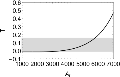
Figure 4: T and U parameters that are more sensitive to $A_{t}$.

Fig. 4 illustrates the changes in the $T$ and $U$ parameters as the $A_{t}$ parameter varies from $1000~\rm GeV$ to $7000~\rm GeV$. The gray area indicates one standard deviation of the experimental observations. As shown, the $T$ parameter increases with the rise in $A_{t}$, while the $U$ parameter exhibits the opposite trend. The observed changes in the $T$ and $U$ parameters in Fig. 4 are primarily due to the contributions from the Feynman diagrams involving squark fields as loop particles. The $A_{t}$ parameter, originating from the off-diagonal elements of the squark mass matrix, influences the mixing between the left-handed and right-handed $\widetilde{u}$ squarks ($\widetilde{u}_{L}$ and $\widetilde{u}_{R}$), which in turn drives the squark sector’s contributions to the oblique parameters.

We performed a random three-dimensional sampling of the $S$, $T$, and $U$ parameters in Eq. (94-96) based on the probability distribution results obtained from the experimental fits. Each randomly selected point corresponds to a unique set of values for $\Delta s$, $s^{\prime 2}$, and $g_{B}$. We then conducted statistical analysis on the resulting $\Delta s$, $s^{\prime 2}$, and $g_{B}$ values to generate probability histograms. As shown in Fig. 5, the distribution of $\Delta s$ does not exceed one standard deviation of the current experimental measurements, making it challenging to extract further useful information from the measurement of the Weinberg angle. Additionally, the probability distribution of $g_{B}$ exhibits a sharp peak around $g_{B}=0.09$, with a rapid decay for $g_{B}>0.2$. Analysis reveals that the probability for $0.03<g_{B}<0.21$ exceeds ninety percent when compared to the entire range.

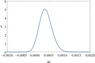
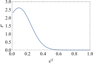
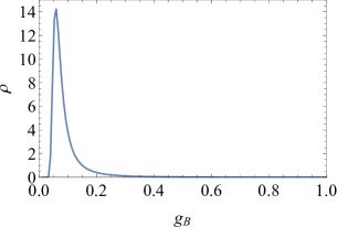
Figure 5: By using the Monte Carlo sampling method and generating statistical histograms, the probability distributions of the three parameters can be obtained.

VII Conclusions

Using the pinch technique, we derive the gauge-invariant self-energy of gauge bosons in the B-LSSM and obtain gauge-invariant oblique parameters. This approach ensures gauge symmetry when extracting information from S-matrix elements.

In models featuring an additional $U(1)$ symmetry compare to the Standard Model, the definitions of oblique parameters remain applicable. From the perspective of divergence cancellation, these definitions are comprehensive and can be extended to the models, which include various types of group expansion, thereby simplifying the complex definitions and proofs associated with the $S$, $T$, and $U$ parameters.

In this work, the contributions to the $S$, $T$, and $U$ parameters from two key sectors of the B-LSSM are calculated and the impacts of model parameters in the B-LSSM are analyzed. The parameter space of the B-LSSM we selected aligns well with the global fitting of the $S$, $T$, and $U$ parameters reported in the experiments.

Using the effective Lagrangian and experimental measurements, the coupling constant of the $U(1)$ group in models with an additional $U(1)$ symmetry can be related to the $S$, $T$, and $U$ parameters. Through analysis, effective constraints on these coefficients can be derived.

By comparing the effective Lagrangian with the model’s Lagrangian and combining the results from fitting experimental measurements, the coupling constant of the $U(1)$ group in models with an additional $U(1)$ symmetry can be related to the $S$, $T$, and $U$ parameters. Through analysis, effective constraints on these coefficients can be imposed.

Appendix A Integral formulas for some Feynman diagrams

Here we provide some integral formulas for vacuum polarization diagrams, we will unify them here in the form of $A$ or $B$ functions. We define $A$ fuctions:

$$i\pi^{2}A_{0}(m)= \mu^{4-n}\int d^{n}q\frac{1}{q^{2}+m^{2}-i\epsilon}$$

$$i\pi^{2}A_{\mu}(m)= \mu^{4-n}\int d^{n}q\frac{q_{\mu}}{q^{2}+m^{2}-i\epsilon}=0$$

$$i\pi^{2}A_{\mu\nu}(m)= \mu^{4-n}\int d^{n}q\frac{q_{\mu}q_{\nu}}{q^{2}+m^{2}-i\epsilon}=i\pi^{2}A_{2}(m)g_{\mu\nu}$$ (101)

and $B$ fuctions:

$$i\pi^{2}B_{0}(p^{2};m_{1},m_{2})= \mu^{4-n}\int d^{n}q\frac{1}{d_{0}d_{1}}$$

$$i\pi^{2}B_{\mu}(p^{2};m_{1},m_{2})= \mu^{4-n}\int d^{n}q\frac{q_{\mu}}{d_{0}d_{1}}=i\pi^{2}B_{1}(p^{2};m_{1},m_{2})p_{\mu}$$

$$i\pi^{2}B_{\mu\nu}(p^{2};m_{1},m_{2})= \mu^{4-n}\int d^{n}q\frac{q_{\mu}q_{\nu}}{d_{0}d_{1}}=i\pi^{2}[B_{21}(p^{2};m_{1},m_{2})p_{\mu}p_{\nu}+B_{22}(p^{2};m_{1},m_{2})g_{\mu\nu}]$$ (102)

Where $d_{0}=q^{2}+m_{1}^{2}-i\epsilon$ and $d_{1}=(q+p)^{2}+m_{2}^{2}-i\epsilon$. We can list the divergence coefficients of these functions (The coefficients of $\frac{2}{\epsilon}-\gamma_{E}-\ln{\pi}$):

$$A_{0}(m)\sim-m^{2} A_{2}(m)\sim\frac{m^{4}}{4} B_{0}(p^{2};m_{1},m_{2})\sim 1$$

$$B_{1}(p^{2};m_{1},m_{2})\sim-\frac{1}{2} B_{21}(p^{2};m_{1},m_{2})\sim\frac{1}{3} B_{22}(p^{2};m_{1},m_{2})\sim-\frac{m^{2}_{1}+m_{2}^{2}}{4}-\frac{p^{2}}{12}$$

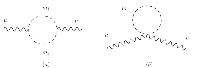
Figure 6: Feynman diagrams with scalar loop-particle

Using the above formulas, the amplitudes of Fig. (6) can be represented as

$$\mathcal{M}_{a}= -\mathcal{C}_{a}\{4B_{22}(p^{2};m_{1},m_{2})g_{\mu\nu}+[B_{0}+4B_{1}+4B_{21}](p^{2};m_{1},m_{2})p_{\mu}p_{\nu}\}$$

$$\mathcal{M}_{b}= \mathcal{C}_{b}A_{0}(m)g_{\mu\nu}$$ (103)

$\mathcal{C}_{a}$ and $\mathcal{C}_{b}$ are the coefficients from the vertexs. We expand and sum the coefficients of the involved graphs.

$$\mathcal{C}_{a}^{WW}= -\frac{1}{2}g^{2}_{2}\sum^{3}_{k=1}(Z^{D*}_{ik}Z^{U}_{jk})\sum^{3}_{l=1}(Z^{U*}_{jl}Z^{D}_{il})$$

$$\mathcal{C}_{b}^{WWD}= \frac{1}{2}g^{2}_{2}\sum^{3}_{k=1}(Z^{D*}_{ik}Z^{D}_{ik})\qquad\mathcal{C}_{b}^{WWU}=\frac{1}{2}g^{2}_{2}\sum^{3}_{k=1}(Z^{U*}_{jk}Z^{U}_{jk})$$

$$\mathcal{C}_{a}^{\gamma\gamma U}= -\frac{4}{9}e^{2}(\sum_{k=1}^{3}Z^{U*}_{ik}Z^{U}_{jk}+\sum_{k=4}^{6}Z^{U*}_{ik}Z^{U}_{jk})^{2}$$

$$\mathcal{C}_{a}^{\gamma\gamma D}= -\frac{1}{9}e^{2}(\sum_{k=1}^{3}Z^{D*}_{ik}Z^{D}_{jk}+\sum_{k=4}^{6}Z^{D*}_{ik}Z^{D}_{jk})^{2}$$

$$\mathcal{C}_{b}^{\gamma\gamma U}= \frac{8}{9}e^{2}(\sum_{k=1}^{3}Z^{U*}_{ik}Z^{U}_{ik}+\sum_{k=4}^{6}Z^{U*}_{ik}Z^{U}_{ik})$$

$$\mathcal{C}_{b}^{\gamma\gamma D}= \frac{1}{18}e^{2}(\sum_{k=1}^{3}Z^{D*}_{jk}Z^{D}_{jk}+\sum_{k=4}^{6}Z^{D*}_{jk}Z^{D}_{jk})$$

$$\widetilde{\mathcal{C}}_{a}^{ZZU}= -\frac{1}{36}[G(1+2c_{2W})\sum^{3}_{k=1}Z^{U*}_{ik}Z^{U}_{jk}-2G(1-c_{2W})\sum^{6}_{k=4}Z^{U*}_{ik}Z^{U}_{jk}]^{2}$$

$$\widetilde{\mathcal{C}}_{a}^{ZZD}= -\frac{1}{36}[G(-2-c_{2W})\sum^{3}_{k=1}Z^{D*}_{ik}Z^{D}_{jk}+G(1-c_{2W})\sum^{6}_{k=4}Z^{D*}_{ik}Z^{D}_{jk}]^{2}$$

$$\widetilde{\mathcal{C}}_{b}^{ZZU}= \frac{1}{18}\{[G(1+2c_{2W})\sum^{3}_{k=1}Z^{U*}_{ik}Z^{U}_{ik}]^{2}+[2G(1-c_{2W})\sum^{6}_{k=4}Z^{U*}_{ik}Z^{U}_{ik}]^{2}\}$$

$$\widetilde{\mathcal{C}}_{b}^{ZZD}= \frac{1}{18}\{[G(-2-c_{2W})\sum^{3}_{k=1}Z^{D*}_{jk}Z^{D}_{jk}]^{2}+[G(1-c_{2W})\sum^{6}_{k=4}Z^{D*}_{jk}Z^{D}_{jk}]^{2}\}$$

$$\widetilde{\mathcal{C}}_{a}^{Z\gamma U}= -\frac{e}{9}(\sum_{k=1}^{3}Z^{U*}_{ik}Z^{U}_{jk}+\sum_{k=4}^{6}Z^{U*}_{ik}Z^{U}_{jk})[G(1+2c_{2W})\sum^{3}_{k=1}Z^{U*}_{ik}Z^{U}_{jk}-2G(1-c_{2W})\sum^{6}_{k=4}Z^{U*}_{ik}Z^{U}_{jk}]^{2}$$

$$\widetilde{\mathcal{C}}_{a}^{Z\gamma D}= -\frac{e}{18}(\sum_{k=1}^{3}Z^{D*}_{ik}Z^{D}_{jk}+\sum_{k=4}^{6}Z^{D*}_{ik}Z^{D}_{jk})[G(-2-c_{2W})\sum^{3}_{k=1}Z^{D*}_{ik}Z^{D}_{jk}+G(1-c_{2W})\sum^{6}_{k=4}Z^{D*}_{ik}Z^{D}_{jk}]^{2}$$

$$\widetilde{\mathcal{C}}_{b}^{Z\gamma U}= \frac{2}{9}e[G(1+2c_{2W})(\sum^{3}_{k=1}Z^{U*}_{ik}Z^{U}_{ik})^{2}-2G(1-c_{2W})(\sum^{6}_{k=4}Z^{U*}_{ik}Z^{U}_{ik})^{2}]$$

$$\widetilde{\mathcal{C}}_{b}^{Z\gamma D}= \frac{1}{9}e[G(-2-c_{2W})(\sum^{3}_{k=1}Z^{D*}_{jk}Z^{D}_{jk})^{2}+G(1-c_{2W})(\sum^{6}_{k=4}Z^{D*}_{jk}Z^{D}_{jk})^{2}]$$

Where, we mark $c_{2W}=c^{2}_{W}-s^{2}_{W}=\cos{2\theta_{W}}$ and

$$\widetilde{\mathcal{C}}^{ZZ}= {c^{\prime}}^{2}\mathcal{C}^{ZZ}-2c^{\prime}s^{\prime}\mathcal{C}^{ZZ^{\prime}}+{s^{\prime}}^{2}\mathcal{C}^{Z^{\prime}Z^{\prime}}$$

$$\widetilde{\mathcal{C}}^{Z\gamma}= c^{\prime}\mathcal{C}^{Z\gamma}-s^{\prime}\mathcal{C}^{Z^{\prime}\gamma}$$ (104)

Appendix B Slef-Energys of Charginos and Neutralinos

For the convenience of batch processing, we divid the calculation results of graphs into two parts $\mathcal{M}_{1}$ and $\mathcal{M}_{2}$:

$$\mathcal{M}= -\int\frac{d^{D}k}{(2\pi)^{D}}tr[A^{\mu}\frac{i}{/\!\!\!k-m_{1}}B^{\nu}\frac{i}{(/\!\!\!k+/\!\!\!q)-m_{2}}]$$

$$(A_{L}B_{L}+A_{R}B_{R})\int\frac{d^{D}k}{(2\pi)^{D}}\frac{1}{d_{0}d_{1}}[2k^{\mu}q^{\mu}+2k^{\nu}q^{\mu}+4k^{\mu}k^{\nu}-2(k^{2}+k\cdot q)g^{\mu\nu}]$$

$$+(A_{L}B_{R}+A_{R}B_{L})\int\frac{d^{D}k}{(2\pi)^{D}}\frac{2m_{1}m_{2}}{d_{0}d_{1}}g^{\mu\nu}$$

Where, $A^{\mu}=A_{L}P_{L}\gamma^{\mu}+A_{R}P_{R}\gamma^{\mu}+$. We define

$$\mathcal{M}_{1}= \mathcal{C}_{1}\int\frac{d^{D}k}{(2\pi)^{D}}\frac{1}{d_{0}d_{1}}[2k^{\mu}q^{\mu}+2k^{\nu}q^{\mu}+4k^{\mu}k^{\nu}-2(k^{2}+k\cdot q)g^{\mu\nu}]$$

$$= i\frac{1-\ln(2\pi)\epsilon}{16\pi^{2}}\mathcal{C}_{1}\{[4B_{22}(q^{2})-2DB_{22}(q^{2})-2B_{21}(q^{2})q^{2}-2B_{1}(q^{2})q^{2}]g^{\mu\nu}$$

$$+4[B_{1}(q^{2})+B_{21}(q^{2})]q^{\mu}q^{\nu}\}$$

$$\mathcal{M}_{2}= \mathcal{C}_{1}\int\frac{d^{D}k}{(2\pi)^{D}}\frac{2m_{1}m_{2}}{d_{0}d_{1}}g^{\mu\nu}$$

$$= i\frac{1-\ln(2\pi)\epsilon}{16\pi^{2}}\mathcal{C}_{2}2m_{1}m_{2}B_{0}(q^{2})g^{\mu\nu}$$

$$\mathcal{C}_{1}= (A_{L}B_{L}+A_{R}B_{R})$$

$$\mathcal{C}_{2}= (A_{L}B_{R}+A_{R}B_{L})$$ (105)

We can analyze their divergences:

$$\mathcal{M}_{1}(q^{2}=0)\sim \frac{i}{16\pi}\mathcal{C}_{1}(m_{1}^{2}+m_{2}^{2})g^{\mu\nu}$$

$$\mathcal{M}_{2}(q^{2}=0)\sim 2\frac{i}{16\pi}\mathcal{C}_{2}m_{1}m_{2}g^{\mu\nu}$$

$$\frac{d\mathcal{M}(q^{2}=0)}{q^{2}}\sim \frac{i}{16\pi}\frac{2}{3}\mathcal{C}_{1}g^{\mu\nu}$$ (106)

We expand and sum the coefficients of the involved graphs.

$$\mathcal{C}_{1}^{WW}= -\frac{c_{W}^{2}G^{2}}{4}[4U^{*}_{j1}N_{i2}N^{*}_{i2}U_{j1}+2U^{*}_{j2}N_{i3}N^{*}_{i3}U_{j2}+2\sqrt{2}(U^{*}_{j1}N_{i2}N^{*}_{i3}U_{j1}+h.c.)$$

$$+4V^{*}_{j1}N_{i2}N^{*}_{i2}V_{j1}+2V^{*}_{j2}N_{i4}N^{*}_{i4}V_{j2}-2\sqrt{2}(V^{*}_{j1}N_{i2}N^{*}_{i4}V_{j2}+h.c.)]$$

$$\mathcal{C}_{2}^{WW}= -\frac{c_{W}^{2}G^{2}}{4}[4U^{*}_{j1}N_{i2}V^{*}_{j1}N_{i2}-2U^{*}_{j2}N_{i3}V^{*}_{j2}N_{i4}-2\sqrt{2}U^{*}_{j1}N_{i2}V^{*}_{j2}N^{*}_{j4}+2\sqrt{2}U^{*}_{j2}N_{i3}V_{i1}N^{*}_{j2}$$

$$+4N^{*}_{j2}U_{1}N^{*}_{j2}V_{i1}+2N^{*}_{j3}U_{i2}N^{*}_{j4}V_{i2}-2\sqrt{2}N^{*}_{j2}U_{i1}N^{*}_{j4}V_{i2}+2\sqrt{2}N^{*}_{j3}U_{i2}N^{*}_{j2}V_{i1}]$$

$$\mathcal{C}_{1}^{\gamma\gamma}= -\frac{e^{2}}{4}[4U^{*}_{j1}U_{i1}U^{*}_{i1}U_{j1}+4U^{*}_{j2}U_{i2}U^{*}_{i2}U_{j2}+4(U^{*}_{j1}U_{i1}U^{*}_{i2}U_{j2}+h.c.)$$

$$+4V^{*}_{j1}V_{i1}V^{*}_{i1}V_{j1}+4V^{*}_{j2}V_{i2}V^{*}_{i2}V_{j2}+4(V^{*}_{j1}V_{i1}V^{*}_{i2}V_{j2}+h.c.)]$$

$$\mathcal{C}_{2}^{\gamma\gamma}= -\frac{e^{2}}{4}[4U^{*}_{j1}U_{i1}V_{j1}V^{*}_{i1}+4U^{*}_{j2}U_{i2}V_{j2}V^{*}_{i2}+4U^{*}_{j1}U_{i1}V_{j2}V^{*}_{i2}+4U^{*}_{j2}U_{i2}V_{j1}V^{*}_{i1}$$

$$+4V^{*}_{j1}V_{i1}U_{j1}U^{*}_{i1}+4V^{*}_{j2}V_{i2}U_{j2}U^{*}_{i2}+4V^{*}_{j1}V_{i1}U_{j2}U^{*}_{i2}+4V^{*}_{j2}V_{i2}U_{j1}U^{*}_{i1}]$$

$$\widetilde{\mathcal{C}}_{1\chi^{\pm}}^{ZZ}= -\frac{G^{2}}{4}[4c_{W}^{4}U^{*}_{j1}U_{i1}U^{*}_{i1}U_{j1}+c_{2W}^{2}U^{*}_{j2}U_{i2}U^{*}_{i2}U_{j2}+2c_{W}^{2}c_{2W}(U^{*}_{j1}U_{i1}U^{*}_{i2}U_{j2}+h.c.)$$

$$+4c_{W}^{4}V^{*}_{j1}V_{i1}V^{*}_{i1}V_{j1}+c_{2W}^{2}2V^{*}_{j2}V_{i2}V^{*}_{i2}V_{j2}+2c_{W}^{2}c_{2W}(V^{*}_{j1}V_{i1}V^{*}_{i2}V_{j2}+h.c.)]$$

$$\widetilde{\mathcal{C}}_{2\chi^{\pm}}^{ZZ}= -\frac{G^{2}}{4}[4c_{W}^{4}U^{*}_{j1}U_{i1}V_{j1}V^{*}_{i1}+c_{2W}^{2}U^{*}_{j2}U_{i2}V_{j2}V^{*}_{i2}+2c_{W}^{2}c_{2W}(U^{*}_{j1}U_{i1}V_{j2}V^{*}_{i2}+h.c.)$$

$$+4c_{W}^{4}V^{*}_{j1}V_{i1}U_{j1}U^{*}_{i2}+c_{2W}^{2}V^{*}_{j2}V_{i2}U_{j2}U^{*}_{i2}+2c_{W}^{2}c_{2W}(V^{*}_{j1}V_{i1}U_{j2}U^{*}_{i2}+h.c.)]$$

$$\widetilde{\mathcal{C}}_{1\chi^{0}}^{ZZ}= -2\frac{G^{2}}{4}(N^{*}_{j3}N_{i3}-N^{*}_{j4}N_{i4})^{2}$$

$$\widetilde{\mathcal{C}}_{2\chi^{0}}^{ZZ}= 2\frac{G^{2}}{4}(N^{*}_{j3}N_{i3}-N^{*}_{j4}N_{i4})^{2}$$

$$\widetilde{\mathcal{C}}_{1}^{Z\gamma}= -\frac{eG}{4}[4c_{W}^{2}U^{*}_{j1}U_{i1}U^{*}_{i1}U_{j1}+2c_{2W}U^{*}_{j2}U_{i2}U^{*}_{i2}U_{j2}+2c_{2W}U^{*}_{j1}U_{i1}U^{*}_{i2}U_{j2}$$

$$+4c_{W}^{2}U^{*}_{j2}U_{i2}U^{*}_{i1}U_{j1}+4c_{W}^{2}V^{*}_{j1}V_{i1}V^{*}_{i1}V_{j1}+2c_{2W}V^{*}_{j2}V_{i2}V^{*}_{i2}V_{j2}$$

$$+2c_{2W}V^{*}_{j1}V_{i1}V^{*}_{i2}V_{j2}+4c_{W}^{2}V^{*}_{j2}V_{i2}V^{*}_{i1}V_{j1}]$$

$$\widetilde{\mathcal{C}}_{2}^{Z\gamma}= -\frac{eG}{4}[4c_{W}^{2}U^{*}_{j1}U_{i1}V_{j1}V^{*}_{i1}+2c_{2W}U^{*}_{j2}U_{i2}V_{i2}V^{*}_{j2}+2c_{2W}U^{*}_{j1}U_{i1}V_{j2}V^{*}_{i2}$$

$$+4c_{W}^{2}U^{*}_{j2}U_{i2}V_{j1}V^{*}_{i1}+4c_{W}^{2}V^{*}_{j1}V_{i1}U_{j1}U^{*}_{i1}+2c_{2W}V^{*}_{j2}V_{i2}U_{j2}U^{*}_{i2}$$

$$+2c_{2W}V^{*}_{j1}V_{i1}U_{j2}U^{*}_{i2}+4c_{W}^{2}V^{*}_{j2}V_{i2}U_{j1}U^{*}_{i1}]$$

References

- (1) [ATLAS], ATLAS-CONF-2023-004.
- (2) M. Ambroso and B. A. Ovrut, Int. J. Mod. Phys. A 26 (2011), 1569-1627 doi:10.1142/S0217751X11052943 [arXiv:1005.5392 [hep-th]].
- (3) P. Fileviez Perez and S. Spinner, Phys. Rev. D 83 (2011), 035004 doi:10.1103/PhysRevD.83.035004 [arXiv:1005.4930 [hep-ph]].
- (4) V. Barger, P. Fileviez Perez and S. Spinner, Phys. Rev. Lett. 102 (2009), 181802 doi:10.1103/PhysRevLett.102.181802 [arXiv:0812.3661 [hep-ph]].
- (5) P. Fileviez Perez and S. Spinner, Phys. Lett. B 673 (2009), 251-254 doi:10.1016/j.physletb.2009.02.047 [arXiv:0811.3424 [hep-ph]].
- (6) J. L. Yang, T. F. Feng and H. B. Zhang, J. Phys. G 47, no.5, 055004 (2020) doi:10.1088/1361-6471/ab7986 [arXiv:2003.09781 [hep-ph]].
- (7) J. L. Yang, H. B. Zhang, C. X. Liu, X. X. Dong and T. F. Feng, JHEP 08, 086 (2021) doi:10.1007/JHEP08(2021)086 [arXiv:2104.03542 [hep-ph]].
- (8) J. L. Yang, T. F. Feng, S. M. Zhao, R. F. Zhu, X. Y. Yang and H. B. Zhang, Eur. Phys. J. C 78, no.9, 714 (2018) doi:10.1140/epjc/s10052-018-6174-5 [arXiv:1803.09904 [hep-ph]].
- (9) J. L. Yang, T. F. Feng, Y. L. Yan, W. Li, S. M. Zhao and H. B. Zhang, Phys. Rev. D 99, no.1, 015002 (2019) doi:10.1103/PhysRevD.99.015002 [arXiv:1812.03860 [hep-ph]].
- (10) J. L. Yang, T. F. Feng, H. B. Zhang, G. Z. Ning and X. Y. Yang, Eur. Phys. J. C 78, no.6, 438 (2018) doi:10.1140/epjc/s10052-018-5919-5 [arXiv:1806.01476 [hep-ph]].
- (11) Z. N. Zhang, H. B. Zhang, J. L. Yang, S. M. Zhao and T. F. Feng, Phys. Rev. D 103, no.11, 115015 (2021) doi:10.1103/PhysRevD.103.115015 [arXiv:2105.09799 [hep-ph]].
- (12) J. L. Yang, T. F. Feng, S. K. Cui, C. X. Liu, W. Li and H. B. Zhang, JHEP 04, 013 (2020) doi:10.1007/JHEP04(2020)013 [arXiv:1910.05868 [hep-ph]].
- (13) J. L. Yang, T. F. Feng and H. B. Zhang, Eur. Phys. J. C 80, no.3, 210 (2020) doi:10.1140/epjc/s10052-020-7753-9 [arXiv:2002.09313 [hep-ph]].
- (14) X. X. Dong, T. F. Feng, H. B. Zhang, S. M. Zhao and J. L. Yang, JHEP 12, 052 (2021) doi:10.1007/JHEP12(2021)052 [arXiv:2106.11084 [hep-ph]].
- (15) X. X. Dong, T. F. Feng, S. M. Zhao and H. B. Zhang, Eur. Phys. J. C 80, no.12, 1206 (2020) doi:10.1140/epjc/s10052-020-08768-0 [arXiv:2005.03351 [hep-ph]].
- (16) X. X. Dong, S. M. Zhao, J. P. Huo, T. T. Wang and T. F. Feng, Phys. Rev. D 109, no.5, 055019 (2024) doi:10.1103/PhysRevD.109.055019 [arXiv:2402.19131 [hep-ph]].
- (17) J. L. Yang, Z. J. Yang, X. Y. Yang, H. B. Zhang and T. F. Feng, Eur. Phys. J. C 83, no.11, 1073 (2023) doi:10.1140/epjc/s10052-023-12235-x
- (18) D. D. Cui, T. F. Feng, Y. L. Yan, H. B. Zhang, G. Z. Ning and J. L. Yang, Phys. Rev. D 102, 075002 (2020) doi:10.1103/PhysRevD.102.075002 [arXiv:2009.09598 [hep-ph]].
- (19) W. Abdallah, A. Hammad, S. Khalil and S. Moretti, Phys. Rev. D 95 (2017) no.5, 055019 doi:10.1103/PhysRevD.95.055019 [arXiv:1608.07500 [hep-ph]].
- (20) C. S. Aulakh, A. Melfo, A. Rasin and G. Senjanovic, Phys. Lett. B 459 (1999), 557-562 doi:10.1016/S0370-2693(99)00708-X [arXiv:hep-ph/9902409 [hep-ph]].
- (21) S. Khalil and H. Okada, Phys. Rev. D 79 (2009), 083510 doi:10.1103/PhysRevD.79.083510 [arXiv:0810.4573 [hep-ph]].
- (22) L. Delle Rose, S. Khalil, S. J. D. King, C. Marzo, S. Moretti and C. S. Un, Phys. Rev. D 96 (2017) no.5, 055004 doi:10.1103/PhysRevD.96.055004 [arXiv:1702.01808 [hep-ph]].
- (23) W. Grimus, L. Lavoura, O. M. Ogreid and P. Osland, Nucl. Phys. B 801, 81-96 (2008) doi:10.1016/j.nuclphysb.2008.04.019 [arXiv:0802.4353 [hep-ph]].
- (24) I. Maksymyk, C. P. Burgess and D. London, Phys. Rev. D 50, 529-535 (1994) doi:10.1103/PhysRevD.50.529 [arXiv:hep-ph/9306267 [hep-ph]].
- (25) G. Cacciapaglia, C. Csaki, C. Grojean and J. Terning, Phys. Rev. D 71, 035015 (2005) doi:10.1103/PhysRevD.71.035015 [arXiv:hep-ph/0409126 [hep-ph]].
- (26) L. Lavoura and J. P. Silva, Phys. Rev. D 47, 2046-2057 (1993) doi:10.1103/PhysRevD.47.2046
- (27) S. Haywood, P. R. Hobson, W. Hollik, Z. Kunszt, G. Azuelos, U. Baur, J. van der Bij, D. Bourilkov, O. Brein and R. Casalbuoni, et al. doi:10.5170/CERN-2000-004.117 [arXiv:hep-ph/0003275 [hep-ph]].
- (28) G. Cacciapaglia, C. Csaki, C. Grojean and J. Terning, Phys. Rev. D 70, 075014 (2004) doi:10.1103/PhysRevD.70.075014 [arXiv:hep-ph/0401160 [hep-ph]].
- (29) C. P. Burgess, S. Godfrey, H. Konig, D. London and I. Maksymyk, Phys. Lett. B 326, 276-281 (1994) doi:10.1016/0370-2693(94)91322-6 [arXiv:hep-ph/9307337 [hep-ph]].
- (30) P. Asadi, C. Cesarotti, K. Fraser, S. Homiller and A. Parikh, Phys. Rev. D 108, no.5, 055026 (2023) doi:10.1103/PhysRevD.108.055026 [arXiv:2204.05283 [hep-ph]].
- (31) H. N. Long and T. Inami, Phys. Rev. D 61, 075002 (2000) doi:10.1103/PhysRevD.61.075002 [arXiv:hep-ph/9902475 [hep-ph]].
- (32) A. Pich, I. Rosell and J. J. Sanz-Cillero, JHEP 01, 157 (2014) doi:10.1007/JHEP01(2014)157 [arXiv:1310.3121 [hep-ph]].
- (33) M. E. Peskin and T. Takeuchi, Phys. Rev. D 46 (1992), 381-409 doi:10.1103/PhysRevD.46.381
- (34) D. C. Kennedy and B. W. Lynn, SLAC-PUB-4608.
- (35) D. Binosi and J. Papavassiliou, Phys. Rept. 479 (2009), 1-152 doi:10.1016/j.physrep.2009.05.001 [arXiv:0909.2536 [hep-ph]].
- (36) S. Hashimoto, J. Kodaira, Y. Yasui and K. Sasaki, Phys. Rev. D 50 (1994), 7066-7076 doi:10.1103/PhysRevD.50.7066 [arXiv:hep-ph/9406271 [hep-ph]].
- (37) A. Denner, G. Weiglein and S. Dittmaier, Nucl. Phys. B 440, 95-128 (1995) doi:10.1016/0550-3213(95)00037-S [arXiv:hep-ph/9410338 [hep-ph]].
- (38) A. Denner, G. Weiglein and S. Dittmaier, Phys. Lett. B 333, 420-426 (1994) doi:10.1016/0370-2693(94)90162-7 [arXiv:hep-ph/9406204 [hep-ph]].
- (39) A. Denner, S. Dittmaier and G. Weiglein, Acta Phys. Polon. B 27, 3645-3660 (1996) [arXiv:hep-ph/9609422 [hep-ph]].
- (40) A. Denner, S. Dittmaier and G. Weiglein, [arXiv:hep-ph/9505271 [hep-ph]].
- (41) J. Papavassiliou and K. Philippides, Phys. Rev. D 48, 4255-4268 (1993) doi:10.1103/PhysRevD.48.4255 [arXiv:hep-ph/9310210 [hep-ph]].
- (42) G. Degrassi and A. Sirlin, Phys. Rev. D 46, 3104-3116 (1992) doi:10.1103/PhysRevD.46.3104
- (43) D. Binosi and J. Papavassiliou, Phys. Rev. D 66, 111901 (2002) doi:10.1103/PhysRevD.66.111901 [arXiv:hep-ph/0208189 [hep-ph]].
- (44) D. Binosi and J. Papavassiliou, J. Phys. G 30, 203 (2004) doi:10.1088/0954-3899/30/2/017 [arXiv:hep-ph/0301096 [hep-ph]].
- (45) J. Papavassiliou and A. Pilaftsis, Phys. Rev. D 53, 2128-2149 (1996) doi:10.1103/PhysRevD.53.2128 [arXiv:hep-ph/9507246 [hep-ph]].
- (46) D. Binosi and J. Papavassiliou, Phys. Rev. D 66, 025024 (2002) doi:10.1103/PhysRevD.66.025024 [arXiv:hep-ph/0204128 [hep-ph]].
- (47) J. Papavassiliou and A. Pilaftsis, Phys. Rev. D 54, 5315-5335 (1996) doi:10.1103/PhysRevD.54.5315 [arXiv:hep-ph/9605385 [hep-ph]].
- (48) J. Papavassiliou, Phys. Rev. D 50 (1994), 5958-5970 doi:10.1103/PhysRevD.50.5958 [arXiv:hep-ph/9406258 [hep-ph]].
- (49) C. P. Burgess, S. Godfrey, H. Konig, D. London and I. Maksymyk, Phys. Rev. D 49, 6115-6147 (1994) doi:10.1103/PhysRevD.49.6115 [arXiv:hep-ph/9312291 [hep-ph]].
- (50) A. Sirlin, Phys. Rev. D 22, 971-981 (1980) doi:10.1103/PhysRevD.22.971
- (51) P. H. Chankowski, S. Pokorski and J. Wagner, Eur. Phys. J. C 47 (2006), 187-205 doi:10.1140/epjc/s2006-02537-3 [arXiv:hep-ph/0601097 [hep-ph]].
- (52) G. Degrassi, B. A. Kniehl and A. Sirlin, Phys. Rev. D 48, R3963-R3966 (1993) doi:10.1103/PhysRevD.48.R3963
- (53) J. de Blas, M. Pierini, L. Reina and L. Silvestrini, Phys. Rev. Lett. 129, no.27, 271801 (2022) doi:10.1103/PhysRevLett.129.271801 [arXiv:2204.04204 [hep-ph]].