HPC Application Parameter Autotuning on Edge Devices: A Bandit Learning Approach

Abstract

The growing necessity for enhanced processing capabilities in edge devices with limited resources has led us to develop effective methods for improving high-performance computing (HPC) applications. In this paper, we introduce $\mathsf{LASP}$ (Lightweight Autotuning of Scientific Application Parameters), a novel strategy designed to address the parameter search space challenge in edge devices. Our strategy employs a multi-armed bandit (MAB) technique focused on online exploration and exploitation. Notably, $\mathsf{LASP}$ takes a dynamic approach, adapting seamlessly to changing environments. We tested $\mathsf{LASP}$ with four HPC applications: Lulesh, Kripke, Clomp, and Hypre. Its lightweight nature makes it particularly well-suited for resource-constrained edge devices. By employing the MAB framework to efficiently navigate the search space, we achieved significant performance improvements while adhering to the stringent computational limits of edge devices. Our experimental results demonstrate the effectiveness of $\mathsf{LASP}$ in optimizing parameter search on edge devices.

I Introduction

Motivation. Edge devices have been gaining popularity as a platform to execute computational workloads for widespread availability and increasing computational power [1]. According to a recent report [2], the market of edge-to-process application data is expected to grow by 75% by 2026. Edge computing processes workload generated by end users nearby, thereby achieving low end-to-end latency and high bandwidth. High-performance computing (HPC) applications are characterized by their need for extensive computational resources and efficient performance. Edge devices can be used for scientific application execution due to their increasing processing capabilities. Recent U.S. DOE and Europe HPC reports [3] outline the opportunities to solve scientific applications on the backdrop of emerging edge computing technologies. However, limited and heterogeneous distributed edge resources present unique challenges to HPC execution on edge devices.

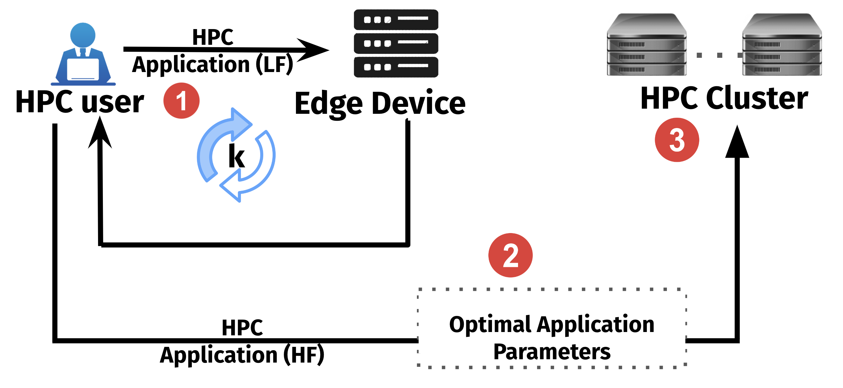
Figure 1: Framework to leverage edge devices to find the optimal parameters to execute applications on HPC clusters.

HPC applications involve complex parameter configurations [4], which significantly affect their performance, contributing towards performance degradation and sometimes even causing non-execution faults [5]. As such, it becomes challenging for the users to evaluate the impact of various tunable parameters on the execution time and understand their effects on each other [6]. Application users must invest considerable effort in searching for the optimal values for all parameters to attain the least execution time [7]. Because manual tuning is time-consuming and labor-intensive and prone to significant error, the automatic tuning of configuration parameters for HPC applications has been a significant subject of study for the past several years [8, 9]. We propose an innovative approach where HPC applications are initially executed on edge devices to determine optimal application-level parameters. The edge devices can efficiently identify the best parameters by running these applications at low fidelity (LF), which demands fewer computational resources. These parameters are then transferred to traditional HPC platforms for execution at high fidelity (HF). This method significantly reduces the time and energy typically spent on parameter tuning on traditional HPC systems, leading to more efficient overall execution of HPC applications. Our approach is illustrated in Fig. 1, where edge devices act as a preliminary stage for parameter optimization before the final execution on HPC clusters.

Notably, existing parameter autotuning techniques have been developed primarily for traditional HPC systems, which themselves demand significant computational resources. Our motivating experiments on four HPC applications on edge devices show the unique challenges HPC parameter autotuning presents on edge platforms. By leveraging edge devices, this paper aims to enhance the efficiency and performance of traditional HPC applications. Our method, based on stochastic techniques for application-level parameters, is portable across various edge and HPC platforms, though some tuning may be required for hardware-level parameters.

Limitations of state-of-the-art approaches. Traditional parameter tuning methods are either exhaustive, time-consuming, or based on heuristics that may not capture the nuances of different application scenarios and the resource-constrained nature and volatility of the edge devices. Existing knowledge-based tuning involves domain experts manually adjusting parameters based on experience and intuition. While this can be effective, it is time-consuming, not scalable, and heavily relies on expert availability, while heuristic approaches utilize rule-based methods [10, 11] to select parameters. These methods are faster but often need more flexibility to adapt to different application needs or changes in the computing environment, and thus, usually get stuck at local optima. Both manual and heuristic methods do not scale well with the increasing complexity of HPC systems [4].

To tackle these challenges, state-of-the-art solutions have employed variants of learning-based approaches [12, 13]. Recently, the effectiveness of configuration autotuning has been demonstrated by more advanced learning techniques such as utilizing machine learning (ML) techniques [14, 15]. However, these models also come with their own overhead costs, making them non-ideal for edge devices. While numerous HPC applications may undergo multiple executions, the input type or size can vary over time. The optimal configuration evolves with changes in input type, input size, or the integration of incremental algorithmic improvements into the application code base [16]. Consequently, the cumulative cost of autotuning increases over time, and autotuning efforts may demand substantial resources on large-scale systems, resulting in the dedication of millions of node hours for autotuning on expensive supercomputers [17]. Simultaneously, the correlation with workload type and input dataset size in big data applications fluctuates, leading to the frequent initiation of time-consuming model retraining tasks [18].

Predictive models can provide quicker solutions but often require substantial training data and are usually limited by the accuracy of their underlying models. They also face challenges in generalizing across different HPC applications and may require retraining for different environments [19]. More importantly, these models are generally static, often leading to suboptimal performance or excessive computational costs [20]. HPC workloads and environments are highly dynamic; therefore, a tuning method that can adapt in real-time to changing conditions is required. However, existing predictive methods do not directly incorporate such dynamic workload in their learning [21].

Many search-based methods [22, 8] achieve satisfactory configuration for many HPC applications. These methods consider the relationship between performance and configuration parameters as a black box technique and employ a specific exploration mechanism to search for the optimal configuration directly. One prominent technique is the Bayesian Optimization (BO). BO-based techniques and their variations can identify a near-optimal configuration with only a limited number of iterations for various HPC applications [23]. However, the BO-based techniques have several limitations – (1) Bayesian optimization struggles with the intricate relationship in big data frameworks, requiring numerous iterations for an accurate model [24]; (2) Vanilla BO prioritizes quick convergence, risking time-consuming sub-optimal configurations due to overlooking evaluation times [21]; and (3) HPC workload characteristics change over time, necessitating configuration re-tuning, while, Vanilla BO lacks historical knowledge utilization and starts afresh for each task [21].

Key Insights and Contributions. To address the limitations of existing approaches, we propose a novel lightweight and online technique for determining the optimal HPC configuration on resource-constrained edge devices: Lightweight Autotuning of Scientific Application Parameters ($\mathsf{LASP}$). We focus on the challenges of configuration selection in HPC for edge devices.

Our solution leverages the multi-arm bandit (MAB) technique, offering unique benefits for HPC applications. First, the flexibility of MAB models allows effective application across various HPC scenarios, adapting to specific needs and constraints. Second, to our knowledge, we are the first to apply this approach to autotuning on edge devices. We compare $\mathsf{LASP}$’s autotuning effectiveness with the default strategy, where applications run with their default settings, demonstrating $\mathsf{LASP}$’s lightweight nature and minimal overhead. Third, MAB models are adaptable, making them suitable for dynamic environments where reward distributions may change over time. This is particularly suitable to the volatile edge environment we are leveraging. Our performance evaluation shows that $\mathsf{LASP}$ can identify the best configuration, significantly enhancing HPC application performance on edge devices. Furthermore, our model dynamically adapts to user needs and changes in application behavior, determining the optimal configuration with minimal regret, thus fulfilling MAB properties.

Organization of the paper. The rest of this paper is organized as follows. In Section II, we present the background and discuss the challenges. In Section III, we formulate the problem and present the objective function. In Section IV, we introduce a lightweight technique for HPC application parameter selection. In Section V, we present results to show performance evaluation in dynamic workload scenarios. In Section VI, we conclude our paper and suggest future directions.

II Preliminaries

II-A Terminology

We first define essential terms that are used throughout the paper. Tunable parameters include the application-level parameters, which can take on various values or states, markedly affecting the execution time of an application.

The autotuning search space, or search space, comprises the extensive $n$-dimensional space created by the range of values that tunable parameters can take. The range of this search space is defined by the potential combinations of tunable parameter configurations, represented by the product of each parameter’s possible values $(a_{1}\texttimes a_{2}\texttimes...\texttimes a_{n}$, where $n$ denotes the number of tunable parameters).

A configuration, or a sample, is a specific combination of parameter values selected within the search space. Sampling or sample evaluation involves running an application using a particular configuration and assessing its runtime. Oracle configuration describes the ideal configuration with minimal execution time or power consumption. While it is intuitive to aim for shorter execution times, we also consider parameter configurations that minimize power consumption of edge device. This is because power is often a limited resource for edge devices, and optimizing for power efficiency is crucial to ensure their effective operation. Identifying the Oracle configuration accurately involves examining all possible configurations in the search space, which is impractical in production settings. However, we conduct an exhaustive search to assess the effectiveness of any given configuration relative to the Oracle configuration. This assessment is quantified as the distance from the Oracle configuration and is defined as follows:

$$\left(\frac{\text{execution time of a configuration}}{\text{execution time of the Oracle configuration}}-1\right)\times 100\%.$$

II-B Multi-Arm Bandit

The multi-arm bandit (MAB) problem [25] is fundamental in probability theory and decision-making under uncertainty. It involves a sequential decision-making framework where an agent must choose with limited information. Pure exploration bandit problems aim to minimize the simple regret, defined as the distance from the optimal solution, as quickly as possible in any given setting. The pure-exploration MAB problem has a long history in the stochastic setting [26], and was recently extended to the non-stochastic setting [27]. Similarly, the stochastic pure-exploration infinite-armed bandit problem was studied by Carpentier et al. [28], where a pull of each arm $i$ yields an i.i.d. sample in $[0,1]$ with expectation $\nu_{i}$, and $\nu_{i}$ is a loss drawn from a distribution with cumulative distribution function $F$. Hyperband [29] works by the best arm identification, i.e., selection of an arm with the highest average payoff in a non-stochastic setting.

The MAB technique has been applied in solving many real-life problems, including exploration and identification of efficient setting from a given distribution. Some application domains include healthcare, finance [30], recommender systems, etc. Naturally, due to their ability to continuously learn and adapt their strategies based on real-time feedback, these approaches have also seen widespread adoption in hyperparameter tuning solutions for neural Networks [31].

In its basic stochastic form, the bandit problem involves a set of $K$ probability distributions, denoted as $\{D_{1},\ldots,D_{K}\}$, each with associated expected values $\{\mu_{1},\ldots,\mu_{K}\}$ and variances $\{\sigma^{2}_{1},\ldots,\sigma^{2}_{K}\}$. Initially, these distributions are unknown to the player. These distributions are often likened to the arms of a slot machine, with the agent acting as a gambler whose goal is to maximize rewards by pulling these arms over multiple turns. At each turn $t=1,2,\ldots$, the player chooses an arm, indexed by $j(t)$, and receives a reward $r(t)\sim D_{j(t)}$. The player’s objective is to determine which distribution has the highest expected value and accumulate as much reward as possible. Bandit algorithms guide the player in choosing an arm $j(t)$ at each turn. The primary metric for evaluating these algorithms is the total expected regret, defined for a given turn $T$ as:

$$R_{T}=T\mu^{*}-\sum_{t=1}^{T}\mu_{j(t)},$$

where $\mu^{*}=\max_{i=1,\ldots,K}\mu_{i}$ is the expected reward from the best arm. Alternatively, the total expected regret can also be expressed as:

$$R_{T}=T\mu^{*}-\mu_{j(t)}\sum_{k=1}^{K}E[T_{k}(T)],$$ (1)

where $T_{k}(T)$ is a random variable denoting the number of times arm $k$ is played during the first $T$ turns.

II-C Edge Devices as a Surrogate for Autotuning

The use of edge devices for running HPC applications is increasingly gaining attention. The Waggle sensor platform [32] is a key example of integrating HPC with edge computing, offering real-time data analysis and modular sensor network capabilities. An extension of this project, The Sage Continuum [33] offers a distributed, software-defined sensor network that leverages machine learning and edge computing and provides a robust framework for real-time data analysis and sensor management. Bhupendra A. Raut et al. [34] provides critical insights into optimizing algorithms for edge-computing sensor systems, particularly focusing on the stability and performance of the blockwise Phase Correlation method in estimating cloud motion vectors. Kim et al. [35] introduces a two-layered scheduling model for edge computing and incorporates “science goals” to align user objectives with resource allocation, thereby offering a nuanced approach to HPC applications in edge systems. The Interconnected Science Ecosystem (INTERSECT) architecture open architecture [36] is a federated instrument-to-edge-to-center framework that advocates autonomous data handling and processing in scientific research. This architecture aligns closely with the objectives of running HPC applications in edge systems and offers a system of systems and microservice architecture for enhanced scalability and adaptability.

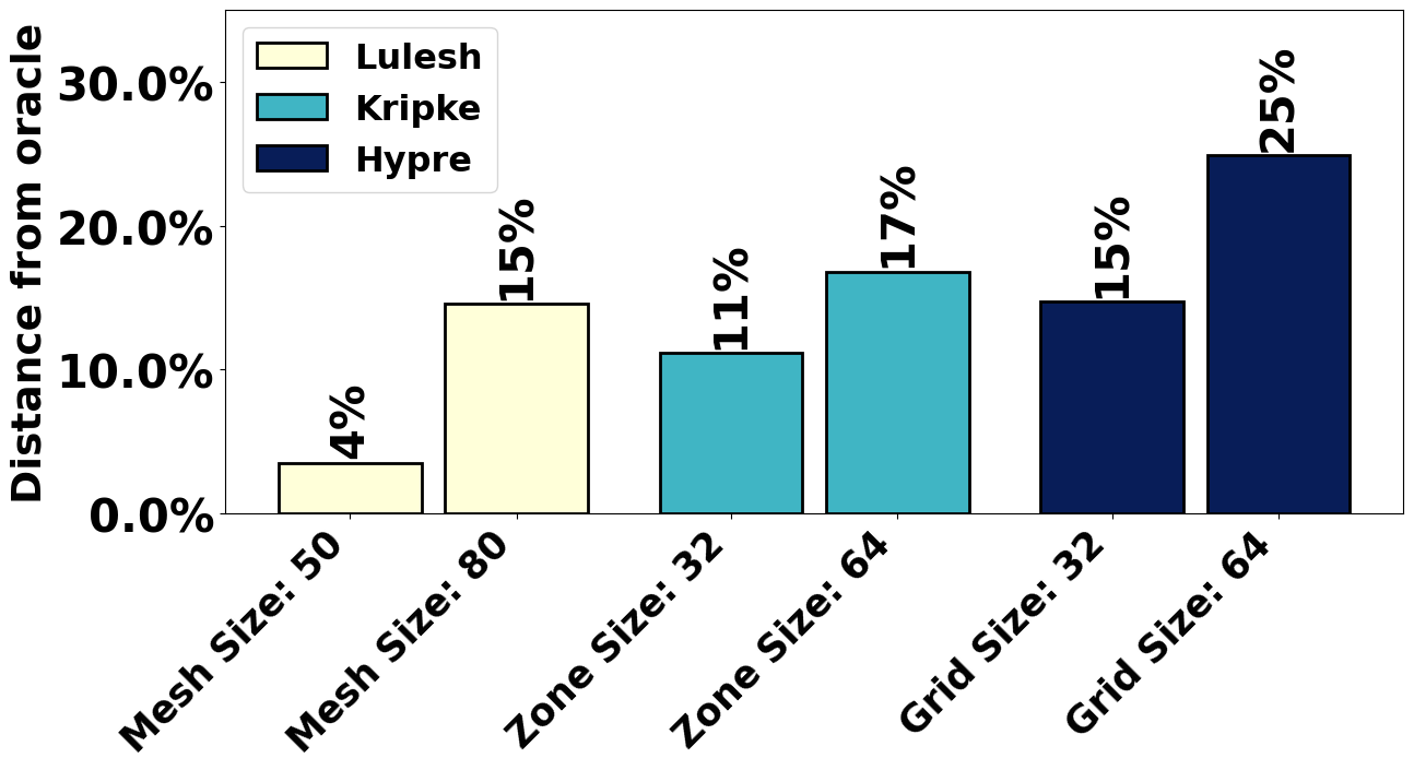
Figure 2: Overlap of optimal configurations on low- and high-fidelity setting. (a) The top 20 configurations identified in the low-fidelity setting are compared to the optimal configuration when run on the high-fidelity setting of the target device, and the average distance between them is measured. (b) The number of common configurations out of top 20 configurations for both the low-fidelity and high-fidelity settings.

By processing data close to the source, edge computing can significantly reduce latency and bandwidth requirements, crucial for time-sensitive HPC applications[37]. Edge devices also enable real-time data processing, which is essential for applications requiring immediate analysis and decision-making. However, these unique advantages present their unique challenges as well. Unlike traditional supercomputing centers, edge devices suffer from limited computational power and memory, posing a challenge for resource-intensive HPC applications. The performance of edge devices can be inconsistent due to their varying specifications and the dynamic nature of edge environments.

Our proposed HF/LF approach is designed to overcome this challenge and accommodate the dynamic nature of HPC workload and edge environment on which we are performing this autotuning task. Notably, our algorithm, $\mathsf{LASP}$, is application-agnostic, meaning it can be employed with any application that associates distinct values with its parameters. In a multi-fidelity context, an application can be executed with varying levels of fidelity settings, such as adjusting the resolution in a numerical simulation or modifying the depth of a machine learning model. For example, the fidelity levels of Hypre is determined by the discretization using $m^{3}$ grid points, where $m$ varies from $m_{\text{min}}=10$ to $m_{\text{max}}=100$. Due to the algebraic multigrid algorithm’s computational complexity of $O(m^{3})$, the mapping from the fidelity parameter $q$ to $m$ is represented as a linear interpolation between $[q_{\text{min}},m^{3}_{\text{min}}]$ and $[q_{\text{max}},m^{3}_{\text{max}}]$. It is to be noted that, there is a trade-off in accuracy due to the shift between low and high fidelity levels, as lower fidelity runs on edge devices are inherently less accurate than those at higher fidelities on traditional HPC systems. However, this trade-off is acceptable, as we are not concerned with the specific results from the low-fidelity runs. Our primary goal is to use these low-fidelity edge device runs to effectively tune the parameters of the model. Importantly, our analysis in Fig. 2 shows that there is a significant overlap between the optimal parameters for both low and high fidelity settings, meaning that the parameters tuned at low fidelity are often effective at high fidelity as well.

We represent fidelity levels using $q\in[q_{\text{min}},q_{\text{max}}]$, where $q_{\text{min}}$ and $q_{\text{max}}$ indicate the minimum and maximum fidelity values, respectively. The time required for function evaluation is assumed to increase linearly with fidelity $q$. To optimize efficiency and reduce tuning costs, we utilize lower fidelity settings on edge devices, leveraging their faster, lower-cost performance. These lower fidelity evaluations, $g(y,q)$ where $q<q_{\text{max}}$, serve as approximations of the high-fidelity objective function, $g(y,q_{\text{max}})$, which runs on traditional HPC systems. The overall goal is to determine the best tuning parameters $y$ to optimize the high-fidelity function $g(y,q_{\text{max}})$ by using the lower fidelity, edge-based evaluations as proxies, thereby improving the efficiency of HPC tuning.

By leveraging this property, $\mathsf{LASP}$ can dynamically navigate the parameter space to identify the optimal configuration, regardless of the specific application. To address the dynamic environment, $\mathsf{LASP}$ incorporates a reward feedback mechanism, enabling the algorithm to operate in real-time and adapt to changing environments. We simulate this dynamic behavior by tuning four HPC applications, and introducing error measurements into our readings, as described in Section V. Furthermore, in the same section, we demonstrate that our algorithm can yield satisfactory results under varying levels of power and CPU capping, underscoring its robustness and adaptability.

In this study, we run applications on varying fidelity settings, for example, Lulesh (mesh size = 50, 80), Kripke (Zone size = 32, 64), and Hypre (Grid size = 32, 64). In Fig. 2(b), we see a significant overlap with the most optimal configurations compared to running them in a low and high-fidelity setting. As shown in Fig. 2(a), we observed that the top 20 configurations identified through low-fidelity simulations and then transferred to a high-fidelity setting achieved performance within 25% of the optimal configuration (oracle) on the target device.

II-D Challenges in HPC Parameter Search

Numerous challenges are associated with attaining an efficient parameter search optimization. First, finding the optimal set of parameters necessitates exhaustive exploration within a vast multidimensional search space. For example, popular HPC applications, such as Kripke [38] and AMG [39], have more than 1 million and 5 million tunable hardware and software parameters, respectively. Searching for the most optimal parameters from this vast set is infeasible without an efficient algorithm. Second, conventional parameter search approaches often yield suboptimal configurations, highlighting the importance of capturing the interplay between application- and hardware-level tuning parameters to achieve maximum performance.

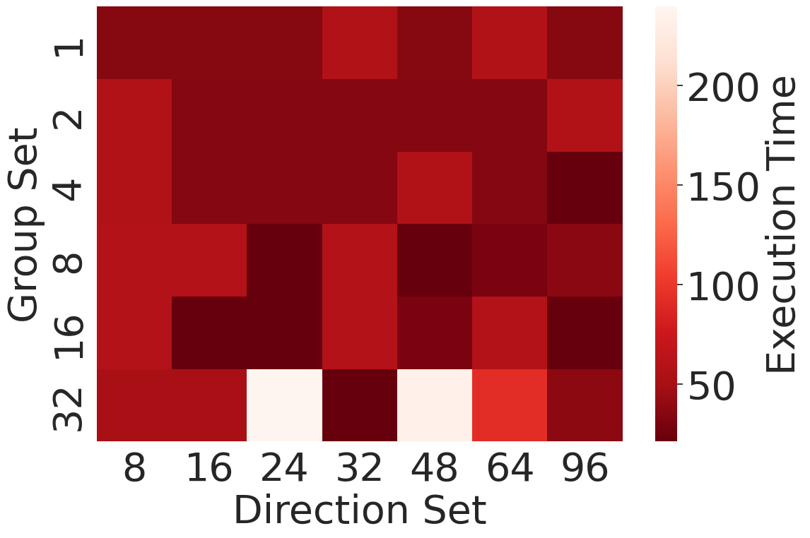
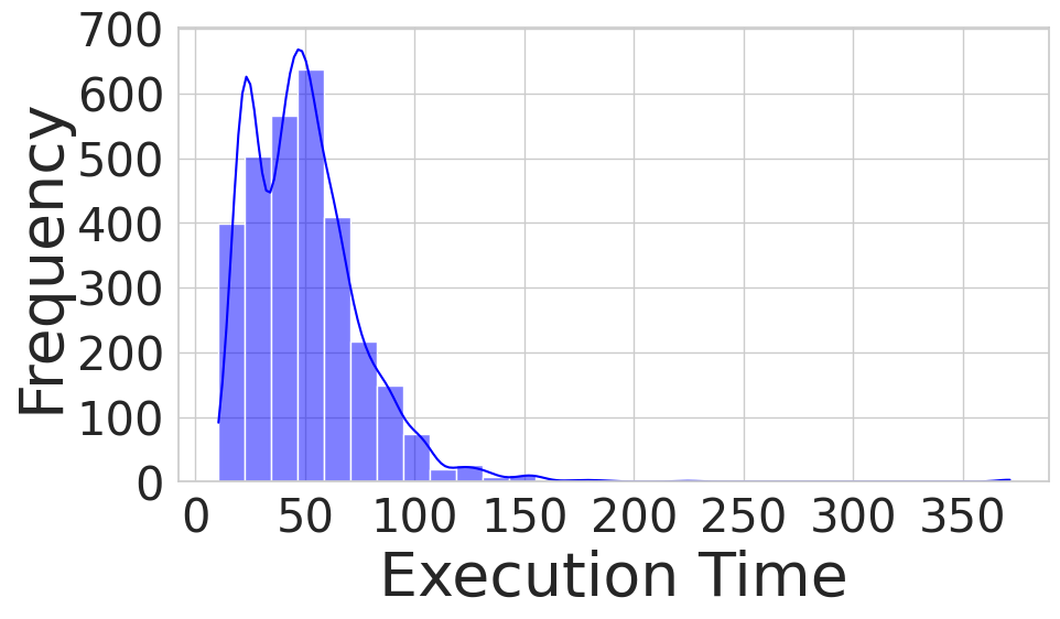
Figure 3: Distribution of execution time for Kripke for all sets of configurations. (a) Tuning only two sets of parameters gives wide variance in the execution time. (b) Distribution of execution time for Kripke for all sets of configurations.

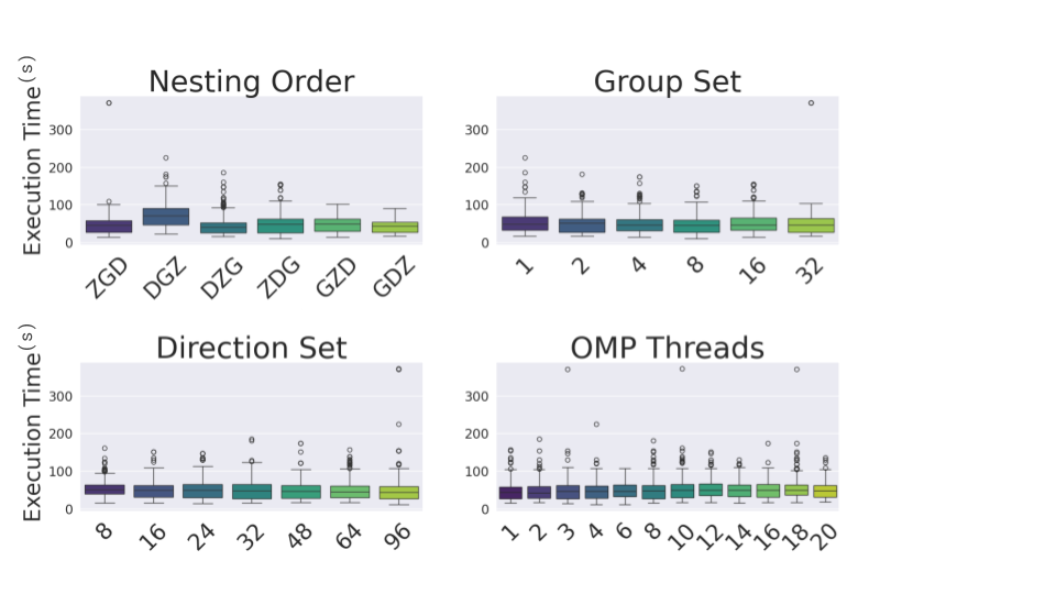
Figure 4: Runtime variability of Kripke for different parameters considered independently.

The significant impact of selecting the right configuration on the application’s execution time is demonstrated in Fig. 3. This figure illustrates the variation in execution times that results from altering only two application-level parameters while keeping all other parameters constant. It is observed that the variance in execution time becomes much more pronounced when more parameters are modified. Fig. 4 illustrates the varying execution times resulting from tuning each parameter individually, reinforcing this key point. Additionally, Fig. 3 provides a distribution of execution times across all sets of configurations.

This clearly highlights the crucial role of proper configuration selection in achieving optimal runtime performance. Considering that most configurations deviate significantly from the absolute best-performing configuration, it is plausible to hypothesize that the challenge posed by a large search space can be mitigated by swiftly discarding the low-performing configurations, namely configurations with high runtimes. However, identifying these areas proves to be a formidable task, often fraught with the risk of overlooking the optimal configuration.

III Problem Formulation

We assume an independently and identically distributed (i.i.d) rewards model, denoted as stochastic bandits. In our model, we assume a choice of $K$ actions, which we refer to as arms, and which are to be executed over $T$ rounds, where $K$ and $T$ are predefined. During every round, the algorithm selects one arm, leading to the accumulation of a reward specific to that arm. The primary objective of the algorithm is to optimize the total reward accumulated throughout the $T$ rounds. The model includes the following assumptions. First, we can only observe the reward associated with the action it chooses and no other information. Specifically, the model needs to be made aware of the potential rewards from other actions that were not selected (a.k.a., bandit feedback [25]). Second, the reward corresponding to each action is i.i.d. For any given action “a”, we assume a reward distribution, $D_{a}$, over the real numbers. Each time we choose an action, its reward is independently drawn from $D_{a}$. Initially, these reward distributions are unknown to the algorithm. Third, we assume that the rewards received in each round are constrained within the range [0, 1].

We include user-defined priorities when selecting the optimal HPC configuration. To include users in the decision framework, we include two parameters – $\alpha$ for execution time and $\beta$ for power consumption, both ranging within [0, 1]. The user can set these parameters to control the optimization balance, e.g., higher values in $\alpha$ and $\beta$ indicate higher emphasis on execution time or power consumption, respectively. In our model, we define $\chi$ as the parameter space, where $\chi=\{1,\ldots,x\}$ is a finite action space; i.e., we set every unique combination of the parameters (configuration) as an arm of the MAB setting.

We specify a distribution $D$ over pairs $(x,~r)$, where $x\in X$ denotes the parameter configuration and $r\in[0,1]^{A}$ denotes a vector of rewards. In its basic stochastic form, our formulation involves a set of $K$ probability distributions for each arm, denoted as $\{D_{1},\ldots,D_{K}\}$, each with associated expected values $\{\mu_{1},\ldots,\mu_{K}\}$ and variances $\{\sigma^{2}_{1},\ldots,\sigma^{2}_{K}\}$. Initially, these distributions are unknown to the algorithm. During each turn $t=1,2,\ldots$, the algorithm chooses an arm, indexed by $j(t)$, and receives a reward $r(t)\sim D_{j(t)}$. The objective is to determine the distribution with the highest expected value and to accumulate as much reward as possible in each iteration.

To model uncertainty, we employ an upper confidence bound (UCB) [40] technique that employs “optimism under uncertainty”. Based on current observations, this technique assumes that every arm represents the best possible outcome. Consequently, the selection of an arm is based on these optimistic estimations. The technique involves initially trying each arm once. Then, for each round, $t=1,\ldots,T$, the technique selects the arm $x(t)$ that appears to be the most promising. The selection of configurations in each iteration is calculated as follows for a configuration $x$ at iteration $t$:

$$UCB(x,t)=R_{x}+\sqrt{\frac{2\ln t}{N_{x}}},$$ (2)

where $R_{x}=f_{\text{reward}}(x)$ is the weighted reward for configuration $x$, and $N_{x}$ is the count of times configuration $x$ has been selected up to iteration $t$. Eq. 2 dynamically balances the exploration of new configurations against exploiting those already known to be effective. The proposed model ensures that the reward is inversely proportional to the normalized metrics of execution time and power consumption, thereby aligning with the user’s optimization goals.

After each iteration $t$, we identify the configuration $x$ with the highest UCB value. The configuration, $x_{t}^{*}$, is determined as follows:

$$x_{t}^{*}=\arg\max_{x}UCB(x,t).$$ (3)

This iterative selection strategy ensures an adaptive balance between exploring untested configurations and exploiting known effective ones. We determine the most frequently selected configuration as follows:

$$x_{\text{opt}}=\arg\max_{x}N_{x}.$$ (4)

After $T$ round of iterations, the algorithm outlined in Section IV outputs the most optimal configuration, $x_{\text{opt}}$. The high-level block diagram of $\mathsf{LASP}$ is given in Fig. 5.

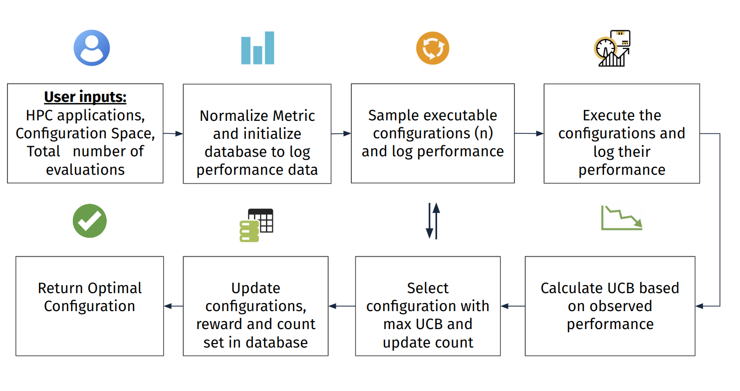
Figure 5: Block diagram of the $\mathsf{LASP}$.

IV Lightweight Autotuning of HPC Application Parameter

Algorithm 1 Lightweight Autotuning of Scientific Application Parameters ($\mathsf{LASP}$)

Input: Configuration space ($\chi$), total iterations ($T$), execution time weight parameter ($\alpha$), and power consumption weight parameter ($\beta$)

1: Initialization: Dictionary for counting selections of each configuration ($N_{x}$), reward metrics ($\tau$ and $\rho$)

2: Apply MinMax normalization: $\tau\leftarrow\frac{\tau-\min(\tau)}{\max(\tau)-\min(\tau)},\rho\leftarrow\frac{\rho-\min(\rho)}{\max(\rho)-\min(\rho)}$

3: for $t\in\{1,2,\ldots,T\}$ do

4:  for configuration $x\in\chi$ do

5:   Calculate weighted reward $R_{x}=w_{\tau}\times\left(\frac{1}{\mu(\tau_{x})}\right)+w_{\rho}\times\left(\frac{1}{\mu(\rho_{x})}\right)$

6:   Calculate UCB values for each configuration using:

7:   $UCB(x,t)=R_{x}+\sqrt{\frac{2\ln t}{N_{x}}}$

8:   end for

9:  Select the configuration, ${x_{t}}^{*}=\arg\max_{x}UCB(x,t)$

10:  Update the selection count $N_{{x^{*},t}}$ = $N_{{x^{*},t}}$ + 1

11:  end for

12: return The optimal configuration ${x_{\text{opt}}}=\arg\max_{x}N_{x}$

Here, we present the details of $\mathsf{LASP}$– a lightweight online HPC application parameter selection algorithm specifically focusing on edge devices. The algorithm is developed based on the MAB framework and tailored to optimize scientific application configurations by balancing execution time and power consumption to facilitate user participation. It systematically explores a defined configuration space, $\chi$, that encompasses all possible combinations of input parameters for the application. The algorithm operates over a set number of iterations, $T$, and is calibrated using user-defined hyperparameters: weights for execution time ($\alpha$) and power consumption ($\beta$). These weights dictate the algorithm’s balance of execution time minimization vs. power consumption reduction. We normalize the execution time ($\tau$) and power consumption ($\rho$) based on the MinMax normalization technique. The normalized execution time $\tau_{\text{x}}$ is calculated as: $\tau_{\text{x}}=\frac{\tau-\tau_{min}}{\tau_{max}-\tau_{min}}$, where $\tau_{min}$ and $\tau_{max}$ are minimum and maximum execution times, respectively. Similarly, the normalized power consumption $\rho_{\text{x}}$ is calculated as: $\rho_{\text{x}}=\frac{\rho-\rho_{min}}{\rho_{max}-\rho_{min}}$, where $\rho_{min}$ and $\rho_{max}$ are minimum and maximum power consumption, respectively. The weighted reward function, $f_{\text{reward}}(x)$, integrates the normalized execution time and power consumption values. The reward for selecting a configuration $x$ at iteration $t$, denoted as $R_{x,t}$, is determined as follows:

$$f_{\text{reward}}(x)=\alpha\times\left(\frac{1}{\mu(\tau_{x})}\right)+\beta\times\left(\frac{1}{\mu(\rho_{x})}\right),$$ (5)

where $R_{x}=f_{\text{reward}}(x)$ is the exploitation term, which is the weighted reward for configuration $x$. Eq. 5 ensures that the reward is inversely proportional to the normalized metrics of execution time and power consumption, thereby aligning with the user’s optimization goals. The UCB in Alg. 1 dynamically balances the exploration of new configurations against exploiting those already known to be effective. The performance of our algorithm is evaluated based on the total reward accrued over $T$ iterations. The expected total reward for a configuration $x$ is determined considering the randomness in execution time, power consumption, and the algorithm’s selection strategy and is defined as follows:

$$\mathbb{E}[R_{x}]=\mathbb{E}\left[\sum_{t=1}^{T}R_{x,t}\right].$$ (6)

The total regret $R_{n}$ after $n$ evaluations of a evaluations with $K$ configurations is bounded by [25]:

$$R_{n}\leq 8\log(n)\sum_{i:\mu_{i}<\mu^{*}}\frac{1}{\Delta_{i}}+\left(1+\frac{\pi^{2}}{3}\right)\left(\sum_{i=1}^{K}\Delta_{i}\right),$$ (7)

where $\mu^{*}$ denotes the highest expected reward (i.e., least execution time) among all configurations, $\mu_{i}$ denotes the expected reward of the $i$-th configuration, and $\Delta_{i}=\mu^{*}-\mu_{i}$ is the difference between the maximum expected reward and the reward of the $i$-th configuration. The bound in Eq. 7 indicates that the regret grows logarithmically with the number of evaluations $n$, which means that the average regret per play $R_{n}/n$ tends to zero as $n$ increases. This demonstrates the efficiency of the UCB-based approach in exploration-exploitation scenarios.

IV-A Integration with Existing Edge Computing Frameworks

$\mathsf{LASP}$ integrates smoothly with existing edge computing frameworks due to its application-agnostic architecture and compatibility with protocols like CoAP (Constrained Application Protocol) [41], enabling efficient communication and coordination between edge devices and HPC systems. However, challenges may arise from hardware differences, dynamic environments, and resource constraints on edge devices, particularly when tuning hardware-level parameters or maintaining real-time feedback. Addressing these requires careful protocol selection and configuration adjustments. As a modular algorithm, LASP can function independently or integrate with existing performance optimization components, as demonstrated in Section 10, showing its effectiveness on devices with varying computational capabilities.

IV-B Challenges of the Proposed Approach

Scalability Limitations: One limitation of $\mathsf{LASP}$ ’s implementation is scalability. As the number of arms (configurations) increases, the UCB algorithm requires exploring a large number of options before it can intelligently determine the optimal configurations. This exploration becomes computationally intensive and inefficient, especially on resource-constrained edge devices.

Network and Coordination issues: The presence of multiple volatile edge devices introduces additional challenges, particularly in terms of network issues. Low communication bandwidths between devices can hinder coordination and data transfer, impacting overall system efficiency.

Scalability with Heterogeneous edge devices: One of the most complex challenges arises when scaling $\mathsf{LASP}$ to handle heterogeneous edge devices. These devices often have varying computational power, memory, and network connectivity, which can impact the effectiveness of a one-size-fits-all algorithm like UCB. Handling diverse device capabilities requires adaptive algorithms that can dynamically adjust resource consumption, depending on the device’s capabilities and environmental constraints. The varying performance characteristics across devices also increase the difficulty of ensuring that optimal configurations are found efficiently for each device. Future iterations of LASP will explore approaches like multi-level parallelism and resource-aware algorithm designs to better handle heterogeneous environments.

V Evaluation

Here, we first discuss details of $\mathsf{LASP}$’s execution, followed by performance evaluation against other configuration selection strategies. We then present how different user-level parameters affect $\mathsf{LASP}$, and finally show how $\mathsf{LASP}$ can adapt to sensitivity changes.

V-A Experimental Setup

We collected experiment data on the NVIDIA Jetson Nano device, a widely-used edge device in research [42] and industry. The device’s compact size, combined with its robust processing capabilities and power efficiency, makes the Jetson Nano a suitable choice for edge computing applications [43].

The Jetson Nano features a 128-core Maxwell GPU and a Quad-core ARM A57 CPU running at 1.43 GHz. It is optimized for efficient parallel processing and computation-intensive tasks. It runs on Ubuntu 20.04 OS and is equipped with 4 GB of 64-bit LPDDR4 RAM with a bandwidth of 25.6 GB/s. It uses a microSD card for storage. The device offers two power modes: MAXN and 5W. In Table I, we provide a detailed description of each mode’s specifications and operating characteristics.

TABLE I: System Specifications for MAXN and 5W Modes

Parameter	MAXN	5W
Power Budget (watts)	10	5
Online CPU	4	2
CPU Max Frequency (MHz)	1479	918
GPU TPC (MHz)	921.6	640

This operational mode mimics the typical power constraints encountered in edge computing scenarios  [44]. The high-fidelity data used in this study was collected on a system featuring an Intel® Core™ i7-14700 vPro® processor, with 20 cores and 28 threads, and a maximum turbo frequency of 5.3 GHz. The system had 64 GB of DDR5 memory and ran on Ubuntu 24.04 LTS.

All the autotuning results and shown in the subsequent section are done on the Jetson Nano device to show the efficacy of our lightweight approach to autotuning. Furthermore, to mitigate potential performance interference, we ensured that no extraneous processes were running on the device, apart from the essential kernel processes and our target HPC applications.

TABLE II: HPC applications’ configuration parameter ranges and their default values.

Application	Parameter Description	Size	Range	Default
kripke	Layout: data layout and kernel implementation details	216	DGZ, DZG, GDZ, GZD, ZDG, ZGD	DGZ
	Gset: number of energy group sets		1, 2, 3, 8, 16, 32	1
	Dset: number of direction sets		8, 16, 32, 48, 64, 96	8
lulesh	r: number of regions to run for each domain	128	1-15	11
	s: number of elements of cube mesh		1-8	8
clomp	partsPerThread: # of independent pieces of work per thread	125	10, 20, 50, 70, 90	10
	zonesPerPart: number of zones		100, 300, 500, 700, 900	100
	zoneSize: bytes in zone		32, 128, 512, 1024, 2048	512
hypre	$P_{x}$, $P_{y}$: Processor grid size (x × y)	92160	1 - 4	2
	strong_threshold: AMG strength threshold		0-1	0.25
	trunc_factor: Truncation factor for interpolation		1-10	2
	P_max_elmts: Max elements per row (AMG)		1-4	1
	coarsen_type: Algorithm for parallel coarsening		1-3	1
	relax_type: Defines which smoother to be used		1-2	1
	smooth_type: Number of smoothing levels		0-1	0
	smooth_num_levels: Smoother level count		1-4	3
	interp_type: Parallel interpolation operator selection		1-3	1
	agg_num_levels: Levels of aggressive coarsening applied		1-10	2

V-B HPC Applications

Table II lists the HPC applications that we used to evaluate the effectiveness of our proposed techniques. To validate our results, we used applications with both small and larger parameter choices, excluding hardware-level parameters such as power and CPU capping. These applications cover a wide-ranging variety of science domains and have been used previously to capture the challenges in autotuning diverse HPC applications [45].

Hypre [46] is a software library for scalable solutions of linear systems, leveraging parallel processing for high-performance computing. It includes the BLOPEX package for solving eigenvalue problems, making it a versatile tool for various scientific applications.

Clomp  [47] is a C-language benchmark that measures OpenMP overheads and performance impacts due to threading, simulating a typical scientific application inner loop workload under strong scaling conditions to assess the efficiency of various OpenMP scheduling algorithms.

Lulesh  [48] is a widely used proxy application that originated from the Shock Hydrodynamics Challenge Problem, designed to test the performance of high-performance computing systems and algorithms, and has since become a benchmark in DOE co-design efforts for exascale computing.

Kripke  [38] is a scalable, 3D deterministic particle transport code that researches the effects of data layout, programming paradigms, and architectures on Sn transport implementation and performance, aiming to optimize solver performance and parallelism.

V-C Execution of $\mathsf{LASP}$

Here, we show how $\mathsf{LASP}$ finds optimal configuration using efficient parameter exploration, where we change the user’s focus on controlling the optimization. We first show how $\mathsf{LASP}$ works when we have control over parameters in two dimensions for Lulesh. Next, we show the results for parameters in three dimensions for the application Kripke and Clomp. We also show the efficacy of $\mathsf{LASP}$ with multi-dimensional parameter application Hypre through our regret analysis and sampling efficiency to find the optimal configuration.

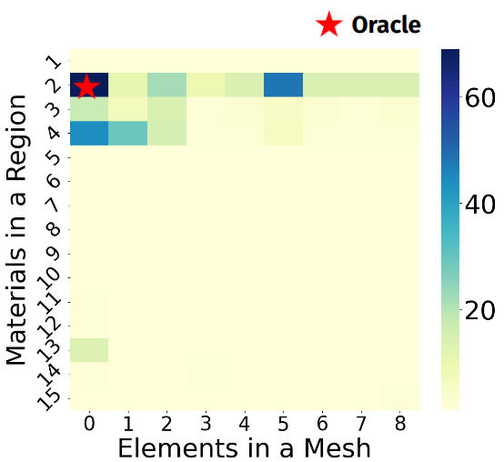
(a) Power Focused

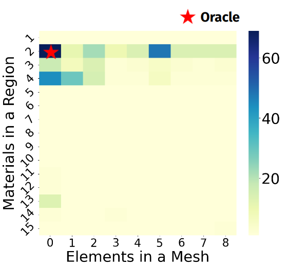
(b) Power Focused

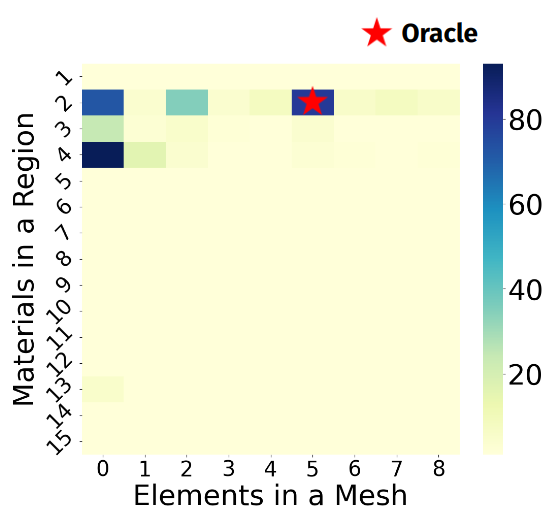
(c) Time Focused

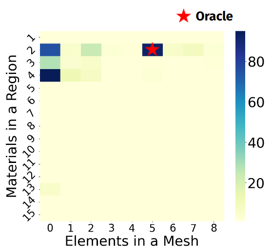
(d) Time Focused

Figure 6: (a) and (b) Exploration of the parameter space with Power as an objective metric for 1000 and 500 iterations, respectively. (c) and (d) Exploration of the parameter space with execution time as an objective metric for 1000 and 500 iterations, respectively.

Efficient Configuration Allocation: In Fig. 6, we show how $\mathsf{LASP}$ achieves the optimal configuration. The figure presents a heatmap visualization of the configuration space for Lulesh, focusing on the application-level parameters “Materials in Region” and “Elements in Mesh.”(The darker the cell, the more frequently LASP selected it as an optimal configuration.) The figure illustrates the frequency of the $\mathsf{LASP}$’s selection of specific configurations – the darker regions indicating a higher selection frequency. We evaluated $\mathsf{LASP}$ over 1000 and 500 iterations, observing that in both scenarios, the algorithm effectively converges towards the optimal configuration. It is important to note, however, that the optimal configuration identified by $\mathsf{LASP}$ may not always be the most optimal, but close to optimal. This is due to $\mathsf{LASP}$’s stochastic nature, which navigates the configuration space based on the reward distribution of configurations. We adapted $\mathsf{LASP}$ to optimize both execution time and power consumption simultaneously. Fig. 6 shows that $\mathsf{LASP}$ effectively explores the configuration space, consistently identifying configurations that balance both objectives. To test its efficiency, we ran $\mathsf{LASP}$ for 500 and 1000 iterations in two representative scenarios. Fig. 6 demonstrates that $\mathsf{LASP}$ converges to optimal configurations efficiently within 500 iterations when the parameter configuration dimensions are small (Lulesh, Kripke, Clomp). Whereas, running $\mathsf{LASP}$ for 1000 iterations helps it explore near-optimal configurations, which is beneficial for portability when deploying on traditional HPC clusters.

We performed a similar analysis for Kripke and Clomp, as shown in Fig. 7. This figure demonstrates the effectiveness and efficiency of $\mathsf{LASP}$ in high-dimensional parameter spaces. In Figs. 7(a) and 7(b), we show how the optimal configuration is selected for Kripke in both time and power-focused experiments, respectively. Similarly, Figs. 7(c) and 7(d) illustrate the efficient convergence of the parameters for Clomp. In both cases, where execution time and power are used as objective metrics, $\mathsf{LASP}$ efficiently converges to the optimal configuration, as indicated by the oracle configuration.

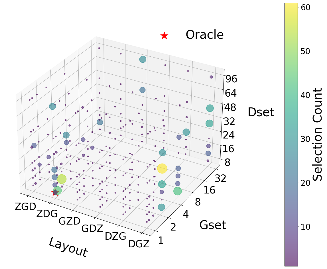
(a) Time Focused

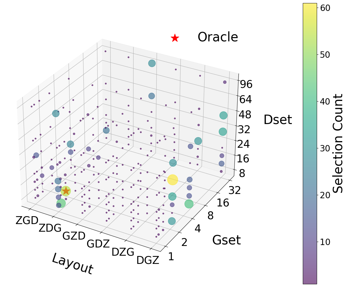
(b) Power Focused

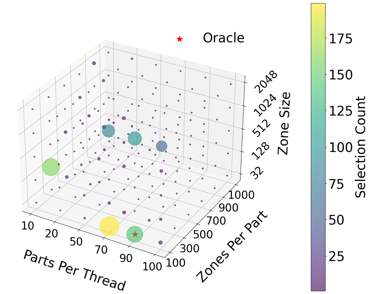
(c) Time Focused

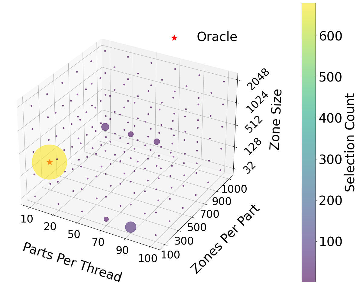
(d) Power Focused

Figure 7: Efficient exploration of the parameter space for Kripke (a & b) and Clomp (c & d).

V-D Performance Evaluation

The default values of parameters of these application have been shown in Table II. We calculate the performance gain under the best configuration $PG_{\text{best}}$ as follows:

$$PG_{\text{best}}=\frac{f_{\text{default}}-f_{\text{best}}}{f_{\text{default}}}\cdot 100\%,$$ (8)

where performance under default configuration is denoted as $f_{\text{default}}$ and the performance under the best configuration is denoted as $f_{\text{best}}$.

In Fig. 8, we do this performance gain analysis of the four applications by varying $\alpha$. At lower $\alpha$, $\mathsf{LASP}$ will work towards finding configurations with lower power consumption. When the user sets the power as the desired objective metric $\mathsf{LASP}$ achieves a 10% performance gain for Clomp, 14% for Lulesh, 9% for Hypre and 6% for Kripke. With increased $\alpha$, $\mathsf{LASP}$ will search the configuration space that yields lower execution time.

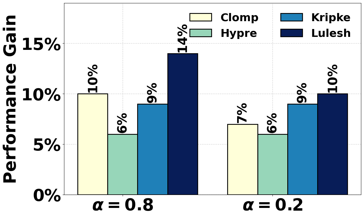
(a) 10W

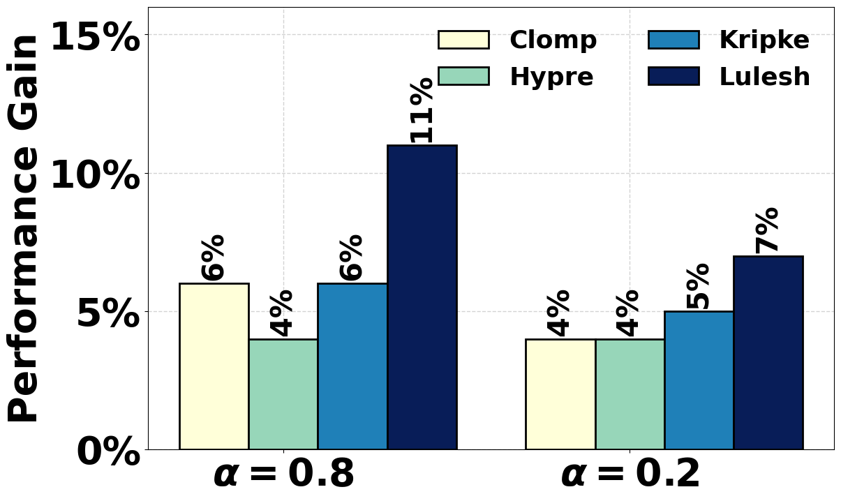
(b) 5W

Figure 8: Performance gain for different applications.

$\mathsf{LASP}$ achieves significant performance gains performance gain in execution time ($\alpha=0.8$) and in power consumption with ($\alpha=0.2$). As expected, $\mathsf{LASP}$ performs better in smaller parameter spaces compared to bigger ones, as shown in Fig. 8. This is because smaller parameter spaces allow for more efficient exploration and convergence to the optimal configuration.

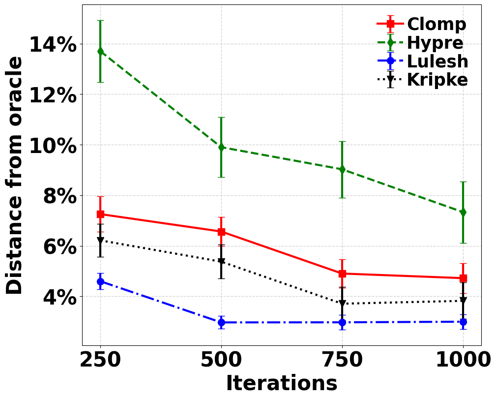
(a) Time Optimized

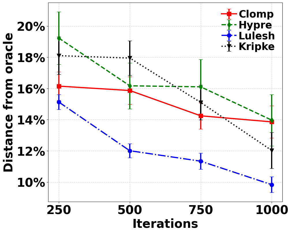
(b) Power Optimized

Figure 9: $\mathsf{LASP}$ reaches closest to the Oracle with very few iterations.

However, $\mathsf{LASP}$’s fast convergence in finding the optimal configuration makes up for its performance in larger parameter spaces. We run $\mathsf{LASP}$ 100 times in order to see the mean distance from the oracle across different runs. The results are demonstrated in Fig. 9 which shows that $\mathsf{LASP}$ can reach within 12% of the optimal configuration even in large parameter spaces, such as those of Hypre, when optimizing for execution time. When optimizing for power consumption, $\mathsf{LASP}$’s performance is less effective compared to when execution time as an objective metric. This is because power consumption is saturated by the edge device when running computationally intensive HPC applications, resulting in a less varied reward metric compared to execution time. As a result, $\mathsf{LASP}$’s ability to converge to the optimal configuration is impacted.

We compared our approach against BLISS [16],a SOTA machine learning-based optimization method that leverages Bayesian Optimization (BO) to minimize tuning expenses. By creating a diverse pool of streamlined models, Bliss accelerates convergence and utilizes surrogate model predictions to streamline the evaluation of configurations, resulting in significant time savings. While we acknowledge our approach, did not do better in terms of efficiently finding the optimal parameters it is because we prioritized a lightweight approach for it to be applicable resource constrained edge devices. This is proved by our analysis of the CPU and memory footprint of using BLISS and LASP for autotuning on two modes (MAXN and 5W) to demonstrate the dynamic nature of our algorithm. A summary of our findings and a description of these two power modes are given in Fig 10.

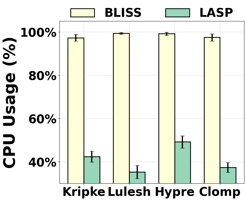
(a) CPU (10W)

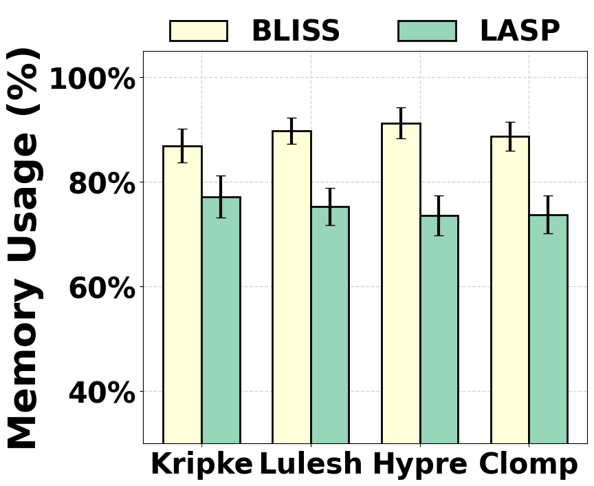
(b) Memory (10W)

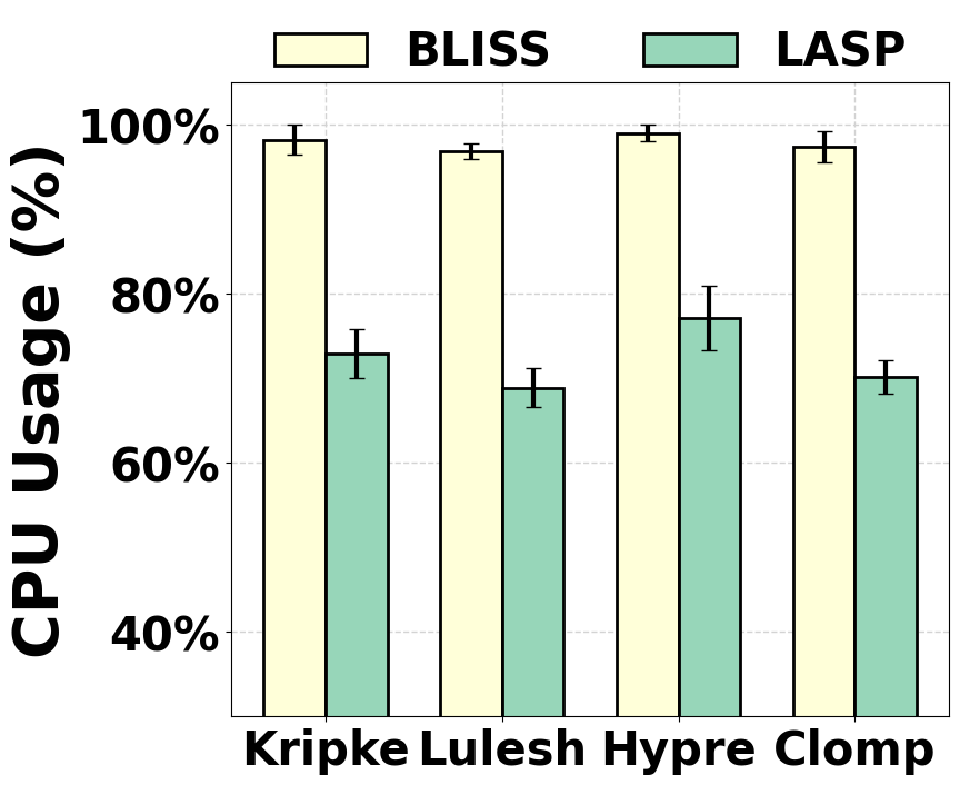
(c) CPU (5W)

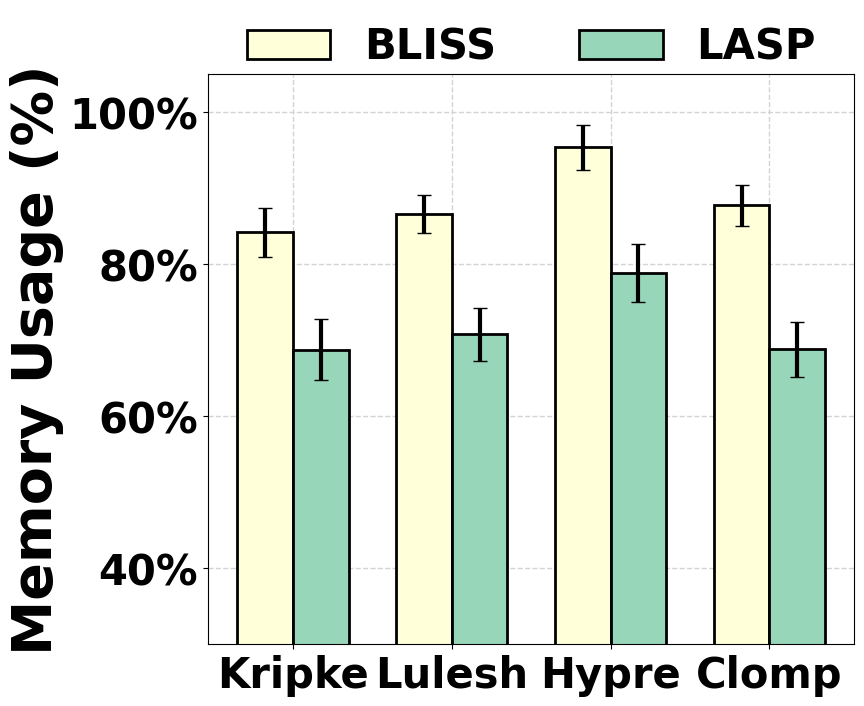
(d) Memory (5W)

Figure 10: Resource Utilization of $\mathsf{LASP}$ compared to BLISS

V-E Regret Analysis

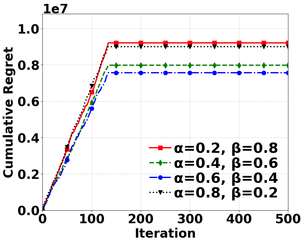
(a) Lulesh

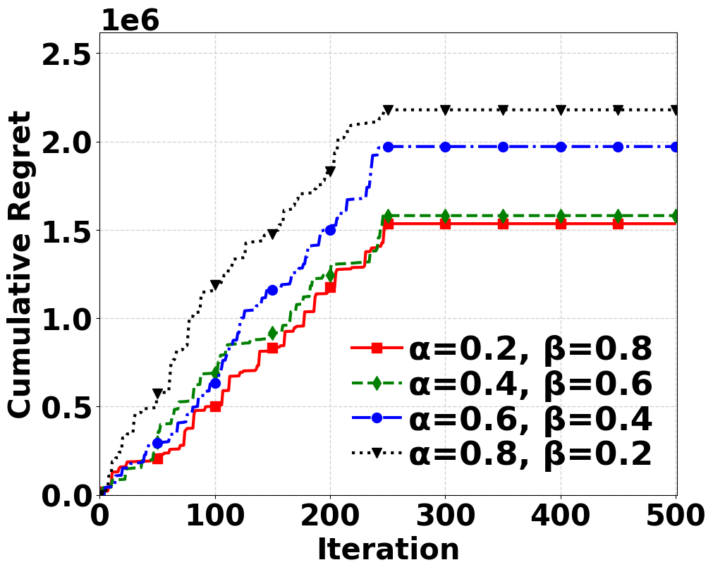
(b) Kripke

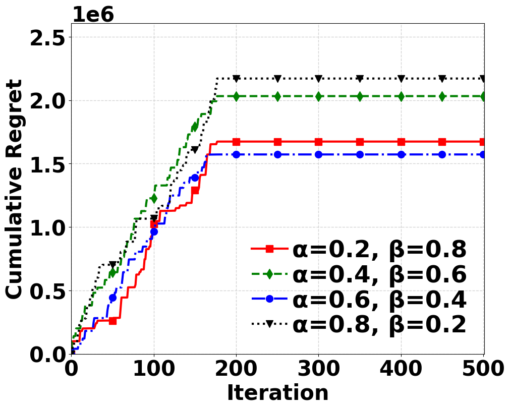
(c) Clomp

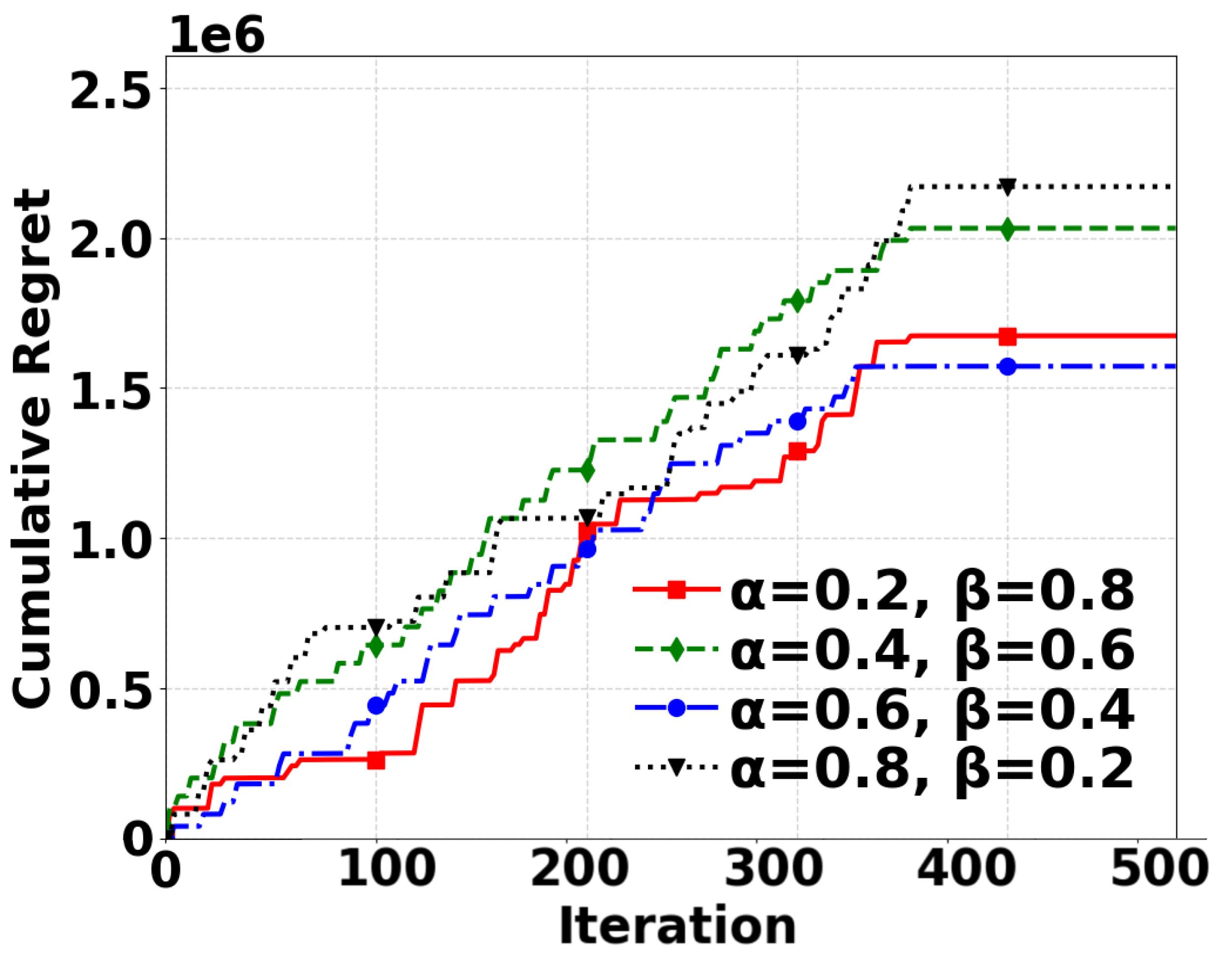
(d) Hypre

Figure 11: Regret analysis for Lulesh, Kripke, Clomp and Hypre.

We evaluate the efficiency of our proposed techniques by performing best-run(one time least regret run) regret analyses, as defined in Equation 1. The results, illustrated in Fig. 11, showcase the convergence of $\mathsf{LASP}$ from an initial trial-and-error phase, characterized by suboptimal decision-making, to optimal configuration selection for four distinct applications. By observing the accumulated regret at each iteration, we notice that the regret saturates after a certain number of iterations for all applications. The number of iterations required to reach minimal regret varies depending on the optimization metric. In the figures, we vary the value of $\alpha$ from 0.8 (time-focused optimization) to 0.2 (power-focused optimization). The plots reveal that $\mathsf{LASP}$ is more effective in finding configurations with shorter execution times. This is due to the variability of the collected data, which makes $\mathsf{LASP}$ better suited for optimizing execution times. As an online MAB-based technique, $\mathsf{LASP}$ navigates the search space based on environmental feedback.

V-F Sensitivity Study

Error in measurement data. We introduce synthetic errors to the measured data to observe the dynamic nature of $\mathsf{LASP}$. To simulate real-world imperfections, we add random noise to our collected data within a range of 5%, 10%, and 15%. As can be seen in Fig. 12, despite the erroneous feedback to $\mathsf{LASP}$, we are still able to achieve considerable performance gains. This resilience can be attributed to the fact that MAB algorithms are inherently adaptive to change due to their design.

In this context, the random noise introduced in our experiments also serves as a proxy for network fluctuation anomalies, such as varying latencies or packet loss, which can lead to inconsistent measurements. Despite these additional challenges, $\mathsf{LASP}$’s ability to adapt to changing conditions allows it to mitigate the impact of such errors and continue to perform well even in the presence of network irregularities.

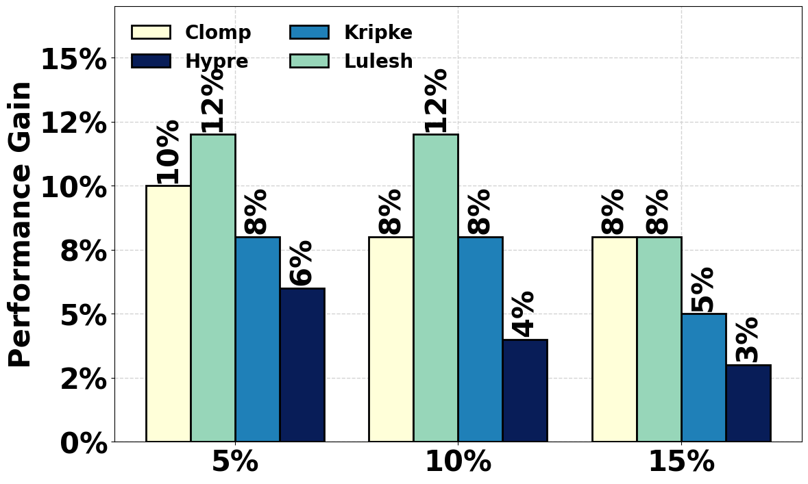
(a) Time Optimized.

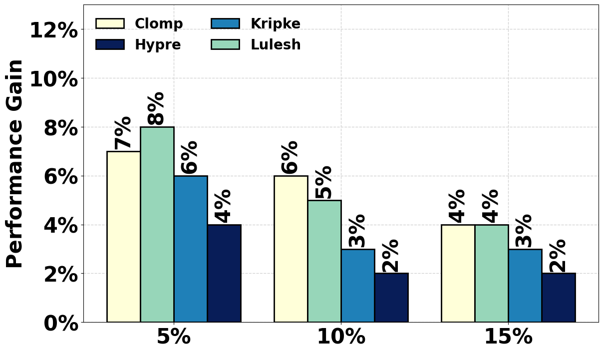
(b) Power Optimized.

Figure 12: Performance analysis with synthetic error in measurement data

VI Concluding Remarks

In this paper, we introduce $\mathsf{LASP}$, a novel and lightweight autotuning approach for dynamic configuration in resource-constrained edge systems. $\mathsf{LASP}$ stands out due to two key enhancements: firstly, it possesses the ability to learn and predict the configuration space in real-time, adapting swiftly to environmental changes. Secondly, it offers customization in optimizing both execution time and power consumption. To assess its effectiveness and efficiency, we conducted extensive experiments on four well-known HPC applications: Lulesh, Kripke, Clomp, and Hypre, each under varying settings. The results consistently demonstrated that $\mathsf{LASP}$ achieved a positive cumulative performance gain in dynamic workload scenarios. This capability is particularly beneficial for leveraging edge devices as proxies to perform the costly autotuning process. Our findings emphasize $\mathsf{LASP}$’s suitability for parameter tuning tasks, especially in environments where workloads frequently change.

VII Acknowledgments

This work is supported in part by the U.S. National Science Foundation under grants CNS-2300124, OAC-2411456, CCF-2324915, and ECCS-2152357. This work was performed under the auspices of the U.S. Department of Energy by Lawrence Livermore National Laboratory under Contract DE-AC52-07NA27344 (LLNL-CONF-855652).

References

- [1] W. Shi, J. Cao, Q. Zhang, Y. Li, and L. Xu, “Edge computing: Vision and challenges,” IEEE internet of things journal, 2016.
- [2] J. Mannik, “Pcie vs. 5g: The importance of hpc at the edge.” https://onestopsystems.com/blogs/one-stop-systems-blog/pcie-vs-5g-the-importance-of-hpc-at-the-edge, 2022.
- [3] P. Beckman et al., “5g enabled energy innovation: Advanced wireless networks for science,” tech. rep., ANL and Northwestern Univ., 2020.
- [4] A. Tiwari, J. K. Hollingsworth, C. Chen, M. Hall, C. Liao, D. J. Quinlan, and Chame, “Auto-tuning full applications: A case study,” Int. J. High Perform. Comput. Appl., 2011.
- [5] Y. Hu, G. Huang, and P. Huang, “Automated reasoning and detection of specious configuration in large systems with symbolic execution,” in (OSDI’20).
- [6] V. Sarkar, W. Harrod, and A. E. Snavely, “Software challenges in extreme scale systems,” in Journal of Physics: Conference Series, vol. 180, p. 012045, IOP Publishing, 2009.
- [7] C. Silvano, G. Agosta, S. Cherubin, D. Gadioli, G. Palermo, A. Bartolini, L. Benini, J. Martinovič, M. Palkovič, K. Slaninová, et al., “The antarex approach to autotuning and adaptivity for energy efficient hpc systems,” in Proc. ACM Int. Conf. Comput. Frontiers, 2016.
- [8] Y. Zhu, J. Liu, M. Guo, Y. Bao, W. Ma, Z. Liu, K. Song, and Y. Yang, “Bestconfig: tapping the performance potential of systems via automatic configuration tuning,” in SoCC ’17, 2017.
- [9] Y. Chen, P. Goetsch, M. A. Hoque, J. Lu, and S. Tarkoma, “d-simplexed: Adaptive delaunay triangulation for performance modeling and prediction on big data analytics,” IEEE Trans. Big Data, 2019.
- [10] S. Kirkpatrick, C. D. Gelatt Jr, and M. P. Vecchi, “Optimization by simulated annealing,” science, vol. 220, no. 4598, pp. 671–680, 1983.
- [11] J. Kennedy and R. Eberhart, “Particle swarm optimization,” in Proceedings of ICNN’95-international conference on neural networks, IEEE.
- [12] T. Chen, T. Moreau, Z. Jiang, L. Zheng, E. Yan, H. Shen, M. Cowan, L. Wang, Y. Hu, L. Ceze, et al., “TVM: An automated End-to-End optimizing compiler for deep learning,” in 13th USENIX Symposium on Operating Systems Design and Implementation (OSDI 18), 2018.
- [13] Z. Bei, Z. Yu, H. Zhang, W. Xiong, C. Xu, L. Eeckhout, and S. Feng, “Rfhoc: A random-forest approach to auto-tuning hadoop’s configuration,” IEEE Trans. Parallel Distrib. Syst., vol. 27, no. 5, 2015.
- [14] S. Cheng, B. Wang, Y. Li, and Y. Guoli, “Efficient performance prediction for apache spark,” 2021.
- [15] Z. Yu, Z. Bei, and X. Qian, “Datasize-aware high dimensional configurations auto-tuning of in-memory cluster computing,” in Proc. 23rd Int. Conf. Archit. Support Prog. Lang. Oper. Syst., pp. 564–577, 2018.
- [16] R. B. Roy, T. Patel, V. Gadepally, and D. Tiwari, “Bliss: auto-tuning complex applications using a pool of diverse lightweight learning models,” in PLDI, 2021.
- [17] P. Balaprakash, J. Dongarra, T. Gamblin, M. Hall, J. K. Hollingsworth, B. Norris, and R. Vuduc, “Autotuning in High-Performance Computing Applications,” Proceedings of the IEEE, vol. 106, Nov. 2018.
- [18] W. M. Sid-Lakhdar, M. M. Aznaveh, X. S. Li, and J. W. Demmel, “Multitask and transfer learning for autotuning exascale applications,” arXiv preprint arXiv:1908.05792, 2019.
- [19] J. J. Thiagarajan, N. Jain, R. Anirudh, A. Gimenez, R. Sridhar, A. Marathe, T. Wang, M. Emani, A. Bhatele, and T. Gamblin, “Bootstrapping parameter space exploration for fast tuning,” in ICS 18, 2018.
- [20] C. Wood, G. Georgakoudis, and D. Beckingsale, “Artemis: Automatic runtime tuning using machine learning,” in ISC 2021, Springer, 2021.
- [21] H. Dou, L. Zhang, Y. Zhang, P. Chen, and Z. Zheng, “Turbo: A cost-efficient configuration-based auto-tuning approach for cluster-based big data frameworks,” J. Parallel Distrib. Comput., vol. 177, 2023.
- [22] R. Krishna, C. Tang, K. Sullivan, and B. Ray, “Conex: Efficient exploration of big-data system configurations for better performance,” IEEE Transactions on Software Engineering, vol. 48, no. 3, 2020.
- [23] H. Dou, P. Chen, and Z. Zheng, “Hdconfigor: automatically tuning high dimensional configuration parameters for log search engines,” IEEE Access, 20.
- [24] J. Xin, K. Hwang, and Z. Yu, “Locat: Low-overhead online configuration auto-tuning of spark sql applications,” in Proceedings of the 2022 International Conference on Management of Data, pp. 674–684, 2022.
- [25] A. Slivkins et al., “Introduction to multi-armed bandits,” Foundations and Trends® in Machine Learning, vol. 12, no. 1-2, pp. 1–286, 2019.
- [26] S. Bubeck, R. Munos, and G. Stoltz, “Pure exploration in finitely-armed and continuous-armed bandits,” Theor. Comput. Sci., 2011.
- [27] K. Jamieson and A. Talwalkar, “Non-stochastic best arm identification and hyperparameter optimization,” in Artif. Intell. Stat., PMLR, 2016.
- [28] A. Carpentier and M. Valko, “Simple regret for infinitely many armed bandits,” in ICML, pp. 1133–1141, PMLR, 2015.
- [29] L. Li, K. Jamieson, G. DeSalvo, A. Rostamizadeh, and A. Talwalkar, “Hyperband: A novel bandit-based approach to hyperparameter optimization,” The Journal of Machine Learning Research, 2017.
- [30] W. Shen, J. Wang, Y.-G. Jiang, and H. Zha, “Portfolio choices with orthogonal bandit learning,” in Twenty-fourth international joint conference on artificial intelligence, 2015.
- [31] J. Snoek, K. Swersky, R. Zemel, and R. Adams, “Input warping for bayesian optimization of non-stationary functions,” in International Conference on Machine Learning, pp. 1674–1682, PMLR, 2014.
- [32] P. Beckman, R. Sankaran, C. Catlett, N. J. Ferrier, R. L. Jacob, and M. E. Papka, “Waggle: An open sensor platform for edge computing,” in 2016 IEEE SENSORS, Orlando, FL, USA, October 30 - November 3, 2016, pp. 1–3, IEEE, 2016.
- [33] N. F. Pete Beckman, “Sage: A distributed software-defined sensor network,” 2013.
- [34] B. A. Raut, P. Muradyan, R. Sankaran, R. C. Jackson, S. Park, S. A. Shahkarami, D. Dematties, Y. Kim, J. Swantek, N. Conrad, et al., “Optimizing cloud motion estimation on the edge with phase correlation and optical flow,” Atmos. Meas. Tech., 2023.
- [35] Y. Kim, S. Park, S. Shahkarami, R. Sankaran, N. Ferrier, and P. Beckman, “Goal-driven scheduling model in edge computing for smart city applications,” Journal of Parallel and Distributed Computing, 2022.
- [36] C. Engelmann, O. Kuchar, S. Boehm, M. J. Brim, T. Naughton, S. Atchley, J. Lange, B. Mintz, and E. Arenholz, “Intersecting needs and challenges in scalable operating system research.” White paper by the U.S. Department of Energy, Jan. 2022.
- [37] A. Hossain and K. Ahmed, “Automating hpc model selection on edge devices,” SC’23, 2023.
- [38] A. J. Kunen, T. S. Bailey, and P. N. Brown, “Kripke-a massively parallel transport mini-app,” tech. rep., Lawrence Livermore National Lab.(LLNL), Livermore, CA (United States), 2015.
- [39] D. F. Richards, O. Aziz, J. Cook, H. Finkel, B. Homerding, T. Judeman, P. McCorquodale, T. Mintz, and S. Moore, “Quantitative performance assessment of proxy apps and parents,” tech. rep., Lawrence Livermore National Lab.(LLNL), Livermore, CA (United States …, 2018.
- [40] P. Auer, “Using confidence bounds for exploitation-exploration trade-offs,” Journal of Machine Learning Research, vol. 3, no. Nov, 2002.
- [41] R. A. Rahman and B. Shah, “Security analysis of iot protocols: A focus in coap,” in 2016 3rd MEC international conference on big data and smart city (ICBDSC), pp. 1–7, IEEE, 2016.
- [42] P. SK, S. A. Kesanapalli, and Y. Simmhan, “Characterizing the performance of accelerated jetson edge devices for training deep learning models,” Proc. ACM Meas. Anal. Comput. Syst., vol. 6, no. 3, 2022.
- [43] M. Lapegna, W. Balzano, N. Meyer, and D. Romano, “Clustering algorithms on low-power and high-performance devices for edge computing environments,” Sensors, vol. 21, no. 16, p. 5395, 2021.
- [44] Y. Li, A.-C. Orgerie, I. Rodero, B. L. Amersho, M. Parashar, and J.-M. Menaud, “End-to-end energy models for edge cloud-based iot platforms: Application to data stream analysis in iot,” Future Gener. Comput. Syst.
- [45] A. Marathe, R. Anirudh, N. Jain, A. Bhatele, J. Thiagarajan, B. Kailkhura, J.-S. Yeom, B. Rountree, and T. Gamblin, “Performance modeling under resource constraints using deep transfer learning,” in Proc. Int. Conf. High Perf. Comput. Netw. Storage Anal., pp. 1–12, 2017.
- [46] R. D. Falgout and U. M. Yang, “hypre: A library of high performance preconditioners,” in Int. Conf. Comput. Sci., Springer, 2002.
- [47] G. Bronevetsky, J. Gyllenhaal, and B. R. De Supinski, “Clomp: Accurately characterizing openmp application overheads,” International journal of parallel programming, vol. 37, pp. 250–265, 2009.
- [48] I. Karlin, J. Keasler, and J. R. Neely, “Lulesh 2.0 updates and changes,” tech. rep., Lawrence Livermore National Lab.(LLNL), 2013.