Fundamental MMSE-Rate Performance Limits of Integrated Sensing and Communication Systems

Abstract

Integrated sensing and communication (ISAC) demonstrates promise for 6G networks; yet its performance limits, which require addressing functional Pareto stochastic optimizations, remain underexplored. Existing works either overlook the randomness of ISAC signals or approximate ISAC limits from sensing and communication (SAC) optimum-achieving strategies, leading to loose bounds. In this paper, ISAC limits are investigated by considering a random ISAC signal designated to simultaneously estimate the sensing channel and convey information over the communication channel, adopting the modified minimum-mean-square-error (MMSE), a metric defined in accordance with the randomness of ISAC signals, and the Shannon rate as respective SAC metrics. First, conditions for optimal channel input and output distributions on the MMSE-Rate limit are derived employing variational approaches, leading to high-dimensional convolutional equations. Second, leveraging variational conditions, a Blahut-Arimoto-type algorithm is proposed to numerically determine optimal distributions and SAC performance, with its convergence to the limit proven. Third, closed-form SAC-optimal waveforms are derived, characterized by power allocation according to channel statistics/realization and waveform selection; existing methods to establish looser ISAC bounds are rectified. Finally, a compound signaling strategy is introduced for coincided SAC channels, which employs sequential SAC-optimal waveforms for channel estimation and data transmission, showcasing significant rate improvements over non-coherent “capacity”. This study systematically investigates ISAC performance limits from joint estimation- and information-theoretic perspectives, highlighting key SAC tradeoffs and potential ISAC design benefits. The methodology readily extends to various metrics, such as estimation rate and the Cramér-Rao Bound.

I Introduction

As next-generation wireless networks are anticipated to accommodate both high-quality sensing and communication (SAC) applications, SAC witness a significant shift from isolation to integration, referred to as integrated sensing and communication (ISAC). ISAC allows wireless devices to conduct data transmission and environmental sensing simultaneously, utilizing the same signals and hardware platform [1, 2, 3, 4]. By leveraging the dual functionality of ISAC, 6G wireless networks significantly enhance their communication reliability, efficiency, and intelligence while addressing the diverse and demanding requirements of various sensing applications.

Research on wireless multiple-input-multiple-output (MIMO) sensing and communication has been conducted in parallel for decades [3, 4]. As landing conditions for ISAC become increasingly mature, there is a pressing need to unfold unified studies for SAC and explore the fundamental theory for ISAC. Pioneering theoretical works [5, 6] on ISAC from estimation- and information-theoretic perspectives derive the Cram$\acute{\textnormal{e}}$r-Rao bound (CRB)-Shannon rate performance bounds for ISAC systems under different setups, with randomness of the transmitted ISAC waveform neglected. An ISAC signal, however, must be random to convey information. [5, 6] simply assume that the sample correlation matrix of the capacity-achieving waveform (i.e., Gaussian waveform) is deterministic, which holds only when the channel coherence time approaches infinity. Consequently, the sensing performance is overly estimated, resulting in unachievable outer bounds that may fail to characterize a practical ISAC system.

Thanks to the foundational work of Xiong et al. [7], a solid framework has been established for analyzing the fundamental tradeoffs in MIMO ISAC systems and revealing the SAC-optimum achieving strategies with random ISAC signals. In alignment with general SAC setups in theoretical studies, the ISAC signal in [7] is modeled as random and known at sensing receivers while remaining unknown to communication receivers. Their work highlights that the SAC tradeoff primarily stems from the degree of randomness of the transmitted ISAC signals and the subspace overlap between sensing and communication channels, providing valuable insights into the intricate SAC interactions within ISAC.

Identifying the ISAC performance limits is crucial for analyzing ISAC systems, understanding the impact of SAC channel parameters, and developing strategies to approach these optimal performances [4, 3, 2]. Achieving this requires solving a family of Pareto multi-objective optimization problems, a complex stochastic functional optimization challenge. The main difficulty lies in the absence of closed-form expressions for the mutual information and the computational complexity of evaluating the expectation of the sensing metric for arbitrary input distributions. While [7] smartly approximates ISAC limits by combining SAC-optimal strategies, this approach provides only loose bounds on the true ISAC limits. As a result, precisely identifying the performance limits of ISAC systems remains an ongoing challenge.

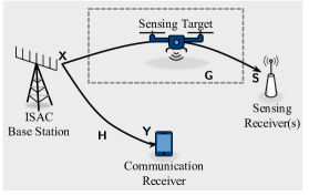
Figure 1: ISAC system model considered in this paper. Plotted is bi-static sensing for demonstration purposes. The sensing receiver(s) can be the ISAC base station itself for mono-static sensing. For the special case of coincided SAC channels, e.g., $\bm{\mathsf{G}}=\bm{\mathsf{H}}$, discussions are delivered in Section III-D.

In order to identify the fundamental limits of MIMO ISAC system, including the SAC performance and their corresponding achieving strategies, the following model is considered in this paper

$$\bm{\mathsf{Y}} =\bm{\mathsf{H}}\bm{\mathsf{X}}+\bm{\mathsf{Z}}_{\rm{c}};$$

$$\bm{\mathsf{S}} =\bm{\mathsf{G}}\bm{\mathsf{X}}+\bm{\mathsf{Z}}_{\rm{s}},$$

where the dual-functional ISAC signal $\bm{\mathsf{X}}$ is emitted from the base station (BS) to convey information over the communication channel $\bm{\mathsf{H}}$ from the received communication signal $\bm{\mathsf{Y}}$, and estimate the sensing channel $\bm{\mathsf{G}}$ from the received sensing signal $\bm{\mathsf{S}}$, as demonstrated in Fig. 1. $\bm{\mathsf{Z}}_{\rm{s}}$ and $\bm{\mathsf{Z}}_{\rm{c}}$ represent respectively the additive noise of the SAC channels. In ISAC configuration, each symbol is random.

Under this setup, the sensing performance of channel estimation is evaluated using the defined modified MMSE ($\epsilon$), with the random ISAC signal $\bm{\mathsf{X}}$ considered a nuisance parameter. More specifically, it is assumed any realization of $\bm{\mathsf{X}}$, denoted as $\bm{X}$, is perfectly known at sensing receiver(s) [7, 8, 5]. $\bm{X}$ serves as a reference signal for sensing purposes. The overall evaluation of sensing performance (i.e., the modified MMSE) involves taking the expectation of MMSE conditioned on $\bm{X}$ over each $\bm{\mathsf{X}}=\bm{X}$ according to the density $p_{\bm{\mathsf{X}}}(\bm{X})$, which is to be determined. Additionally, the communication performance is assessed with the ergodic coherent rate ($\mathcal{R}$), with the assumption of perfect knowledge of each channel realization at the ISAC transmitter [11, Section 10.3].

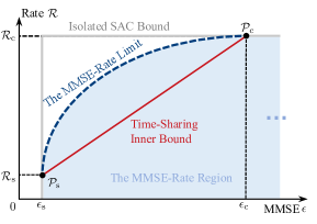
Figure 2: The ISAC MMSE-Rate region: an illustrative plot.

Based on these metrics, this paper further defines the MMSE-Rate Region as the set of achievable MMSE-rate performance pairs utilizing dual-functional ISAC waveform $\bm{\mathsf{X}}$, as illustrated in Fig. 2. The MMSE-Rate limit, i.e., the boundary of the MMSE-Rate Region, represents the optimal Pareto front and should exhibit a similar pattern to that illustrated in Fig. 2. As the endpoints of this limit curve, $\mathcal{P}_{\rm s}(\epsilon_{\rm s},\mathcal{R}_{\rm s})$ and $\mathcal{P}_{\rm c}(\epsilon_{\rm c},\mathcal{R}_{\rm c})$ respectively denote the sensing- and communication-optimal points, and worth more careful investigations [7, 6, 5]. Specifically, $\epsilon_{\rm s}$ represents the best sensing performance regardless of the communication sub-system, while $\mathcal{R}_{\rm s}$ denotes the highest achievable rate when $\epsilon=\epsilon_{\rm s}$. Similarly, $\mathcal{R}_{\rm c}$ denotes the best communication performance regardless of the sensing sub-system, whereas $\epsilon_{\rm c}$ indicates the optimal sensing performance when $\mathcal{R}=\mathcal{R}_{\rm c}$. Therefore, $\mathcal{P}_{\rm s}$ and $\mathcal{P}_{\rm c}$ correspondingly are the SAC-centric ISAC designs [4], while any other points on the limit curve indicate joint SAC design approaches [4] for ISAC systems.

I-A Theoretical Contribution

Based on the aforementioned configuration, the principal theoretical contributions of this paper are summarized as follows.

• The MMSE-Rate limit is investigated in this paper. The conditions for the optimal distributions (e.g., $p_{\bm{\mathsf{X}}}(\bm{X})$ and $p_{\bm{\mathsf{Y}}}(\bm{Y})$) necessary to reach the limit are derived employing a variational calculus approach. The variational conditions can be expressed as complex high-dimensional convolutional equations. A case study on a single-input-single-output (SISO) ISAC channel reveals that the MMSE-Rate limit is unattainable except at $\mathcal{P}_{\rm s}$ and $\mathcal{P}_{\rm c}$, making it an unachievable supremum limit for SISO ISAC.

• Building upon the Blahut-Arimoto framework [12, 13] originally designed for assessing the capacity of discrete memoryless channels, a novel algorithm is proposed to numerically determine the optimal input distribution on the MMSE-Rate limit and compute SAC performance along the limit curve to any desired level of precision. Additionally, the convergence of the proposed algorithm to the MMSE-Rate limit is rigorously proven.

• By considering a sensing channel with multiple widely separated receivers, the SAC performance at $\mathcal{P}_{\rm s}$ and $\mathcal{P}_{\rm c}$ are studied, and corresponding closed-form optimum-achieving waveforms are derived. The optimal waveforms are completely determined by the respective channel (statistics/realizations) and waveform characteristics employed. This paper highlights the water-filling tradeoff (WFT) and the waveform uncertainty tradeoff (WUT) in ISAC, respectively relying on the power allocation and the waveform selection for ISAC signal. Leveraging WFT and WUT, this paper rectifies several loose bounds in [7] for fast evaluation of the MMSE-Rate limit.

• A compound signaling strategy for coincided SAC channels (i.e., when $\bm{\mathsf{G}}=\bm{\mathsf{H}}$) is proposed: the ISAC system first estimates the channel using the sensing-optimal waveform and subsequently conveys information using the communication-optimal waveform over the estimated channel. Leveraging the gain of integrating SAC, this strategy significantly improves the achievable rate compared to the non-coherent “capacity”-achieving strategy.

Additionally, the derived analytical theories are illustrated and verified with numerical examples.

In general, this paper presents a systematic approach to evaluate the MIMO ISAC performance limit and understand its corresponding achieving-strategy in a joint estimation- and information-theoretic perspective. The approach readily adapts to ISAC systems with various metrics, such as the estimation rate [8] and the modified CRB [7, 5, 6].

I-B Notation

Notational convention throughout this paper is as follows unless otherwise specified. $\mathsf{Normal}$ font indicates a random variable, as $\mathsf{x}$, ${\bm{\mathsf{x}}}$, and $\bm{\mathsf{X}}$ respectively represents a random scalar, column vector and matrix, while their deterministic observations or realizations are $italic$, as $x$, x, and $\bm{X}$. $(\cdot)^{*}$, $(\cdot)^{\mathsf{T}}$ and $(\cdot)^{\dagger}$ are respectively the matrix conjugate, transpose and Hermitian operators. ${\rm{rank}}(\cdot)$, ${\rm{Tr}}(\cdot)$ and $\det(\cdot)$ respectively denotes the rank, the trace and the determinant of their matrix argument. $(x)^{+}$ denotes the maximal value of the set $\{0,x\}$. $\mathbb{E}(\cdot)$ is the expectation operator. ${\bm{\mathit{\Sigma}}}_{\!\bm{\mathsf{X}}\bm{\mathsf{Y}}}=\mathbb{E}[({\bm{\mathsf{X}}}-\mathbb{E}{\bm{\mathsf{X}}})({\bm{\mathsf{Y}}}-\mathbb{E}{\bm{\mathsf{Y}}})^{\dagger}]$ denotes the cross covariance matrix between matrices $\bm{\mathsf{X}}$ and $\bm{\mathsf{Y}}$, and ${\bm{\mathit{\Sigma}}}_{\!\bm{\mathsf{X}}}:={\bm{\mathit{\Sigma}}}_{\!\bm{\mathsf{X}}\bm{\mathsf{X}}}$ for simplicity. ${\bm{I}}_{N}$ denotes identity matrix with rank $N$. $\mathbf{0}_{M\times N}$ denote the $M\times N$ matrix whose entries are all 0’s. $\textbf{\em e}_{i}$ denotes the $i$-th standard orthonormal Euclidean basis. The dimensions and subscripts are neglected wherever there is no confusion. $\rm vec(\cdot)$ denotes column-wise stacked vector of its argument. $\otimes$ denotes the Kronecker product operator. ${\bm{\mathit{A}}}\succeq\bm{\mathit{B}}$ implies ${\bm{\mathit{A}}}-\bm{\mathit{B}}$ is positive semidefinite.

I-C Organization

The ISAC system model and SAC performance metrics are introduced and defined in Section II. The main theoretical results for characterizing the MMSE-Rate region are presented in Section III, including the characterization and identification of the MMSE-Rate limit in Sections III-A&III-B, the study of the SAC optimum-achieving strategies in Section III-C, and a novel ISAC signaling strategy when SAC channels coincide in Section III-D. While their corresponding derivations and proofs are in Appendixes. Numerical results are presented in Section IV. Finally, this paper is concluded in Section V.

II System Model

II-A ISAC Signal and System

As shown in Fig. 1, the ISAC BS with $N$ antennas transmits a dual-functional signal $\bm{\mathsf{X}}\in\mathbb{C}^{N\times T}$ for data communication and environmental sensing purposes, where $T\geq N$ is the duration of communication frame as well as the sensing snapshot number. The communication receiver has $N_{\rm{c}}$ receiving antennas, and the sensing receiver has $N_{\rm{s}}$ receiving antennas. The ISAC system can be written as

$$\bm{\mathsf{Y}} =\bm{\mathsf{H}}\bm{\mathsf{X}}+\bm{\mathsf{Z}}_{\rm{c}};$$ (1a)

$$\bm{\mathsf{S}} =\bm{\mathsf{G}}\bm{\mathsf{X}}+\bm{\mathsf{Z}}_{\rm{s}},$$ (1b)

where $\bm{\mathsf{Y}}\in\mathbb{C}^{N_{\rm{c}}\times T}$ is the received communication signal at the communication receiver, $\bm{\mathsf{H}}\in\mathbb{C}^{N_{\rm{c}}\times N}$ is the wireless communication channel, $\bm{\mathsf{S}}\in\mathbb{C}^{N_{\rm{s}}\times T}$ is the received sensing signal at sensing receivers, $\bm{\mathsf{G}}\in\mathbb{C}^{N_{\rm{s}}\times N}$ is the wireless sensing channel (target response/scattering matrix), $\bm{\mathsf{Z}}_{\rm{c}}\in\mathbb{C}^{N_{\rm{c}}\times T}$ and $\bm{\mathsf{Z}}_{\rm{s}}\in\mathbb{C}^{N_{\rm{s}}\times T}$ are the zero mean circular symmetrical complex Gaussian noises to ISAC communication and sensing sub-systems, respectively.

The sensing model (1b) can be equivalently rewritten as

$${\bm{\mathsf{s}}}=\bm{\bar{\mathsf{X}}}{\bm{\mathsf{g}}}+\bm{\mathsf{z}}_{\rm{s}},$$ (1c)

where ${\bm{\mathsf{s}}}=\rm{vec}({\bm{\mathsf{S}}^{\dagger}})$, $\bm{\bar{\mathsf{X}}}={\bm{I}}_{N_{\rm{s}}}\otimes\bm{\mathsf{X}}^{\dagger}$, ${\bm{\mathsf{g}}}=\rm{vec}(\bm{\mathsf{G}}^{\dagger})$ and $\bm{\mathsf{z}}_{\rm{s}}=\rm{vec}(\bm{\mathsf{Z}}_{\rm{s}}^{\dagger})$. The sensing objective in this paper is to estimate the target response ${\bm{\mathsf{g}}}$ instead of estimating all parameters (e.g., distance, Doppler, etc.), which can be extracted from ${\bm{\mathsf{g}}}$’s estimates employing well-designed signal processing algorithms [16]. More information about modeling of $\bm{\mathsf{G}}$ can be seen in [16, 17].

II-B Assumptions

1. General Sensing Channel. The sensing channel ${\bm{\mathsf{g}}}$ follows a zero-mean circular symmetrical complex Gaussian distribution with the (full rank) covariance matrix $\bm{\mathit{\bar{\Sigma}}}_{\!{\bm{\mathsf{g}}}}$, i.e., ${\bm{\mathsf{g}}}\sim\mathcal{CN}(\mathbf{0},\bm{\mathit{\bar{\Sigma}}}_{\!{\bm{\mathsf{g}}}})$. The sensing channel statistics are a priori known [8, 15, 17] at the ISAC base station.

2. Each entry of the communication channel $\bm{\mathsf{H}}$ follows i.i.d. zero-mean circular symmetrical complex Gaussian distribution with a constant variance $\sigma_{\mathsf{h}}^{2}$ [18], i.e., ${\rm{vec}}(\bm{\mathsf{H}})\sim\mathcal{CN}(\mathbf{0},\sigma_{\mathsf{h}}^{2}{\bm{I}}_{NN_{\rm{c}}})$. The communication channel $\bm{\mathsf{H}}$ is known at the ISAC base station.

3. Both the target response matrix $\bm{\mathsf{G}}$ and the communication channel $\bm{\mathsf{H}}$ suffers block fading, which stay constant for a finite duration $T$, and change to a new realization every $T$ symbols in an i.i.d. manner [14]. $T$ is the “coherence time” [19] of both sensing and communication channels.

4. The transmitted signal $\bm{\mathsf{X}}$ has total power budget

   $${{{\rm{Tr}}}(\bm{R}_{\bm{\mathsf{X}}})\leq NP_{0},}$$ (2)

   where $\bm{R}_{\bm{\mathsf{X}}}=\mathbb{E}(\bm{\mathsf{R}}_{\bm{\mathsf{X}}})$ is the statistical correlation matrix of $\bm{\mathsf{X}}$, and $\bm{\mathsf{R}}_{\bm{\mathsf{X}}}=\frac{1}{T}\bm{\mathsf{X}}\bm{\mathsf{X}}^{\dagger}$ is the sample correlation matrix. Equivalently,

   $${\rm{Tr}}(\bm{R}_{\bm{\bar{\mathsf{X}}}})={\rm{Tr}}\left[\mathbb{E}\left(\frac{1}{T}\bm{\bar{\mathsf{X}}}\bm{\bar{\mathsf{X}}}^{\dagger}\right)\right]\leq N_{\rm{s}}NP_{0}.$$ (3)

5. Each element from $\bm{\mathsf{Z}}_{\rm{c}}$ and $\bm{\mathsf{Z}}_{\rm{s}}$ is an i.i.d. zero-mean circular symmetric complex Gaussian random variable with variance $\sigma_{\rm c}^{2}$ and $\sigma_{\rm s}^{2}$, i.e., ${\rm vec}(\bm{\mathsf{Z}}_{\rm{c}})\sim\mathcal{CN}(\mathbf{0},\sigma_{\rm c}^{2}{\bm{I}}_{TN_{\rm{c}}})$ and ${\rm vec}(\bm{\mathsf{Z}}_{\rm{s}})\sim\mathcal{CN}(\mathbf{0},\sigma_{\rm s}^{2}{\bm{I}}_{TN_{\rm{s}}})$, respectively.

6. The transmitted dual-functional random signal $\bm{\mathsf{X}}$ is known at sensing receivers, and stays unknown to the communication receiver(s) [7, 20].

Note (A1) is a general assumption over the sensing channel. A stronger assumption (A1*) for a sensing channel with widely distributed sensing receivers is made in later section. In (A3), flat fading MIMO channels are focused, while the extensions to frequency-selective MIMO channels are straightforward based upon results derived out of this paper. Assumption (A6) is suitable for practical ISAC system, as the sensing receivers typically have the prior knowledge of the transmitted probing signal, while the communication receiver needs to detect and estimate the transmitted signal itself.

The eigenvalue decomposition of $\bm{\mathit{\bar{\Sigma}}}_{\!{\bm{\mathsf{g}}}}$ is

$$\bm{\mathit{\bar{\Sigma}}}_{\!{\bm{\mathsf{g}}}}=\bar{\bm{\mathit{U}}}_{\!{\bm{\mathsf{g}}}}{\bm{\mathit{\bar{\Lambda}}}}_{{\bm{\mathsf{g}}}}\bar{{\bm{\mathit{U}}}}_{\!{\bm{\mathsf{g}}}}^{\dagger},$$ (4)

where $\bar{\bm{\mathit{U}}}_{\!{\bm{\mathsf{g}}}}$ is a unitary matrix with $\bm{\mathit{\bar{\Sigma}}}_{\!{\bm{\mathsf{g}}}}$’s eigenvectors as its columns, and $\bm{\mathit{\bar{\Lambda}}}_{\bm{\mathsf{g}}}={\rm diag}(\lambda_{1},\cdots,\lambda_{NN_{\rm{s}}})$ stores all non-negative eigenvalues of $\bm{\mathit{\bar{\Sigma}}}_{\!{\bm{\mathsf{g}}}}$ on its diagonal.

II-C Sensing and Communication Performance Metrics

II-C1 Sensing

The objective of sensing for an ISAC system is to estimate the wireless sensing channel ${\bm{\mathsf{g}}}$, which is a function of parameters of interest, and the sensing metric is the channel estimation mean square error.

The transmitted waveform $\bm{\mathsf{X}}$ (or $\bm{\bar{\mathsf{X}}}$) is random in order to convey information. In this regard, this paper treats $\bm{\mathsf{X}}$ (or $\bm{\bar{\mathsf{X}}}$) as a nuisance parameter [21, Chapter 10.7], evaluates the sensing performance for each $\bm{\mathsf{X}}=\bm{X}$ (or $\bm{\bar{\mathsf{X}}}=\bar{\bm{X}}$), and takes expectation over the distribution of $\bm{\mathsf{X}}$ (or $\bm{\bar{\mathsf{X}}}$). Conditioned on $\bar{\bm{X}}$, the joint distribution between ${\bm{\mathsf{g}}}$ and ${\bm{\mathsf{s}}}$ is given by

$$\left.\begin{bmatrix}{\bm{\mathsf{g}}}\\ {\bm{\mathsf{s}}}\end{bmatrix}\right|\bar{\bm{X}}\sim\mathcal{CN}\left(\mathbf{0},\begin{bmatrix}\bm{\mathit{\bar{\Sigma}}}_{\!{\bm{\mathsf{g}}}}&\bm{\mathit{\bar{\Sigma}}}_{\!{\bm{\mathsf{g}}}}\bar{\bm{X}}^{\dagger}\\ \bar{\bm{X}}\bm{\mathit{\bar{\Sigma}}}_{\!{\bm{\mathsf{g}}}}&\bar{\bm{X}}\bm{\mathit{\bar{\Sigma}}}_{\!{\bm{\mathsf{g}}}}\bar{\bm{X}}^{\dagger}+\sigma_{\rm s}^{2}{\bm{I}}_{TN_{\rm{s}}}\end{bmatrix}\right).$$ (5)

Note (1c) is a linear model between observations ${\bm{\mathsf{s}}}$ and parameters to be estimated ${\bm{\mathsf{g}}}$. Conditioned on $\bar{\bm{X}}$, the Bayesian MMSE estimator $\hat{{\bm{\mathsf{g}}}}$ of the sensing channel ${\bm{\mathsf{g}}}$ is the conditional mean of ${\bm{\mathsf{g}}}$ on the observed data ${\bm{\mathsf{s}}}$ [21]. Based on (5) and [21, (10.32)], the MMSE estimator of ${\bm{\mathsf{g}}}$ (conditioned on $\bar{\bm{X}}$) is

$$\hat{{\bm{\mathsf{g}}}}|\bar{\bm{X}}=\mathbb{E}({\bm{\mathsf{g}}}|\bar{\bm{X}},{\bm{\mathsf{s}}})=(\sigma_{\rm s}^{2}\bm{\mathit{\bar{\Sigma}}}_{\!{\bm{\mathsf{g}}}}^{-1}+\bar{\bm{X}}^{\dagger}\bar{\bm{X}})^{-1}\bar{\bm{X}}^{\dagger}{\bm{\mathsf{s}}},$$ (6)

and the corresponding MMSE [21, (10.33)] is

$$\mathbb{E}\!\left[\left|\left|(\hat{{\bm{\mathsf{g}}}}|\bar{\bm{X}})-{\bm{\mathsf{g}}}\right|\right|^{2}\right]={{\rm{Tr}}}[(\bm{\mathit{\bar{\Sigma}}}_{\!{\bm{\mathsf{g}}}}^{-1}+\sigma_{\rm s}^{-2}\bar{\bm{X}}^{\dagger}\bar{\bm{X}})^{-1}],$$

which is independent of the observation vector ${\bm{\mathsf{s}}}$.

This paper defines the modified MMSE (as an analogy to the modified CRB [9, 10] in contrast to the conventional CRB for the deterministic parameter estimation task) to be the sensing metric to evaluate the sensing performance over the ensemble contribution of $\bm{\bar{\mathsf{X}}}$, as

$$\epsilon :=\mathbb{E}_{\bm{\bar{\mathsf{X}}}}\left\{{{\rm{Tr}}}\left[\left(\bm{\mathit{\bar{\Sigma}}}_{\!{\bm{\mathsf{g}}}}^{-1}+\sigma_{\rm s}^{-2}{\bm{\bar{\mathsf{X}}}}^{\dagger}{\bm{\bar{\mathsf{X}}}}\right)^{-1}\right]\right\}$$ (7)

$$=\mathbb{E}_{\bm{\mathsf{X}}}\left[\Phi\left({\bm{I}}_{N_{\rm{s}}}\otimes\bm{\mathsf{R}}_{\bm{\mathsf{X}}}\right)\right],$$

where

$$\Phi(\bm{\mathsf{A}}):={\rm{Tr}}\left(\bm{\mathit{\bar{\Sigma}}}_{\!{\bm{\mathsf{g}}}}^{-1}+\frac{T}{\sigma_{\rm s}^{2}}\bm{\mathsf{A}}\right)^{-1}$$

is defined for a matrix $\bm{\mathsf{A}}$ with the same dimension as $\bm{\mathit{\bar{\Sigma}}}_{\!{\bm{\mathsf{g}}}}$.

II-C2 Communication

The objective of communication for an ISAC system is to convey information reliably for data exchange, therefore, a natural communication metric is the data rate, as a measurement of mutual information between transmitted $\bm{\mathsf{X}}$ and received $\bm{\mathsf{Y}}$ per unit time. With each channel realization $\bm{\mathsf{H}}=\bm{H}$ perfectly known at the ISAC transmitter, the ergodic coherent rate is

$$\mathcal{R}:= \ T^{-1}{I(\bm{\mathsf{X}};\bm{\mathsf{Y}}|\bm{\mathsf{H}})}$$ (8)

$$= \ T^{-1}\mathbb{E}_{\bm{\mathsf{H}}}[I(\bm{\mathsf{X}};\bm{\mathsf{Y}}|\bm{\mathsf{H}}=\bm{H})],$$

where $I(\cdot|\cdot)$ denotes the conditional mutual information.

III Main Theoretical Results

In this section, the main theoretical results of this paper are presented. Before delving into theoretical details, this paper first defines the ISAC limits as follows.

The MMSE-Rate performance limit, which gives the maximum rate given the MMSE requirement, or the best MMSE given the rate requirement, is obtained from the following Pareto optimization problem

$$\sup_{p_{\bm{\mathsf{X}}}} \alpha T^{-1}I(\bm{\mathsf{X}};\bm{\mathsf{Y}}|\bm{\mathsf{H}})-(1-\alpha)\mathbb{E}_{\bm{\mathsf{X}}}\left[\Phi({\bm{I}}_{N_{\rm{s}}}\otimes\bm{\mathsf{R}}_{\bm{\mathsf{X}}})\right]$$ (9)

$$\rm{s.t.} \bm{\mathsf{R}}_{\bm{\mathsf{X}}}=\bm{\mathsf{R}}_{\bm{\mathsf{X}}}^{\dagger},\ \bm{\mathsf{R}}_{\bm{\mathsf{X}}}\succeq\mathbf{0},\ {{\rm{Tr}}}\left[\mathbb{E}_{\bm{\mathsf{X}}}\left(\bm{\mathsf{R}}_{\bm{\mathsf{X}}}\right)\right]=NP_{0},$$

where $\alpha\in[0,1]$ blends the weight between sensing and communication. E.g., $\alpha=0$ indicates a sensing-only optimization, corresponding to the sensing-centric ISAC designs. Conversely, $\alpha=1$ indicates a communication-only optimization, corresponding to the communication-centric ISAC designs. For general $\alpha\in(0,1)$, (9) is a weighted optimization problem for SAC co-design. (9) is a complicated stochastic optimization [22, Chapter 102] problem. It is stochastic because the optimization is involved with $\bm{\mathsf{H}}$, i.e., the Reighlay fading communication channel. To solve this kind of problem, the sample average approximation (SAA) method [23] can be adopted, which solves the following optimization problem with each realization of $\bm{\mathsf{H}}=\bm{H}$

$$\sup_{p_{\bm{\mathsf{X}}}} \frac{\alpha}{T}I(\bm{\mathsf{X}};\bm{\mathsf{Y}}|\bm{\mathsf{H}}=\bm{H})\!-\!(1-\alpha)\mathbb{E}_{\bm{\mathsf{X}}}\!\left[\Phi({\bm{I}}_{N_{\rm{s}}}\otimes\bm{\mathsf{R}}_{\bm{\mathsf{X}}})\right]$$ (10)

$$\rm{s.t.} \bm{\mathsf{R}}_{\bm{\mathsf{X}}}=\bm{\mathsf{R}}_{\bm{\mathsf{X}}}^{\dagger},\ \bm{\mathsf{R}}_{\bm{\mathsf{X}}}\succeq\mathbf{0},\ {{\rm{Tr}}}\left[\mathbb{E}_{\bm{\mathsf{X}}}\left(\bm{\mathsf{R}}_{\bm{\mathsf{X}}}\right)\right]=NP_{0},$$

and takes expectation of the optimized results with the distribution of $\bm{\mathsf{H}}$ to yield the solution to (9). The proof of convergence of SAA method can be found in [23].

For any given $\alpha\in[0,1]$ and $\bm{H}$, problem (10) is a complicated functional multi-objective optimization problem. It is functional because the optimization is with respect to the channel input distribution, i.e., the PDF $p_{\bm{\mathsf{X}}}(\bm{X},\alpha)$. Once the optimal distributions $p_{\bm{\mathsf{X}}}^{\star}(\bm{X},\alpha)$ and $p_{\bm{\mathsf{Y}}}^{\star}(\bm{Y},\alpha)=\int p_{\bm{\mathsf{X}}}^{\star}(\bm{X},\alpha)p_{\bm{\mathsf{Z}}_{\rm{c}}}(\bm{Y}-\bm{H}\bm{X})\mathsf{d}\bm{X}$ are obtained by solving (10), the SAC performance are respectively given by

$$\tilde{\mathcal{R}}(\alpha) =\frac{1}{T}\left[-\int p_{\bm{\mathsf{Y}}}^{\star}(\bm{Y},\alpha)\log p_{\bm{\mathsf{Y}}}^{\star}(\bm{Y},\alpha)\mathsf{d}\bm{Y}-h(\bm{\mathsf{Z}}_{\rm{c}})\right];$$

$$\tilde{\epsilon}(\alpha) =\mathbb{E}_{\bm{\mathsf{X}}}\left[\Phi\left({\bm{I}}_{N_{\rm{s}}}\otimes\bm{\mathsf{R}}_{\bm{\mathsf{X}}}\right)\right],$$

where $h(\bm{\mathsf{Z}}_{\rm{c}})$ is the differential entropy of the communication noise. Note that $\tilde{\mathcal{R}}(\alpha)$ and $\tilde{\epsilon}(\alpha)$ are a function of communication channel realization $\bm{H}$. Therefore, according to the principle of SAA, the overall SAC performances are

$$\mathcal{R}(\alpha) =\mathbb{E}_{\bm{\mathsf{H}}}[\tilde{\mathcal{R}}(\alpha)];$$

$$\epsilon(\alpha) =\mathbb{E}_{\bm{\mathsf{H}}}[\tilde{\epsilon}(\alpha)].$$

Finally, the MMSE-Rate performance limit is the set of all MMSE-Rate pairs

$$\left\{(\epsilon(\alpha),\mathcal{R}(\alpha))|\alpha\in[0,1]\right\},$$ (11)

and the MMSE-Rate performance region is the set of all MMSE-Rate pairs

$$\left\{(\epsilon,\mathcal{R})|\mathcal{R}\leq\mathcal{R}(\alpha)\text{ and }\epsilon\geq\epsilon(\alpha),\exists\alpha\in[0,1]\right\}.$$ (12)

Consequently, to obtain the MMSE-Rate performance limit and investigate the operational region of practical ISAC systems, (10) should be solved first.

III-A Identifying The MMSE-Rate Performance Limit

To identify the ISAC limits, this paper adopts variational methods to solve for the optimal distribution along the entire MMSE-Rate performance limit curve, i.e., $\forall\alpha\in[0,1]$. The conditions for the optimal distribution along the MMSE-Rate curve are summarized in Theorem 1.

Theorem 1

Given a communication channel realization $\bm{\mathsf{H}}=\bm{H}$:

1. When $\alpha\in(0,1]$, the optimal output distribution $p_{\bm{\mathsf{Y}}}^{\star}(\bm{Y},\alpha)$ must satisfy

   $$\hskip-17.07182pt\int\!\!p_{\bm{\mathsf{Z}}_{\rm{c}}}(\bm{Y}-\!\bm{H}\bm{X})\log p_{\bm{\mathsf{Y}}}^{\star}(\bm{Y},\alpha)\mathsf{d}\bm{Y}\!\!=T(1-\frac{1}{\alpha}){\rm{Tr}}\!\!\left(\!\!\bm{\mathit{\bar{\Sigma}}}_{\!{\bm{\mathsf{g}}}}^{-1}\!\!\!+\!\frac{1}{\sigma_{\rm s}^{2}}{\bm{I}}_{N_{\rm{s}}}\!\otimes\bm{X}\bm{X}^{\dagger}\right)^{\!\!-1}\!\!\!\!\!\!+\mu_{1}(\alpha)+\mu_{2}(\alpha){\rm{Tr}}(\bm{X}\bm{X}^{\dagger})\quad\forall\bm{X}\in\mathbb{C}^{N\times T}\!,$$ (13)

   where $\mu_{1}(\alpha)$ and $\mu_{2}(\alpha)$ are chosen to make sure

   $$\int p_{\bm{\mathsf{X}}}^{\star}(\bm{X},\alpha)\mathsf{d}\bm{X}=1;$$ (14a)

   $$\int{\rm{Tr}}(\bm{X}\bm{X}^{\dagger})p_{\bm{\mathsf{X}}}^{\star}(\bm{X},\alpha)\mathsf{d}\bm{X}=TNP_{0}.$$ (14b)

2. When $\alpha=0$, a sufficient condition for the optimal input distribution $p_{\bm{\mathsf{X}}}^{\star}(\bm{X},0)$ is that it preserves a constant sample correlation matrix.

Proof:

See Appendix A. ∎∎

Based on (13), the optimal output distribution $p_{\bm{\mathsf{Y}}}^{\star}(\bm{Y},\alpha)$ can be calculated using multi-dimensional complex Hermite transform. However, due to the large dimensionality of the signal space, obtaining $p_{\bm{\mathsf{Y}}}^{\star}(\bm{Y},\alpha)$ (and hence, $p_{\bm{\mathsf{X}}}^{\star}(\bm{X},\alpha)$) in general case is typically unprocurable. It makes the performance limit-achieving distribution along the performance limit curve hard to interpret. Rather, Theorem 1 can be effective in checking whether any given distribution is on the MMSE-Rate performance limit.

To dig insights on the distribution to achieve the MMSE-Rate performance limit, i.e., how the distribution of the input signal will affect the SAC performance, this paper now considers a simpler case.

III-A1 Case Study on the MMSE-Rate Performance Limit for Fast-Fading SISO ISAC Channel

To enhance understanding of the limit-achieving distribution, this paper now considers the case with $N=N_{\rm{s}}=N_{\rm{c}}=1$ and $T=1$, i.e., a fast-fading SISO channel, although numerical approach can be applied in the same fashion to solve problem (10) in high-dimensional space. With this simplification, the channel model (1) reduces to

$$\mathsf{y=hx+z}_{\rm c};$$ (15a)

$$\mathsf{s=gx+z}_{\rm s},$$ (15b)

where $\mathsf{h}\sim\mathcal{N}(0,\sigma_{\mathsf{h}}^{2})$ according to assumption (A2), $\mathsf{g}\sim\mathcal{N}(0,\sigma_{\mathsf{g}}^{2})$ according to assumption (A1), $\mathsf{z}_{\rm c}\sim\mathcal{N}(0,\sigma_{\rm c}^{2})$, and $\mathsf{z}_{\rm s}\sim\mathcal{N}(0,\sigma_{\rm s}^{2})$ according to assumption (A5). This paper now presents the following theorem according to Theorem 1.

Theorem 2 (MMSE-Rate performance limit for fast-fading SISO ISAC channel)

Given the ISAC channel (15) and the communication channel realization $\mathsf{h}=\hbar$:

1. When $\alpha\in(0,1)$, the pair $(\tilde{\epsilon}(\alpha),\tilde{\mathcal{R}}(\alpha))$ is not achievable.

2. When $\alpha=1$, the optimal input distribution is

   $$p_{\mathsf{x}}^{\star}(x,1)=\frac{1}{\sqrt{2\pi P_{0}}}\exp\left(-\frac{x^{2}}{2P_{0}}\right),$$ (16)

   and the optimal output distribution is

   $$p_{\mathsf{y}}^{\star}(y,1)=\frac{1}{\sqrt{2\pi(\hbar^{2}P_{0}+\sigma_{\rm c}^{2})}}\exp\left(-\frac{x^{2}}{2(\hbar^{2}P_{0}+\sigma_{\rm c}^{2})}\right).$$ (17)

3. When $\alpha=0$, the optimal input distribution is

   $$p_{\mathsf{x}}^{\star}(x,0)=\frac{1}{2}\delta(x-\sqrt{P_{0}})+\frac{1}{2}\delta(x+\sqrt{P_{0}}),$$ (18)

   where $\delta(\cdot)$ is the Dirac delta function, and the optimal output distribution is

   $$p_{\mathsf{y}}^{\star}(y,0)=\frac{1}{2\sqrt{2\pi\sigma_{\rm c}^{2}}}\left[{{\mathsf{e}}}^{-\frac{(y-\hbar\sqrt{P_{0}})^{2}}{2\sigma_{\rm c}^{2}}}+{{\mathsf{e}}}^{-\frac{(y+\hbar\sqrt{P_{0}})^{2}}{2\sigma_{\rm c}^{2}}}\right].$$ (19)

Proof:

See Appendix B. ∎∎

It is first checked that when $\alpha=1$, i.e., the communication-only scenario where the optimization problem (10) reduces to the mutual information maximization problem. It is well-known that the optimal output distribution to this problem is a Gaussian distribution, which coincides with results in Theorem 2. To calculate the SAC performance, for $\alpha\in\{0,1\}$,

$$I(\mathsf{x};\mathsf{y}|\hbar,\alpha)$$

$$= \ h(\mathsf{y}|\hbar,\alpha)-h(\mathsf{y}|\mathsf{x},\hbar,\alpha)$$

$$= \ h(\mathsf{y}|\alpha)-h\left({\mathsf{z}_{\rm c}}\right)$$

$$= \ \!-\!\int\!p_{\mathsf{y}}(y,\alpha)\log p_{\mathsf{y}}(y,\alpha)\mathsf{d}y\!-\!\frac{1}{2}\log(2\pi{{\mathsf{e}}}\sigma_{\rm c}^{2}),$$

where $I(\mathsf{x};\mathsf{y}|\hbar,\alpha)$ is expressed in terms of $\rm{nats}$. With SAA [23], the communication performance is

$$\ \mathcal{R}(\alpha)=\!-\mathbb{E}_{\mathsf{h}}\!\!\left[\!\int\!\!p_{\mathsf{y}}^{\star}(y,\alpha)\log p_{\mathsf{y}}^{\star}(y,\alpha)\mathsf{d}y\right]\!-\!\frac{1}{2}\log(2\pi{{\mathsf{e}}}\sigma_{\rm c}^{2}),$$

and the sensing performance is

$$\epsilon(\alpha)=\mathbb{E}_{\mathsf{h}}\left[\int p_{\mathsf{x}}^{\star}(x,\alpha)\frac{1}{\sigma_{\mathsf{g}}^{-2}+\sigma_{\rm s}^{-2}x^{2}}\mathsf{d}x\right].$$

Specially, it can be calculated $\mathcal{R}(1)=\mathbb{E}_{\mathsf{h}}\left[\frac{1}{2}\log(1+\frac{\mathsf{h}^{2}}{\sigma_{\rm c}^{2}}P_{0})\right]$, and $\epsilon(0)=({\sigma_{\mathsf{g}}^{-2}+\sigma_{\rm c}^{-2}P_{0}})^{-1}$.

Theorem 2 suggests that, for a SISO channel, aside from the SAC optimal points ($\alpha\in\{0,1\}$), no other points on the performance limit curve are achievable. Therefore, the performance limit is actually the supremum of all achievable MMSE-Rate pairs. This implies that while points within the MMSE-Rate performance region can be arbitrarily close to the performance limit, they can never reach it. Consequently, it is hypothesized that for general MIMO systems, the performance limit itself is similarly unachievable. However, due to the high dimensionality of the signal space in MIMO systems, deriving a mathematical proof analogous to that for SISO channels, e.g., whether or how to achieve the performance limit, becomes particularly challenging.

In view of this, this paper next explores the achievable performance within the MMSE-Rate performance region using numerical methods. The numerical methods are motivated by the Blahut-Arimoto algorithm, which is an iterative method used to compute the channel capacity of discrete memoryless channels by optimizing the mutual information between the input and output distributions.

III-B Computing The MMSE-Rate Performance Limit: Constrained Blahut-Arimoto Type Algorithm

In short, the B-A algorithm [12, 13] is used to numerically calculate the discrete channel capacity based on principles of alternating optimization. The calculated “capacity” can be arbitrarily close to the channel capacity with a sufficiently large number of iterations [24, Chapter 9]. Motivated by it, this paper next presents a B-A-type algorithm to evaluate the MMSE-Rate limit by solving the functional optimization problem (10).

For simplicity denote $\tilde{\varPhi}(\bm{X})={\rm{Tr}}\!\left(\!\!\bm{\mathit{\bar{\Sigma}}}_{\!{\bm{\mathsf{g}}}}^{-1}\!\!\!+\!\frac{1}{\sigma_{\rm s}^{2}}{\bm{I}}_{N_{\rm{s}}}\!\!\otimes\!\!\bm{X}\bm{X}^{\dagger}\!\right)^{\!\!\!-1}$. Given $\alpha$, channel realization $\bm{H}$, and error tolerances $\varepsilon_{\!J}$, $\varepsilon_{\mu}$ for the MMSE-Rate limit and Lagrange multipliers respectively, Algorithm 1 summarizes the procedure for evaluation of the MMSE-Rate limit. The derivation and proof of convergence of Algorithm 1 can be found in Appendix C.

Input: $\alpha$, $\bm{H}$, $\varepsilon_{\!J}$, $\varepsilon_{\mu}$

Output: $p_{\bm{\mathsf{X}}}^{\star}(\bm{X},\alpha)$, $\tilde{R}(\alpha)$, and $\tilde{\epsilon}(\alpha)$

1

2Initialize:

(1) Calculate $p_{\bm{\mathsf{Y}}|\bm{\mathsf{X}},\bm{\mathsf{H}}}(\bm{Y}|\bm{X},\bm{H})$

(2) Choose $p_{\bm{\mathsf{X}}}^{(0)}(\bm{X})$ such that $p_{\bm{\mathsf{X}}}^{(0)}(\bm{X})\geq 0$ and $\int p_{\bm{\mathsf{X}}}^{(0)}(\bm{X})\mathsf{d}\bm{X}=1$

(3) Calculate

$$D^{(0)} =\int p_{\bm{\mathsf{Y}}|\bm{\mathsf{X}},\bm{\mathsf{H}}}(\bm{Y}|\bm{X},\bm{H})\log\frac{p_{\bm{\mathsf{Y}}|\bm{\mathsf{X}},\bm{\mathsf{H}}}(\bm{Y}|\bm{X},\bm{H})}{\int p_{\bm{\mathsf{X}}}^{(0)}(\bm{X})p_{\bm{\mathsf{Y}}|\bm{\mathsf{X}},\bm{\mathsf{H}}}(\bm{Y}|\bm{X},\bm{H})\mathsf{d}\bm{X}}\mathsf{d}\bm{Y}$$

$$J^{(0)} =\int p_{\bm{\mathsf{X}}}^{(0)}(\bm{X})\left[\frac{\alpha}{T}D^{(0)}-(1-\alpha)\tilde{\varPhi}(\bm{X})\right]\mathsf{d}\bm{X}$$

(4) $i=0$

(5) $\mu^{(0)}=-1$

3 repeat

4    $i=i+1$

5   

6   Initialize:

    (1) $j=0$

    (2) $\mu^{(i,0)}=\mu^{(i-1)}$

7    repeat

8       $j=j+1$

9       Calculate

$$\mu^{(i,j)}=\mu^{(i,j-1)}$$

$$-\frac{\int\left(1-\frac{{\rm{Tr}}(\bm{X}\bm{X}^{\dagger})}{NTP_{0}}\right){p_{\bm{\mathsf{X}}}^{(i-1)}(\bm{X})}\exp\left[D^{(i-1)}+\mu^{(i,j-1)}{\rm{Tr}}(\bm{X}\bm{X}^{\dagger})-(\frac{1}{\alpha}-1)T\tilde{\varPhi}(\bm{X})\right]\mathsf{d}\bm{X}}{\int{\rm{Tr}}(\bm{X}\bm{X}^{\dagger})\left(1-\frac{{\rm{Tr}}(\bm{X}\bm{X}^{\dagger})}{NTP_{0}}\right){p_{\bm{\mathsf{X}}}^{(i-1)}(\bm{X})}\exp\left[D^{(i-1)}+\mu^{(i,j-1)}{\rm{Tr}}(\bm{X}\bm{X}^{\dagger})-(\frac{1}{\alpha}-1)T\tilde{\varPhi}(\bm{X})\right]\mathsf{d}\bm{X}}$$

10       if $\mu^{(i,j)}>0$ then

11          $\mu^{(i,j)}=0$

12       end if

13      

14   until $|\mu^{(i,j)}-\mu^{(i,j-1)}|\leq\varepsilon_{\mu}$;

15   $\mu^{(i)}=\mu^{(i,j)}$

16    Calculate

$$p_{\bm{\mathsf{X}}}^{(i)}(\bm{X})=\frac{p_{\bm{\mathsf{X}}}^{(i-1)}(\bm{X})\exp D^{(i-1)}\exp\left[\mu^{(i)}{\rm{Tr}}(\bm{X}\bm{X}^{\dagger})-(\frac{1}{\alpha}-1)T\tilde{\varPhi}(\bm{X})\right]}{\int p_{\bm{\mathsf{X}}}^{(i-1)}(\bm{X})\exp D^{(i-1)}\exp\left[\mu^{(i)}{\rm{Tr}}(\bm{X}\bm{X}^{\dagger})-(\frac{1}{\alpha}-1)T\tilde{\varPhi}(\bm{X})\right]\mathsf{d}\bm{X}}$$

$$D^{(i)}=\int p_{\bm{\mathsf{Y}}|\bm{\mathsf{X}},\bm{\mathsf{H}}}(\bm{Y}|\bm{X},\bm{H})\log\frac{p_{\bm{\mathsf{Y}}|\bm{\mathsf{X}},\bm{\mathsf{H}}}(\bm{Y}|\bm{X},\bm{H})}{\int p_{\bm{\mathsf{X}}}^{(i)}(\bm{X})p_{\bm{\mathsf{Y}}|\bm{\mathsf{X}},\bm{\mathsf{H}}}(\bm{Y}|\bm{X},\bm{H})\mathsf{d}\bm{X}}\mathsf{d}\bm{Y}$$

17    Calculate

$$\tilde{\mathcal{R}}^{(i)}(\alpha) =\frac{1}{T}\int p_{\bm{\mathsf{X}}}^{(i)}(\bm{X})D^{(i)}\mathsf{d}\bm{X}$$

$$\tilde{\epsilon}^{(i)}(\alpha) =\int p_{\bm{\mathsf{X}}}^{(i)}(\bm{X})\tilde{\varPhi}(\bm{X})\mathsf{d}\bm{X}$$

$$J^{(i)} =\alpha\tilde{\mathcal{R}}^{(i)}(\alpha)-(1-\alpha)\tilde{\epsilon}^{(i)}(\alpha)$$

18until $|J^{(i)}-J^{(i-1)}|\leq\varepsilon_{\!J}$;

return $p_{\bm{\mathsf{X}}}^{\star}(\bm{X},\alpha)=p_{\bm{\mathsf{X}}}^{(i)}(\bm{X})$, $\tilde{R}(\alpha)=\tilde{R}^{(i)}(\alpha)$, and $\tilde{\epsilon}(\alpha)=\tilde{\epsilon}^{(i)}(\alpha)$

Algorithm 1 Constrained Blahut-Arimoto Type Algorithm for Evaluating the MMSE-Rate Limit

Compared with the conventional algorithm [12, 13], the proposed algorithm differs in that 1) the objective function in (10) has an additional term $-(1-\alpha)\mathbb{E}_{\bm{\mathsf{X}}}\!\left[\Phi({\bm{I}}_{N_{\rm{s}}}\otimes\bm{\mathsf{R}}_{\bm{\mathsf{X}}})\right]$ representing the sensing performance, 2) the mutual information is channel-dependent for evaluation of the coherent rate, 3) summation in traditional algorithm reduces to integration since continuous channel and source are studied, and 4) additional Lagrange multipliers are introduced to address the issue of power constraint of the input signal.

$$\text{<span class="ltx\_rule" style="width:28.5pt;height:1.0pt;background:black;display:inline-block;"> </span>}{p}_{𝗑}^{\star }(x,\alpha )\text{<span class="ltx\_rule" style="width:28.5pt;height:1.0pt;background:black;display:inline-block;"> </span>}{p}_{𝗒}^{\star }(y,\alpha )$$

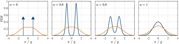
Figure 3: The optimal input and output distributions for the SISO ISAC channel (15). The curves are from Algorithm 1 with $\hbar=1$, $\varepsilon_{\!J}=1{{\mathsf{e}}}-4$, $\varepsilon_{\mu}=1{{\mathsf{e}}}-8$, and analytical results. In this plot, $\sigma_{\mathsf{g}}^{2}=\sigma_{\mathsf{h}}^{2}=1$, and $P_{0}=\sigma_{\rm c}^{2}=\sigma_{\rm s}^{2}=$1\text{\,}\mathrm{W}$$.

Under the formulation of SISO ISAC channel (15), the MMSE-Rate limit-achieving distribution can be numerically obtained based on Algorithm 1, as shown in Fig. 3. As the preference of functionality of the ISAC signal $\mathsf{x}$ moving from sensing ($\alpha=0$) to communication ($\alpha=1$), the optimal input distribution shifts gradually from a binary distribution with equal probability to a pure Gaussian, and the optimal output distribution transients from a Gaussian convolution with a binary distribution, which has heavier tails, to a pure Gaussian. Intuitively, the ISAC signal must carry more randomness, i.e., become more Gaussian-like, in order to convey more information.

III-C Sensing- and Communication-Optimal Points Performance Characterization and Discussion

The performance limit at SAC optimal points are crucial in designing corresponding sensing- and communication-centric ISAC systems, and to gain more insights on the SAC tradeoff within ISAC systems. This paper next presents a detailed investigation on these two points, including the SAC performance and the corresponding achieving-strategy. Lying on the two ends of the MMSE-Rate limit curve characterized by (9), the SAC optimal points $\mathcal{P}_{\rm s}(\epsilon_{\rm s},\mathcal{R}_{\rm s})$ and $\mathcal{P}_{\rm c}(\epsilon_{\rm c},\mathcal{R}_{\rm c})$ are

$$\epsilon_{\rm s} :=\epsilon(0)=\inf_{p_{\bm{\mathsf{X}}}(\bm{X})}\ \mathbb{E}_{\bm{\mathsf{X}}}\left[\Phi\left({\bm{I}}_{N_{\rm{s}}}\otimes\bm{\mathsf{R}}_{\bm{\mathsf{X}}}\right)\right];$$ (20a)

$$\mathcal{R}_{\rm s} :=\mathcal{R}(0)=\sup_{p_{\bm{\mathsf{X}}}(\bm{X})}\ \mathcal{R}\quad\rm{s.t.}\quad\epsilon=\epsilon_{\rm s};$$ (20b)

$$\mathcal{R}_{\rm c} :=\mathcal{R}(1)=\sup_{p_{\bm{\mathsf{X}}}(\bm{X})}\ T^{-1}I(\bm{\mathsf{X}};\bm{\mathsf{Y}}|\bm{\mathsf{H}});$$ (20c)

$$\epsilon_{\rm c} :=\epsilon(1)=\inf_{p_{\bm{\mathsf{X}}}(\bm{X})}\ \epsilon\quad\rm{s.t.}\quad\mathcal{R}=\mathcal{R}_{\rm c}.$$ (20d)

III-C1 Sensing-Optimal Point $\mathcal{P}_{\rm s}$

Aligned with the sensing-centric ISAC design [4] which tries to introduce communication signaling without affecting the sensing performance, the sensing-optimal point $\mathcal{P}_{\rm s}$ characterizes the best communication performance limited by the ISAC sensing-only scenario, where the channel estimation MSE should be minimized. The best sensing performance $\epsilon_{\rm s}$ (20a) is obtained by solving (9) with $\alpha=0$

$$\epsilon_{\rm s}=\inf_{p_{\bm{\mathsf{X}}}(\bm{X})}\quad\mathbb{E}_{\bm{\mathsf{X}}}\left[\Phi\left({\bm{I}}_{N_{\rm{s}}}\otimes\bm{\mathsf{R}}_{\bm{\mathsf{X}}}\right)\right]$$ (21)

$$\rm{s.t.} \bm{\mathsf{R}}_{\bm{\mathsf{X}}}=\bm{\mathsf{R}}_{\bm{\mathsf{X}}}^{\dagger},\ \bm{\mathsf{R}}_{\bm{\mathsf{X}}}\succeq\mathbf{0},\ {{\rm{Tr}}}\left[\mathbb{E}(\bm{\mathsf{R}}_{\bm{\mathsf{X}}})\right]=NP_{0}.$$

Denote $\bm{\mathsf{X}}_{\rm s}$ as the sensing-optimal waveform that achieves $\epsilon_{\rm s}$, and $\bm{X}_{\rm s}$ as its realization. The sensing-limited rate (20b) is

$$\mathcal{R}_{\rm s}=\sup_{p_{\bm{\mathsf{X}}_{\rm s}}(\bm{X}_{\rm s})}\quad T^{-1}I(\bm{\mathsf{X}}_{\rm s};\bm{\mathsf{Y}}|\bm{\mathsf{H}}),$$ (22)

where $p_{\bm{\mathsf{X}}_{\rm s}}(\bm{X}_{\rm s})$ (e.g., $p_{\bm{\mathsf{X}}}^{\star}(\bm{X},1)$) is the solution that optimizes (21).

Based on the definition of $\mathcal{P}_{\rm s}(\epsilon_{\rm s},\mathcal{R}_{\rm s})$, the sensing-optimal waveform structure may be characterized as follows.

Theorem 3

The correlation matrix of sensing-optimal waveform $\bm{\mathsf{X}}_{\rm s}$ is deterministic and unique, namely,

$$\bm{\mathsf{R}}_{\bm{\mathsf{X}}_{\rm s}}=\bm{R}_{\bm{\mathsf{X}}_{\rm s}}.$$ (23)

Proof:

Before diving into specific proof, the following lemma is first presented.

Lemma 1

$\Phi({\bm{I}}_{N_{\rm{s}}}\otimes\bm{R})$ is strictly convex about $\bm{R}$.

Proof:

See convexity of the operator ${\rm{Tr}}[(\cdot)^{-1}]$ in [25, Chapter 3]. ∎∎

According to Lemma 1,

$$\mathbb{E}_{\bm{\mathsf{X}}}\left[\Phi\left({\bm{I}}_{N_{\rm{s}}}\otimes\bm{\mathsf{R}}_{\bm{\mathsf{X}}}\right)\right]\geq\Phi\left[{\bm{I}}_{N_{\rm{s}}}\otimes\mathbb{E}_{\bm{\mathsf{X}}}\left(\bm{\mathsf{R}}_{\bm{\mathsf{X}}}\right)\right].$$ (24)

From (21),

$$\epsilon_{\rm s} =\ \min_{p_{\bm{\mathsf{X}}}(\bm{X})}\quad\mathbb{E}_{\bm{\mathsf{X}}}\left[\Phi\left({\bm{I}}_{N_{\rm{s}}}\otimes\bm{\mathsf{R}}_{\bm{\mathsf{X}}}\right)\right]$$ (25)

$$=\ \min_{p_{\bm{\mathsf{X}}}(\bm{X})}\quad\Phi\left[{\bm{I}}_{N_{\rm{s}}}\otimes\mathbb{E}_{\bm{\mathsf{X}}}\left(\bm{\mathsf{R}}_{\bm{\mathsf{X}}}\right)\right]$$

$$=\ \min_{p_{\bm{\mathsf{X}}}(\bm{X})}\quad\Phi\left({\bm{I}}_{N_{\rm{s}}}\otimes\bm{R}_{\bm{\mathsf{X}}}\right)$$

$$=\ \Phi\left({\bm{I}}_{N_{\rm{s}}}\otimes\bm{R}_{\bm{\mathsf{X}}}\right).$$

The equality in (24) holds if and only if $\bm{\mathsf{R}}_{\bm{\mathsf{X}}}$ is itself deterministic, namely $\bm{\mathsf{R}}_{\bm{\mathsf{X}}}=\mathbb{E}(\bm{\mathsf{R}}_{\bm{\mathsf{X}}})=\bm{R}_{\bm{\mathsf{X}}}$. Therefore, $\epsilon_{\rm s}$ is achieved if and only if the sensing-optimal sample correlation matrix is deterministic. To demonstrate the uniqueness, assume $\bm{R}_{1}$ and $\bm{R}_{2}$ are both sensing-optimal correlation matrices that minimize $\epsilon$ with $\bm{R}_{1}\neq\bm{R}_{2}$. Denote $\tilde{\bm{R}}=(\bm{R}_{1}+\bm{R}_{2})/2$.

$$\Phi({\bm{I}}_{N_{\rm{s}}}\otimes\tilde{\bm{R}})<\frac{1}{2}\Phi({\bm{I}}_{N_{\rm{s}}}\otimes{\bm{R}_{1}})+\frac{1}{2}\Phi({\bm{I}}_{N_{\rm{s}}}\otimes{\bm{R}_{2}})=\epsilon_{\rm s},$$

due to strict convexity. This leads to a contradiction. Therefore, the sensing-optimal correlation matrix is unique. ∎∎

Theorem 3 gives a necessary condition for the sensing-optimal waveform: in order to achieve $\mathcal{P}_{\rm s}$, only signals with a deterministic sample correlation matrix can be transmitted. Indeed, the sensing-optimal waveform still maintains randomness, but due to the constraints on a deterministic sample correlation matrix, its randomness is greatly reduced. This conclusion is a generalization of the sensing-optimal distribution for the SISO case in Theorem 2 and Fig. 3. However, the sensing-optimal waveform and corresponding MMSE performance $\epsilon_{\rm s}$ are hard to derive for now.

Note that ${\bm{\mathsf{g}}}_{i}=\bm{\mathsf{G}}^{\mathsf{T}}\textbf{\em e}_{i}$ is the target response of the $i$-th receive antenna from the transmit antenna array. With widely-distributed sensing receivers, the correlation among the rows of target response matrix $\bm{\mathsf{G}}$ can be neglected [26, 15, 27, 28], and ${\bm{\mathsf{g}}}_{i}$’s are assumed to be i.i.d.. Next, this paper modifies assumption (A1) to (A1*) for further investigation.

1. Sensing Channel with Widely-Distributed Sensing Receivers. $\bm{\mathit{\bar{\Sigma}}}_{\!{\bm{\mathsf{g}}}}$ strictly block-diagonal with all its block matrices identical. The rows of $\bm{\mathsf{G}}$ are independently and identically circular symmetrical complex Gaussian distributed with zero mean. The diagonal covariance matrices are the same for $\bm{\mathsf{G}}$’s each row ${\bm{\mathsf{g}}}_{i}$, namely $\bm{\mathit{{\Sigma}}}_{\!{\bm{\mathsf{g}}}}:=\mathbb{E}[{\bm{\mathsf{g}}}_{i}{\bm{\mathsf{g}}}_{i}^{\dagger}]$ for $i\in\{1,\cdots,N_{\rm{s}}\}$, and $\mathbb{E}({\bm{\mathsf{g}}}_{i}{\bm{\mathsf{g}}}_{j}^{\dagger})=\mathbf{0}$ for any $j\neq i$ due to independence. Therefore, $\bm{\mathit{\bar{\Sigma}}}_{\!{\bm{\mathsf{g}}}}={\bm{I}}_{N_{\rm{s}}}\otimes\bm{\mathit{{\Sigma}}}_{\!{\bm{\mathsf{g}}}}$.

The eigenvalue decomposition of $\bm{\mathit{{\Sigma}}}_{\!{\bm{\mathsf{g}}}}$ is

$$\bm{\mathit{{\Sigma}}}_{\!{\bm{\mathsf{g}}}}={{\bm{\mathit{U}}}_{\!{\bm{\mathsf{g}}}}}{\bm{\mathit{\Lambda}}}_{\bm{\mathsf{g}}}{\bm{\mathit{U}}}_{\!{\bm{\mathsf{g}}}}^{\dagger},$$ (26)

where ${{\bm{\mathit{U}}}_{\!{\bm{\mathsf{g}}}}}$ is a unitary matrix with $\bm{\mathit{{\Sigma}}}_{\!{\bm{\mathsf{g}}}}$’s eigenvectors as its columns, and $\bm{\mathit{\Lambda}}_{\bm{\mathsf{g}}}={\rm diag}(\lambda_{1},\cdots,\lambda_{N})$ stores all non-negative eigenvalues of $\bm{\mathit{{\Sigma}}}_{\!{\bm{\mathsf{g}}}}$ on its diagonal. Based on assumption (A1*), this paper derives the sensing-optimal waveform $\bm{\mathsf{X}}_{\rm s}$ and its corresponding MMSE $\epsilon_{\rm s}$ in the following theorem.

Theorem 4 (Closed-form sensing-optimal waveform and the corresponding MMSE)

When (A1*) holds, $\epsilon_{\rm s}$ can be achieved with the following sensing-optimal waveform

$$\bm{\mathsf{X}}_{\rm s}={\bm{\mathit{U}}}_{\!{\bm{\mathsf{g}}}}\bm{\mathit{P}}_{\!\rm s}^{1/2}\bm{\mathsf{\Psi}},$$ (27)

where ${\bm{\mathsf{\Psi}}}\in\mathbb{C}^{N\times T}$ is any matrix with orthonormal rows, i.e., $\bm{\mathsf{\Psi}}\bm{\mathsf{\Psi}}^{\dagger}={\bm{I}}_{N}$,

$$\bm{\mathit{P}}_{\!\rm s}={\rm diag}\left[\left(\eta_{\rm s}-\frac{\sigma_{\rm s}^{2}}{\lambda_{1}}\right)^{+},\cdots,\left(\eta_{\rm s}-\frac{\sigma_{\rm s}^{2}}{\lambda_{N}}\right)^{+}\right]$$ (28)

is the water-filling power allocation matrix according to $\bm{\mathit{{\Sigma}}}_{\!{\bm{\mathsf{g}}}}$, where $\eta_{\rm s}$ is chosen such that

$$\sum_{i=1}^{N}\left({\eta}_{\rm s}-\frac{\sigma_{\rm s}^{2}}{\lambda_{i}}\right)^{+}=TNP_{0},$$ (29)

and ${{{\bm{\mathit{U}}}_{\!{\bm{\mathsf{g}}}}}}$ is defined in (26). The resulting MMSE is given as

$$\epsilon_{\rm s}=N_{\rm{s}}\sum_{i=1}^{N}\frac{\lambda_{i}}{(\lambda_{i}\sigma_{\rm s}^{-2}\eta_{\rm s}-1)^{+}+1}.$$ (30)

Furthermore, the sensing-optimal correlation matrices are

$$\bm{\mathsf{R}}_{\bm{\mathsf{X}}_{\rm s}}=\bm{R}_{\bm{\mathsf{X}}_{\rm s}}=\frac{1}{T}{\bm{\mathit{U}}}_{\!{\bm{\mathsf{g}}}}\bm{\mathit{P}}_{\!\rm s}{\bm{\mathit{U}}}_{\!{\bm{\mathsf{g}}}}^{\dagger}.$$ (31)

Proof:

See Appendix D. ∎∎

As shown in (27) – (30), the power allocation for the sensing-optimal waveform actually employs the water-filling strategy, which allocates the transmitted power in reverse proportion to the eigenvalue of $\bm{\mathit{{\Sigma}}}_{\!{\bm{\mathsf{g}}}}$. An intuitive understanding is that water-filling focus the signal power in the direction with the presence of significant scattering of the target, and allocates less power in the direction with less prominent target scattering compared with the noise, i.e., where $\sigma_{\rm s}^{2}/\lambda_{i}$ large.

The sensing-optimal waveform’s correlation matrix (31) is unique for a given $\bm{\mathit{\bar{\Sigma}}}_{\!{\bm{\mathsf{g}}}}={\bm{I}}_{N_{\rm{s}}}\otimes\bm{\mathit{{\Sigma}}}_{\!{\bm{\mathsf{g}}}}$. Since ${{\bm{\mathit{U}}}_{\!{\bm{\mathsf{g}}}}}$ and $\bm{\mathit{P}}_{\!\rm s}$ are completely deterministic and determined by the sensing channel statistics, the waveform (27) has randomness only in the semi-unitary matrix $\bm{\mathsf{\Psi}}$ that can be used to convey information. To investigate the best communication performance, i.e., the maximum rate, achieved by the sensing-optimal waveform (27) is typically unprocurable. Thanks to [7, 19], the sensing-limited capacity is proven to be achieved when $\bm{\mathsf{\Psi}}$ is uniformly sampled from the set of all orthonormal matrices, i.e., the complex Stiefel manifold, $\{\bm{\mathsf{\Psi}}\in\mathbb{C}^{N\times T}|\bm{\mathsf{\Psi}}\bm{\mathsf{\Psi}}^{\dagger}={\bf I}_{N}\}$.

Theorem 5 (Sensing-limited high SNR ergodic rate)

When (A1*) holds, in the high SNR region (i.e., when $P_{0}/\sigma_{\rm c}^{2}$ very large), the rate can be expressed as

$$\mathcal{R}_{\rm s}=\mathbb{E}_{\bm{\mathsf{H}}} \left[\left(1-\frac{\mathsf{r}_{\rm s}}{2T}\right)\log\det\left(\frac{\bm{\mathsf{H}}{\bm{\mathit{U}}}_{\!{\bm{\mathsf{g}}}}\bm{\mathit{P}}_{\!\rm s}{\bm{\mathit{U}}}_{\!{\bm{\mathsf{g}}}}^{\dagger}\bm{\mathsf{H}}^{\dagger}}{\sigma_{\rm c}^{2}T}\right)+\mathsf{c}_{0}\right]$$

$$+O(\sigma_{\rm c}^{2}),$$ (32)

where $\mathsf{r}_{\rm s}={\rm{rank}}(\bm{\mathsf{H}}{\bm{\mathit{U}}}_{\!{\bm{\mathsf{g}}}}\bm{\mathit{P}}_{\!\rm s}{\bm{\mathit{U}}}_{\!{\bm{\mathsf{g}}}}^{\dagger}\bm{\mathsf{H}}^{\dagger})$, and

$$\mathsf{c}_{0}=\frac{\mathsf{r}_{\rm s}}{T}\left[\left(T-\frac{\mathsf{r}_{\rm s}}{2}\right)\log\frac{T}{{{\mathsf{e}}}}-\log\Gamma(T)+\log(2\sqrt{\pi})\right],$$

with ${{\mathsf{e}}}=2.718\cdots$ is the Euler’s constant, and $\Gamma(\cdot)$ is the Gamma function.

Proof:

See [19] and [7, Theorem 1] and replace the sensing-optimal statistical correlation matrix with (31). ∎∎

Based on Theorem 4, the best MMSE estimator for the sensing channel that achieves (30) can be derived as

$$\hat{{\bm{\mathsf{g}}}}_{\rm s}={\bm{I}}_{N_{\rm{s}}}\otimes\left[(\sigma_{\rm s}^{2}\bm{\mathit{{\Sigma}}}_{\!{\bm{\mathsf{g}}}}^{-1}+{\bm{\mathit{U}}}_{\!{\bm{\mathsf{g}}}}\bm{\mathit{P}}_{\!\rm s}{\bm{\mathit{U}}}_{\!{\bm{\mathsf{g}}}}^{\dagger})^{\!-1}{\bm{\mathit{U}}}_{\!{\bm{\mathsf{g}}}}\bm{\mathit{P}}_{\!\rm s}^{1/2}\bm{\mathsf{\Psi}}\right]{\bm{\mathsf{s}}}.$$ (33)

III-C2 Communication-Optimal Point $\mathcal{P}_{\rm c}$

Aligned with the communication-centric ISAC design [4] which tries to extract sensing information based on communication setups, the communication-optimal point $\mathcal{P}_{\rm c}$ characterizes the best sensing performance limited by the ISAC communication-only scenario, where the rate should be maximized. The best communication performance $\mathcal{R}_{\rm c}$ (20c) is obtained by solving the following optimization problem

$$\mathcal{R}_{\rm c}= \sup_{p_{\bm{\mathsf{X}}}(\bm{X})}\quad T^{-1}{I(\bm{\mathsf{X}};\bm{\mathsf{Y}}|\bm{\mathsf{H}})}$$ (34)

$$\rm{s.t.} \bm{R}_{\bm{\mathsf{X}}}=\bm{R}_{\bm{\mathsf{X}}}^{\dagger},\ \bm{R}_{\bm{\mathsf{X}}}\succeq\mathbf{0},\ {{\rm{Tr}}}(\bm{R}_{\bm{\mathsf{X}}})=NP_{0}.$$

Denote $\bm{\mathsf{X}}_{\rm c}$ as the communication-optimal waveform that maximizes $\mathcal{R}$, and $\bm{X}_{\rm c}$ as its realization. The communication-limited MMSE is defined as

$$\epsilon_{\rm c}=\mathbb{E}_{\bm{\mathsf{H}}}\left\{\inf_{p_{\bm{\mathsf{X}}_{\rm c}}(\bm{X}_{\rm c})}\quad\mathbb{E}_{\bm{\mathsf{X}}_{\rm c}}\left[\Phi\left({\bm{I}}_{N_{\rm{s}}}\otimes\bm{\mathsf{R}}_{\bm{\mathsf{X}}_{\rm c}}\right)\right]\right\},$$ (35)

where $p_{\bm{\mathsf{X}}_{\rm c}}(\bm{X}_{\rm c})$ is limited to the optimal distribution that optimizes (34), and $\bm{\mathsf{R}}_{\bm{\mathsf{X}}_{\rm c}}$ is the communication-optimal signal’s sample correlation matrix. Unlike the sensing-optimal case that still has degree of freedom in the distribution of the semi-unitary matrix $\bm{\mathsf{\Psi}}$ to convey information, the $\mathcal{P}_{\rm c}-$achieving distribution $p_{\bm{\mathsf{X}}_{\rm c}}(\bm{X}_{\rm c})$ is completely determined by the given communication channel realization in each block, as seen in the next theorem. Therefore, there is no further DoF to optimize the communication-limited sensing performance. As a result, (20d) reduces to

$$\epsilon_{\rm c}=\mathbb{E}\left[\Phi\left({\bm{I}}_{N_{\rm{s}}}\otimes\bm{\mathsf{R}}_{\bm{\mathsf{X}}_{\rm c}}\right)\right],$$ (36)

where the expectation is taken with respect to both $\bm{\mathsf{X}}_{\rm c}$ and $\bm{\mathsf{H}}$.

Theorem 6 (Closed-form communication-optimal waveform and the corresponding maximum ergodic rate)

For a given channel realization $\bm{H}$ in each block, the communication-optimal waveform $\bm{\mathsf{X}}_{\rm c}$ that maximizes the rate is distributed in the way such that each column of $\bm{\mathsf{X}}_{\rm c}$ follows i.i.d. zero mean circular symmetrical complex Gaussian distribution with statistical covariance matrix

$$\bm{R}_{\bm{\mathsf{X}}_{\rm c}}={\bm{\mathit{U}}}_{\!\!\bm{H}}\bm{\mathit{P}}_{\!\rm c}\!{\bm{\mathit{U}}}_{\!\!\bm{H}}^{\dagger},$$ (37)

i.e.,

$$\bm{\mathsf{X}}_{\rm c}={\bm{\mathit{U}}}_{\!\!\bm{H}}\bm{\mathit{P}}_{\!\rm c}^{1/2}\bm{\mathsf{N}},$$ (38)

where ${\bm{\mathit{U}}}_{\!\!\bm{H}}\in\mathbb{C}^{N_{\rm{c}}\times r_{\!\bm{H}}}$ is from the decomposition $\bm{H}^{\dagger}\bm{H}={\bm{\mathit{U}}}_{\!\bm{H}}\bm{\mathit{\Gamma}}_{\!\bm{H}}\!{\bm{\mathit{U}}}_{\!\!\bm{H}}^{\dagger}$, $r_{\bm{H}}={\rm{rank}}(\bm{H})$,

$$\bm{\mathit{P}}_{\!\rm c}={\rm diag}\left[\left(\eta_{\rm c}-\frac{\sigma_{\rm c}^{2}}{\gamma_{1}}\right)^{+},\cdots,\left(\eta_{\rm c}-\frac{\sigma_{\rm c}^{2}}{\gamma_{r_{\bm{H}}}}\right)^{+}\right],$$ (39)

$\gamma_{i}$ is the $i$-th diagonal entry of $\bm{\mathit{\Gamma}}_{\!\bm{H}}$, i.e., $\gamma_{i}=[\bm{\mathit{\Gamma}}_{\!\bm{H}}]_{ii}$, $\eta_{\rm c}$ is chosen such that

$$\sum_{i=1}^{r_{\bm{H}}}\left(\eta_{\rm c}-\frac{\sigma_{\rm c}^{2}}{\gamma_{i}}\right)^{+}=NP_{0},$$ (40)

and $\bm{\mathsf{N}}\in\mathbb{C}^{r_{\!\bm{H}}\times T}$ has i.i.d. zero-mean circular symmetrical complex Gaussian entries with unit variance, i.e., $\mathbb{E}(\bm{\mathsf{N}}\bm{\mathsf{N}}^{\dagger})=T{\bm{I}}_{r_{\bm{H}}}$. The resulted coherent rate for the particular channel realization $\bm{H}$ is $\sum_{i=1}^{r_{\!\bm{H}}}[\log(\sigma_{\rm c}^{-2}\eta_{\rm c}\gamma_{i})]^{+}$.

The ergodic coherent rate at $\mathcal{P}_{\rm c}$ is

$$\mathcal{R}_{\rm c}=\ \mathbb{E}_{\bm{\mathsf{H}}}\left[\sum_{i=1}^{r_{\bm{\mathsf{H}}}}[\log(\sigma_{\rm c}^{-2}\eta_{\rm c}\gamma_{i})]^{+}\right].$$ (41)

Proof:

See Appendix E. ∎∎

In the next part, this paper presents discussions on the derived analytical results in previous sections for a better understanding of the MMSE-Rate limit and its achieving strategies.

III-C3 Tradeoffs between Sensing and Communication

Reviewing the limit-achieving conditions (Section LABEL:sec:results_limit) and structure of closed-form SAC-optimal waveforms (Section III-C) derived so far, this paper highlights presence of two tradeoffs between sensing and communication, as summarized below.

Water-Filling Tradeoff

To achieve $\mathcal{P}_{\rm s}$, the signal power is spatially allocated in the direction with the presence of significant scattering of the indicated by matrix $\bm{\mathit{P}}_{\!\rm s}$, according to the a priori knowledge of sensing channel statistics, i.e. $\bm{\mathit{\bar{\Sigma}}}_{\!{\bm{\mathsf{g}}}}$. To achieve $\mathcal{P}_{\rm c}$, the signal power is spatially allocated to the “strongest” communication sub-channels (those with high SNRs) indicated by matrix $\bm{\mathit{P}}_{\!\rm c}$, according to full communication CSI knowledge $\bm{H}$ at the transmitter. Indeed, the total ISAC signal power is shared between sensing and communication, but it’s not possible to simultaneously achieve the optimal water-fillings for both sensing and communication. Thus, a water-filling tradeoff naturally exists, which can be controlled by allocating the power of the transmitted signal more “aligned” in favor of either the sensing or communication channel.

Waveform Uncertainty Tradeoff

Reviewing the tendency of change of randomness of the input distribution along the performance limit curve (Fig. 3), the input signal is becoming more predictable from $\alpha=1$ to $0$. As extreme cases, at the communication-optimal point $\mathcal{P}_{\rm c}$, the Gaussian waveform $\bm{\mathsf{N}}$ with the largest randomness should be selected; at the sensing-optimal point $\mathcal{P}_{\rm s}$, the isometry waveform $\bm{\mathsf{\Psi}}$ is used, with much-reduced randomness compared with Gaussian.

Intuitively, it is ideal to employ predictable and optimized waveforms for sensing [30]. A deterministic waveform, however, is incapable of carrying any information. Consequently, the ISAC system favors waveform with randomness/uncertainty for carrying information, possibly with a degradation of sensing performance. Regarding this, this paper concludes the waveform uncertainty tradeoff between sensing and communication, which can be controlled by transmitted waveform selection (e.g., Gaussian, isometry, or any other random waveforms with certain distribution, e.g., in Fig. 3). This conclusion is consistent with those from many ISAC studies [7, 20, 31, 30], although their SAC metrics diverge.

III-C4 Loose Bounds Connecting $\mathcal{P}_{\rm s}$ and $\mathcal{P}_{\rm c}$

The evaluation of the MMSE-Rate performance limit-achieving distribution based on Algorithm 1 is computationally intensive, which involves updating the PDF of several random matrices in the high dimensional complex domain. For fast evaluation of the MMSE-Rate limit, loose bounds may be obtained by leveraging the above-mentioned two tradeoffs. While some bounds in this part are derived in [7, 6, 5], this paper puts them into a unified framework, offers more intuitions, and corrects some of the achieving-strategies.

MMSE-Rate Outer Bound

Due to the complexity of numerically evaluating the MMSE-Rate limit (9), a relaxed version of (9) may be obtained. For any given communication channel realization $\bm{H}$, the following inequalities hold

$$T^{-1}I(\bm{\mathsf{X}};\bm{\mathsf{Y}}|\bm{\mathsf{H}}=\bm{H})\leq\log\det\left({\bm{I}}+\frac{\bm{H}\bm{R}_{\bm{\mathsf{X}}}\bm{H}^{\dagger}}{\sigma_{\rm c}^{2}}\right);$$ (42a)

$$\mathbb{E}_{\bm{\mathsf{X}}}\left[\Phi\left({\bm{I}}_{N_{\rm{s}}}\otimes\bm{\mathsf{R}}_{\bm{\mathsf{X}}}\right)\right]\geq\Phi\left({\bm{I}}_{N_{\rm{s}}}\otimes\bm{R}_{\bm{\mathsf{X}}}\right),$$ (42b)

a natural loose (outer) bound can be obtained [5, 6, 7] from the following optimization problem

$$\sup_{\bm{R}_{\bm{\mathsf{X}}}} \alpha\log\det\left({\bm{I}}+\frac{\bm{H}\bm{R}_{\bm{\mathsf{X}}}\bm{H}^{\dagger}}{\sigma_{\rm c}^{2}}\right)-(1-\alpha)\Phi\left({\bm{I}}_{N_{\rm{s}}}\otimes\bm{R}_{\bm{\mathsf{X}}}\right)$$ (43)

$$\rm{s.t.} \bm{R}_{\bm{\mathsf{X}}}=\bm{R}_{\bm{\mathsf{X}}}^{\dagger},\ \bm{R}_{\bm{\mathsf{X}}}\succeq\mathbf{0},\ {{\rm{Tr}}}(\bm{R}_{\bm{\mathsf{X}}})=NP_{0}.$$

For any given $\alpha\in[0,1]$ and channel realization $\bm{H}$, denote the optimal statistical correlation matrix to (43) as $\bm{R}_{\bm{\mathsf{X}}}^{\star}(\alpha)$, an outer bound $\{(\epsilon^{\rm out}(\alpha),\mathcal{R}^{\rm out}(\alpha))|\alpha\in[0,1]\}$ is given by

$$\mathcal{R}^{\rm out}(\alpha) =\mathbb{E}_{\bm{\mathsf{H}}}\left[\log\det\left({\bm{I}}+\frac{\bm{\mathsf{H}}\bm{R}_{\bm{\mathsf{X}}}^{\star}(\alpha)\bm{\mathsf{H}}^{\dagger}}{\sigma_{\rm c}^{2}}\right)\right];$$ (44a)

$$\epsilon^{\rm out}(\alpha) =\mathbb{E}\left\{\Phi\left[{\bm{I}}\otimes\bm{R}_{\bm{\mathsf{X}}}^{\star}(\alpha)\right]\right\}.$$ (44b)

(44) is achieved when the input signal $\bm{\mathsf{X}}$ is simultaneously Gaussian (for the equality in (44a) to hold) and isometry (for the equality in (44b) to hold), which is not practically feasible. As a result, (44) is an outer bound.

MMSE-Rate Inner Bounds

Based on the MMSE-Rate outer bound (44), the following achievable inner bounds may be obtained with the following signaling strategies.

1. “$\mathcal{P}_{\rm s}-\mathcal{P}_{\rm c}$ Time-Sharing” Bound. The two optimal points $\mathcal{P}_{\rm s}$ and $\mathcal{P}_{\rm c}$ maybe connected exploiting the time-sharing strategy, which assigns probability $p_{\rm s}\in[0,1]$ to apply the $\mathcal{P}_{\rm s}-$achieving strategy and probability $p_{\rm c}=1-p_{\rm s}$ to apply the $\mathcal{P}_{\rm c}-$achieving strategy [7]. This is a baseline ISAC scheme which splits orthogonal resources between sensing and communication [20] due to the inability to simultaneously perform SAC functionalities.

2. “Sensing-Based Inner Bound”. Motivated by the $\mathcal{P}_{\rm s}-$achieving strategy, a sensing-based inner bound (SIB) $\{(\mathcal{R}^{\rm in}_{\rm s}(\alpha),\epsilon^{\rm in}_{\rm s}(\alpha))|\alpha\in[0,1]\}$ can be achieved by transmitting the following isometry signal

   $${\bm{\mathsf{X}}^{\rm in}_{\rm s}(\alpha)=\sqrt{T}{\bm{\mathit{U}}}_{\!\alpha}{\bm{\mathit{\Omega}}}_{\alpha}^{1/2}\bm{\mathsf{\Psi}}_{\alpha}}$$ (45)

   for each $\alpha\in[0,1]$, where ${\bm{\mathit{U}}}_{\!\alpha}\in\mathbb{C}^{N\times r_{\alpha}}$ and ${\bm{\mathit{\Omega}}}_{\alpha}\in\mathbb{R}^{r_{\alpha}\times r_{\alpha}}$ are from the decomposition of $\bm{R}_{\bm{\mathsf{X}}}^{\star}(\alpha)$, i.e.,

   $$\bm{R}_{\bm{\mathsf{X}}}^{\star}(\alpha)={\bm{\mathit{U}}}_{\!\alpha}{\bm{\mathit{\Omega}}}_{\alpha}{\bm{\mathit{U}}}_{\!\alpha}^{\dagger},$$ (46)

   $r_{\alpha}={\rm{rank}}[\bm{R}_{\bm{\mathsf{X}}}^{\star}(\alpha)]$, and $\bm{\mathsf{\Psi}}_{\alpha}\in\mathbb{C}^{r_{\alpha}\times T}$ is a random matrix with orthonormal rows uniformly sampled from the complex Stiefel manifold $\{{\bm{\mathsf{\Psi}}_{\alpha}}\in\mathbb{C}^{r_{\alpha}\times T}|{\bm{\mathsf{\Psi}}_{\alpha}\bm{\mathsf{\Psi}}_{\alpha}^{\dagger}}={{\bm{I}}}_{r_{\alpha}}\}$. The corresponding hish-SNR bound is

   $$\mathcal{R}^{\rm in}_{\rm s}(\alpha)= \ \mathbb{E}_{\bm{\mathsf{H}}}\left[\left(1-\frac{\mathsf{r}_{\bm{\mathsf{H}}\alpha}}{2T}\right)\log\left|\frac{\bm{\mathsf{H}}\bm{R}_{\bm{\mathsf{X}}}^{\star}(\alpha)\bm{\mathsf{H}}^{\dagger}}{\sigma_{\rm c}^{2}}\right|\!\!+\!\mathsf{c}_{0}^{\alpha}\right]$$

   $$+O(\sigma_{\rm c}^{2});$$ (47a)

   $$\epsilon^{\rm in}_{\rm s}(\alpha)= \ \epsilon^{\rm out}(\alpha),$$ (47b)

   where $\mathsf{r}_{\bm{\mathsf{H}}\alpha}={\rm{rank}}(\bm{\mathsf{H}}\bm{R}_{\bm{\mathsf{X}}}^{\star}(\alpha)\bm{\mathsf{H}}^{\dagger})$, and

   $$\mathsf{c}_{0}^{\alpha}=\frac{\mathsf{r}_{\bm{\mathsf{H}}\alpha}}{T}\left[\left(T-\frac{\mathsf{r}_{\bm{\mathsf{H}}\alpha}}{2}\right)\log\frac{T}{{{\mathsf{e}}}}-\log\Gamma(T)+\log(2\sqrt{\pi})\right].$$

3. “Communication-Based Inner Bound”. Motivated by the $\mathcal{P}_{\rm c}-$achieving strategy, a communication-based inner bound (CIB) $\{(\mathcal{R}^{\rm in}_{\rm c}(\alpha),\epsilon^{\rm in}_{\rm c}(\alpha))|\alpha\in[0,1]\}$ can be achieved by transmitting the following Gaussian signal

   $$\bm{\mathsf{X}}^{\rm in}_{\rm c}(\alpha)={\bm{\mathit{U}}}_{\!\alpha}\bm{\mathit{\Omega}}_{\alpha}^{1/2}\bm{\mathsf{N}}_{\alpha},$$ (48)

   where ${\bm{\mathit{U}}}_{\!\alpha}$ and $\bm{\mathit{\Omega}}_{\alpha}$ are from (46), and $\bm{\mathsf{N}}_{\alpha}\in\mathbb{C}^{r_{\alpha}\times N}$ has i.i.d. zero-mean circular symmetrical complex Gaussian entries with unit variance, i.e., $\mathbb{E}(\bm{\mathsf{N}}_{\alpha}\bm{\mathsf{N}}_{\alpha}^{\dagger})=T{\bm{I}}_{r_{\alpha}}$. The bound is

   $$\mathcal{R}^{\rm in}_{\rm c}(\alpha) =\mathcal{R}^{\rm out}(\alpha);$$ (49a)

   $$\epsilon^{\rm in}_{\rm c}(\alpha) =\mathbb{E}\left\{{\Phi}\left[{\bm{I}}\otimes\bm{\mathsf{R}}_{\bm{\mathsf{X}}}^{\star}(\alpha)\right]\right\},$$ (49b)

   where $\bm{\mathsf{R}}_{\bm{\mathsf{X}}}^{\star}(\alpha)$ is the sample correlation matrix according to the communication-optimal distribution $\mathcal{CN}(\mathbf{0},\bm{R}_{\bm{\mathsf{X}}}^{\star}(\alpha))$.

4. “CIB-SIB Time-Sharing” Bound. A time-sharing inner bound between the CIB and SIB (with respective probability $p_{\rm c}$ to apply the CIB achieving strategy and $p_{\rm s}=1-p_{\rm c}$ to apply the SIB achieving strategy) can be obtained, which is the convex envelope of CIB and SIB.

Note that when $T$ is very large, $\bm{\mathsf{R}}_{\bm{\mathsf{X}}}\approx\bm{R}_{\bm{\mathsf{X}}}$, i.e., the sample correlation matrix is convergent to the statistical correlation matrix. If $\bm{\mathsf{X}}(\alpha)=\bm{\mathsf{X}}^{\rm in}_{\rm c}(\alpha)$ is transmitted, both equalities in (42) asymptotically hold. Therefore, this outer bound can be asymptotically achieved when each column of $\bm{\mathsf{X}}(\alpha)$ follows the i.i.d. $\mathcal{CN}(\mathbf{0},\bm{R}_{\bm{\mathsf{X}}}^{\star}(\alpha))$ when $T$ is large. Reviewing this, the waveform uncertainty tradeoff becomes less important, and water-filling tradeoff flexibly adjusts the system’s ISAC performance when the coherence time $T$ is large.

III-D Signaling Strategy for Coincided Sensing and Communication Channel

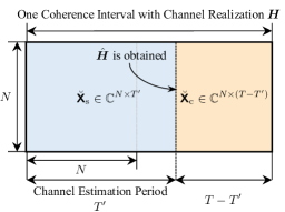
Figure 4: ISAC signaling strategy for the case of coincided SAC channel.

As is often the case, sensing and communication channels can be coincided, i.e., $\bm{\mathsf{G}}=\bm{\mathsf{H}}$. To make follow-up discussions fully applicable, assumptions in Section II should be modifed accordingly as follows. $\bm{\mathsf{G}}$ has the same distribution with $\bm{\mathsf{H}}$, and $\bm{\mathit{\bar{\Sigma}}}_{\!{\bm{\mathsf{g}}}}=\sigma_{\mathsf{h}}^{2}{\bm{I}}_{NN_{\rm{c}}}$, and the full CSI of every $\bm{H}$ is unavailable at the transmitter.

When the Tx does not know the CSI, the “capacity” (i.e., the non-coherent capacity [19]) is achieved by transmitting a Gaussian signal $\ddot{\bm{\mathsf{X}}}_{\rm c}$ with equal power allocation in each transmit antenna [18, Section 10.3], i.e.,

$$\ddot{\bm{\mathsf{X}}}_{\rm c}=\sqrt{P_{0}}\ddot{\bm{\mathsf{N}}},$$ (50)

and $\bm{R}_{\ddot{\bm{\mathsf{X}}}_{\rm c}}=\mathbb{E}(\frac{1}{T}\ddot{\bm{\mathsf{X}}}_{\rm c}\ddot{\bm{\mathsf{X}}}_{\rm c}^{\dagger})=P_{0}{\bm{I}}_{N}$, where $\ddot{\bm{\mathsf{N}}}\in\mathbb{C}^{N\times T}$ has i.i.d. zero-mean circular symmetrical complex Gaussian entries with unit variance. As a result, with no available CSI at the transmitter, the “maximum rate” (non-coherent capacity) is

$$\ddot{\mathcal{R}}_{\rm c}=\mathbb{E}_{\bm{\mathsf{H}}}\left[\log\det\left({\bm{I}}+\frac{P_{0}}{\sigma_{\rm c}^{2}}\bm{\mathsf{H}}\bm{\mathsf{H}}^{\dagger}\right)\right],$$ (51)

and the corresponding sensing performance limited by $\ddot{\mathcal{R}}_{\rm c}$ is

$$\ddot{\epsilon}_{\rm c}=\mathbb{E}_{\ddot{\bm{\mathsf{X}}}_{\rm c}}\left[\Phi\left({\bm{I}}_{N_{\rm{s}}}\otimes\bm{\mathsf{R}}_{\ddot{\bm{\mathsf{X}}}_{\rm c}}\right)\right],$$ (52)

where $\bm{\mathsf{R}}_{\ddot{\bm{\mathsf{X}}}_{\rm c}}=\frac{1}{T}\ddot{\bm{\mathsf{X}}}_{\rm c}\ddot{\bm{\mathsf{X}}}_{\rm c}^{\dagger}$ is the sample correlation matrix of $\ddot{\bm{\mathsf{X}}}_{\rm c}$.

In [14], it is proven that the non-coherent capacity (51) approaches to the coherent capacity (41) only if $T\to\infty$. Therefore, the waveform (50) suffers from degraded communication performance due to unavailable channel information in general cases with a finite channel coherence time.

Thanks to the sensing capability of an ISAC signal, the CSI can be firstly estimated by it, then the optimal communication waveform can be used to maximize the rate according to the estimated CSI within one coherence interval. This maybe done by using the compound ISAC signal $\breve{\bm{\mathsf{X}}}=[\breve{\bm{\mathsf{X}}}_{\rm s},\breve{\bm{\mathsf{X}}}_{\rm c}]$, where $\breve{\bm{\mathsf{X}}}_{\rm s}\in\mathbb{C}^{N\times T^{\prime}}$ is the sensing-optimal waveform to get the channel estimation result $\hat{\bm{H}}$, and the $\breve{\bm{\mathsf{X}}}_{\rm c}\in\mathbb{C}^{N\times(T-T^{\prime})}$ is the communication-optimal waveform according to the channel estimate $\hat{\bm{H}}$. This is demonstrated in Fig. 4. In such a configuration, $\breve{\bm{\mathsf{X}}}_{\rm s}$ and $\breve{\bm{\mathsf{X}}}_{\rm c}$ can be interpreted as the respective pilot and data signal in conventional communication systems. To correctly estimate the channel, $T^{\prime}\in[N,T]$, where $T^{\prime}$ is the length of the channel estimation period. Intuitively, larger $T^{\prime}$ yields better channel estimation performance (i.e., $\hat{\bm{H}}$ is more accurate).

More specifically on the compound ISAC signal, $\breve{\bm{\mathsf{X}}}_{\rm s}$ is obtained with (27) – (30) with $T$ replaced by $T^{\prime}$, i.e., $\breve{\bm{\mathsf{X}}}_{\rm s}$ occupies first $T^{\prime}$ slots in one coherence interval. The channel estimation results $\hat{\bm{h}}=\hat{\bm{g}}$ can be obtained using (33), where $\hat{\bm{h}}={\rm vec}(\hat{\bm{H}})$. Once $\hat{\bm{H}}$ is obtained, the optimal communication signal (optimal with respect to $\hat{\bm{H}}$) is utilized for more effective data communication, and $\breve{\bm{\mathsf{X}}}_{\rm c}$ is obtained through (38) – (40) with $\bm{H}$ replaced by $\hat{\bm{H}}$ and $T$ replaced by $T-T^{\prime}$. The sensing and communication performance of the compound signal $\breve{\bm{\mathsf{X}}}$ are defined as

$$\breve{\epsilon}:= \breve{\epsilon}_{\rm s}(\breve{\bm{\mathsf{X}}}_{\rm s});$$ (53)

$$\breve{\mathcal{R}}:= \frac{T^{\prime}}{T}\breve{\mathcal{R}}_{\rm s}(\breve{\bm{\mathsf{X}}}_{\rm s})+\frac{T-T^{\prime}}{T}\breve{\mathcal{R}}_{\rm c}(\breve{\bm{\mathsf{X}}}_{\rm c}),$$

where $\breve{\epsilon}_{\rm s}(\breve{\bm{\mathsf{X}}}_{\rm s})$ is the MMSE performance of the signal $\breve{\bm{\mathsf{X}}}_{\rm s}$, which can be evaluated using the similar way as (30); $\breve{\mathcal{R}}_{\rm s}(\breve{\bm{\mathsf{X}}}_{\rm s})$ and $\breve{\mathcal{R}}_{\rm c}(\breve{\bm{\mathsf{X}}}_{\rm c})$ are the rate performance of the signal $\breve{\bm{\mathsf{X}}}_{\rm s}$ and $\breve{\bm{\mathsf{X}}}_{\rm c}$, they can be evaluated using the similar way as (32) and (41), respectively.

IV Numerical Results

In this section, numerical examples are presented to illustrate the derived theories about the ISAC MMSE-Rate characterization.

TABLE I: Numerical Parameter Default Settings

Parameter	Symbol	Value/Range
B-A Tolerance for Lagrange Multiplier	$\varepsilon_{\mu}$	$10^{-8}$
B-A Tolerance for Performance	$\varepsilon_{\!J}$	$10^{-4}$
Comm. Channel Variance	$\sigma_{\mathsf{h}}^{2}$	$1$
Comm. Noise Variance	$\sigma_{\rm c}^{2}$	$1\text{\,}\mathrm{W}$
Sensing Noise Variance	$\sigma_{\rm s}^{2}$	$1\text{\,}\mathrm{W}$
Transmit Power	$NP_{0}$	$15\sim$20\text{\,}\mathrm{d}\mathrm{B}$$

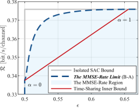
Figure 5: The MMSE-Rate performance limit for fast-fading SISO ISAC channels (15). In this plot, $\sigma_{\mathsf{g}}^{2}=1$, and $P_{0}=$1\text{\,}\mathrm{W}$$.

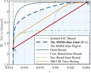
Figure 6: The MMSE-Rate limit and other loose bounds for MIMO ISAC channels.

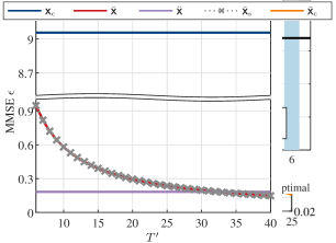
Figure 7: Sensing- and communication-optimal power allocation ($T=1$).

IV-A Setup

The default parameter settings for the numerical plot are summarized in Table I unless otherwise stated. The transmit power is defined as $10\log_{10}(NP_{0})$ in $\text{\,}\mathrm{d}\mathrm{B}\mathrm{W}$, representing the average power of transmit array from the ISAC base station. The numerical results are obtained in MATLAB, where the numerical optimization problems are solved using the numerical optimizer CVX [32], and the expectation operation is conducted with averaging over $10,000$ independent realizations.

IV-B Results

Figure 8: Effects of transmit SNR.

IV-B1 The MMSE-Rate Limit for SISO ISAC channel

This paper first demonstrates the MMSE-Rate limit for SISO ISAC channel as discussed in Section III-A1, i.e., when $N=N_{\rm{c}}=N_{\rm{s}}=1$, and $T=1$. The results are presented in Fig. 5. The limit curve is from the proposed B-A-type algorithm. Note that Fig. 3 portraits the optimal distribution along the limit curve for a particular channel realization $\hbar=1$, while in Fig. 5 the presented results are ergodic, i.e., the performance is averaged according to the channel distribution $\mathsf{h}\sim\mathcal{N}(0,\sigma_{\mathsf{h}}^{2})$. The limit curve exhibits a convex shape with the simply time-sharing between the sensing- and communication- optimal points, as expected.

IV-B2 The MIMO MMSE-Rate Performance Region Characterization

In this part, the sensing channel ${\bm{\mathsf{g}}}$, whose response is very weak due to reflections and longer propagation distances, is configured to have a statistical correlation matrix such that ${\rm{Tr}}({\bm{\mathit{\bar{\Sigma}}}_{\!{\bm{\mathsf{g}}}}})/(NN_{\rm{s}})=0.03.$ In calculation of sensing-limited rate in high-SNR regime, the residual term $O(\sigma_{\rm c}^{2})$ is neglected in (32) and (47), as indicated in [7].

This paper first considers the case where $N=N_{\rm{c}}=N_{\rm{s}}=2$, and $T=2$. Such parameter setting is designed to ensure the numerical feasibility of expectation computations over the PDF of the random matrix, which necessitates a reasonable dimensionality, as suggested in [33]. The MMSE-Rate performance region is characterized in Fig. 6. It is observed both outer bound and SIB-CIB time sharing bound fail to accurately characterize the true limit. Note that the CIB-SIB Time-Sharing bound expects better performance compared with $\mathcal{P}_{\rm s}-\mathcal{P}_{\rm c}$ Time-Sharing, which allocates orthogonal resources between sensing and communication. Still, it fails to fully leverage the WUT by only considering the combination of SAC optimal distributions.

Next, this paper considers $N=6$, $N_{\rm{c}}=N_{\rm{s}}=3$, and $T=6$, i.e., a MIMO ISAC system with larger dimensionality, to study the effects of specific parameter. The optimal power allocation at $\mathcal{P}_{\rm s}$ and $\mathcal{P}_{\rm c}$ is demonstrated in Fig. 7, where the strategy of water-filling is adopted by both sensing and communication. The plot exhibits the water-filling tradeoff. Optimal water-filling at $\mathcal{P}_{\rm s}$ allocates the power to $5$ spatial directions with larger strength of target scatterings, while optimal water-filling at $\mathcal{P}_{\rm c}$ allocates the power to the $3$ strongest sub-channels. Here, the communication degree of freedom is $\min\{N,N_{\rm{c}}\}=N_{\rm{c}}=3$, indicating only a maximal number of $3$ sub-channels can be used to communicate.

The effects of transmit SNR are demonstrated in Fig. 8. With increased SNR, SAC performance gets better. Both $\mathcal{R}_{\rm c}$ and $\epsilon_{\rm s}$ are linear with respect to SNR in $\text{\,}\mathrm{d}\mathrm{B}$, as expected. It is also observed that the performance gaps $\mathcal{R}_{\rm c}-\mathcal{R}_{\rm s}$ and $\epsilon_{\rm c}-\epsilon_{\rm s}$ are increasing with high SNR. One possible reason is that at high SNR, the two optimal power allocation schemes $\bm{\mathit{P}}_{\!\rm s}$ and $\bm{\mathit{P}}_{\!\rm c}$ lose their similarity. E.g., $\bm{\mathit{P}}_{\!\rm s}$ can be quite similar to $\bm{\mathit{P}}_{\!\rm c}$ with some low SNR, i.e., if $\eta_{\rm s}=$200\text{\,}\mathrm{W}$$, only $3$ sensing sub-channels will be allocated power, as seen in Fig. 7; but $\bm{\mathit{P}}_{\!\rm s}$ converges to some scaled version of identity matrix with high SNR, i.e., when $\eta_{\rm s}\to\infty$. Therefore in the high SNR regime, the WFT will become more prominent and restrict $\mathcal{R}_{\rm s}$ and $\epsilon_{\rm c}$.

Figure 9: Effects of sensing channel dimensionality (number of widely-distributed sensing receivers) $N_{\rm{s}}$.

The effects of dimensionality of the sensing channel are demonstrated in Fig. 9, where the normalized MMSE is the MMSE normalized by the size of the sensing channel. The normalized MMSE is used to guarantee a meaningful comparison of the sensing performance when the dimensionalities of the parameters to be estimated are different. With more widely-separated sensing receivers, more independently observed data will be obtained. Therefore, the integration gain is witnessed, and the parameter estimation performance is therefore improved, as indicated in [21]. This result is also aligned with the conclusion in [34].

IV-B3 ISAC Performance with Coincided Sensing and Communication Channel

Figure 10: Communication and sensing performance for different signaling strategies for coincided SAC channel ($T=40$ and $P_{0}=$3\text{\,}\mathrm{W}$$).

Following configuration presented in Section III-D, the results are portrayed in Fig. 10. With longer channel estimation period $T^{\prime}$, both sensing and communication performance of the sensing-optimal waveform $\breve{\bm{\mathsf{X}}}_{\rm s}$ improves, resulting in better channel estimation performance, thus larger rate achieved by the communication optimal waveform $\breve{\bm{\mathsf{X}}}_{\rm c}$. However, larger $T^{\prime}$ does not improve the overall rate $\breve{\mathcal{R}}$, as the overhead is larger (although $\breve{\bm{\mathsf{X}}}_{\rm s}$ indeed provides certain rate). The channel estimation accuracy is good enough for $\breve{\mathcal{R}}_{\rm c}(\breve{\bm{\mathsf{X}}}_{\rm c})$ converge to the coherent rate when $T^{\prime}=N=6$. As a conclusion, for an ISAC system with stronger sensing ability, using the sensing-optimal waveform for channel estimation in a short period of time can achieve better communication performance than non-coherent strategy. This highlights the huge gain of integrating SAC.

An interesting observation is that the sensing performance of the non-coherent communication-optimal signal $\ddot{\bm{\mathsf{X}}}$ is close to the sensing-optimal one. A reasonable explanation is that $T=40$ is large, thus the sample correlation matrix of $\ddot{\bm{\mathsf{X}}}$ is convergent to its statistical one, demonstrating a tendency to behave like the sensing-optimal waveform.

V Conclusion

This paper has provided a systematic framework for identifying the fundamental performance limits of ISAC systems. Using variational calculus, the optimal distributions on the MMSE-Rate limit were investigated, which are solutions to a high-dimensional complex convolutional equation. A Blahut-Arimoto-type algorithm was proposed to numerically evaluate SAC performance and limit-achieving distribution. SAC-optimal closed-form waveforms were derived, which demonstrate the waveform uncertainty tradeoff and waterfilling tradeoff within ISAC. Moreover, a compound signaling strategy for coincided SAC channels was proposed to estimate the channel using the sensing-optimal waveform and to convey information using the communication-optimal waveform over the estimated channel. It demonstrates the potential for significant performance improvements by integrating sensing and communication.

Overall, this study presents an approach to identify the joint estimation- and information-theoretic performance limits for ISAC systems. The theoretical findings in this work highlight both gains and tradeoffs between sensing and communication within an integrated random waveform, and hopefully provide valuable insights into practical ISAC system performance characterization and design for future wireless networks.

Appendix A Proof of Theorem 1

With communication channel realization $\bm{\mathsf{H}}=\bm{H}$, the input-output relationship of the MIMO communication channel reduces to $\bm{\mathsf{Y}}=\bm{H}\bm{\mathsf{X}}+\bm{\mathsf{Z}}_{\rm{c}}$. With a given $\alpha\in[0,1]$, the conditional mutual information is

$$\ I(\bm{\mathsf{X}};\bm{\mathsf{Y}}|\bm{\mathsf{H}}=\bm{H})$$

$$= \ h(\bm{\mathsf{Y}}|\bm{H})-h(\bm{\mathsf{Y}}|\bm{\mathsf{X}},\bm{H})$$

$$= \ h(\bm{\mathsf{Y}})-h(\bm{\mathsf{Z}}_{\rm{c}})$$

$$= \ -\int p_{\bm{\mathsf{Y}}}(\bm{Y},\alpha)\log p_{\bm{\mathsf{Y}}}(\bm{Y},\alpha)\mathsf{d}\bm{Y}-h(\bm{\mathsf{Z}}_{\rm{c}}).$$

Note that $h(\bm{\mathsf{Z}}_{\rm{c}})$ is independent of the input distribution $p_{\bm{\mathsf{Y}}}(\bm{Y},\alpha)$. Therefore, (10) reduces to

$$\begin{split}&\sup_{p_{\bm{\mathsf{X}}}(\bm{X},\alpha),p_{\bm{\mathsf{Y}}}(\bm{Y},\alpha)}-\!\frac{\alpha}{T}\!\!\int\!p_{\bm{\mathsf{Y}}}(\bm{Y},\alpha)\log p_{\bm{\mathsf{Y}}}(\bm{Y},\alpha)\mathsf{d}\bm{Y}+\\ &\!\!-\!\!(1\!-\!\alpha)\!\!\!\int\!\!p_{\bm{\mathsf{X}}}(\bm{X},\alpha){\rm{Tr}}\!\left(\!\!\bm{\mathit{\bar{\Sigma}}}_{\!{\bm{\mathsf{g}}}}^{-1}\!\!\!+\!\frac{1}{\sigma_{\rm s}^{2}}{\bm{I}}_{N_{\rm{s}}}\!\!\otimes\!\!\bm{X}\bm{X}^{\dagger}\!\right)^{\!\!\!-1}\!\!\!\!\!\!\mathsf{d}\!\bm{X}\end{split}$$ (A.1a)

$$\rm{s.t.} \quad\int p_{\bm{\mathsf{X}}}(\bm{X},\alpha)\mathsf{d}\bm{X}=1,$$ (A.1b)

$$\quad\int p_{\bm{\mathsf{X}}}(\bm{X},\alpha){{\rm{Tr}}}\left(\bm{X}\bm{X}^{\dagger}\right)\mathsf{d}\bm{X}=TNP_{0},$$ (A.1c)

$$\quad\int p_{\bm{\mathsf{Y}}}(\bm{Y},\alpha)\mathsf{d}\bm{Y}=1,$$ (A.1d)

$$\quad p_{\bm{\mathsf{Y}}}(\bm{Y},\alpha)=\int p_{\bm{\mathsf{X}}}(\bm{X},\alpha)p_{\bm{\mathsf{Z}}_{\rm{c}}}(\bm{Y}-\bm{H}\bm{X})\mathsf{d}\bm{X},$$ (A.1e)

where $p_{\bm{\mathsf{Z}}_{\rm{c}}}(\cdot)$ is the distribution of the communication noise $\bm{\mathsf{Z}}_{\rm{c}}$, which is assumed to be Gaussian. Expanding $p_{\bm{\mathsf{X}}}(\bm{X},\alpha)=\int p_{\bm{\mathsf{X}}}(\bm{X},\alpha)p_{\bm{\mathsf{Z}}_{\rm{c}}}(\bm{Y}-\bm{H}\bm{X})\mathsf{d}\bm{Y}$, (A.1) reduces to

$$\inf_{p_{\bm{\mathsf{X}}}(\bm{X},\alpha),p_{\bm{\mathsf{Y}}}(\bm{Y},\alpha)} \iint p_{\bm{\mathsf{X}}}(\bm{X},\alpha)p_{\bm{\mathsf{Z}}_{\rm{c}}}(\bm{Y}-\bm{H}\bm{X})\left[\frac{\alpha}{T}\log p_{\bm{\mathsf{Y}}}(\bm{Y},\alpha)+(1\!-\!\alpha){\rm{Tr}}\!\left(\!\!\bm{\mathit{\bar{\Sigma}}}_{\!{\bm{\mathsf{g}}}}^{-1}\!\!\!+\!\frac{1}{\sigma_{\rm s}^{2}}{\bm{I}}_{N_{\rm{s}}}\!\!\otimes\!\!\bm{X}\bm{X}^{\dagger}\!\right)^{\!\!\!-1}\right]\mathsf{d}\bm{X}\mathsf{d}\bm{Y}$$ (A.2a)

$$\rm{s.t.} \quad\iint p_{\bm{\mathsf{X}}}(\bm{X},\alpha)p_{\bm{\mathsf{Z}}_{\rm{c}}}(\bm{Y}-\bm{H}\bm{X})\mathsf{d}\bm{X}\mathsf{d}\bm{Y}=1,$$ (A.2b)

$$\quad\iint p_{\bm{\mathsf{X}}}(\bm{X},\alpha)p_{\bm{\mathsf{Z}}_{\rm{c}}}(\bm{Y}-\bm{H}\bm{X}){{\rm{Tr}}}\left(\bm{X}\bm{X}^{\dagger}\right)\mathsf{d}\bm{X}\mathsf{d}\bm{Y}=TNP_{0},$$ (A.2c)

$$\quad p_{\bm{\mathsf{Y}}}(\bm{Y},\alpha)=\int p_{\bm{\mathsf{X}}}(\bm{X},\alpha)p_{\bm{\mathsf{Z}}_{\rm{c}}}(\bm{Y}-\bm{H}\bm{X})\mathsf{d}\bm{X},$$ (A.2d)

which can be efficiently solved with the method of variational calculus.

Using [35, Corollary 1], the functional optimization problem (A.1) is equivalent to

$$\inf_{p_{\bm{\mathsf{X}}},p_{\bm{\mathsf{Y}}}}\quad\!\!U[p_{\bm{\mathsf{X}}},p_{\bm{\mathsf{Y}}}]\!=\!\!\iint\!\!\left[K(\bm{X},\bm{Y},p_{\bm{\mathsf{X}}},p_{\bm{\mathsf{Y}}})\mathsf{d}\bm{X}\!+\!\tilde{K}(\bm{Y},p_{\bm{\mathsf{Y}}})\right]\!\mathsf{d}\bm{Y},$$

where

$$\begin{split}K(\bm{X},\bm{Y},p_{\bm{\mathsf{X}}},p_{\bm{\mathsf{Y}}})=&\ p_{\bm{\mathsf{X}}}(\bm{X},\alpha)p_{\bm{\mathsf{Z}}_{\rm{c}}}(\bm{Y}-\bm{H}\bm{X})\left[\frac{\alpha}{T}\log p_{\bm{\mathsf{Y}}}(\bm{Y},\alpha)+(1-\alpha){\rm{Tr}}\left(\bm{\mathit{\bar{\Sigma}}}_{\!{\bm{\mathsf{g}}}}^{-1}+{\sigma_{\rm s}^{-2}}{\bm{I}}_{N_{\rm{s}}}\otimes\bm{X}\bm{X}^{\dagger}\right)^{-1}+\right.\\ &+\left.\vphantom{\frac{1}{2}}\tilde{\mu}_{1}(\alpha)+\tilde{\mu}_{2}(\alpha){\rm{Tr}}(\bm{X}\bm{X}^{\dagger})-\tilde{\mu}_{3}(\alpha)\right],\end{split}$$ (A.3)

and

$$\tilde{K}(\bm{Y},p_{\bm{\mathsf{Y}}})=\tilde{\mu}_{3}(\alpha)p_{\bm{\mathsf{Y}}}(\bm{Y},\alpha).$$ (A.4)

In (A.3) and (A.4), $\tilde{\mu}_{1}(\alpha)$, $\tilde{\mu}_{2}(\alpha)$ and $\tilde{\mu}_{3}(\alpha)$ are respectively the Lagrange multipliers associated with the constraints (A.2b), (A.2c) and (A.2d). Based on [35, Corollary 2], confirming the first-order variation conditions, the optimal solutions must satisfy the Euler-Lagrange equations

$$\left\{\begin{aligned} &p_{\bm{\mathsf{X}}}^{\star}(\bm{X},\alpha)\\ &p_{\bm{\mathsf{Y}}}^{\star}(\bm{Y},\alpha)\end{aligned}\right\}=\underset{p_{\bm{\mathsf{X}}},p_{\bm{\mathsf{Y}}}}{\arg}\left\{\int\frac{\partial K(\bm{X},\bm{Y},p_{\bm{\mathsf{X}}},p_{\bm{\mathsf{Y}}})}{\partial p_{\bm{\mathsf{X}}}}\mathsf{d}\bm{Y}=0,\ \int\frac{\partial K(\bm{X},\bm{Y},p_{\bm{\mathsf{X}}},p_{\bm{\mathsf{Y}}})}{\partial p_{\bm{\mathsf{Y}}}}\mathsf{d}\bm{X}+\frac{\partial\tilde{K}(\bm{Y},p_{\bm{\mathsf{Y}}})}{\partial p_{\bm{\mathsf{Y}}}}=0\right\}.$$ (A.5)

1. $\alpha\in(0,1]$. Solving (A.5) yields $\tilde{\mu}_{3}(\alpha)=-\alpha/T$, and (13), where $\mu_{1}(\alpha)=\frac{T}{\alpha}[\tilde{\mu}_{3}(\alpha)-\tilde{\mu}_{1}(\alpha)]$, and $\mu_{2}(\alpha)=-\frac{T}{\alpha}\tilde{\mu}_{2}(\alpha)$ are the transformed Lagrange multipliers for simplicity. The distribution $p_{\bm{\mathsf{Y}}}^{\star}(\bm{Y},\alpha)$ is limit-achieving if and only if it satisfies (13).

2. $\alpha=0$. Solving (A.5) yields

   $${\rm{Tr}}\!\left(\!\!\bm{\mathit{\bar{\Sigma}}}_{\!{\bm{\mathsf{g}}}}^{-1}\!\!\!\!+\!\frac{1}{\sigma_{\rm s}^{2}}{\bm{I}}_{N_{\rm{s}}}\!\otimes\!\bm{X}\bm{X}^{\dagger}\!\right)^{\!\!\!-1}\!\!\!\!\!\!+\!\tilde{\mu}_{1}(0)\!+\!\tilde{\mu}_{2}(0){\rm{Tr}}(\bm{X}\bm{X}^{\dagger})\!=\!0,$$ (A.6)

   $\forall\bm{X}\in\mathbb{C}^{N\times T}$, and $\tilde{\mu}_{3}(0)=0$. The Lagrange multipliers $\tilde{\mu}_{1}(0)$ and $\tilde{\mu}_{2}(0)$ should be selected to satisfy the constraints (A.2b) and (A.2c), this yields (14).

   Note that (A.6) is only a function of $\bm{X}\bm{X}^{\dagger}$, which indicates that a valid optimal input distribution $p_{\bm{\mathsf{X}}}^{\star}(\bm{X},0)$ satisfies that the sample correlation matrix of the input signal $\bm{\mathsf{R}}_{\bm{\mathsf{X}}}=\bm{\mathsf{X}}\bm{\mathsf{X}}^{\dagger}/T$ is deterministic.

∎

Appendix B Proof of Theorem 2

When $\alpha\in(0,1]$, (13) reduces to

$$\ \int\frac{1}{\sqrt{2\pi}}{{\mathsf{e}}}^{-\frac{(y-\hbar x)^{2}}{2}}\log p_{\mathsf{y}}^{\star}(y,\alpha)\mathsf{d}y$$ (B.1)

$$= \ (1-\frac{1}{\alpha})\frac{1}{\sigma_{\mathsf{g}}^{-2}+\sigma_{\rm s}^{-2}x^{2}}+\mu_{1}(\alpha)+\mu_{2}(\alpha)x^{2}.$$

To solve for $p_{\mathsf{y}}^{\star}(y,\alpha)$ from it, consider the Hermite series expansion on $\log p_{\mathsf{y}}^{\star}(y,\alpha)$

$$\log p_{\mathsf{y}}^{\star}(y,\alpha)=\sum_{i=1}^{\infty}c_{i}(\alpha)\mathrm{He}_{i}(y),$$ (B.2)

where $\mathrm{He}_{i}(y)$ is the $i$-th Hermite polynomial defined as

$$\mathrm{He}_{i}(y)=(-1)^{i}\exp\left(\frac{y^{2}}{2}\right)\frac{\partial^{i}}{\partial y^{i}}\exp\left(-\frac{y^{2}}{2}\right).$$

Assume for now that $p_{\mathsf{y}}^{\star}(y,\alpha)$ exists and well-defined. The expansion (B.2) is valid because $\log p_{\mathsf{y}}^{\star}(y,\alpha)$ is a continuous function with respect to $y$, and $\log p_{\mathsf{y}}^{\star}(y,\alpha)$ is square integrable with the weight function $\exp(-y^{2}/2)$ [36]. The generating functions of Hermite polynomials are

$$\exp\left(-\frac{\hbar^{2}x^{2}}{2}+\hbar xy\right)=\sum_{i=0}^{\infty}\frac{(\hbar x)^{i}}{i!}\mathrm{He}_{i}(y).$$

According to Parseval’s theorem,

$$\int\frac{1}{\sqrt{2\pi}}{{\mathsf{e}}}^{-\frac{(y-\hbar x)^{2}}{2}}\log p_{\mathsf{y}}^{\star}(y,\alpha)\mathsf{d}y=\sum_{i=0}^{\infty}c_{i}(\alpha)(\hbar x)^{i}.$$

To solve for $p_{\mathsf{y}}^{\star}(y,\alpha)$ in (B.2), the Hermite coefficients $\{c_{i}(\alpha)\}$ must be determined. This is done by equating the coefficients of every power of $x$ from both sides of the equation

$$\sum_{i=0}^{\infty}c_{i}(\alpha)(\hbar x)^{i}=(1-\frac{1}{\alpha})\frac{1}{\sigma_{\mathsf{g}}^{-2}+\sigma_{\rm s}^{-2}x^{2}}+\mu_{1}(\alpha)+\mu_{2}(\alpha)x^{2}.$$ (B.3)

Therefore, $c_{i}(\alpha)=(1-\frac{1}{\alpha})\tilde{c}_{i}+\delta(i)\mu_{1}(\alpha)+\delta(i-2)\mu_{2}(\alpha)/\hbar^{2}$, where $\tilde{c}_{i}$ are the coefficients related to the $1/(\sigma_{\mathsf{g}}^{-2}+\sigma_{\rm s}^{-2}x^{2})$ term.

1. $\alpha\in(0,1)$. Consider the power series expansion

   $$\frac{1}{\sigma_{\mathsf{g}}^{-2}+\sigma_{\rm s}^{-2}x^{2}}=\sigma_{\mathsf{g}}^{2}\left[1-\!\left(\frac{\sigma_{\mathsf{g}}}{\sigma_{\rm s}}x\right)^{\!\!2}\!\!+\!\!\left(\frac{\sigma_{\mathsf{g}}}{\sigma_{\rm s}}x\right)^{\!\!4}\!\!-\!\!\left(\frac{\sigma_{\mathsf{g}}}{\sigma_{\rm s}}x\right)^{\!\!6}\!\!+\!\cdots\right]\!\!,$$

   only for $|x|<\sigma_{\rm s}/\sigma_{\mathsf{g}}$. However, (B.3) must hold for any $x$. Therefore, in general ${\tilde{c}_{i}}(\alpha)$ does not exist for all $i$, and hence $p_{\mathsf{y}}^{\star}(y,\alpha)$ does not exist. This suggests that the limit itself is not achievable from any distribution.

2. $\alpha=1$. $c_{i}(1)=\delta(i)\mu_{1}(1)+\delta(i-2)\mu_{2}(1)/\hbar^{2}$. Therefore,

   $$p_{\mathsf{y}}^{\star}(y,1)=\exp(\mu_{1}(1)-\mu_{2}(1)/\hbar^{2})\exp(\mu_{2}(1)y^{2}/\hbar^{2}),$$

   which is a Gaussian distribution. Since the noise is a Gaussian random variable, the optimal input distribution $p_{\mathsf{x}}^{\star}(x,1)$ is Gaussian. Plugging into (14), $\mu_{1}(1)=-\log\sqrt{2\pi(\hbar^{2}P_{0}+\sigma_{\rm c}^{2})}-\frac{1}{2(\hbar^{2}P_{0}+\sigma_{\rm c}^{2})}$, and $\mu_{2}(1)=-\frac{\hbar^{2}}{2(\hbar^{2}P_{0}+\sigma_{\rm c}^{2})}$, and the optimal distributions can be derived as (16) and (17).

3. $\alpha=0$. (A.6) reduces to

   $$\frac{1}{\sigma_{\mathsf{g}}^{-2}+\sigma_{\rm s}^{-2}x^{2}}+\tilde{\mu}_{1}(0)+\tilde{\mu}_{2}(0)x^{2}=0,$$

   which is a function of $x^{2}$. Due to the power constraint, $x^{2}=P_{0}$ must hold, and $\tilde{\mu}_{1}(0)$ and $\tilde{\mu}_{2}(0)$ can be solved accordingly. This suggests the random input signal must have a deterministic sample power (correlation). To maximize the mutual information, the randomness of the input signal should be maximized, i.e., $x=\pm\sqrt{P_{0}}$ should occure with equal probability [29, Theorem 2.6.4]. Therefore, the optimal distributions can be derived as (18) and (19).

∎

Appendix C Blahut-Arimono Type of Algorithm for Evaluating the MMSE-Rate Limit

C-A Derivation

With communication channel realization $\bm{\mathsf{H}}=\bm{H}$, the input-output relationship of the MIMO communication channel reduces to $\bm{\mathsf{Y}}=\bm{H}\bm{\mathsf{X}}+\bm{\mathsf{Z}}_{\rm{c}}$. The conditional mutual information is rewritten as

$$I(\bm{\mathsf{X}};\bm{\mathsf{Y}}|\bm{\mathsf{H}}=\bm{H}) =\ \int p_{\bm{\mathsf{X}},\bm{\mathsf{Y}}|\bm{\mathsf{H}}}(\bm{X},\bm{Y}|\bm{H})\log\frac{p_{\bm{\mathsf{X}},\bm{\mathsf{Y}}|\bm{\mathsf{H}}}(\bm{X},\bm{Y}|\bm{H})}{p_{\bm{\mathsf{X}}|\bm{\mathsf{H}}}(\bm{X}|\bm{H})p_{\bm{\mathsf{Y}}|\bm{\mathsf{H}}}(\bm{Y}|\bm{H})}\mathsf{d}\bm{X}\mathsf{d}\bm{Y}$$ (C.1)

$$=\ \int p_{\bm{\mathsf{X}}}(\bm{X})p_{\bm{\mathsf{Y}}|\bm{\mathsf{X}},\bm{\mathsf{H}}}(\bm{Y}|\bm{X},\bm{H})\log\frac{\phi(\bm{X}|\bm{Y},\bm{H})}{p_{\bm{\mathsf{X}}}(\bm{X})}\mathsf{d}\bm{X}\mathsf{d}\bm{Y},$$

where $\phi(\bm{X}|\bm{Y},\bm{H})$ is the conditional probability (transition probability from the channel output to input).

With a given $\alpha\in(0,1]$, (10) reduces to

$$\sup_{p_{\bm{\mathsf{X}}}} \quad\frac{\alpha}{T}\int p_{\bm{\mathsf{X}}}(\bm{X})p_{\bm{\mathsf{Y}}|\bm{\mathsf{X}},\bm{\mathsf{H}}}(\bm{Y}|\bm{X},\bm{H})\log\frac{\phi(\bm{X}|\bm{Y},\bm{H})}{p_{\bm{\mathsf{X}}}(\bm{X})}\mathsf{d}\bm{X}\mathsf{d}\bm{Y}-(1-\alpha)\int p_{\bm{\mathsf{X}}}(\bm{X})\tilde{\varPhi}(\bm{X})\mathsf{d}\bm{X}$$ (C.2a)

$$\rm{s.t.} \quad\int p_{\bm{\mathsf{X}}}(\bm{X})\mathsf{d}\bm{X}=1,$$ (C.2b)

$$\quad\int{\rm{Tr}}(\bm{X}\bm{X}^{\dagger})p_{\bm{\mathsf{X}}}(\bm{X})\mathsf{d}\bm{X}=NTP_{0},$$ (C.2c)

where $\tilde{\varPhi}(\bm{X})={\rm{Tr}}\!\left(\!\!\bm{\mathit{\bar{\Sigma}}}_{\!{\bm{\mathsf{g}}}}^{-1}\!\!\!+\!\frac{1}{\sigma_{\rm s}^{2}}{\bm{I}}_{N_{\rm{s}}}\!\!\otimes\!\!\bm{X}\bm{X}^{\dagger}\!\right)^{\!\!\!-1}$ for simplicity. Applying the alternating double maximization principle, the objective functional (C.2a) reduces to

$$\sup_{p_{\bm{\mathsf{X}}}}\ \sup_{\phi}\quad\breve{J}(p_{\bm{\mathsf{X}}},\phi),$$ (C.3)

where $\breve{J}(p_{\bm{\mathsf{X}}},\phi)=\int{J}(p_{\bm{\mathsf{X}}},\phi,\bm{X})\mathsf{d}\bm{X}$ with

$$J(p_{\bm{\mathsf{X}}},\phi,\bm{X})=\int\frac{\alpha}{T}p_{\bm{\mathsf{X}}}(\bm{X})p_{\bm{\mathsf{Y}}|\bm{\mathsf{X}},\bm{\mathsf{H}}}(\bm{Y}|\bm{X},\bm{H})\log\frac{\phi(\bm{X}|\bm{Y},\bm{H})}{p_{\bm{\mathsf{X}}}(\bm{X})}\mathsf{d}\bm{Y}-(1-\alpha)p_{\bm{\mathsf{X}}}(\bm{X})\tilde{\varPhi}(\bm{X})+\nu\phi(\bm{X}|\bm{Y},\bm{H}),$$ (C.4)

and $\nu$ is the associated Lagrange multiplier to guarantee $\int\phi(\bm{X}|\bm{Y},\bm{H})\mathsf{d}\bm{X}=1$. For a fixed $p_{\bm{\mathsf{X}}}$, the optimal transition probability $\phi^{\star}$ is

$$\phi^{\star}=\arg_{\phi}\left\{\frac{\partial}{\partial\phi}J(p_{\bm{\mathsf{X}}},\phi,\bm{X})=0\right\}=-\frac{\alpha p_{\bm{\mathsf{X}}}(\bm{X})p_{\bm{\mathsf{Y}}|\bm{\mathsf{X}},\bm{\mathsf{H}}}(\bm{Y}|\bm{X},\bm{H})}{T\nu}=\frac{p_{\bm{\mathsf{X}}}(\bm{X})p_{\bm{\mathsf{Y}}|\bm{\mathsf{X}},\bm{\mathsf{H}}}(\bm{Y}|\bm{X},\bm{H})}{\int p_{\bm{\mathsf{X}}}(\bm{X})p_{\bm{\mathsf{Y}}|\bm{\mathsf{X}},\bm{\mathsf{H}}}(\bm{Y}|\bm{X},\bm{H})\mathsf{d}\bm{X}}.$$ (C.5)

Given $\phi^{\star}$, the optimization is over $p_{\bm{\mathsf{X}}}$. Denote

$$\tilde{J}(p_{\bm{\mathsf{X}}},\bm{X})=\int\frac{\alpha}{T}p_{\bm{\mathsf{X}}}(\bm{X})p_{\bm{\mathsf{Y}}|\bm{\mathsf{X}},\bm{\mathsf{H}}}(\bm{Y}|\bm{X},\bm{H})\log\frac{\phi^{\star}}{p_{\bm{\mathsf{X}}}(\bm{X})}\mathsf{d}\bm{Y}-(1-\alpha)p_{\bm{\mathsf{X}}}(\bm{X})\tilde{\varPhi}(\bm{X})+\tilde{\mu}_{1}p_{\bm{\mathsf{X}}}(\bm{X})+\tilde{\mu}_{2}p_{\bm{\mathsf{X}}}(\bm{X}){\rm{Tr}}(\bm{X}\bm{X}^{\dagger}),$$

where $\tilde{\mu}_{1}$ and $\tilde{\mu}_{2}$ are the associated Lagrange multipliers. The optimal input probability $p_{\bm{\mathsf{X}}}^{\star}$ is

$$p_{\bm{\mathsf{X}}}^{\star}=\arg_{p_{\bm{\mathsf{X}}}}\left\{\frac{\partial}{\partial p_{\bm{\mathsf{X}}}}\tilde{J}(p_{\bm{\mathsf{X}}},\bm{X})=0\right\},$$

which yields

$$p_{\bm{\mathsf{X}}}^{\star} =\frac{\exp\left[\int p_{\bm{\mathsf{Y}}|\bm{\mathsf{X}},\bm{\mathsf{H}}}(\bm{Y}|\bm{X},\bm{H})\log\phi^{\star}\mathsf{d}\bm{Y}\right]}{\exp\left[1-\mu_{1}-\mu_{2}{\rm{Tr}}(\bm{X}\bm{X}^{\dagger})+(\frac{1}{\alpha}-1)T\tilde{\varPhi}(\bm{X})\right]}$$ (C.6)

$$=\frac{p_{\bm{\mathsf{X}}}^{\star}\exp\left[\int p_{\bm{\mathsf{Y}}|\bm{\mathsf{X}},\bm{\mathsf{H}}}(\bm{Y}|\bm{X},\bm{H})\log\frac{p_{\bm{\mathsf{Y}}|\bm{\mathsf{X}},\bm{\mathsf{H}}}(\bm{Y}|\bm{X},\bm{H})}{\int p_{\bm{\mathsf{X}}}^{\star}p_{\bm{\mathsf{Y}}|\bm{\mathsf{X}},\bm{\mathsf{H}}}(\bm{Y}|\bm{X},\bm{H})\mathsf{d}\bm{X}}\mathsf{d}\bm{Y}\right]}{\exp(1-\mu_{1})\exp\left[-\mu_{2}{\rm{Tr}}(\bm{X}\bm{X}^{\dagger})+(\frac{1}{\alpha}-1)T\tilde{\varPhi}(\bm{X})\right]},$$

where $\mu_{1}=\frac{T}{\alpha}\tilde{\mu}_{1}$, and $\mu_{2}=\frac{T}{\alpha}\tilde{\mu}_{2}$ for simplicity. To solve for the associated Lagrange multipliers, plugging (C.6) into (C.2b) and (C.2c) yields

$$\int\frac{p_{\bm{\mathsf{X}}}^{\star}\exp\left[\int p_{\bm{\mathsf{Y}}|\bm{\mathsf{X}},\bm{\mathsf{H}}}(\bm{Y}|\bm{X},\bm{H})\log\frac{p_{\bm{\mathsf{Y}}|\bm{\mathsf{X}},\bm{\mathsf{H}}}(\bm{Y}|\bm{X},\bm{H})}{\int p_{\bm{\mathsf{X}}}^{\star}p_{\bm{\mathsf{Y}}|\bm{\mathsf{X}},\bm{\mathsf{H}}}(\bm{Y}|\bm{X},\bm{H})\mathsf{d}\bm{X}}\mathsf{d}\bm{Y}\right]}{\exp(1-\mu_{1})\exp\left[-\mu_{2}{\rm{Tr}}(\bm{X}\bm{X}^{\dagger})+(\frac{1}{\alpha}-1)T\tilde{\varPhi}(\bm{X})\right]}\mathsf{d}\bm{X} =1;$$

$$\int{\rm{Tr}}(\bm{X}\bm{X}^{\dagger})\frac{p_{\bm{\mathsf{X}}}^{\star}\exp\left[\int p_{\bm{\mathsf{Y}}|\bm{\mathsf{X}},\bm{\mathsf{H}}}(\bm{Y}|\bm{X},\bm{H})\log\frac{p_{\bm{\mathsf{Y}}|\bm{\mathsf{X}},\bm{\mathsf{H}}}(\bm{Y}|\bm{X},\bm{H})}{\int p_{\bm{\mathsf{X}}}^{\star}p_{\bm{\mathsf{Y}}|\bm{\mathsf{X}},\bm{\mathsf{H}}}(\bm{Y}|\bm{X},\bm{H})\mathsf{d}\bm{X}}\mathsf{d}\bm{Y}\right]}{\exp(1-\mu_{1})\exp\left[-\mu_{2}{\rm{Tr}}(\bm{X}\bm{X}^{\dagger})+(\frac{1}{\alpha}-1)T\tilde{\varPhi}(\bm{X})\right]}\mathsf{d}\bm{X} =NTP_{0}.$$

Eliminating the common scaling factor $\exp(1-\mu_{1})$ from above two equations yields

$$\underbrace{\int\left(1-\frac{{\rm{Tr}}(\bm{X}\bm{X}^{\dagger})}{NTP_{0}}\right)\frac{p_{\bm{\mathsf{X}}}^{\star}\exp\left[\int p_{\bm{\mathsf{Y}}|\bm{\mathsf{X}},\bm{\mathsf{H}}}(\bm{Y}|\bm{X},\bm{H})\log\frac{p_{\bm{\mathsf{Y}}|\bm{\mathsf{X}},\bm{\mathsf{H}}}(\bm{Y}|\bm{X},\bm{H})}{\int p_{\bm{\mathsf{X}}}^{\star}p_{\bm{\mathsf{Y}}|\bm{\mathsf{X}},\bm{\mathsf{H}}}(\bm{Y}|\bm{X},\bm{H})\mathsf{d}\bm{X}}\mathsf{d}\bm{Y}\right]}{\exp\left[(\frac{1}{\alpha}-1)T\tilde{\varPhi}(\bm{X})\right]}\exp\left[\mu_{2}{\rm{Tr}}(\bm{X}\bm{X}^{\dagger})\right]\mathsf{d}\bm{X}}_{:=f(\mu_{2})}=0.$$

It is obseved that $f(\mu_{2})=0$ is a non-linear equation with respect to $\mu_{2}$. $\mu_{2}$ can be solved using the Newton-Raphson method numerically, yielding the iterative solution

$$\mu_{2}^{(j)}=\mu_{2}^{(j-1)}-\frac{f(\mu_{2}^{(j-1)})}{f^{\prime}(\mu_{2}^{(j-1)})}.$$

Once $\mu_{2}$ is obtained, $p_{\bm{\mathsf{X}}}^{\star}$ can be iteratively calculated from (C.6). ∎

C-B Proof of Convergence

First, it is shown that the functional $\breve{J}(p_{\bm{\mathsf{X}}},\phi)$ in (C.3) is concave with respect to the ordered pair $(p_{\bm{\mathsf{X}}},\phi)$. Denote two ordered functional pairs as $(p_{\bm{\mathsf{X}}}^{(1)},\phi^{(1)})$, $(p_{\bm{\mathsf{X}}}^{(2)},\phi^{(2)})$, and $\kappa\in[0,1]$, $\bar{\kappa}:=1-\kappa$. According to the log sum inequality [29, Theorem 2.7.1]

$$\ \frac{\alpha}{T}(\kappa p_{\bm{\mathsf{X}}}^{(1)}+\bar{\kappa}p_{\bm{\mathsf{X}}}^{(2)})\log\frac{\kappa p_{\bm{\mathsf{X}}}^{(1)}+\bar{\kappa}p_{\bm{\mathsf{X}}}^{(2)}}{\kappa\phi^{(1)}+\bar{\kappa}\phi^{(2)}}+(1-\alpha)(\kappa p_{\bm{\mathsf{X}}}^{(1)}+\bar{\kappa}p_{\bm{\mathsf{X}}}^{(2)})\tilde{\varPhi}(\bm{X})$$

$$\leq \ \kappa\frac{\alpha}{T}p_{\bm{\mathsf{X}}}^{(1)}\log\frac{p_{\bm{\mathsf{X}}}^{(1)}}{\phi^{(1)}}+\bar{\kappa}\frac{\alpha}{T}p_{\bm{\mathsf{X}}}^{(2)}\log\frac{p_{\bm{\mathsf{X}}}^{(2)}}{\phi^{(2)}}+\kappa(1-\alpha)p_{\bm{\mathsf{X}}}^{(1)}\tilde{\varPhi}(\bm{X})+\bar{\kappa}(1-\alpha)p_{\bm{\mathsf{X}}}^{(2)}\tilde{\varPhi}(\bm{X}).$$

Multiplying both sides with $-p_{\bm{\mathsf{Y}}|\bm{\mathsf{X}},\bm{\mathsf{H}}}(\bm{Y}|\bm{X},\bm{H})$ and integrating with respect to $\bm{Y}$ yield

$$J(\kappa p_{\bm{\mathsf{X}}}^{(1)}+\bar{\kappa}p_{\bm{\mathsf{X}}}^{(2)},\kappa\phi^{(1)}+\bar{\kappa}\phi^{(2)},\bm{X})-\nu(\kappa\phi^{(1)}+\bar{\kappa}\phi^{(2)})\geq\kappa[J(p_{\bm{\mathsf{X}}}^{(1)},\phi^{(1)},\bm{X})-\nu\phi^{(1)}]+\bar{\kappa}[J(p_{\bm{\mathsf{X}}}^{(2)},\phi^{(2)},\bm{X})-\nu\phi^{(2)}],$$

where $J(\cdot)$ is given in (C.4). Integrating both sides with $\bm{X}$ and simplifying yield

$$\breve{J}(\kappa p_{\bm{\mathsf{X}}}^{(1)}+\bar{\kappa}p_{\bm{\mathsf{X}}}^{(2)},\kappa\phi^{(1)}+\bar{\kappa}\phi^{(2)})\geq\kappa\breve{J}(p_{\bm{\mathsf{X}}}^{(1)},\phi^{(1)})+\bar{\kappa}\breve{J}(p_{\bm{\mathsf{X}}}^{(2)},\phi^{(2)}).$$

Therefore, $\breve{J}(p_{\bm{\mathsf{X}}},\phi)$ is concave. According to [24, Theorem 9.5], $\breve{J}(p_{\bm{\mathsf{X}}}^{(\infty)},\phi^{(\infty)})\to\sup_{p_{\bm{\mathsf{X}}},\phi}\breve{J}(p_{\bm{\mathsf{X}}},\phi)$, demonstrating procedures provided in Algorithm 1 is convergent to the MMSE-Rate limit. ∎

Appendix D Proof of Theorem 4

Proof:

It is straightforward to verify that $\bar{\bm{\mathit{U}}}_{\!{\bm{\mathsf{g}}}}={\bm{I}}_{N_{\rm{s}}}\otimes{{\bm{\mathit{U}}}_{\!{\bm{\mathsf{g}}}}}$, $\bm{\mathit{\bar{\Lambda}}_{\bm{\mathsf{g}}}}={\bm{I}}_{N_{\rm{s}}}\otimes\bm{\mathit{\Lambda}}_{\bm{\mathsf{g}}}$, and $\bar{\bm{\mathit{P}}}_{\!\rm s}={\bm{I}}_{N_{\rm{s}}}\otimes\bm{\mathit{P}}_{\!\rm s}$ using properties of Kronecker product under assumption (A1*). Now, $\epsilon_{\rm s}$ can be found from the following optimization problem

$$\ \epsilon_{\rm s}$$

$$= \ \inf\mathbb{E}_{\bm{\mathsf{X}}}\ \Phi\left({\bm{I}}_{N_{\rm{s}}}\otimes\bm{\mathsf{R}}_{\bm{\mathsf{X}}}\right)$$

$$= \ \inf\mathbb{E}_{\bm{\mathsf{X}}}\ {{\rm{Tr}}}\left[\left({\bm{I}}_{N_{\rm{s}}}\otimes{{\bm{\mathit{U}}}_{\!{\bm{\mathsf{g}}}}}\bm{\mathit{\Lambda}}_{\bm{\mathsf{g}}}^{-1}{\bm{\mathit{U}}}_{\!{\bm{\mathsf{g}}}}^{\dagger}+\frac{T}{\sigma_{\rm s}^{2}}{\bm{I}}_{N_{\rm{s}}}\otimes\bm{\mathsf{R}}_{\bm{\mathsf{X}}}\right)^{-1}\right]$$

$$= \ \inf\mathbb{E}_{\bm{\mathsf{X}}}\ {{\rm{Tr}}}\left[{\bm{I}}_{N_{\rm{s}}}^{-1}\otimes\left({{\bm{\mathit{U}}}_{\!{\bm{\mathsf{g}}}}}\bm{\mathit{\Lambda}}_{\bm{\mathsf{g}}}^{-1}{\bm{\mathit{U}}}_{\!{\bm{\mathsf{g}}}}^{\dagger}+T\sigma_{\rm s}^{-2}\bm{\mathsf{R}}_{\bm{\mathsf{X}}}\right)^{-1}\right]$$

$$= \ N_{\rm{s}}\times\inf\mathbb{E}_{\bm{\mathsf{X}}}\ {{{\rm{Tr}}}}\left[\left(\bm{\mathit{{\Sigma}}}_{\!{\bm{\mathsf{g}}}}^{-1}+T\sigma_{\rm s}^{-2}\bm{\mathsf{R}}_{\bm{\mathsf{X}}}\right)^{-1}\right]$$

$$= \ N_{\rm{s}}\times\inf\mathbb{E}_{\bm{\mathsf{X}}}\ {{{\rm{Tr}}}}\left[\left(\bm{\mathit{{\Sigma}}}_{\!{\bm{\mathsf{g}}}}^{-1}+\sigma_{\rm s}^{-2}\bm{\mathsf{X}}\bm{\mathsf{X}}^{\dagger}\right)^{-1}\right],$$

where the minimization is with respect to the density $p_{\bm{\mathsf{X}}}(\bm{X})$. It is minimized if and only if the support of $p_{\bm{\mathsf{X}}}(\bm{X})$ is the optimal solution set

$$\left\{\underset{\bm{X}}{\operatorname{arg\,inf}}\quad{{\rm{Tr}}}\left[\left(\bm{\mathit{{\Sigma}}}_{\!{\bm{\mathsf{g}}}}^{-1}+\sigma_{\rm s}^{-2}\bm{X}\bm{X}^{\dagger}\right)^{-1}\right]\right\}.$$

Therefore, the sensing-optimal waveform is obtained by solving the following deterministic minimization problem

$$\inf_{\bm{X}} {{\rm{Tr}}}\left[\left(\bm{\mathit{{\Sigma}}}_{\!{\bm{\mathsf{g}}}}^{-1}+\sigma_{\rm s}^{-2}\bm{X}\bm{X}^{\dagger}\right)^{-1}\right]$$ (D.1)

$$\rm{s.t.} {\rm{Tr}}(\bm{X}\bm{X}^{\dagger})=TNP_{0}.$$

Denote transformation ${\bm{\mathit{F}}}=\bm{X}^{\dagger}{{\bm{\mathit{U}}}_{\!{\bm{\mathsf{g}}}}}/\sigma_{\rm s}$, it immediately follows $\bm{X}=\sigma_{\rm s}{\bm{\mathit{U}}}_{\!{\bm{\mathsf{g}}}}{\bm{\mathit{F}}}^{\dagger}$. Using decomposition (26),

$${{\rm{Tr}}}\left[\left(\bm{\mathit{{\Sigma}}}_{\!{\bm{\mathsf{g}}}}^{-1}+\sigma_{\rm s}^{-2}\bm{X}\bm{X}^{\dagger}\right)^{-1}\right]={{\rm{Tr}}}\left[\left(\bm{\mathit{\Lambda}}_{\bm{\mathsf{g}}}^{-1}+{\bm{\mathit{F}}}^{\dagger}{\bm{\mathit{F}}}\right)^{-1}\right].$$

Next, the expression ${{\rm{Tr}}}[(\bm{\mathit{\Lambda}}_{\bm{\mathsf{g}}}^{-1}+\bar{\bm{\mathit{F}}})^{-1}]$ will be minimized based on the following lemma, where $\bar{\bm{\mathit{F}}}:={\bm{\mathit{F}}}^{\dagger}{\bm{\mathit{F}}}$.

Lemma 2

The following inequality

$${{\rm{Tr}}}({\bm{\mathit{A}}}^{-1})\geq{r}_{{\bm{\mathit{A}}}}^{2}[{{\rm{Tr}}}({\bm{\mathit{A}}})]^{-1}$$

holds for ${\bm{\mathit{A}}}={\bm{\mathit{A}}}^{\dagger}$, ${\bm{\mathit{A}}}\succeq\mathbf{0}$, where ${r}_{{\bm{\mathit{A}}}}={\rm{rank}}({\bm{\mathit{A}}})$ with the equality holds if and only if all the eigenvalues of ${\bm{\mathit{A}}}$ are equal, and ${\bm{\mathit{A}}}$ is some scaled version of the identity matrix ${\bm{I}}_{{r}_{{\bm{\mathit{A}}}}}$.

Proof:

According to Cauchy-Schwarz inequality,

$${r}_{{\bm{\mathit{A}}}}^{2} =\left(\sum_{i=1}^{{r}_{{\bm{\mathit{A}}}}}\sqrt{\alpha_{i}}\frac{1}{\sqrt{\alpha_{i}}}\right)^{2}$$

$$\leq\left(\sum_{i=1}^{{r}_{{\bm{\mathit{A}}}}}\alpha_{i}\right)\left(\sum_{i=1}^{{r}_{{\bm{\mathit{A}}}}}\frac{1}{\alpha_{i}}\right)$$

$$={{\rm{Tr}}}({\bm{\mathit{A}}}){{\rm{Tr}}}({\bm{\mathit{A}}}^{-1}),$$

where $\{\alpha_{i}\}_{i=1}^{{r}_{{\bm{\mathit{A}}}}}$ are the ${r}_{{\bm{\mathit{A}}}}$ eigenvalues of ${\bm{\mathit{A}}}$. The equality holds if and only if the two vectors $(\sqrt{\alpha_{1}},\cdots,\sqrt{\alpha_{{r}_{{\bm{\mathit{A}}}}}})^{\mathsf{T}}$ and $(1/\sqrt{\alpha_{1}},\cdots,1/\sqrt{\alpha_{{r}_{{\bm{\mathit{A}}}}}})^{\mathsf{T}}$ are parallel, i.e., all $\alpha_{i}$’s are equal.

Consider the eigenvalue decomposition of ${\bm{\mathit{A}}}$

$${\bm{\mathit{A}}} ={\bm{\mathit{U}}}_{\!{\bm{\mathit{A}}}}{\rm diag}(\alpha_{1},\cdots,\alpha_{{r}_{{\bm{\mathit{A}}}}}){\bm{\mathit{U}}}_{\!{\bm{\mathit{A}}}}^{\dagger}$$

$$={\bm{\mathit{U}}}_{\!{\bm{\mathit{A}}}}{\rm diag}(\alpha_{1},\cdots,\alpha_{1}){\bm{\mathit{U}}}_{\!{\bm{\mathit{A}}}}^{\dagger}$$

$$={\bm{\mathit{U}}}_{\!{\bm{\mathit{A}}}}\alpha_{1}{\bm{I}}_{{r}_{{\bm{\mathit{A}}}}}{\bm{\mathit{U}}}_{\!{\bm{\mathit{A}}}}^{\dagger}$$

$$=\alpha_{1}{\bm{I}}_{{r}_{{\bm{\mathit{A}}}}},$$

i.e., ${\bm{\mathit{A}}}$ is a scaled version of the identity matrix. ∎∎

According to the above lemma, ${{\rm{Tr}}}[(\bm{\mathit{\Lambda}}_{\bm{\mathsf{g}}}^{-1}+\bar{\bm{\mathit{F}}})^{-1}]$ is minimized only if $\bm{\mathit{\Lambda}}_{\bm{\mathsf{g}}}^{-1}+\bar{\bm{\mathit{F}}}$ is diagonal (note $\bm{\mathit{\Lambda}}_{\bm{\mathsf{g}}}^{-1}$ is diagonal, thus $\bar{\bm{\mathit{F}}}$ should be diagonal), and $1/\lambda_{i}+\bar{f}_{i}=k$ is a constant for $i\in\{1,\cdots,N\}$ with $\bar{f}_{i}:=[\bar{\bm{\mathit{F}}}]_{ii}$ being the $i$-th diagonal entry of $\bar{\bm{\mathit{F}}}$. Therefore, $\bar{f}_{i}=k-1/{\lambda_{i}}$, $\forall i\in\{1,\cdots,N\}$, where $k$ is chosen such that $\sum_{i=1}^{N}\left(k-1/{\lambda_{i}}\right)=TNP_{0}/\sigma_{\rm s}^{2}.$

Note that $\bar{f_{i}}\geq 0$ should be satisfied. In this case, the Karush-Kuhn-Tucker conditions [25, Chapter 5] are applied to verify the solution

$$\bar{f}_{i}^{\star}=\left(k-\frac{1}{\lambda_{i}}\right)^{+},\hskip 14.22636pt\forall\ i\in\{1,\cdots,N\}$$ (D.2)

is the optimal assignment, where $k$ is chosen to satisfy

$$\sum_{i=1}^{N}\left(k-\frac{1}{\lambda_{i}}\right)^{+}=TNP_{0}/\sigma_{\rm s}^{2}.$$

The corresponding MMSE at $\mathcal{P}_{\rm s}$ is

$$\epsilon_{\rm s}=N_{\rm{s}}\sum_{i=1}^{N}\frac{\lambda_{i}}{\lambda_{i}(k-\frac{1}{\lambda_{i}})^{+}+1}.$$

Denote $\bar{\bm{\mathit{F}}}^{\star}={\rm diag}(\bar{f}_{1}^{\star},\cdots,\bar{f}_{N}^{\star})$ as the optimal solution to minimize ${\rm{Tr}}(\bm{\mathit{\Lambda}}_{\bm{\mathsf{g}}}^{-1}+\bar{\bm{\mathit{F}}})]$, where $\bar{f}_{i}^{\star}$’s are from (D.2). Note that $\bar{\bm{\mathit{F}}}={\bm{\mathit{F}}}^{\dagger}{\bm{\mathit{F}}}$ is invariant to post-multiplication of ${\bm{\mathit{F}}}$ by any proper orthonormal matrix. Therefore, the optimal ${\bm{\mathit{F}}}^{\star}$ has a more general form

$${\bm{\mathit{F}}}^{\star}=\bm{\mathsf{\Psi}}^{\dagger}(\bar{\bm{\mathit{F}}}^{\star})^{1/2},$$

where $\bm{\mathsf{\Psi}}\in\mathbb{C}^{N\times T}$ is any random matrix with orthonormal rows, i.e., $\bm{\mathsf{\Psi}}\bm{\mathsf{\Psi}}^{\dagger}={\bm{I}}_{N}$. The corresponding sensing-optimal waveform is

$$\bm{\mathsf{X}}_{\rm s}=\sigma_{\rm s}{\bm{\mathit{U}}}_{\!{\bm{\mathsf{g}}}}({\bm{\mathit{F}}}^{\star})^{\dagger}=\sigma_{\rm s}{\bm{\mathit{U}}}_{\!{\bm{\mathsf{g}}}}(\bar{\bm{\mathit{F}}}^{\star})^{1/2}\bm{\mathsf{\Psi}}.$$

Further setting $\eta_{\rm s}=k\sigma_{\rm s}^{2}$ yields (27) – (30). From Theorem 3, $\bm{\mathsf{R}}_{\bm{\mathsf{X}}_{\rm s}}=\bm{R}_{\bm{\mathsf{X}}_{\rm s}}={\bm{\mathit{U}}}_{\!{\bm{\mathsf{g}}}}\bm{\mathit{P}}_{\!\rm s}{\bm{\mathit{U}}}_{\!{\bm{\mathsf{g}}}}^{\dagger}/T$. ∎

∎

Appendix E Proof of Theorem 6

Proof:

Starting from the conditional mutual information,

$$\ I(\bm{\mathsf{X}};\bm{\mathsf{Y}}|\bm{\mathsf{H}}=\bm{H})$$

$$= \ h(\bm{\mathsf{Y}}|\bm{H})-h(\bm{\mathsf{y}}_{1},\cdots,\bm{\mathsf{y}}_{T}|\bm{\mathsf{X}},\bm{H})$$

$$= \ h(\bm{\mathsf{Y}}|\bm{H})-\sum_{i=1}^{T}h(\bm{\mathsf{y}}_{i}|\bm{\mathsf{X}},\bm{\mathsf{y}}_{1},\cdots,\bm{\mathsf{y}}_{i-1},\bm{H})$$

$$\overset{\text{(a)}}{=} \ h(\bm{\mathsf{Y}}|\bm{H})-\sum_{i=1}^{T}h(\bm{\mathsf{y}}_{i}|\bm{\mathsf{x}}_{i},\bm{H})$$

$$\overset{\text{(b)}}{\leq} \ \sum_{i=1}^{T}h(\bm{\mathsf{y}}_{i}|\bm{H})-\sum_{i=1}^{T}h(\bm{\mathsf{y}}_{i}|\bm{\mathsf{x}}_{i},\bm{H})$$

$$= \ \sum_{i=1}^{T}I(\bm{\mathsf{x}}_{i};\bm{\mathsf{y}}_{i}|\bm{H})$$

$$\overset{\text{(c)}}{\leq} \ \sum_{i=1}^{T}\log\det\left({\bm{I}}+\sigma_{\rm c}^{-2}\bm{H}\bm{R}_{\bm{\mathsf{x}}_{i}}\bm{H}^{\dagger}\right)$$

$$\overset{\text{(d)}}{\leq} \ T\log\det\left({\bm{I}}+\sigma_{\rm c}^{-2}\bm{H}\frac{\sum_{i=1}^{T}\bm{R}_{\bm{\mathsf{x}}_{i}}}{T}\bm{H}^{\dagger}\right)$$

$$= \ T\log\det\left({\bm{I}}+\frac{\bm{H}\bm{R}_{\bm{\mathsf{X}}}\bm{H}^{\dagger}}{\sigma_{\rm c}^{2}}\right),$$

where $h(\cdot)$ denotes the differential entropy, $\bm{\mathsf{x}}_{i}=\bm{\mathsf{X}}\textbf{\em e}_{i}$ and $\bm{\mathsf{y}}_{i}=\bm{\mathsf{Y}}\textbf{\em e}_{i}$ respectively denotes the transmitted and received signal at the $i$-th frame, (a) follows from $\bm{\mathsf{y}}_{i}$ only depends on $\bm{\mathsf{x}}_{i}$ and $\bm{H}$, equality in (b) holds if and only if $\bm{\mathsf{x}}_{i}$’s are independent (and so are $\bm{\mathsf{y}}_{i}$’s), equality in (c) holds if and only if $\bm{\mathsf{x}}_{i}\sim\mathcal{CN}(\mathbf{0},\bm{R}_{\bm{\mathsf{x}}_{i}})$ for $i\in\{1,\cdots,T\}$ with $\bm{R}_{\bm{\mathsf{x}}_{i}}=\mathbb{E}({\bm{\mathsf{x}}_{i}}{\bm{\mathsf{x}}}_{i}^{\dagger})$ being the statistical correlation matrix of $\bm{\mathsf{x}}_{i}$, and (d) is from the Jensen’s inequality, in which the equality holds if and only if $\bm{R}_{\bm{\mathsf{x}}_{i}}=\sum_{i=1}^{T}\bm{R}_{\bm{\mathsf{x}}_{i}}/T=\bm{R}_{\bm{\mathsf{X}}}$ for $i\in\{1,\cdots,T\}$.

Therefore, conditioned on each $\bm{H}$, the maximum MI is obtained when each $\bm{\mathsf{x}}_{i}$ follows $\mathcal{CN}(\mathbf{0},\bm{R}_{\bm{\mathsf{X}}})$ independently. The optimization problem (34) now converts into

$$\mathcal{R}_{\rm c}= \ \mathbb{E}_{\bm{\mathsf{H}}}\left[\sup_{\bm{R}_{\bm{\mathsf{X}}}}\ \log\det\left({\bm{I}}+\frac{\bm{\mathsf{H}}\bm{R}_{\bm{\mathsf{X}}}\bm{\mathsf{H}}^{\dagger}}{\sigma_{\rm c}^{2}}\right)\right]$$ (E.1)

$$\rm{s.t.} \bm{R}_{\bm{\mathsf{X}}}=\bm{R}_{\bm{\mathsf{X}}}^{\dagger},\ \bm{R}_{\bm{\mathsf{X}}}\succeq\mathbf{0},\ {{\rm{Tr}}}(\bm{R}_{\bm{\mathsf{X}}})=NP_{0}.$$

Optimization problem (E.1) should be solved by designing the statistical correlation matrix $\bm{R}_{\bm{\mathsf{X}}}$ to maximize the rate for each realization $\bm{H}$. This problem has been studied in [38, 18]: the optimal statistical covariance matrix (also the correlation matrix for the zero-mean signal) is obtained by adopting water-filling power allocation strategy according to the singular value decomposition of $\bm{H}$. This is also known as the MIMO capacity-achieving strategy. Denote $\bm{R}_{\bm{\mathsf{X}}_{\rm c}}$ as the optimal statistical correlation matrix to (E.1) for each channel realization $\bm{H}$. (37)–(41) can be further derived following similar procedures in [38, 18]. ∎∎

References

• [1] Z. Wang, A. Tang, and X. Wang, “Iterative sensing-assisted beam alignment for THz communications: Theory and method,” in Proc. IEEE GLOBECOM, 2023, pp. 3916–3921.
• [2] F. Liu, Y. Cui, C. Masouros, J. Xu, T. X. Han, Y. C. Eldar, and S. Buzzi, “Integrated sensing and communications: Toward dual-functional wireless networks for 6G and beyond,” IEEE J. Sel. Areas Commun., vol. 40, no. 6, pp. 1728–1767, 2022.
• [3] A. Liu, Z. Huang, M. Li, Y. Wan, W. Li, T. X. Han, C. Liu, R. Du, D. K. P. Tan, J. Lu, Y. Shen, F. Colone, and K. Chetty, “A survey on fundamental limits of integrated sensing and communication,” IEEE Commun. Surveys Tuts., vol. 24, no. 2, pp. 994–1034, 2022.
• [4] J. A. Zhang, F. Liu, C. Masouros, R. W. Heath, Z. Feng, L. Zheng, and A. Petropulu, “An overview of signal processing techniques for joint communication and radar sensing,” IEEE J. Sel. Topics Signal Process., vol. 15, no. 6, pp. 1295–1315, 2021.
• [5] H. Hua, T. X. Han, and J. Xu, “MIMO integrated sensing and communication: CRB-rate tradeoff,” IEEE Trans. Wireless Commun., vol. 23, no. 4, pp. 2839–2854, 2024.
• [6] Z. Ren, Y. Peng, X. Song, Y. Fang, L. Qiu, L. Liu, D. W. K. Ng, and J. Xu, “Fundamental CRB-rate tradeoff in multi-antenna ISAC systems with information multicasting and multi-target sensing,” IEEE Trans. Wireless Commun., vol. 23, no. 4, pp. 3870–3885, 2024.
• [7] Y. Xiong, F. Liu, Y. Cui, W. Yuan, T. X. Han, and G. Caire, “On the fundamental tradeoff of integrated sensing and communications under Gaussian channels,” IEEE Trans. Inf. Theory, vol. 69, no. 9, pp. 5723–5751, 2023.
• [8] Y. Yang and R. S. Blum, “MIMO radar waveform design based on mutual information and minimum mean-square error estimation,” IEEE Trans. Aerosp. Electron. Syst., vol. 43, no. 1, pp. 330–343, 2007.
• [9] R. Miller and C. Chang, “A modified Cram$\acute{\textnormal{e}}$r-Rao bound and its applications (corresp.),” IEEE Trans. Inf. Theory, vol. 24, no. 3, pp. 398–400, 1978.
• [10] M. Moeneclaey, “On the true and the modified Cram$\acute{\textnormal{e}}$r-Rao bounds for the estimation of a scalar parameter in the presence of nuisance parameters,” IEEE Trans. Commun., vol. 46, no. 11, pp. 1536–1544, 1998.
• [11] D. Tse and P. Viswanath, Fundamentals of wireless communication.  Cambridge university press, 2005.
• [12] R. Blahut, “Computation of channel capacity and rate-distortion functions,” IEEE Trans. Inf. Theory, vol. 18, no. 4, pp. 460–473, 1972.
• [13] S. Arimoto, “An algorithm for computing the capacity of arbitrary discrete memoryless channels,” IEEE Trans. Inf. Theory, vol. 18, no. 1, pp. 14–20, 1972.
• [14] T. Marzetta and B. Hochwald, “Capacity of a mobile multiple-antenna communication link in Rayleigh flat fading,” IEEE Trans. Inf. Theory, vol. 45, no. 1, pp. 139–157, 1999.
• [15] B. Tang, J. Tang, and Y. Peng, “MIMO radar waveform design in colored noise based on information theory,” IEEE Trans. Signal Process., vol. 58, no. 9, pp. 4684–4697, 2010.
• [16] F. Liu, Y.-F. Liu, A. Li, C. Masouros, and Y. C. Eldar, “Cram$\acute{\textnormal{e}}$r-Rao bound optimization for joint radar-communication beamforming,” IEEE Trans. Signal Process., vol. 70, pp. 240–253, 2022.
• [17] B. Tang and J. Li, “Spectrally constrained MIMO radar waveform design based on mutual information,” IEEE Trans. Signal Process., vol. 67, no. 3, pp. 821–834, 2019.
• [18] A. Goldsmith, Wireless Communications.  Cambridge University Press, 2005.
• [19] L. Zheng and D. Tse, “Communication on the Grassmann manifold: a geometric approach to the noncoherent multiple-antenna channel,” IEEE Trans. Inf. Theory, vol. 48, no. 2, pp. 359–383, 2002.
• [20] M. Ahmadipour, M. Kobayashi, M. Wigger, and G. Caire, “An information-theoretic approach to joint sensing and communication,” IEEE Trans. Inf. Theory, vol. 70, no. 2, pp. 1124–1146, 2024.
• [21] S. M. Kay, Fundamentals of statistical signal processing: estimation theory.  Prentice-Hall, Inc., 1993.
• [22] G. Salvendy, Handbook of Industrial Engineering: Technology and Pperations Management, 3rd ed.  John Wiley & Sons, 2001.
• [23] A. J. Kleywegt, A. Shapiro, and T. Homem-de Mello, “The sample average approximation method for stochastic discrete optimization,” SIAM Journal on Optimization, vol. 12, no. 2, pp. 479–502, 2002.
• [24] R. W. Yeung, Information theory and network coding.  Springer Science & Business Media, 2008.
• [25] S. P. Boyd and L. Vandenberghe, Convex optimization.  Cambridge university press, 2004.
• [26] A. M. Haimovich, R. S. Blum, and L. J. Cimini, “MIMO radar with widely separated antennas,” IEEE Signal Process. Mag., vol. 25, no. 1, pp. 116–129, 2008.
• [27] Q. He, R. S. Blum, H. Godrich, and A. M. Haimovich, “Target velocity estimation and antenna placement for MIMO radar with widely separated antennas,” IEEE J. Sel. Topics Signal Process., vol. 4, no. 1, pp. 79–100, 2010.
• [28] Q. He, J. Hu, R. S. Blum, and Y. Wu, “Generalized Cram$\acute{\textnormal{e}}$r-Rao bound for joint estimation of target position and velocity for active and passive radar networks,” IEEE Trans. Signal Process., vol. 64, no. 8, pp. 2078–2089, 2016.
• [29] T. M. Cover, Elements of information theory.  John Wiley & Sons, 1999.
• [30] H. Li, “Conflict and trade-off of waveform uncertainty in joint communication and sensing systems,” in Proc. IEEE ICC, 2022, pp. 5561–5566.
• [31] D. Guo, S. Shamai, and S. Verdu, “Mutual information and minimum mean-square error in Gaussian channels,” IEEE Trans. Inf. Theory, vol. 51, no. 4, pp. 1261–1282, 2005.
• [32] CVX Research, Inc., “CVX: Matlab software for disciplined convex programming, version 2.0,” https://cvxr.com/cvx, Aug. 2012.
• [33] M. N. Vu, N. H. Tran, H. D. Tuan, T. V. Nguyen, and D. H. N. Nguyen, “Optimal signaling schemes and capacities of non-coherent correlated MISO channels under per-antenna power constraints,” IEEE Trans. Commun., vol. 67, no. 1, pp. 190–204, 2019.
• [34] H. Godrich, A. M. Haimovich, and R. S. Blum, “Target localization accuracy gain in MIMO radar-based systems,” IEEE Trans. Inf. Theory, vol. 56, no. 6, pp. 2783–2803, 2010.
• [35] S. Park, E. Serpedin, and K. Qaraqe, “A unifying variational perspective on some fundamental information theoretic inequalities,” IEEE Trans. Inf. Theory, vol. 59, no. 11, pp. 7132–7148, 2013.
• [36] J. J. Fahs and I. C. Abou-Faycal, “Using Hermite bases in studying capacity-achieving distributions over AWGN channels,” IEEE Trans. Inf. Theory, vol. 58, no. 8, pp. 5302–5322, 2012.
• [37] A. DasGupta, “Distributions which are Gaussian convolutions,” in Statistical Decision Theory and Related Topics V, S. S. Gupta and J. O. Berger, Eds.  New York, NY: Springer New York, 1994, pp. 391–400.
• [38] E. Telatar, “Capacity of multi-antenna Gaussian channels,” European Trans. Telecommun., vol. 10, no. 6, pp. 585–595, 1999.