TS-SatMVSNet: Slope Aware Height Estimation for Large-Scale Earth Terrain Multi-view Stereo

Abstract

3D terrain reconstruction with remote sensing imagery achieves cost-effective and large-scale earth observation and is crucial for safeguarding natural disasters, monitoring ecological changes, and preserving the environment. Recently, learning-based multi-view stereo (MVS) methods have shown promise in this task. However, these methods simply modify the general learning-based MVS framework for height estimation, which overlooks the terrain characteristics and results in insufficient accuracy. Considering that the Earth’s surface generally undulates with no drastic changes and can be measured by slope, integrating slope considerations into MVS frameworks could enhance the accuracy of terrain reconstructions. To this end, we propose an end-to-end slope-aware height estimation network named TS-SatMVSNet for large-scale remote sensing terrain reconstruction. To effectively obtain the slope representation, drawing from mathematical gradient concepts, we innovatively proposed a height-based slope calculation strategy to first calculate a slope map from a height map to measure the terrain undulation. To fully integrate slope information into the MVS pipeline, we separately design two slope-guided modules to enhance reconstruction outcomes at both micro and macro levels. Specifically, at the micro level, we designed a slope-guided interval partition module for refined height estimation using slope values. At the macro level, a height correction module is proposed, using a learnable Gaussian smoothing operator to amend the inaccurate height values. Additionally, to enhance the efficacy of height estimation, we proposed a slope direction loss for implicitly optimizing height estimation results. Extensive experiments on the WHU-TLC dataset and MVS3D dataset show that our proposed method achieves state-of-the-art performance and demonstrates competitive generalization ability compared to all listed methods.

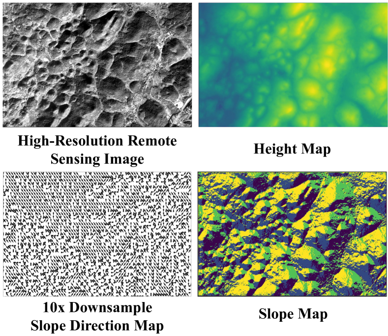
Figure 1: Illustration of High-Resolution Remote Sensing Image, Height Map, 10x Downsample Slope Direction Map and Slop Map based on WHU-TLC dataset (Gao et al. 2021). We use 10x downsampling for the visualization of the slope direction map.

Introduction

Large-scale reconstruction of the earth’s surface provides valuable insights into the earth’s features and is particularly important for applications such as monitoring ecological changes (Spellerberg 2005), detecting geographic information (Jones and Purves 2008), and providing early warnings for natural disasters (Prendes et al. 2014). Remote sensing imagery facilitates cost-effective and extensive earth observation and has become a crucial data source for the task (Whitaker and Juarez-Valdes 2002). Considering that the Earth’s continental regions are primarily composed of terrains, accurate terrain height estimation using remote sensing imagery is crucial for 3D reconstruction of the Earth’s surface and numerous algorithms have been developed for this task with rational polynomial camera (RPC) parameters(De Franchis et al. 2014a; Xiong and Zhang 2010; Meng et al. 2007). However, these classical open-source algorithms for large-scale 3D terrain reconstruction usually use traditional feature extraction operators (Ng and Henikoff 2003) that are not able to fully extract complex terrain surface features, which may lead to error height estimation and subsequently cause reconstruction holes.

Recently, the advancement of deep learning has led to numerous multi-view stereo (MVS) methods that leverage this technology. These methods have shown significant potential in terms of accuracy and efficiency, particularly in close-range and aerial reconstruction using pinhole cameras. However, current methods primarily concentrate on estimating the depth map in accordance with the fronto-parallel planes of a reference view. These methods are not directly applicable to the RPC model (Meng et al. 2007), as it lacks explicit physical parameters to define the front of a camera. To mitigate the differences in imaging geometries between push-broom and pinhole cameras, SatMVS (Gao et al. 2021) introduces a robust differentiable rational polynomial camera warping (RPC warping) module. This module enables deep MVS satellite image 3D reconstruction without the need for epipolar rectification.

In SatMVS (Gao et al. 2021), several methods have been explored to apply differentiable RPC warping to large-scale MVS reconstruction using remote sensing imagery, such as RED-Net (RPC) (Liu and Ji 2020), CasMVSNet (RPC) (Gu et al. 2020), and UCS-Net (RPC) (Cheng et al. 2020). However, these methods primarily adapt the general learning-based MVS framework without considering the specific characteristics of the terrains. These geographical features are pivotal in delineating the earth’s surface, and the oversight leads to low accuracy in height estimation. From the macro perspective, the terrains are typically undulating, while from the micro perspective, the terrains can be defined as composed of countless small planes. In the context of remote sensing height estimation, previous works mainly faced two issues when terrain characteristics were not considered: (1) using equal interval partition might not effectively cover the undulating surface, resulting in inaccurate height estimations; (2) estimating the height for each pixel without taking into account the surrounding pixel height values might cause the estimated height are not in an effective height range for a single plane, i.e., there may be an abnormal height value, which leads to inaccurate height estimation. To address these issues, we propose using slope to measure the Earth’s surface, with subsequent discussions centered around this approach.

The slope is the fundamental characteristic of the earth’s surface to reflect its stability and mobility, and other high-level terrain characteristics are mainly developed based on slope measurement (Varnes 1978; Abramson et al. 2001). Therefore, incorporating slope awareness into a MVS pipeline appears essential for achieving effective large-scale reconstruction of the earth’s surface. Slope, in essence, corresponds to the concept of gradient in mathematics, where it quantifies the rate of change of a variable with respect to another (Liu et al. 1994). In remote sensing imagery, we can analogously view the earth’s surface as comprising numerous small slope surfaces, akin to computing gradients in mathematical functions. By examining how terrain variables change over small distances in various directions, we can infer the slope of the surface. Specifically, in high-resolution remote sensing images, we can assume that a 3×3 pixel plane is the smallest slope surface, and the height values of a single slope surface will not change extremely. Thus the slope for a given pixel can be defined by the difference between the height value of that pixel and the maximum of the height values of the eight neighboring pixels around it, while the slope direction is defined as the direction from the maximum height value to the center pixel. As shown in Figure 1, we can utilize above strategy to obtain the slope direction map based on the height map. This map can then be utilized to refine reconstruction results at both micro and macro levels, offering enhanced accuracy and detail in the reconstructed terrain.

Motivated by the above thoughts, we proposed TS-SatMVSNet, an end-to-end slope-aware framework for large-scale remote sensing terrain reconstruction. Drawing from mathematical gradient concepts, we first compute slopes within small pixel planes and then utilize slope direction maps to enhance reconstruction outcomes in three key aspects. Firstly, in order to constrain the framework, we proposed a slope direction loss between the predicted slope direction map and the pseudo ground truth (GT) slope direction map for implicitly optimizing height estimation results, where the slope direction map is generated by the corresponding height map. Secondly, at the macro level, benefiting from the degree of undulation of the surface that can be measured by the slope, we propose a slope-guided interval partition module by adaptively adjusting the pixel-wise height interval to refine height estimation using slope values. Finally, at the micro level, we design a height correction module by using a 3×3 learnable Gaussian smoothing operator for each small plane to amend inaccurate height values to achieve more accurate height estimation. In summary, by introducing slope and slope direction into the MVS pipeline, our model can effectively fit the complex terrain undulated trend in the remote sensing domain by calculating the slope direction map and being constrained by the slope direction loss. Furthermore, our model has combined two slope-guided modules proposed from the macro and micro levels to further achieve more accurate terrain height estimation. The ablation study has also validated the effectiveness of our proposed modules. Moreover, extensive experiments on several benchmark datasets (e.g.WHU-TLC dataset (Gao et al. 2021), MVS3D dataset (Bosch et al. 2016), US3D dataset (Bosch et al. 2019)) demonstrate that our approach achieves excellent performance and demonstrates competitive generalization ability compared to all-listed methods. Specifically, the results as far as correctness and accuracy exceeded the results of other SatMVS-based methods in a between-method comparison by at least 16% in MAE metric and at least 5% in $<2.5m$ metric at WHU-TLC dataset.

Our main contributions are summarized as follows:

• We propose an end-to-end slope-aware framework TS-SatMVSNet for height for large-scale remote sensing terrain reconstruction.

• We propose a height-based slope calculation strategy to measure terrain undulation and provide a visualization method for the slopes.

• We propose two slope-guided modules from macro- and micro-levels to incorporate the slop information into the MVS pipeline to achieve more accurate height estimation.

• We propose a slope direction loss to constrain the model to improve the accuracy of height estimation in the remote sensing MVS domain.

Related Work

Classical Stereo Algorithms for 3D Earth Surface Reconstruction

3D reconstruction of the Earth’s surface from satellite imagery is primarily accomplished through conventional geometric methods, which can be broadly categorized into two main types. The first type is grounded in the epipolar geometry of satellite images, with the RPC Stereo Processor (RSP) (Qin 2016) serving as a prime example. In this approach, stereo images are initially rectified in accordance with the RPC model. Subsequently, a stereo matching algorithm such as the semi-global matching (SGM) (Hirschmuller 2005) method is employed to estimate disparities. CATENA (Catalyst 2021) employs SGM in conjunction with distributed optimization to automatically generate a high-resolution digital surface model (DSM). Ultimately, these disparity maps are transformed into 3D points within the world coordinate system. The second type involves adapting a complex RPC model into a pin-hole model within a confined area, followed by the application of the stereo/MVS pipeline for reconstruction. Satellite stereo pipeline (S2P) (De Franchis et al. 2014b) rectifies stereo images but approximates the push-broom geometry of small cropped image tiles by a pinhole model, and then performs standard stereo matching. Adapted COLMAP (Schonberger and Frahm 2016) uses plane sweeping to avoid epipolar resampling, to reconstruct the 3D structure from multi-view satellite images. However, these classical methods typically depend on traditional feature extraction operators (Ng and Henikoff 2003) to extract features for stereo matching. These operators may not be fully capable of capturing the features of complex terrain surfaces. This limitation could lead to error height estimation, ultimately causing the reconstruction holes.

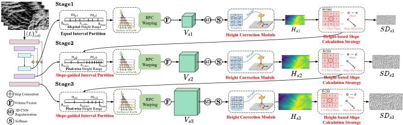
Figure 2: Illustration of overall TS-SatMVSNet. This is a typical multi-stage coarse-to-fine framework. The modules labeled in orange text are the novel modules we propose in this paper. The concepts of ‘all-pixel’ and ‘pixel-wise’ are given by previous related work (Zhang et al. 2023). The details of Height Correction Module and Height-based Slope Calculation Strategy are shown in Fig. 3 and Fig. 5.

Deep Learning Based Multi-View Stereo for 3D Earth Surface Reconstruction

With the development of the artificial intelligence, many deep learning-based Multi-View Stereo (MVS) methods (Yao et al. 2018, 2019; Luo et al. 2019; Yu and Gao 2020) have been proposed to overcome the blemish of traditional methods (Li et al. 2015; Seitz et al. 2006; Stereopsis 2010; Sun et al. 2017) by utilizing the learnable convolution. MVSNet (Yao et al. 2018) firstly proposes an end-to-end MVS framework that extracts features from multiple views by CNNs, thereby achieving high-accuracy reconstruction. P-MVSNet (Luo et al. 2019) proposes a hybrid 3D U-Net to infer a probability volume from the cost volume and estimate the depth maps. R-MVSNet (Yao et al. 2019) uses convolutional GRUs instead of 3D CNNs to regularize the 2D cost maps. Fast-MVSNet (Yu and Gao 2020) proposes a sparse cost volume and a Gauss-Newton layer to obtain the high-resolution depth map. MVSNet++ (Chen et al. 2020) introduces a depth-based attention mechanism designed to produce smoother depth maps. EI-MVSNet (Chang et al. 2024) employs an epipolar-guided volume construction approach for depth map prediction. NR-MVSNet (Li et al. 2023) implements the DHNC aimed at gathering more promising depth hypotheses, which enhances the DRRA modules’ ability to predict more accurate depth maps.

However, current methods primarily depend on the pin-hole camera model to estimate the depth map in accordance with the fronto-parallel planes of a reference view. So it is difficult to directly apply the state-of-the-art deep learning-based MVS methods to satellite imagery with a complex RPC model. Therefore, SatMVS (Gao et al. 2021) attempts to fill this gap by proposing a general deep learning-based MVS framework for satellite images. Specifically, SatMVS proposes a differentiable RPC warping module to apply the SOTA learning-based MVS technology to the satellite MVS task for large-scale Earth surface reconstruction, such as RED-Net (RPC) (Liu and Ji 2020), CasMVSNet (RPC) (Gu et al. 2020), and UCS-Net (RPC) (Cheng et al. 2020). Sat-MVSF (Gao et al. 2023) extends SatMVS (Gao et al. 2021) to provide a comprehensive description of each step involved when modern deep learning-based technology is applied to the task of 3D reconstruction of satellite imagery. RS-MVSNet (Liu et al. 2023) proposes a deep learning-based framework to infer a digital surface model from multi-view optical remote sensing images.

However, these methods primarily adapt the general learning-based MVS framework without considering the specific characteristics of the terrains. This oversight leads to low accuracy in height estimation. In this paper, to overcome this challenge, we attempt to incorporate the characteristics of terrains by proposing an end-to-end slope-aware height estimation network for large-scale remote sensing terrain reconstruction.

Methodology

Pipeline

The overall framework of TS-SatMVSNet is shown in Fig.2. It employs a three-stage coarse-to-fine framework for terrain height estimation. In stage 1, we execute standard MVSNet pipeline to obtain height map, then calculate the slop information based on the height map for later slope-guided interval partition of stage 2/3. And the height correction module adopted across three stages. Specifically, prior to entering the pipeline, a FPN (Lin et al. 2017) is used to extract multi-scale context terrain surface features $\left\{I_{i}\right\}_{i=0}^{N}$ from $N$ input images.

• Stage 1: we use the RPC warping (Gao et al. 2021) based on the all-pixel height range to construct the cost volume $V_{s1}$. And after the regularization and softmax, we adopt a height correction module to amend inaccurate height values for predicted height map $H_{s1}$. Then we follow the height-based slop calculation strategy to obtain the slope map $S_{s1}$ and slope direction map $DS_{s1}$.

• Stage 2: we utilize the slope-guided interval partition based on the slop map $S_{s1}$ and pixel-wise height range to achieve adaptively adjusting the pixel-wise height interval. Similar to Stage 1, after obtaining the cost volume $V_{s2}$, we also adopt the height correction module and height-based slop calculation strategy to process the corresponding item.

• Stage 3: Stage 3 is similar to Stage 2, but with a greater number of height hypothesis planes and a larger scale feature map for improved performance.

After obtaining the height maps and slop direction maps, we adopt the smooth L1 loss (Girshick 2015) and our proposed slope direction loss to constrain the model.

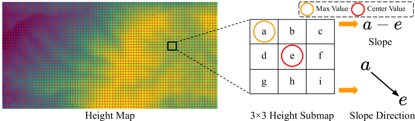
Figure 3: Illustration of Height based Slope Calculation Strategy.

Height based Slope Calculation Strategy

The Earth’s continental regions are predominantly characterized by undulating terrains, with slope serving as a fundamental parameter to depict their undulation, akin to the mathematical concept of gradient (Liu et al. 1994). To incorporate the slope into our MVS pipeline, we assume the terrain as comprised of numerous small planes, each exhibiting slope at a micro level, analogous to the concept of gradient computation. This assumption can transform the Earth’s surface in remote sensing images into a multitude of small slope planes, enabling slope awareness in our MVS pipeline. Based on the assumption, we consider adopting 3×3 pixel planes as the smallest plane in the deep learning-based MVS framework. Then we propose a height-based slope calculation strategy based on above assumption to obtain the slope map and slope direction map without introducing additional supervised information to improve the performance of height estimation.

Specifically, as shown in Fig 3, our strategy can convert the height map to slope map and slope direction map. In order to implement the above strategy, we have defined two calculation criteria for slope and slope direction respectively. Firstly, for the slope calculation, we generate corresponding 3×3 pixel smallest planes for each pixel (achieved by Unfold function of PyTorch (Paszke et al. 2019)). Then, for each smallest plane $p^{3\times 3}(x)$, we take the absolute value of the difference between the maximum height $max(p^{3\times 3}(x))$ and the height value $H(x)$ of the center pixel as the slope value $s=S(x)$ corresponding to that pixel $x$. The formulation of this process as Eq. 1:

$$p^{3\times 3}(x)=\begin{bmatrix}a&b&c\\ d&e&f\\ g&h&i\end{bmatrix}$$ (1)

$$S(x)=|max(p^{3\times 3}(x))-e|$$

Secondly, as shown in Figure 3, the slope direction represents the direction from the center pixel to the maximum height. In order to effectively represent the slope direction, we have established a set of directional codes implemented by PyTorch (Paszke et al. 2019) where adopts the numbers to represents the directions. Specifically, since the size of our smallest plane is 3×3, there are a total of 9 slope directions, which are lower right: 0, down: 1, lower left:2, right:3, vertical:4, left:5, upper right:6, up:7 and upper left:8. Among them, vertical corresponds to the height value of the center pixel being the maximum height, as shown in Fig 4. The exact procedure regarding the slope direction calculation algorithm we describe using pseudo-code:

Figure 4: Illustration of Slope Directional Codes.

input : Height Map

output : Slope Direction Map

initialization;

$p^{3\times 3}$ $\leftarrow$ Unfold(Height Map);

$index_{max}$ $\leftarrow$ Max($p^{3\times 3}$) for each $3\times 3$ plane ;

$S_{diff}$ $\leftarrow$ $p^{3\times 3}$[$index_{max}$] - Height Map ;

if $S_{diff}$ $<$ 0 then

    index1 $\leftarrow$ $S_{diff}$ $<$ 0 ;

   

   $S_{diff}$[index1] $\leftarrow$ -8 ;

   

end if

;

if $S_{diff}$ $>$ 0 then

    index2 $\leftarrow$ $S_{diff}$ $>$ 0 ;

   

   $S_{diff}$[index2] $\leftarrow$ 0 ;

   

end if

;

Slope Direction Map $\leftarrow$ Abs($S_{diff}$ $+$ $p^{3\times 3}$[$index_{max}$]) ;

Algorithm 1 Slope Direction Calculation Algorithm

Through the above two calculation criteria, we can generate the slope map and slope direction map by the height map. The slope map is used in the Slope-guided Interval Partition module. And the slope direction map is used in the Slope Direction Loss, which allows for self-supervised constraint without introducing additional data. In addition, the slope direction map can also be used for visualization, as shown in Fig 1.

Slope-guided Interval Partition Module

In the remote sensing domain, most existing MVS methods (Gao et al. 2021; Liu et al. 2023) employ equal interval partition for pixel-wise height estimation, which may not effectively cover undulating terrain, ultimately resulting in imprecise height estimation. To address this issue, we propose a slope-guided interval partition module, which utilize the slope of each pixel to reallocate the distribution of height hypothesis planes of each pixel. This module desires to allocate more dense height hypothesis planes within the height range with larger slopes, vice versa, relatively sparse planes within the range with smaller slopes. This is done in order to accurately estimate the height of undulating terrain.

Before introducing the height hypothesis plane partition strategy, we firstly introduce the calculation process of the pixel-wise height range. Following the previous MVS methods (Gao et al. 2021; Cheng et al. 2020; Zhang et al. 2023), we also adopt the similar calculated criteria to obtain the pixel-wise height range. Specifically, we utilize previous stage height map $H$ and probability volume $P$ to calculate the pixel-wise standard deviation $\hat{\sigma}(x)$ , which is defined as Eq. 2:

$$\hat{\sigma}(x)=\sqrt{\sum_{m}^{M}P_{m}(x)\cdot\left(d_{j}(x)-H(x)\right)^{2}}$$ (2)

where $M$ is the total number of the height planes, $d_{j}(x)$ represents $j^{th}$ plane of height hypothesis planes of pixel $x$. Then we leverage above results to calculate the pixel-wise height range, the upper and lower boundaries of the pixel-wise height range defined as Eq. 3:

$$H_{min}(x)=H(x)-\hat{\sigma}(x),$$ (3)

$$H_{max}(x)=H(x)+\hat{\sigma}(x)$$

Based on the above upper and lower boundaries of the pixel-wise height range, we propose a slope-guided interval partition to reallocate the height hypothesis planes for each pixel. Specifically, given a height map $H$, we firstly utilize the slope calculation criteria to respectively obtain the slope factors of each pixel, i.e calculate the different $S_{max}(x)$ between the maximum height value and the center pixel $H(x)$ in the 3×3 plane $p^{3\times 3}(x))$, as well as the difference $S_{min}(x)$ between the minimum height value and the center pixel $H(x)$. Then we assign $S_{max}(x)$ as the weight for the range from $H(x)$ to $H_{max}(x)$, and $S_{min}(x)$ as the weight for the range from $H(x)$ to $H_{min}(x)$. Next, we use Eq. 4 to distribute $M$ to the two pixel-wise subranges.

$$M_{l2c}(x)=M\times\frac{S_{min}(x)}{S_{min}(x)+S_{max}(x)}$$ (4)

$$M_{c2u}(x)=M\times\frac{S_{max}(x)}{S_{min}(x)+S_{max}(x)}$$

Thus, we leverage the $M_{l2c}(x)$ and $M_{c2u}(x)$ to respectively calculate the corresponding height interval of the pixel-wise subrange following the Eq. 5:

$$I_{l2c}(x)=\frac{H_{min}(x)-H(x)}{M_{l2c}(x)}$$ (5)

$$I_{c2u}(x)=\frac{H_{max}(x)-H(x)}{M_{c2u}(x)}$$

Finally, we can obtain the reallocated height hypothesis planes to achieve the slope-guided interval partition, as defined by Eq. 6.

$$[H_{min}(x),...,H_{min}(x)+I_{l2c}(x)\times i,...,H(x)]$$ (6)

$$[H(x),...,H(x)+I_{l2c}(x)\times j,...,H_{max}(x)]$$

where $i$ is the enumerated value of $M_{l2c}(x)$, $j$ is the enumerated value of $M_{c2u}(x)$.

Height Correction Module

The Earth’s surface in remote sensing images is composed of countless small slope faces at micro level. Thus the height values of a single slope surface will not change extremely. As we know, Gaussian Filter is a linear smoothing filter, suitable for eliminating Gaussian noise, and is widely used in the noise reduction process of image processing (Ito and Xiong 2000). Since the Gaussian Filter is unlearnable, and its fitting ability is not powerful enough for height estimation of remote sensing images with a large number of data. Furthermore, considering the similarity between the structure of the Gaussian Filter and a convolutional kernel. Inspired by above mechanism, we propose a height correction module by leveraging a 3×3 learnable Gaussian Filter for each small slope surface to amend inaccurate height value. Specifically, as shown in Fig. 5, we firstly construct a general Gaussian Filter with considering the characteristic of height estimation. Then we parameterize the Gaussian Filter as the kernel $K$ of the convolution module to act on the height map to amend the abnormal height noise. The formulation of our height correction module is defined as Eq. 7:

$$K=\left\{\frac{1}{16}i,\frac{1}{8}i,\frac{1}{16}i,\frac{1}{8}i,\frac{1}{4}i,\frac{1}{8}i,\frac{1}{16}i,\frac{1}{8}i,\frac{1}{16}i\right\}$$ (7)

$$\tilde{H}=K\odot H$$

where $\tilde{H}$ is the result of being amended.

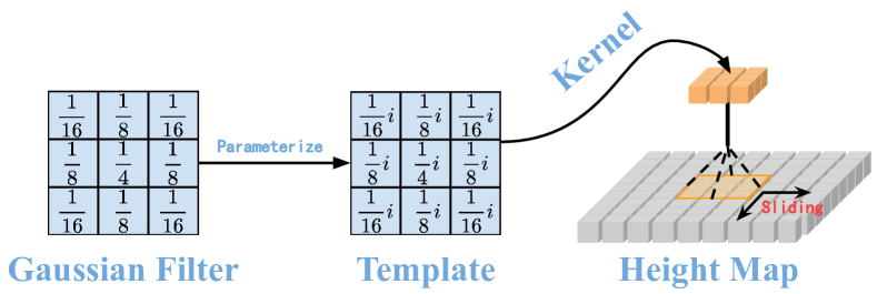
Figure 5: Illustration of Height Correction Module.

Loss Function

To obtain the high-quality outputs of each stage, we adopt two loss functions: Height Map Loss (for height map), Slope Direction Loss (for slope direction map).

Height Map Loss

Height Map Loss is adopted to measure the difference between the GT height map and the predicted height map to constrain the height estimation. Following the previous methods (Gao et al. 2021; Zhang et al. 2023), we adopt same mean absolute difference loss as our loss:

$$L_{h}=\sum_{i=1}^{3}\lambda_{i}\sum_{x\in\mathbf{x}_{\text{valid }}}\|\hat{H}_{s_{i}}(x)-H_{s_{i}}(x)\|_{1},$$ (8)

where $\hat{H}^{s_{i}}$ denotes the GT height map of each stage, $H^{s_{i}}$ denotes the predicted height map of each stage. We set $\lambda_{i}$ to be 0.5, 1.0, 2.0 for each stage, $p_{\text{valid }}$ denotes the valid point set of the GT height map.

Slope Direction Loss

Slope Direction Loss is designed to measure the difference in the slope direction map between the prediction and the pseudo ground truth to constrain our model effectively capture the undulating trend of terrain. However, since current mainstream remote sensing MVS datasets lacks the ground truth (GT) slope direction map, it is difficult to directly calculate the loss term by the slope direction map. Thus, we consider generating a pseudo GT slope direction map $SD$ from the GT height map $\hat{H}$ to participate in the loss calculation. Specifically, we adopt our proposed height based slope calculation strategy to generate the pseudo GT slope direction map. The Slope Direction Loss is defined as the mean squared error (MSE: L2 distance) between the predicted edge map and the pseudo GT slope direction map. By using this loss function, we can ensure that our model is effectively capture the undulating trend of terrain and producing results that are consistent with nearly real-world slope direction maps. The formulation of Slope Direction Loss is defined as follows:

$$L_{s}=\sum_{i=1}^{3}\lambda_{i}\sum_{x\in\mathbf{d}_{\text{valid }}}\|\hat{SD}_{s_{i}}(x)-SD_{s_{i}}(x)\|_{2},$$ (9)

where $\hat{SD}^{s_{i}}$ denotes the GT slope direction map of each stage, $SD^{s_{i}}$ denotes the generated slope direction map of each stage. We set $\lambda_{i}$ to be 0.5, 1.0, 2.0 for each stage, $d_{\text{valid }}$ denotes the valid point set of the GT slope direction map.

Overall Loss

By using the weighted sum of the aforementioned loss terms, we create a comprehensive training criterion for our network. This approach enables us to optimize the network parameters through backpropagation. As a result, our network can learn to produce accurate and robust height maps by minimizing the overall loss, which is a crucial factor in achieving high performance in height estimation tasks.

$$L_{overall}=\lambda_{1}L_{h}+\lambda_{2}L_{s}$$ (10)

where $\lambda_{1}=0.5,\lambda_{2}=0.5$ are hyper-parameters empirically set based on our experiments on the validation set.

Experiment

Satellite MVS Datasets

In the realm of satellite MVS using deep learning, we are presently confronted with a substantial scarcity of training datasets. To our understanding, the only relevant datasets available for this purpose are WHU-TLC (Gao et al. 2021), MVS3D (Bosch et al. 2016), and US3D (Bosch et al. 2019). However, the US3D dataset (Bosch et al. 2019) is aimed at the joint task of semantic segmentation and 3D reconstruction, where the scene variations between the stereo image pairs are not suitable for high accuracy MVS reconstruction, so we opted to use WHU-TLC (Gao et al. 2021) and MVS3D (Bosch et al. 2016) dataset in our pipeline.

WHU-TLC dataset: WHU-TLC (Gao et al. 2021) is a comprehensive satellite multi-view dataset, comprising triple-view images captured by the TLC camera on the Ziyuan-3 (ZY-3) satellite. This dataset includes a multitude of image patches, each accompanied by their respective RPC parameters and corresponding height maps. These height maps are derived from projecting the DSMs onto the images using the RPC parameters. Although theoretically similar to the depth map in a close-range MVS dataset, the height map stores the height information of the corresponding pixel in the image, rather than the depth. Each 5120×5120 image is segmented into 768×384 patches, with a 5% overlap in both horizontal and vertical directions. The dataset contains a total of 5011 training sets.

MVS3D dataset: The MVS3D dataset is a multi-view stereo benchmark for satellite imagery. It comprises 50 WorldView-3 images and airborne LiDAR data, which are used to establish the ground truth. However, the RPC parameters have not been calibrated, leading to a lack of geometric consistency between the matched point clouds and the ground truth. The panchromatic image’s GSD is approximately 0.3 m. The images were acquired over a period spanning from November 2014 to January 2016, while the ground truth data was collected in June 2016. Consequently, significant scene differences exist both among the stereo images and between the images and the ground truth. This implies that reconstructing these scenes poses a formidable challenge, particularly for methods based on deep learning. Furthermore, the MVS3D dataset is considerably smaller than the WHU-TLC dataset and does not provide sufficient training samples for deep learning-based methods.

Evaluation Metrics

In this paper, we adopt the following metrics (similarly adopted in SatMVS(Gao et al. 2021)) to evaluate the quality of DSMs in different datasets:

WHU-TLC Dataset

• MAE: the average of the $L_{1}$ distance over all the grid units between the ground truth and the estimated DSM, the formulation is defined as Eq. 11:

  $$MAE=\frac{\sum_{(i,j)\in D\cap\widetilde{D}}\left|h_{ij}-\tilde{h}_{ij}\right|}{\sum_{(i,j)\in D\cap\tilde{D}}Iver(i,j)}$$ (11)

  where $D$ and $\widetilde{D}$ represent the valid grid cells in the estimated DSM and ground truth, $h_{ij}$ and $\tilde{h}_{ij}$ refer to the height value of the estimation and ground truth in the grid cell in row $i$ and column $j$, and $Iver$ represents the Iverson bracket, which means 1 if $A$ is true and 0 otherwise.

• RMSE: the standard deviation of the residuals between the ground truth DSMs and the estimated DSMs, as defined by Eq. 12:

  $$RMSE=\sqrt{\frac{\sum_{(i,j)\in D\cap\widetilde{D}}\left(h_{ij}-\tilde{h}_{ij}\right)^{2}}{\sum_{(i,j)\in D\cap\tilde{D}}Iver(i,j)}}$$ (12)

• $<$2.5m: the percentage of grid units with an L1 distance error below the thresholds of 2.5 m, the definition of this formula is shown in Eq. 13:

  $$<2.5m=\frac{\sum_{(i,j)\in D\cap\widetilde{D}}Iver(\left|h_{ij}-\tilde{h}_{ij}\right|<2.5)}{\sum_{(i,j)\in D\cap\tilde{D}}Iver(i,j)}$$ (13)

• $<$7.5m: the percentage of grid units with an L1 distance error below the thresholds of 7.5 m, the definition of this formula is shown in Eq. 14:

  $$<7.5m=\frac{\sum_{(i,j)\in D\cap\widetilde{D}}Iver(\left|h_{ij}-\tilde{h}_{ij}\right|<7.5)}{\sum_{(i,j)\in D\cap\tilde{D}}Iver(i,j)}$$ (14)

• Comp: the percentage of grid units with valid height values in the final DSM.

MVS3D Dataset

• RMSE: the standard deviation of the residuals between the ground truth DSMs and the estimated DSMs, as defined by Eq. 12

• $<$1.0m: the percentage of grid units with an L1 distance error below the thresholds of 1.0 m, the definition of this formula is shown in Eq. 15:

  $$<1.0m=\frac{\sum_{(i,j)\in D\cap\widetilde{D}}Iver(\left|h_{ij}-\tilde{h}_{ij}\right|<1.0)}{\sum_{(i,j)\in D\cap\tilde{D}}Iver(i,j)}$$ (15)

• Median: the median value of the absolute error between the estimated DSMs and ground truth DSMs in the valid grid cells, as defined by Eq. 16:

  $$\text{ Median }=\underset{(i,j)\in D\cap\widetilde{D}}{\operatorname{median}}\left(\left|h_{ij}-\widetilde{h}_{ij}\right|\right)$$ (16)

Experimental Settings

In this paper, we primarily adopt two datasets to train and test our model. Specifically, following Sat-MVSF (Gao et al. 2023), we also train our TS-SatMVSNet on the WHU-TLC training dataset (Gao et al. 2021) and evaluate our pretrained model separately on the WHU-TLC test dataset and the MVS3D dataset (Bosch et al. 2016).

WHU-TLC Dataset: During the training phase, TS-SatMVSNet, a PyTorch-based implementation, is trained on the WHU-TLC-V2 dataset using 2x NVIDIA RTX 3090 GPUs, each with 24 GB of memory. The hyperparameters are configured as follows: the batch size is set to 4, RMSProp is chosen as the optimizer, the network undergoes training for 30 epochs, starting with a learning rate of 0.001, this learning rate is halved after the 10th epoch. And a three-stage hierarchical matching approach is employed to deduce height maps from coarse to fine. For the TLC images, the number of input images, denoted as n, is fixed at 3. The numbers of hypothetical height planes and their corresponding intervals are set to [64, 32, 8] and [$\frac{HR_{h}-HR_{l}}{64}$, 5 m, 2.5 m], respectively, where $HR_{h}$ and $HR_{l}$ separately represent the high bound and the low bound of the height range of the current TLC image. In the testing phase, we utilize Sat-MVSF (Gao et al. 2023) designed pipeline to evaluate our pretrained model. We adopt parameters similar to those used during the training phase to infer the height maps. The point clouds generated by these height maps are then incorporated to obtain the Digital Surface Models (DSMs). These DSMs serve as a measure to evaluate the performance of our model by using the evaluation metrics in Sec Evaluation Metrics.

MVS3D Dataset: Due to there are not enough training samples, we use the our model pre-trained on the WHU-TLC Dataset to validate the generalization ability of our TS-SatMVSNet on satellite images. However, since there is currently no very complete and practical material for the MVS3D Dataset (Bosch et al. 2016), under Jian’s (Gao et al. 2023) guidance, we started from scratch to process the MVS3D dataset to obtain the MVS3D dataset that can be used for MVS evaluation. The specific process includes: image cropping, rpc camera model generation, bundle adjustment, view selection. Regarding the specific process, we will open source it along with our code. For specifical experimental setting, we also adopt similar testing configuration to WHU-TLC Dataset, the hyperparameters are configured as follows: the image size is cropped to 3072 × 3072 pixels, the batch size is set to 1, the number of input images, denoted as n, is fixed at 3, the numbers of hypothetical height planes and their corresponding intervals are set to [64, 32, 8] and [$\frac{HR_{h}-HR_{l}}{64}$, 5 m, 2.5 m], respectively.

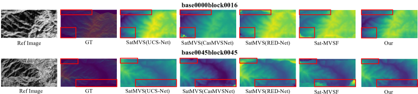
Figure 6: Qualitative results of mainstream deep learning-based methods on two different areas of the WHU-TLC Dataset. The red boxes in the figure are visualized views of the local details respectively.

Methods	Image Size	MAE (m) $\downarrow$	RMSE (m) $\downarrow$	$<$2.5m (%) $\uparrow$	$<$7.5m (%) $\uparrow$	Comp (%) $\uparrow$
CasMVSNet∗	2048 × 1472	2.031	4.351	77.39	96.53	82.33
SatMVS(CasMVSNet)	2048 × 1472	2.020	3.841	76.79	96.73	81.54
UCS-Net∗	2048 × 1472	2.039	4.084	76.40	96.66	82.08
SatMVS(UCS-Net)	2048 × 1472	2.026	3.921	77.01	96.54	82.21
SatMVS-F	2048 × 1472	1.895	3.654	64.82	80.05	-
RED-Net∗	2048 × 1472	2.171	4.514	74.13	95.91	81.82
	5120 × 5120	2.517	4.873	66.42	95.53	81.44
		+15.9%	+7.9%	-10.4%	-0.3%	-0.4%
SatMVS(RED-Net)	2048 × 1472	1.945	4.071	77.93	96.59	82.29
	5120 × 5120	1.946	4.224	77.88	96.54	82.35
		+0.1%	+3.8%	-0.1%	-0.1%	-0.1%
TS-SatMVSNet	2048 × 1472	1.879	3.892	77.92	97.34	82.60
	5120 × 5120	1.882	3.919	77.90	97.32	82.52
		+0.1%	+0.6%	-0.1%	-0.1%	-0.1%

Table 1: The quantitative results on WHU-TLC Dataset (Gao et al. 2021) compared with the deep learning-based MVS methods. ^∗ represents the methods adopt pinhole. ‘-’ represents the default values. ‘blue font’ indicates the percentage of performance improvement from a resolution of 5120×5120 to 2048×1472. Some results are obtained from SatMVS (Gao et al. 2021).

Methods	MAE (m) $\downarrow$	RMSE (m) $\downarrow$	$<$2.5m (%) $\uparrow$	$<$7.5m (%) $\uparrow$
S2P	3.158	10.089	54.96	73.37
SDRDIS	4.496	15.012	47.58	73.57
Adapted COLMAP	2.168	4.714	58.78	76.80
ArcGIS	4.607	10.689	48.88	77.71
CATALYST	3.454	7.939	52.31	82.52
Metashape	2.693	13.047	56.59	75.46
TS-SatMVSNet	1.879	3.892	77.92	97.34

Table 2: The quantitative results on WHU-TLC Dataset (Gao et al. 2021). ^∗ represents the methods adopt pinhole. Some results are obtained from SatMVSF (Gao et al. 2023). Some results are obtained from Sat-MVSF.

Quantitative Results on WHU-TLC Dataset

To demonstrate the effectiveness of our model, we compare our TS-SatMVSNet with two groups of state-of-the-art (SOTA) methods: traditional MVS methods, e.g., adapted COLMAP (Zhang et al. 2019), S2P (De Franchis et al. 2014b), SDRDIS (SDRDIS 2016), ArcGIS (ArcGIS 2022), CATALYST (Catalyst 2021), Metashape (Agisoft 2022), and deep learning-based MVS methods, e.g., RED-Net (RPC) (Liu and Ji 2020), CasMVSNet (RPC) (Gu et al. 2020), UCS-Net (RPC) (Cheng et al. 2020), SatMVSF (Gao et al. 2023).

Comparisons with the traditional MVS methods: For traditional MVS methods, the quantitative results are shown in Table 2, we can observe that our method establishes state-of-the-art performance in all metrics by comparing it to the all of the traditional methods. Specifically, our proposed method has improved by 13.3%, 17.4%, and 32.6% on the MAE, RMSE, and $<2.5m$ metrics respectively compared to the best-performing Adapted COLMAP. And we also improved 13.1% on the $<7.5m$ metric compared to the best-performing CATALYST. We can attribute the superior performance to two special factors:(a) neural operators demonstrate superior adaptability in multi-scale complex scenes, compared to traditional operators such as SIFT (Ng and Henikoff 2003); (b) the incorporation of the terrain slope significantly enhances the scalability and adaptability of our TS-SatMVSNet compared to other traditional pipelines.

Comparisons with the deep-learning-based MVS methods: The quantitative results for the mainstream deep-learning-based MVS methods are shown in Table 1. It demonstrates that our method achieves the highest level in various metrics compared to other SOTA methods. For instance, compared to the SatMVS-F (Gao et al. 2023), our approach can improve the MAE from 1.895 to 1.879 (0.8% performance improvement), the $<2.5m$ from 64.82 to 77.92 (20.2% performance improvement), and the $<7.5m$ from 80.05 to 97.34 (21.6% performance improvement) within the $2048\times 1472$ resolution. Additionally, compared with SatMVS (RED-Net), although our TS-SatMVSNet exhibits relatively lower performance (3.654 vs. 3.892), our method still superior SatMVS (RED-Net) in MAE, $<7.5m$ and Comp respectively, which can improve the MAE from 1.945 to 1.879, $<7.5m$ from 96.59 to 97.34, and Comp from 82.29 to 82.60. We attribute this superior performance improvement to our proposed slope-guided interval partition module, which utilize the slope to reallocate the distribution of pixel-wise height hypothesis planes to obtained more accurate height estimation. Moreover, we also conducted a comparative analysis of the impact of different resolutions on model performance (resolution from $2048\times 1472$ to $5120\times 5120$). From the blue values in the Table 1, we can observe that our proposed TS-SatMVSNet has the least fluctuation across all metrics, e.g., 0.1% $\sim$ 0.6%. On the other hand, RED-Net (Liu and Ji 2020), which also adopts RPC Warping (Gao et al. 2021), exhibits significant result fluctuations across all metrics, 0.3% $\sim$ 15.9%. It is worth mentioning that the incorporation of the terrain slope significantly enhances the scalability and adaptability of our ST-SatMVSNet, which causes our lowest fluctuations across all metrics.

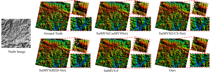
Figure 7: Visualization examples of the DSM results produced by the different methods on the WHU-TLC dataset. The red dash boxes in the figure are visualized views of the local details respectively.

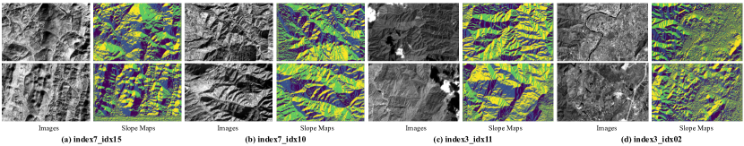
Figure 8: Visualization examples of the slope maps, which calculated from the predicted height maps by our proposed Height based Slope Calculation Strategy (HSCS).

Qualitative Results on WHU-TLC Dataset

To further verify the effectiveness of our proposed method, we have provided several typical qualitative results on the WHU-TLC dataset. Specifically, we have separately compared the height map and DSM results with the state-of-the-art methods. Firstly, as shown in Figure 6, we can observe that our method, as compared to current mainstream deep learning methods, exhibits more accurate results in the height estimation of local details. As demonstrated by the red boxes in the figure, other methods experience artifacts in local areas. This benefits from the incorporation of slope-guided information, our method can effectively capture the undulations of the terrain depicted in the image, thereby precisely estimating height values and consequently reducing the occurrence of artifacts. Secondly, we have further illustrated more DSM results to prove the superiority and effectiveness of our proposed method compared to mainstream methods. The qualitative results are shown in Figure 7, from the comparison of local details in the dashed boxes, it can be seen that our method is capable of reconstructing more complete DSM results compared to the mainstream deep learning methods, e.g. SatMVS, SatMVS-F, which also proves that the more accurate of height estimation of our model can predict. We can attribute this significant improvement is a benefit from our proposed slope-guided interval partition model, which can capture the undulations of the terrain to enhance the ability to perceive terrain changes in order to divide more accurate height intervals and obtain accurate height estimations.

Visualization of Slope Map Results

In the visualization phrase, due to the visual effect of the 10x downsampled slope direction map visualized in the form of a flow map is not intuitive enough (as shown in Figure 1), it fails to effectively prove the reliability of our proposed Height based Slope Calculation Strategy (HSCS). Therefore, we have adopted a new visualization scheme that displays by taking the slope values as inputs. The visualization results are shown in Figure 8, where the slope maps are calculated from the height maps predicted by using our HSCS. Benefit from the superior intuitive visualization results, we can obviously observe that our proposed HSCS can effectively capture the undulations of the terrain, thereby integrating the slope information into the pipeline to enhance the perception of the terrain. It is noteworthy that the comparison between slope maps and the original images very visually demonstrates the effectiveness of our proposed HSCS. Additionally, as shown in Figure 8 (d), some artifacts are present in the obtained slope map, which can be seen from the correspondence with the original image to be generated from the height estimation results of urban areas. Since our initial design was intended for terrain, these urban areas were not considered, suggesting that future integration of further improvement strategies may be considered.

Ablation Study

In this section, we have conducted an ablation study to understand and analyze the contributions of the modules of our architecture. The quantitative results are shown in Table 3 and the qualitative results are shown in Figure 8. Specifically, our ablation studies are mainly divided into two parts: Firstly, we validated the accuracy and advantages of our proposed framework in geographical height estimation. Secondly, we further conducted more ablation analysis to verify the effectiveness of our proposed slope-based modules. Additionally, we set up the SatMVS (UCS-Net) as our baseline.

Effectiveness of the Terrain Height Estimation: As we know, the WHU-TLC Dataset is a multi-view stereo height estimation dataset that contains many different remote sensing scenes, e.g., terrain, urban, and other areas. However, since our scheme is designed for terrain height estimation, scenes from non-terrain areas may not be suitable for our proposed slope-guided manner, thereby affecting the performance of height estimation. This situation is also reflected in the metric of $<$2.5m in Table 1, i.e., our method did not obtain the SOTA on this metric. Thus, we can attribute it to the WHU-TLC test set, which includes some urban scene areas and may affects the performance of our method. Therefore, to further verify the effectiveness of our method in the task of terrain height estimation, we constructed a sub-dataset $\text{WHU-TLC}^{*}$ that only includes earth terrain areas based on the existing WHU-TLC test set and conducted comparative experiments, e.g, index7 folders, index3 folders. The quantitative results are shown in Table 3, we can observe that using purely terrain images to construct the $\text{WHU-TLC}^{*}$ sub-dataset has resulted in a significant improvement in performance across all metrics. Specifically, MAE improved by 4.6%, RMSE by 4.1%, $<$2.5m by 1.4%, and $<$7.5m by 0.5%. We attribute it to our novel slope-guided manner, which can effectively capture the undulations of the terrain and integrate slope information into the pipeline, thereby enhancing the performance of terrain height estimation.

Methods	SIPM	HCM	Dataset	MAE (m) $\downarrow$	RMSE (m) $\downarrow$	$<$2.5m (%) $\uparrow$	$<$7.5m (%) $\uparrow$
Baseline			WHU-TLC	2.026	3.921	77.01	96.54
Baseline + SIPM	$\surd$		WHU-TLC	1.911	3.898	77.83	97.15
Baseline + HCM		$\surd$	WHU-TLC	2.002	3.914	77.25	96.90
TS-SatMVSNet	$\surd$	$\surd$	WHU-TLC	1.879	3.892	77.92	97.34
	$\surd$	$\surd$	$\text{WHU-TLC}^{*}$	1.793	3.732	79.03	97.88
				+4.6%	+4.1%	+1.4%	+0.5%

Table 3: Ablation study on the WHU-TLC Dataset, which demonstrates the effectiveness of different modules of our method. ‘$\text{WHU-TLC}^{*}$’ represents the reconstructed WHU-TLC, which contains pure terrain data. ‘SIPM’ represents our proposed Slope-guided Interval Parition Module and ‘HCM’ represents the Height Correction Module.

Effectiveness of the Slope-guided Interval Partition Module: Moreover, to verify the effectiveness of our proposed slope-guided interval partition module (SIPM), we have validated the ‘baseline + SIPM’ on the WHU-TLC dataset, and the resulting metrics are presented in Table 3. A comparison between Row 1 and Row 2 reveals that the incorporation of slope information to guide the height planes partition, which significantly improves the model’s metrics, including MAE: 2.026 to 1.911, RMSE: 3.921 to 3.898, $<$2.5m: 77.01% to 77.83%, $<$ 7.5m: 96.54 % to 97.15%. The quantitative results effectively demonstrate the validity of our SIPM.

Effectiveness of the Height Correction Module: Furthermore, we have added the Height Correction Module (HCM) with the baseline that involved filtering the slope surface by leveraging 3$\times$3 learnable Gaussian Filter. The experimental results are shown in Table 3 Row 1 and Row 3. We observed that upon integrating our HCM, there was a marked improvement in the performance metrics: MAE decreased from 2.026 to 2.002, RMSE reduced from 3.921 to 3.914, $<$2.5m increased from 77.01% to 77.25%, and $<$7.5m improved from 96.54% to 96.90%. These quantitative results effectively underscore the effectiveness of our HCM.

Generalization on MVS3D Dataset

The MVS3D dataset (Bosch et al. 2016) serves as the benchmark for the IARPA Multi-View Stereo 3D Mapping Challenge and has been extensively utilized as a standard benchmark in prior methodologies (De Franchis et al. 2014b; Catalyst 2021; Gao et al. 2023). To assess the generalizability of our TS-SatMVSNet, we conducted tests using the MVS3D dataset and evaluated the outcomes using the official evaluation scripts. The quantitative results shown in Table 4 demonstrate that our method demonstrates highly competitive performance across all sites and achieved state-of-the-art (SOTA) performance on average evaluation metrics, e.g., 60.635% in $<$1.0m, 0.353m in Median, 2.898m in RMSE. Specifically, we have conducted comparisons with two different types of methods: traditional methods, such as S2P (De Franchis et al. 2014b), Metashape (Agisoft 2022), Adapted COLMAP (Zhang et al. 2019), and deep learning-based methods, e.g, Sat-MVSF (Gao et al. 2023). Compare to traditional methods, our TS-Sat-MVSNet exhibits SOTA performance on the vast majority of sites. For instance, our method can improve the $<$1.0m from 70.4% (S2P) to 71.02% in Site2, Median from 0.531m (SDRDIS) to 0.378m in Site4, and RMSE from 2.102m (S2P) to 1.993m in Site6. Moreover, compared to deep learning-based methods, our method also achieves SOTA or comparable performance on the vast majority of sites. For instance, our method can improve the $<$1.0m from 68.47% (Sat-MVSF) to 73.9% in Site1, Median from 0.338m (Sat-MVSF) to 0.321m in Site3, and RMSE from 2.086m (Sat-MVSF) to 1.993m in Site6. Although our method achieved SOTA performance on most sites and average metrics, there are still some sites where certain metrics are weaker than those of the methods compared above. We posit that the observed variance in model performance across different sites, particularly where our method underperforms in comparison to others, can be attributed to the diverse nature of the MVS3D dataset. This dataset spans a broad spectrum of scenes, encompassing urban landscapes, architectural wonders, and natural environments. Specifically, the complexity and heterogeneity inherent in urban areas may challenge the efficacy of our slope-guided manner, thereby impacting the overall performance of our model in such contexts.

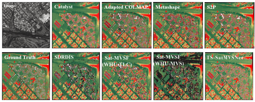
Figure 9: Visualization of the results of DSM evaluation in the first scene of the MVS3D dataset. Some qualitative results are obtained from Sat-MVSF.

Sites	Metrics	CATALYST	Metashape	S2P	SDRDIS	JHU APL	Adapted COLMAP	Sat-MVSF (WHU-TLC)	Sat-MVSF (WHU-MVS)	TS-SatMVSNet
Mean of all sites	$<$1.0m (%)	58.915	56.73	59.49	56.67	55.19	50.38	55.90	51.09	60.635
	Median (m)	0.767	0.495	0.400	0.503	0.883	0.371	0.587	0.368	0.353
	RMSE (m)	4.323	3.464	4.778	4.166	4.896	8.397	3.867	2.957	2.898
Site1	$<$1.0m (%)	72.31	67.61	74.42	69.82	68.09	63.21	68.47	51.44	73.93
	Median (m)	0.353	0.279	0.235	0.304	0.511	0.261	0.34	0.281	0.253
	RMSE (m)	2.913	2.495	2.416	2.772	3.156	3.468	2.83	2.079	2.495
Site2	$<$1.0m (%)	64.57	65.65	70.46	63.82	61.91	55.64	63.78	69.15	71.02
	Median (m)	0.548	0.397	0.348	0.529	0.655	0.264	0.571	0.354	0.341
	RMSE (m)	2.037	1.872	1.836	2.038	2.182	5.464	2.045	1.781	1.731
Site3	$<$1.0m (%)	58.92	54.22	55.06	57.65	54.05	46.7	54.47	50.34	56.33
	Median (m)	0.665	0.506	0.377	0.395	0.827	0.321	0.489	0.338	0.321
	RMSE (m)	4.311	3.898	3.874	3.912	4.581	9.596	3.795	3.124	3.178
Site4	$<$1.0m (%)	43.86	38.68	40.16	41.37	41.94	28.83	39.64	24.4	41.56
	Median (m)	1.466	0.722	0.533	0.531	1.527	0.599	0.698	0.389	0.378
	RMSE (m)	10.319	7.214	12.873	7.844	11.749	19.138	7.8	5.96	5.03
Site5	$<$1.0m (%)	65.58	66.01	70.48	63.65	61.73	64.22	63.59	70.04	71.33
	Median (m)	0.549	0.413	0.377	0.55	0.662	0.35	0.609	0.374	0.377
	RMSE (m)	2.127	1.821	1.772	2.055	2.24	2.777	2.142	1.772	1.990
Site6	$<$1.0m (%)	63.32	62.85	67.47	61.17	57.44	60.88	60.65	66.23	67.03
	Median (m)	0.58	0.446	0.397	0.573	0.744	0.375	0.66	0.395	0.370
	RMSE (m)	2.611	2.105	2.102	2.519	2.63	3.29	2.743	2.086	1.993
Site7	$<$1.0m (%)	42.26	44.66	44.38	40.91	42.16	37.02	41.8	33.41	42.88
	Median (m)	1.355	0.75	0.556	0.767	1.308	0.483	0.846	0.451	0.441
	RMSE (m)	6.192	4.651	6.353	4.652	8.162	13.192	5.869	3.265	3.096
Site8	$<$1.0m (%)	60.50	54.14	53.50	54.95	54.19	46.51	54.82	43.71	61.00
	Median (m)	0.621	0.443	0.375	0.374	0.83	0.316	0.48	0.362	0.339
	RMSE (m)	4.077	3.657	6.996	7.539	4.467	10.254	3.713	3.592	3.667

Table 4: Evaluation results obtained on the MVS3D dataset. The bold figures rank first and the underlined figures rank second in each metric for each site.

Furthermore, we also illustrate the qualitative results of DEM evaluation on the MVS3D testing set. As shown in Figure 9, we can observe that compared to other methods, our reconstructed DSM results do not contain much noise, i.e., there are not many white or black noise points  (both black and white points in the image are considered invalid outliers in the DSM). We attribute this improvement in performance to our model’s accurate height estimation, which enables the synthesis of DSM models with fewer noise points and higher precision. In addition, it is worth mentioning that although our proposed method is not designed for height estimation in urban areas, we can still observe from Figure 9 that the DSM results obtained by our method are comparable. This observation indicates that our method maintains the generalizability for urban areas where these areas are unsuitable for slope-guided manner.

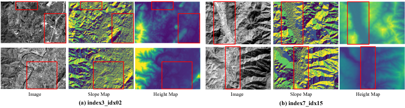
Figure 10: Visualization of some limited cases of mixed terrain and urban scenarios.

Limitation and Consideration

In this study, a slope-aware height estimation pipeline has been leveraged for large-scale earth terrain scenarios, demonstrating significant effectiveness in extensive RS data. While our framework has successfully improved higher accuracy across a variety of benchmarks, it is imperative to acknowledge certain limitations that warrant further investigation:  Inapplicability on Urban Area: Given the significant and abrupt elevation changes encountered within the urban region, the height based slope calculation strategy we have proposed may not be entirely applicable to this specific area. This misalignment could manifest in outcomes artifacts to those illustrated within the red boxes of the slope map presented in Figure 10. Therefore, the integration of slope information into the pipeline could potentially exacerbate the challenges faced by the model in accurately height estimating for this district. Future studies might focus on refining the height estimation for urban regions by designing a specialized module dedicated to accurately capturing the grid structural characteristics inherent to urban architecture.

Conclusion

In conclusion, this paper presents TS-SatMVSNet, a novel slope-aware height estimation framework for large-scale earth terrain reconstruction, which capitalizes on the incorporating slope information to capture the undulations of the terrain to improve the height estimation results. Different from previous methods lacks considering terrain characteristics and leads to low accuracy, TS-SatMVSNet adopts an innovative approach by a height-based slope calculation strategy to calculate a slope map from a height map to further incorporate the terrain characteristics. Specifically, we separately designed a slope-guided interval partition module and a height correction module to achieve more accurate height estimation. Moreover, the overall framework is constrained by two individual losses, e.g., depth loss, slope direction loss. To ascertain the efficacy of TS-SatMVSNet, we meticulously carried out our experiments on two different datasets, e.g., WHU-TLC dataset and MVS3D dataset. Comprehensive experiments conducted on these datasets have underscored TS-SatMVSNet’s considerable impact on terrain height estimation task. Furthermore, through rigorous ablation studies, the crucial role of height-based slope calculation strategy and the incremental benefits of achieving the slope-guided manner have been affirmed, attesting to the robustness and indispensability of each component within our framework. Our future work aims to explore the broader implications of our approach across different domains while striving to refine the precision of height estimation techniques further.

References

- Abramson et al. (2001) Abramson, L.W., Lee, T.S., Sharma, S., Boyce, G.M., 2001. Slope stability and stabilization methods. John Wiley & Sons.
- Agisoft (2022) Agisoft, 2022. Agisoft metashpe. https://www.agisoft.com/.
- ArcGIS (2022) ArcGIS, 2022. Ortho mapping with mosaic datasets—help — arcgis. https://desktop.arcgis.com/en/arcmap/10.5/manage-data/rasterand-images/ortho-mapping-overview.htm.
- Basher (2006) Basher, R., 2006. Global early warning systems for natural hazards: systematic and people-centred. Philosophical transactions of the royal society a: mathematical, physical and engineering sciences 364, 2167–2182.
- Bosch et al. (2019) Bosch, M., Foster, K., Christie, G., Wang, S., Hager, G.D., Brown, M., 2019. Semantic stereo for incidental satellite images, in: 2019 IEEE Winter Conference on Applications of Computer Vision (WACV), IEEE. pp. 1524–1532.
- Bosch et al. (2016) Bosch, M., Kurtz, Z., Hagstrom, S., Brown, M., 2016. A multiple view stereo benchmark for satellite imagery, in: 2016 IEEE Applied Imagery Pattern Recognition Workshop (AIPR), IEEE. pp. 1–9.
- Catalyst (2021) Catalyst, 2021. Catalyst professional – catalyst.earth [www document]. https://catalyst.earth/products/catalyst-pro/.
- Chang et al. (2024) Chang, J., He, J., Zhang, T., Yu, J., Wu, F., 2024. Ei-mvsnet: Epipolar-guided multi-view stereo network with interval-aware label. IEEE Transactions on Image Processing .
- Chen et al. (2020) Chen, P.H., Yang, H.C., Chen, K.W., Chen, Y.S., 2020. Mvsnet++: Learning depth-based attention pyramid features for multi-view stereo. IEEE Transactions on Image Processing 29, 7261–7273.
- Cheng et al. (2020) Cheng, S., Xu, Z., Zhu, S., Li, Z., Li, L.E., Ramamoorthi, R., Su, H., 2020. Deep stereo using adaptive thin volume representation with uncertainty awareness, in: Proceedings of the IEEE/CVF Conference on Computer Vision and Pattern Recognition, pp. 2524–2534.
- De Franchis et al. (2014a) De Franchis, C., Meinhardt-Llopis, E., Michel, J., Morel, J.M., Facciolo, G., 2014a. An automatic and modular stereo pipeline for pushbroom images. ISPRS Annals of the Photogrammetry, Remote Sensing and Spatial Information Sciences 2, 49–56.
- De Franchis et al. (2014b) De Franchis, C., Meinhardt-Llopis, E., Michel, J., Morel, J.M., Facciolo, G., 2014b. An automatic and modular stereo pipeline for pushbroom images. ISPRS Annals of the Photogrammetry, Remote Sensing and Spatial Information Sciences 2, 49–56.
- Gao et al. (2021) Gao, J., Liu, J., Ji, S., 2021. Rational polynomial camera model warping for deep learning based satellite multi-view stereo matching, in: Proceedings of the IEEE/CVF International Conference on Computer Vision, pp. 6148–6157.
- Gao et al. (2023) Gao, J., Liu, J., Ji, S., 2023. A general deep learning based framework for 3d reconstruction from multi-view stereo satellite images. ISPRS Journal of Photogrammetry and Remote Sensing 195, 446–461.
- Girshick (2015) Girshick, R., 2015. Fast r-cnn, in: Proceedings of the IEEE international conference on computer vision, pp. 1440–1448.
- Gu et al. (2020) Gu, X., Fan, Z., Zhu, S., Dai, Z., Tan, F., Tan, P., 2020. Cascade cost volume for high-resolution multi-view stereo and stereo matching, in: Proceedings of the IEEE/CVF conference on computer vision and pattern recognition, pp. 2495–2504.
- Hirschmuller (2005) Hirschmuller, H., 2005. Accurate and efficient stereo processing by semi-global matching and mutual information, in: 2005 IEEE Computer Society Conference on Computer Vision and Pattern Recognition (CVPR’05), IEEE. pp. 807–814.
- Ito and Xiong (2000) Ito, K., Xiong, K., 2000. Gaussian filters for nonlinear filtering problems. IEEE transactions on automatic control 45, 910–927.
- Jones and Purves (2008) Jones, C.B., Purves, R.S., 2008. Geographical information retrieval. International Journal of Geographical Information Science 22, 219–228.
- Li et al. (2023) Li, J., Lu, Z., Wang, Y., Xiao, J., Wang, Y., 2023. Nr-mvsnet: Learning multi-view stereo based on normal consistency and depth refinement. IEEE Transactions on Image Processing .
- Li et al. (2015) Li, Z., Wang, K., Zuo, W., Meng, D., Zhang, L., 2015. Detail-preserving and content-aware variational multi-view stereo reconstruction. IEEE Transactions on Image Processing 25, 864–877.
- Lin et al. (2017) Lin, T.Y., Dollár, P., Girshick, R., He, K., Hariharan, B., Belongie, S., 2017. Feature pyramid networks for object detection, in: Proceedings of the IEEE conference on computer vision and pattern recognition, pp. 2117–2125.
- Liu et al. (1994) Liu, B.Y., Nearing, M.A., Risse, L., 1994. Slope gradient effects on soil loss for steep slopes. Transactions of the ASAE 37, 1835–1840.
- Liu and Ji (2020) Liu, J., Ji, S., 2020. A novel recurrent encoder-decoder structure for large-scale multi-view stereo reconstruction from an open aerial dataset, in: Proceedings of the IEEE/CVF conference on computer vision and pattern recognition, pp. 6050–6059.
- Liu et al. (2023) Liu, N., Wang, P., Xiang, S., Gu, N., Wang, F., 2023. Rs-mvsnet: Inferring the earth’s digital surface model from multi-view optical remote sensing images, in: IECON 2023-49th Annual Conference of the IEEE Industrial Electronics Society, IEEE. pp. 1–7.
- Luo et al. (2019) Luo, K., Guan, T., Ju, L., Huang, H., Luo, Y., 2019. P-mvsnet: Learning patch-wise matching confidence aggregation for multi-view stereo, in: Proceedings of the IEEE/CVF International Conference on Computer Vision, pp. 10452–10461.
- Meng et al. (2007) Meng, H., Liu, Y., Zhang, J., Gong, H., 2007. Positional accuracy in rpc point determination based on high-resolution imagery, in: Geoinformatics 2007: Remotely Sensed Data and Information, SPIE. pp. 1439–1449.
- Ng and Henikoff (2003) Ng, P.C., Henikoff, S., 2003. Sift: Predicting amino acid changes that affect protein function. Nucleic acids research 31, 3812–3814.
- Paszke et al. (2019) Paszke, A., Gross, S., Massa, F., Lerer, A., Bradbury, J., Chanan, G., Killeen, T., Lin, Z., Gimelshein, N., Antiga, L., et al., 2019. Pytorch: An imperative style, high-performance deep learning library. Advances in neural information processing systems 32.
- Prendes et al. (2014) Prendes, J., Chabert, M., Pascal, F., Giros, A., Tourneret, J.Y., 2014. A new multivariate statistical model for change detection in images acquired by homogeneous and heterogeneous sensors. IEEE Transactions on Image Processing 24, 799–812.
- Qin (2016) Qin, R., 2016. Rpc stereo processor (rsp)–a software package for digital surface model and orthophoto generation from satellite stereo imagery. ISPRS Annals of the Photogrammetry, Remote Sensing and Spatial Information Sciences 3, 77–82.
- Schonberger and Frahm (2016) Schonberger, J.L., Frahm, J.M., 2016. Structure-from-motion revisited, in: Proceedings of the IEEE conference on computer vision and pattern recognition, pp. 4104–4113.
- SDRDIS (2016) SDRDIS, 2016. iarpa: My iarpa contest submission. https://github.com/sdrdis/iarpa.
- Seitz et al. (2006) Seitz, S.M., Curless, B., Diebel, J., Scharstein, D., Szeliski, R., 2006. A comparison and evaluation of multi-view stereo reconstruction algorithms, in: 2006 IEEE computer society conference on computer vision and pattern recognition (CVPR’06), IEEE. pp. 519–528.
- Spellerberg (2005) Spellerberg, I.F., 2005. Monitoring ecological change. Cambridge University Press.
- Stereopsis (2010) Stereopsis, R.M., 2010. Accurate, dense, and robust multiview stereopsis. IEEE TRANSACTIONS ON PATTERN ANALYSIS AND MACHINE INTELLIGENCE 32.
- Sun et al. (2017) Sun, L., Chen, K., Song, M., Tao, D., Chen, G., Chen, C., 2017. Robust, efficient depth reconstruction with hierarchical confidence-based matching. IEEE Transactions on Image Processing 26, 3331–3343.
- Varnes (1978) Varnes, D.J., 1978. Slope movement types and processes. Special report 176, 11–33.
- Whitaker and Juarez-Valdes (2002) Whitaker, R.T., Juarez-Valdes, E.L., 2002. On the reconstruction of height functions and terrain maps from dense range data. IEEE transactions on image processing 11, 704–716.
- Xiong and Zhang (2010) Xiong, Z., Zhang, Y., 2010. Bundle adjustment with rational polynomial camera models based on generic method. IEEE Transactions on Geoscience and Remote Sensing 49, 190–202.
- Yao et al. (2018) Yao, Y., Luo, Z., Li, S., Fang, T., Quan, L., 2018. Mvsnet: Depth inference for unstructured multi-view stereo, in: Proceedings of the European conference on computer vision (ECCV), pp. 767–783.
- Yao et al. (2019) Yao, Y., Luo, Z., Li, S., Shen, T., Fang, T., Quan, L., 2019. Recurrent mvsnet for high-resolution multi-view stereo depth inference, in: Proceedings of the IEEE/CVF conference on computer vision and pattern recognition, pp. 5525–5534.
- Yu and Gao (2020) Yu, Z., Gao, S., 2020. Fast-mvsnet: Sparse-to-dense multi-view stereo with learned propagation and gauss-newton refinement, in: Proceedings of the IEEE/CVF Conference on Computer Vision and Pattern Recognition, pp. 1949–1958.
- Zhang et al. (2019) Zhang, K., Snavely, N., Sun, J., 2019. Leveraging vision reconstruction pipelines for satellite imagery, in: Proceedings of the IEEE/CVF International Conference on Computer Vision Workshops, pp. 0–0.
- Zhang et al. (2023) Zhang, S., Xu, W., Wei, Z., Zhang, L., Wang, Y., Liu, J., 2023. Arai-mvsnet: A multi-view stereo depth estimation network with adaptive depth range and depth interval. Pattern Recognition 144, 109885.