An unoriented skein exact triangle in unoriented link Floer homology
Abstract.
We define band maps in unoriented link Floer homology and show that they form an unoriented skein exact triangle. These band maps are similar to the band maps in equivariant Khovanov homology given by the Lee deformation.
As a key tool, we use a Heegaard Floer analogue of Bhat’s recent -surgery exact triangle in instanton Floer homology, which may be of independent interest. Unoriented knot Floer homology corresponds to of the knot in our -surgery exact triangle.
1. Introduction
Heegaard Floer homology, defined by Ozsváth and Szabó [OS04c], is a powerful Floer theoretic invariant of closed, oriented three-manifolds. A closely related invariant for knots is knot Floer homology, defined by Ozsváth and Szabó [OS04a] and independently by Rasmussen [Ras03], which generalizes to oriented links. Link Floer homology categorifies the Alexander polynomial, and satisfies an oriented skein exact triangle [OS04a, Theorem 10.2] that categorifies the oriented skein relation. For unoriented links, there is a closely related invariant, unoriented link Floer homology, defined by Ozsváth, Stipsicz, and Szabó [OSS17b]. In this paper, we show that an algebraic variant of unoriented link Floer homology111See Remark 1.9 for a comparison with the invariant defined in [OSS17b]., , satisfies an unoriented skein exact triangle over the field with two elements.
Definition 1.1.
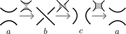
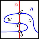
Three links form an unoriented skein triple if the links are identical outside of a ball , in which they differ as in Figure 1.1.
Theorem 1.2.
Let be an unoriented skein triple. Then there exists an -linear exact triangle
A key tool in proving Theorem 1.2 is Claim 5.3, a local version of Theorem 1.3, which may be of independent interest. Theorem 1.3 is a Heegaard Floer analogue of Bhat’s recent -surgery exact triangle [Bha23] for , an instanton Floer theoretic invariant [Flo88] for three-manifolds and links defined by Kronheimer and Mrowka [KM11].
Theorem 1.3.
Let be a knot in . Then given any framing of , there exists an -linear exact triangle
where is the meridian, , resp., is the , resp., -surgery of along , and denotes the Heegaard Floer homology of the three-manifold.
These Heegaard Floer theoretic invariants come in various flavors, for which our exact triangles also hold (see Theorems 4.2 and 4.5). We propose the unreduced hat version, (Definition 1.6) as the counterpart of in Heegaard Floer homology. Indeed, Theorem 1.2 is partly motivated by Kronheimer and Mrowka’s skein exact triangle for [KM11]. Another closely related motivation is to define a spectral sequence from reduced Khovanov homology to knot Floer homology. See Subsection 1.4 for further discussion.

Remark 1.4.
We thank Fan Ye for communicating to the author that a similar analogue of for knots in Heegaard Floer homology222For a knot , put two link basepoints on it and consider the chain complex over where both basepoints have weight . has been suggested in his Miami talk [Ye23].
1.1. Unoriented link Floer homology
Let us define the unoriented link Floer homology groups that we study in this paper.
Definition 1.5.
Let be a -component link in a closed, oriented three-manifold . To define the unoriented link Floer homology of , we need to choose two basepoints for each component of . Let be an admissible, -pointed Heegaard diagram that represents this pointed link . Then the unoriented link Floer homology chain complex is freely generated by intersection points :
and the differential is given by counting both basepoints and with weight :
The unoriented link Floer homology of the link is , the homology of .
The action of the ’s on are homotopic333The same idea as [Zem15, Lemma 5.1] works., and so we also view as an -module, where acts by multiplying by .
We define the unreduced and reduced hat versions of unoriented link Floer homology. We will be lax about issues related to naturality in this section (in particular, basepoints) and postpone the discussion to Section 3.
Definition 1.6.
The (unreduced) hat version of unoriented link Floer homology, , is the homology of the chain complex
Definition 1.7.
A marked link is a link together with a distinguished basepoint (which we call the marked point). The reduced (hat version of) unoriented link Floer homology of a marked link , , is the homology of
where is the link component that the marked point is on.
Given a basepoint on a link , the corresponding basepoint action is multiplication by if the point is on the link component .
For knots, the reduced hat version, , is just knot Floer homology, . We will study some examples shortly, in Subsubsections 1.2.1 and 1.2.2.
We end this subsection with some remarks that explain various aspects of the definitions.
Remark 1.8.
In the definition of the unreduced hat version, we could have quotiented out by any , since multiplication by is homotopic to multiplication by .
Remark 1.9.
All these unoriented link Floer chain complexes can be defined using a more general chain complex defined over . For instance, we have
In [OSS17b], they identify all the ’s together and work with polynomial rings instead of power series rings: the completion of their chain complex is
This is different from ours for links with more than one component, although they are the same for knots.
Remark 1.10.
For simplicity, let us focus on links in . Let be a -component oriented link. Link Floer homology has the Maslov gradings 444There are other conventions that differ from ours by an overall shift . and the Alexander grading [OS08a], which takes values in for some 555If is a knot, then .. The collapsed Alexander grading, obtained by summing the coordinates of , is .
Hence, we can define , the Euler characteristic of with respect to , as an element of the free, rank module over the group ring . This Euler characteristic can be written in terms of the multi-variable Alexander polynomial.
Our unoriented link Floer homology group is singly graded, by the -grading (as in [OSS17b, Subsection 2.1]), since we identify in the sense of Remark 1.9. However, the Alexander grading modulo still exists. Let be the corresponding -torsor.
Hence, we can consider the Euler characteristic666If we want to consider as an unoriented link, then the spaces and should be thought of as - and -torsors living in and , respectively. Also, changing the orientation of a link component changes the -grading by an overall shift, and hence changes the Euler characteristic by a factor of . (Compare [OSS17b, Proposition 7.1].) Viewed this way, these Euler characteristics, up to sign, do not depend on the orientation of . of the unreduced and reduced hat versions (let us mark the th component of ) with respect to the -grading as an element of the free, rank module over the group ring . Then, we have
where is the th unit vector of , ; and is given by (We thank Jacob Rasmussen for this remark.)
Remark 1.11.
We assigned the weights to the basepoints and called multiplication by the basepoint action, to match the convention of equivariant Khovanov homology [Kho00, Lee05, LS22]: the homology groups have a -action, and the basepoint action squared is the -action. Similarly, the unreduced and reduced hat versions are defined analogously to Khovanov homology, which we now recall.
The equivariant Khovanov homology given by the Lee deformation uses the Frobenius algebra over and the multiplication and comultiplication maps are -linear maps given by the following.
Given a link diagram, one considers the cube of resolutions, and uses this Frobenius algebra to build a chain complex. In particular, the vertices of the cube of resolutions chain complex are the equivariant Khovanov homology of unlinks, which is
for the -component unlink. The homology of this chain complex is equivariant Khovanov homology, which corresponds to the minus version777Since we work over a field of characteristic , the homology is not as interesting.. To get unreduced Khovanov homology, or the hat version, we quotient out the chain complex by . If the link has a marked point, then the chain complex can be viewed as a chain complex over , where the action of is given by the marked point in each resolution. The reduced Khovanov homology, or the reduced hat version, is given by quotienting out the chain complex by .
Remark 1.12.
Unlike and , we need two link basepoints on each link component to define unoriented link Floer homology. In link Floer homology, different choices of basepoints give rise to isomorphic homology groups, but the isomorphism is in general noncanonical and interesting [Sar15]. However, moving the two unmarked link basepoints of a link component around the link component induces the identity on unoriented link Floer homology, although it is in general not null-homotopic. We define the hat versions more precisely in Definition 3.4 and show this in Proposition 3.10.
Remark 1.13.
We can define the minus version of unoriented link Floer homology over a polynomial ring instead of a power series ring; this involves assuming strong -admissibility, which depends on the -structure . The unoriented skein exact triangle, Theorem 1.16, holds in this version as well (Remark 4.4), although the -surgery exact triangle, Theorem 1.3, does not (Remark 4.6). We mainly work with power series rings and suppress -structures to simplify the exposition.
1.2. An unoriented skein exact triangle
We will continue to be lax about basepoints in this subsection.
Definition 1.14.
Three (marked) links form an unoriented skein triple if the links and the marked points (if the links are marked) are identical outside of a ball , in which they differ as in Figure 1.1.
Definition 1.15.
A band on a link is an ambient -dimensional -handle, i.e. it is an embedding such that . A link is obtained by a band move on a link if it is given by surgering along a band on .
The following are the three types of bands:
-
•
a band is a non-orientable band if it does not change the number of connected components;
-
•
a band is a split band if it increases the number of connected components;
-
•
a band is a merge band if it decreases the number of connected components.
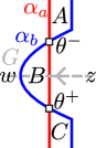
Unoriented skein triples are related by band moves, as in Figure 1.2, and the cyclic order of the three bands is always non-orientable, split, and merge.
Theorem 1.16.
Let be an unoriented skein triple. Then there exist exact triangles in the various versions
where the maps can be interpreted as band maps. The maps are -linear, and also are equivariant with respect to suitable basepoint actions.
If , then the above band maps are homogeneous with respect to the -grading888In general, they preserve relative homological gradings; see Subsubsection 3.3.4..
We show that band maps for planar links coincide with Khovanov homology in Theorem 9.3.
1.2.1. Unlinks and the Hopf link
Recall that link Floer homology cannot have a skein exact triangle without any modifications, as there should be an exact triangle involving the unknot, the Hopf link, and the unknot999In Manolescu’s unoriented skein exact triangle [Man07], the unknots have two extra basepoints each; this doubles the rank of ., but has rank and has rank .
In contrast, the unreduced hat version of unoriented link Floer homology of the unlink with components has rank , and that of the Hopf link has rank . The Hopf link and two unknots indeed form an exact triangle, and in fact all these homology groups are the same as Khovanov homology, as vector spaces.
1.2.2. Trefoil knots
The unoriented knot Floer homology of a trefoil in is
and so the unreduced hat version has rank and the reduced hat version has rank . The rank of the reduced version is the same as the ranks of both reduced Khovanov and reduced instanton Floer homology over any field, but the rank of the unreduced version is the same as the ranks of unreduced Khovanov and unreduced instanton Floer homology over , but not over . This is as expected: similarly, it is conjectured that the and of a three-manifold are isomorphic over ([KM10, Conjecture 7.24], [LY22, Conjecture 1.1]), but they are not isomorphic over ([Bha23, Theorem 1.5], [LY24]).
1.2.3. Comparing with Manolescu’s maps [Man07]
Manolescu’s unoriented skein exact triangle and ours both involve pointed links and maps between them. Let us discuss them for one specific example: a non-orientable band between two unknots in . In this case, the number of basepoints on the knots and the rank of the maps are different: Manolescu’s map has half rank, and our map is zero (as in Khovanov homology).
Recall that if we have an admissible Heegaard diagram with three attaching curves , then we can define a holomorphic triangle counting map
The band maps are for some cycle .
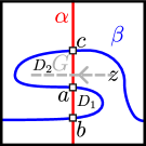
Manolescu’s unoriented skein exact triangle requires the two unknots to each have at least four basepoints. See Figure 1.3101010The crossing of is drawn correctly; see Remarks 2.12 and 2.43 for orientation conventions.: we consider the simplest case where there are exactly four. First, the attaching curves and describe for , i.e. 111111By , we mean the homology of the chain complex freely generated over by intersection points and where the differential counts holomorphic bigons that do not cross any basepoints.. Under this idenfication, the cycle induces the band map . It turns out that all the maps in Manolescu’s exact triangle come from similar looking diagrams.
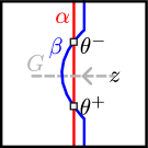
In contrast, our exact triangle requires the two knots to have exactly two basepoints, and they need to be on the same side of the knot with respect to the band, as in Figure 1.4 (we could have chosen instead). See Figure 1.4: similarly, 121212By , we mean the homology of the chain complex freely generated over by intersection points and where the differential counts every holomorphic bigon, where both basepoints have weight , as in Definition 1.5., and under this idenfication, the cycle induces the band map (and also in the unreduced and reduced hat versions). It turns out that all the non-orientable band maps in our exact triangle come from similar looking diagrams; however, the diagrams for the split and merge band maps are different, and these band maps are more complicated to describe.
1.3. A word on the proof
We discuss some key ideas involved in the definition of the split and merge band maps and the proof of Theorem 1.16.
The split and merge band maps involve links with different numbers of link components, and it is not obvious how to define them since we want exactly two basepoints on each link component. (Compare [OS09].) We achieve this by adding a basepoint in the three-manifold when we consider the links with one fewer component (this does not change the quasi-isomorphism type of the chain complex [OS08a, Proposition 6.5]). This basepoint becomes two link basepoints on the link with more components.
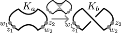
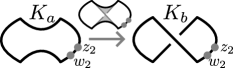
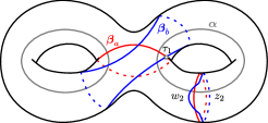
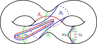
See Figure 1.5: if we consider only or , then we treat the basepoints and as one basepoint (with weight on the three-manifold. When we consider , this basepoint becomes two basepoints (with weight each) on the extra link component.
As usual, we prove the exact triangle by essentially using the triangle detection lemma [OS05, Lemma 4.2] and reducing it to a local computation. We have to work in , i.e. we have to compute the number of certain kinds of holomorphic disks, triangles, and quadrilaterals in , which makes the local computation challenging. Instead of directly carrying out the local computation in , we use a trick that reduces it to two local computations in , which are combinatorial and well understood. This trick utilizes Claim 5.3, a local version of Theorem 1.3, which is a Heegaard Floer analogue of Bhat’s -surgery exact triangle [Bha23]. (See the discussion right before Theorem 4.5 and Section 5.)
Remark 1.17.
Remark 1.18.
The instanton invariants come from the orbifold whose underlying three-manifold is and is the -orbifold points, and the maps in Bhat’s -surgery exact triangle [Bha23] come from orbifold cobordism maps.
We show that splits into -summands where is an -torsor, but we do not discuss further connections with orbifolds in this paper: we do not interpret the maps in Theorem 1.3 as orbifold cobordism maps. However, our maps come from triple Heegaard diagrams, and so it is possible to interpret them as the composition of a link cobordism map (in the sense of [Zem19]) together with a purely algebraic map.
1.4. Motivation
Link Floer homology and instanton Floer homology are closely related to Khovanov homology [Kho00], which is defined combinatorially from an unoriented cube of resolutions. Rasmussen [Ras05] conjectured that the rank of reduced Khovanov homology is always greater than or equal to the rank of knot Floer homology; Dowlin [Dow24] proved this conjecture over .
One challenge in relating Khovanov homology to knot Floer homology lies in the difficulty of finding a suitable generalization of knot Floer homology for links that satisfies an unoriented skein exact triangle131313Dowlin’s spectral sequence uses an oriented cube of resolutions which involves singular knots.. Manolescu’s unoriented skein exact triangle [Man07] in link Floer homology requires additional basepoints on the links. As a result, the page of the corresponding cube of resolutions is not a link invariant, which was shown by Baldwin and Levine [BL12]. Also, Baldwin, Levine, and Sarkar [BLS17] suggested that one should take the Koszul resolution with respect to the basepoint actions on the Khovanov side.
In instanton Floer homology, Kronheimer and Mrowka [KM11] defined a spectral sequence from unreduced Khovanov homology to by defining and iterating an unoriented skein exact triangle for . They also defined a spectral sequence from reduced Khovanov homology to , a reduced version of , which is conjecturally isomorphic to for knots over ([KM10, Conjecture 7.24], [LY22, Conjecture 1.1]). Hence, a Heegaard Floer analogue of and for (marked) links would be a good candidate for a suitable generalization of knot Floer homology from the perspective of Khovanov homology.
Our motivation is to develop a theory in Heegaard Floer homology that is analogous to and , which we hope will include a spectral sequence from Khovanov homology. We propose the unreduced and reduced hat versions of unoriented link Floer homology (Definitions 1.6 and 1.7) as the counterparts of and , and show Theorems 1.3 and 1.16 which are counterparts of theorems in instanton Floer homology.
It is interesting to compare our proposal with the existing conjectures that relate Heegaard Floer homology and . First, for knots, the counterpart of that we propose is indeed . Also, for a three-manifold , is conjecturally isomorphic to over , and a version of our -surgery exact triangle involves , , and (over ), whereas Bhat’s -surgery exact triangle [Bha23] involves , , and .
In Theorem 9.3, we show that for planar links, the band maps in the various versions of unoriented link Floer homology agree with the band maps in (equivariant) Khovanov homology, and hence also with the band maps in and . Hence, if one could iterate our unoriented skein exact triangle, then one would get a spectral sequence from equivariant Khovanov homology to the minus version of unoriented link Floer homology, and also a spectral sequence from reduced Khovanov homology to knot Floer homology.
1.5. Future directions
It is natural to ask whether one can define unoriented link cobordism maps in unoriented link Floer homology, just like . Although we do not discuss this in this paper, it turns out that showing that band maps commute is a key step for iterating our unoriented skein exact triangle and getting spectral sequences from Khovanov homology to unoriented link Floer homology. We hope to achieve this in a later work.
It would also be interesting to be able to compute these band maps (or more ambitiously, the conjectured spectral sequence), either using ideas from bordered Heegaard Floer homology [LOT18] or grid homology [OSS15]. One difficulty in interpreting our maps in grid homology comes from that we only consider links with exactly two basepoints on each component. We do not know whether there are similar band maps in the case where there are more basepoints, such that they form an unoriented skein exact triangle.
Also, we do not deal with signs in this paper and work over a field of characteristic . In contrast, Dowlin [Dow24] has to divide by . It would be interesting to see whether the theorems in this paper hold over .
There are two different -surgery exact triangles in Heegaard Floer homology: there is Theorem 1.3, and also Ozsváth and Szabó’s integer surgery exact triangle [OS04b, Section 9.5], which has two copies of instead of (and the maps are different). In [Nah], we show analogous statements for any positive rational surgery slope: we get (at least) different -surgery exact triangles, one of which generalizes Ozsváth and Szabó’s or -surgery exact triangle. The others involve algebraic modifications of knot Floer homology; more precisely, these are variants (if necessary) of -modified knot Floer homology [OSS17a] for . Note that -modified knot Floer homology is unoriented knot Floer homology.
1.6. Organization
In Section 2, we start by setting notations and recalling some definitions in Heegaard Floer theory in Subsection 2.1. In order to prove Theorems 1.3 and 1.16, we consider local systems that a priori involve negative powers of . We define the type of local systems we consider in Subsection 2.2, and discuss weak admissibility and positivity in Subsection 2.3, which ensure that the differential and (higher) composition maps are well-defined. We use the language of -categories to simplify the homological algebra; we recall this in Subsection 2.4. We set up notations for standard translates in Subsection 2.5 and recall theorems on stabilizations in Subsection 2.6. In Subsection 2.7, we clarify our conventions for link Floer homology, and we define -structures for unoriented links and strong admissibility in Subsection 2.8. We set up conventions for gradings in Subsection 2.9, especially when nontrivial local systems are present. We introduce a simplifying assumption in Subsection 2.10, in which case checking whether gradings exist is simpler.
In Section 3, we precisely define the objects we consider, define the band maps, and show that they are well-defined. Using these notions, we state the main theorem, the unoriented skein exact triangle (and the -surgery exact triangle), in Section 4. In Section 5, we briefly discuss the key steps of the proof, and we carry out the local computations in Sections 6 and 7. Section 7 is also the local computation for the -surgery exact triangle. We use these computations in Section 8 and finish off the proof.
Finally, we compute the band maps for planar links in Section 9.
1.7. Acknowledgements
We thank Peter Ozsváth for his continuous support, explaining a lot of the arguments in this paper, and helpful discussions. We also thank Ian Zemke for his continuous support, teaching the author a lot of previous works, especially [Zem23], and helpful discussions. We thank Deeparaj Bhat for sharing his work on the -surgery exact triangle back in March 2023. We thank John Baldwin, Deeparaj Bhat, Fraser Binns, Evan Huang, Yonghwan Kim, Jae Hee Lee, Adam Levine, Jiakai Li, Robert Lipshitz, Marco Marengon, Sucharit Sarkar, Zoltán Szabó, Alison Tatsuoka, Jacob Rasmussen, Joshua Wang, and Fan Ye for helpful discussions. We also thank Robert Lipshitz, Peter Ozsváth, Jacob Rasmussen, Joshua Wang, and Ian Zemke for helpful comments on earlier drafts of this paper.
2. Preliminaries
2.1. Heegaard Floer homology and local systems
We set up notations and notions that we use throughout this paper. We use local systems that a priori involve negative powers of , as in [Zem23]. Although it is not necesary to consider nontrivial local systems to define the unoriented link Floer homology groups and the band maps, we will use them to prove the exact triangles.
We do not need any new analytic input, and thus we will refrain from discussing the analytic foundations and refer the readers to [OS04c, OS04b, Lip06, LOT16, HHSZ20].
Definition 2.1 ([OS08a, Definition 3.1]).
Given a closed, oriented, genus surface together with a set of basepoints on , an attaching curve is a set of pairwise disjoint, simple closed curves on whose images span a -dimensional subspace of . A multi-Heegaard diagram141414This definition will be slightly modified in Subsection 2.2. is a collection of such a pointed surface together with attaching curves. We assume that attaching curves intersect transversely, and that there are no triple intersections.
Notation 2.2.
We write for one alpha circle. The boldsymbol means a set of alpha circles, and write . If the curves lie in , then, by abuse of notation, also means the image of in and .
Definition 2.3.
Given a multi-Heegaard diagram , an elementary two-chain is a connected component of , and a two-chain is a formal sum of elementary two-chains. A two-chain is nonnegative if its local multiplicities are nonnegative. Denote the -boundary of as (which is a one-chain). A cornerless two-chain is a two-chain for which is a cycle for all . A cornerless two-chain is periodic if it does not contain any basepoints.
Definition 2.4.
A domain is a two-chain together with an ordered sequence of vertices where 151515We can also allow ; we let for simplicity. and for (), such that
for and 161616Not all two-chains lift to a domain.. Let be the set of domains with vertices .
An -domain is a domain with vertices for some intersection points , and a domain with vertices is an -domain for some .
By abuse of notation, we also denote domains as . Also, by abuse of notion, we say a two-chain is in if there exists a domain in whose two-chain is , and we may identify with the corresponding domain.
Remark 2.5.
Note that the two-chain of a domain uniquely determines the domain if the domain has at least three vertices (some of which might be identical). This may not be the case otherwise: for instance, given any -cornerless two-chain for some , for any , there exists a domain in whose underlying two-chain is the given two-chain171717A cornerless two-chain can be lifted to a domain if and only if it has exactly two vertices (which are identical).. (These are not the only examples.)
The Maslov index of a domain can be computed (and/or defined) combinatorially, using the formulas in [Lip06, Section 4] and [Sar11]. Note that , in general, cannot be defined just from the underlying two-chain of 181818Similarly, the monodromy (Definition 2.10) also depends on the vertices of ..
It is shown in [Sar11, Theorems 3.2, 3.3] that is cyclically symmetric in the vertices of , and that is additive, i.e. , with respect to the following composition of domains: given and (), their composition is .
To define the Heegaard Floer chain complex, we need to choose a coefficient ring and assign weights to basepoints. We also equip attaching curves with local systems.
Definition 2.6.
If is a power series ring , denote
Note that this depends on the identification . For an -module , write
A coefficient ring is a power series ring , its quotient, or .
Definition 2.7.
If is the set of all basepoints and is a coefficient ring, then a weight function is a function . Given a weight function , define the weight of a two-chain as
Definition 2.8.
A local system over on an attaching curve is a pair where is a free -module, and is the monodromy: it is a groupoid representation
where is the fundamental groupoid of , and is a groupoid with one object whose automorphism group is . Write , or simply , to signify that is equipped with the local system .
The local systems in this paper will all be specified by an oriented arc on the Heegaard surface that satisfies certain conditions. We define this in Subsection 2.2 and also modify the definition of a Heegaard diagram to a collection or .
Definition 2.9.
A Heegaard datum is a tuple that consists of a multi-Heegaard diagram , a coefficient ring , a weight function , and local systems over for .
Definition 2.10.
Given a Heegaard datum with Heegaard diagram , coefficient ring , weight function , and local systems over , respectively, define the group as a direct sum of ’s:
and define the differential to be an -linear map such that
| (2.1) |
where and is the monodromy of :
We refer to elements of as morphisms from to . In most cases, we omit the subscripts and . Also, we often decorate the symbol : for instance, means that we are working over a power series ring, and means that we are working over some quotient of the power series ring. We will mostly focus on the case.
We get (higher) composition maps 191919The differential is also a composition map. when we have many attaching curves. If are attaching curves with local systems, then the composition map is given by
| (2.2) |
where is the monodromy defined as follows: given a collection of paths in () for intersection points (, ), define the monodromy of as
Given an -domain , its monodromy is .
Remark 2.11.
We need the Heegaard datum to satisfy an admissibility criterion (Subsubsection 2.3.1) for the sum in the definition of to be well-defined. Also, the groupoid representations we consider in this paper will a priori have negative powers of : indeed, they will be maps into . We show in Subsection 2.3.2 that this is not a problem for the Heegaard data that we consider in this paper (see Subsection 2.2).
We need to choose a family of almost complex structure (on , or on , where is a disk with punctures, if we work in the cylindrical reformulation) to define the Heegaard Floer chain complex and the composition maps. In this paper, we will have to work in various different (families of) almost complex structures (for instance, see Section 5). Using the arguments of [Sei08, Section 10c] and [LOT16, Section 3.3], it is possible to show that a generic one-parameter family that interpolates two such (families of) almost complex structures induces an -functor between the -categories given by the two choices, and that this -functor induces isomorphisms on the homology groups. (See Remark 2.25 for a definition of the -categories we consider.)
2.2. Weights and local systems for unoriented link Floer homology
From now on, all the Heegaard data will be of the following form, unless otherwise specified. We recall the conventions for the link we get from such Heegaard diagrams in Subsection 2.7.
The local systems will be specified by an oriented arc on the Heegaard surface. Hence, instead of including local systems as a part of a Heegaard datum, we simply incorporate into the Heegaard diagram: modify the definition of a multi-Heegaard diagram to be a collection of a pointed surface, attaching curves, and possibly also an oriented arc (this will always be drawn dashed and grey). If it includes , then the coefficient ring has a distinguished variable ; or (sometimes we consider a quotient of it or ).
The negative boundary of is a basepoint. For any attaching curve , there is at most one circle that intersects , and the two endpoints of lie in the same connected component of . Furthermore, we assume that there are at most two circles that intersect , and that they are standard, small translates202020These two circles intersect each other at two points, and intersect other circles in the “same way”: see Definition 2.32. of each other, that intersect each other at two points, right above and below . See Figure 2.1 for a schematic near .
If an attaching curve does not intersect , then it has the trivial local system. If some intersects , then we consider the local system where is the rank free -module , and the monodromy sends a path in to , where
The intersection is positive if goes from top to bottom in Figure 2.1.
Furthermore, or for each . If , then there are exactly two basepoints with weight ; we call these basepoints link basepoints. If , then there is exactly one basepoint with weight ; we call these free basepoints212121The basepoint is neither a link basepoint nor a free basepoint.. We also require that for each attaching curve and connected component of , has weight or for some .

Definition 2.13.
We chose a basis for the nontrivial local system . Choose the trivial basis for the trivial local system. These induce -bases on the -Hom spaces. An -generator (or simply a generator) of is of the form , where is an -basis element of and .
Definition 2.14.
If is a two-chain, define the total multiplicity of as
where is the set of link basepoints together with (if exists), and is the set of all free basepoints.
Example 2.15.
Let us consider the first two genus Heegaard diagrams in Figure 2.2, where we work over , and is the distinguished variable.
Let us consider the first diagram. The attaching curve has a nontrivial local system, but ’s local system is trivial. The chain complex is freely generated by as an -module. The differential acts on the generators by
where the first two are given by the two-chain and the last two are given by . Note that if we identify with and with for , then this chain complex is isomorphic to the chain complex given by the third diagram, where we work over , and where we assign the weight to both and .
Let us consider the second diagram. Both attaching curves and have a nontrivial local system. The module is freely generated by () as an -module. The differential is as follows:
In each case, the first summand is the contribution of ; the second summand is that of . Note that the differential is well defined on , but not well defined on as we get a negative power of . Our solution (see Subsubsection 2.3.2) will be to consider the free submodule generated by together with all for except (i.e. replace by ). Then, will be a sub chain complex of .
Remark 2.16.
One can define the composition maps without mentioning local systems, if there is at most one attaching curve with a nontrivial local system. Let us demonstrate this for (we have observed a special case in the first example of Example 2.15). Assume that exactly one of and has a nontrivial local system, and let the coefficient ring be . Then is -linearly isomorphic to the chain complex , where , and we add to the set of basepoints, assign the weight to and , and assign the same weights as before to all the basepoints except and . The -linear chain isomorphism is given by mapping , if is nontrivial; and , is is nontrivial.
2.3. Weak admissibility and positivity
We mainly work in the minus version. Recall that in Subsection 2.2, we have specialized to specific kinds of Heegaard data, which involved local systems that a priori involve negative powers of . Under these assumptions, we first deal with admissibility, which ensures that the sums in Equations 2.1 and 2.2 are well-defined in .
We then deal with positivity, i.e. we show that our maps only involve nonnegative powers of . More precisely, we define a -type sub chain complex of , which we call the space of filtered maps as in [Zem23], on which the other composition maps ( for ) are defined as well. By -type, we mean that is a (free) sub -module of , and that . In our case, positivity is ensured because we have at most two attaching curves with nontrivial local systems222222When we prove the exact triangle, we need to consider two, and fortunately only two.. If at most one of or is a trivial local system, then we will have .
We first record a useful lemma.
Definition 2.17.
Define a grading
for as follows.
First, for , let be the largest integer such that , and define by identifying .
Then, define for the basis elements such that it is multiplicative and , (for instance, ). For where are distinct basis elements and , let
Lemma 2.18.
Let be attaching curves with local systems. Consider generators for and . Assume that there is a domain , and let
If , then
where and .
Proof.
This follows from inspecting Figure 2.3. Note that for this claim, we do not need that only at most two of have nontrivial local systems. ∎
2.3.1. Weak admissibility
There are two kinds of admissibility conditions: strong admissibility and weak admissibility. Strong admissibility lets us work with polynomial coefficient rings by ensuring that for each , there are only finitely many domains with Maslov index , if we restrict to a specific -structure. Weak admissibility lets us work with power series rings by ensuring that there are only finitely many domains that contribute when the coefficient ring is , for each 232323We have not discussed positivity yet, so to be precise, we can only talk about ; in this case, weak admissibility ensures a finite count for each , if the coefficient module is ..
We discuss strong admissibility when there are two attaching curves in Subsubsection 2.8.3; for more than two attaching curves, we only study a restrictive case in Subsubsection 2.10.1. We can work with either weak or strong admissibility for the purpose of this paper if we only consider two attaching curves, but when there are more than two, we will mainly work with weak admissibility, since in some cases, we have to consider the sum of infinitely many polygon maps, as in [OS04b, Section 9].
Definition 2.19.
Let be the set of basepoints together with . The Heegaard diagram is weakly admissible if every cornerless two-chain such that has both positive and negative local multiplicities.
Lemma 2.20.
Proof.
Fix generators for and . For each , we would like to show that there are only finitely many nonnegative domains such that
where 242424Here, identify ..
We can now define and show that it is a chain complex. Similarly, one can check that the higher -relations hold: these are simpler since there are no contributions from boundary degenerations.
Lemma 2.21.
Let us consider a weakly admissible Heegaard datum with attaching curves with local systems . The map on satisfies .
Proof.
The proof follows the usual proof of , which studies the ends of the moduli spaces for domains in with Maslov index . The ends consist of broken flowlines and boundary degenerations, and so equals the contribution from the boundary degenerations. See [OS08a, Theorem 5.5], [Zem17, Lemma 2.1], [HHSZ20, Proposition 7.9]. (Our case is algebraically slightly more complicated as we have nontrivial local systems.)
Let the Heegaard surface be , and let the coefficient ring be where (as in Subsection 2.2, in particular or ), where is the distinguished variable. Let , and let us consider domains . We claim that
where the two-chain of ranges through the connected components of , or the connected components of . This is almost exactly like the case where all the local systems are trivial, but with the added complication that might intersect . However, this is not possible as the two endpoints of lie in the same connected component of (and ).
Let be the number of boundary degenerations with two-chain and vertex . We have
and this is zero since does not depend on (and ). ∎
2.3.2. Positivity
We define the space of filtered maps.
Definition 2.22.
Define the space of filtered maps, , as follows.
-
•
If either or has the trivial local system, then every element of is filtered.
-
•
If both and have nontrivial local systems, then is filtered if for each summand of such that , we have that .
In other words, we only rule out (but allow ) for such that .
The following is the main lemma that ensures positivity. (Compare [Zem23, Lemmas A.3, A.5])
Lemma 2.23.
Let be attaching curves with local systems. Assume that at most two of them have nontrivial local systems. Consider generators for and . If there exists a nonnegative domain , let
If are filtered, then is filtered.
Proof.
There is nothing to show if all the local systems are trivial. Let us assume that and () have nontrivial local systems, and that the rest have trivial local systems. Also, assume that . Let , as in Figure 2.3. We will use the following repeatedly: if and the boundary or intersects , then and . Hence, , , , and . Note that in this case, , and so is filtered.
We divide into a few cases. If , then we we are done if . If , then it must be the case that , for all , and . Hence, or , and . Since , the -boundary intersects .
If , then we are done if . Hence, assume that . Then it must be the case that (and so or ), and for all , and . Hence, we can assume that and do not intersect .
-
•
If , then , and so intersects .
-
•
If and , then .
-
•
If and , then since and do not intersect , . Hence is filtered.
∎
As everything is well-defined, we can now show that is a chain complex, and similarly that the higher -relations hold.
Corollary 2.24.
Let us consider a weakly admissible Heegaard datum with attaching curves with local systems . Then together with is a chain complex.
Proof.
By abuse of notation, we mean whenever we write from now on.
2.4. Twisted complexes
We use the language of twisted complexes in order to nicely package the necessary algebra. We mostly follow [Zem23, Subsection 2.3] and [Sei08, Sections 1b, 3k, 3l, and 3m]. Also compare [LOT16].
2.4.1. -categories and twisted complexes
We work with non-unital -categories over . Our conventions are slightly different from [Sei08], due to the nature of Heegaard Floer homology: we use the homological convention instead of the cohomological convention, and -categories are not necessarily graded. However, the -categories we consider will be graded in some special cases: we say that an -category is graded if the Hom spaces are -graded and the composition maps have degree . When everything is graded, we use the convention that for a homogeneous , the corresponding element in has degree . In other words, shifts the grading down by .
Remark 2.25.
If one wants to justify the use of the language of -categories, the following is one unsatisfying way that works for this paper. Let us say that we have a weakly admissible Heegaard datum where the attaching curves together with the local systems are , such that the local systems are trivial for all but at most two ’s. Also assume that we have made the analytic choices necessary to define the composition maps in Heegaard Floer theory. Then, the -category we work with has objects , and the Hom spaces and composition maps are nontrivial only if the attaching curves are in the correct order, i.e.
When we write , it will be implicit that comes before .
Let be an -category. Then, the additive enlargement is defined as follows. Objects are formal direct sums
where is a finite set, is a family of objects of , and is a family of finite-dimensional vector spaces. Morphisms are defined as a combination of morphisms between the vector spaces and morphisms in :
Similarly, compositions are defined by combining the ordinary composition of maps between vector spaces and morphisms in . The additive enlargment forms an -category.
A twisted complex in consists of an object together with a differential , such that
Seidel assumes that the differential is strictly lower triangular with respect to a filtration on to ensure that the above sum is finite.
Twisted complexes in also form an -category . Morphisms between twisted complexes are the same as before,
but the compositions are different:
Remark 2.26.
If is a graded -category, then its graded additive enlargement is defined exactly the same, except that the finite-dimensional vector spaces are also -graded. It forms a graded -category. Similarly, graded twisted complexes are defined exactly the same, except that we require that the differential has degree . Morphisms between twisted complexes and their compositions are defined exactly the same. The -category of graded twisted complexes, , is graded.
Example 2.27.
-
•
Given an object of , together with the zero differential form a twisted complex in .
-
•
Given objects of and a morphism such that , the mapping cone of is the twisted complex given by and . We write this as
Notation 2.28.
As above, we will usually underline twisted complexes and maps between them. An exception is when the twisted complex comes from a single object , as in the first example of Example 2.27. Also, if and are summands of the twisted complexes and , respectively, and is a map, then we denote the map whose component is and all the other components are as .
2.4.2. -functors and twisted complexes
We will define twisted complexes of attaching curves in one almost complex structure, and deform the almost complex structure. To do this, we have to understand how the -functor induced by deforming the almost complex structure extends to the category of twisted complexes.
Recall that an -functor between two -categories is a collection of a map and multilinear maps for that satisfy the appropriate -relations. If the -categories and are graded, then is graded if has degree for all .
Given an -functor between -categories, the induced -functor is defined as follows: on the objects,
On the morphisms, is defined analogously to , where we combine ordinary composition of maps between vector spaces and .
The induced -functor is defined as follows:
If everything is graded, then is graded as well.
Remark 2.29.
As noted above, we will define twisted complexes of attaching curves and maps between them in one almost complex structure, and will continue talking about them in a different almost complex structure. The latter should be interpreted as the image under , where is the -functor given by deforming the almost complex structure. Note that depends on the choice of the deformation. Fortunately, it will turn out that all the twisted complexes that we consider in this paper are “invariant” under . Furthermore, although the maps between the twisted complexes that we consider might depend on the deformation, it will not matter since we will not care about exactly what these maps are.
2.4.3. Exact triangles and twisted complexes
If are chain complexes, is a chain map, and the mapping cone is quasi-isomorphic to , then we have an exact triangle of their homology groups
In this paper, we care about what the maps in this exact triangle are. Compare with the triangle detection lemma [OS05, Lemma 4.2].
Lemma 2.30.
Let the following be a twisted complex
If the homology of is , then the following sequence of homology groups is exact.
Proof.
One can show this using a diagram chasing argument and the definition of . ∎
Remark 2.31.
That is a twisted complex is equivalent to that is a twisted complex and that the induced map is a cycle. That the homology of is is equivalent to that the induced map is a quasi-isomorphism.
Analogous statements hold if we consider and instead.
2.5. Standard translates
Our main “local computation,” Theorem 4.3, morally says that two specific maps and are homotopy inverses of each other. However, the -categories we work in are not unital: we do not even define . Instead of trying to define units and homotopy inverses, we use standard translates and use some ad-hoc arguments. The definitions in this subsection should be treated as useful shorthands rather than actual definitions.

Definition 2.32.
Let be an attaching curve. A standard translate of is given by slightly translating each circle , such that . If we consider other attaching curves , then we assume that the translate is sufficiently small in the sense that meets and in the same way (see Figure 2.4). Denote the top grading generator of as , or simply . If intersects the oriented arc (i.e. has a nontrivial local system), then the translate is small enough so that also meets and in the same way. We will sometimes denote the generator of as or .
Given a map , define the corresponding maps for and by taking the nearest intersection points. Using these, define standard translates of twisted complexes of attaching curves (see Remark 2.33 for a caveat), and given a map , define the corresponding maps for and as well.
Similarly, if is a twisted complex, then denote the map given by for each summand as , or simply .
Remark 2.33.
We do not claim that the induced map , resp., is always a cycle if , resp., is a cycle, that is always a twisted complex, and that is a cycle. However, they will be for all the cases that we consider in this paper.
Instead of working with homotopy equivalences (and homotopy inverses), we use the following and work with quasi-isomorphisms in the sense of Definition 2.37 252525By Yoneda, they should be the same; but our -categories do not even have ..
Lemma 2.34.
Let us consider a weakly admissible Heegaard datum. Consider a twisted complex of attaching curves with local systems and its small translate , with the same filtration. If is a twisted complex, and if is a cycle that respects the filtration (i.e. lower triangular), and for each summand of , the component of that is from to is homotopic to , then for any other attaching curve , the induced map
is a quasi-isomorphism.
Proof.
The filtrations on induce a filtration on the chain complexes and . With respect to these filtrations, is lower triangular, and the induced maps on the successive quotients are quasi-isomorphisms. ∎
Remark 2.35.
Lemma 2.36 (Derived Nakayama).
Let be a power series ring over a field , and let be two finite, free chain complexes over . Then, a -linear chain map is a quasi-isomorphism if
is a quasi-isomoprhism.
Proof.
Let , and consider the mapping cones of . We show by induction that the homology is trivial if is trivial.
Assume that is trivial. Consider the long exact sequence induced by the short exact sequence
Since is trivial, the map is an isomorphism, and so is trivial by Nakayama’s Lemma. ∎
Definition 2.37.
Two cycles and are morally quasi-inverses if the compositions and satisfy the conditions of Lemma 2.34 modulo , where the coefficient ring is of the form . If such exist, then we say that and are morally quasi-isomorphic.
Similarly, and are morally homotopy inverses if the compositions and are . If such exist, then we say that and are morally homotopy equivalent.
Note that if two maps are morally homotopy inverses, then they are morally quasi-inverses.
Remark 2.38.
Note that we do not claim that being morally quasi-isomorphic or morally homotopy equivalent is an equivalence relation, nor that it does not depend on the choice of the standard translate. In our case, we will have twisted complexes for , and we will show that and are morally quasi-isomorphic. We will deduce that and are morally homotopy equivalent by using Lemma 2.34 and an ad-hoc argument. (There are other ways to finish off.)
2.6. Stabilizations
If the multi-Heegaard diagram is the connected sum of two Heegaard diagrams where the curves are sufficiently simple on one side, we can often reduce the computations to a computation on the other side, by stretching the neck, as in [OS04b, Theorem 9.4]. A subtlety is that we have infinitely many domains that might contribute. One could quotient out the coefficient ring by for large ’s, in which case only finitely many domains contribute; another way is to degenerate the neck and work in a pinched Heegaard surface as in [HHSZ20, Sections 8, 9, and 10] and [HHSZ24, Section 6]. Also compare [Zem23, Subsection 6.1]. In this subsection, we consider the latter and work in a pinched Heegaard surface, but if there are only finitely many domains that could contribute, then all the statements hold for a sufficiently long neck.
Consider a Heegaard datum with Heegaard surface . Let us first discuss genus stabilization, free stabilization, and free link stabilization.

Genus stabilization is where the Heegaard surface is given by connected summing with , and the attaching curves are , which are given by the attaching curve on together with some fixed, essential curve, in a standard way (i.e. the fixed curves are pairwise standard translates of each other) as in Figure 2.5. The coefficient ring and weight functions are unchanged. For a generator , we define
where is the top intersection point in the connected summed .
Free stabilization is similar, but we connected sum with a pointed as in Figure 2.5. The coefficient ring is , where is a new variable, and the weight function is the same except that we assign the weight to the new basepoint. We called this connected summed part the free stabilization region.
Free link stabilization is a slight variant of free stabilization. We connected sum with a doubly pointed , the coefficient ring is , and we assign the weight to both the two new basepoints.
A Heegaard datum is a stabilization of a Heegaard datum if is obtained from by a sequence of genus stabilizations, free stabilizations, and free link stabilizations. To apply [HHSZ24, Proposition 6.5] as stated, we will assume that subsequent genus, free, and free link stabilizations are connected summed at the stabilized region, i.e. a stabilization of a Heegaard datum with Heegaard surface is given by connected summing with a pointed surface at one point262626This is not a serious contraint, as one can always assume this after some handleslides.272727See [Zem21b, Proposition 6.1] for generalized connected sums, where we “connected sum” at more than one point.. We denote the composition of the maps as .
Proposition 2.39 ([HHSZ24, Proposition 6.5]).
If the connected summing region is pinched, then
Another case we need is when we have a triple Heegaard diagram and we connect sum with where is the meridian and and are (standard translates of) the longitude, and get . Note that if we only consider the and attaching curves, then this is a genus stabilization. For a generator or , let where is the unique intersection point in the connected summed . For , let . Then, [HHSZ24, Proposition 6.5] also implies the following proposition.
Proposition 2.40 ([HHSZ24, Proposition 6.5]).
If the connected summing region is pinched, then
We understand the chain complexes of stabilized diagrams. We will need a statement for free (link) stabilizations. Note that for free link stabilizations, since and are in the same elementary two-chain, if and are the chain complexes of free link stabilization and free stabilization, respectively, then we simply have as chain complexes.
Proposition 2.41 ([OS08a, Proposition 6.5], [Zem15, Proposition 6.5, Lemma 14.4]).
Let us consider a weakly admissible Heegaard datum with Heegaard diagram and coefficient ring . Let be a free stabilization of at the point . Then, if the connected summing region is pinched, then the differential for is of the form
with respect to the identification where the two summands consist of the generators that have , resp., .
Furthermore, if is the weight of the connected component of that contains the point , then the map
is homotopic to over .
In particular, if we assume the condition described in Subsection 2.2, then for some , and so the free-stabilization map is a quasi-isomorphism.
2.7. Links and Heegaard diagrams
We assume that the reader is familiar with the definition of link Floer homology [OS08a]. There are various additional data that we can equip to a link; we clarify our conventions.
Definition 2.42.
A minimally pointed link is a link together with a set of (link) basepoints such that for each connected component of , we have .
A suture datum on a minimally pointed link is a choice of one of the two connected components (which corresponds to the component inside the -handlebody) for each connected component .
A -partition of a minimally pointed link is a partition of the link basepoints into -basepoints and -basepoints such that each link component has exactly one -basepoint and one -basepoint.
Let us consider the Heegaard diagram of a Heegaard datum that we considered in Subsection 2.2. In this subsection and Subsubsection 2.8.1, we assume that there is no oriented arc , for simplicity. Equivalently, let be a Heegaard diagram such that for each connected component of , we have or , and there exists a connected component of such that .
This Heegaard diagram specifies a sutured manifold [Juh06, JTZ21] whose boundary components are either a sphere with one suture or a torus with two sutures. Equivalently, this specifies a minimally pointed link inside a pointed three-manifold equipped with a suture datum. (We have ).
Remark 2.43.
We use the convention that the orientation of the Heegaard surface is the same as the boundary of the -handlebody and is different from the boundary of the -handlebody. Also see Remark 2.12. Note that [Man07] uses a different convention (see [BLS17, Section 4.1]); one should mirror the links to translate to our convention.
The sutured manifold corresponding to a suture datum is given as follows. The underlying three-manifold is where means tubular neighborhood. The boundary component has two meridional sutures on , one for each basepoint in ; they are oriented in a way that 282828Our convention is that corresponds to the -handlebody part. is the part that lies over the chosen component of . Also, each connected component of has one suture.
Given a minimally pointed link , there are three different kinds of choices we can make: a -partition, an orientation on , and a suture datum. Two of these determine the third: we use the convention that the link goes from -basepoints to -basepoints in the chosen components of (i.e. the -handlebody). In particular, given a suture datum, a -partition is equivalent to an orientation on . We say that the Heegaard diagram together with such choice represents the oriented link (equipped with the -partition, or a sutured datum).
2.8. -structures for unoriented links
In this subsection, we discuss -structures for unoriented links equipped with a suture datum292929It is in fact possible to define -structures without the choice of a suture datum. in a three-manifold, and discuss relative gradings of the corresponding Heegaard Floer chain complex.
A Heegaard diagram with more than two attaching curves defines a four-manifold with boundary, and in our case, the link basepoints define an embedded surface . It should be possible to define the composition map corresponding to a relative -structure on , such that . We will not discuss this in this paper in full generality. However, we will discuss two crude versions of this idea: one is in the form of a -splitting, which we introduce in Subsubsection 2.9.2; the other case is when the Heegaard diagram is sufficiently simple, which we discuss in Subsection 2.10.
2.8.1. The case
Let be an unoriented, minimally pointed link equipped with a suture datum (Definition 2.42) in a pointed three-manifold . Let us consider a Heegaard datum whose Heegaard diagram represents in . In particular, assume that there is no oriented arc . Let be the sutured manifold given by .
There are two different spaces of relative -structures that we can consider. We can consider , the space of -structures on the sutured manifold , as in [Juh06, Section 4], which comes with a map that specifies the -structure of intersection points. We can also consider , the space of relative -structures on , as in [OS08a, Section 3], which comes with a map . Both spaces are an -torsor.
Given an orientation on , [OS08a, Section 3.6] gives an isomorphism . Hence, we can also define a map 303030In [OS08a], this is denoted as where are the -, -basepoints, respectively, which are determined by and the Heegaard diagram.. If is another orientation on , then [OS08a, Lemma 3.12] for some 313131The homology class is the sum of the meridians of components of on which and are different; we do not need this fact., where is the -linear subspace of spanned by the meridians of components of . Hence, given , we can define its Chern class as the image of under the map , which does not depend on the orientation .
We do not need the entirety of : we consider a quotient. Let us identify .
Definition 2.44.
Define the space of -structures as , which is an -torsor. The above map descends to a map .
For , define its Chern class 323232We can define it as an element in , but this suffices since we only care about the pairing of with elements in . as above. A -structure is torsion if is torsion.
Recall that the coefficient ring is of the form for . Recall that if and only if it corresponds to a link component of ; let be the meridian of in this case. If , let . Let
To talk about -summands, we should view as an -module.
Definition 2.45.
Let be a weakly admissible Heegaard diagram as above. An -generator of is an element of the form where , and . Note that these form an -basis of .
If , define as the -sub chain complex333333Indeed, this is a sub chain complex by [Juh06, Lemma 4.7]. of generated by the -generators such that .
Recall from [OS04c, Section 2.6], [Zem15, Section 4.2] that we can define if is a set of points such that each connected component of and contains exactly one point in . The Chern class of can be computed in terms of the Chern class of : indeed, choose an orientation on and let be the corresponding oriented link, and let be the corresponding -partition. Let be the free basepoints. Then, [OS08a, Lemma 3.13] (also see [Zem19, Lemma 3.3]) implies
| (2.3) |
Lemma 2.46.
Let be a Heegaard diagram as above, and let be a cornerless domain. Then, we have
where is the total multiplicity of (Definition 2.14).
Proof.
Corollary 2.47.
Let be a weakly admissible Heegaard diagram as above, and let . Then, has a relative -grading, where is the divisibility of .
Proof.
Immediate from Lemma 2.46. ∎
Example 2.48.
Consider the weakly admissible Heegaard diagram given by the left side of Figure 2.6. Work over , and assign the weight to both and . The group ; the meridian represents . The -structures and are both torsion, and they differ by . We have
The differential is identically .
Now, consider the right side of Figure 2.6. The group , and . Their Chern class is a generator of ; in particular, it has divisibility . Indeed, there are two domains in with weights , respectively.

2.8.2. The case
Let us consider the case where may exist. In this case, we can formally work with the Heegaard diagram ; define the corresponding and accordingly.
If at most one of and intersects , then Remark 2.16 justifies this. However, if both and intersect , then it turns out that the link is not the link we want: consider the projection map , and assume that is vertical in , i.e. that is the inverse image of the link basepoints on . Then is a split band on ; the link we should consider is the link obtained by surgering along . We will not try to fix this; for our purposes, it is sufficient to consider Chern class summands as follows.
Definition 2.49.
Let us consider a weakly admissible Heegaard diagram as above that may include an oriented arc . Let , be the attaching curves with local systems, and let . Define as the -sub chain complex of generated by the intersection points such that .
2.8.3. Strong -admissibility and
Finally, let us comment on how to define .
Definition 2.50.
The Heegaard diagram is -strongly admissible if all cornerless two-chains such that
have both positive and negative local multiplicities, where is the homology class that represents.
Note that a weakly admissible Heegaard diagram is -strongly admissible for all torsion .
If is -strongly admissible, then we can work over the polynomial ring instead and define . If , similarly define .
Remark 2.51.
Equation 2.3 says that our strong admissibility condition considers the average of the -structures obtained by the different choices of the -basepoints. This has the advantage that the left hand side of Figure 2.6 is strongly admissible with respect to both torsion -structures. In contrast, it is not even weakly admissible with respect to (or ).
2.9. Gradings
Gradings in -categories, if they exist, will turn out to be very useful. For instance, we will use gradings to show that some generators do not arise as summands of certain composition maps.
2.9.1. A homological -grading
Sometimes, the -categories we consider can be given a (homological) -grading, in the sense of Subsection 2.4. Compare [MO08, Section 3], [BL12, Section 5.2]. Note that our notions differ: their periodic domains are cornerless two-chains in this paper.
Definition 2.52.
A Heegaard datum is (homologically) -gradable if whenever and are two domains with the same vertices, then
| (2.4) |
Lemma 2.18 implies the following proposition.
Proposition 2.53.
If a weakly admissible Heegaard datum is homologically -gradable, then the associated -category in the sense of Remark 2.25 can be -graded, such that:
-
•
each -generator is homogeneous;
-
•
has grading , i.e. if is homogeneous, then for or ;
-
•
if and are generators, then .
Similarly, we say that a Heegaard datum if it is homologically -gradable if Equation 2.4 holds modulo . If it is homologically -gradable, then can be -graded.
Note that if the attaching curves are , then we are free to shift the gradings of each by a constant .
Definition 2.54.
We use the convention that if is a small, standard translate of , then has grading 343434If the local systems are trivial, then can be viewed as an element of . Our convention is different from the absolute -grading of , which is ..
2.9.2. An Alexander -splitting
The Heegaard data that we consider will often not be -gradable. However, the corresponding -category can be given a nice -splitting in the sense of Propositon 2.57. For links in , this is the relative, collapsed Alexander -grading, and in general, it is closely related to the -splitting discussed in Subsection 2.8. Note that now, we have to deal with the case where is present.
Definition 2.55.
A Heegaard datum is (Alexander) -splittable if whenever and are two domains with the same vertices, we have modulo .
To talk about the corresponding splitting in the -category, we consider not as an -module, but as an -module, as in Subsection 2.8. If exists, then one of the ’s is the distinguished variable .
Definition 2.56.
An -generator of is of the form where is an -basis element of , , and . We write for . Note that these form an -basis of .
Let for and be -generators. Let be the set of domains such that for some nonzero .
A similar idea as above gives the following proposition.
Proposition 2.57.
If a weakly admissible Heegaard datum is -splittable, then the associated -category has a -splitting in the following sense:
-
•
The chain complexes are -graded, and satisfies the three conditions in Proposition 2.53. In particular, the summands and are -modules. We denote this grading as for a homogeneous element , and call it the Alexander -grading.
-
•
Let for and be -generators. If there exists a domain , then
In particular, the composition maps have degree .
As before, we use the convention that has grading .
Example 2.58.
Remark 2.59.
Note that this -splitting does not see the Maslov index of domains: it only sees whether domains exist. The second condition of Proposition 2.53 implies that whenever we have a -splitting, then the -functor induced by changing the almost complex structure preserves the splitting, i.e. has degree for all .
Remark 2.60.
We can consider twisted complexes in this setting as well, in which case we add the condition that the differential is homogeneous of degree . The composition maps and the functor induced by changing the almost complex structure are homogeneous of degree .
2.10. Homologous attaching curves
Definition 2.61.
Two attaching curves Heegaard surface are homologous if they span the same subspace of .
Note that whether two curves are homologous do not depend on any basepoints on .
In this subsection, let us consider a Heegaard diagram (and possibly also ) such that the ’s are pairwise homologous and also the ’s are pairwise homologous353535If all the attaching curves are homologous, then we also are implicitly making a choice of ; i.e. we choose which ones are the ’s and which are the ’s..
Under this assumption, it is easier to check whether the Heegaard datum is -gradable or -splittable. Similar statements to the results in this subsection hold when the attaching curves are cyclically permuted.
Lemma 2.62.
If are domains with the same vertices, then there exist cornerless domains for where or 363636In fact, this lemma holds for for any ., such that
Proof.
Let us consider the case where ; the other case follows similarly. Let be the difference of the underlying two-chains. Recursively define for such that the -boundary of the two-chain is empty for . Similarly define for such that (all the -boundaries and) the -boundary of the two-chain is empty for . Let be the -cornerless domain with underlying two-chain . ∎
Corollary 2.63.
If all cornerless domains373737In particular, they have two vertices. satisfy , then the Heegaard datum is -gradable. If they satisfy modulo instead, then the Heegaard datum is -splittable.
Proof.
This follows from Lemma 2.62 and the additivity of and . ∎
Lemma 2.62 is equivalent to that a cohomology class on the corresponding four-manifold [OS04c, Subsection 8.1] is determined by its restriction to the boundary (minus one boundary component).
Lemma 2.64.
Let be a domain. If the -structures are torsion for , then .
Proof.
Let be the set of free basepoints. If exists, for the purpose of this Lemma, consider as link basepoints and replace with , and let us choose which link basepoints are -basepoints; write .
We can define the - structure of and its Chern class . The key property we use is that restricts to where . Let be the corresponding oriented link; then we have by Equation 2.3.
Recall the identification
where be the -handlebody. For each pair of link basepoints, choose an oriented arc on from the -basepoint to the -basepoint, and let be obtained by adding the above oriented arc to an oriented arc on from the -basepoint to the -basepoint. Then the oriented link is represented by the class under the above identification. Using the above identification together with that the restriction map is induced by the projection map , one can write in terms of and the ’s. Combining everything, we get . ∎
The above proof also shows that if the torsion hypothesis is removed, then there is a relation between the ’s.
Proposition 2.65.
Let us consider a weakly admissible Heegaard datum whose underlying Heegaard diagram is as in the beginning of this subsection. Let be the three-manifold obtained by attaching curves and 383838The three-manifold does not depend on ., and choose . Consider the -category whose objects are the attaching curves (equipped with local systems), and
for all and ; if , then define .
Then, is homologically -gradable.
Proof.
2.10.1. Strong -admissibility
We can define strong -admissibility in the context of this subsection. Compare [OS04c, Definition 8.8 and Section 8.4.2] and [Zem15, Section 4.8].
Given a cornerless two-chain , by identifying the ’s together and the ’s together, we can define the homology class of as an element in .
Definition 2.66.
Let the Heegaard diagram and the three-manifold be as in Proposition 2.65. The Heegaard diagram is -strongly admissible for if all cornerless two-chains such that
have both positive and negative local multiplicities.
If are two domains with the same vertices; if there exist some for which have an -vertex , assume 393939The Chern class does not depend on by Lemma 2.64.. Consider the cornerless two-chain : Lemmas 2.62 and 2.46, together with the additivity of and , imply that
Hence, Proposition 2.65 works for as well, if we further assume that the Heegaard diagram is -strongly admissible.
3. Band maps in unoriented link Floer homology
The goal of this section is to precisely define the objects we consider, to define the band maps, and to show that they are well-defined. Compare [Zem19, Section 6] and [Fan17]. Note that the objects we consider are different, and hence the band maps are different as well. The band maps we consider are different from [Fan17] even for non-orientable bands: Fan chooses “the other generator,” i.e. the generator that corresponds to in the left hand side of Figure 3.3.
We assume that the reader is familiar with the definition of link Floer homology [OS08a].
3.1. Bands and balled links
In this subsection, we introduce the notion of a balled link and define its unoriented link Floer homology. We first explain the motivation behind considering balled links. Recall from Definition 1.5 that we needed exactly two link basepoints in each link component to define unoriented link Floer homology. Hence, the merge and split band maps involve links with different number of basepoints. As in the discussion of Subsection 1.3, to go around this issue, we free-stabilize our ambient manifold when we consider the link with fewer basepoints.
Figure 3.1 is a diagram of a kind of split band that we consider. The link has two link basepoints and , but there is also a free basepoint in the underlying three-manifold. Band surgery along the specified band creates a new link component (the left hand side part of ). We added the free basepoint so that after we do this band surgery, we can make the basepoint into two link basepoints of the left hand side component (compare the Heegaard diagram). However, to do this, we have to isotope the left hand side component so that it goes through (and ). Hence, the link , the basepoints , and the band do not uniquely determine , let alone the isotopy.
We introduce baseballs and consider balled links to specify and the isotopy up to choices that do not affect the unoriented link Floer homology and maps between them: we specify a baseball that intersects in an interval, and isotope the link inside the baseball . (We will also let .)
Considering baseballs and balled links also has the advantage that the following can be encoded in a nice way: in this paper, we only consider -bands in the sense of [Zem19, Section 6.1], which in effect means that the two link basepoints in each link component are “very close to each other” with respect to the bands, and that we treat the two basepoints as one basepoint. This is encoded as that each link has one link baseball (one should think of baseballs as being very small and very round), which contains these two basepoints. In other words, the link baseballs mark the -handlebody part of the link.

Definition 3.1.
A balled link in a three-manifold is an (possibly empty) unoriented link together with a finite, ordered sequence of baseballs , such that they are pairwise disjoint and for each baseball , it is either disjoint from , or there exists a small neighborhood such that is diffeomorphic to . It is possible that the underlying link is empty, but we require the balled link to have at least one baseball.
Each baseball is labelled as a link baseball or a free baseball, and each baseball is either marked or unmarked. For each link component, there is exactly one link baseball that it intersects, and every link baseball has to intersect . It is possible that none of the baseballs are marked.
To define the unoriented link Floer chain complex of a balled link , we define what it means for a Heegaard datum to represent the balled link . To define this, it is convenient to first define an auxiliary datum for .
Definition 3.2.
Let be a balled link with baseballs . An auxiliary datum for is a tuple of an oriented link , link basepoints , and free basepoints that satisfies the following.
-
•
The sets consist of (link) basepoints , respectively, for each link baseball .
-
•
The set consists of basepoints in the interior of for each free baseball .
-
•
The link (ignoring its orientation for now) is obtained from by isotoping in the interior of each free baseball so that does not intersect the free basepoints .
-
•
The components of that are contained in the link baseballs go from a -basepoint to a -basepoint. (Recall Subsection 2.7.)
Definition 3.3.
Let be a balled link, and let be an auxiliary datum for it. A Heegaard datum represents the auxiliary datum if it satisfies the following.
-
•
The Heegaard diagram represents the pointed link inside the pointed manifold .
-
•
The coefficient ring is , where the ’s and the weight function are as follows: (recall that the baseballs are ordered) if the th baseball is a link baseball, then and we assign the weight to both link basepoints corresponding to . If the th baseball is a free baseball, then and we assign the weight to the free basepoint corresponding to .
A Heegaard datum represents if there exists an auxiliary datum for that the Heegaard datum represents.
We define the unoriented link Floer chain complex of a balled link, and hence the unoriented link Floer homology of a balled link. We will show in Proposition 3.7 that the chain complex is well defined up to chain homotopy equivalence, and also show naturality, i.e. that we can choose the homotopy equivalence up to homotopy.
Definition 3.4.
Let be a balled link, and let us choose a weakly admissible Heegaard datum that represents . The unoriented link Floer chain complex of is . Define the infinity version as
If the marked link baseballs are and the marked free baseballs are for , then define the hat version as
If none of the baseballs of are marked, then we do not define the hat version; instead, we consider a new balled link given by together with a marked free baseball (or equivalently, together with a unlinked, marked unknot), and consider instead. Note that is isomorphic to the homology of .
Remark 3.5.
We require at least one of the baseballs to be marked to talk about the hat version, although we could have defined it as . This is to explicitly keep track of the marked point that corresponds to the variable we quotient out by. Our definitions follow the definitions of and (also compare with unreduced/reduced Khovanov homology), although our definitions are slightly more general as we allow more than one link component to be marked. In this generalized version, of a link is the hat version of the unoriented link Floer homology of a corresponding balled link where every component is marked.
Recall that there has to be exactly one “marked point” on the link to define , and that of an unmarked link is defined as the of the marked link , given by adding a unlinked, marked unknot to . For and , there are no “basepoints” on unmarked link components, and so Dehn twisting along an unmarked link component induces the identity. Although we use basepoints in unoriented link Floer homology, the last statement is true in unoriented link Floer homology as well, by Proposition 3.10.
As usual, the infinity version is simple.
Proposition 3.6.
Let be a balled link in , and let the coefficient ring be . Then does not depend on the underlying link. In other words,
Proof.
This argument is standard. Consider a weakly admissible Heegaard diagram for . We can also assume that is also weakly admissible. Let be the usual, unoriented link Floer chain complex, and let the corresponding weight function be . Let be the chain complex whose underlying group is the same as that of , but if the th baseball is a link baseball, then assign the weight to the -basepoint corresponding to and assign the weight to the -basepoint corresponding to . If the th baseball is a free baseball, then let and assign the weight to the free basepoint corresponding to . Let this new weight function be .
We claim that and are isomorphic as chain complexes over . Fix an intersection point , and for each , choose a domain . Then the -linear map given by
is a chain map, since for any cornerless two-chain (indeed, for all ). It is an isomorphism since it has an obvious inverse. ∎
The homology groups , , and are well-defined as groups. See [JTZ21], [HM17, Proposition 2.3], [Zem19, Proposition 3.5].
Proposition 3.7 (Naturality).
Let be a balled link in a three-manifold . Given two Heegaard data that represent , there is a chain homotopy equivalence
over the coefficient ring , which is well-defined and functorial up to homotopy.
Proof.
The statement holds if the auxiliary datum is fixed, by [JTZ21]. We would like to define a chain homotopy equivalence, canonical up to homotopy, for two choices of auxiliary data.
For two choices of link basepoints , the chain homotopy equivalence is given by the basepoint moving map. We move the link basepoints only inside the corresponding link baseball, and so this is well-defined up to homotopy.
For free baseballs, given two choices of the free basepoint and the push-off of the link away from the free basepoint, we claim that the chain homotopy equivalence that is induced by isotoping the link and the basepoint inside the free baseball does not depend on the isotopy, up to chain homotopy. First note that the basepoint moving map corresponding to a meridional loop is homotopic to the identity, since it can be realized as a free-stabilization region going around the corresponding link basepoint. (We thank Ian Zemke for pointing this out: that using [MO10, Proposition 6.2] and/or [Zem15, Proposition 14.20] is unnecessary.) Now, a map given by isotoping the link and the basepoint is homotopic to the composition of the homotopy equivalences (canonical up to homotopy) induced by first pushing the basepoint to the boundary of the free baseball, then isotoping the unknotted strand (intersection of the link and the free baseball) inside the interior of the free baseball, and then moving the basepoint back to where it was. Indeed, this is easy to check if the isotopy is “small,” i.e. when we can move the basepoint to the boundary and back without intersecting the support of the isotopy, but any isotopy is a composition of small isotopies.
Finally, consider both reversing the orientation of a link component of and swapping the labels of the two corresponding link basepoints at the same time. (Note that only doing one of these does not result in an auxiliary datum for the same balled link.) Given a Heegaard diagram for one of these, swapping the labels of the two relevant link basepoints results in a Heegaard diagram for the other. This induces an isomorphism between the chain complexes, and we can check that this is well-defined, squares to the identity, and commutes with all the above maps. ∎
Remark 3.8.
In fact, since the coefficient ring is of the form where are the variables corresponding to the unmarked free basepoints, we have that any two choices of the unmarked free basepoints give canonically isomorphic homology groups, since in [Zem15, Proposition 14.20], only the part survives in homology. (Compare [Zem15, Corollary 14.19].)
Remark 3.9.
The space of -structures for all the different choices of auxiliary datum are canonically identified; and so we can consider and define for . These are also canonical in the above sense.
If we only want to consider finitely many holomorphic disks, then we can work with -strongly admissible Heegaard diagrams (Definition 2.50). Hence, we can also work over polynomial rings and define .
Proposition 3.10.
Let be a balled link. Then, Dehn twisting along an unmarked link component induces the identity on both and .
Proof.
We use the explicit formula given in [Sar15], [Zem17, Theorem B]. Although we have free baseballs, we can consider our chain complex as a canonical direct summand of the chain complex given by putting an unknotted unknot for each free baseball so that they intersect, and change its label to a link baseball (compare the discussion at the start of Subsection 3.3). Hence, the formula still holds.
Let be the two basepoints on the link component that we Dehn twist along. For notational convenience, let be the variable that they correspond to, and let be the other variables. The point is that the coefficient ring is for some . Recall that we define
and that is defined similarly. The map induced by the Dehn twist is
This is the identity on homology, since is on homology by the discussion right before [Zem15, Corollary 14.19] and is also on homology [Zem17, Lemma 9.7]. Indeed, is given by differentiating the coefficients of considered as a matrix with entries in , with respect to , as in [Zem15, Remark 14.12]. The argument of [Zem17, Lemma 9.7] shows that
is an -linear chain homotopy . ∎
Definition 3.11.
A band on a balled link is a band on the underlying link that does not intersect any of the baseballs. A balled link is obtained by a band move on a balled link if the underlying link is obtained by a band move on the underlying link , the orderings of the baseballs are the same, and the labels and the markings of the balls of and are the same, except that
-
•
if the band is a merge band, then exactly one unmarked link baseball of becomes an unmarked free baseball;
-
•
if the band is a split band, then exactly one unmarked free baseball of becomes an unmarked link baseball.
Note that if the band is a merge or a split band, then the label of at least one baseball has to change in order for to be a balled link. Also note that the baseball that changes label in the above definition is never marked.
3.2. Heegaard triple subordinate to a band
To define band maps, we first define what it means for a Heegaard triple to be subordinate to a band. Since the baseballs’ labels might change depending on the type of the band, we handle each band type separately.
We closely follow [Zem19, Section 6.1]; note that our bands are always -bands. Also see Figure 1.5. Also compare [OS06, Section 4.1].


3.2.1. Non-orientable bands
Definition 3.12.
Let be a non-orientable band from a balled link to . A tuple of auxiliary data and for and , respectively, is adapted to if:
-
(1)
the basepoints for and are the same, i.e. , , and ; and
-
(2)
is given by surgering along .
Define the sutured manifold obtained from as follows. On , we add meridional sutures for each basepoint of , such that 404040Our convention is that corresponds to the -handlebody part. corresponds to the parts of that live over the connected components of that are contained in the link baseballs. Also, add one suture to each connected component of .
Let be the connected component of that intersects the band , let be the points that live over , and let . In particular, is a solid torus, and is a torus minus two disks. See Figure 3.2 for a schematic.
Definition 3.13.
Let be balled links, and let be a non-orientable band from to . Let and be auxiliary data for and that are adapted to . We say that the Heegaard triple
is subordinate to and the auxiliary data and , if:
-
(1)
The diagram corresponds to the sutured manifold defined above.
-
(2)
The circles are standard translates of .
-
(3)
Let be as above. Let be the closed curve that is defined up to isotopy (one can show this, for instance, by an innermost disk/arc argument) by the property that bounds a disk in , such that does not intersect and is non-separating in . Similarly, let be the closed curve that bounds a non-separating disk in , that does not intersect .
Then, is a closed curve that is obtained by projecting onto and is a curve that is obtained by projecting onto .
A Heegaard triple is subordinate to , if there is some choice of auxiliary data for and adapted to , such that the Heegaard triple is subordinate to and those auxiliary data.
3.2.2. Merge and split bands
Let us first consider merge bands.
Definition 3.14.
Let be a merge band from a balled link to . Let be the link baseball of that becomes a free baseball in . A tuple of auxiliary data and for and , respectively, is adapted to if:
-
(1)
if and are the two basepoints that correspond to the link baseball , then , , and ; and
-
(2)
in the complement of the baseball , coincides with the link given by surgering along .
Define the sutured manifold obtained from using the exact same definition as in Subsubsection 3.2.1. Define in the same way as well. In this case, is a -ball, and is a sphere minus four disks. The tangle is a -ended trivial (i.e. rational) tangle. Let be the tangle given by surgering along . Note that . See Figure 3.2 for a schematic.
Definition 3.15.
Let be balled links, and let be a merge band from to . Let and be auxiliary data for and , respectively, adapted to . We say that the Heegaard triple
is subordinate to and the auxiliary data and , if:
-
(1)
The diagram corresponds to the sutured manifold defined above.
-
(2)
There exists a path in between and that intersects the circle at exactly one point, and is disjoint from all the other -circles and all the -circles.
-
(3)
The circle bounds a disk in such that , where are as in Definition 3.14.
-
(4)
The circles are standard translates of .
-
(5)
Let be as above. Let be the closed curve (defined up to isotopy) that bounds a disk in , such that does not intersect and separates into two components, such that each component has one component of . Similarly, let be the closed curve that bounds a disk in that does not intersect and separates into two components, such that each component has one component of .
Then, is a closed curve that is obtained by projecting onto and is a curve that is obtained by projecting onto .
A Heegaard triple is subordinate to , if there is some choice of auxiliary data for and adapted to , such that the Heegaard triple is subordinate to and those auxiliary data.
Now, we can define Heegaard triples subordinate to split bands in a simple way.
Definition 3.16.
Let be balled links, and let be a split band from to . Consider the dual, merge band from to . We say that the Heegaard triple is subordinate to if the Heegaard triple is subordinate to . (We similarly define auxiliary data adapted to and Heegaard triples subordinate to and some auxiliary data.)
3.2.3. The subdiagram of a Heegaard triple subordinate to a band
Let us study the Heegaard diagram and the chain complex associated to it.
Lemma 3.18.
Let be a Heegaard triple subordinate to a band from to . Then is a diagram for the connected sum of a pointed link with a pointed unlink in a pointed . Each component of and the unlink has exactly two basepoints.
Proof.
This follows from the same argument as [Zem19, Lemma 6.4]. Let us use the same notations as in Definitions 3.13, 3.15, and 3.16.
If is non-orientable, then after isotoping and handlesliding the and curves, the Heegaard diagram becomes a stabilization414141Strictly speaking, we allow renaming the basepoints and the variables. of the left hand side of Figure 3.3, where the basepoints and are the basepoints of the component of the link that intersects.
Similarly, if is a merge or a split band, then we can arrange the diagram such that it is a stabilization of the left hand side of Figure 3.3. If is a merge band, then and correspond to the basepoints and in Definition 3.14; and are the basepoints on the other component of the link that intersects. (The roles of and can be reversed.) ∎


Let us study Heegaard diagrams on the right of Figure 3.3.
Lemma 3.19.
Consider the Heegaard diagram given by the right hand side of Figure 3.3. We work over the ring , where we assign weights to , respectively. Then is one of the following, depending on the almost complex structure.
Proof.
Note that the Heegaard diagrams and are weakly admissible, and the “fully blocked” chain complex (i.e. the chain complex is freely generated over and we only count differentials without any basepoints) of either of these Heegaard diagrams have no differential, since there are four generators and has rank four.
The following are the two-chains of all the Maslov index domains:
-
•
: ,
-
•
: , ,
-
•
: ,
-
•
: , ,
Among these, the domains with two-chain , , , , , or always have exactly one holomorphic representative regardless of the almost complex structure.
However, , for instance, depends on the almost complex structure. Note that exactly one of and has an odd number of holomorphic representatives, since of has no differentials. Similarly, exactly one of these two domains, viewed as domains in , contributes to the differential, and the corresponding statement holds for and .
Now, the lemma follows from that for the chain complex over . Indeed, we get two cases depending on whether or contributes to the differential. ∎
Hence, we can compute the homology groups for the two Heegaard data of Figure 3.3. First, of the corresponding is (non-canonically) isomorphic to where the meridian represents . They are both homologically -gradable and Alexander -splittable; the -splitting corresponds to the collapsed -splitting under a projection .
In both cases, the homology is , where for the diagram on the left, and and or for the diagram on the right. Both and are homogeneous with respect to both the -grading and the -splitting (and hence also the Alexander -grading), and they lie in the same -grading, but their -structures and Alexander -gradings differ.424242In fact, and have different relative homological -gradings and (defined such that has grading ), although we will never use them: it is possible to use these -gradings to distinguish the two top -grading generators, but we have chosen to use the Alexander -gradings..
3.3. Band maps
We define the band maps for the minus version, on the chain level. These maps induce maps on the hat and infinity versions.
3.3.1. Coefficient rings and weight functions
We can define the band maps as a triangle counting map, , where the Heegaard datum has nontrivial local systems. As hinted in Remark 2.16, we can avoid using nontrivial local systems by composing a with some purely algebraic maps. Remark 3.22 explains how the former way works.
Let us first consider the simple case, where is a non-orientable band from a balled link to . Let be a Heegaard triple subordinate to it. Then, we consider the coefficient ring and the weight function such that they, together with , form a Heegaard datum that represents . Note that the Heegaard datum obtained by replacing with represents . We also use the same coefficient ring and weight function for the Heegaard triple.
Now, let us focus on the case where is a merge or a split band from to . Let be a Heegaard triple subordinate to it. The complication is that we cannot use the same coefficient ring (and even the same basepoints) for a Heegaard datum that represents and a Heegaard datum that represents .
Indeed, say is a merge band. Let be the baseball that changes label, and let be the two basepoints corresponding to . Let be the coefficient ring and be the weight function such that they, together with , form a Heegaard datum that represents . If is the th baseball, then . Let
Then, the Heegaard datum that consists of , coefficient ring , and weight function
represents the balled link .
Since and belong to the same connected component of , we can either view and as two basepoints with weight or one basepoint with weight . Formally speaking, if we define using and , and define using and , then the chain complex naturally splits into the direct sum of two chain complexes and .
We use the coefficient ring and weight function for the Heegaard triple.
If is a split band, we can define the coefficient rings and , and the weight functions using the dual, merge band , as in Definition 3.16. For the Heegaard triple, we use the coefficient ring and the weight function for the link with more components.
3.3.2. A first definition
To define the band maps, we restrict our attention to those Heegaard triples subordinate to a band such that Heegaard subdatum with attaching curves is a stabilization of one of the data in Figure 3.3. We will show that the band map is well-defined in Subsubsection 3.3.3; we will then also see that we could work with any Heegaard triple subordinate to a band.
Definition 3.20.
Let a Heegaard datum with underlying Heegaard diagram be a stabilization of one of the two Heegaard data of Figure 3.3. Define the cycle as follows.
The elements defined above are indeed cycles: first, they are cycles for the Heegaard data given in Figure 3.3, by Lemma 3.19. In the stabilized data, they are invariant under changing the almost complex structure, as there are no relevant nonconstant Maslov index domains. By Proposition 2.39, they are cycles in a pinched almost complex structure, and so they are cycles in any almost complex structure. By abuse of notation, we denote the homology class that represents as .
Definition 3.21.
Let be a band from to , and let be a weakly admissible Heegaard triple subordinate to it. Further assume that the Heegaard subdatum with attaching curves is a stabilization of one of the Heegaard data in Figure 3.3. Define the band maps as follows.
-
•
If is non-orientable, the band map is the triangle counting map
-
•
If is a merge band, then the band map is the composite
where the second map is projection onto the summand.
-
•
If is a split band, then the band map is the composite
where the first map is inclusion into the summand.
If is non-orientable, then the band map is -linear; if is a merge or split band, then it is -linear.
Remark 3.22.
We can describe the merge and split band maps using local systems. We consider the merge band map first. Assume that Heegaard subdatum with attaching curves is a stabilization of the right side of Figure 3.3. Work over the coefficient ring . Instead of considering both basepoints and , we only consider one of them, say . Let be an oriented arc from to , which is disjoint from and , and intersects at exactly one point. Consider the rank local system on described in Subsection 2.2. Now, , and under this canonical identification, the merge band map is
The split band map is similar: in this case, is the attaching curve that intersects and has a nontrivial local system, and the split band map is
3.3.3. Well-definedness
As in [OS06, Proposition 4.6] and [Zem19, Lemma 6.5], one key step of proving that the band maps are well-defined is showing that is “invariant under handleslides,” which is usually proven using that is very simple. Our case is slightly more complicated; we exploit the -splitting from Subsubsection 2.8.1.
Lemma 3.23.
Let a Heegaard datum with underlying Heegaard diagram be a stabilization of one of the two Heegaard data of Figure 3.3. Then the homology class lies in a torsion -structure, and hence has a relative -grading. The homology class is the unique non-trivial homology class in the top grading part of .
Proof.
We can consider this property of for any weakly admissible such that and be strongly equivalent to and 434343This in particular holds if and come from a Heegaard triple diagram subordinate to a band., respectively (i.e. they are related by handleslides and isotopies in ), and hence define , as hinted in Subsubsection 3.3.2. Also the ’s for such and are canonically isomorphic; is invariant under this isomorphism since the isomorphism preserves the above properties.
Remark 3.24.
In practice, it is easy to compute the relative homological grading, but computing the -structure of generators is not as easy. Here is a more practical way to handle this: the following condition, together with that has the top grading in and is homogeneous with respect to the -splitting444444The Alexander -splitting is sufficient in this case. uniquely characterizes . Consider the chain complex given by working over the coefficient ring and assigning the weights to , respectively. Consider as an -module by identifying the weights of (in ) with , respectively.
Then, we have a map
If the Heegaard datum is a stabilization of the left diagram of Figure 3.3, then is in the image of this map; if it is a stabilization of the right diagram, then is not in the image of this map.
Now, we can show that the band maps are well-defined.
Proposition 3.25.
On homology, the band maps do not depend on the Heegaard triple subordinate to the band.
Proof.
Let be a band from a balled link to . We will in fact show that (instead of the band map which may involve composing with purely algebraic maps) does not depend, up to homotopy, on the Heegaard triple subordinate to the band. We omit the subscript from now on.
Let us first fix an arbitrary choice of auxiliary data adapted to and show that does not depend, up to homotopy, on the Heegaard triple subordinate to and the auxiliary data. The proof is basically the same as [OS06, Proposition 4.6] and [Zem19, Lemma 6.5]. One first shows that two Heegaard triples subordinate to the band can be related by some moves as in [OS06, Lemma 4.5] and [Zem19, Lemma 6.3]. The maps are invariant under stabilization because of the same reasons (see Proposition 2.40), and that they are invariant under various handleslides and isotopies follows from the discussion after Lemma 3.23.
Now, let us show that the band maps do not depend on the Heegaard triple. For any two choices of auxiliary data adapted to , there exists a finite sequence of auxiliary data adapted to such that for each consecutive pair, there exists a Heegaard triple that is subordinate to for both auxiliary data, if we allow moving the basepoints inside each elementary two-chain of the Heegaard triple diagram and allow swapping the labels (whether they are or ) of two link basepoints in the same link component. Hence the band maps are well-defined. ∎
3.3.4. -structures and gradings
If is a band from a balled link to , then we will not relate and . However, we have by Lemma 3.23, and so Proposition 2.65 implies that for each , the band maps restrict to
and that it preserves the relative homological grading.
We can work with -strongly admissible triples (Definition 2.66) and define as well.
4. An unoriented skein exact triangle
We can now state Theorem 1.16 precisely. Recall that for merge and split bands between balled links, the label of exactly one baseball had to change.
Definition 4.1.
Three balled links form an unoriented skein triple if there exists a ball that is disjoint from all the baseballs, such that the underlying links are identical outside , and they differ as in Figure 1.1 inside . All the baseballs, the orderings of the baseballs, and the markings are identical, except that there exists exactly one baseball whose label can change.
Theorem 4.2.
If three balled links form an unoriented skein triple, then the band maps given by the bands described in Figure 1.2 induce exact triangles
The proof of Theorem 4.2 boils down to the following local computation on the torus.
Theorem 4.3.
Consider the multi Heegaard diagram given by Figure 4.1. Work over the ring , and assign the weight to , and to and . The attaching curve has a nontrivial, rank local system given by the oriented arc as in Subsection 2.2. Let
Then, is a cycle, and following dashed maps between the twisted complexes and are morally homotopy inverses (Definition 2.37), i.e. if we write them as and , respectively, then they are cycles and their compositions and are .

Proof of Theorem 4.2 assuming Theorem 4.3.
Without loss of generality, assume that has one more link component than and . This is equivalent to that the two endpoints on the left hand side of each tangle in Figure 1.2 are connected to each other, and the two endpoints on the right hand side are connected to each other. Then, one can find a weakly admissible Heegaard datum with Heegaard diagram such that is a stabilization of Figure 4.1 and the three triple diagrams , , and are subordinate to the corresponding bands.
Consider the cycles , , and , that are used to define the band maps. Let and let us consider the maps and given by and , respectively. By Proposition 2.39, and are cycles and and are in a pinched almost complex structure. Consider the images and of and , respectively, under the -functor given by changing the almost complex structures. Note that the component of is still 454545This is all we need, but actually there is no component because of grading reasons. and that the component of is still .
The following maps are quasi-isomorphisms by Lemma 2.34:
Hence,
is a quasi-isomorphism. Similarly, is also a quasi-isomorphism. Hence, the triangles in Theorem 4.2 are exact at and by Lemma 2.30.
That the triangles are exact at follows similarly, using the following: since and are , if we consider the twisted complex and consider the maps and given by and , respectively, then they are cycles and and are also . ∎
Remark 4.4.
Although it should be possible to show Theorem 4.3 directly, we find it easier to use a trick than to carry out the necessary triangle and quadrilateral map computations in . Our trick is introducing intermediate objects that are morally quasi-isomorphic to both and , which reduces the local computations to local computations in the Fukaya category of , which is combinatorial.
These intermediate objects have nice topological interpretations. Indeed, we get the following theorem as a corollary.
Theorem 4.5.
Let be a balled link in a closed, oriented three-manifold , where is an unmarked knot. Given any framing of , we have exact triangles
where is the meridian of . These maps come from Heegaard triple diagrams, and are -linear where are the variables that correspond to the components of .
Proof.
We recover Theorem 1.3 by letting be the empty link with one marked, free baseball. In this case, we could have defined of as , as in Remark 3.5.
Remark 4.6.
Remark 4.7.
It is possible to interpret the above maps as the composition of a link cobordism map ([Zem19], [JZ24, Theorem 9.3]) and an algebraic map as in Definition 3.21. The underlying four-manifolds are the same as those for Ozsváth and Szabó’s -surgery exact triangle: they are given by attaching a -handle to , , or to the four-manifold obtained by attaching a one-handle to that connects the two components. For the last case, we have to choose an element of ; the generator we choose lies in a different -structure from that for Ozsváth and Szabó’s -surgery exact triangle.
5. The plan for proving Theorem 4.3
We will first establish three pairs of maps which are morally quasi-inverses of each other, and we will then use this to prove Theorem 4.3 in Section 8. We consider the giant weakly admissible, multi-Heegaard diagram given by the three diagrams in Figure 5.1, where the underlying pointed surface is and the attaching circles are , and their standard translates. Let the coefficient ring be and assign the weight to , and to and . Note that . The attaching curve has a nontrivial -local system , given by the oriented arc . Also note that it is not necessary to wind any of the curves to put all of the figures into one weakly admissible diagram.


Claim 5.1.
Consider the cycles , . The mapping cones and are morally quasi-isomorphic over , if the almost complex structure is pinched along the free stabilization region.
Proof.
We show this in Section 6: we define maps , in a destabilized diagram; and are the wanted morally quasi-inverses. ∎
Claim 5.2.
The following dashed maps between the mapping cones and are morally quasi-inverses of each other, where and are the top grading generators. Note that the curves and are obtained from and , respectively, by two handleslides.
Proof.
Let us show that the dashed maps are cycles. First, the maps are cycles, and note that the and are related by handleslides and is the top grading generator. Since on homology, and they must be equal on the chain level since they are the in the top grading ( and are -gradable). Similarly, the dashed map on the right is a cycle. Their compositions satisfy the conditions of Lemma 2.34, with respect to the filtrations and . ∎
Claim 5.3.
The mapping cones and are morally quasi-isomorphic over , if the almost complex structure is pinched along the free stabilization region.
Proof.
Remark 5.4.
Remark 5.6.
In fact, the above three pairs of twisted complexes are morally homotopy equivalent. For Claim 5.1, and , where , are morally homotopy inverses. For Claim 5.2, the given maps are morally homotopy inverses: one way to show this is to check that is -gradable. For Claim 5.3, and , where , are morally homotopy inverses.
6. Local computation for Claim 5.1
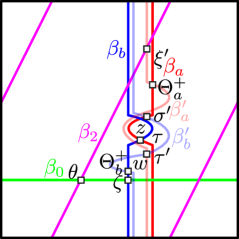

Consider the Heegaard diagram (together with standard translates) given by Figure 6.1, and work over the ring and assign the weight to both basepoints and . Consider the following vertical maps and between the twisted complexes and .
We claim that they are cycles and that and are modulo . Recall that for instance, for , this means that the composition of the vertical maps on the left hand side is the right hand side modulo .
Showing the above is equivalent to the following:
-
•
and are twisted complexes: ,
-
•
: , , ,
-
•
: , , ,
-
•
: , , , modulo
-
•
: , , , modulo
Remark 6.1.
In fact, we can explicitly compute and . All the ’s and ’s vanish, and the ’s are for the unit .
Some of these are easy to verify. Indeed, the ’s, , and vanish because there are no relevant bigons and triangles. The hexagon count vanishes because there are no relevant hexagons that do not contain any basepoints.
To verify the rest, we work in the universal cover of . It will be useful to have names for some right triangles.
Definition 6.2.
Let be the straight, vertical line that is in the middle of and . We abuse notation and label the intersection points as follows: , . Also, let , where . See Figure 6.2.
-
•
Let triangles and , respectively, for be the th right-side up triangle that has vertices and , respectively.
-
•
Let triangles and , respectively, for be the th upside down triangle that has vertices and , respectively.
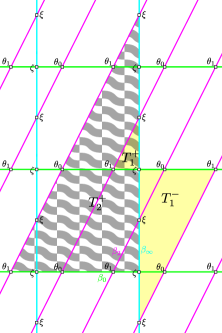

6.1. The ’s vanish
For and , there are two families of triangles that cancel each other. These are related by “rotation by .” In fact, all of the quadrilaterals (and hexagons) that cancel in pairs are also related by “rotation by ” in some sense.
We consider . The two smallest triangles are drawn in the left hand side of Figure 6.3. These have one basepoint, and hence have weight . The next smallest triangles are drawn in Figure 6.5, and they have weight , as they contain five basepoints.
We view these triangles as small perturbations of . (We think of and as being close to each other: the region between them is “small.”) Such triangle or uniquely determines the corresponding triangle that contributes to . For each , there are two of them, one from and one from , and they have weight . Hence they all cancel.


6.2. The ’s vanish
We will write instead of and instead of , etc. since distinguishing them in this subsection is meaningless.
Let us show that , , and vanish. Any quadrilateral that contributes in these quadrilateral count has vertices . There are two families of quadrilaterals with vertices that cancel each other. The two smallest quadrilaterals are drawn in the right hand side of Figure 6.3. These do not have any basepoints, and hence have weight . The next smallest are drawn in Figure 6.6, and they have weight .
We view these quadrilaterals as small perturbations of ’s as in Subsection 6.1. Given a triangle , specifying such a quadrilateral is equivalent to choosing a lift of as vertices of the quadrilateral. For each of and , there is such choices, and there are exactly basepoints for each such quadrilateral. Hence they all cancel.
Computing is slightly more complicated since the quadrilaterals do not need to have as a vertex, but if we work modulo , then they all have as a vertex, and there are exactly two of them, which cancel.
6.3. The ’s are the identity modulo
For the ’s, in all the cases, the Maslov index pentagons are small perturbations of the above quadrilaterals (not every quadrilateral has a small perturbation that contributes to ). In each case, there is exactly one pentagon with vertices and () that does not contain any basepoints. This pentagon is a small perturbation of the top quadrilateral in the right hand side of Figure 6.3. Two of these are drawn in Figure 6.4.
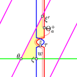


7. Local computation for Claim 5.3

Consider the Heegaard diagram Figure 7.1, and work over the ring and assign the weight to . The circle has a nontrivial local system whose monodromy is given by the oriented arc .
Consider the following vertical maps and between the twisted complexes and .
As in Section 6, we will show that they are cycles and that and are modulo .
As before, this is equivalent to showing the following.
-
•
-
•
,
-
•
,
-
•
, , , modulo
-
•
modulo
We also need to check for Theorem 4.5.
Remark 7.1.
We can explicitly compute and . Indeed, we get and the ’s are where the is the same as in Section 6: .
Similarly, the ’s vanish because there are no bigons, and the vanish because there are no pentagons with Maslov index .
7.1. The ’s vanish
We evaluate the triangle counting maps. Recall Definition 6.2.
We compute , which is the most complicated case, since it is not a priori obvious that the triangles and do not contribute. Recall that .
-
•
The triangle contributes
-
•
The triangle contributes
(note that )
-
•
The triangle contributes some multiple of
and so they all cancel and we get .
The rest vanish as well by direct computation.
7.2. The ’s are the identity

We compute , which is the most complicated case. If we work modulo , then the two small quadrilaterals highlighted in yellow in Figure 7.2 are the only quadrilaterals that contribute. The top one outputs and the bottom one outputs . Hence, they add up to
For the other ’s, there is exactly one quadrilateral that contributes, which gives or .
8. Completing the proof of Theorem 4.3
8.1. A homological -grading
A useful observation that we will repeatedly use is that the following Heegaard datum is -gradable. Compare [MO08, Section 3] and [BL12, Section 5.2].
Proposition 8.1.
Consider the multi-Heegaard diagram given in Figure 4.1, and add any number of standard translates of . Work over and assign the weight to , and to and . Then, this Heegaard datum is -gradable.
Proof.
This is a corollary of Proposition 2.65: the ’s are homologous, and the intersection points are all in torsion -structures. ∎
We let the top -grading elements of and have -grading . Then, the top -grading elements of , , , have -grading , , , , respectively.
We will consider the twisted complex in this graded sense as well, in which case we take .
8.2. An Alexander -splitting
It turns out that the following Heegaard datum with attaching curves and their standard translates is -splittable.

Proposition 8.2.
Consider the multi-Heegaard diagram defined in Section 5, and add any number of standard translates of these attaching curves. Work over and assign the weight to , and to and . Then, this Heegaard datum is -splittable.
Proof.
We check that is even for any cornerless two-chain . Lemma 2.62 and Corollary 2.63 are not directly applicable, but we can reduce the number of cases to check using similar ideas.
Perhaps the most nontrivial special case to check is for the cornerless two-chain in Figure 8.1, whose boundary has exactly one circle with slope . We have , which is even. Given any cornerless two-chain , using the above cornerless two-chain and small cornerless two-chains between two circles which are standard translates of each other, we can reduce it to the case where has no components with slope . Hence, it also does not have any components with slope , and so its boundary only consists of vertical circles and homologically trivial circles. This case follows from an argument similar to that of Lemma 2.62: the two-chain is a sum of cornerless two-chains with two vertices, and we can check these directly. ∎
We let all the generators that we have considered in Section 5 have Alexander -grading . This is indeed possible: there are two things to check. One is that we do not get a contradiction from the maps from Claims 5.2, and the other is that the ’s have Alexander -grading . Consider the intersection point that corresponds to . Then, the former follows from that and . The latter also follows from direct computations.
8.3. Another computation
Let us briefly study the top -grading component of . The top -grading (grading ) generators are , , , and in Figure 8.2. (The intersection points in the free-stabilizing region are not drawn.) The Alexander -grading of is , and the rest are . One can check that, among linear combinations of , , and , the sum is the only nontrivial cycle, regardless of the almost complex structure.
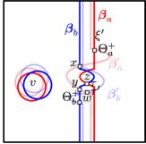
8.4. Independence under variation of the almost complex structure
We show that the statement of Theorem 4.3 is insensitive of the almost complex structure. Let us first check that the maps are invariant. In all the cases, this will follow from that there are no relevant domains with the right Maslov index, which is easy to check, thanks to Proposition 8.1.
The generators , , , and are invariant under changing the almost complex structure, since the chain map induced by changing the almost complex structure preserves both the -grading and the Alexander -grading, and the above generators are the unique nontrivial cycle in the corresponding -grading. Hence, in particular, is preserved under changing the almost complex structure.
Since the top -grading of is and has -grading , the elements and are preserved under changing the almost complex structure.
The maps and are invariant as well. Since the top -grading of is , they are invariant as elements of . Hence, is invariant.
Finally, if we know that and for some choice of almost complex structure, then in any other almost complex structure, we know that they are equal in homology, but since they are in the top -grading, they must be equal.
8.5. Finishing off the proof
We have considered the twisted complexes , , and , and we have defined maps between each consecutive pair in in Sections 5, 6, and 7 (see Remark 5.6). However, we assumed in Claims 5.1 and 5.3 that the underlying almost complex structures are sufficiently stretched. Fortunately, the maps , , and are “invariant” under the -functors defined by changing the almost complex structure since there are no domains that could contribute. Hence, all the twisted complexes that we have considered are invariant as well, and so by applying the -functor, we get pairs of maps between each consecutive pair in , in any almost complex structure. Let and be the compositions of these maps. By Lemma 2.34, Remark 2.35, and Lemma 2.36, these paired with another attaching curve are quasi-isomorphisms. Also note that and have Alexander -grading .
We claim that the top -grading components of and are . Let be another standard translate of . Then, is weakly admissible, and both homologically -gradable and Alexander -splittable. Since
is a quasi-isomorphism and , it cannot strictly lower the -grading. Since the top -grading of is , the -grading part of is nontrivial, and so it must be , as it is the unique cycle in -grading and Alexander -grading . We similarly get that .
Now, we claim that and are the top -grading components of and , respectively. Since the top -grading of is and the top -grading of is , the top -grading and Alexander -grading component of is generated by and , and is the unique nontrivial cycle. Since the top grading component of is a cycle, it must be . Similarly, is the top grading component of .
Since and have -grading and the -grading part of and are both , we get that and .
9. Computation for planar links
In this section, we compute the band maps for planar links. First, let us compute the unoriented link Floer homology of unlinks.
Proposition 9.1.
Let be a balled link in , where the underlying link is an unlink. Let the link baseballs correspond to variables . Then, the unoriented link Floer homology of the balled link is canonically isomorphic to
over the coefficient ring, hence in particular over .
Proof.
Iterate Proposition 2.41. ∎
Note that as an -module, the homology is freely generated and has rank .
Although this is tangential to the rest of this section, we compute non-orientable band maps between unlinks: they agree with Khovanov homology.
Theorem 9.2.
Non-orientable band maps between unlinks in are zero.
Proof.
Let be a band between two unlinks with components. We use the infinity version of the unoriented skein exact triangle: complete to an unoriented skein triple; let be the third link. Then has components. As -vector spaces, has rank , and has rank by Proposition 3.6. Hence, the band map
is zero. Since the map is injective, the map on the minus version is also zero. ∎
The band maps for planar links in unoriented link Floer homology coincide with that in equivariant Khovanov homology given by the Lee deformation.
Theorem 9.3.
Let be a merge band from to where and are balled unlinks in . Assume that the band and the underlying links of and (ignoring the baseballs) all lie in . Without loss of generality, assume that the coefficient ring for is , that the band intersects the link components with link baseballs that correspond to and , and that the baseball that corresponds to becomes a free baseball for the link . Let , and consider and as modules over , freely generated by and , respectively.
-
•
The merge band map for is the -linear map given by
-
•
The split band map for the dual band is the -linear map given by
The corresponding statements for the hat and infinity versions follow immediately. The proof of Theorem 9.3 occupies the remainder of this section.
A Heegaard datum for split and merge band maps between planar links with and components can be obtained by successively free link stabilizing such a Heegaard datum for . Hence, Theorem 9.3 follows from the computation for , together with Propositions 2.39 and 2.41.
Consider the multi-Heegaard diagram in Figure 9.1, and recall the maps from Theorem 4.3. Work over and assign the weight to , and to and . Then, and are the split and merge band maps, respectively, between planar links with one and two components.

We will not use and directly to compute the band maps. Proposition 2.65 also shows that the Heegaard datum with Heegaard diagram
is -gradable. Hence, the merge and split band maps are the top -grading components of the compositions of
respectively, which are induced by the three maps discussed in Section 5 (see Remark 5.6). Indeed, the band maps must be the top grading components since the merge and split band maps cannot be zero, because of the exact triangle (it is also possible to compute the gradings directly).
Remark 9.4.
As the band maps are -linear and homogeneous, the skein exact triangle narrows the maps down to two possibilities:
we will show that it is indeed the latter.
9.1. A local computation
Figure 9.2 is key to computing the band maps.

Proposition 9.5.
Consider the Heegaard diagram given in Figure 9.2. Work over and assign the weight to both and . Let us write . The chain complex is freely generated by over , and the only nontrivial differential is . Hence, we get
after identifying and with their homology classes. Furthermore, the maps and induced by and , respectively, are cycles and we have
-
•
;
-
•
9.2. Split bands

To compute , we consider another curve as in Figure 9.3 and compute the maps paired with instead. Then, we use the following commutative diagram
We can compute every chain complex that arises as vertices in the above diagram, and we can compute all the maps except .
9.2.1. The homology groups
Let us first study the relevant homology groups. We remark that the -category that consists of and their standard translates (in fact, , is a standard translate of , , respectively) is both -gradable and -splittable.
The Heegaard diagram is a free-stabilization of the Heegaard diagram from Figure 9.2. Hence we identify (as -modules, where acts as , and so equivalently as -modules)
where by and , we really mean their free-stabilizations and from Subsection 2.6. In fact, these are canonical since is the top -grading generator and where is the homology class of the vertical circle in Figure 9.3 and is the -action from [OS04c, Subsection 4.2.5] (see [Zem15, Subsection 5.3]). Since and are obtained by handsliding and , respectively, there are canonical isomorphisms from to and , and we use to denote the image of these generators under the canonical isomorphisms.
Similarly, identify
This is also canonical since and are the top grading generators in their respective Alexander grading or --structure. We similarly write and for the image of these elements under the canonical isomorphisms from to groups canonically isomorphic to it. We also identify
Also, let be the top grading generator of .
We discuss and related groups in the next subsubsection.
9.2.2. The maps and
Although the homology groups and ; and and are canonically isomorphic via and , respectively, it is not a priori clear whether and are. Indeed, the isomorphism is given by the following dashed map on homology.
In other words, this is the case where we know that the outer square commutes up to homotopy, but we really care which homotopy we chose.
Fortunately, the chain complex has a nice splitting into two sub chain complexes:
where is generated, as an -module, by the intersection points whose --structure is the same as and is generated by the rest. Let us call this the -splitting for now474747This is basically the -splitting, but has grading in this case..
Since we only consider , there is also a -grading. Shift the -grading of or appropriately such that is a twisted complex in the graded sense. Then, there is a canonical splitting, i.e. an -linear isomorphism
where and are homogeneous with respect to both the -grading and the -splitting, and and lie in different -summands. In particular, with respect to the splitting (as modules)
we can assume that for some , and . By abuse of notation, we denote and as and , respectively.
Use the same notation for . This is now justified, since the isomorphism preserves both the -grading and the -splitting, and is -linear. Hence, the map sends to and to . Similarly, the isomorphism sends to and to .
Remark 9.7.
The chain complex is simpler if the curve in Figure 9.2 had slope instead of . However, it would be harder to compute the maps considered in this subsection.
9.2.3. The maps and
We pinch the neck and use Proposition 9.5, which gives the following:
-
•
;
-
•
.
9.2.4. The split band map
Putting all these together, we get that the composite is
and hence the split band map is
Remark 9.8.
We could have worked with the maps discussed in Remark 5.6 that are morally homotopy inverses of each other. In this case, the composite is indeed just
9.3. Merge bands
One way to compute the merge band map is to argue as in Subsection 9.2. There is a simpler way: the merge band map for planar links can be computed using the same triple Heegaard diagram as the split band map, by composing with different algebraic maps as in Definition 3.21.

Indeed, consider Figure 9.4. Let and . Assign the weight to both and , and let over any ring. We have computed the split band map, which is
Identifying
the split band map is -linear, and is given by . Hence, as the map
is -linear, it is determined by . Now we can compute the merge band map: it is
which is the -linear map given by
which is what we wanted.
References
- [Bha23] Deeparaj Bhat, Surgery exact triangles in instanton theory, arXiv preprint arXiv:2311.04242 (2023).
- [BL12] John A. Baldwin and Adam Simon Levine, A combinatorial spanning tree model for knot Floer homology, Adv. Math. 231 (2012), no. 3-4, 1886–1939. MR 2964628
- [BLS17] John A. Baldwin, Adam Simon Levine, and Sucharit Sarkar, Khovanov homology and knot Floer homology for pointed links, J. Knot Theory Ramifications 26 (2017), no. 2, 1740004, 49. MR 3604486
- [Dow24] Nathan Dowlin, A spectral sequence from Khovanov homology to knot Floer homology, J. Amer. Math. Soc. 37 (2024), no. 4, 951–1010. MR 4777638
- [Fan17] Haofei Fan, Unoriented cobordism maps on link Floer homology, arXiv preprint arXiv:1711.07110 (2017).
- [Flo88] Andreas Floer, An instanton-invariant for 3-manifolds, Communications in mathematical physics 118 (1988), 215–240.
- [HHSZ20] Kristen Hendricks, Jennifer Hom, Matthew Stoffregen, and Ian Zemke, Surgery exact triangles in involutive Heegaard Floer homology, arXiv preprint arXiv:2011.00113 (2020).
- [HHSZ24] by same author, Naturality and functoriality in involutive Heegaard Floer homology, Quantum Topology (2024).
- [HM17] Kristen Hendricks and Ciprian Manolescu, Involutive Heegaard Floer homology, Duke Math. J. 166 (2017), no. 7, 1211–1299. MR 3649355
- [JTZ21] András Juhász, Dylan Thurston, and Ian Zemke, Naturality and mapping class groups in Heegard Floer homology, Mem. Amer. Math. Soc. 273 (2021), no. 1338, v+174. MR 4337438
- [Juh06] András Juhász, Holomorphic discs and sutured manifolds, Algebr. Geom. Topol. 6 (2006), 1429–1457. MR 2253454
- [JZ24] András Juhász and Ian Zemke, Stabilization distance bounds from link Floer homology, Journal of Topology 17 (2024), no. 2, e12338.
- [Kho00] Mikhail Khovanov, A categorification of the Jones polynomial, Duke Math. J. 101 (2000), no. 3, 359–426. MR 1740682
- [KM10] Peter Kronheimer and Tomasz Mrowka, Knots, sutures, and excision, J. Differential Geom. 84 (2010), no. 2, 301–364. MR 2652464
- [KM11] P. B. Kronheimer and T. S. Mrowka, Khovanov homology is an unknot-detector, Publ. Math. Inst. Hautes Études Sci. (2011), no. 113, 97–208. MR 2805599
- [Lee05] Eun Soo Lee, An endomorphism of the Khovanov invariant, Adv. Math. 197 (2005), no. 2, 554–586. MR 2173845
- [Lip06] Robert Lipshitz, A cylindrical reformulation of Heegaard Floer homology, Geom. Topol. 10 (2006), 955–1096, [Paging previously given as 955–1097]. MR 2240908
- [LOT16] Robert Lipshitz, Peter S. Ozsváth, and Dylan P. Thurston, Bordered Floer homology and the spectral sequence of a branched double cover II: the spectral sequences agree, J. Topol. 9 (2016), no. 2, 607–686. MR 3509974
- [LOT18] Robert Lipshitz, Peter S. Ozsvath, and Dylan P. Thurston, Bordered Heegaard Floer homology, Mem. Amer. Math. Soc. 254 (2018), no. 1216, viii+279. MR 3827056
- [LS22] Robert Lipshitz and Sucharit Sarkar, A mixed invariant of nonorientable surfaces in equivariant Khovanov homology, Trans. Amer. Math. Soc. 375 (2022), no. 12, 8807–8849. MR 4504654
- [LY22] Zhenkun Li and Fan Ye, Instanton Floer homology, sutures, and Heegaard diagrams, J. Topol. 15 (2022), no. 1, 39–107. MR 4407491
- [LY24] Zhenkun Li and Fan Ye, 2-torsion in instanton Floer homology, 2024.
- [Man07] Ciprian Manolescu, An unoriented skein exact triangle for knot Floer homology, Math. Res. Lett. 14 (2007), no. 5, 839–852. MR 2350128
- [MO08] Ciprian Manolescu and Peter Ozsváth, On the Khovanov and knot Floer homologies of quasi-alternating links, Proceedings of Gökova Geometry-Topology Conference 2007, Gökova Geometry/Topology Conference (GGT), Gökova, 2008, pp. 60–81. MR 2509750
- [MO10] Ciprian Manolescu and Peter Ozsváth, Heegaard Floer homology and integer surgeries on links, arXiv preprint arXiv:1011.1317 (2010).
- [Nah] Gheehyun Nahm, Rational surgery exact triangles in Heegaard Floer homology, In preparation.
- [OS04a] Peter Ozsváth and Zoltán Szabó, Holomorphic disks and knot invariants, Adv. Math. 186 (2004), no. 1, 58–116. MR 2065507
- [OS04b] by same author, Holomorphic disks and three-manifold invariants: properties and applications, Ann. of Math. (2) 159 (2004), no. 3, 1159–1245. MR 2113020
- [OS04c] by same author, Holomorphic disks and topological invariants for closed three-manifolds, Ann. of Math. (2) 159 (2004), no. 3, 1027–1158. MR 2113019
- [OS05] by same author, On the Heegaard Floer homology of branched double-covers, Adv. Math. 194 (2005), no. 1, 1–33. MR 2141852
- [OS06] by same author, Holomorphic triangles and invariants for smooth four-manifolds, Adv. Math. 202 (2006), no. 2, 326–400. MR 2222356
- [OS08a] Peter Ozsváth and Zoltán Szabó, Holomorphic disks, link invariants and the multi-variable Alexander polynomial, Algebr. Geom. Topol. 8 (2008), no. 2, 615–692. MR 2443092
- [OS08b] Peter S. Ozsváth and Zoltán Szabó, Knot Floer homology and integer surgeries, Algebr. Geom. Topol. 8 (2008), no. 1, 101–153. MR 2377279
- [OS09] Peter Ozsváth and Zoltán Szabó, A cube of resolutions for knot Floer homology, J. Topol. 2 (2009), no. 4, 865–910. MR 2574747
- [OSS15] Peter S. Ozsváth, András I. Stipsicz, and Zoltán Szabó, Grid homology for knots and links, Mathematical Surveys and Monographs, vol. 208, American Mathematical Society, Providence, RI, 2015. MR 3381987
- [OSS17a] by same author, Concordance homomorphisms from knot Floer homology, Adv. Math. 315 (2017), 366–426. MR 3667589
- [OSS17b] Peter S. Ozsváth, András I. Stipsicz, and Zoltán Szabó, Unoriented knot Floer homology and the unoriented four-ball genus, Int. Math. Res. Not. IMRN (2017), no. 17, 5137–5181. MR 3694597
- [Ras03] Jacob Andrew Rasmussen, Floer homology and knot complements, ProQuest LLC, Ann Arbor, MI, 2003, Thesis (Ph.D.)–Harvard University. MR 2704683
- [Ras05] Jacob Rasmussen, Knot polynomials and knot homologies, Geometry and topology of manifolds, Fields Inst. Commun., vol. 47, Amer. Math. Soc., Providence, RI, 2005, pp. 261–280. MR 2189938
- [Sar11] Sucharit Sarkar, Maslov index formulas for Whitney -gons, J. Symplectic Geom. 9 (2011), no. 2, 251–270. MR 2811652
- [Sar15] by same author, Moving basepoints and the induced automorphisms of link Floer homology, Algebr. Geom. Topol. 15 (2015), no. 5, 2479–2515. MR 3426686
- [Sei08] Paul Seidel, Fukaya categories and Picard-Lefschetz theory, Zurich Lectures in Advanced Mathematics, European Mathematical Society (EMS), Zürich, 2008. MR 2441780
- [Ye23] Fan Ye, 2-torsions in singular instanton homology, 2023, https://www.youtube.com/watch?v=Z3ltYNI61a0.
- [Zem15] Ian Zemke, Graph cobordisms and Heegaard Floer homology, arXiv preprint arXiv:1512.01184 (2015).
- [Zem17] by same author, Quasistabilization and basepoint moving maps in link Floer homology, Algebr. Geom. Topol. 17 (2017), no. 6, 3461–3518. MR 3709653
- [Zem19] by same author, Link cobordisms and functoriality in link Floer homology, J. Topol. 12 (2019), no. 1, 94–220. MR 3905679
- [Zem21a] by same author, Bordered manifolds with torus boundary and the link surgery formula, arXiv preprint arXiv:2109.11520 (2021).
- [Zem21b] by same author, Duality and mapping tori in Heegaard Floer homology, J. Topol. 14 (2021), no. 3, 1027–1112. MR 4503956
- [Zem23] by same author, A general Heegaard Floer surgery formula, arXiv preprint arXiv:2308.15658 (2023).