The R Package WMAP: Tools for Causal Meta-Analysis by Integrating Multiple Observational Studies

Abstract

Integrating multiple observational studies for meta-analysis has sparked much interest. The presented R package WMAP (Weighted Meta-Analysis with Pseudo-Population) (Guha et al., 2024) addresses a critical gap in the implementation of integrative weighting approaches for multiple observational studies and causal inferences about various groups of subjects, such as disease subtypes. The package features three weighting approaches, each representing a special case of the unified weighting framework introduced by Guha and Li (2024), which includes an extension of inverse probability weights for data integration settings. It performs meta-analysis on user-inputted datasets as follows: (i) it first estimates the propensity scores for study-group combinations, calculates subject balancing weights, and determines the effective sample size (ESS) for a user-specified weighting method; and (ii) it then estimates various features of multiple counterfactual group outcomes, such as group medians and differences in group means for the mRNA expression of eight genes. Additionally, bootstrap variability estimates are provided. Among the implemented weighting methods, we highlight the FLEXible, Optimized, and Realistic (FLEXOR) method, which is specifically designed to maximize the ESS within the unified framework. The use of the software is illustrated by simulations as well as a multi-site breast cancer study conducted in seven medical centers.

Keywords: pseudo-population; retrospective cohort; unconfounded comparison; weighting.

1 Introduction

When analyzing observational studies, balancing covariates is a crucial step for unconfounded causal comparisons of group potential outcomes (Robins and Rotnitzky, 1995; Rubin, 2007). In diverse research areas, the observed or underlying sampling populations of observational studies, in addition to being unbalanced with respect to the group-specific covariates, are invariably very different from the larger natural population of interest. It is therefore necessary to utilize covariate-balancing techniques like weighting or matching (Lunceford and Davidian, 2004). Weighting methods in observational studies with two subject groups rely on the propensity score, and overwhelmingly, utilize inverse probability weights (IPWs) to achieve covariate balance (Rosenbaum and Rubin, 1983; Li and Li, 2019). However, IPW estimators of group differences are often unstable if one of more subjects have extreme PS values (Li and Li, 2019). Consequently, variations of IPWs motivated by truncated subpopulations have been developed (e.g., Crump et al., 2006; Li and Greene, 2013).

Most weighting methods in the literature provide valid inferences for a covariate-balanced pseudo-population that differs from the larger, natural population of interest for which no random samples are available. For example, IPWs correspond to a so-called combined pseudo-population. Overlap weights minimize the asymptotic variance of the weighted average treatment effect for the overlap pseudo-population (Li et al., 2018). For single observational studies with two or more groups, generalized overlap weights minimize the sum of asymptotic variances of weighted estimators of pairwise group differences (Li and Li, 2019). These approaches have the following shortcomings: (i) they are optimal for restricted outcome types and estimands (typically, contrasts of group means) under theoretical conditions that may not be satisfied in practice; furthermore, the study goals may involve very different estimands than the group mean contrasts of counterfactual outcomes (e.g., percentiles, medians, or pairwise correlations of multivariate group responses) and various unplanned estimands; (ii) they are not appropriate for the meta-analysis of multiple observational studies with each study comprising more than two subject groups.

Motivated by these challenges, Guha and Li (2024) extended the propensity score to the multiple propensity score (MPS). Further, they proposed a general family of pseudo-populations and balancing weights that facilitate the integrative analyses and causal inferences of diverse functionals of group-specific potential outcomes. This unified framework generalizes the aforementioned weighting methods to the meta-analysis of multiple studies with multiple groups. Specifically, as explained in Section 2, IPWs and overlap weights (Li et al., 2018; Li and Li, 2019) are extended to the integrative combined (IC) and integrative generalized overlap (IGO) weights, respectively. Furthermore, by optimizing the effective sample size (ESS) of pseudo-populations within this rich family, Guha and Li (2024) invented the so-called FLEXible, Optimized, and Realistic (FLEXOR) weights and studied the properties of these estimand-agnostic and efficient weighted estimators for quantitative, categorical, or multivariate outcomes. The substantial benefits of FLEXOR relative to extensions of existing weighting methods such as IC and IGO are demonstrated using simulated and TCGA cancer datsets in that paper. We have developed an R package, WMAP, to implement the three weighting methods (Guha et al., 2024). The approach formulated by Guha and Li (2024) fills a methodological gap by pioneering a principled, estimand-agnostic integrative causal approach capable of accommodating multiple studies with multiple groups, a structure frequently encountered in contemporary integrative research. To our knowledge, the present R package is the first implementation of such a method.

The paper is structured as follows. Section 2 reviews the weighting methodology and two-stage inference procedure of the FLEXOR approach. Section 3 conducts simulations by using the package. Section 4 presents the meta-analysis of multiple breast cancer studies as a case study, describing the general workflow, illustrating the inferential procedure and presenting biologically meaningful results. Section 6 discusses future directions.

2 Methodology

In a large population of interest, suppose there are $K$ groups of patients about whom nothing is known a priori besides the disease prevalences available from registries. The meta-analysis integrates $J$ retrospective cohorts or studies with each study recording the covariates for each subject. For participant $i$, let $S_{i}$ denote their observational study, $Z_{i}$ denote their group, and $\mathbf{X}_{i}\in\mathcal{X}\subset\mathcal{R}^{p}$ denote their covariate vector, and vector of $L$ outcomes by $\mathbf{Y}_{i}\in\mathcal{R}^{L}$. Writing the $z$th group’s counterfactual outcome vector (i.e., the outcome if the $i$th subject had belonged to group $z$) by $\mathbf{Y}_{i}^{(z)}=(Y_{i1}^{(z)},\ldots,Y_{iL}^{(z)})^{\prime}$, the observed outcome is then $\mathbf{Y}_{i}=\mathbf{Y}_{i}^{(Z_{i})}$. We further assume that (a) $J$ and $K$ are not large, (b) a subject belongs to just one observational study, and (c) subjects belonging to all $K$ groups are observed in every study.

If the subject labels are not meaningful, then $(S_{i},Z_{i},\mathbf{X}_{i},\mathbf{Y}_{i})$ may be regarded as i.i.d. samples from an observed population with density $p_{+}[S,Z,\mathbf{X},\mathbf{Y}]$, where $p_{+}[\cdot]$ represents observed population distributions or densities with respect a dominating measure. Generalizing the assumptions of Rubin (2007) and Imbens (2000), we assume: (I) Stable unit treatment value assumption (SUTVA): Conditional on the covariates, the study and group to which a subject belongs has no effect on their potential outcomes, and every version of grouping would lead to the same potential outcomes; (II) Study-specific unconfoundedness: Given study $S_{i}$ and covariate $\mathbf{X}_{i}$, group $Z_{i}$ is statistically independent of $\mathbf{Y}_{i}^{(1)},\ldots,\mathbf{Y}_{i}^{(K)}$, i.e., $p_{+}[\mathbf{Y}^{(z)}\mid S,Z,\mathbf{X}]=p_{+}[\mathbf{Y}^{(z)}\mid S,\mathbf{X}]$; and (III) Positivity: $p_{+}[S=z,Z=z,\mathbf{X}=\mathbf{x}]>0$ for all $(s,z,\mathbf{x})$. Under these conditions, the presented WMAP package performs a two-stage analysis: Stage 1 computes weights to integrate multiple studies, and Stage 2 uses these weights to infer group counterfactual outcomes.

2.1 Stage 1: Outcome-free sample weights

For the purpose of meta-analysis, we generalize the propensity score (e.g., Rosenbaum and Rubin, 1983) to the multiple propensity score (MPS) of study-group memberships belonging to $\Sigma=$ $\{1,\ldots,J\}\times\{1,\ldots,K\}.$ For $\mathbf{x}\in\mathcal{X}$, the MPS is defined as

$$\delta_{sz}(\mathbf{x})=p_{+}\bigl{[}S=s,Z=z\mid\mathbf{X}=\mathbf{x}\bigr{]}\quad\text{for $(s,z)\in\Sigma$. }$$ (1)

In observational studies, the unknown MPS is estimated by regressing the factor variable $(S_{i},Z_{i})$ on $\mathbf{x}_{i}$ for the $N$ subjects using parametric or nonparametric regression techniques. Using MPS, we can derive subject-specific balancing weights that redistribute, and thereby, transform the density of the (unbalanced) observed population to a covariate-balanced pseudo-population (Guha and Li, 2024) in which a patient’s study, group and covariates are mutually independent by design:

$$p\bigl{[}S=s,Z=z,\mathbf{X}=\mathbf{x}\bigr{]}=\gamma_{s}\,\theta_{z}\,f_{\boldsymbol{\gamma},\boldsymbol{\theta}}(\mathbf{x}),\quad\text{for $(s,z,\mathbf{x})\in\Sigma\times\mathcal{X}$,}$$ (2)

where $p[\cdot]$ denotes distributions or densities with respect to the pseudo-population, and which relies on probability vector $\boldsymbol{\gamma}=(\gamma_{1},\ldots,\gamma_{J})$ quantifying the study relative masses, relative group prevalences $\boldsymbol{\theta}=(\theta_{1},\ldots,\theta_{K})$, and pseudo-population covariate density $f_{\boldsymbol{\gamma},\boldsymbol{\theta}}(\mathbf{x})$. In some investigations, it is possible to specify group prevalence $\boldsymbol{\theta}$ to match the group prevalence of the natural population. However, reasonable choices of $\boldsymbol{\gamma}$ are often unknown because they are primarily determined by the study designs and unknown factors influencing cohort participation. If any component of $\boldsymbol{\gamma}$ or $\boldsymbol{\theta}$ is unknown, we can optimize the pseudo-population in later steps with respect to these quantities.

Let the marginal observed covariate density be denoted by $f_{+}(\mathbf{x})$, $\mathbf{x}\in\mathcal{X}$. Then, there exists a tilting function (e.g., Li et al., 2018), $\eta_{\boldsymbol{\gamma},\boldsymbol{\theta}}$, such that $f_{\boldsymbol{\gamma},\boldsymbol{\theta}}(\mathbf{x})\propto\eta_{\boldsymbol{\gamma},\boldsymbol{\theta}}(\mathbf{x})f_{+}(\mathbf{x})$, implying that $f_{\boldsymbol{\gamma},\boldsymbol{\theta}}(\mathbf{x})=\eta_{\boldsymbol{\gamma},\boldsymbol{\theta}}(\mathbf{x})f_{+}(\mathbf{x})/\mathbb{E}_{+}[\eta_{\boldsymbol{\gamma},\boldsymbol{\theta}}(\mathbf{X})]$, where $\mathbb{E}_{+}(\cdot)$ denotes expectations under the observed distribution in which $\mathbf{X}\sim f_{+}$. This gives an alternative characterization of pseudo-populations relying on tilting functions instead of covariate densities. In particular, with $\mathcal{S}_{J}$ denoting the unit simplex in $\mathcal{R}^{J}$, different $\boldsymbol{\gamma}\in\mathcal{S}_{J}$, $\boldsymbol{\theta}\in\mathcal{S}_{K}$, and tilting function $\eta_{\boldsymbol{\gamma},\boldsymbol{\theta}}$ result in different pseudo-populations belonging to family (2) as natural meta-analytical extensions of existing weighting methods for single studies. For example, equally weighted studies and groups, along with tilting function $\eta_{\boldsymbol{\gamma},\boldsymbol{\theta}}(\mathbf{x})\propto 1$ and $\eta_{\boldsymbol{\gamma},\boldsymbol{\theta}}(\mathbf{x})=1/\sum_{s}\sum_{z}\delta_{sz}^{-1}(\mathbf{x})$, respectively, extends the combined (Li et al., 2018) and generalized overlap (Li and Li, 2019) pseudo-populations to the integrative combined (IC) and integrative generalized overlap (IGO) pseudo-populations, respectively.

For more generality and efficiency, we define a (multi-study) balancing weight as the ratio of pseudo-population and observed population densities (Guha and Li, 2024) . For $(s,z,\mathbf{x})\in\Sigma\times\mathcal{X}$, balancing weight

$$\rho_{\boldsymbol{\gamma},\boldsymbol{\theta}}(s,z,\mathbf{x})=\frac{\gamma_{s}\,\theta_{z}\,\eta_{\boldsymbol{\gamma},\boldsymbol{\theta}}(\mathbf{x})}{\delta_{sz}(\mathbf{x})\,\mathbb{E}_{+}[\eta_{\boldsymbol{\gamma},\boldsymbol{\theta}}(\mathbf{X})]}.$$ (3)

redistributes the observed distribution’s density to equal the pseudo-population’s density . The unnormalized sample weights, $\tilde{\rho}_{i}=$ $\gamma_{s_{i}}\theta_{z_{i}}\eta_{\boldsymbol{\gamma},\boldsymbol{\theta}}(\mathbf{x}_{i})/\delta_{s_{i}z_{i}}(\mathbf{x}_{i})$, are later used to evaluate unconfounded weighted estimators of various counterfactual outcome features in the pseudo-population. The empirically normalized balancing weight is computed from the $N$ unnormalized sample weights as $\rho_{i}=\tilde{\rho}_{i}/\sum_{u=1}^{N}\tilde{\rho}_{u}$ and is normalized to have sample mean 1.

A widely used, estimand-agnostic measure of a weighting method’s inferential accuracy is the effective sample size (ESS) (e.g., McCaffrey et al., 2013), $\mathcal{Q}(\boldsymbol{\gamma},\boldsymbol{\theta},\eta_{\boldsymbol{\gamma},\boldsymbol{\theta}})=N/\bigl{[}1+\text{Var}_{+}\bigl{\{}\rho_{\boldsymbol{\gamma},\boldsymbol{\theta}}(S,Z,\mathbf{X})\bigr{\}}\bigr{]}=N/\mathbb{E}_{+}\bigl{\{}\rho_{\boldsymbol{\gamma},\boldsymbol{\theta}}^{2}(S,Z,\mathbf{X})\bigr{\}}$, where $\mathbb{E}[\cdot]$ and $\text{Var}[\cdot]$ respectively denote expectations and variances with respect to the pseudo-population. When $N$ is large, the ESS is reliably estimated by the sample ESS, $\tilde{\mathcal{Q}}(\boldsymbol{\gamma},\boldsymbol{\theta},\eta_{\boldsymbol{\gamma},\boldsymbol{\theta}})=N^{2}/\sum_{i=1}^{N}\rho_{i}^{2}$, using the empirically normalized weights.

We define the FLEXOR pseudo-population as a member of family (2) maximizing ESS subject to any investigator-imposed restrictions that $\boldsymbol{\gamma}$ and $\boldsymbol{\theta}$ must belong to $\Upsilon\subset\mathcal{S}_{J}\times\mathcal{S}_{K}$ (Guha and Li, 2024). If the FLEXOR pseudo-population is identified by $(\breve{\boldsymbol{\gamma}},\breve{\boldsymbol{\theta}},\breve{\eta}_{\breve{\boldsymbol{\gamma}},\breve{\boldsymbol{\theta}}})$, then

$$\mathcal{Q}(\breve{\boldsymbol{\gamma}},\breve{\boldsymbol{\theta}},\breve{\eta}_{\breve{\boldsymbol{\gamma}},\breve{\boldsymbol{\theta}}})=\sup_{(\boldsymbol{\gamma},\boldsymbol{\theta})\in\Upsilon}\sup_{\eta_{\boldsymbol{\gamma},\boldsymbol{\theta}}}\mathcal{Q}(\boldsymbol{\gamma},\boldsymbol{\theta},\eta_{\boldsymbol{\gamma},\boldsymbol{\theta}}).$$

An iterative procedure for estimating FLEXOR pseudo-population

Initializing $(\boldsymbol{\gamma},\boldsymbol{\theta})\in\Upsilon$, we perform the following steps iteratively until the sample ESS converges. The converged pseudo-population with optimized sample ESS estimates the FLEXOR pseudo-population.

• With the parameters $(\boldsymbol{\gamma},\boldsymbol{\theta})$ held fixed, maximize the sample ESS $\tilde{\mathcal{Q}}(\boldsymbol{\gamma},\boldsymbol{\theta},\eta_{\boldsymbol{\gamma},\boldsymbol{\theta}})$ over all tilting functions to obtain the best fixed-$(\boldsymbol{\gamma},\boldsymbol{\theta})$ pseudo-population represented by $(\boldsymbol{\gamma},\boldsymbol{\theta},\breve{\eta}_{\boldsymbol{\gamma},\boldsymbol{\theta}})$. The analytical form of $\breve{\eta}_{\boldsymbol{\gamma},\boldsymbol{\theta}}$ for the theoretical ESS is given by Theorem 1 of Guha and Li (2024):

  $$\breve{\eta}_{\boldsymbol{\gamma},\boldsymbol{\theta}}(\mathbf{x})=\biggl{(}\sum_{s=1}^{J}\sum_{z=1}^{K}\frac{\gamma_{s}^{2}\theta_{z}^{2}}{\delta_{sz}(\mathbf{x})}\biggr{)}^{-1},\quad\text{ $\mathbf{x}\in\mathcal{X}$.}$$

  This pseudo-population’s balancing weights (3) are uniformly bounded over $(s,z,\mathbf{x})\in\Sigma\times\mathcal{X}$. Tilting function $\breve{\eta}_{\boldsymbol{\gamma},\boldsymbol{\theta}}(\mathbf{x})$ de-emphasizes covariate regions where $\delta_{sz}(\mathbf{x})$ is nearly 0 for some $(s,z)\in\Sigma$. At the same time, it promotes covariate regions where the group propensities, $\delta_{z}=\sum_{s=1}^{K}\delta_{sz}(\mathbf{x})$, match group proportion $\theta_{z}$ for every $z=1,\ldots,K$. Set function $\eta=\breve{\eta}_{\boldsymbol{\gamma},\boldsymbol{\theta}}$.

• With tilting function $\eta$ held fixed, maximize the sample ESS $\tilde{\mathcal{Q}}(\boldsymbol{\gamma},\boldsymbol{\theta},\eta)$ over all parameters $(\boldsymbol{\gamma},\boldsymbol{\theta})\in\Upsilon$ to obtain the best fixed-$\eta$ pseudo-population represented by $(\tilde{\boldsymbol{\gamma}},\tilde{\boldsymbol{\theta}},\eta)$. The numerical maximization can be performed using implementations of Gauss-Seidel or Jacobi algorithms. Set $(\boldsymbol{\gamma},\boldsymbol{\theta})=(\tilde{\boldsymbol{\gamma}},\tilde{\boldsymbol{\theta}})$.

The WMAP package includes a function, balancing.weights(), that estimates the MPS and calculates the normalized balancing weights of the $N$ subjects and sample ESS for a user-specified pseudo-population. The required pseudo-population is specified by the user through the argument method, which can be “FLEXOR”, “IC”, or “IGO.” If method="FLEXOR", the iterative procedure, as outlined above, is implemented starting from different initial values to estimate the FLEXOR pseudo-population.

2.2 Stage 2: Unconfounded inferences of group counterfactual outcomes

The theoretical properties (e.g., asymptotic variances) of multivariate weighted estimators of wide-ranging group-level features of the outcomes have been thoroughly investigated (Guha and Li, 2024). We summarize here some special applications of the methodology relevant to the WMAP package implementation. Using univariate outcomes ($L=1$), suppose the potential outcome vectors $Y^{(1)},\ldots,$ $Y^{(K)}$ have common support, $\mathcal{Y}\subset\mathcal{R}$. We assume identical conditional distributions: $p[Y^{(z)}\mid S,Z,\mathbf{X}]=p_{+}[Y^{(z)}\mid S,Z,\mathbf{X}]$ for $z=1,\ldots,K$, guaranteeing that the SUTVA, unconfoundedness, and positivity assumptions for the observed population hold for the pseudo-population. Since the pseudo-population has balanced covariates by design, this implies that $p[Y\mid Z=z]=p[Y^{(z)}]$, paving the way for weighted estimators of potential outcome features for the FLEXOR, IGO, and IC pseudo-populations.

Let $\Phi_{1},\ldots,\Phi_{M}$ be real-valued functions having domain $\mathcal{Y}$. We wish to infer pseudo-population means of transformed potential outcomes, $\mathbb{E}[\Phi_{1}(Y^{(z)})],\ldots,\mathbb{E}[\Phi_{M}(Y^{(z)})]$ for $z=1,\ldots,K$. Appropriate choices of $\Phi_{m}$ correspond to pseudo-population inferences about group-specific marginal means, medians, variances, and CDFs of potential outcome components. Equivalently, writing $\mathbf{\Phi}(Y^{(z)})=\bigl{(}\Phi_{1}(Y^{(z)}),\ldots,\Phi_{M}(Y^{(z)})\bigr{)}^{\prime}\in\mathcal{R}^{M}$, let $\boldsymbol{\lambda}^{(z)}=$ $\mathbb{E}[\mathbf{\Phi}(Y^{(z)})]$. For real-valued functions $\psi$ with domain $\mathcal{R}^{M}$, we wish to estimate $\psi(\boldsymbol{\lambda}^{(z)})$.

For example, define $\Phi_{1}(Y^{(z)})=Y^{(z)}$ and $\Phi_{2}(Y^{(z)})=(Y^{(z)})^{2}$. Then $\psi(t_{1},t_{2})=t_{1}$, we obtain the pseudo-population mean in the $z$th group. Similarly, $\psi(t_{1},t_{2})=\sqrt{t_{2}-t_{1}^{2}}$ gives the pseudo-population standard deviation in the $z$th group. For a second example, let $y_{1},\ldots,y_{M}$ be a fine grid of prespecified points in the support $\mathcal{Y}$ and $\Phi_{m}(Y^{(z)})=\mathcal{I}(Y^{(z)}\leq y_{m})$. For $\psi(t_{1},\ldots,t_{M})=t_{m}$, the pseudo-population CDF of $Y^{(z)}$ evaluated at $y_{m}$ equals $\psi(\boldsymbol{\lambda}^{(z)})$. Similarly, for $\psi(t_{1},\ldots,t_{M})=t_{m^{*}}$ where $m^{*}=\arg\min_{m}|t_{m}-0.5|$, the approximate median of $Y_{1}^{(z)}$ is given by $\psi(\boldsymbol{\lambda}^{(z)})$.

Using the normalized weights $\rho_{1},\ldots,\rho_{N}$, a weighted estimator of mean vector $\boldsymbol{\lambda}^{(z)}$ is

$$\mathbf{\bar{\Phi}}_{z}=\frac{\sum_{i=1}^{N}\rho_{i}\,\mathbf{\Phi}(Y_{i})\,\mathcal{I}(Z_{i}=z)}{\sum_{i=1}^{N}\rho_{i}\,\mathcal{I}(Z_{i}=z)},$$

and $\psi(\mathbf{\bar{\Phi}}_{z})$ is an estimator of $\psi(\boldsymbol{\lambda}^{(z)})$. Theorem 2 of Guha and Li (2024) shows that these weighted estimators are consistent and asymptotically normal. However, since $N$ may be small, the WMAP package applies bootstrap methods to estimate standard errors.

The Stage 2 analysis is implemented in WMAP by function causal.estimate(), which first calls function balancing.weights() to perform the Stage 1 analyses. The function then estimates different features of the $K$ counterfactual group outcomes (e.g., medians and group mean differences) for the IC, IGO, or FLEXOR pseudo-populations. The function also evaluates bootstrap-based variability estimates for these features.

3 Simulations

We used the WMAP package to generate simulated datasets to evaluate various weighting strategies for inferring the population-level characteristics of two subject groups and compared the inferential accuracies. Specifically, we analyzed these datasets by using the functions balancing.weights() and causal.estimate(). We briefly describe the generation strategy below and present the results. Following Guha and Li (2024) and in alignment with the motivating TCGA breast cancer studies, we simulated $R=500$ independent datasets, each containing $J=7$ observational studies, $K=2$ groups, and $L=1$ (i.e., univariate) outcomes for $\tilde{N}=500$ subjects. The covariate vectors for these subjects were sampled with replacement from the $N=450$ TCGA breast cancer patients. We set $\tilde{N}=500$ subjects across two simulation scenarios, termed “high” and “low,” to reflect the relative degrees of covariate similarity or balance among the $JK=14$ study-group combinations; specifically, the low similarity scenario represented higher confounding levels. We then employed the procedure in Section 2 to meta-analyze the four studies within each artificial dataset.

As an initial step for all $500$ artificial datasets, we conducted k-means clustering on the covariates, $\mathbf{X}_{1},\ldots,\mathbf{X}_{N}$, from the TCGA datasets to identify lower-dimensional structure, grouping them into $Q=10$ clusters with centers $\mathbf{q}_{1},\ldots,\mathbf{q}_{Q}\in\mathcal{R}^{p}$ and allocated covariate counts $m_{1},\ldots,m_{Q}$. For each artificial dataset $r=1,\ldots,500$, containing $\tilde{N}$ patients, we then generated the data as follows:

1. Natural population  For the $r$th artificial dataset, and using the Dirichlet distribution on simplex $\mathcal{S}_{Q}$, generate the relative masses of the $Q$ clusters, $\boldsymbol{\pi}^{(r)}=(\pi_{1}^{(r)},\ldots,\pi_{Q}^{(r)})\sim\mathcal{D}_{Q}(\mathbf{1}_{Q})$, with $\mathbf{1}_{Q}$ denoting the vector of $Q$ ones. Fix the patient population size of the large natural population as $N_{0}=10^{6}$, and sample their cluster memberships from a mixture distribution on the first $Q$ natural numbers: $c_{ir}^{(0)}\stackrel{{\scriptstyle\text{i.i.d.}}}{{\sim}}\sum_{u=1}^{Q}\pi_{u}^{(r)}\zeta_{u}$, where $\zeta_{u}$ denotes a point mass at $u$. Select covariate $\mathbf{x}_{ir}^{(0)}$ uniformly from the $m_{c_{ir}^{(0)}}$ TCGA covariates assigned to the $c_{ir}^{(0)}$th k-means cluster (as above).

   Generate the group proportions in the natural population by drawing $\boldsymbol{\theta}^{(r)}\sim\mathcal{D}_{K}(\mathbf{1}_{K})$, for $K=2$ groups. Define the group-covariate relationships: $\delta^{(r)}{z}(\mathbf{x})\propto 1$ if $z=1$ and $\delta^{(r)}{z}(\mathbf{x})\propto\exp\bigl{(}\omega_{0}^{(r)}+\omega_{1}^{(r)}\sum_{t=1}^{p}x_{t}/\frac{1}{N_{0}}\sum_{i=1}^{N_{0}}\sum_{t=1}^{p}x_{irt}^{(0)}\bigr{)}$ if $z=2$. Here, $\omega_{1}^{(r)}$ takes values of 1 and 0.1 in the high and low similarity scenarios, respectively, with $\omega_{0}^{(r)}$ chosen so that the average of $\delta^{(r)}{z}(\mathbf{x}{ir}^{(0)})$ across the population matches $\theta_{z}^{(r)}$.

2. Covariates  For each subject $i=1,\ldots,\tilde{N}$, select their covariate vector $\tilde{\mathbf{x}}_{i}^{(r)}=(\tilde{x}_{i1}^{(r)},\ldots,\tilde{x}_{ip}^{(r)})^{\prime}$ by sampling with replacement from the $N=450$ TCGA covariate vectors.

3. Study and group memberships  The study assignment $s_{i}^{(r)}$ and group label $z_{i}^{(r)}$ for each individual were generated as follows:

   1. MPS  Define the group-specific study propensities as follows:

      $$\log\bigl{(}\delta_{S=s\mid Z=z}(\mathbf{x})/\delta_{S=1\mid Z=z}(\mathbf{x})\bigr{)}=sz\omega^{(r)}\sum_{t=1}^{p}\tilde{x}_{it}^{(r)}/\frac{1}{\tilde{N}}\sum_{i^{\prime}=1}^{\tilde{N}}\sum_{t=1}^{p}\tilde{x}_{i^{\prime}t}^{(r)}$$

      for $s=2,\ldots,J$ and $z=1,2$. Set the similarity parameter $\omega^{(r)}$ to 0.5 in the high similarity scenario and 0.05 in the low similarity scenario. Assuming the group propensity scores are the same as in the natural population, the marginal propensity score (MPS) is given by $\delta_{sz}(\mathbf{x})=\delta_{s\mid z}(\mathbf{x})\delta_{z}(\mathbf{x})$. For each patient $i=1,\ldots,\tilde{N}$, evaluate their probability vector $\boldsymbol{\delta}^{(r)}(\mathbf{x}_{i})=\bigl{(}\delta_{11}^{(r)}(\mathbf{x}_{i}),\ldots,\delta_{JK}^{(r)}(\mathbf{x}_{i})\bigr{)}$.

   2. Study-group memberships  For each patient $i=1,\ldots,\tilde{N}$, generate $(s_{i}^{(r)},z_{i}^{(r)})$ from a categorical distribution with parameter $\boldsymbol{\delta}^{(r)}(\mathbf{x}_{i})$.

4. Subject-specific observed outcomes  Generate

   $$Y_{i}^{(r)}\,\Big{|}\,Z_{i}=z_{i}^{(r)}\stackrel{{\scriptstyle\text{indep}}}{{\sim}}N\bigl{(}z_{i}^{(r)}\sum_{t=1}^{p}\tilde{x}_{it}^{(r)},\tau_{r}^{2}\bigr{)},$$

   where $\tau_{r}^{2}$ is selected to achieve an approximate $R$-squared of $0.9$.

Next, we set aside knowledge of all simulation parameters and analyzed each artificial dataset using the Section 2 procedure for the IC, IGO, and FLEXOR pseudo-populations. Define percent ESS as the effective sample size (ESS) scaled for 100 participants. For the 500 simulated datasets, Figure 1 displays boxplots of the percent ESS for the FLEXOR, IGO, and IC pseudo-populations in the low and high similarity scenarios. As expected, all three pseudo-populations achieved considerably higher ESS in the less demanding high similarity scenario, where covariates were nearly balanced even before applying the weighting methods. In both scenarios, the IC and IGO pseudo-populations showed comparable ESS. The FLEXOR pseudo-population, however, consistently achieved substantially higher ESS across all datasets and scenarios.

We employed the Stage 2 strategy described in Section 2 to make weighted inferences about the group mean differences, $\lambda^{(1)}-\lambda^{(2)}$, of the counterfactual outcomes in the two groups. Since the estimands are defined with respect to each pseudo-population, we assessed the accuracy of each estimator by comparing it to the true value of the corresponding estimand, determined using Monte Carlo methods. Figure 6 presents the absolute biases and variances for the FLEXOR, IGO, and IC pseudo-populations across the 500 artificial datasets of both similarity scenarios. For each artificial dataset and weighting method, the two performance measures were estimated using 500 independent bootstrap samples. Generally, the IGO and IC weights showed comparable performances for these data. All three methods exhibited similar accuracies and adequate coverage in the high similarity scenario, where covariates were nearly balanced across study-group combinations. However, in the more challenging low similarity scenario, FLEXOR often delivered the best results, frequently surpassing the other methods. Notably, under assumptions such as homoscedasticity, IGO weights are theoretically optimal for the group mean differences (see Li and Li, 2019, for single studies). However, the simulation design did not meet these sufficient conditions. The findings underscore the advantages of the FLEXOR strategy, which emphasizes stabilizing the balancing weights over targeting specific estimands.

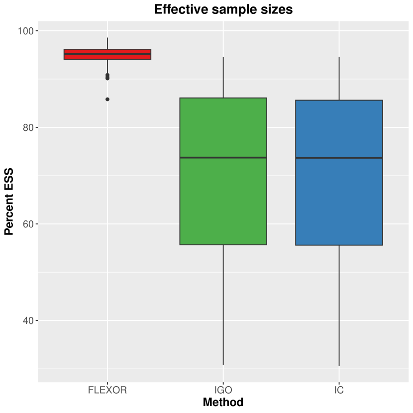
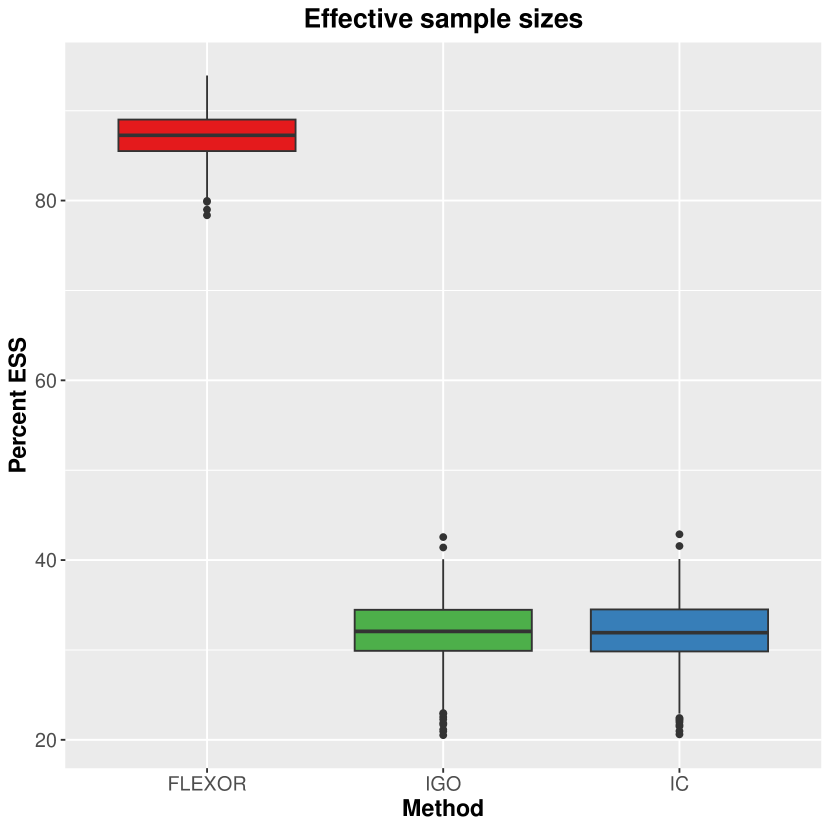
Figure 1: For the 500 simulated datasets, percentage ESS boxplots for the three pseudo-populations in the high (left panel) and low (right panel) simulation scenarios with $\tilde{N}=500$ subjects.

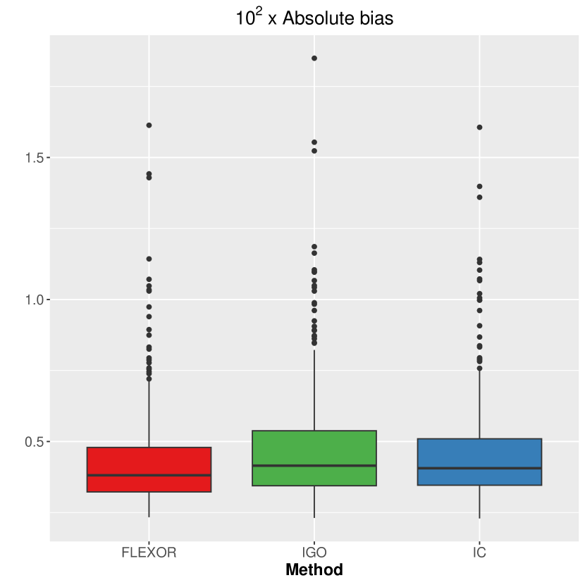
Figure 2: *

Absolute bias; High simulation scenario

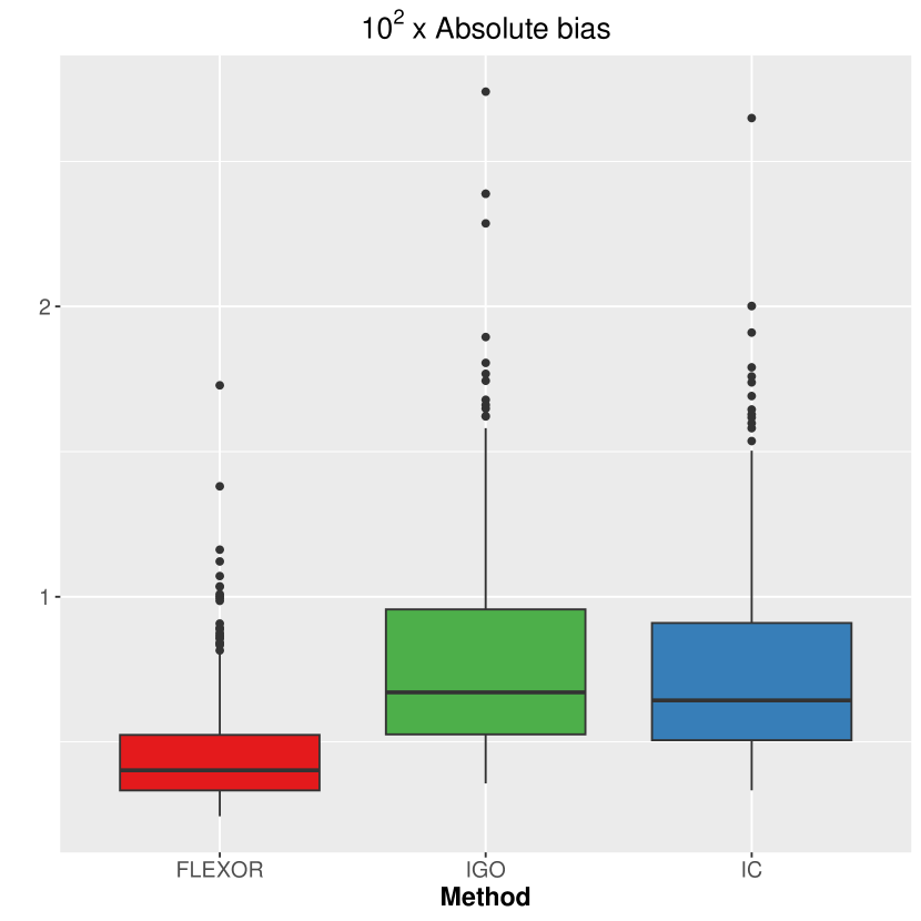
Figure 3: *

Absolute bias; Low simulation scenario

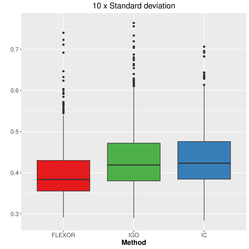
Figure 4: *

Standard deviation; High simulation scenario

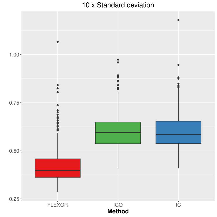
Figure 5: *

Standard deviation; Low simulation scenario

Figure 6: For the 500 simulated datasets, absolute biases (top panels) and standard deviations (bottom panels) for the group mean differences of the three pseudo-populations in the high (left panels) and low (right panels) simulation scenarios. For each artificial dataset and pseudo-population, the absolute bias and standard deviation were estimated using 500 bootstrap samples.

4 Meta-analysis of multiple (multi-site) breast cancer studies

For demonstrating the use of the WMAP package, we analyze a multi-site breast cancer study from The Cancer Genome Atlas (TCGA). The study was conducted across $J=7$ medical centers, including $N=450$ patients divided into $K=2$ groups based on breast cancer subtypes: infiltrating ductal carcinoma (IDC) and infiltrating lobular carcinoma (ILC); the dataset can be downloaded from the GDC Data Portal after registration (NCI, 2022). The dataset includes $p=30$ unbalanced covariates and the $L=8$ outcomes mimic the mRNA expression levels of targeted breast cancer genes, COL9A3, CXCL12, IGF1, ITGA11, IVL, LEF1, PRB2, and SMR3B (Christopoulos et al., 2015), in the TCGA datasets. We wish to estimate and compare the counterfactual means, standard deviations, and medians of the two groups representing disease subtypes IDC and ILC. The package facilitates the meta-analysis of the TCGA breast cancer, and other similar cancer datasets, which can help us better understand cancer oncogenesis.

4.1 Data structure

The package contains an R replication file named demoAnalyze.R to reproduce the results presented in this paper. We begin by installing and loading the WMAP package and the example dataset included in the package.

⬇

R> library(WMAP)

R> data(demo)

We then examine the contents of the dataset.

• X: $p=30$ demographic and clinicopathological covariates.

  ⬇

  R> dim(X)

  [1] 450 30

• Y: Outcome vectors of mRNA expression measurements for the eight targeted genes arranged in a $450\times 8$ matrix.

  ⬇

  R> round(head(Y),4)

  [,1] [,2] [,3] [,4] [,5] [,6] [,7] [,8]

  [1,] 1.2828 -0.1152 -0.3829 -0.3082 -1.1200 1.2068 -0.9472 0.8768

  [2,] -1.1603 1.5377 1.6034 -0.9822 -0.9507 0.3980 -0.9481 -0.2325

  [3,] -0.3815 1.1320 0.9348 -1.2661 1.1733 -0.0956 -0.1138 2.3797

  [4,] -0.3032 0.5999 1.3941 -0.0299 -1.1010 -0.0838 -0.9565 -0.5058

  [5,] 0.4147 -0.3312 -1.7675 0.7626 -1.1300 -0.6157 -0.4613 -0.9950

  [6,] 0.1867 0.9826 1.2274 0.7895 0.2217 -0.5541 -0.9479 -1.0016

• S: Site labels of patients, representing the seven medical centers.

• Z: Group labels of patients, representing the two disease subtypes IDC and ILC.

• groupnames:

  ⬇

  R> groupNames

  [1] "Infiltrating␣Ductal␣Carcinoma"

  [2] "Infiltrating␣Lobular␣Carcinoma"

• naturalGroupProp: The relative proportions of IDC and ILC subtypes in the larger U.S. population (Wright, 2022; Tran, 2022).

  ⬇

  R> naturalGroupProp

  [1] 0.8888889 0.1111111

Remark: Users can easily utilize the package functions to conduct meta-analyses on their own datasets. The formatting requirements for user-specified datasets are as follows: (a) Vector S, consisting of $N$ factor levels belonging to the set $\{1,\ldots,J\}$, representing the study memberships of the subjects. Each study must have at least 1 subject; (b) Vector Z, consisting of factor levels belonging to the set $\{1,\ldots,K\}$, representing the $N$ group memberships. Each group should contain at least 1 subject; (c) Covariate matrix, X, of dimension $N\times p$ containing $p$ continuous or binary (0/1) measurements, including factor covariates expanded as dummy binary values; (d) Matrix Y of dimension $N\times L$ comprising $L$ containing outcomes; and (e) Probabilty vector, naturalGroupProp, of length $K$ and strictly positive elements, representing the relative group prevalences $\boldsymbol{\theta}$ of the larger natural population. This last user input is necessary only for FLEXOR weights. It should be skipped for IC and IGO weights, which assume $\boldsymbol{\theta}=(1/K,\ldots,1/K)$; if specified, the input is ignored for these weighting methods.

4.2 Workflow of analysis

4.2.1 Stage 1: balancing.weights()

For a prespecified pseudo-population, function balancing.weights() first estimates the MPS and then calculates the subject-specific normalized balancing weights and sample ESS. The input arguments are summarized in Table I. The workflow, outlined in Algorithm 1, is based on the iterative Stage 1 procedure described in Section 2 and detailed in Algorithm 2. The function returns a list of items summarized in Table II. If method is “IC” or “IGO,” many arguments of balancing.weights() are not required and any user-provided values are ignored. For instance, $\gamma_{s}=1/J$ and $\theta_{z}=1/K$ are fixed for these pseudo-populations.

For the FLEXOR pseudo-population, (i) the function assumes that the $K$ group proportions $\boldsymbol{\theta}$ are fixed and specified by the user in vector naturalGroupProp, (ii) optional arguments, gammaMin and gammaMax, represent bounds for each element of the FLEXOR study proportions $\breve{\boldsymbol{\gamma}}$. In other words, $\Upsilon=\mathcal{S}_{J}\cap\bigl{(}[\text{\tt gammaMin},\text{\tt gammaMax}\bigr{)}]^{J}\times\{\boldsymbol{\theta}\}$ in the iterative steps to estimate the FLEXOR pseudo-popuation, and (iii) optional argument num.random indicates the number of random starting points for $(\boldsymbol{\gamma},\boldsymbol{\theta})\in\Upsilon$. The sample ESS maximized over these num.random independent replications identify the estimated FLEXOR pseudo-population, for which the $N$ sample weights and ESS comprise the function’s output.

Table I: Input arguments for function balancing.weights().

Argument	Short description	Default
S	Vector of factor levels representing the $N$ study	-
	memberships. Takes values in $\{1,\ldots,J\}$
Z	Vector of factor levels representing the $N$	-
	group memberships. Takes values in $\{1,\ldots,K\}$
X	Covariate matrix of $N$ rows and $p$ columns	-
method	Pseudo-population, i.e., weighting method;	-
	Can be "FLEXOR", "IC", or "IGO"
seed	Seed for random number generation	NULL
Relevant only when method="FLEXOR"; inputs ignored otherwise
naturalGroupProp	Relevant only for FLEXOR pseudo-populations:	-
	fixed user-specific probability vector $\boldsymbol{\theta}$
num.random	Number of random starting points of $\boldsymbol{\gamma}$	40
	in the iterative procedure
gammaMin	Lower bound for each $\gamma_{s}$ in the iterative procedure	0.001
gammaMax	Upper bound for each $\gamma_{s}$ in the iterative procedure	0.999

Table II: Output list components of function balancing.weights().

Position	Names	Short description
1	wt.v	$N$ empirically normalized sample weights
2	percentESS	Percentage sample ESS for pseudo-population

Input₁: S, Z, X, method, seed, naturalGroupProp, num.random, gammaMin, gammaMax

$\triangleright$ See Table I for input argument details

Function balancing.weights(Input₁):

   

   Regress (S,Z) on X and evaluate $\hat{\delta}_{s_{1}z_{1}}(\mathbf{x}_{1}),\ldots,\hat{\delta}_{s_{N}z_{N}}(\mathbf{x}_{N})$ $\triangleright$ Estimate MPS

   if method="IC" then

       for $i=1,\ldots,N$ do

          $\tilde{\rho}_{i}\leftarrow$ $1/\hat{\delta}_{s_{i}z_{i}}(\mathbf{x}_{i})$ $\triangleright$ IC unnormalized weights

       end for

      

    end if

   

   if method="IGO" then

       for $i=1,\ldots,N$ do

          $\eta(\mathbf{x}_{i})\leftarrow 1/\sum_{s=1}^{J}\sum_{z=1}^{K}\hat{\delta}_{sz}^{-1}(\mathbf{x}_{i})$ $\triangleright$ IGO tilting function

         $\tilde{\rho}_{i}\leftarrow$ $\eta(\mathbf{x}_{i})/\hat{\delta}_{s_{i}z_{i}}(\mathbf{x}_{i})$ $\triangleright$ IGO unnormalized weights

       end for

      

    end if

   

   if method="FLEXOR" then

       $\boldsymbol{\theta}\leftarrow$ naturalGroupProp $\triangleright$ fixed group prevalence

      for $t=1,\ldots,\text{\tt num.random}$ do

         

         $\boldsymbol{\gamma}^{(t)}\stackrel{{\scriptstyle i.i.d.}}{{\sim}}\mathcal{S}_{J}\cap\bigl{(}[\text{\tt gammaMin},\text{\tt gammaMax}\bigr{)}]^{J}$ $\triangleright$ random starting point

         $\boldsymbol{\gamma}^{(t)}_{{\dagger}},\mathcal{Q}^{(t)}\leftarrow$ FLEXOR.2STEP$\bigl{(}\cdots,\boldsymbol{\theta},\{\hat{\delta}_{s_{i}z_{i}}(\mathbf{x}_{i})\}_{i=1}^{N},\boldsymbol{\gamma}^{(t)}\bigr{)}$

          $\triangleright$ See Algorithm 2

       end for

      

      $\breve{t}\leftarrow\text{argmax}_{t}\mathcal{Q}^{(t)}$

      $\breve{\boldsymbol{\gamma}}\leftarrow\boldsymbol{\gamma}^{(\breve{t})}$

      $\mathcal{Q}\leftarrow$ OPTIMIZED.ESS$\bigl{(}\breve{\boldsymbol{\gamma}},\boldsymbol{\theta},\{\hat{\delta}_{s_{i}z_{i}}(\mathbf{x}_{i})\}_{i=1}^{N}\bigr{)}$ $\triangleright$ See Algorithm 2

      for $i=1,\ldots,n$ do

          $\eta(\mathbf{x}_{i})\leftarrow$ $\biggl{(}\sum_{s=1}^{J}\sum_{z=1}^{K}\frac{\breve{\gamma}_{s}^{2}\theta_{z}^{2}}{\delta_{sz}(\mathbf{x}_{i})}\biggr{)}^{-1}$

          $\triangleright$ Best fixed-$(\boldsymbol{\gamma},\boldsymbol{\theta})$ tilting function

       end for

      

      for $i=1,\ldots,N$ do

          $\tilde{\rho}_{i}\leftarrow$ $\breve{\gamma}_{s_{i}}\theta_{z_{i}}\eta(\mathbf{x}_{i})/\hat{\delta}_{s_{i}z_{i}}(\mathbf{x}_{i})$ $\triangleright$ FLEXOR unnormalized weights

       end for

      

      for $i=1,\ldots,N$ do

          $\rho_{i}=\tilde{\rho}_{i}/\sum_{u=1}^{N}\tilde{\rho}_{u}$ $\triangleright$ Empirically normalized weights

       end for

      

    end if

   

   return Empirically normalized weights, wt.v $\equiv\{\rho_{i}\}_{i=1}^{N}$ and percentESS $\equiv 100\mathcal{Q}/N$; see Table II for output details.

End Function

Algorithm 1 Stage 1 analysis: Empirically normalized balancing weights

Input: S, Z, X, gammaMin, gammaMax, $\boldsymbol{\theta},\{\hat{\delta}_{s_{i}z_{i}}(\mathbf{x}_{i})\}_{i=1}^{N}$, $\boldsymbol{\gamma}^{(t)}$ $\triangleright$ passed by Algorithm 1

Function FLEXOR.2STEP(Input):

   

   $\boldsymbol{\gamma}\leftarrow\boldsymbol{\gamma}^{(t)}$; $\mathcal{Q}^{(\text{new})}=0$; exit=FALSE $\triangleright$ Initialize

   $\boldsymbol{\Gamma}\leftarrow\mathcal{S}_{J}\cap\bigl{(}[\text{\tt gammaMin},\text{\tt gammaMax}\bigr{)}]^{J}$ $\triangleright$ Admissible values of $\boldsymbol{\gamma}$

   while !exit do

       $\mathcal{Q}^{(\text{old})}\leftarrow\mathcal{Q}^{(\text{new})}$

      $\boldsymbol{\gamma}^{{\dagger}}\leftarrow\text{argmax}_{\boldsymbol{\gamma}\in\boldsymbol{\Gamma}}$ OPTIMIZED.ESS$\bigl{(}\boldsymbol{\gamma},\boldsymbol{\theta},\{\hat{\delta}_{s_{i}z_{i}}(\mathbf{x}_{i})\}_{i=1}^{N}\bigr{)}$ $\triangleright$ function defined below

      $\mathcal{Q}^{(\text{new})}=$ OPTIMIZED.ESS$\bigl{(}\boldsymbol{\gamma}^{{\dagger}},\boldsymbol{\theta},\{\hat{\delta}_{s_{i}z_{i}}(\mathbf{x}_{i})\}_{i=1}^{N}\bigr{)}$

      if $\mathcal{Q}^{(\text{new})}/\mathcal{Q}^{(\text{old})}-1$ is small then

          exit $\leftarrow$ TRUE

       end if

      

    end while

   

   return $\boldsymbol{\gamma}^{{\dagger}},\mathcal{Q}^{(\text{new})}$

End Function

Function Optimized.ESS($\boldsymbol{\gamma},\boldsymbol{\theta},\{\hat{\delta}_{s_{i}z_{i}}(\mathbf{x}_{i})\}_{i=1}^{N}$):

    $\triangleright$ Maximum ESS for pseudo-population parameters $(\boldsymbol{\gamma},\boldsymbol{\theta})$

   for $i=1,\ldots,n$ do

       $\breve{\eta}_{\boldsymbol{\gamma},\boldsymbol{\theta}}(\mathbf{x}_{i})\leftarrow$ $\biggl{(}\sum_{s=1}^{J}\sum_{z=1}^{K}\frac{\gamma_{s}^{2}\theta_{z}^{2}}{\delta_{sz}(\mathbf{x}_{i})}\biggr{)}^{-1}$

       $\triangleright$ Best fixed-$(\boldsymbol{\gamma},\boldsymbol{\theta})$ tilting function

    end for

   

   return Sample.ESS$\bigl{(}\boldsymbol{\gamma},\boldsymbol{\theta},\breve{\eta},\{\hat{\delta}_{s_{i}z_{i}}(\mathbf{x}_{i})\}_{i=1}^{N}\bigr{)}$ $\triangleright$ function defined below

End Function

Function Sample.ESS($\boldsymbol{\gamma},\boldsymbol{\theta},\eta,\{\hat{\delta}_{s_{i}z_{i}}(\mathbf{x}_{i})\}_{i=1}^{N}$):

    for $i=1,\ldots,N$ do

       $\tilde{\rho}_{i}\leftarrow$ $\gamma_{s_{i}}\theta_{z_{i}}\eta(\mathbf{x}_{i})/\hat{\delta}_{s_{i}z_{i}}(\mathbf{x}_{i})$ $\triangleright$ unnormalized weights

    end for

   

   for $i=1,\ldots,N$ do

       $\rho_{i}=\tilde{\rho}_{i}/\sum_{u=1}^{N}\tilde{\rho}_{u}$ $\triangleright$ Empirically normalized weights

    end for

   

   $\tilde{\mathcal{Q}}(\boldsymbol{\gamma},\boldsymbol{\theta},\breve{\eta}_{\boldsymbol{\gamma},\boldsymbol{\theta}})\leftarrow N^{2}/\sum_{i=1}^{N}\rho_{i}^{2}$

   return $\tilde{\mathcal{Q}}(\boldsymbol{\gamma},\boldsymbol{\theta},\eta_{\boldsymbol{\gamma},\boldsymbol{\theta}})$

End Function

Algorithm 2 Iterative procedure of estimating FLEXOR pseudo-population

For example, to calculate the FLEXOR weights, we load the package and data, set a random seed to ensure reproducibility, and set the number of starting points for the iterative procedure before calling balancing.weights():

⬇

R> library(WMAP)

R> data(demo)

R> set.seed(1)

R> num.random=25

R> output1 = balancing.weights(S, Z, X, method="FLEXOR",

+ naturalGroupProp=naturalGroupProp, num.random)

[1] "FLEXOR...␣estimate␣10"

[1] "FLEXOR...␣estimate␣20" \end{lstlisting}

The output \texttt{output1} is a result S3 list object of class ‘\texttt{balancing\_weights}’, which contains:

\begin{itemize}

\item \texttt{wt.v}: the weights for each individual.

\begin{lstlisting}

R> length(output1$wt.v)

[1] 450

percentESS: the ESS of the FLEXOR weights.

⬇

R> output1$percentESS

[1] 34.62166

4.2.2 Stage 2: causal.estimate()

For a prespecified pseudo-population, the function causal.estimate() first calculates the subject-specific normalized balancing weights and sample ESS by a call to the balancing.weights() function. Next, it estimates the means, standard deviations and medians of the counterfactual outcomes of the group $K$, in addition to the mean differences in the group. Finally, the function regenerates the bootstrap samples and estimates the same set of counterfactual features for the bootstrap samples. The input arguments are summarized in Table III. The workflow is illustrated for counterfactual means and SD in Algorithm 3. The function returns a list of items summarized in Table IV.

Inputs₂: S, Z, X, Y, B, method, seed, naturalGroupProp, num.random, gammaMin, gammaMax

$\triangleright$ See Table III for input argument details

Function Causal.Estimate(Inputs₂):

   

   Inputs${}_{1}\leftarrow$ S, Z, X, method, seed, naturalGroupProp, num.random, gammaMin, gammaMax

   wt.v, percentESS $\leftarrow$ BALANCING.WEIGHTS(Inputs₁) $\triangleright$ see Algorithm 1

   $\rho_{1},\ldots,\rho_{n}\equiv$ wt.v $\triangleright$ empirically normalized weights

   for $z=1,\ldots,K$ do

       $\hat{\lambda}_{z}\leftarrow\frac{\sum_{i=1}^{N}\rho_{i}\,Y_{i}\,\mathcal{I}(Z_{i}=z)}{\sum_{i=1}^{N}\rho_{i}\,\mathcal{I}(Z_{i}=z)}$ $\triangleright$ estimated $z$th group’s counterfactual mean

      $\hat{\sigma}_{z}\leftarrow\biggl{(}\frac{\sum_{i=1}^{N}\rho_{i}\,Y_{i}^{2}\,\mathcal{I}(Z_{i}=z)}{\sum_{i=1}^{N}\rho_{i}\,\mathcal{I}(Z_{i}=z)}-\hat{\lambda}_{z}^{2}\biggr{)}^{1/2}$ $\triangleright$ estimated $z$th group’s counterfactual SD

    end for

   

   

   for $b=1,\ldots,B$ do

       Draw bootstrap sample S_b, Z_b, X_b, Y_b

      Inputs${}_{1b}\leftarrow$ S_b, Z_b, X_b, method, seed, naturalGroupProp, num.random, gammaMin, gammaMax

      wt_b.v, percentESS_b $\leftarrow$ BALANCING.WEIGHTS(Inputs_1b) $\triangleright$ see Algorithm 1

      $\rho_{1b},\ldots,\rho_{nb}\equiv$ wt_b.v $\triangleright$ empirically normalized weights

      for $z=1,\ldots,K$ do

          $\hat{\lambda}_{zb}\leftarrow\frac{\sum_{i=1}^{N}\rho_{ib}\,Y_{ib}\,\mathcal{I}(Z_{ib}=z)}{\sum_{i=1}^{N}\rho_{ib}\,\mathcal{I}(Z_{ib}=z)}$ $\triangleright$ estimated $z$th group’s counterfactual mean

         $\hat{\sigma}_{zb}\leftarrow\biggl{(}\frac{\sum_{i=1}^{N}\rho_{ib}\,Y_{ib}^{2}\,\mathcal{I}(Z_{ib}=z)}{\sum_{i=1}^{N}\rho_{ib}\,\mathcal{I}(Z_{ib}=z)}-\hat{\lambda}_{zb}^{2}\biggr{)}^{1/2}$ $\triangleright$ estimated $z$th group’s counterfactual SD

       end for

      

    end for

   

   return percentESS, estimates of means $\{\hat{\lambda}_{z}\}_{z=1}^{K}$, SDs $\{\hat{\sigma}_{z}\}_{z=1}^{K}$, bootstrap means $\{\hat{\lambda}_{zb}\}_{z=1}^{K}$, bootstrap SDs $\{\hat{\sigma}_{zb}\}_{z=1}^{K}$. See Table II for all outputs of the actual implementation.

End Function

Algorithm 3 Causal estimation of counterfactual means and SDs

Using the example dataset included with the WMAP package, we provide a step-by-step guide to the causal estimation of different features of the group-specific counterfactual outcomes for the three weighting methods, FLEXOR, integrative combined (IC), and integrative generalized overlap (IGO). As mentioned, the $K=2$ groups of the example dataset simulate the breast cancer subtypes, IDC and ILC, and the $L=8$ outcomes corresponding to the mRNA expression levels of the targeted breast cancer genes, COL9A3, CXCL12, IGF1, ITGA11, IVL, LEF1, PRB2, and SMR3B. The goal is unconfounded, covariate-balanced inference about the group counterfactual means, standard deviations, and medians, as well as counterfactual differences in group means and ratios of group standard deviations. If necessary, load the necessary packages and data, set a random seed, and set the runtime parameters:

⬇

R> library(WMAP)

R> data(demo)

R> set.seed(1)

R> num.random=25

R> B=200

Table III: Input arguments for function causal.estimate().

Argument	Short description	Default
S	Vector of factor levels representing the $N$ study	-
	memberships. Takes values in $\{1,\ldots,J\}$
Z	Vector of factor levels representing the $N$	-
	group memberships. Takes values in $\{1,\ldots,K\}$
X	Covariate matrix of $N$ rows and $p$ columns	-
Y	Matrix of $L$ outcomes, dimension $N\times L$	-
B	Number of bootstrap samples for variance estimation	100
method	Pseudo-population, i.e., weighting method;	-
	Can be "FLEXOR", "IC", or "IGO"
seed	Seed for random number generation	NULL
Relevant only when method="FLEXOR"; inputs ignored otherwise
naturalGroupProp	Relevant only for FLEXOR pseudo-populations:	-
	fixed user-specific probability vector $\boldsymbol{\theta}$
num.random	Number of random starting points of $\boldsymbol{\gamma}$	40
	in the iterative procedure
gammaMin	Lower bound for each $\gamma_{s}$ in the iterative procedure	0.001
gammaMax	Upper bound for each $\gamma_{s}$ in the iterative procedure	0.999

Then, call causal.estimate() setting method equal to "FLEXOR", "IGO", or "IC". For example, the following command applies the FLEXOR weighting method.

⬇

R> output2.f = causal.estimate(S, Z, X, Y, B, method="FLEXOR",

+ naturalGroupProp=naturalGroupProp, num.random)

Table IV: Output list components of function causal.estimate().

Position	Names	Short description
1	percentESS	Percentage sample ESS of pseudo-population
2	moments.ar	Array of dimension $3\times K\times L$, containing
		$\bullet$ estimated means, SDs, and medians (dimension 1)
		$\bullet$ for $K$ groups (dimension 2)
		$\bullet$ and $L$ counterfactual outcomes (dimension 3)
3	otherFeatures.v	Estimated mean group differences for $L$ outcomes
4	collatedMoments.ar	Array of dimension $3\times K\times L\times B$, containing
		$\bullet$ moments.ar of $b$th bootstrap sample (dimensions 1–3)
		$\bullet$ for $B$ bootstrap samples (dimension 4)
5	collatedOtherFeatures.mt	Matrix of dimension $L\times B$ containing
		$\bullet$ otherFeatures.v of $b$th bootstrap sample (dimension 1)
		$\bullet$ for $B$ bootstrap samples (dimension 2)
6	collatedESS	A vector of length $B$, containing
		$\bullet$ percentage sample ESS for $B$ bootstrap samples
7	method	Pseudo-population method, i.e., weighting method.

The output output2.f is a result S3 list object of class ‘causal_estimates’, which contains:

• percentESS: the ESS of the FLEXOR weights.

  ⬇

  R> output2.f$percentESS

  [1] 34.62166

• moments.ar: the means, standard deviations, and medians of the mRNA expression of the 8 genes in the $K=2$ groups.

  ⬇

  R> output2.f$moments.ar

  , , 1

  group 1 group 2

  mean -0.06417815 -0.08867675

  sd 0.92858998 0.60111155

  median -0.11474907 -0.05937943

  , , 2

  group 1 group 2

  mean 0.006908613 0.3910141

  sd 0.980184390 0.8207180

  median 0.092934721 0.4674662

  ...

  , , 8

  group 1 group 2

  mean -0.6221647 0.08445272

  sd 0.7286661 1.02987578

  median -0.8699967 -0.10213382

• otherFeatures.v: the mean differences of the 8 genes between the two groups.

  ⬇

  R> output2.f$otherFeatures.v

  [1] 0.0244986 -0.3841055 -0.6304299 0.2305657

  [5] 0.4334559 -0.2463727 -0.1624729 -0.7066175

• collatedMoments.ar: the moments.ar for each bootstrap.

• collatedOtherFeatures.mt: the mean differences of the 8 genes between the two groups (otherFeatures.v) for each bootstrap sample.

Based on the bootstrap results, we can calculate 95% confidence intervals, for example, for the mean differences of the eight genes:

⬇

R> CI.f = round(t(apply(output2.f$collatedOtherFeatures.mt, 1,

+ function(x) quantile(x,probs = c(0.025,0.975)))),2)

R> CI.f

2.5% 97.5%

[1,] -0.43 0.17

[2,] -1.07 -0.18

[3,] -1.15 -0.38

[4,] -0.44 0.35

[5,] 0.01 0.61

[6,] -0.67 0.00

[7,] -0.39 0.21

[8,] -1.12 -0.23

To calculate the 95% confidence intervals of the mean, median, and standard deviation for the mRNA expression levels of the eight genes in the two groups, we implement the following:

⬇

R> f.moments.ci = apply(output2.f$collatedMoments.ar, c(1, 2, 3), function(x) {

+ quantile(x, probs = c(0.025,0.975))

+ })

R> f.moments.ci

, , group 1, 1

mean sd median

2.5% -0.2772703 0.8530954 -0.32738785

97.5% 0.2135794 1.2989337 0.07514511

, , group 2, 1

mean sd median

2.5% -0.1110545 0.4694307 -0.2005817

97.5% 0.3571371 0.7961655 0.4898150

...

, , group 1, 8

mean sd median

2.5% -0.7442217 0.4668913 -0.9079259

97.5% -0.4562458 1.1208505 -0.7968190

, , group 2, 8

mean sd median

2.5% -0.3631548 0.7795273 -0.7489346

97.5% 0.4444478 1.2339100 0.5691793

To include the 95% CI in the output, we define a function write_res:

⬇

R> write_res = function(estimates, CI){

+ lower_bound <- CI[, 1] # 2.5% confidence bound

+ upper_bound <- CI[, 2] # 97.5% confidence bound

+

+ sapply(1:length(estimates), function(i) {

+ paste0(round(estimates[i],2), "␣(", round(lower_bound[i], 2), ",",

+ round(upper_bound[i], 2), ")")

+ })

+ }

and then use write_res to output results including point estimates and CIs separately for each comparison group:

⬇

R> f.moments = list()

R> for(i in 1:8){

+ f.moments[[i]] = cbind(group1 = write_res(output2.f$moments.ar[,1,i],

+ t(f.moments.ci[,,1,i])), # group 1 mean sd median

+ group2 = write_res(output2.f$moments.ar[,2,i],

+ t(f.moments.ci[,,2,i]))) # group 2 mean sd median

+

+ }

R> f.moments

[[1]]

group1 group2

[1,] "-0.06␣(-0.28,0.21)" "-0.09␣(-0.11,0.36)"

[2,] "0.93␣(0.85,1.3)" "0.6␣(0.47,0.8)"

[3,] "-0.11␣(-0.33,0.08)" "-0.06␣(-0.2,0.49)"

[[2]]

group1 group2

[1,] "0.01␣(-0.18,0.3)" "0.39␣(0.28,1.07)"

[2,] "0.98␣(0.8,1.13)" "0.82␣(0.57,1.13)"

[3,] "0.09␣(-0.19,0.34)" "0.47␣(0.2,1.27)"

...

[[8]]

group1 group2

[1,] "-0.62␣(-0.74,-0.46)" "0.08␣(-0.36,0.44)"

[2,] "0.73␣(0.47,1.12)" "1.03␣(0.78,1.23)"

[3,] "-0.87␣(-0.91,-0.8)" "-0.1␣(-0.75,0.57)"

For the other implemented weighting methods, i.e., IGO and IC, we would change the method argument in causal.estimate() to "IGO" and "IC", and follow the same procedures as above to obtain estimates and confidence intervals. More specifically, we apply the following commands:

⬇

R> output2.igo = causal.estimate(S, Z, X, Y, B, method="IGO")

R> output2.ic = causal.estimate(S, Z, X, Y, B, method="IC")

4.3 Discussion of results

Applying causal.estimate() to compute all the estimates along with their corresponding 95% confidence intervals, we summarize the results in Table LABEL:tab1. It appears that all three methods, i.e., FLEXOR, IC, and IGO, consistently indicated no significant difference in the counterfactual mean expression level of the COL9A3 gene between the invasive ductal carcinoma (IDC) and invasive lobular carcinoma (ILC) groups. However, a notable distinction in variability was observed, with IDC exhibiting significantly greater variability in expression levels compared to ILC. This elevated variability in IDC might reflect the inherently heterogeneous nature of this subtype, which is associated with a more diverse molecular landscape and potentially distinct tumor microenvironmental influences (Wang et al., 2024). Such variability could have implications for treatment responsiveness, as tumors with higher expression variability might exhibit differential sensitivity to targeted therapies. In contrast, the genes CXCL12 and IGF1 demonstrated significantly lower counterfactual mean expression levels in IDC compared to ILC. This observation aligns with the biological roles of these genes: CXCL12, a chemokine, is integral to cell migration and tumor metastasis, while IGF1 is known to play a role in cell growth, survival, and resistance to apoptosis. The reduced expression of these genes in IDC may indicate a subtype-specific divergence in signaling pathways that govern tumor progression. For instance, the lower CXCL12 expression in IDC may suggest altered stromal-tumor interactions, potentially impacting metastasis patterns. Similarly, the diminished IGF1 levels could reflect differences in the reliance on growth factor signaling between IDC and ILC, with implications for pathway-specific therapeutic targeting (Vanden Bempt et al., 2005). Interestingly, unlike COL9A3, the variability in expression levels for CXCL12 and IGF1 did not differ significantly between the subtypes. This uniformity in variability suggests that while these genes differ in their average expression levels, the regulatory mechanisms governing their expression stability may be conserved across IDC and ILC. This could indicate that the observed differences in mean expression are primarily driven by upstream genetic or epigenetic alterations rather than stochastic fluctuations (Samani et al., 2007). The unconfounded gene expression differences detected through this meta-causal analysis, encompassing both mean and variability distinctions between IDC and ILC, hold significant clinical implications. Specifically, the elevated variability in COL9A3 expression in IDC could serve as a biomarker for identifying high-risk patients who may benefit from intensified monitoring or tailored interventions. Meanwhile, the lower mean expression levels of CXCL12 and IGF1 in IDC suggest these genes could be leveraged as diagnostic markers to distinguish between subtypes or as therapeutic targets for subtype-specific treatment strategies. Furthermore, these findings may contribute to the development of novel prognostic models that integrate both mean expression levels and variability metrics to predict patient outcomes more accurately (McCart Reed et al., 2021). Finally, we note that in nearly all cases, the FLEXOR method outperformed the IC and IGO methods by producing notably tighter confidence intervals. This superior precision highlights the practical utility of FLEXOR in genomic research, where high-confidence estimates are critical for unraveling complex biological phenomena and informing translational applications. The enhanced resolution provided by FLEXOR could facilitate the identification of subtle yet clinically meaningful expression differences, further advancing personalized oncology.

Table V: For three targeted genes, COL9A3, CXCL12 and IGF1, the estimates and 95% bootstrap confidence levels (shown in parenthesis) of different population-level estimands of the potential outcomes of group 1 (IDC cancer subtype, denoted by superscript 1) and group 2 (ILC cancer subtype, denoted by superscript 2) with FLEXOR, IC, and IGO weights. An IC or IGO confidence interval is bolded if it is wider than the FLEXOR confidence interval. $\lambda$: group mean; $\sigma$: group standard deviation; $M$: group median.

COL9A3
Estimand	FLEXOR	IC	IGO
$\lambda^{(1)}$	$-0.06(-0.28,0.21)$	$0.02\boldsymbol{(-0.33,0.32)}$	$-0.04\boldsymbol{(-0.34,0.33)}$
$\lambda^{(2)}$	$-0.09(-0.11,0.36)$	$-0.04\boldsymbol{(-0.24,0.39)}$	$0.00\boldsymbol{(-0.33,0.46)}$
$\sigma^{(1)}$	$0.93(0.85,1.3)$	$1.09\boldsymbol{(0.8,1.32)}$	$1.04\boldsymbol{(0.8,1.34)}$
$\sigma^{(2)}$	$0.6(0.47,0.8)$	$0.67\boldsymbol{(0.43,0.83)}$	$0.68\boldsymbol{(0.42,0.87)}$
$M^{(1)}$	$-0.11(-0.33,0.08)$	$-0.12\boldsymbol{(-0.47,0.2)}$	$-0.12\boldsymbol{(-0.49,0.22)}$
$M^{(2)}$	$-0.06(-0.2,0.49)$	$-0.06\boldsymbol{(-0.37,0.53)}$	$0.06\boldsymbol{(-0.48,0.61)}$
$\lambda^{(1)}-\lambda^{(2)}$	$0.02(-0.43,0.17)$	$0.06\boldsymbol{(-0.65,0.28)}$	$-0.04\boldsymbol{(-0.63,0.39)}$
${\sigma^{(1)}}/{\sigma^{(2)}}$	$1.54(1.23,2.4)$	$1.62\boldsymbol{(1.14,2.62)}$	$1.54\boldsymbol{(1.12,2.85)}$
CXCL12
Estimand	FLEXOR	IC	IGO
$\lambda^{(1)}$	$0.01(-0.18,0.3)$	$-0.04\boldsymbol{(-0.19,0.33)}$	$-0.08\boldsymbol{(-0.26,0.39)}$
$\lambda^{(2)}$	$0.39(0.28,1.07)$	$0.44\boldsymbol{(0.27,1.12)}$	$0.48(0.28,1.06)$
$\sigma^{(1)}$	$0.98(0.8,1.13)$	$0.96\boldsymbol{(0.79,1.16)}$	$0.98\boldsymbol{(0.75,1.15)}$
$\sigma^{(2)}$	$0.82(0.57,1.13)$	$0.86\boldsymbol{(0.57,1.2)}$	$0.94\boldsymbol{(0.52,1.11)}$
$M^{(1)}$	$0.09(-0.19,0.34)$	$0.06\boldsymbol{(-0.29,0.46)}$	$-0.07\boldsymbol{(-0.32,0.57)}$
$M^{(2)}$	$0.47(0.2,1.27)$	$0.54\boldsymbol{(0.14,1.22)}$	$0.72\boldsymbol{(0.11,1.22)}$
$\lambda^{(1)}-\lambda^{(2)}$	$-0.38(-1.07,-0.18)$	$-0.48\boldsymbol{(-1.18,-0.11)}$	$-0.56\boldsymbol{(-1.12,-0.11)}$
${\sigma^{(1)}}/{\sigma^{(2)}}$	$1.19(0.81,1.72)$	$1.12(0.79,1.66)$	$1.04\boldsymbol{(0.77,1.88)}$
IGF1
Estimand	FLEXOR	IC	IGO
$\lambda^{(1)}$	$0.16(-0.15,0.32)$	$0.14\boldsymbol{(-0.18,0.37)}$	$0.15\boldsymbol{(-0.25,0.42)}$
$\lambda^{(2)}$	$0.79(0.57,1.17)$	$0.8\boldsymbol{(0.44,1.24)}$	$0.78\boldsymbol{(0.45,1.23)}$
$\sigma^{(1)}$	$0.93(0.82,1.1)$	$1.01\boldsymbol{(0.77,1.15)}$	$1\boldsymbol{(0.78,1.18)}$
$\sigma^{(2)}$	$0.74(0.49,1.03)$	$0.8\boldsymbol{(0.48,1.09)}$	$0.86\boldsymbol{(0.43,1.14)}$
$M^{(1)}$	$0.26(-0.14,0.44)$	$0.35\boldsymbol{(-0.19,0.58)}$	$0.35\boldsymbol{(-0.22,0.64)}$
$M^{(2)}$	$0.91(0.78,1.25)$	$0.96\boldsymbol{(0.71,1.36)}$	$0.96\boldsymbol{(0.61,1.33)}$
$\lambda^{(1)}-\lambda^{(2)}$	$-0.63(-1.15,-0.38)$	$-0.66\boldsymbol{(-1.29,-0.24)}$	$-0.63\boldsymbol{(-1.27,-0.31)}$
${\sigma^{(1)}}/{\sigma^{(2)}}$	$1.26(0.89,1.92)$	$1.27\boldsymbol{(0.89,2.06)}$	$1.16\boldsymbol{(0.78,2.37)}$

5 Conclusions and Future Developments

Integrating multiple observational studies to make unconfounded causal or descriptive comparisons of group potential outcomes in large natural populations presents significant challenges, because of the complexities involved in data heterogeneity, selection bias, and the need for accurate balancing across datasets. Recently, Guha and Li (2024) introduced a unified weighting framework designed to address these challenges by extending inverse probability weighting techniques for integrative analyses. To translate this theoretical framework into practice, we have developed the R package WMAP. This software tool is specifically designed for the integrative analysis of user-specified datasets and implements three advanced weighting approaches, i.e., IC (Integrative Calibration), IGO (Integrative Generalized Optimization), and FLEXOR (Flexible Optimization of Weights). These methods enhance the capacity to estimate multiple propensity scores, compute balancing weights for subjects, evaluate effective sample sizes, and derive various estimands of counterfactual group outcomes. The package also includes functionality for calculating bootstrap variability estimates, which are essential for quantifying the uncertainty of the results. In a practical application, we have used WMAP to analyze differences in mean and standard deviation of gene expression levels between two major breast cancer subtypes, invasive ductal carcinoma (IDC) and invasive lobular carcinoma (ILC). This analysis yielded biologically meaningful results, highlighting the package’s potential for contributing to the understanding of complex biological systems. WMAP’s utility is not limited to observational studies. It is equally applicable to multi-arm randomized controlled trials (RCTs), particularly in scenarios where within-study allocation mechanisms are known. Furthermore, future updates to WMAP will extend its capabilities to support hybrid study designs that combine data from RCTs and retrospective cohorts. Current limitations, such as challenges in handling high-dimensional biomarker data, are actively being addressed in ongoing development. These enhancements will make WMAP an even more powerful tool for advancing integrative causal inference and descriptive analyses across a wide range of scientific and clinical research domains.

References

- Christopoulos et al. (2015) P. F. Christopoulos, P. Msaouel, and M. Koutsilieris. The role of the insulin-like growth factor-1 system in breast cancer. Molecular Cancer, 14(1):1–14, 2015.
- Crump et al. (2006) R. K. Crump, V. J. Hotz, G. W. Imbens, and O. A. Mitnik. Moving the goalposts: addressing limited overlap in the estimation of average treatment effects by changing the estimand. Technical report, National Bureau of Economic Research, 2006.
- Guha and Li (2024) S. Guha and Y. Li. Causal meta-analysis by integrating multiple observational studies with multivariate outcomes. Biometrics, 80(3):ujae070, 2024.
- Guha et al. (2024) S. Guha, M. Xu, K. Priyam, and Y. Li. WMAP: Weighted Meta-Analysis with Pseudo-Populations, 2024. URL https://CRAN.R-project.org/package=WMAP. R package version 1.0.0.
- Imbens (2000) G. W. Imbens. The role of the propensity score in estimating dose-response functions. Biometrika, 87(3):706–710, 2000.
- Li and Li (2019) F. Li and F. Li. Propensity score weighting for causal inference with multiple treatments. The Annals of Applied Statistics, 13(4):2389–2415, 2019.
- Li et al. (2018) F. Li, K. L. Morgan, and A. M. Zaslavsky. Balancing covariates via propensity score weighting. Journal of the American Statistical Association, 113(521):390–400, 2018.
- Li and Greene (2013) L. Li and T. Greene. A weighting analogue to pair matching in propensity score analysis. The International Journal of Biostatistics, 9(2):215–234, 2013.
- Lunceford and Davidian (2004) J. K. Lunceford and M. Davidian. Stratification and weighting via the propensity score in estimation of causal treatment effects: a comparative study. Statistics in Medicine, 23(19):2937–2960, 2004.
- McCaffrey et al. (2013) D. F. McCaffrey, B. A. Griffin, D. Almirall, M. E. Slaughter, R. Ramchand, and L. F. Burgette. A tutorial on propensity score estimation for multiple treatments using generalized boosted models. Statistics in Medicine, 32(19):3388–3414, 2013.
- McCart Reed et al. (2021) A. E. McCart Reed, S. Foong, J. R. Kutasovic, K. Nones, N. Waddell, S. R. Lakhani, and P. T. Simpson. The genomic landscape of lobular breast cancer. Cancers, 13(8):1950, 2021.
- NCI (2022) NCI. Genomic data commons data portal, 2022. https://portal.gdc.cancer.gov/.
- Robins and Rotnitzky (1995) J. M. Robins and A. Rotnitzky. Semiparametric efficiency in multivariate regression models with missing data. Journal of the American Statistical Association, 90(429):122–129, 1995.
- Rosenbaum and Rubin (1983) P. R. Rosenbaum and D. B. Rubin. The central role of the propensity score in observational studies for causal effects. Biometrika, 70(1):41–55, 1983.
- Rubin (2007) D. B. Rubin. The design versus the analysis of observational studies for causal effects: parallels with the design of randomized trials. Statistics in Medicine, 26:20–36, 2007.
- Samani et al. (2007) A. A. Samani, S. Yakar, D. LeRoith, and P. Brodt. The role of the igf system in cancer growth and progression: overview and recent insights. Endocrine Reviews, 28(1):20–47, 2007. doi:10.1210/er.2006-0001.
- Tran (2022) H.-T. Tran. Invasive lobular carcinoma, 2022. https://www.hopkinsmedicine.org/health/conditions-and-diseases/breast-cancer/invasive-lobular-carcinoma.
- Vanden Bempt et al. (2005) I. Vanden Bempt, V. Vanhentenrijk, M. Drijkoningen, and C. De Wolf-Peeters. Comparative expressed sequence hybridisation revealed distinct chromosomal regions of differential gene expression in breast cancer subtypes. Breast Cancer Research, 7:1–2, 2005.
- Wang et al. (2024) J. Wang, B. Li, M. Luo, J. Huang, K. Zhang, S. Zheng, S. Zhang, and J. Zhou. Progression from ductal carcinoma in situ to invasive breast cancer: molecular features and clinical significance. Signal Transduction and Targeted Therapy, 9(1):83, 2024.
- Wright (2022) P. Wright. Invasive ductal carcinoma, 2022. https://www.hopkinsmedicine.org/health/conditions-and-diseases/breast-cancer/invasive-ductal-carcinoma-idc.