Towards Adversarially Robust Deep Metric Learning

Abstract

Deep Metric Learning has shown remarkable successes in many domains by enjoying the powerful deep learning model. But deep learning models usually have vulnerabilities and could be easily fooled by adversarial examples. There are various defenses aiming at improving the adversarial robustness of the deep learning model, especially in classification tasks. However, there are few works that study the robustness of deep neural networks in deep metric learning tasks. In this work, we find that vulnerabilities still exist in deep metric learning tasks, and some SOTA defenses which work well in classification tasks fail in deep metric learning tasks. To reduce that threat of adversarial examples in deep metric learning tasks, we propose the Ensemble Adversarial Training (EAT) to alleviate the hazards caused by adversarial examples through promoting the diversity of the ensemble and introducing the self-transferring mechanism. Furthermore, we implement and evaluate our method on three widely-used datasets (CUB200, CARS196, and In-Shop). The results of experiments show that the proposed EAT method outperforms other defenses designed for classification tasks.

Introduction

Deep Learning has been widely used in computer vision (russakovsky2015imagenet), natural language processing (graves2014towards), and so on. Deep Metric Learning (DML) also has shown powerful capability on many domains such as face verification (schroff2015facenet), pedestrian re-identification (xiao2017joint), representation learning (qiao2019transductive), few-shot learning (kim2019deep), etc.

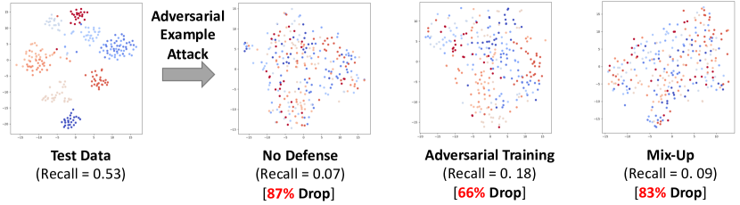
Figure 1: The t-SNE (Poliar731877) result of current popular defenses (Adversarial Training (madryDeepLearningModels2019a) and Mix-Up (zhangMixupEmpiricalRisk2018)) in the DML tasks on the CUB200 with the Proxy Anchor Loss (kimProxyAnchorLoss2020) under the adversarial example attacks. The result presents that current defenses fail in defending the adversarial examples in DML.

However, there is a thorn in Deep Learning – Adversarial Examples. Szegedy et al. (szegedyIntriguingPropertiesNeural2014) have shown the vulnerability of the deep neural networks. They found that an imperceptible perturbation on a natural image could greatly affect the result of the deep learning model. These perturbed images for fooling the model are called adversarial examples.

As for defending these adversarial examples, some recent works (maoMetricLearningAdversarial; DBLP:journals/corr/abs-1803-06373) exploit the training paradigm of metric learning to enhance the adversarial robustness in traditional classification tasks. However, few works discuss the adversarial robustness in DML tasks.

Facing adversarial examples on DML tasks, we find that DML is still vulnerable (even for the SOTA metric learning methods and defenses) as shown in Figure 1. There are two key challenges: (i) The instability of the target embedding; (ii) The inconsistency of the data manifold between the training and test dataset. Current popular defending strategies based on the Mix-Up methods (e.g. Mix-Up Training (zhangMixupEmpiricalRisk2018), Interpolated Adversarial Training (lambInterpolatedAdversarialTraining2019), etc.) rely on the fixed one-hot target vector. In DML tasks, the target representative embedding is changing during the training phase. Thus, these methods cannot work well due to that dynamic during the training phase in DML. In DML tasks, we usually divide the dataset by classes (i.e. A half of all classes is used for training) instead of dividing by the data (i.e. the model has known every class). There is an inconsistency of the data manifold distribution between the training and test dataset. The manifold distribution of adversarial examples is also different between these two datasets so it is harder to defend than traditional classification tasks.

In this paper, we propose a novel algorithm to enhance the adversarial robustness of DML called Ensemble Adversarial Training (EAT). We strengthen the robustness by promoting the diversity among these models in the ensemble and introducing the self-transferring mechanism. We exploit the division of the training data to construct various models instead of explicitly constraining the output in traditional classification tasks like (pangImprovingAdversarialRobustness2019).

We evaluate our algorithm on three popular datasets (CUB200 (WelinderEtal2010), CARS196 (KrauseStarkDengFei-Fei_3DRR2013), and In-Shop (liuLQWTcvpr16DeepFashion)) with two popular models (MobileNet-V2 (DBLP:journals/corr/abs-1801-04381) and BN-Inception (DBLP:journals/corr/IoffeS15)). Based on the SOTA metric learning loss (Proxy Anchor Loss, PAL (kimProxyAnchorLoss2020)), the proposed method outperforms other defenses which have been used in classification tasks. We also study the corresponding hyperparameters (the number of models and the coefficient of adversarial loss) of our methods.

The contributions of this paper are summarized below:

• We discover the vulnerability of DML in their metric tasks under adversarial examples (even for the SOTA DML method). We also reveal that it is no longer suitable to apply current popular defenses (e.g. Mix-Up Training, IAT, etc.) on DML.

• To the best of our knowledge, we are the first to propose a defense in DML against the adversarial examples. We propose the Ensemble Adversarial Training to enhance the adversarial robustness in DML by promoting the diversity of the ensemble and introducing the self-transferring mechanism.

• We implement our algorithm and evaluate the proposed method on three popular datasets (CUB200, CARS196, and In-Shop) with two models (MobileNetV2 and BN-Inception). Our results show the proposed method has SOTA performance in comparison with other popular defenses of classification tasks. Also, we further make the ablation study to analyze the robustness gain of our split mechanism and the whole EAT defense.

The rest of this paper is organized as follows. We first introduce some related works. Then, we formalize our problem and give some necessary definitions. Furthermore, we describe the proposed algorithm and some related details. Finally, we discuss our evaluation results in Experiments Section.

Related Works

Deep Metric Learning

DML aims to learn a distance representation for each input through deep neural networks (parkhi2015deep; schroff2015facenet). Similar inputs produce close representations in metric learning. The key to DML is the loss function. In the training step, the metric learning loss is computed by the tuple which consists of samples (similar samples and dissimilar samples) like the contrastive loss (bromley1994signature; chopra2005learning; hadsell2006dimensionality) and the triplet loss (schroff2015facenet).

The contrastive loss and the triplet loss are called pair-based loss and that kind of loss need to sample data and build the tuple for training. The sampling operation in pair-based loss causes high complexity. To reduce the complexity of the pair-based loss, the proxy-based methods (aziere2019ensemble) are introduced. The proxy-based methods always maintain proxies to represent each class and the corresponding loss is computed by the proxy with real samples. Furthermore, kimProxyAnchorLoss2020 (kimProxyAnchorLoss2020) proposed a novel proxy-based loss by making a combination of the SoftTriple Loss (qianSoftTripleLossDeep2020) and the Proxy-NCA Loss (movshovitz2017no).

Adversarial Example Attacks

Initially, szegedyIntriguingPropertiesNeural2014 (szegedyIntriguingPropertiesNeural2014) found that the deep neural network has vulnerability under some specific perturbations on the input. goodfellowExplainingHarnessingAdversarial2015 (goodfellowExplainingHarnessingAdversarial2015) proposed Fast Gradient Sign Method (FGSM). FGSM exploits the sign of gradients after the backpropagation to construct the perturbation. papernotLimitationsDeepLearning2015 (papernotLimitationsDeepLearning2015) proposed the Jacobian-based Saliency Map Attack (JSMA) by constructing a saliency map to guide the generation of adversarial examples. Carlini and Wagner (carliniEvaluatingRobustnessNeural2017) proposed the C&W attack which alleviates the linear property in the optimization which is used for searching the perturbation. madryDeepLearningModels2019a (madryDeepLearningModels2019a) proposed Projected Gradient Method (PGD) to further improve the attack performance by the project operation.

In this work, we follow (pangMixupInferenceBetter2020) and select the PGD attack to evaluate the robustness of the deep learning model because Recent works always follow the scheme of the PGD attack and make some variants.

Adversarial Example Defenses

The Adversarial Example Defenses focus on improving the adversarial robustness of the deep learning model. Those different defenses always add some additional operation on different steps (training step (goodfellowExplainingHarnessingAdversarial2015; zhangMixupEmpiricalRisk2018; vermaManifoldMixupBetter2019; madryDeepLearningModels2019a), inference step(xie2017mitigating; pangMixupInferenceBetter2020), etc.).

In the inference step, tabacof2016exploring (tabacof2016exploring) proposed a defense by performing some linear transformations (Gaussian Noise) on the input data to mitigating the effect of adversarial examples. guo2017countering (guo2017countering), xie2017mitigating (xie2017mitigating) and raff2019barrage (raff2019barrage) proposed the variant based on performing a non-linear transformation on the input of the deep learning model. pangMixupInferenceBetter2020 (pangMixupInferenceBetter2020) further proposed a novel defense based on the Mix-Up training paradigm. They directly perform the linear combination on inputs to alleviate the effect of the adversarial examples. Yet, these works do not consider the DML task and study the performance of the defense after transferring from the classification task.

In the training step, madryDeepLearningModels2019a (madryDeepLearningModels2019a) proposed a defense called Adversarial Training (AT) which exploits the strongest adversarial example attacks to generate adversarial examples for training a more robust deep learning model. AT methods have presented a more powerful effect on defending the adversarial examples than other defenses. lambInterpolatedAdversarialTraining2019 (lambInterpolatedAdversarialTraining2019) further proposed a defense called Interpolated Adversarial Training (IAT) which combines the Mix-Up methods with AT methods.

In addition, baiAdversarialMetricAttack2020 (baiAdversarialMetricAttack2020) proposed a defense for adversarial examples in Person Re-Identification task which utilizes the DML mechanism. However, they do not analyze the DML tasks and their threat model is only designed for the Person Re-Identification tasks.

Problem Formulation

Notations

We denote the DML model as $\mathcal{F}(x;\theta)$, which takes $m$-dimensional data $x\in\mathbb{R}^{m}$ as input and $\theta$ as model parameters. The output embedding of $\mathcal{F}(\cdot)$ is a vector with $d$ dimensions ($\mathcal{F}(x;\theta)=\hat{y}\in\mathbb{R}^{d}$). We denote the training dataset and the test dataset as $D_{train}=\{(x_{1},y_{1}),(x_{2},y_{2}),...,(x_{N},y_{N})\}$ and $D_{test}=\{(x_{1},y_{1}),(x_{2},y_{2}),...,(x_{M},y_{M})\}$, respectively. $N$ is the number of training samples and $M$ is the number of test samples. We represent the adversarial example of a specific input $x$ as $x_{adv}=x+\delta$, where $\delta$ is the perturbation computed by the attacker and usually has small amplitude. Following the same choice in (pangMixupInferenceBetter2020; zhangMixupEmpiricalRisk2018; madryDeepLearningModels2019a; vermaManifoldMixupBetter2019), in this paper, we use $l_{p}$-norm to bound $\delta$ and consider the $\delta$ s.t. $||\delta||_{p}\leq\varepsilon$ as valid perturbations.

Problem Definition

Before introducing the formal definition of the problem, we first review defending adversarial examples for traditional classification tasks, which can be written as:

$$\min_{\theta}\mathbb{E}_{(x,y)\sim D}\Big{[}\max_{x_{adv}\in S(x,\varepsilon)}\mathcal{L}(\mathcal{C}(x_{adv};\theta),y)\Big{]}$$ (1)

$S(x,\varepsilon)$ is the set of possible adversarial examples that satisfy $||x_{adv}-x||_{p}=||\delta||_{p}\leq\varepsilon$. And $\mathcal{L}(\cdot)$ is the loss function (e.g. cross-entropy loss) that evaluates the distance between the one-hot label ($y$) of $x$ and the output of classification model $\mathcal{C}(\cdot)$ when its input is $x_{adv}$. Given an input $x$, Equation 1 encourages $\mathcal{C}(\cdot)$ to produce similar outputs for all $x_{adv}\in S(x,\varepsilon)$, and thus making sure that the attacker cannot find the small perturbation $\delta$ that can fool the classifier.

However, Equation 1 cannot be used for DML because there is no explicit label ($y$) for the data samples in DML tasks. DML is designed to model the distance over data samples. In real world use, DML extracts embedding vectors from input data, and then treats data samples whose embedding vectors have small distances as the same class, while considers data samples whose embedding vectors have large distances as different classes. The label vector of a data sample is usually the centroid of the class it belongs to in the embedding space and is unclear untill the training of DML model is finished.

The loss function of DML always depends on several samples instead of one sample, and its general form can be well represented by the triplet loss (schroff2015facenet):

$$\mathcal{L}_{metric}(\mathcal{F}(x),\mathcal{F}(x^{+}),\mathcal{F}(x^{-}))=$$ (2)

$$||\mathcal{F}(x)-\mathcal{F}(x^{+})||+\max(0,m-||\mathcal{F}(x)-\mathcal{F}(x^{-})||)$$

where $x$, $x^{+}$ are data samples of the same class while $x^{-}$ is from another class, and $m$ is a constant number. Similarly to Equation 1, we can write the problem of defending adversarial examples for DML as:

$$\min_{\theta}\mathbb{E}_{(x,x^{+},x^{-})\sim D}\Big{[}\max_{x_{adv},x^{+}_{adv},x^{-}_{adv}\in S(x,x^{+},x^{-},\varepsilon)}$$ (3)

$$\mathcal{L}_{metric}(\mathcal{F}(x_{adv};\theta),\mathcal{F}(x^{+}_{adv};\theta),\mathcal{F}(x^{-}_{adv};\theta))\Big{]}$$

where $S(x,x^{+},x^{-},\varepsilon)$ is the abbreviation of $\{S(x,\varepsilon),S(x^{+},\varepsilon),S(x^{-},\varepsilon)\}$.

Previous Defenses

In this section, we will introduce four kinds of representative defense methods for classification models and analyse whether or not their design principles can be used in DML. We also give adapted forms of these defenses under DML.

Adversarial Training (AT). AT improves the adversarial robustness by introducing adversarial examples into the training phase. At each training iteration, AT generates adversarial examples based on the current model and include the adversarial examples into the training dataset. AT minimizes the empirical risk as:

$$\min_{\theta}\frac{1}{|D|}\sum_{(x,y)\in D}\mathcal{L}(\mathcal{C}(x_{adv}),y)$$ (4)

where $x_{adv}$ is generated by launching adversarial attacks. Taking the most powerful and representative attack – PGD (madryDeepLearningModels2019a) as an example, generating adversarial examples can be described as:

$$x_{adv}^{(t+1)}=\text{Proj}_{x+\mathcal{S}}\left(x_{adv}^{(t)}+\alpha\text{sgn}(\nabla_{x}\mathcal{L}(\mathcal{C}(x_{adv}^{(t)}),y))\right)$$ (5)

where $\text{Proj}_{x+\mathcal{S}}(z)$ is the projection function which can project the $z$ into the space $x+\mathcal{S}$ and $\mathcal{S}$ is the possible adversarial example space of the $x$.

For DML, since we do not have the label vector $y$ for each input sample $x$, to make AT available for DML, we can replace the $\mathcal{L}(\cdot)$, $\mathcal{C}(\cdot)$, and $y$ in Equation 4 and 5 with $\mathcal{L}_{metric}(\cdot)$, $\mathcal{F}(\cdot)$, and $\mathcal{F}(x)$, respectively. It is worth noting that the dynamic “label” $\mathcal{F}(x)$ could make the training hard to converge.

Mix-Up Training. Mix-Up Training methods have presented a great performance in improving the adversarial robustness of the deep neural network. These kinds of methods have lower complexity than the AT methods. The target of the Mix-Up Training methods can be written as:

$$\min_{\theta}\frac{1}{m}\sum_{i=1}^{m}{\mathcal{L}(\mathcal{C}(\tilde{x}_{i}),\tilde{y}_{i})}$$ (6)

where $\tilde{x}_{i}=\lambda x_{i0}+(1-\lambda)x_{i1}$, $\tilde{y}_{i}=\lambda y_{i0}+(1-\lambda)y_{i1}$, $\lambda\sim Beta(\alpha,\alpha)$ and $m$ is the number of training samples. Mix-Up Training methods exploit the linear combination of training sample instead of performing the adversarial attack for obtaining lower computation complexity. In fact, the key of those defenses is the data augmentation brought by the linear combination. For DML, we can replace the $\tilde{y}_{i}$ in Equation 6 as $\lambda\mathcal{F}(x_{i0})+(1-\lambda)\mathcal{F}(x_{i1})$, and replace the $\mathcal{L}(\cdot)$ and $\mathcal{C}(\cdot)$ with $\mathcal{L}_{metric}(\cdot)$ and $\mathcal{F}(\cdot)$, respectively.

Interpolated Adversarial Training (IAT) (lambInterpolatedAdversarialTraining2019). IAT is a fusion of the Mix-Up Training and AT. The target of IAT can be written as:

$$\min_{\theta}\frac{1}{m}\sum_{i=1}^{m}{\mathcal{L}(\mathcal{C}(\tilde{x}_{i}),\tilde{y}_{i})}+\frac{1}{m}\sum_{i=1}^{m}{\mathcal{L}(\mathcal{C}(g(\tilde{x}_{i})),\tilde{y}_{i})}$$ (7)

where $g(\tilde{x}_{i})=\lambda Adv(x_{i0})+(1-\lambda)Adv(x_{i1})$, $Adv(\cdot)$ is an arbitrary adversarial example attack and $\lambda\sim Beta(\alpha,\alpha)$. We can adapt IAT to DML by using the same method used for Mix-Up training.

However, the defenses based on the Mix-Up Training methods cannot work well for DML because these methods depend on stable label vectors ($y$). In DML, there is no such label vector, and the adapted $\tilde{y}_{i}=\lambda\mathcal{F}(x_{i0})+(1-\lambda)\mathcal{F}(x_{i1})$ is dynamic and changes as the update of $\mathcal{F}(\cdot)$, which may result in the effect that the training hard is hard to converge .

TRADES (zhangTheoreticallyPrincipledTradeoff2019). TRADES is a novel defense method which focus on the trade-off between robustness and accuracy. The target of TRADES can be written as:

$$\min_{\theta}\frac{1}{m}\sum_{i=0}^{m}\big{(}\mathcal{L}(C(x_{i}),y_{i})+\lambda\cdot\mathcal{L}(C(Adv(x_{i})),C(x_{i}))\big{)}$$ (8)

where $Adv(\cdot)$ is an arbitary adversarial example attack and $\lambda>0$ is the regularization parameter. TRADES presents great performance on classification tasks but it still relies on the one-hot target vector. In DML, we naturally change the first loss term to the metric loss and replace the $C(\cdot)$ with $\mathcal{F}(\cdot)$.

Ensemble Training. Pang et al. (pangImprovingAdversarialRobustness2019) proposed a defense by promoting the diversity of the ensemble to improve the adversarial robustness. They define the ensemble diversity as $\mathbb{ED}=\text{det}(M^{T}M)$ where $M=(\mathcal{F}^{(1)}(x),\mathcal{F}^{(2)}(x),...,\mathcal{F}^{(K)}(x))\in\mathbb{R}^{(L-1)\times K}$ and $\mathcal{F}^{(i)}$ is the order-preserving prediction of the $i$-th classifier on the input $x$. That defense is aiming to maximize the diversity term $\mathbb{ED}$ to 1. However, the explicit constraint of $\mathbb{ED}$ fail in DML because their diversity loss is hard to converge under the high dimensional embedding space of DML. Inspired by their work, we propose the Ensemble Adversarial Training for robust DML which is shown in Section Our Approach. We promote the diversity by the data division instead of using the determinant constraint. Furthermore, we introduce the self-transferring mechanism to improve the adversarial robustness of the whole ensemble.

Our Approach

Ensemble Adversarial Training

As discussed in Section Previous Defenses, defensive methods designed for classification models cannot be directly used for DML and their adapted forms also cannot work well because DML does not have explicit label vectors for data samples and the embeddings vectors are usually of high dimensions.

To handle those issues, we propose the Ensemble Adversarial Training method by promoting the diversity of the ensemble to improve the adversarial robustness. Additionally, we construct the self-transferring mechanism during the training step to further enhance the adversarial robustness of the ensemble.

As is shown in the algorithm 1, we first randomly split the training data into $N$ parts and every $N-1$ parts are the specific training set for each model of the ensemble (i.e. we train $i$-th model without the $i$-th part of all the parts of training data). Previous similar methods in traditional classification are trying to promote the diversity of the ensemble by adding an explicit constraint of the output vectors (e.g. the determinant $\text{det}(M^{T}M)$ where $M$ consists of all the output vector of the ensemble). Those methods are trying to make the output vectors of the deep neural networks orthogonal. But it is difficult to learn such a deep learning model in the metric learning tasks due to the high dimensional space of the output embedding and the numerical instability of the target vector.

After the distribution of the training data for different models of the ensemble, we apply the metric learning loss (e.g. PAL) on each data for each model. Then, we perform the PGD attack on all the models with $N-1$ parts of training data for each model and obtain the adversarial loss for each model. The computing process of the adversarial loss is called the self-transferring mechanism (i.e. Transferring the robustness from the other models). Our final target loss is the linear combination of the adversarial loss and the metric learning loss. Based on that final loss, we perform the variant of the Stochastic Gradient Descent (Weighted Adam) to optimize the parameters of each model.

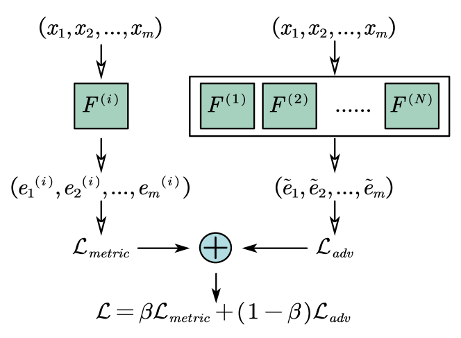
Figure 2: Ensemble Adversarial Training for $i$-th Model of the Ensemble. We generate the adversarial example for training by using the whole ensemble. That is our self-transferring mechanism which can transfer the robustness from other models in the ensemble.

Algorithm 1 Ensemble Adversarial Training

0: $N$ individual models: $\mathcal{F}^{i}_{\theta^{i}}$ where $1\leq i\leq N$, Training Data: $D_{train}=\{(x_{i},y_{i})\}_{i=1}^{|D_{train}|}$, Epochs: $T$, perturbation budget: $\varepsilon$, learning rate: $\gamma$, mixed ratio: $\beta$

0: Updated parameters: $\theta^{i}_{T}$

1: Initialize the parameters $\theta^{i}=\theta^{i}_{0}$

2: Splitting the training dataset into $N$ parts $D_{train}=\{D_{train}^{1},D_{train}^{2},...,D_{train}^{N}\}$ with the same size

3: for $ep=1$ to $T$ do

4:  for $i=1$ to $N$ do

5:   $D_{ml}\leftarrow D_{train}\backslash\{D_{train}^{i}\}$

6:   $D_{ml}^{adv}\leftarrow gen(D_{ml},(\mathcal{F}^{1}_{\theta^{i}_{ep-1}},\mathcal{F}^{2}_{\theta^{i}_{ep-1}},...,\mathcal{F}^{N}_{\theta^{i}_{ep-1}}),\varepsilon)$

7:   $\mathcal{L}_{ml}\leftarrow\mathcal{L}_{metric}(D_{ml},\mathcal{F}^{i}_{\theta^{i}_{ep-1}})$

8:   $\mathcal{L}_{adv}\leftarrow\mathcal{L}_{metric}(D_{ml}^{adv},\mathcal{F}^{i}_{\theta^{i}_{ep-1}})$

9:   $\mathcal{L}_{EAT}\leftarrow\beta*\mathcal{L}_{ml}+(1-\beta)*\mathcal{L}_{adv}$

10:   $\theta_{ep}^{i}\leftarrow\theta_{ep-1}^{i}-\gamma*\nabla_{\theta_{ep-1}^{i}}\mathcal{L}_{EAT}$

11:  end for

12: end for

Loss Function

As is shown in the figure 2, our loss consists of two terms (the metric learning loss and the adversarial loss). In this work, we select the PAL loss(kimProxyAnchorLoss2020) as our metric learning loss due to its SOTA performance (i.e. $\mathcal{L}_{metric}=\mathcal{L}_{pal}$). The target of that metric learning loss is to improve the basic precision of the metric learning task. To enhance the adversarial robustness in the DML, we design a novel adversarial loss term by introducing the self-transferring mechanism. That self-transferring mechanism is designed to transfer the general adversarial robustness from other models of the ensemble. As is shown in the Algorithm 1, we first generate the corresponding adversarial examples for each model by using the whole ensemble.

The generation function $gen(\cdot,\cdot,\cdot)$ can be written as:

$$gen(D,\mathcal{F},\varepsilon) =\Big{\{}p(x,\mathcal{F},\varepsilon)|x\in D\Big{\}}$$ (9)

$$\mathcal{F} =(\mathcal{F}^{1},\mathcal{F}^{2},...,\mathcal{F}^{N})$$

where $p(\cdot,\cdot,\cdot)$ is the variant of the PGD attack which is designed for attacking the ensemble. That attack can written as $p(x,\mathcal{F},\varepsilon)=x_{adv}^{(T)}$ and the iteration form can be written as:

$$x_{adv}^{(t+1)}=clip\Big{(}\text{Proj}_{x+\mathcal{S}}\big{(}x_{adv}^{(t)}+\alpha\text{sgn}(\mathbb{SG})\big{)},\varepsilon\Big{)}$$ (10)

$$\mathbb{SG}=\sum_{i=1}^{N}\nabla_{x}\mathcal{L}\big{(}\mathcal{F}^{(i)}(x_{adv}^{(t)}),\mathcal{F}^{(i)}(x)\big{)}$$

where $x_{adv}^{(0)}=x$, $0<t<T$, $T$ is the maximum number of attack iterations and $\mathbb{SG}$ denotes the sum of all the gradients.

Inference Detail

After the training of the whole ensemble, we need the inference but there are various ways to exploit the output of the ensemble for the inference. Here, we denote the output of the ensemble as $(e_{1},e_{2},...,e_{N})$ for a specific input $x$. The first one is making the mean vector of all the output vectors from the ensemble (i.e. $e=\frac{1}{N}\sum_{i=1}^{N}e_{i}$). However, that averaging operation may cause the leakage of the gradients and the attacker can generate more powerful adversarial examples. In this work, we apply the voting mechanism for the inference phase. In the voting mechanism, we compute the count for each predicted label and select the maximum one as the final prediction.

Experiments

In this work, we consider the adversarial example attack in the DML tasks under the white-box setting (which means the attacker knows the structure and the parameters of the deep learning model). In this section, we first evaluate our EAT defense on three widely used datasets (CUB200, CARS196, and In-Shop) with two popular models (MobileNetV2 and BN-Inception). We then analyze the performance under various settings of the attack and make the ablation study on CUB200.

Dataset

We evaluate our methods on CUB200 (WelinderEtal2010), CARS196 (KrauseStarkDengFei-Fei_3DRR2013) and In-Shop (liuLQWTcvpr16DeepFashion). CUB200 is an image dataset with photos of 200 bird species. For CUB200, we select its first 100 classes which contain 2944 images as our training set and other 3089 images of the other classes as our test set. CARS196 is an image dataset with 196 classes of cars. For the CARS196, we choose the 8054 images of its first 98 classes as our training set and the other 8131 images are used for testing. For the In-Shop, we use its first 3997 classes which contain 25882 images for training and the other 28760 images are used for testing. The test set of the In-Shop consists of two parts: the query part and the gallery part. The query part contains 14218 images of 3986 classes and the gallery part has 12612 images of 3985 classes. In this work, we only select the query part as the test data to analyze the robustness like the test part of CUB200 and CARS196.

Model

In this work, we select the MobileNetV2 (DBLP:journals/corr/abs-1801-04381) and the BN-Inception (DBLP:journals/corr/IoffeS15) as the deep learning model to train and test. In every experiment, we all use the corresponding pre-trained model on the ImageNet (imagenet_cvpr09) as the initial model before the training phase. At the beginning of the training step, we re-initialize the parameters of the final full connection layer for each model.

Evaluation Metric

In the evaluation phase, we exploit three metrics (Recall, F1-Score, and NMI) to evaluate the performance of the deep learning model in DML tasks.

The form of the recall value can be written as:

$$Recall=\frac{TP}{TP+FN}$$ (11)

where $TP$ is the true-positive counts and the $FN$ is the false-negative counts. In the DML tasks, we often use $Recall@k$ for evaluating the performance when considering top-$k$ predictions.

The form of the F1-Score is:

$$\text{F1-Score}=\frac{2TP}{2TP+FN+FP}$$ (12)

where $FP$ is the false-positive counts. The F1-Score is the combination of recall and precision.

The NMI value is the Normalized Mutual Information. That value can measure the quality of the clustering and is widely used in metric learning tasks. The form of the NMI can be written as:

$$NMI(\Omega,C)=\frac{2\mathbb{I}(\Omega,C)}{H(\Omega)+H(C)}$$ (13)

where $\Omega$ is the class label, $C$ is the cluster label, $\mathbb{I}(\cdot,\cdot)$ is the mutual information function and $H(\cdot)$ is the entropy function.

Implementation Detail

During the training step, we exploit the AdamW(DBLP:journals/corr/abs-1711-05101) optimizer which has the same update process of the Adam(kingma2014adam) yet decays the weights separately to perform the backpropagation. Our models are trained for 200 epochs with the initial learning rate $10^{-4}$ on three datasets. We apply the learning rate scheduler to adjust the learning rate during the training phase. During the training phase, we set the PGD attack with $\varepsilon=16/255$ and the iteration number is set as 10. In the test phase, we set $\varepsilon=8/255$ and the iteration number is also set as 10.

For all the input images, we resize them to the size of 256x256 and make the central crop on them for obtaining final images with the size of 224x224. We also apply the normalization on these images with the means vector $(0.485,0.456,0.406)$ and the std vector $(0.229,0.224,0.225)$. As for the implementation, our code is based on the work of Roth et al. (roth2020revisiting) and the defense work of Pang et al. (pangMixupInferenceBetter2020).

In this work, we select Proxy Anchor Loss (PAL) (kimProxyAnchorLoss2020) as the metric learning loss because that loss has got SOTA performance in metric learning tasks. The PAL has the same form as the triplet loss and it can be written as:

$$\mathcal{L}_{pal}= \frac{1}{|P^{+}|}\sum_{p\in P^{+}}[{g(LSE_{x\in X_{p}^{+}}(-\alpha(s(x,p)-m))}]$$ (14)

$$+\frac{1}{|P|}\sum_{p\in P}[g(LSE_{x\in X_{p}^{-}}(\alpha(s(x,p)+m))]$$

where $m>0$ is the margin, $\alpha$ is the scaling factor, $P$ is the set of all proxies, $P^{+}$ denotes all the positive proxies, $g(x)=\log(1+e^{x})$ is the softplus function and $LSE$ is the Log-Sum-Exp operation. For each proxy $p$, $X_{p}^{+}$ is the set of all positive samples of $p$ and $X^{-}_{p}=X-X_{p}^{+}$. $s(x,y)=\text{cossim}(\mathcal{F}(x),\mathcal{F}(y))$ and $\text{cossim}(x,y)=\frac{x\cdot y}{||x||||y||}$ is the cosine similarity function.

Result Analysis

The adversarial robustness comparison of all defenses. As is shown in Table 1 to Table 4, five kinds of defenses all obtain great performance under the clean mode (i.e. without any attacks). These defenses all cause a little drop of all metrics after the training phase. The AT method presents minimum performance drop under the clean mode and the Mix-Up method shows maximum drop without any attacks. As for the adversarial robustness of these defenses, the Mix-Up method and the IAT method fail under the PGD attack with 10 iterations with a huge drop of all the metrics. Our proposed EAT defense presents the SOTA performance under the PGD attack. Especially on the recall metric, our EAT defense outperforms the AT method.

Method NMI F1-Score Recall@1 Recall@2 Recall@4 Recall@8 NMI F1-Score Recall@1 Recall@2 Recall@4 Recall@8 CUB200 CARS196 PAL Clean 59.97 22.73 53.27 64.15 74.47 84.03 51.02 16.16 51.40 63.52 74.59 84.73 PGD-10 30.95 1.73 7.16 10.84 16.17 23.89 27.10 1.97 5.52 8.89 14.22 23.09 PAL + AT Clean 59.52 21.15 53.24 63.52 73.71 82.68 48.29 14.18 39.97 52.60 64.87 76.28 PGD-10 35.54 3.58 17.98 23.89 32.53 43.12 31.72 4.18 14.15 20.28 28.68 38.80 PAL + Mix-Up Clean 56.70 18.58 51.66 62.34 72.92 82.29 47.89 12.89 45.00 58.15 69.58 80.33 PGD-10 31.32 2.01 8.77 12.88 18.86 26.85 28.11 2.20 7.26 11.85 18.47 28.83 PAL + IAT Clean 57.67 19.68 51.36 62.21 72.66 82.16 52.90 16.39 56.02 67.95 77.55 85.66 PGD-10 32.27 2.39 12.32 17.78 24.55 33.49 31.35 3.62 14.41 21.60 30.49 40.80 PAL + TRADES Clean 61.11 23.31 55.87 66.71 77.23 85.67 56.50 20.33 58.59 70.49 80.80 88.74 PGD-10 31.54 2.33 10.81 15.22 21.03 29.21 26.17 1.93 6.57 10.48 16.05 24.26 PAL + EAT Clean 56.91 19.28 52.78 62.34 71.31 80.48 51.23 14.95 54.68 65.18 74.69 83.09 PGD-10 38.02 4.84 24.02 30.43 37.56 47.49 36.08 5.77 22.80 31.52 42.46 54.21

Table 1: The comparison of five defenses on the CUB200 and the CARS196 with the MobileNetV2 under the white-box adversarial example attack.

Method NMI F1-Score Recall@1 Recall@2 Recall@4 PAL Clean 58.17 20.15 55.01 66.41 75.68 PGD-10 31.88 2.35 11.53 16.60 23.83 PAL + AT Clean 57.20 20.23 53.73 64.08 74.17 PGD-10 36.17 4.25 21.75 28.03 36.61 PAL + Mix-Up Clean 58.67 20.68 55.14 66.09 75.48 PGD-10 31.14 2.10 11.80 16.63 23.60 PAL + IAT Clean 57.19 19.64 53.57 64.15 74.30 PGD-10 36.42 4.49 21.10 28.16 35.75 PAL + TRADES Clean 58.68 21.07 55.37 65.63 76.31 PGD-10 33.97 2.97 14.53 20.54 27.80 PAL + EAT Clean 56.65 19.67 55.93 65.76 74.14 PGD-10 38.42 4.89 25.50 32.67 40.32

Table 2: The comparison of five defenses on the CUB200 with the BN-Inception under the white-box adversarial example attack.

The adversarial robustness under different iteration numbers of the attack. As is shown in Figure 3, our proposed EAT defense presents the SOTA adversarial robustness than other defenses under the PGD attack with different iteration numbers. Under the PGD attack, the Mix-Up method is close to the No Defense. That means the effect of the Mix-Up method is small and it is not suitable for applying that kind of method in the DML tasks. The F1-Score and the Recall@1 decrease when we increasing the iteration number of the PGD attack but there are some fluctuations due to the randomness.

Figure 3: Recall@1 and F1-Score for different iteration numbers of the PGD attack with the different defenses on the CUB200 dataset (Training with the MobileNetV2)

The robustness under different attack budgets $\varepsilon$ settings. We evaluate our EAT defense in comparison with the other defenses under different $\varepsilon$ settings (8/255, 12/255, 16/255, 20/255, 24/255, 28/255, and 32/255). As is shown in Figure 4, the EAT defense still outperforms other defenses. The F1-Score and the Recall@1 decrease when increasing the $\varepsilon$ of the PGD attack. There are also some fluctuations due to the randomness of the iteration step.

Figure 4: Recall@1 and F1-Score for different $\varepsilon$ settings of the PGD attack with the different defenses on the CUB200 dataset (Training with the MobileNetV2)

The adversarial robustness of the individual model in the whole ensemble. As is shown in Figure 5, every individual model of the ensemble is still more robust than other defenses and it is better to construct the ensemble and apply our voting mechanism for achieving higher adversarial robustness.

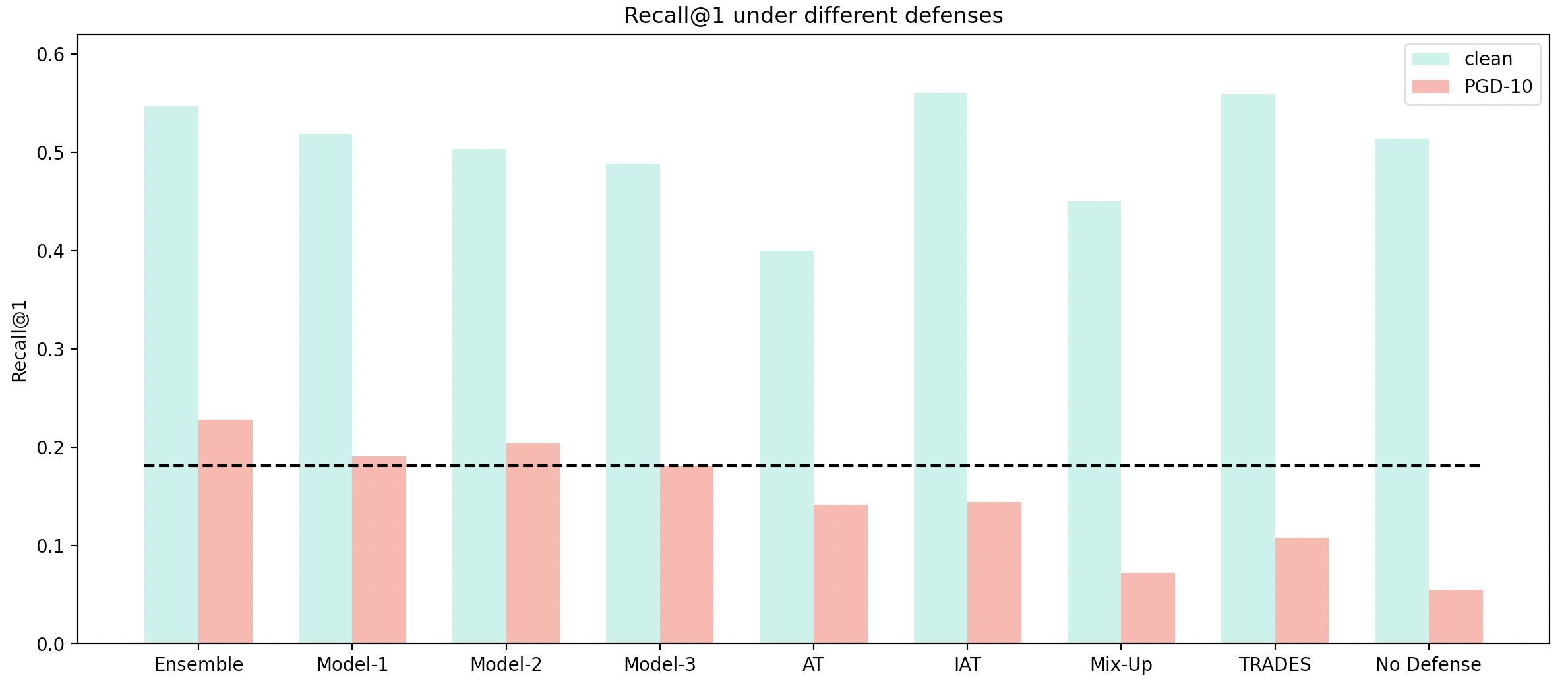
Figure 5: Recall@1 for the individual model of the EAT defense in comparison with other defenses on the CUB200 dataset (Training with the MobileNetV2)

Ablation Study

The comparison of the Naive Ensemble Method As is shown in the Table 3, we perform the naive ensemble method (i.e. Training three models individually and construct a simple ensemble through the vote mechanism) on the CUB200 dataset. Our EAT method presents better robustness than the naive ensemble method.

The robustness gain of the split mechanism As is shown in the Table 3, we also analyze the gain of our split mechanism. Our split mechanism brings the 9.13% robustness improvement on the CUB200 dataset.

Method NMI F1-Score Recall@1 Recall@8 Naive Ensemble Clean 58.95 20.93 53.47 81.76 PGD-10 34.76 3.26 17.91 40.91 EAT w/o Data Split Clean 59.28 21.25 54.49 82.02 PGD-10 36.13 4.23 21.46 45.25 EAT w/ Data Split Clean 56.91 19.28 52.78 80.48 PGD-10 38.02 4.84 24.02 47.49

Table 3: The ablation experiment on the CUB200 with the MobileNetV2 under for presenting the benefit of the split mechanism.

Method NMI F1-Score Recall@1 Recall@10 Recall@20 PAL Clean 86.88 14.95 60.97 82.69 86.70 PGD-10 82.47 3.36 16.25 32.86 39.05 PAL + AT Clean 86.71 14.19 57.29 80.41 84.79 PGD-10 84.68 8.51 38.06 62.46 69.20 PAL + Mix-Up Clean 86.88 14.85 60.77 82.75 86.68 PGD-10 82.46 3.43 16.66 33.44 39.53 PAL + IAT Clean 86.76 14.37 57.98 80.86 85.54 PGD-10 84.78 8.80 38.27 63.03 69.72 PAL+TRADES Clean 87.35 16.18 63.37 84.61 88.37 PGD-10 81.95 2.45 11.36 24.38 28.99 PAL + EAT Clean 86.82 14.40 58.69 79.58 84.34 PGD-10 85.30 10.03 43.16 66.16 72.64

Table 4: The comparison of five defenses on the In-Shop with the MobileNetV2 under the white-box adversarial example attack.

Conclusion

In this work, we analyze the adversarial robustness in DML under the adversarial example attacks. We find that some popular defenses (Mix-Up, IAT and TRADES) fail on the DML tasks and the traditional AT defense also works not so well. To alleviate the effect of the adversarial examples, we propose the Ensemble Adversarial Training (EAT) defense by promoting the diversity of the ensemble and constructing the self-transferring mechanism for further improving the adversarial robustness of the ensemble. We implement and evaluate our EAT defense on three popular datasets (CUB200, CARS196, and In-Shop). Our experiments show the EAT defense outperforms other defenses which have been used on the classification tasks. Furthermore, we make the ablation study to better understand the gain of our split mechanism and the whole EAT defense.