Efficient Connectivity-Preserving Instance Segmentation
with Supervoxel-Based Loss Function

Abstract

Reconstructing the intricate local morphology of neurons and their long-range projecting axons can address many connectivity related questions in neuroscience. The main bottleneck in connectomics pipelines is correcting topological errors, as multiple entangled neuronal arbors is a challenging instance segmentation problem. More broadly, segmentation of curvilinear, filamentous structures continues to pose significant challenges. To address this problem, we extend the notion of simple points from digital topology to connected sets of voxels (i.e. supervoxels) and propose a topology-aware neural network segmentation method with minimal computational overhead. We demonstrate its effectiveness on a new public dataset of 3-d light microscopy images of mouse brains, along with the benchmark datasets DRIVE, ISBI12, and CrackTree.

Introduction

High-throughput neuron reconstruction is a challenging 3-d instance segmentation problem and a major bottleneck of many data-driven neuroscience studies (Gouwens et al. 2020; Winnubst et al. 2019). Deep learning-based methods are the leading framework for segmenting individual neurons, which is a critical step in reconstructing neural circuits (Turaga et al. 2010; Januszewski et al. 2018; Lee et al. 2019; Schmidt et al. 2024). While these methods and many others have significantly improved segmentation quality, automated reconstruction of neurons from large 3-d images still suffers from topological errors (i.e. splits and merges) and requires substantial human proofreading. This can be attributed to two basic observations: (i) neuronal branches can be as thin as a single voxel and (ii) branches often touch or even overlap due to the imaging resolution. Consequently, a seemingly innocuous mistake at the single voxel level can produce catastrophically incorrect segmentations.

A natural solution to these challenges is to account for the topology of the underlying objects during training. Several methods use persistent homology to capture the topology of segmented objects in terms of their Betti numbers (Clough et al. 2019; Hu et al. 2021; Stucki et al. 2023). While these methods have achieved state-of-the-art results, they are computationally expensive with complexities that scale nonlinearly. In this paper, we present a more efficient approach based on an extension of simple voxels from digital topology. Our method aims to preserve the connectivity of segmented objects and has significantly faster training times that scale linearly.

In digital topology, a simple point in a 3-d binary image is defined as a foreground voxel whose deletion does not change the topology of the image (Kong and Rosenfeld 1989). Specifically, deleting a simple voxel does not result in splits or merges, nor does it create or eliminate loops, holes, or objects. This concept has been used to penalize errors involving non-simple voxels when segmenting neurons (Gornet et al. 2019). However, topological errors often involve multiple connected voxels, which is not addressed by a single voxel-based approach.

To overcome this limitation, we extend the concept of simple voxels to supervoxels (i.e., connected sets of voxels). We then propose a differentiable loss function based on this supervoxel characterization, which enables neural networks to be trained to minimize split and merge errors. Finally, we evaluate our approach on 3-d light microscopy images of mouse brains as well as on several 2-d segmentation datasets.

Related Works

Accurately segmenting fine-scale structures such as neurons, vessels, and roads from satellite images is a complex and well-studied problem. There are two general approaches: (1) improve feature representations (e.g., (Wu et al. 2017; Mosinska et al. 2018; Hu et al. 2023; Sheridan et al. 2023)) and (2) incorporate topology-inspired loss functions during training. The latter approach focuses on identifying critical locations where the neural network is prone to topological errors, and then using gradient-based updates to guide improvements.

Bertrand and Malandain (1994) studied topological characterization of simple voxels. The astonishing success of this work is that a complete topological description of a voxel can be derived through basic operations on its immediate neighborhood. Notably, this study does not invoke modern topological concepts such as homology or Morse theory to characterize voxels in low-dimensional digital topology. In many ways, the present study is inspired by that work.

The method most closely related to ours is centerlineDice (clDice), which is also a connectivity-aware loss function (Shit et al. 2021). In this approach, soft skeletons of both the prediction and ground truth are generated by applying min- and max-pooling $k$ times during training. The loss is then computed by evaluating the overlap between the segmented objects and skeletons. Similar to our method, clDice also preserves topology up to homotopy equivalence – if the hyperparameter $k$ is greater than the maximum observed radius.

Recently, persistent homology has been used in deep learning frameworks to track higher-order topological structures during training (Hofer et al. 2017, 2019; Chen et al. 2019; Stucki et al. 2023). Clough et al. (2019) used the Betti numbers of the ground truth as a topological prior and computed gradients to adjust the persistence of topological features. Hu et al. (2019) introduced a penalty for discrepancies between persistence diagrams of the prediction and ground truth. More recently, Hu et al. (2021) used discrete Morse theory to identify topologically significant structures and employed persistence-based pruning to refine them.

Turaga et al. (2009) introduced MALIS for affinity-based models to improve the predictions at maximin edges. This method involves costly gradient updates requiring a maximin search to identify voxels most likely to cause topological errors. Funke et al. (2018) introduced constrained MALIS to improve computational efficiency by computing gradients in two separate passes: one for affinities within ground truth objects and another for affinities between and outside these objects.

Several studies have leveraged the concept of non-simple voxels to develop topology-aware segmentation methods. Gornet et al. (2019) improved neuron segmentation by penalizing errors at non-simple voxels. Additionally, homotopy warping has been used to prioritize errors at non-simple voxels over minor boundary discrepancies (Jain et al. 2010; Hu 2022). However, these approaches are computationally expensive since they require voxel-by-voxel analysis to detect non-simple voxels in each prediction.

Method

Let $G=(V,E)$ be an undirected graph with the vertex set $V=\{1,\ldots,n\}$. We assume that $G$ is a graphical representation of an image where the vertices represent voxels and edges are defined with respect to a $k$-connectivity constraint. A ground truth segmentation $y=(y_{1},\ldots,y_{n})$ is a labeling of the vertices with $y_{i}\in\{0,\ldots,m\}$. We assume $\hat{y}=(\hat{y}_{1},\ldots,\hat{y}_{n})$ denotes a prediction of the ground truth.

Let $F(y)=\{i\in V:y_{i}\neq 0\}$ be the foreground of the vertex labeling, which may include multiple and potentially touching objects. Let $\mathcal{S}(y)\subseteq\mathscr{P}(V)$ be the set of connected components induced by the labeling $y$, where $\mathscr{P}(V)$ is the power set of $V$.

In a labeled graph, the connected components are determined by the equivalence relation that $i\sim j$ if and only if $y_{i}=y_{j}$ with $i,j\in F(y)$ and there exists a path from $i$ to $j$ that is entirely contained within the same segment. An equivalence relation induces a partition over a set into equivalence classes that correspond to the connected components in this setting.

We propose a novel connectivity-preserving loss function to train topology-aware neural networks with the goal of avoiding false splits of, and false merges between foreground objects.

Definition 1.

Let $\mathcal{L}:\mathbb{R}^{n}\times\mathbb{R}^{n}\rightarrow\mathbb{R}$ be the loss function given by

$$\mathcal{L}(y,\hat{y}) =(1-\alpha)\,\mathcal{L}_{0}(y,\hat{y})+\alpha\,\beta\sum_{C\in\mathcal{P}(\hat{y}_{+})}\mathcal{L}_{0}(y_{C},\hat{y}_{C})$$

$$+\alpha\,(1-\beta)\sum_{C\in\mathcal{N}(\hat{y})}\mathcal{L}_{0}(y_{C},\hat{y}_{C})$$

such that $\alpha,\beta\in[0,1]$ and $\mathcal{L}_{0}$ is an arbitrary loss function.

We build upon a traditional loss function $\mathcal{L}_{0}$ (e.g. cross-entropy or Dice coefficient) by incorporating additional terms that penalize sets of connected voxels (i.e. supervoxels) responsible for connectivity errors. These supervoxels are identified by analyzing connected components in the false negative and false positive masks, which are obtained by comparing the foregrounds of $y$ and $\hat{y}$

The sets $\mathcal{N}(\hat{y})$ and $\mathcal{P}(\hat{y}_{+})$ consist of connected components whose addition or removal changes the number of connected components. A component that changes the underlying topology in this manner is called a critical component. Next, we rigorously define this notion, and present an algorithm for detecting critical components.

Critical Components

Critical components generalize the notion of non-simple voxels from digital topology to supervoxels. In digital topology, a voxel is called non-simple if its addition or removal changes the number of connected components, holes, or cavities. Similarly, a supervoxel is called critical if its addition or removal changes the number of connected components. We use the term critical as opposed to non-simple because the definition is not a direct generalization for computational reasons. This more focused definition enables our supervoxel-based loss function to be computed in linear time, which is a significant improvement over existing topological loss functions.

False Splits

Let $\hat{y}$ be the false negative mask determined by comparing a prediction to the ground truth. Let $\mathcal{S}_{y}(\hat{y})$ be the set of connected components of $\hat{y}$ with respect to $y$. The connected components in this set are defined by the following criteria: two voxels $i\sim j$ are part of the same component if:

• $(\hat{y})_{i}=(\hat{y})_{j}$ with $i,j\in F(\hat{y})$

• $y_{i}=y_{j}$

• There exists a path from $i$ to $j$ contained within the same segments.

This second condition ensures that each component in the false negative mask corresponds precisely to one connected component in the ground truth.

Negatively critical components are determined by comparing the number of connected components in $y$ and $y\ominus C$ such that $C\in\mathcal{S}_{y}(\hat{y})$. The notation $y\ominus C$ denotes “removing” a component from the ground truth. The result of this operation is a vertex labeling where the label of node $i\in V$ is given by

$$(y\ominus C)_{i}=\begin{cases}0,&\text{if }i\in C\\ y_{i},&\text{otherwise }\\ \end{cases}$$ (1)

The removal of a component only impacts a specific region within the graph; the component itself and the nodes connected to its boundary. Thus, for topological characterization, it is sufficient to check whether its removal changes the number of connected components in that local region instead of the entire graph. Let $N(C)\subseteq V$ be the neighborhood surrounding a component $C\in\mathcal{S}(y)$ such that $N(C)=\{i\in V:\{i,j\}\in E\text{ and }j\in C\}$. Let $y\cap N(C)$ represent the labeling $y$ within $N(C)$.

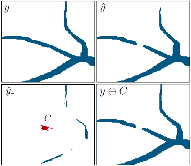
Figure 1: Top: Image patches of ground truth and predicted segmentations. Bottom: False negative mask with the component $C$ highlighted in red. $C$ is negatively critical since its removal changes the connectivity of the ground truth.

Definition 2.

A component $C\in\mathcal{S}_{y}(\hat{y})$ is said to be negatively critical if $|\mathcal{S}\big{(}y\cap N(C)\big{)}|\neq|\mathcal{S}\big{(}(y\ominus C)\cap N(C)\big{)}|$.

Negatively critical components change the local topology by either deleting an entire component or altering the connectivity between vertices in $N(C)$ from the ground truth. In the latter case, the removal of such components locally disconnects some $i,j\in N(C)$ so that it is impossible to find a path (in this neighborhood) that does not pass through $C$. Based on this intuition, we can establish an equivalent definition of negatively critical components as components that are either (1) identical to a component in the ground truth or (2) locally disconnect at least one pair of nodes in $N(C)$ after being removed.

Theorem 1.

A component $C\in\mathcal{S}_{y}(\hat{y})$ is negatively critical if and only if there exists an $A\in\mathcal{S}(y\cap N(C))$ with $A\supseteq C$ such that either $(1)$ $A=C$ or $(2)$ $\exists\,v_{0},v_{k}\in A\setminus C$ such that there does not exist a path $(v_{0},\ldots,v_{k})\subseteq N(C)$ with $v_{i}\notin C$ for $i=1,\ldots,k-1$. (Proof is in the Appendix.)

One computational challenge in both characterizations is the need to recompute connected components within the neighborhood $N(C)$ for every $C\in\mathcal{S}_{y}(\hat{y})$. In the worst case, the complexity is $\mathcal{O}(n^{2})$ with respect to the number of voxels in the image. However, we can develop a more efficient algorithm with $\mathcal{O}(n)$ complexity by leveraging two useful facts: (i) neurons are tree-structured objects, implying that, (ii) negatively critical components change both the local and global topology.

Recall that a negatively critical component $C\in\mathcal{S}_{y}(\hat{y})$ changes the local topology of $N(C)$ in the sense that $|\mathcal{S}\big{(}y\cap N(C)\big{)}|\neq|\mathcal{S}\big{(}(y\ominus C)\cap N(C)\big{)}|$. Analogously, $C$ also changes the global topology if $|\mathcal{S}(y)|\neq|\mathcal{S}(y\ominus C)|$. In this special case, we can establish an equivalent definition, similar to Theorem 1, that utilizes $\mathcal{S}(y)$ and $\mathcal{S}(y\ominus C)$ in place of $\mathcal{S}(y\cap N(C))$ and $\mathcal{S}((y\ominus C)\cap N(C))$.

This characterization can be further simplified by using $\mathcal{S}(y\ominus\hat{y})$ instead of $\mathcal{S}(y\ominus C)$, where $y\ominus\hat{y}$ represents the ground truth after removing all components in the false negative mask:

$$(y\ominus\hat{y})_{i}=\begin{cases}0,&\text{if }(\hat{y})_{i}=1\\ y_{i},&\text{otherwise }\\ \end{cases}$$

Note that this characterization is the key to overcoming nonlinear computational complexity.

Corollary 1.

A component $C\in\mathcal{S}_{y}(\hat{y})$ is negatively critical with $|\mathcal{S}(y)|\neq|\mathcal{S}(y\ominus C)|$ if and only if there exists an $A\in\mathcal{S}(y)$ with $A\supseteq C$ such that either $(1)$ $A=C$ or $(2)$ $\exists B_{1},B_{2}\in\mathcal{S}(y\ominus\hat{y})$ with $B_{1},B_{2}\subset A$ such that $B_{1}\cup C\cup B_{2}$ is connected. (Proof is in the Appendix.)

False Merges

Let $\hat{y}_{+}$ be the false positive mask determined by comparing the prediction to the ground truth. Analogously, a component in the false positive mask is positively critical if its addition to the ground truth changes the number of connected components in the immediate neighborhood. While this notion can be articulated, for consistency and to leverage previous results, we opt for an equivalent formulation. Alternatively, a component in the false positive mask is positively critical if its removal from the predicted segmentation changes the topology.

Definition 3.

A component $C\in\mathcal{S}_{y}(\hat{y}_{+})$ is said to be positively critical if $|\mathcal{S}(\hat{y}\cap N(C))|\neq|\mathcal{S}(\hat{y}\ominus C\cap N(C))|$.

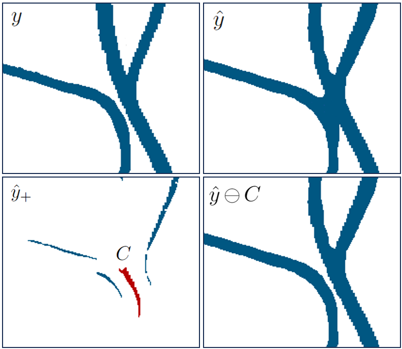
Figure 2: Top: Image patches of ground truth and predicted segmentations. Bottom: False positive mask with a single component $C$ highlighted. $C$ is positively critical since its removal changes the number of connected components.

Positively critical components change the local topology by either (1) creating a component or (2) altering the connectivity between ground truth objects. In the latter, these components connect pairs of nodes that belong to locally distinct components. Equivalently, their removal causes pairs of nodes to become locally disconnected. Next, we present an equivalent definition that characterizes positively critical components as satisfying one of these conditions.

Theorem 2.

A component $C\in\mathcal{S}_{y}(\hat{y}_{+})$ is positively critical if and only if there exists an $A\in\mathcal{S}(\hat{y})$ with $A\supseteq C$ such that either $(1)$ $A=C$ or $(2)$ $\exists\,v_{0},v_{k}\in A\setminus C$ such that there does not exist a path $(v_{0},\ldots,v_{k})\subseteq N(C)$ with $v_{i}\notin C$ for $i=1,\ldots,k-1$. (Proof is in the Appendix.)

Similarly, positively critical components present the same computational challenge of needing to recompute connected components for every $C\in\mathcal{S}_{y}(\hat{y}_{+})$. However, we can avoid this expensive calculation by utilizing a corollary of Theorem 2 that establishes an equivalent definition of positively critical components that also change the global topology. This characterization uses $\mathcal{S}(\hat{y})$ and $\mathcal{S}(\hat{y}\ominus\hat{y}_{+})$, instead of $\mathcal{S}(y\cap N(C))$ and $\mathcal{S}((\hat{y}\ominus C)\cap N(C))$, where $\hat{y}\ominus\hat{y}_{+}$ denotes removing every component in the false positive mask from the prediction via

$$(\hat{y}\ominus\hat{y}_{+})_{i}=\begin{cases}0,&\text{if }(\hat{y}_{+})_{i}=1\\ \hat{y}_{i},&\text{otherwise }\\ \end{cases}$$

Corollary 2.

A component $C\in\mathcal{S}_{y}(\hat{y}_{+})$ is positively critical with $|\mathcal{S}(\hat{y})|\neq|\mathcal{S}(\hat{y}\ominus C)|$ if and only if there exists an $A\in\mathcal{S}(\hat{y})$ with $A\supseteq C$ such that either $(1)$ $A=C$ or $(2)$ $\exists B_{1},B_{2}\in\mathcal{S}(\hat{y}\ominus\hat{y}_{+})$ with $B_{1},B_{2}\subset A$ such that $B_{1}\cup C\cup B_{2}$ is connected. (Proof is in the Appendix.)

Computing Critical Components

Although topological loss functions improve segmentation accuracy, one major drawback is that they are computationally expensive. A key advantage of our proposed method is that the runtime is $\mathcal{O}(n)$ with respect to the number of voxels. In contrast, related methods have either $\mathcal{O}(n\log n)$ or $\mathcal{O}(n^{2})$ complexity (e.g. Turaga et al. (2009); Gornet et al. (2019); Hu et al. (2021); Shit et al. (2021); Hu et al. (2023)).

In the case of identifying non-simple voxels, Bertrand and Malandain (1994) proved that it is sufficient to examine the topology of the neighborhood. Similarly, we can determine whether a component is critical by checking the topology of nodes connected to the boundary. For the remainder of this section, we focus the discussion on computing negatively critical components since the same algorithm can be used to compute positively critical components.

Let $D(C)=N(C)\setminus C$ be the set of nodes connected to the boundary of a component $C\in\mathcal{S}_{y}(\hat{y})$. Assuming that a negatively critical component also changes the global topology, Corollary 1 can be used to establish analogous conditions on the set $D(C)$ that are useful for fast computation.

Corollary 3.

A component $C\in\mathcal{S}_{y}(\hat{y})$ is negatively critical with $|\mathcal{S}(y)|\neq|\mathcal{S}(y\ominus C)|$ if and only if $\exists A\in\mathcal{S}(y)$ with $A\supseteq C$ such that either $(1)$ $\nexists\,i\in D(C)$ with $i\in A$ or $(2)$ $\exists B_{1},B_{2}\in\mathcal{S}(y\ominus\hat{y})$ with $B_{1},B_{2}\subset A$ such that $i\in B_{1}$ and $j\in B_{2}$ for some $i,j\in D(C)$. (Proof is in the Appendix.)

The key to achieving linear complexity is to precompute $\mathcal{S}(y)$ and $\mathcal{S}(y\ominus\hat{y})$, then use a breadth-first search (BFS) to compute $\mathcal{S}_{y}(\hat{y})$ while simultaneously checking Conditions 1 and 2. Intuitively, the core idea is that once this BFS reaches the boundary of the component, we can visit all nodes in $D(C)$ and efficiently check the conditions.

Let $r\in F(\hat{y})$ be the root of the BFS. Given a node $j\in D(C)$, Conditions 1 and 2 can be efficiently checked using a hash table that stores the connected component label of $j$ in $\mathcal{S}(y)$ and $\mathcal{S}(y\ominus\hat{y})$ as a key-value pair. If we never visit a node $j\in D(C)$ with the same ground truth label as the root, then this label is not a key in the hash table and the component satisfies Condition 1 (Line 19, Algo. 2).

Now consider the case where we visit a node $j\in D(C)$ with the same ground truth label as the root. If the label of $j$ in $\mathcal{S}(y)$ is not already a key in the hash table, a new entry is created (Line 15, Algo. 2). Otherwise, the value corresponding to this key is compared to the label of $j$ in $\mathcal{S}(y\ominus\hat{y})$. If they differ, then the component satisfies Condition 2.

Note that pseudocode for this method is provided in Algo. 1 and 2 and our code is publicly available at https://github.com/AllenNeuralDynamics/supervoxel-loss.

Theorem 3.

The computational complexity of computing critical components that satisfy either $|\mathcal{S}(y)|\neq|\mathcal{S}(y\ominus C)|$ or $|\mathcal{S}(\hat{y})|\neq|\mathcal{S}(\hat{y}\ominus C)|$ is $\mathcal{O}(n)$ with respect to the number of voxels in the image. (Proof is in the Appendix.)

We emphasize that the statements and algorithms surrounding Theorem 3 are restricted to tree-structured objects (i.e. critical components that satisfy $|\mathcal{S}(y)|\neq|\mathcal{S}(y\ominus C)|$ or $|\mathcal{S}(\hat{y})|\neq|\mathcal{S}(\hat{y}\ominus C)|$). Indeed, a similar algorithm based on the main definitions and deductions can be implemented in a straightforward manner for the general case, except that this algorithm will be super-linear in complexity.

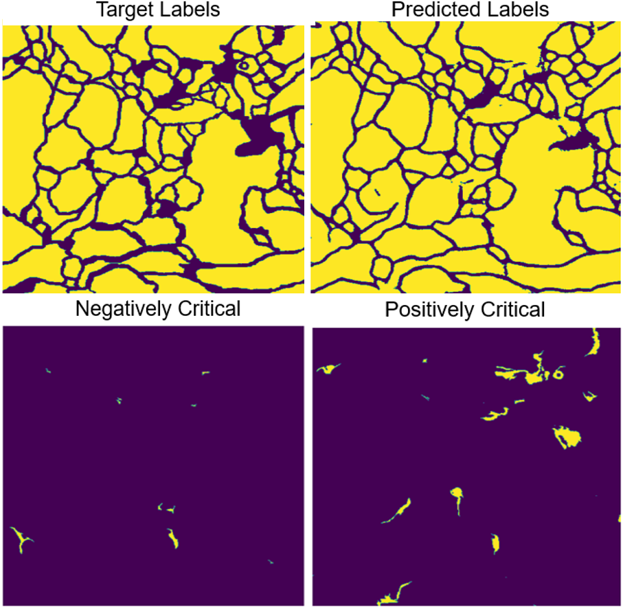
Figure 3: Segmentation of a 512x512 image from the ISBI12 dataset. The critical components of this prediction were computed in 1.41 seconds using code at https://github.com/AllenNeuralDynamics/supervoxel-loss.

Penalizing Critical Topological Mistakes

Our topological loss function builds upon classical, voxel-based loss functions by adding terms that penalize critical components. The paradigm shift here is to evaluate each mistake at a “structure level” that transcends rectilinear geometry, as opposed to the voxel level, without resorting to expensive search iterations. In standard loss functions, mistakes are detected at the voxel-level by directly comparing the prediction at each voxel against the ground truth. Instead, we consider the context of each mistake by determining whether a given supervoxel causes a critical topological mistake.

The hyperparameter $\alpha\in[0,1]$ is a scaling factor that controls the relative importance of voxel-level versus structure-level mistakes. Similarly, $\beta\in[0,1]$ controls the weight placed on split versus merge mistakes. In situations where false merges are more costly or time-consuming to correct manually, $\beta$ can be set to a value greater than 0.5 to prioritize preventing merge errors by assigning them higher penalties.

Our topological loss function is architecture agnostic and can be easily integrated into existing deep learning pipelines. We recommend training a baseline model with a standard loss function, then fine-tuning with the topological loss function. This topological function adds little computational overhead since the only additional calculation is to compute the critical components. In Theorem 3, we prove that Algorithms 1 and 2 can be used to compute critical components in linear time. This result can then be used to show that the computational complexity of computing our proposed topological loss function is also $\mathcal{O}(n)$ in the number of voxels in the image.

Experiments

We evaluate our method on the following image segmentation datasets: DRIVE, ISBI12, CrackTree and EXASPIM. DRIVE is a retinal vessel dataset consisting of 20 images with dimensions 584x565 (Staal et al. 2004). ISBI12 is an electron microscopy (EM) dataset consisting of 29 images with dimensions 512x512. CrackTree contains 206 images of cracks in roads, where the size of each image is 600x800. EXASPIM is a 3-d light sheet microscopy dataset consisting of 37 images whose dimensions range from 256x256x256 to 1024x1024x1024 and voxel size is $\sim$$1\text{\,}\mathrm{\SIUnitSymbolMicro m}$³ (Glaser et al. 2024).

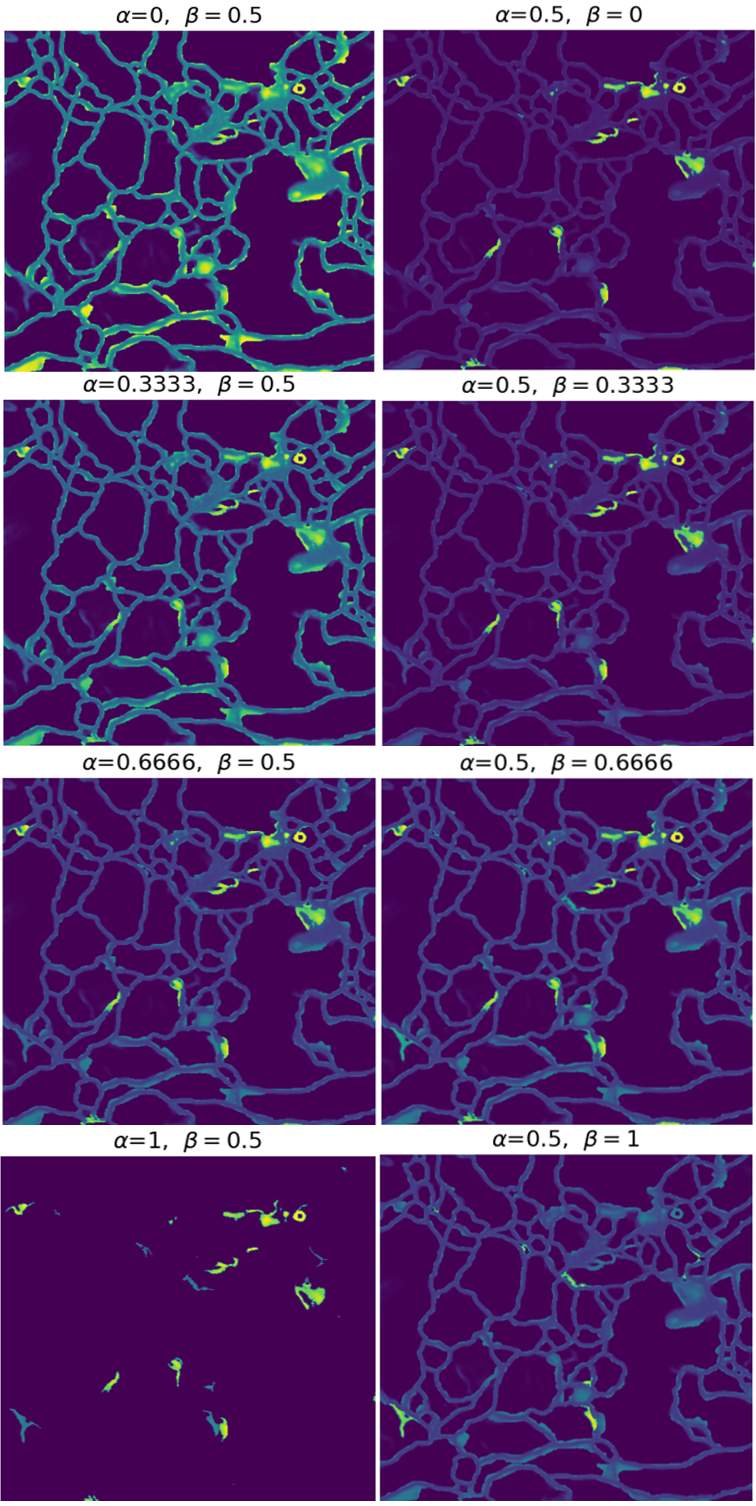
Figure 4: Visualization of the loss in the prediction in Fig. 3. Left: As $\alpha$ varies from 0 to 1, the loss places higher penalties on critical components. Right: As $\beta$ varies from 0 to 1, the loss shifts from assigning higher penalties to negatively critical to positively critically components.

For the 2-d datasets, we perform 3-fold cross-validation for each method and report the mean and standard deviation across the validation set. For the 3-d dataset, we evaluate the methods on a test set consisting of 4 images. In all experiments, we set $\alpha=0.5$ and $\beta=0.5$ in our proposed topological loss function.

Evaluation Metrics. We use four evaluation metrics: pixel-wise accuracy, Dice coefficient, Adjusted Rand Index (ARI), Variation of Information (VOI) and Betti number error. The last three metrics are more topology-relevant in the sense that small topological differences can lead to significant changes in the error. See the Appendix for additional details on each metrics.

Baselines. For the 2-d datasets, we compare our method to U-Net (Ronneberger, Fischer, and Brox 2015), Dive (Fakhry, Peng, and Ji 2016), Mosin. (Mosinska et al. 2018), TopoLoss (Hu et al. 2019), and DMT (Hu et al. 2023). For the 3-d datasets, we compare our method to U-Net (Ronneberger, Fischer, and Brox 2015), Gornet (Gornet et al. 2019), clDice (Shit et al. 2021), and MALIS (Turaga et al. 2009). For the 2-d datasets, the segmentations were generated by applying a threshold of 0.5 to the predicted likelihoods. For the 3-d dataset, where some objects are touching, the segmentations were generated by applying a watershed algorithm to the prediction (Zlateski and Seung 2015).

Results. Table 1 shows quantitative results for the different models on the segmentation datasets. Our proposed method achieves state-of-the-art results; particularly, for the topologically relevant metrics. Figures 5 and 6 (full raw images and segmentations in the Appendix) present qualitative results that visually compare the performance of U-Net models trained with cross-entropy versus our proposed loss function. Although the only difference between these two models is the addition of topological terms, there is a clear difference in topological accuracy.

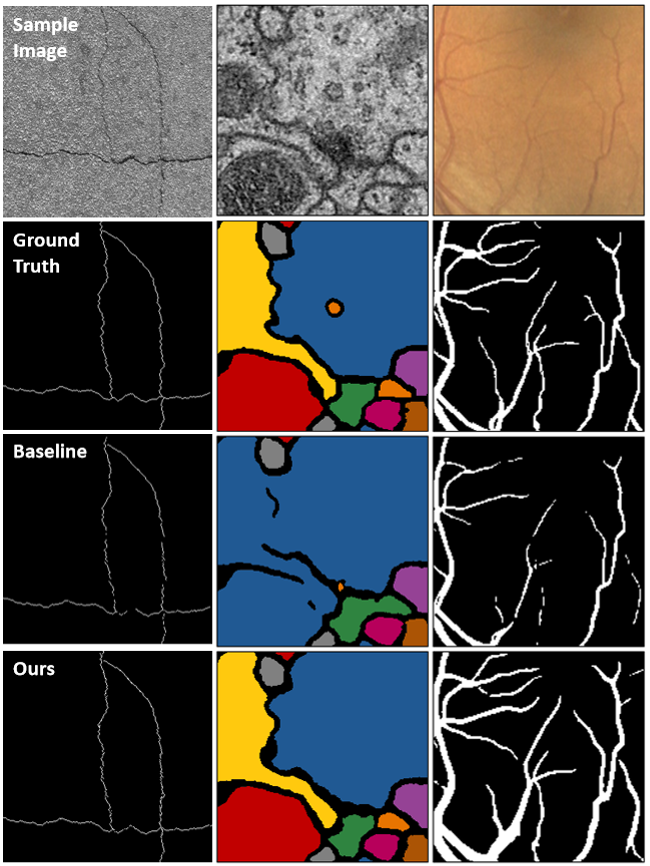
Figure 5: Qualitative results on three 2d datasets.

Table 1: Quantitative results for different models on several datasets. Results for Dive, Mosin., TopoLoss, and DMT are from (Hu et al. 2023). $\mathcal{O}(\cdot)$: complexity of training iterations, $n$: number of pixels/voxels, $k$: number of pooling operations in clDice.

Method	$\mathcal{O}(\cdot)$	Dice $\uparrow$	ARI $\uparrow$	VOI $\downarrow$	Betti Error $\downarrow$
DRIVE
U-Net	$n$	0.749$\pm$0.003	0.834$\pm$0.041	1.98$\pm$0.05	3.64$\pm$0.54
DIVE	$n$	0.754$\pm$0.001	0.841$\pm$0.026	1.94$\pm$0.13	3.28$\pm$0.64
Mosin.	$n$	0.722$\pm$0.001	0.887$\pm$0.039	1.17$\pm$0.03	2.78$\pm$0.29
TopoLoss	$n\log n$	0.762$\pm$0.004	0.902$\pm$0.011	1.08$\pm$0.01	1.08$\pm$0.27
DMT	$n^{2}$	0.773$\pm$0.004	0.902$\pm$0.002	0.88$\pm$0.04	0.87$\pm$0.40
Ours	$n$	0.809$\pm$0.012	0.943$\pm$0.002	0.48$\pm$0.01	0.94$\pm$0.27
ISBI12
U-Net	$n$	0.970$\pm$0.005	0.934$\pm$0.007	1.37$\pm$0.03	2.79$\pm$0.27
DIVE	$n$	0.971$\pm$0.003	0.943$\pm$0.009	1.24$\pm$0.03	3.19$\pm$0.31
Mosin.	$n$	0.972$\pm$0.002	0.931$\pm$0.005	0.98$\pm$0.04	1.24$\pm$0.25
TopoLoss	$n\log n$	0.976$\pm$0.004	0.944$\pm$0.008	0.78$\pm$0.02	0.43$\pm$0.10
DMT	$n^{2}$	0.980$\pm$0.003	0.953$\pm$0.005	0.67$\pm$0.03	0.39$\pm$0.11
Ours	$n$	0.983$\pm$0.001	0.934$\pm$0.001	0.74$\pm$0.03	0.48$\pm$0.02
CrackTree
U-Net	$n$	0.649$\pm$0.003	0.875$\pm$0.042	1.63$\pm$0.10	1.79$\pm$0.30
DIVE	$n$	0.653$\pm$0.002	0.863$\pm$0.0376	1.57$\pm$0.08	1.58$\pm$0.29
Mosin.	$n$	0.653$\pm$0.001	0.890$\pm$0.020	1.11$\pm$0.06	1.05$\pm$0.21
TopoLoss	$n\log n$	0.673$\pm$0.004	0.929$\pm$0.012	0.99$\pm$0.01	0.67$\pm$0.18
DMT	$n^{2}$	0.681$\pm$0.005	0.931$\pm$0.017	0.90$\pm$0.08	0.52$\pm$0.19
Ours	$n$	0.667$\pm$0.010	0.914$\pm$0.011	0.98$\pm$0.10	0.51$\pm$0.06
EXASPIM
U-Net	$n$	0.751$\pm$0.047	0.875$\pm$0.082	1.28$\pm$0.46	0.74$\pm$0.03
Gornet	$n^{2}$	0.777$\pm$0.083	0.901$\pm$0.049	0.65$\pm$0.17	0.42$\pm$0.07
clDice	$kn$	0.785$\pm$0.032	0.923$\pm$0.071	0.66$\pm$0.51	0.36$\pm$0.07
MALIS	$n^{2}$	0.794$\pm$0.052	0.927$\pm$0.042	0.64$\pm$0.27	0.34$\pm$0.08
Ours	$n$	0.770$\pm$0.058	0.953$\pm$0.038	0.42$\pm$0.21	0.31$\pm$0.06

Evaluation with Skeleton-Based Metrics. Although the performance of segmentation models is typically evaluated using voxel-based metrics, such as those in Table 1, skeleton-based metrics are better suited to evaluate neuron segmentations. This is because the main objective of this task is to reconstruct the morphology of individual neurons and their interconnectivity. Thus, skeleton-based metrics are preferable because they quantify to what extent the topological structure of a neuron was accurately reconstructed.

In this evaluation, we compare a set of ground truth skeletons to the predicted segmentations to compute the following metrics: number of splits/neuron (Splits$/$Neuron), edge accuracy, and normalized expected run length (ERL) (see the Appendix for definitions). The number of merges per neuron was also computed, but the watershed parameters were configured to prevent merges in the segmentations.

Table 2 presents quantitative results for the different models on the EXASPIM dataset. These results show that our proposed method achieves the highest topological accuracy. In particular, our proposed method has the best normalized ERL, which is regarded as the gold standard for evaluating the accuracy of a neuron’s topological reconstruction (Januszewski et al. 2018). Perhaps as importantly, our method scales linearly and achieves favorable runtimes, consistent with Thm. 3 (see Tables 2 and 4).

Table 2: Skeleton-based metrics for different models for the EXASPIM dataset.

Method	Complexity	Runtime$/$Epoch $\downarrow$	Splits$/$Neuron $\downarrow$	Edge Accuracy $\uparrow$	Normalized ERL $\uparrow$
U-Net	$\mathcal{O}(n)$	10.03$\pm$0.23 sec	9.86$\pm$13.30	0.873$\pm$0.087	0.596$\pm$0.232
Gornet	$\mathcal{O}(n^{2})$	71.62$\pm$1.83 sec	3.85$\pm$2.58	0.937$\pm$0.062	0.664$\pm$0.106
clDice	$\mathcal{O}(kn)$	48.55$\pm$1.60 sec	3.39$\pm$1.52	0.911$\pm$0.042	0.701$\pm$0.091
MALIS	$\mathcal{O}(n^{2})$	50.68$\pm$1.58 sec	3.33$\pm$0.59	0.917$\pm$0.053	0.719$\pm$0.098
Ours	$\mathcal{O}(n)$	20.12$\pm$1.15 sec	2.63$\pm$1.36	0.944$\pm$0.043	0.784$\pm$0.099

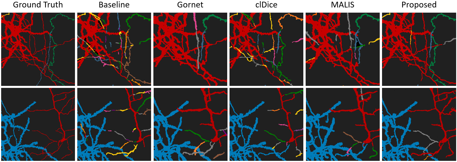
Figure 6: Qualitative results on 3-d EXASPIM dataset. Raw Image: Fig 13

Ablation Study of Hyperparameters. The proposed topological loss function has two interpretable hyperparameters: $\alpha$ and $\beta$. Generally, setting $\alpha$ to a positive value improves the topological accuracy of the segmentation. To better understand their impact on model performance, we performed hyperparameter tuning using Bayesian optimization with the adapted rand index as the objective function (Akiba et al. 2019). We then conducted two separate experiments, where we trained a U-Net using our proposed loss function on both the ISBI12 and EXASPIM datasets.

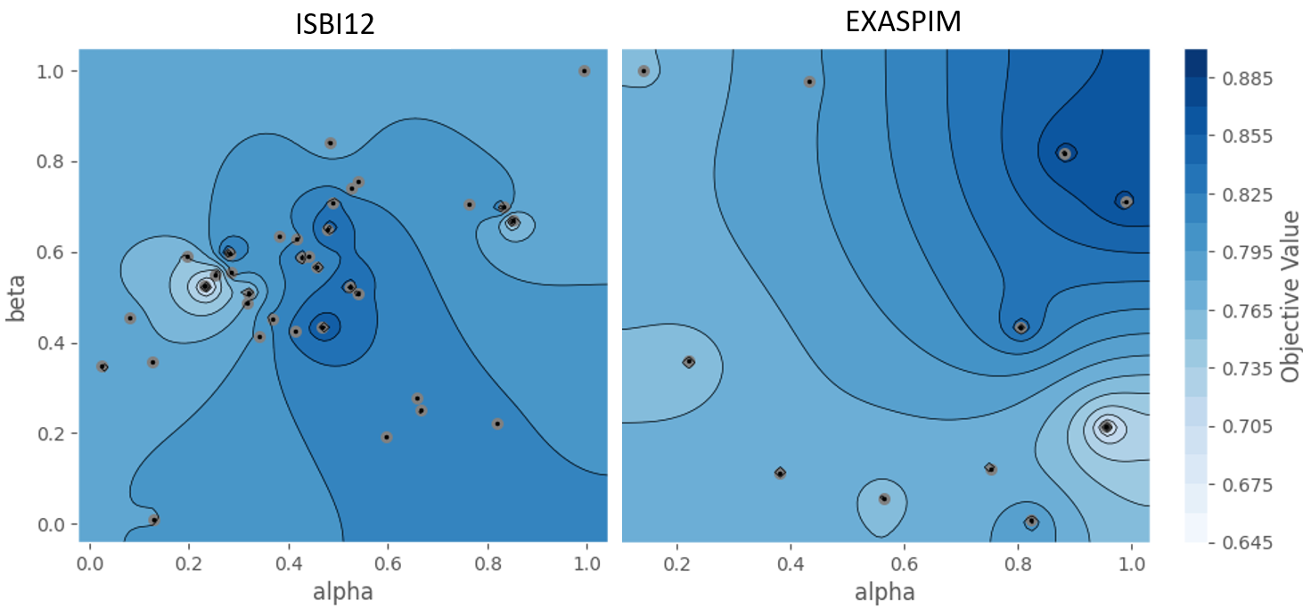
Figure 7: Contour plots of objective functions from hyperparameter optimization, each point is a trial outcome.

Although both datasets consist of neuronal images, they are markedly different: the EXASPIM dataset contains sparse images, while ISBI12 consists of dense ones. Our experiments show that $\alpha\approx 0.5$ and $\beta\approx 0.5$ are optimal for ISBI12, whereas $\alpha\approx 0.9$ and $\beta\approx 0.8$ are optimal for EXASPIM (Fig. 7). A rule of thumb is to set $\alpha,\beta\approx 0.5$ for dense images and increase them together as the image becomes sparser. Notably, Fig. 7 suggests that careful hyperparameter tuning is not critical in practice. In fact, all the results obtained by our method were achieved with a fixed choice for $\alpha$ and $\beta$, without using hyperparameter optimization.

Conclusion

Mistakes that change the connectivity of objects (i.e. topological mistakes) are a key problem in instance segmentation. They produce qualitatively different results based on relatively few pixels/voxels, making it a challenge to avoid such mistakes with voxel-level objectives. Existing work on topology-aware segmentation typically requires costly steps to guide the segmentation towards correct decisions, among other problems.

Here, we generalize the concept of simple voxel to connected components of arbitrary shape, and propose a topology-aware method with minimal computational overhead. We demonstrate the effectiveness of our approach on multiple datasets with different resolutions, dimensionality, and image characteristics. Across multiple metrics, our method achieves state-of-the-art results. It is now possible to image not only a local patch of neuronal morphology, but whole arbors, which can reach multiple, distant brain regions. The favorable scalability of our approach will enable efficient analysis of such large-scale datasets.

Appendix A Characterizations of Critical Components

Given a graph $G=(V,E)$ and vertex labeling $y$, let $\mathcal{S}(y\cap N(C))=\{A_{1},\ldots,A_{m}\}$ be the set of connected components induced by this labeling with $A_{i}\subseteq F(y)$. Let $G^{\prime}=(V^{\prime},E^{\prime})$ be the connected component subgraph with $V^{\prime}=\bigcup_{i=1}^{m}A_{i}$ and $E^{\prime}=\bigcup_{i=1}^{m}E[A_{i}]$ where $E[A_{i}]=\{\{j,k\}\in E:j,k\in A_{i}\}$. Given a subset $U\subseteq V^{\prime}$, the subgraph induced by this set is denoted by $G^{\prime}[U]=(U,E[U])$.

Let $\mu:\mathscr{P}(G)\rightarrow\mathbb{N}$ be a function that counts the number of connected components in $G$, where $\mathscr{P}(G)$ is the set of all subgraphs of $G$. Given $G_{1}=(V_{1},E_{1})$ and $G_{2}=(V_{2},E_{2})$, a disjoint union of these graphs is defined as $G_{1}\cup G_{2}=(V_{1}\cup V_{2},E_{1}\cup E_{2})$.

Lemma 1.

$\mu$ has the following properties:

1. $\mu(G[\varnothing])=0$.

2. Non-negativity. $\mu(G[U])\geq 0$ for all $U\subseteq V$.

3. Finite additivity. For any collection $\{U_{i}\}^{n}_{i=1}$ of pairwise disjoint sets with $U_{i}\subseteq V$,

   $$\mu\Big{(}\bigcup_{i=1}^{n}G[U_{i}]\Big{)}=\sum_{i=1}\mu(G[U_{i}]).$$

Proof.

$\mu(G[\varnothing])=0$ because the empty set does not contain any vertices. This function is non-negative by the definition of connected components. For finite additivity, a disjoint union over pairwise disjoint graphs does not affect the connectivity among vertices. Thus, this property holds by using basic set operations in an inductive argument. ∎

General Case

Lemma 2.

Given a component $C\in\mathcal{S}_{y}(\hat{y})$, there exists a unique $A\in\mathcal{S}(y\cap N(C))$ such that $C\subseteq A$.

Proof.

Choose any $j\in C$, then $y_{j}\neq 0$ by the definition of the false negative mask. Given that $j\in F(y)$, this implies that there exists some $A_{k}\in\mathcal{S}(y)$ with $j\in A_{k}$ and so $C\subseteq\cup_{i=1}^{m}A_{i}$. Using this inclusion, $C$ can be decomposed as

$$C=C\cap\bigcup_{i=1}^{m}A_{i}=\bigcup_{i=1}^{m}C\cap A_{i}.$$

This collection of sets is pairwise disjoint since $\{A_{i}\}_{i=1}^{m}$ is a collection of connected components.

Next, we claim that there exists a unique $A_{k}\in\mathcal{S}(y)$ such that $C\cap A_{k}\neq\varnothing$. By contradiction, suppose there exists a distinct $A_{\ell}\in\mathcal{S}(y)$ with $C\cap A_{\ell}\neq\varnothing$. But this assumption implies the existence of a path between $A_{k}$ and $A_{\ell}$ via $C$ because $C\subseteq F(y\cap N(C))$ implies this set is connected and $C\cap A_{k}\neq\varnothing$ and $C\cap A_{\ell}\neq\varnothing$. Since this contradicts $A_{k}$ and $A_{\ell}$ being disjoint, $A_{k}$ must be unique. Lastly, we can use this uniqueness property to conclude that

$$C=\bigcup_{i=1}^{m}C\cap A_{i}=C\cap A_{k}$$

which implies that $C\subseteq A_{k}$. ∎

Theorem 1.

A component $C\in\mathcal{S}_{y}(\hat{y})$ is negatively critical if and only if there exists an $A\in\mathcal{S}(y\cap N(C))$ with $A\supseteq C$ such that either $(1)$ $A=C$ or $(2)$ $\exists\,v_{0},v_{k}\in A\setminus C$ such that there does not exist a path $(v_{0},\ldots,v_{k})\subseteq N(C)$ with $v_{i}\notin C$ for $i=1,\ldots,k-1$.

Proof.

($\Rightarrow$) Consider the case when $C\in\mathcal{S}_{y}(\hat{y})$ is negatively critical due to $|\mathcal{S}(y\cap N(C))|>|\mathcal{S}((y\ominus C)\cap N(C))|$. Suppose that $\mathcal{S}(y\cap N(C))=\{A_{1},\ldots,A_{m}\}$, then starting from Equation 1 leads to the identity

$$|\mathcal{S}((y\ominus C)\cap N(C))| =\mu\Big{(}\bigcup_{i=1}^{m}G^{\prime}[A_{i}\setminus C]\Big{)}$$

$$=\sum_{i=1}^{m}\mu(G^{\prime}[A_{i}\setminus C])$$

$$=\sum_{\begin{subarray}{c}i=1\\ i\neq j\end{subarray}}^{m}\mu(G^{\prime}[A_{i}])+\mu(G^{\prime}[A_{j}\setminus C])$$

$$=|\mathcal{S}(y\cap N(C))|-1$$

$$\hskip 11.38109pt+\mu(G^{\prime}[A_{j}\setminus C])$$ (2)

where the second equality holds by $\mu$ being a finitely additive function defined over a collection of pairwise disjoint sets by Lemma 1. The third equality holds by using that there exists a unique $A_{j}\in\mathcal{S}(y)$ such that $C\subseteq A_{j}$ by Lemma 2. Under the assumption that $|\mathcal{S}(y\cap N(C))|>|\mathcal{S}((y\ominus C)\cap N(C))|$, it must be the case that $\mu(G^{\prime}[A_{j}\setminus C])=0$. Thus, we have that $A_{j}\setminus C=\varnothing$ which implies $A_{j}\subseteq C$ and so $A_{j}=C$.

Next consider the case when $C\in\mathcal{S}_{y}(\hat{y})$ is negatively critical due to $|\mathcal{S}(y\cap N(C))|<|\mathcal{S}((y\ominus C)\cap N(C))|$. Again using the identity in Equation A, the assumed inequality implies that $\mu(G^{\prime}[A_{j}\setminus C])\geq 2$ and so $G^{\prime}[A_{j}\setminus C]$ must contain at least two connected components. Thus, this set can be decomposed into connected components such that

$$A_{j}\setminus C=\bigcup^{K}_{k=1}B_{k}\subseteq\mathcal{S}((y\ominus C)\cap N(C))$$

with $K\geq 2$. For any $v_{0}\in B_{1}$ and $v_{k}\in B_{2}$, it is impossible to construct a path between these vertices that does not pass through $C$. Otherwise, this would imply that $B_{1}$ and $B_{2}$ are path-connected in the graph $G^{\prime}[A_{j}\setminus C]$ and not distinct connected components.

($\Leftarrow$) Assume that Condition 1 holds, then $\exists A_{j}\in\mathcal{S}(y\cap N(C))$ such that $A_{j}=C$. The follows immediately by

$$|\mathcal{S}((y\ominus C)\cap N(C))| =|\mathcal{S}(y\cap N(C))|-1+\mu(G^{\prime}[A_{j}\setminus C])$$

$$=|\mathcal{S}(y\cap N(C))|-1+\mu(G^{\prime}[C\setminus C])$$

$$=|\mathcal{S}(y\cap N(C))|-1+\mu(G^{\prime}[\varnothing])$$

$$=|\mathcal{S}(y\cap N(C))|-1$$

$$\implies|\mathcal{S}((y\ominus C)\cap N(C))|<|\mathcal{S}(y\cap N(C))|.$$

Now assume that Condition 2 holds, then there exists distinct components $B_{1},B_{2}\in\mathcal{S}((y\ominus C)\cap N(C))$ with $B_{1},B_{2}\subset A\setminus C$ such that $v_{0}\in B_{1}$ and $v_{k}\in B_{2}$. Since $B_{1},B_{2}\subset A\setminus C$ are distinct components in the graph $G^{\prime}[A\setminus C]$, the final result holds by

$$|\mathcal{S}((y\ominus C)\cap N(C))| =|\mathcal{S}(y\cap N(C))|-1+\mu(G^{\prime}[A_{j}\setminus C])$$

$$\geq|\mathcal{S}(y\cap N(C))|-1$$

$$\hskip 11.38109pt+\mu(G^{\prime}[B_{1}]\cup G^{\prime}[B_{2}])$$

$$=|\mathcal{S}(y\cap N(C))|-1$$

$$\hskip 11.38109pt+\mu(G^{\prime}[B_{1}])+\mu(G^{\prime}[B_{2}])$$

$$=|\mathcal{S}(y\cap N(C))|+1$$

$$\implies|\mathcal{S}((y\ominus C)\cap N(C))|>|\mathcal{S}(y\cap N(C))|.$$

∎

Special Case

Lemma 3.

A component $C\in\mathcal{S}_{y}(\hat{y})$ is negatively critical if and only if there exists an $A\in\mathcal{S}(y\cap N(C))$ with $A\supseteq C$ such that either $(1)$ $A=C$ or $(2)$ $\exists\,v_{0},v_{k}\in A\setminus C$ such that there does not exist a path $(v_{0},\ldots,v_{k})\subseteq N(C)$ with $v_{i}\notin C$ for $i=1,\ldots,k-1$.

Proof.

The forward direction holds by applying the same argument use to prove Theorem 1. For the converse, we can again apply the same argument to prove that $|\mathcal{S}(y)|\neq|\mathcal{S}(y\ominus C)|$ which then implies that $C$ is negatively critical. ∎

Lemma 4.

Given a component $C\in\mathcal{S}_{y}(\hat{y})$ and $A\in\mathcal{S}(y)$ with $A\supseteq C$, $\exists\,v_{0},v_{k}\in A$ such that there does not exist a path $(v_{0},\ldots,v_{k})\subseteq A\setminus C$ with $v_{i}\notin C$ for $i=1,\ldots,k-1$ if and only if $\exists B^{\prime}_{1},B^{\prime}_{2}\in\mathcal{S}(y\ominus C)$ with $B^{\prime}_{1},B^{\prime}_{2}\subset A$ such that $B^{\prime}_{1}\cup C\cup B^{\prime}_{2}$.

Proof.

$(\Rightarrow)$ It must be the case that $\hat{y}_{v_{0}}=y_{v_{0}}$ since $\{v_{0},v_{1}\}\in E$ and $v_{1}\in C$. This implies that $(y\ominus C)_{v_{0}}\neq 0$ and so there exists some $B^{\prime}_{1}\in\mathcal{S}(y\ominus C)$ with $v_{0}\in B^{\prime}_{1}$. By the same argument, $(y\ominus C)_{v_{k}}\neq 0$ and there exists some $B^{\prime}_{2}\in\mathcal{S}(y\ominus C)$ with $v_{k}\in B^{\prime}_{2}$. Moreover, $v_{0}$ and $v_{k}$ must belong to distinct component, i.e. $B^{\prime}_{1}\neq B^{\prime}_{2}$, since these nodes are not connected in the subgraph induced by $y\ominus C$. Lastly, $B^{\prime}_{1}\cup C\cup B^{\prime}_{2}$ is connected due to the existence of the path $(v_{0},\ldots,v_{k})$ from $B^{\prime}_{1}$ to $B^{\prime}_{2}$ via $C$.

$(\Leftarrow)$ The converse holds immediately since $B^{\prime}_{1}$ and $B^{\prime}_{2}$ are disjoint by definition. ∎

Lemma 5.

Given a component $C\in\mathcal{S}_{y}(\hat{y})$ and $A\in\mathcal{S}(y)$ with $A\supseteq C$, $\exists B^{\prime}_{1},B^{\prime}_{2}\in\mathcal{S}(y\ominus C)$ with $B^{\prime}_{1},B^{\prime}_{2}\subset A$ such that $B^{\prime}_{1}\cup C\cup B^{\prime}_{2}$ is connected if and only if $\exists B_{1},B_{2}\in\mathcal{S}(y\ominus\hat{y})$ with $B_{1},B_{2}\subset A$ such that $B_{1}\cup C\cup B_{2}$ is connected.

Proof.

$(\Rightarrow)$ Given that $B^{\prime}_{1}\cup C\cup B^{\prime}_{2}$ is connected, there exists a path $(v_{0},\ldots,v_{k})$ from $B^{\prime}_{1}$ to $B^{\prime}_{2}$ via $C$ since $B^{\prime}_{1}$ and $B^{\prime}_{2}$ are disjoint. It must be the case that $\hat{y}_{v_{0}}=y_{v_{0}}$ since $\{v_{0},v_{1}\}\in E$ and $v_{1}\in C$. This implies that $(y\ominus C)_{v_{0}}\neq 0$ and so $\exists B_{1}\in\mathcal{S}(y\ominus\hat{y})$ with $v_{0}\in B_{1}$. The same argument can be applied to $v_{k}$ to prove $\exists B_{2}\in\mathcal{S}(y\ominus\hat{y})$ with $v_{k}\in B_{2}$. Thus, the same path that connects the sets $B^{\prime}_{1},B^{\prime}_{2},$ and $A$ also connects $B_{1},B_{2},$ and $A$.

$(\Leftarrow)$ The converse holds by applying the same argument. ∎

Corollary 1.

A component $C\in\mathcal{S}_{y}(\hat{y})$ is negatively critical with $|\mathcal{S}(y)|\neq|\mathcal{S}(y\ominus C)|$ if and only if there exists an $A\in\mathcal{S}(y)$ with $A\supseteq C$ such that either $(1)$ $A=C$ or $(2)$ $\exists B_{1},B_{2}\in\mathcal{S}(y\ominus\hat{y})$ with $B_{1},B_{2}\subset A$ such that $B_{1}\cup C\cup B_{2}$ is connected.

Proof.

This result follows immediately by applying Lemmas 3 - 5. ∎

Corollary 2.

A component $C\in\mathcal{S}_{y}(\hat{y}_{+})$ is positively critical with $|\mathcal{S}(\hat{y})|\neq|\mathcal{S}(\hat{y}\ominus C)|$ if and only if there exists an $A\in\mathcal{S}(\hat{y})$ with $A\supseteq C$ such that either $(1)$ $A=C$ or $(2)$ $\exists B_{1},B_{2}\in\mathcal{S}(\hat{y}\ominus\hat{y}_{+})$ with $B_{1},B_{2}\subset A$ such that $B_{1}\cup C\cup B_{2}$ is connected.

Proof.

Let $z=\hat{y}$ and $\hat{z}=\hat{y}_{+}$, then the result follows immediately by applying Corollary 1. ∎

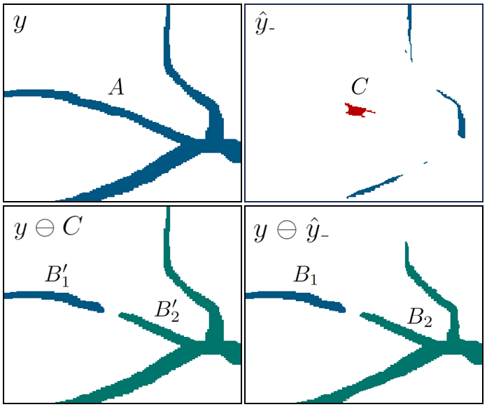
Figure 8: Visualization of Corollary 1.

Computation

Corollary 3.

A component $C\in\mathcal{S}_{y}(\hat{y})$ is negatively critical with $|\mathcal{S}(y)|\neq|\mathcal{S}(y\ominus C)|$ if and only if $\exists A\in\mathcal{S}(y)$ with $A\supseteq C$ such that either $(1)$ $\nexists\,i\in D(C)$ with $i\in A$ or $(2)$ $\exists B_{1},B_{2}\in\mathcal{S}(y\ominus\hat{y})$ with $B_{1},B_{2}\subset A$ such that $i\in B_{1}$ and $j\in B_{2}$ for some $i,j\in D(C)$.

Proof.

First, we prove that Condition 1 is equivalent to Condition 1 in Corollary 1. For the forward direction, Lemma 2 implies that $C\subseteq A$. Now choose any $i\in A$, then it must be the case that $i\in C$ since $A$ is connected and $\nexists j\in D(C)$ with $y_{i}=y_{j}$. The converse is trivial since $A=C$ implies that

$$D(C)=N(C)\setminus C=N(A)\setminus A$$

and so $\nexists i\in D(C)$ with $i\in A$ since the set $A$ is entirely removed from $D(c)$.

Next, we prove that Condition 2 is equivalent to Condition 2 in Corollary 1. Let $v_{0}=i$ and $v_{k}=j$, there exists a path connecting these vertices contained in $C$ since these nodes are connected to the boundary of $C$ which is a connected set. For the converse, $B_{1}\cup C\cup B_{2}$ being connected but $B_{1}\cup B_{2}$ being disconnected implies that there exists a path $(v_{0},\ldots,v_{k})$ from $B_{1}$ to $B_{2}$ via $C$. Since this path passes through $C$, it must be the case that $\exists v_{i},v_{j}\in D(C)$ such that $v_{i}\in B_{1}$ and $v_{j}\in B_{2}$. ∎

Theorem 2.

The computational complexity of computing critical components is $\mathcal{O}(n)$ with respect to the number of voxels in the image.

Proof.

This algorithm involves first precomputing the false negative and false positive masks which can be computed in linear time by comparing each entry in the prediction and ground truth. Next, we must also precompute the following sets of connected components: $\mathcal{S}(y)$, $\mathcal{S}(\hat{y})$, $\mathcal{S}(y\ominus\hat{y})$, and $\mathcal{S}(\hat{y}\ominus\hat{y}_{+})$. Since connected components can be computed in linear time, these precomputations can also be done in linear time (Cormen et al. 2009).

Next, a BFS is performed over both $\hat{y}$ and $\hat{y}_{+}$ to extract the connected components of the false negative and/or positive masks. During this BFS, we can determine whether a component satisfies Corollary 3 in lines 14-21 in Algorithm 2. A BFS is a linear time algorithm (Cormen et al. 2009). Since the operations in lines 13-18 can be achieved in constant time, the complexity of this BFS is still linear. ∎

Algorithm 1 Detection of Critical Components

1:procedure detect criticals($y,\;\hat{y}$):

2:  $\hat{y}\leftarrow$ compute false negatives

3:  $\mathcal{S}(y)\leftarrow$ compute connected components

4:  $\mathcal{S}(y\ominus\hat{y})\leftarrow$ compute connected components

5:  $\mathcal{N}(\hat{y})=$ get critical($y,\;\hat{y},\;\mathcal{S}(y),\;\mathcal{S}(y\ominus\hat{y})$)

6:  

7:  $\hat{y}_{+}\leftarrow$ compute false positives

8:  $\mathcal{S}(\hat{y})\leftarrow$ compute connected components

9:  $\mathcal{S}(\hat{y}\ominus\hat{y}_{+})\leftarrow$ compute connected components

10:  $\mathcal{P}(\hat{y}_{+})=$ get critical($\hat{y},\;\hat{y}_{+},\;\mathcal{S}(\hat{y}),\;\mathcal{S}(\hat{y}\ominus\hat{y}_{+})$)

11:  return $\mathcal{N}(\hat{y}),\;\mathcal{P}(\hat{y}_{+})$

12:end procedure

13:

14:# Note that $\hat{y}_{\times}$ is a placeholder for $\hat{y}$ and $\hat{y}_{+}$

15:procedure get critical($y,\;\hat{y}_{\times},\;\mathcal{S}(y),\;\mathcal{S}(y\ominus\hat{y}_{\times})$)

16:  $F(\hat{y}_{\times})\leftarrow$ compute foreground

17:  $\mathcal{X}(\hat{y}_{\times})=\text{set}()$

18:  while $|F(\hat{y}_{\times})|>0:$

19:      $r=$ sample($F(\hat{y}_{\times})$)

20:      $C,\;is\rule[-0.86108pt]{5.69054pt}{0.4pt}critical=$ get component($y,\;\hat{y}_{\times},\;\mathcal{S}(y),\;\mathcal{S}(y\ominus\hat{y}_{\times}),\;r$)

21:      $F(\hat{y}_{\times}$).remove($C$)

22:      if $is\rule[-0.86108pt]{5.69054pt}{0.4pt}critical:$

23:       $\mathcal{X}(\hat{y}_{\times})$.add($C$)

24:  return $\mathcal{X}(\hat{y}_{\times})$

25:end procedure

Algorithm 2 Check if Component is Critical

1:procedure get component($y,\;\hat{y}_{\times},\;\mathcal{S}(y),\;\mathcal{S}(y\ominus\hat{y}_{\times}),\;r$ ):

2:  $C=\text{set}()$

3:  $collisions=\text{dict}()$

4:  $is\rule[-0.86108pt]{5.69054pt}{0.4pt}critical=$ False

5:  $queue=[r]$

6:  while $|queue|>0:$

7:      $i=queue.\text{pop}()$

8:      $C.\text{add}(i)$

9:      for $j$ in $N(i)$:

10:       if $y_{j}==y_{r}$:

11:        if $(\hat{y}_{\times})_{j}==1$:

12:          $queue.\text{push}(j)$

13:        else:

14:          $\ell_{j}=$ get label($\mathcal{S}(y),\,j$)

15:          if $\ell_{j}$ not in $collisions.\text{keys}()$:

16:           $collisions[\ell_{j}]=$ get label($\mathcal{S}(y\ominus\hat{y}_{\times}),\,j$)

17:          elif $collisions[\ell_{j}]\mathrel{\mathtt{!=}}$ get label($\mathcal{S}(y\ominus\hat{y}_{\times}),\,j$):

18:           $is\rule[-0.86108pt]{5.69054pt}{0.4pt}critical$ = True

19:  if $y_{r}$ not in $collisions.\text{keys}()$ :

20:      $is\rule[-0.86108pt]{5.69054pt}{0.4pt}critical=$ True

21:  return $C,\;is\rule[-0.86108pt]{5.69054pt}{0.4pt}critical$

22:end procedure

Appendix B Extension to Affinity Models

An affinity model is a graph-based segmentation method where the main objective is to predict whether neighboring nodes belong to the same segment. Given a graph $G=(V,E)$ and ground truth segmentation $y$, let $\delta:E\rightarrow\{0,1\}$ be the affinity function given by

$$\delta(\{i,j\})=\begin{cases}1,&\text{if }i,j\in A\\ 0,&\text{otherwise}\end{cases}$$

for some $A\in\mathcal{S}(y)$. One key advantage of affinity models is that they allow instance segmentation to be equivalently formulated as a binary classification task. This formulation is particularly useful when the number of segments is unknown and when distinct objects may be in close contact or even touch.

Neural networks have been used to learn affinities for image segmentation tasks (Turaga et al. 2010). In this approach, the model learns affinity channels, where each channel represents the connectivity between voxels along a certain direction (e.g. vertical or horizontal). The loss function is then computed as a sum over individual losses, each corresponding to one of these affinity channels.

Definition 4.

Let $\mathcal{L}_{k}:\mathbb{R}^{nk}\times\mathbb{R}^{nk}\rightarrow\mathbb{R}$ be the loss function for an affinity model with $k$ channels be given by

$$\mathcal{L}_{k}(y,\hat{y})=\sum_{i=1}^{k}\mathcal{L}(y^{(i)},\hat{y}^{(i)})$$

where $y^{(i)},\hat{y}^{(i)}$ are binary affinities corresponding to the $i$-th channel and $\mathcal{L}$ is the loss function from Definition 1.

Affinity models involve a transformation between voxel- and edge-based representations of an image. Importantly, critical components are defined within the context of a voxel-based representation. Therefore, each affinity prediction must first be transformed into a voxel-based representation, where the critical components are computed. Afterward, these critical components must be converted back into the affinity-based representation to ensure that topological information is properly incorporated into the segmentation process.

Appendix C Experiments

Training Protocol

In experiments involving the EXASPIM dataset, we trained all models using binary cross-entropy to learn three affinity channels representing voxel connectivity along the vertical, horizontal, and depth axes. Each model was trained for a total of 2000 epochs with the learning rate $10^{-3}$ and batch size 8. For the topological loss functions, we used the first 300 epochs to train a U-Net model, then fine-tuned the model for the last 1700 epochs.

The affinity predictions were then processed using a watershed algorithm to agglomerate a 3-d over-segmentation derived from the predicted affinities. This segmentation training and inference pipeline was implemented using the following Github repositories: https://github.com/jgornet/NeuroTorch and https://github.com/funkey/waterz.

Voxel-Based Metrics

Accuracy: Fraction of correctly labeled voxels.

Dice: Metric that combines precision and recall into a single value to provide a balanced measure of a model’s performance.

Adjusted Rand Index (ARI): Measures the similarity between two clusterings by comparing the agreement and disagreement in pairwise assignments. In this version of the Rand index, a value of zero is excluded, ensuring a more refined comparison of clustering performance (Rand 1971).

Variation of Information (VOI): Distance measure between two clusterings that quantifies the amount of information lost or gained when transitioning between clusterings (Meilă 2003).

Skeleton-Based Metrics

Let $G_{i}=(V_{i},E_{i})$ be an undirected graph representing the skeleton of the $i$-th object in a ground truth segmentation $y$. Let $\{S_{1},\ldots,S_{n}\}$ denote a collection of such skeletons such that there is a bijection between skeletons and objects in the ground truth segmentation. Each node $u\in V_{i}$ has a 3-d coordinate $\varphi(u)$ that represents some voxel in $y$. Let $\hat{y}$ be the predicted segmentation to be evaluated. Finally, let $\hat{y}[\varphi(u)]$ be the label of voxel $u$ in the predicted segmentation.

The core idea behind skeleton-based metrics is to evaluate the accuracy of a predicted segmentation by comparing it to a set of ground truth skeletons. A key challenge in this process is to ensure that these metrics are robust to minor misalignments between the segmentation and skeletons (e.g., see Node 4 in Figure 9). To address this, a preprocessing step performs a depth-first search to identify pairs of vertices $u,v\in V_{i}$ that satisfy the following conditions:

• $\hat{y}[\varphi(u)]=\hat{y}[\varphi(v)]$ and $\hat{y}[\varphi(u)]\neq 0$

• There exists a path $\{u,w_{1},\ldots,w_{t},v\}\subseteq V_{i}$ such that $\hat{y}[\varphi(w_{j})]=0$ for $j=1,\ldots,t$.

For any pair of vertices $u,v\in V_{i}$ that satisfy these conditions, we update the predicted segmentation along the detected path by setting $\hat{y}[\varphi(w_{j})]:=\hat{y}[\varphi(u)]$ for $j=1,\ldots,t$.

Let $G_{i}[U_{i}]$ be the subgraph induced by the vertex subset given by $U_{i}=\{u\in V_{i}:\hat{y}[\varphi(u)]\neq 0\}$. Using this definition, we define the following metric

$$\textbf{Splits / Neuron}=\sum\limits_{i=1}^{n}w_{i}\big{(}\big{|}\mathcal{S}(G[U_{i}])\big{|}-1\big{)},$$

where $w_{j}=|E_{j}|\;/\;\sum\limits_{i=1}^{n}|E_{i}|$. Intuitively, this metric computes a weighted average of the number of splits per skeleton.

An edge $\{u,v\}\in E_{i}$ is said to be omit if either $\hat{y}[\varphi(u)]=0$ or $\hat{y}[\varphi(v)]=0$. Using this definition, the metric % Omit is given by

$$\textbf{\% Omit}=100\cdot\frac{\sum\limits_{i=1}^{n}\big{|}\big{\{}\{u,v\}\in E_{i}:\{u,v\}\text{ is omit}\big{\}}\big{|}}{\sum\limits_{i=1}^{n}|E_{i}|}.$$

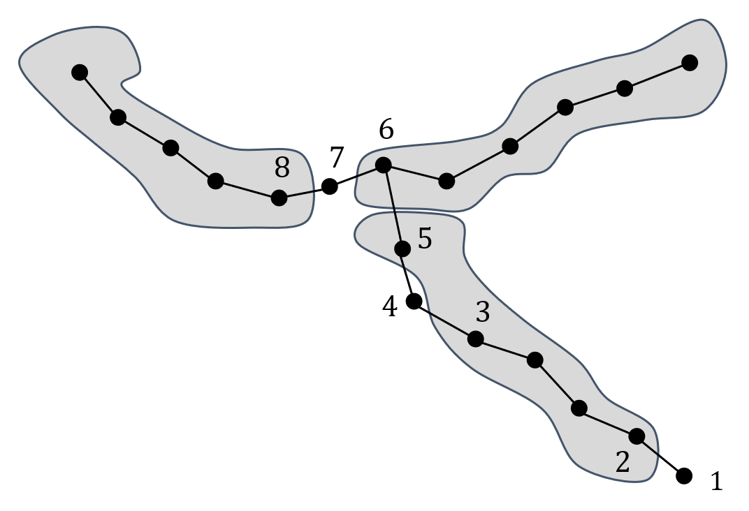
Figure 9: One ground truth skeleton and a predicted segmentation consisting of three connected components. Node 4 is slightly misaligned, its label would be updated to match Nodes 3 and 5. Edge $\{1,2\}$ is omit, but not counted in the metric Splits / Neuron. Edge $\{5,6\}$ is a split and there is a split between nodes 6 and 8. Edges $\{6,7\}$ and $\{7,8\}$ are also omit.

Given the collection of subgraphs $\{G_{1}[U_{1}],\ldots,G_{n}[U_{n}]\}$, two connected components $C_{1}\in\mathcal{S}(G_{i}[U_{i}])$ and $C_{2}\in\mathcal{S}(G_{j}[U_{j}])$ with $i\neq j$ are said to be merged if there exists a pair of nodes $u\in C_{1}$ and $v\in C_{2}$ such that $\hat{y}[\varphi(u)]=\hat{y}[\varphi(v)]$. Let $M_{i}[U_{i}]$ be the set of all such components within the subgraph $G[U_{i}]$. Using this definition, we define the following metric

$$\textbf{\% Merged}=100\cdot\frac{\sum\limits_{i=1}^{n}\sum\limits_{C\in M_{i}[U_{i}]}|C|}{\sum\limits_{i=1}^{n}|E_{i}|}$$

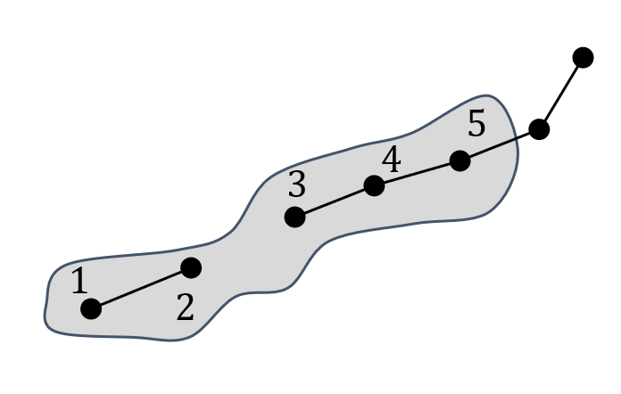
Figure 10: Two ground truth skeleton and a predicted segmentation consisting of one connected component. Edges $\{1,2\}$, $\{3,4\}$, and $\{4,5\}$ are merged.

Using the previous two metrics, Edge Accuracy is defined as

$$\textbf{Edge Accuracy}=100-(\textbf{\% Omit}+\textbf{\% Merged})$$

Intuitively, edge accuracy represents the percentage of edges from ground truth skeleton that were correctly segmented.

Next, we define expected run length (ERL) metrics which quantify the expected length of a segment corresponding to some uniformly sampled skeleton node. Let $A_{i}=E_{i}\setminus(U_{i}\cup M[U_{i}])$ be the set of correctly segmented edges of the skeleton $G_{i}$. Using this definition, we define the following metrics:

$$\textbf{ERL}_{G_{i}} =\sum_{C\in\mathcal{S}(G_{i}[A_{i}])}|C|\cdot\frac{|C|}{|E_{i}|}$$

$$\textbf{Normalized ERL}_{G_{i}} =\frac{\textbf{ERL}_{G_{i}}}{|E_{i}|}$$

Normalized ERL $$=\sum_{i=1}^{n}w_{i}\cdot\textbf{Normalized ERL}_{G_{i}},$$

where $w_{j}=|E_{j}|\;/\;\sum\limits_{i=1}^{n}|E_{i}|$.

Note that code is publicly available at https://github.com/AllenNeuralDynamics/segmentation-skeleton-metrics

Additional Experimental Results

Figures 11 and 12 show the predicted segmentations for the full images, from which the image patches shown in Figures 5 and 6 were sampled.

Table 3: Quantitative results for different models on several datasets. Results for Dive, Mosin., TopoLoss, and DMT are compiled from (Hu et al. 2023). $\mathcal{O}(\cdot)$: complexity of training iterations, $n$: number of pixels/voxels, $k$: number of pooling operations in clDice.

Method	Complexity	Accuracy $\uparrow$	Dice $\uparrow$	ARI $\uparrow$	VOI $\downarrow$	Betti Error $\downarrow$
DRIVE
U-Net	$\mathcal{O}(n)$	0.945$\pm$0.006	0.749$\pm$0.003	0.834$\pm$0.041	1.98$\pm$0.05	3.64$\pm$0.54
DIVE	$\mathcal{O}(n)$	0.955$\pm$0.002	0.754$\pm$0.001	0.841$\pm$0.026	1.94$\pm$0.13	3.28$\pm$0.64
Mosin.	$\mathcal{O}(n)$	0.954$\pm$0.005	0.722$\pm$0.001	0.887$\pm$0.039	1.17$\pm$0.03	2.78$\pm$0.29
TopoLoss	$\mathcal{O}(n\log n)$	0.952$\pm$0.004	0.762$\pm$0.004	0.902$\pm$0.011	1.08$\pm$0.01	1.08$\pm$0.27
DMT	$\mathcal{O}(n^{2})$	0.955$\pm$0.004	0.773$\pm$0.004	0.902$\pm$0.002	0.88$\pm$0.04	0.87$\pm$0.40
Ours	$\mathcal{O}(n)$	0.953$\pm$0.002	0.809$\pm$0.012	0.943$\pm$0.002	0.48$\pm$0.01	0.94$\pm$0.27
ISBI12
U-Net	$\mathcal{O}(n)$	0.968$\pm$0.002	0.970$\pm$0.005	0.934$\pm$0.007	1.37$\pm$0.03	2.79$\pm$0.27
DIVE	$\mathcal{O}(n)$	0.964$\pm$0.004	0.971$\pm$0.003	0.943$\pm$0.009	1.24$\pm$0.03	3.19$\pm$0.31
Mosin.	$\mathcal{O}(n)$	0.953$\pm$0.006	0.972$\pm$0.002	0.931$\pm$0.005	0.98$\pm$0.04	1.24$\pm$0.25
TopoLoss	$\mathcal{O}(n\log n)$	0.963$\pm$0.004	0.976$\pm$0.004	0.944$\pm$0.008	0.78$\pm$0.02	0.43$\pm$0.10
DMT	$\mathcal{O}(n^{2})$	0.959$\pm$0.004	0.980$\pm$0.003	0.953$\pm$0.005	0.67$\pm$0.03	0.39$\pm$0.11
Ours	$\mathcal{O}(n)$	0.971$\pm$0.002	0.983$\pm$0.001	0.934$\pm$0.001	0.74$\pm$0.03	0.48$\pm$0.02
CrackTree
U-Net	$\mathcal{O}(n)$	0.982$\pm$0.010	0.649$\pm$0.003	0.875$\pm$0.042	1.63$\pm$0.10	1.79$\pm$0.30
DIVE	$\mathcal{O}(n)$	0.985$\pm$0.005	0.653$\pm$0.002	0.863$\pm$0.0376	1.57$\pm$0.08	1.58$\pm$0.29
Mosin.	$\mathcal{O}(n)$	0.983$\pm$0.007	0.653$\pm$0.001	0.890$\pm$0.020	1.11$\pm$0.06	1.05$\pm$0.21
TopoLoss	$\mathcal{O}(n\log n)$	0.983$\pm$0.008	0.673$\pm$0.004	0.929$\pm$0.012	0.99$\pm$0.01	0.67$\pm$0.18
DMT	$\mathcal{O}(n^{2})$	0.984$\pm$0.004	0.681$\pm$0.005	0.931$\pm$0.017	0.90$\pm$0.08	0.52$\pm$0.19
Ours	$\mathcal{O}(n)$	0.986$\pm$0.001	0.667$\pm$0.010	0.914$\pm$0.011	0.98$\pm$0.10	0.51$\pm$0.06
EXASPIM
U-Net	$\mathcal{O}(n)$	0.997$\pm$0.010	0.751$\pm$0.047	0.875$\pm$0.082	1.28$\pm$0.46	0.74$\pm$0.03
Gornet	$\mathcal{O}(n^{2})$	0.994$\pm$0.001	0.777$\pm$0.083	0.901$\pm$0.049	0.65$\pm$0.17	0.42$\pm$0.07
clDice	$\mathcal{O}(kn)$	0.998$\pm$0.004	0.785$\pm$0.032	0.923$\pm$0.071	0.66$\pm$0.51	0.36$\pm$0.07
MALIS	$\mathcal{O}(n^{2})$	0.997$\pm$0.001	0.794$\pm$0.052	0.927$\pm$0.042	0.64$\pm$0.27	0.34$\pm$0.08
Ours	$\mathcal{O}(n)$	0.997$\pm$0.001	0.770$\pm$0.058	0.953$\pm$0.038	0.42$\pm$0.21	0.31$\pm$0.06

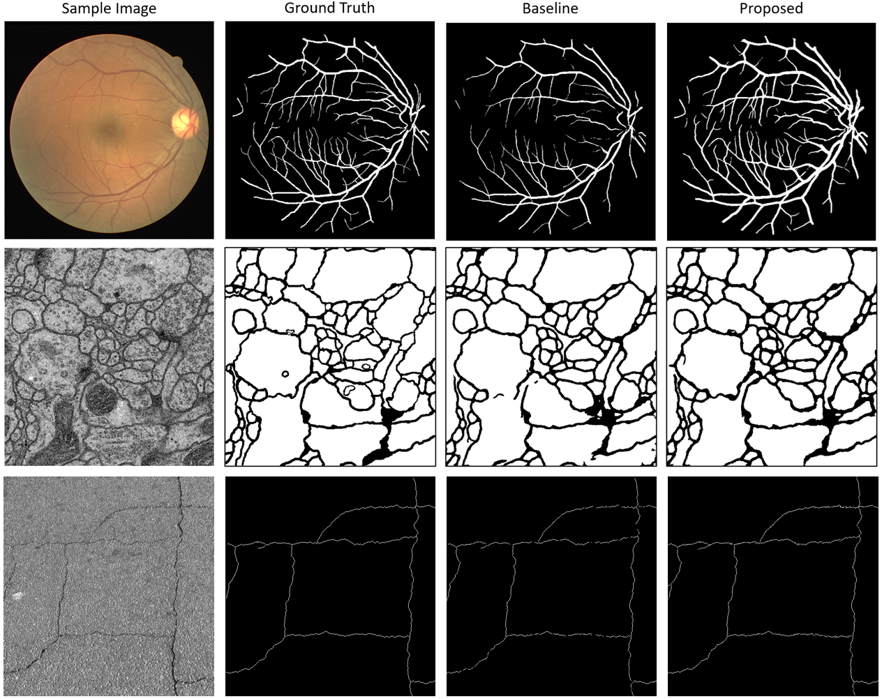
Figure 11: Qualitative results of different models on several 2-d segmentation datasets.

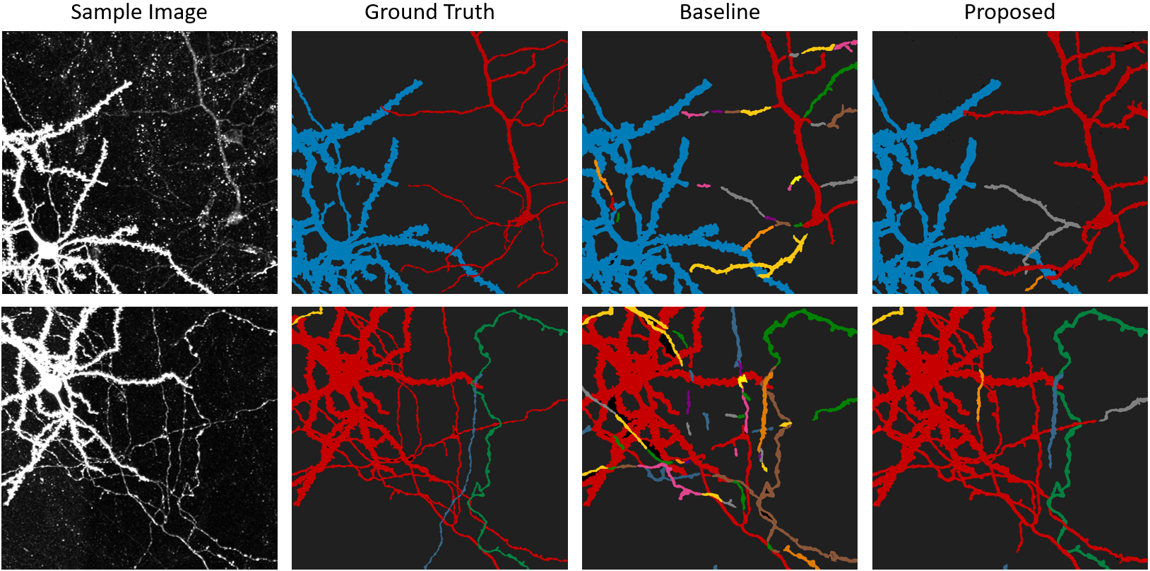
Figure 12: Qualitative results of different models on the 3-d EXASPIM dataset.

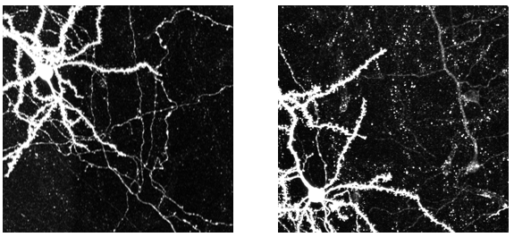
Figure 13: Raw image patches from EXASPIM dataset that the results in Figure 6 were generated from.

Table 4: Average runtimes per epoch for various image patch sizes. Note that runtimes depend on the details of implementation and the hardware.

Method	Complexity	Runtime$/$Epoch $64\times 64\times 64$	Runtime$/$Epoch $128\times 128\times 128$
U-Net	$\mathcal{O}(n)$	2.59$\pm$0.18	10.03$\pm$0.23 sec
Gornet	$\mathcal{O}(n^{2})$	6.88$\pm$0.70	71.62$\pm$1.83 sec
clDice	$\mathcal{O}(kn)$	6.31$\pm$0.71	48.55$\pm$1.60 sec
MALIS	$\mathcal{O}(n^{2})$	5.03$\pm$0.47	50.68$\pm$1.58 sec
Ours	$\mathcal{O}(n)$	7.17$\pm$0.35	20.12$\pm$1.15 sec

References

- Akiba et al. (2019) Akiba, T.; Sano, S.; Yanase, T.; Ohta, T.; and Koyama, M. 2019. Optuna: A Next-generation Hyperparameter Optimization Framework. In Proceedings of the 25th ACM SIGKDD International Conference on Knowledge Discovery and Data Mining.