Scalable Beamforming Design for Multi-RIS-Aided MU-MIMO Systems with Imperfect CSIT

Abstract

A reconfigurable intelligent surface (RIS) has emerged as a promising solution for enhancing the capabilities of wireless communications. This paper presents a scalable beamforming design for maximizing the spectral efficiency (SE) of multi-RIS-aided communications through joint optimization of the precoder and RIS phase shifts in multi-user multiple-input multiple-output (MU-MIMO) systems under imperfect channel state information at the transmitter (CSIT). To address key challenges of the joint optimization problem, we first decompose it into two subproblems with deriving a proper lower bound. We then leverage a generalized power iteration (GPI) approach to identify a superior local optimal precoding solution. We further extend this approach to the RIS design using regularization; we set a RIS regularization function to efficiently handle the unit-modulus constraints, and also find the superior local optimal solution for RIS phase shifts under the GPI-based optimization framework. Subsequently, we propose an alternating optimization method. In particular, utilizing the block-diagonal structure of the matrices the GPI method, the proposed algorithm offers multi-RIS scalable beamforming as well as superior SE performance. Simulations validate the proposed method in terms of both the sum SE performance and the scalability.

I Introduction

A reconfigurable intelligent surface (RIS) has been recognized as a promising technique for future wireless communication systems [1, 2]. By adjusting numerous passive reflecting elements, the RIS enhances wireless channel conditions with flexible control and configuration, resulting in performance improvements with marginal increase in network power consumption. For instance, in millimeter-wave (mmWave) communications, signals can easily experience a severe attenuation due to blockage [3]. To overcome this issue, the deployment of RIS can help creating an additional signal path, thereby increasing the coverage of mmWave systems [4, 5].

Despite the significant potential of the RIS, obtaining precise wireless channel state information (CSI) poses a considerable practical issue in RIS-aided systems [6]. This challenge is exacerbated by the fact that the passive nature of RIS does not facilitate any signal transmission, reception, or processing [7]. In addition, deploying more RISs introduces significant burden on channel estimation, which can lead to substantial performance degradation due to degraded channel estimation accuracy. This challenge motivates to establish beamforming strategies for RIS-aided systems with inaccurate CSI. In this regard, it is imperative to consider robust transmission design that accounts for imperfect CSI at the transmitter (CSIT) and a scalable beamforming strategy to offer a flexible beamforming solution tailored for multi-RIS-aided systems.

I-A Related Works

Because of the promising potential of utilizing the RIS, there exist various analytical works investigating multi-RIS-aided networks. Specifically, wireless networks assisted by two RISs demonstrate that the effective channel benefits from the superposition of the double-reflection link [8]. In [9], it was shown that if the double-reflection channel follows a line-of-sight (LoS) path, it can attain a higher order of passive beamforming gain compared to individual single-reflection links. The outage probability and average symbol error probability for Nakagami-$m$ fading of multi-RIS-aided systems were derived in [10]. The result in [10] indicates that multi-RIS configurations can significantly enhance diversity order and system performance. In [11], the spectral efficiency (SE) of multi-RIS-aided systems was analyzed with Poisson point processes. It was also confirmed in [12] that deploying more RISs up to an optimal number increases the network sum SE, and the optimal number can increase with proper RIS phase optimization. Overall, the literature emphasizes the potential benefit achieved by deploying multiple RISs.

Motivated by the potential of multi-RIS-aided systems, the RIS beamforming optimization have been actively investigated for multiple-input and multiple-output (MIMO) communication systems. According to [13], the problem of maximizing the weighted sum rate in a system supported by multiple RISs was tackled by jointly optimizing the precoder and RIS phase shifts. In [14], the study extended the application of RIS-aided beamforming to multi-cell networks, advancing the methodology to encompass multi-RIS systems through the aggregation of all relevant channel matrices associated with RISs. For a multiuser MIMO (MU-MIMO) downlink system, a codebook-based beamforming method was proposed to minimize transmit power while satisfying quality-of-service (QoS) constraints [15]. It is often considered that the direct link between the base station (BS) and users is not available. For instance, in [16], the RIS-aided communication system was handled through MIMO transmission by considering an upper limit for the channel capacity of the RIS for the blocked direct link scenario. In [4], the hybrid beamforming design was proposed in the RIS-assisted point-to-point MIMO system without the consideration of the direct link. In addition, the RIS can play a pivotal role in supporting various next-generation wireless communication systems, such as integrated sensing and communication as well as low-Earth orbit satellites [17, 18, 19, 20]. Therefore, a comprehensive beamforming optimization framework is indispensable for a general multi-RIS-aided system to fully leverage these diverse applications and maximize system performance.

Considering the difficulty in channel estimation for the RIS-aided system, robust beamforming approaches have been proposed to compensate for channel estimation inaccuracies [21, 22, 23, 24, 25]. In [21], a robust beamforming design was proposed to minimize transmit power under worst-case rate constraints with imperfect CSIT of cascaded channels. The study found that substantial channel estimation errors can significantly degrade overall system performance, and provided engineering insights for the size of the RIS when dealing with imperfect CSIT. In [23], a joint beamforming optimization was tackled for RIS-aided MU-MIMO systems with imperfect CSI, and this work demonstrated that the optimal placement of RIS tends to be closer to the BS. In [25], it was emphasized that precise channel estimation is crucial in achieving max-min fairness and QoS for multi-group systems, noting that deploying RIS may not yield performance gains and could potentially degrade system performance without accurate CSI.

Although several approaches have been successfully proposed by employing famous optimization frameworks such as manifold optimization and successive convex approximation techniques [14, 26, 27, 28, 29, 23, 30, 31, 32], most approaches have achieved sub-optimal solutions, leaving a room for further performance improvement. In addition, some of the proposed approaches have limited scalability for multiple RISs in terms of the computational complexity. Specifically, in [14, 29], circular complex manifold (CCM)-based algorithm and a majorization-minimization (MM)-based algorithm yield sub-optimal performance due to the inherently non-convex nature of the optimization problems. Moreover, regarding the number of RISs $L$, the high-performing algorithms’ complexity increases in the order of $\mathcal{O}(L^{2})$ or even higher [13, 32, 15]. Therefore, there is a need for more effective and scalable beamforming designs tailored for multi-RIS-aided systems which can surpass existing sub-optimal and high-complexity methods, especially for imperfect CSIT scenarios.

I-B Contributions

We investigate the multi-RIS-aided MU-MIMO downlink systems. We formulate a beamforming optimization problem that jointly optimizes the precoder and RIS phase shifts with imperfect CSIT. Due to the non-convex nature of the problem and the unit-modulus constraints imposed by RISs, finding an optimal solution is infeasible. To resolve these challenges, we propose an effective and scalable beamforming optimization framework. The main contributions are summarized as:

• In the considered system, we assume that the estimated channel and its estimation error covariance matrix are known at the BS. Under this assumption, we adopt the instantaneous SE to fully exploit the available channel knowledge, which is desirable to maximize the performance gain. This instantaneous SE is the short-term SE expression that averages channel estimation error distribution. To make this metric tractable, we derive a lower bound of the instantaneous SE. Consequently, our metric involves the channel error covariance as well as the estimated channel, allowing us to exploit the partial CSIT. Based on this approach, we can achieve a robust solution aiming at maximizing the sum SE under imperfect CSIT.

• Using on the derived instantaneous SE bound, we first optimize the precoder based on the generalized power iteration (GPI) method [33]. To this end, we begin with decomposing the problem into two subproblems: $(i)$ the precoder optimization and $(ii)$ the RIS phase shifts optimization. Subsequently, deriving the first-order optimality condition for the precoder with given RIS phase shifts, we interpret the precoding optimization problem as a generalized eigenvalue problem. Subsequently, applying the GPI method, we find the superior local optimal precoding solution that is a principal eigenvector.

• Regarding RIS phase shifts, we develop a regularized GPI method to effectively resolve the unit-modulus constraint and achieve multi-RIS scalability by utilizing a block diagonal structure in the GPI method. Introducing a regularization term as a function of RIS phase shifts, the unit-modulus condition is controlled by the regularization function without the explicit constraint. Through smooth approximation and GPI-friendly reformulation of the problem, we apply the GPI method, ultimately achieving superior local optimal solution.

• Precoding and RIS phase shifts are optimized in an alternating manner under the regularized GPI framework. In particular, utilizing the block-diagonal matrices of the GPI framework, the overall algorithm complexity becomes lower compared to the state-of-the-art beamforming methods and scales linearly with the number of RISs $\mathcal{O}(L)$. For the fixed total number of RIS elements, the complexity scales with respect to $L$ as $\mathcal{O}(1/L^{2})$.

• Via simulations, we demonstrate that our proposed method outperforms baselines across various scenarios, achieving superior local solutions. We also empirically confirm that the regularized GPI approach nearly satisfies the unit-modulus constraint, which verifies the effectiveness of our regularized GPI approach. In addition, we show that our method exhibits its multi-RIS scalability while achieving the highest sum SE.

Notation: The superscripts $(\cdot)^{\sf T}$, $(\cdot)^{\sf H}$, $(\cdot)^{*}$, and $(\cdot)^{-1}$ denote the transpose, Hermitian, complex conjugate, and matrix inversion, respectively. ${\bf{I}}_{N}$ is the identity matrix of size $N\times N$ and $\bf 0$ is a zero vector with proper dimension. We use ${\rm diag}({\bf a})$ for a diagonal matrix with ${\bf a}$ on its diagonal elements. Assuming that ${\bf{A}}_{1},\dots,{\bf{A}}_{N}\in\mathbb{C}^{K\times K}$, ${\bf{A}}={\rm blkdiag}\left({\bf{A}}_{1},\dots,{\bf{A}}_{N}\right)\in\mbox{$\mathbb{C}$}^{KN\times KN}$ is a block diagonal matrix. $\|\bf A\|$ represents L2 norm. We use ${\rm{tr}}(\cdot)$ for trace operator, ${\rm{vec}}(\cdot)$ for vectorization, and $\otimes$ for Kronecker product. With mean $m$ and variance $\sigma^{2}$, we use $\mbox{$\mathcal{C}$}\mbox{$\mathcal{N}$}(m,\sigma^{2})$ for a circularly symmetric complex Gaussian distribution and $\mbox{$\mathcal{N}$}(m,\sigma^{2})$ for a Gaussian distribution.

II System Model And Problem Formulation

II-A Signal Model

As shown in Fig. 1, we consider a multi-RIS-aided MU-MIMO downlink system where the BS equipped with $N$ antennas serves $K$ single-antenna users assisted with $L$ RISs. Each RIS is equipped with $M$ reflecting elements. We denote the user set, RIS set, and RIS phase shifts set as $\mathcal{K}=\left\{1,\cdots,K\right\}$, $\mathcal{L}=\left\{1,\cdots,L\right\}$, and $\mathcal{M}=\left\{1,\cdots,M\right\}$, respectively. The BS determines the optimal phase shifts and conveys the information back to the corresponding RIS controller. The BS broadcasts the data symbols $s_{k}\sim\mbox{$\mathcal{C}$}\mbox{$\mathcal{N}$}(0,P)$, $\forall k\in\mathcal{K}$ to each legitimate user via a precoder ${\bf F}=[{\bf f}_{1},\ldots,{\bf f}_{K}]\in\mbox{$\mathbb{C}$}^{N\times K}$ where ${\bf f}_{k}\in\mbox{$\mathbb{C}$}^{N}$ indicates a precoding vector for $s_{k}$. Then, a transmitted signal vector ${{\bf x}}\in\mbox{$\mathbb{C}$}^{N}$ is given by

$${\bf{x}}=\sum_{k=1}^{K}{\bf{f}}_{k}s_{k}={{\bf F}{\bf s}},$$ (1)

where ${\bf s}=[s_{1},\dots,s_{K}]^{\sf T}\in\mbox{$\mathbb{C}$}^{K}$.

Let ${{\bf H}}_{1,\ell}\in\mathbb{C}^{N\times M}$ and ${{\bf H}}_{2,\ell}\in\mathbb{C}^{M\times K}$ denote an $\ell$th BS-RIS channel matrix and a $\ell$th RIS-user channel matrix, respectively. For the link between RIS $\ell$ and user $k$, we consider ${\bf h}_{2,k,\ell}\in\mbox{$\mathbb{C}$}^{N}$ based on a user channel matrix ${{\bf H}}_{2,\ell}=[{\bf h}_{2,1,\ell},\cdots,{\bf h}_{2,K,\ell}]$. We assume that the direct link between transmitter and receiver is not available. The systems assisted by multiple RISs often ignore secondary reflections between the surfaces, which is a reasonable oversight when the RISs are in each other’s far-field. Thus, we assume a far-field propagation model so that the double-reflection link can be ignored [29]. Accordingly, a received signal at user $k$ is given by

$$y_{k}\!=\!\left(\!\sum_{\ell=1}^{L}{\bf H}_{1,\ell}{\boldsymbol{\Phi}}_{\ell}{\bf h}_{2,k,\ell}\!\right)^{\sf H}\!\!\!{\bf{f}}_{k}s_{k}\!+\!\!\!\sum_{i=1,i\neq k}^{K}\!\!\left(\!\sum_{\ell=1}^{L}{\bf H}_{1,\ell}{\boldsymbol{\Phi}}_{\ell}{\bf h}_{2,k,\ell}\!\right)^{\sf H}\!\!\!{\bf{f}}_{i}s_{i}\!+\!n_{k},$$ (2)

where $n_{k}\sim\mathcal{CN}(0,\sigma^{2})$ is additive white Gaussian noise (AWGN) of the $k$th user.

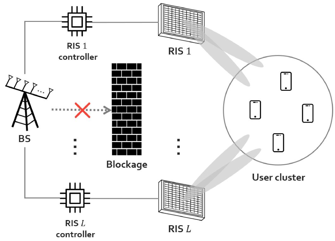
Figure 1: The considered multi-RIS-aided MU-MIMO communication system where the direct link is blocked.

Now, let us define the effective channel matrix between the BS and the $K$ users as

$${\bf H}=\sum_{\ell=1}^{L}{\bf H}_{1,\ell}{\boldsymbol{\Phi}}_{\ell}{\bf H}_{2,\ell}=[{\bf h}_{1},\dots,{\bf h}_{K}].$$ (3)

Then denoting the cascaded channel for user $k$ at RIS $\ell$ as ${\bf H}^{\sf r}_{k,\ell}={\bf H}_{1,\ell}{\rm diag}({\bf h}_{2,k,\ell})\in\mbox{$\mathbb{C}$}^{N\times M}$, we rewrite the effective channel vector of user $k$ as

$${\bf h}_{k}=\sum_{\ell=1}^{L}{\bf H}_{1,\ell}{\boldsymbol{\Phi}}_{\ell}{\bf h}_{2,k,\ell}=\sum_{\ell=1}^{L}{\bf H}_{k,\ell}^{\sf r}{\boldsymbol{\phi}}_{\ell}.$$ (4)

We consider a block fading model where the channel is invariant within each transmission block.

II-B Channel Acquisition Model

We assume that the BS performs uplink channel estimation and thus, the BS only has partial knowledge of the channels due to estimation imperfections. In [34, 29], the RIS channel estimation is implemented for the cascaded channel under a time-division duplex mode. For the cascaded channel, the estimated CSIT is given by

$$\hat{{\bf H}}^{\sf r}_{k,\ell}={\bf H}_{k,\ell}^{\sf r}-{\bf E}_{k,\ell},$$ (5)

or equivalently in a vectorized form, we have

$$\hat{{\bf c}}_{k,\ell}={\bf c}_{k,\ell}-{\bf e}_{k,\ell},$$ (6)

where ${\bf E}_{k,\ell}$ is a channel estimation error matrix, $\hat{{\bf c}}_{k,\ell}={\rm vec}(\hat{{\bf H}}^{\sf r}_{k,\ell})$, ${\bf c}_{k,\ell}={\rm vec}({\bf H}_{k,\ell}^{\sf r})$, and ${\bf e}_{k,\ell}={\rm vec}({\bf E}_{k,\ell})$.

According to [29], using the linear minimum mean square error (LMMSE) estimator with $T_{\sf UL}$ uplink training length, the error covariance matrix is given by

$${\bf R}^{\sf e}_{k,\ell}\!=\!\mbox{$\mathbb{E}$}\left[{\bf e}_{k,\ell}{\bf e}_{k,\ell}^{\sf H}\right]\!=\!\left({\bf C}_{k,\ell}^{-1}+\frac{\rho_{\sf UL}}{\gamma_{k,\ell}\sigma^{2}}{\boldsymbol{\Psi}}_{k,\ell}^{\sf H}{\boldsymbol{\Psi}}_{k,\ell}\otimes{\bf I}_{N}\right)^{-1}\!\!\!\!\!,$$ (7)

where $\rho_{\sf UL}$ is uplink training power, ${\bf C}_{k,\ell}$ is the cascaded channel covariance matrix, ${\boldsymbol{\Psi}}_{k,\ell}$ is the training phase shift matrix of $\ell$th RIS for user $k$, and $\gamma_{k,\ell}$ denotes the pathloss of the cascaded channel determined by $\gamma_{k,\ell}=\gamma_{1,\ell}\gamma_{2,k,\ell}$ where $\gamma_{1,\ell}$ and $\gamma_{2,k,\ell}$ are the pathloss of the $\ell$th RIS-BS and RIS-user $k$, respectively. While the error covariance matrix in (7) remains unaffected by the choice of training signals, the performance of channel estimation is influenced by other factors, particularly the pattern of ${\boldsymbol{\Psi}}_{k,\ell}$. Hence, careful design of an appropriate training matrix ${\boldsymbol{\Psi}}_{k,\ell}$ is crucial for optimizing the channel estimation process. In this paper, we adopt the discrete Fourier transform (DFT)-based training scheme [34]. With the DFT scheme, the error covariance matrix is given by

$${\bf R}^{\sf e}_{k,\ell}=\left({\bf C}_{k,\ell}^{-1}+\frac{T_{\sf UL}\rho_{\sf UL}}{\gamma_{k,\ell}\sigma^{2}}{\bf I}_{NM}\right)^{-1},$$ (8)

where the sequence length for channel training needs to satisfy $T_{\sf UL}\geq MK$. As the uplink training length and power increase to infinity, the error covariance in (8) goes to zero; thereby the CSIT error eventually vanishes.

In the presence of multiple RISs, we assume the on-off scheme for each individual RIS, where each RIS is independently switched on and off [29, 35]. Specifically, the $\ell$th cascaded channel is estimated while turning off all reflecting elements of RISs related to other cascaded channels. Then, each cascaded channel estimation process is divided into $M$ stages in which each stage only estimates one column vector of ${\bf H}^{\sf r}_{k,\ell}$ [36]. Once the channel estimation is completed, all cascaded channels are combined to obtain (4) for all users. We adopt this channel estimation scheme with the LMMSE estimator by taking advantage of leveraging the error covariance matrix in $\eqref{eq:error_cov}$ for our system.

II-C Performance Metrics and Problem Formulation

With the effective channel in (4), the SE of user $k$ is

$$R_{k}=\log_{2}\left(1+\frac{\left|{\bf h}_{k}^{\sf H}{\bf f}_{k}\right|^{2}}{\sum_{i=1,i\neq k}^{K}\left|{\bf h}_{k}^{\sf H}{\bf f}_{i}\right|^{2}+\frac{\sigma^{2}}{P}}\right).$$ (9)

Unfortunately, the BS cannot predict the SE in (9) for perfect CSI. To overcome this, we consider the instantaneous SE defined as $\mbox{$\mathbb{E}$}_{\{{\bf H}_{k,\ell}^{\sf r}|\hat{{\bf H}}^{\sf r}_{k,\ell}\}}\![\!\left.R_{k}\right|\hat{{\bf H}}^{\sf r}_{k,\ell}\!]$ [37, 38]. While an ergodic SE represents the long-term SE achievable when channel coding spans extensive channel blocks, the instantaneous SE refers to the short-term SE expression that averages channel estimation error distribution in each channel realization. We exploit the instantaneous SE to express the ergodic SE in our problem with imperfect CSIT.

According to [37], the ergodic SE of user $k$ is defined as

$$\mbox{$\mathbb{E}$}_{\{{\bf h}_{k}\}}\!\!\left[R_{k}\right] \!=\!\mbox{$\mathbb{E}$}_{\{{{\bf H}}^{\sf r}_{k,\ell},{{\hat{{\bf H}}^{\sf r}_{k,\ell}}}\}}\!\left[R_{k}\right]$$

$$\!=\!\mbox{$\mathbb{E}$}_{{{\{\hat{{\bf H}}^{\sf r}_{k,\ell}}}\!\}}\!\!\left[\mbox{$\mathbb{E}$}_{\{{{\bf H}}^{\sf r}_{k,\ell}\!|{{\hat{{\bf H}}^{\sf r}_{k,\ell}}}\!\}}\!\!\left[R_{k}|\hat{{\bf H}}^{\sf r}_{k,\ell}\right]\!\right]$$ (10)

$$=\!\mbox{$\mathbb{E}$}_{\{{{\hat{{\bf H}}^{\sf r}_{k,\ell}}}\!\}}\!\left[R^{\sf ins}_{k}\right],$$ (11)

where the expectation is taken over the randomness associated with the imperfect knowledge of the channel fading process and $R_{k}^{\sf ins}$ is the instantaneous SE. From (II-C), we define this instantaneous SE as

$$R^{\sf ins}_{k}\!=\!\mbox{$\mathbb{E}$}_{\{{{{{\bf E}}_{k,\ell}}}\}}\!\!\left[\log_{2}\left(1\!+\!\frac{\left|\left(\sum_{\ell=1}^{L}{\bf H}^{\sf r}_{k,\ell}{\boldsymbol{\phi}}_{\ell}\right)^{\sf H}\!\!\!{\bf{f}}_{k}\right|^{2}}{\sum_{i=1,i\neq k}^{K}\!\left|\!\left(\sum_{\ell=1}^{L}\!{\bf H}^{\sf r}_{k,\ell}{\boldsymbol{\phi}}_{\ell}\right)^{\sf H}\!\!\!{\bf{f}}_{i}\right|^{2}\!\!\!+\!\frac{\sigma^{2}}{P}}\right)\right]\!\!.$$ (12)

However, (12) is still not tractable because there exists no closed-form expression for the expectation of the CSIT error. To achieve a closed-form expression for the instantaneous SE, we introduce the following proposition.

Proposition 1.

Using the LMMSE estimator, we consider all channel estimation errors as uncorrelated noise with the transmitted signal. Accordingly, the lower bound of the instantaneous SE is derived as

$$R_{k}^{\sf ins}\! \geq\!\log_{2}\!\left(\!1\!+\!\frac{\left|\left(\sum_{\ell=1}^{L}\hat{{\bf H}}^{\sf r}_{k,\ell}{\boldsymbol{\phi}}_{\ell}\right)^{\sf H}{\bf{f}}_{k}\right|^{2}}{\sum_{i=1,i\neq k}^{K}\!\left|\left(\sum_{\ell=1}^{L}\hat{{\bf H}}^{\sf r}_{k,\ell}{\boldsymbol{\phi}}_{\ell}\right)^{\sf H}\!\!\!{\bf{f}}_{i}\right|^{2}\!\!+\!\sum_{i=1}^{K}{\bf{f}}^{\sf{H}}_{i}{\boldsymbol{\Xi}}_{k}{\bf{f}}_{i}\!+\!\frac{\sigma^{2}}{P}}\!\right)$$

$$=\bar{R}_{k}^{\sf ins}({\bf F},{\boldsymbol{\Phi}}),$$ (13)

where ${\boldsymbol{\Xi}}_{k}=\sum_{\ell=1}^{L}\left({\boldsymbol{\phi}}^{\sf T}_{\ell}\otimes{\bf I}_{N}\right){\bf R}_{k,\ell}^{\sf e}\left({\boldsymbol{\phi}}^{\sf T}_{\ell}\otimes{\bf I}_{N}\right)^{\sf H}$.

Proof.

Using the LMMSE estimator, we can treat channel estimation errors as uncorrelated noise:

$$y_{k}=\left(\sum_{\ell=1}^{L}\hat{{\bf H}}^{\sf r}_{k,\ell}\boldsymbol{\phi}_{\ell}\right)^{\sf H}\!\!\!{\bf{f}}_{k}s_{k}+\sum_{i=1,i\neq k}^{K}\left(\sum_{\ell=1}^{L}\hat{{\bf H}}^{\sf r}_{k,\ell}\boldsymbol{\phi}_{\ell}\right)^{\sf H}\!\!\!{\bf{f}}_{i}s_{i}$$

$$\qquad\qquad\qquad+\underbrace{\sum_{i=1}^{K}\!\left(\sum_{\ell=1}^{L}{{\bf E}}_{k,\ell}\boldsymbol{\phi}_{\ell}\right)^{\sf H}\!\!\!{\bf{f}}_{i}s_{i}}_{{\rm uncorrelated\;errors}}+n_{k}.$$ (14)

Then, the lower bound of the instantaneous SE is derived by the following procedure from (15) to (17) at top of the next page.

$$\mbox{$\mathbb{E}$}_{\{\hat{{\bf H}}^{\sf r}_{k,\ell}\}}\left[R^{\sf ins}_{k}\right] \stackrel{{\scriptstyle(a)}}{{\geq}}\mbox{$\mathbb{E}$}_{\{{{\hat{{\bf H}}^{\sf r}_{k,\ell}}}\}}\left[\log_{2}\left(1\!+\!\frac{\left|\left(\sum_{\ell=1}^{L}\hat{{\bf H}}^{\sf r}_{k,\ell}{\boldsymbol{\phi}}_{\ell}\right)^{\sf H}{\bf{f}}_{k}\right|^{2}}{\sum_{i=1,i\neq k}^{K}\left|\left(\sum_{\ell=1}^{L}\hat{{\bf H}}^{\sf r}_{k,\ell}{\boldsymbol{\phi}}_{\ell}\right)^{\sf H}{\bf{f}}_{i}\right|^{2}+\mbox{$\mathbb{E}$}_{\{{{{{\bf E}}_{k,\ell}}}\}}\left[{\color[rgb]{0,0,0}\sum_{i=1}^{K}{\bf{f}}^{\sf{H}}_{i}\left(\sum_{\ell=1}^{L}{\bf E}_{k,\ell}{\boldsymbol{\phi}}_{\ell}{\boldsymbol{\phi}}_{\ell}^{\sf H}{\bf E}_{k,\ell}^{\sf H}\right){\bf{f}}_{i}}\right]\!+\!\frac{\sigma^{2}}{P}}\right)\right]$$ (15)

$$\stackrel{{\scriptstyle(b)}}{{=}}\mbox{$\mathbb{E}$}_{\{{{\hat{{\bf H}}^{\sf r}_{k,\ell}}}\}}\left[\log_{2}\left(1\!+\!\frac{\left|\left(\sum_{\ell=1}^{L}\hat{{\bf H}}^{\sf r}_{k,\ell}{\boldsymbol{\phi}}_{\ell}\right)^{\sf H}{\bf{f}}_{k}\right|^{2}}{\sum_{i=1,i\neq k}^{K}\left|\left(\sum_{\ell=1}^{L}\hat{{\bf H}}^{\sf r}_{k,\ell}{\boldsymbol{\phi}}_{\ell}\right)^{\sf H}{\bf{f}}_{i}\right|^{2}+{\color[rgb]{0,0,0}\sum_{i=1}^{K}\sum_{\ell=1}^{L}{\bf{f}}^{\sf{H}}_{i}\left({\boldsymbol{\phi}}^{\sf T}_{\ell}\otimes{\bf I}_{N}\right){\bf R}_{k,\ell}^{\sf e}\left({\boldsymbol{\phi}}^{\sf T}_{\ell}\otimes{\bf I}_{N}\right)^{\sf H}{\bf{f}}_{i}}\!+\!\frac{\sigma^{2}}{P}}\right)\right]$$ (16)

$$=\mbox{$\mathbb{E}$}_{\{{{\hat{{\bf H}}^{\sf r}_{k,\ell}}}\}}\left[\bar{R}^{\sf ins}_{k}\right]$$ (17)

 

Specifically, $(a)$ in (15) follows from considering the channel estimation error term as a complex Gaussian distribution and using Jensen’s inequality. For $(b)$ in (16), we apply the vectorization, i.e., ${\rm vec}({\bf A}{\bf B})=({\bf B}^{\sf T}\otimes{\bf I}_{a}){\rm vec}({\bf A})$ with ${\bf A}\in\mbox{$\mathbb{C}$}^{a\times b}$ and ${\bf B}\in\mbox{$\mathbb{C}$}^{b\times c}$, to obtain $\boldsymbol{{{\bf E}}}_{k,\ell}\boldsymbol{\phi}_{\ell}=(\boldsymbol{\phi}_{\ell}^{\sf T}\otimes{\bf I}_{N}){\bf e}_{k,\ell}$. Using this result, we can then calculate the expectation across all channel error terms in the second term of the denominator in (15) as $\mbox{$\mathbb{E}$}\left[\!(\boldsymbol{\phi}_{\ell}^{\sf T}\!\otimes{\bf I}_{N}){\bf e}_{k,\ell}{\bf e}^{\sf H}_{k,\ell}(\boldsymbol{\phi}_{\ell}^{\sf T}\otimes{\bf I}_{N})^{\sf H}\!\right]\!=\!(\boldsymbol{\phi}_{\ell}^{\sf T}\!\otimes{\bf I}_{N}){\bf R}_{k,\ell}^{\sf e}(\boldsymbol{\phi}_{\ell}^{\sf T}\otimes{\bf I}_{N})^{\sf H}\;\forall\ell,k$. This completes the proof. ∎

Thanks to the expression in (13), we are able to leverage the partial channel knowledge, i.e., the channel estimate and its error covariance. Aiming to maximize the sum SE by jointly optimizing the precoder and RIS phase shifts, we formulate the optimization problem with (13) as

$$\mathop{{\text{maximize}}}_{{\bf{f}}_{1},\cdots,{\bf{f}}_{K},{\boldsymbol{\Phi}}} \;\;\sum_{k=1}^{K}\bar{R}^{\sf ins}_{k}({\bf F},{\boldsymbol{\Phi}})$$ (18)

subject to $$\;\;\sum_{k=1}^{K}\left\|{\bf{f}}_{k}\right\|^{2}\leq 1,$$ (19)

$$\;\;|\phi_{\ell,m}|=1,\;\;\forall\ell\in\mathcal{L},\forall m\in\mathcal{M},$$ (20)

where ${\boldsymbol{\Phi}}=[{\boldsymbol{\Phi}}_{1},{\boldsymbol{\Phi}}_{2},\cdots,{\boldsymbol{\Phi}}_{L}]\in\mbox{$\mathbb{C}$}^{M\times LM}$. Since (18) is non-convex, it is challenging to obtain the globally optimal solution. Additionally, the non-convex unit-modulus constraint in (20) further aggravates the challenge. These characteristics render the joint optimization of precoding and RIS phase shifts a highly challenging task. Thus, it is necessary to establish the efficient optimization framework to tackle the problem.

III Proposed Beamforming Design

In this section, we aim to maximize the sum SE by solving the joint optimization problem in (18). To this end, we propose a joint optimization framework that decomposes the problem into two subproblems: $(i)$ the precoder ${\bf F}$ optimization and $(ii)$ the RIS phase shifts $\boldsymbol{\Phi}$ optimization. We then solve these subproblems in an alternating manner under a unified framework to identify a superior local optimal solution.

III-A Optimizing Precoder ${{\bf F}}$

In this subsection, we optimize the precoder ${\bf F}$ while fixing the RIS phase shifts $\boldsymbol{\Phi}$. To highlight this, we omit the notation ${\boldsymbol{\Phi}}$ from ${\bar{R}^{\sf ins}}_{k}({\bf F},{\boldsymbol{\Phi}})$ and thus, we have

$$\mathop{{\text{maximize}}}_{{\bf{f}}_{1},\cdots,{\bf{f}}_{K}} \;\sum_{k=1}^{K}\;{\bar{R}^{\sf ins}}_{k}({\bf F})$$ (21)

subject to $$\;\sum_{k=1}^{K}\left\|{\bf{f}}_{k}\right\|^{2}\leq 1.$$ (22)

Thanks to the reformulation of the original problem with the lower bound of instantaneous SE in (13), we can utilize the GPI approach in [33]. To adopt the method, we first vectorize the precoding matrix as

$$\bar{\mathbf{f}}={\rm{vec}}({\bf F})=\left[\mathbf{f}^{\top}_{1},\mathbf{f}^{\top}_{2},\ldots,\mathbf{f}^{\top}_{K}\right]^{\top}\in\mathbb{C}^{NK}.$$ (23)

Considering the maximum transmit power $P$, we set $\|\bar{\bf f}\|^{2}=1$ to achieve the maximum sum SE. With the estimated cascaded channel of user $k$ denoted as $\hat{{\bf h}}_{k}=\sum_{\ell=1}^{L}\hat{{\bf H}}_{k,\ell}^{\sf r}{\boldsymbol{\phi}}_{\ell}$, we replace $\frac{\sigma^{2}}{P}$ with $\frac{\sigma^{2}}{P}\|{{\bf f}}\|^{2}$ in (13), and rewrite the problem in (21) into more tractable expression, the function of Rayleigh quotient form, as

$$\mathop{{\text{maximize}}}_{\bar{\mathbf{f}}}\sum_{k=1}^{K}\log_{2}\left(\frac{\bar{\mathbf{f}}^{\sf H}\mathbf{A}_{k}\bar{\mathbf{f}}}{\bar{\mathbf{f}}^{\sf H}\mathbf{B}_{k}\bar{\mathbf{f}}}\right),$$ (24)

where

$$\mathbf{A}_{k}=\mathrm{blkdiag}\!\left(\hat{{\bf h}}_{k}\hat{{\bf h}}^{\sf H}_{k}+{\boldsymbol{\Xi}}_{k},\cdots,\hat{{\bf h}}_{k}\hat{{\bf h}}^{\sf H}_{k}+{\boldsymbol{\Xi}}_{k}\right)+\mathbf{I}_{NK}\frac{\sigma^{2}}{P},$$ (25)

$$\mathbf{B}_{k}=\mathbf{A}_{k}-\mathrm{blkdiag}\left(\mathbf{0},\cdots,\hat{{\bf h}}_{k}\hat{{\bf h}}^{\sf H}_{k},\cdots,\mathbf{0}\right).$$ (26)

The second term on the right hand side in (26) has a nonzero block located at the $k$th block entry. We can ignore the transmit power constraint (19) because of $\|\bar{\bf f}\|^{2}=1$ and scaling invariance of $\bar{\bf f}$ in (24). For simplicity, we define the objective function in (24) as

$$\mbox{$\mathcal{L}$}_{\sf BS}(\bar{\bf f})=\log_{2}\prod_{k=1}^{K}\left(\frac{\bar{\mathbf{f}}^{\sf H}\mathbf{A}_{k}\bar{\mathbf{f}}}{\bar{\mathbf{f}}^{\sf H}\mathbf{B}_{k}\bar{\mathbf{f}}}\right)=\log_{2}\lambda_{\sf BS}(\bar{\bf f}).$$ (27)

Then, we derive Lemma 1 to find the stationary points of (27).

Lemma 1.

The stationary condition of the problem (24) is satisfied if the following holds:

$${\bar{{\bf B}}}^{-1}(\bar{\mathbf{f}})\bar{{\bf A}}(\bar{\mathbf{f}})\bar{\mathbf{f}}=\lambda_{\sf BS}(\bar{\mathbf{f}})\bar{\mathbf{f}},$$ (28)

where

$${\bar{{\bf A}}}(\bar{\mathbf{f}})=\lambda_{{\sf BS},{\sf num}}(\bar{\mathbf{f}})\sum_{k=1}^{K}\left(\frac{\mathbf{A}_{k}}{\bar{\mathbf{f}}^{\sf H}\mathbf{A}_{k}\bar{\mathbf{f}}}\right),$$ (29)

$${\bar{{\bf B}}}(\bar{\mathbf{f}})=\lambda_{{\sf BS},{\sf den}}(\bar{\mathbf{f}})\sum_{k=1}^{K}\left(\frac{\mathbf{B}_{k}}{\bar{\mathbf{f}}^{\sf H}\mathbf{B}_{k}\bar{\mathbf{f}}}\right).$$ (30)

and $\lambda_{{\sf BS},{\sf num}}(\bar{\mathbf{f}})$ and $\lambda_{{\sf BS},{\sf den}}(\bar{\mathbf{f}})$ are any functions that meet $\lambda_{{\sf BS}}(\bar{\mathbf{f}})=\lambda_{{\sf BS},{\sf num}}(\bar{\mathbf{f}})/\lambda_{{\sf BS},{\sf den}}(\bar{\mathbf{f}})$.

Proof.

Please refer to Appendix A. ∎

We note that the stationary condition in (28) can be interpreted as a generalized eigenvalue problem. Here, $\lambda_{\sf BS}(\bar{\bf f})$ is as an eigenvalue of ${\bar{{\bf B}}}^{-1}(\bar{\bf{f}})\bar{{\bf A}}(\bar{\bf{f}})$ with $\bar{\bf f}$ as a corresponding eigenvector. As a result, maximizing the objective function $\mbox{$\mathcal{L}$}_{\sf BS}(\bar{\bf f})$ is equivalent to maximizing $\lambda_{\sf BS}(\bar{\bf f})$. Therefore, it is desirable to find the principal eigenvalue of (28) to maximize (27), which is equivalent to finding the superior local optimal solution of (21). Based on (28), we propose the sum SE maximization precoding algorithm by employing the GPI method [33, 39] As described in Algorithm 1, we first initialize $\bar{\bf f}^{(0)}$ and update $\bar{\bf f}^{(t)}$ at each iteration with given $\boldsymbol{\Phi}$; the algorithm computes $\bar{{\bf A}}(\bar{\bf{f}}^{(t-1)})$ and $\bar{{\bf B}}(\bar{\bf{f}}^{(t-1)})$ according to (29) and (30). Then, the algorithm updates $\bar{{\bf f}}_{(t)}$ as

$$\bar{{\bf f}}\leftarrow\bar{{\bf B}}^{-1}(\bar{\bf{f}}^{(t-1)})\bar{{\bf A}}(\bar{\bf{f}}^{(t-1)})\bar{\bf{f}}^{(t-1)}.$$ (31)

The algorithm normalizes the updated precoding vector by $\bar{\bf{f}}^{(t)}=\bar{\bf{f}}^{(t)}/\left\|\bar{\bf{f}}^{(t)}\right\|$. We repeat these steps until either $\bar{\bf{f}}^{(t)}$ converges to a tolerance level (e.g. $\|\bar{{\bf f}}_{(t)}-\bar{{\bf f}}_{(t-1)}\|<\varepsilon_{1}$ for $\varepsilon_{1}>0$) or the algorithm reaches $t_{1,\rm max}$.

1 initialize: ${\bf F}^{(0)}$.

2 Set $\bar{\bf{f}}^{(0)}={\rm vec}({\bf F}^{(0)})$ and $t=1$.

3 while $\left\|\bar{\bf{f}}^{(t)}-\bar{\bf{f}}^{(t-1)}\right\|>\varepsilon_{1}$ or $t\leq t_{1,\max}$ do

4    Build $\bar{{\bf A}}(\bar{\bf{f}}^{(t-1)})$ and $\bar{{\bf B}}(\bar{\bf{f}}^{(t-1)})$ according to (29) and (30) for given $\boldsymbol{\Phi}$.

5    Compute $\bar{\bf{f}}^{(t)}=\bar{{\bf B}}^{-1}(\bar{\bf{f}}^{(t-1)})\bar{{\bf A}}(\bar{\bf{f}}^{(t-1)})\bar{\bf{f}}^{(t-1)}$.

6    Normalize $\bar{\bf{f}}^{(t)}=\bar{\bf{f}}^{(t)}/\left\|\bar{\bf{f}}^{(t)}\right\|$.

7    $t\leftarrow t+1$.

8$\bar{\bf{f}}^{\star}=\left[{\bf{f}}_{1}^{\sf T},{\bf{f}}_{2}^{\sf T},\dots,{\bf{f}}_{K}^{\sf T}\right]^{\sf T}\leftarrow\bar{\bf{f}}^{(t)}$.

return  ${\bf F}^{\star}\leftarrow\bar{\bf{f}}^{\star}$.

Algorithm 1 GPI-Based Precoding Algorithm

III-B Optimizing RIS Phase Shifts ${\boldsymbol{\Phi}}$

In this subsection, we put forth a multi-RIS phase-shifts optimization method for given ${\bf F}$. We have two primary motivations for developing the RIS optimization method within the GPI framework: First, as discussed, the GPI approach offers a significant advantage over traditional optimization methods by enabling us to identify not just any local optimal solution, but a superior local optimum. This capability enhances the overall performance of our RIS system. Second, we aim to achieve efficient scaling with multiple RISs. This is made possible by leveraging the block diagonal structure of matrices within the GPI method, for example, (29) and (30). This structural property, which we will discuss later in Remark 1, allows us to handle multiple RISs without a prohibitive increase in computational complexity.

Unlike the precoding optimization, however, it is required to handle the unit-modulus constraint on ${\boldsymbol{\Phi}}$. To this end, we first reformulate (13) to a quadratic form with respect to $\boldsymbol{\phi}_{\ell}$, providing a more tractable approach in optimizing the RIS phase shifts. Using the vectorization and introducing a permutation matrix, we convert the second term of the denominator in (15) to

$$\sum_{i=1}^{K}{\bf{f}}^{\sf{H}}_{i}\left(\sum_{\ell=1}^{L}{\bf E}_{k,\ell}{\boldsymbol{\phi}}_{\ell}{\boldsymbol{\phi}}_{\ell}^{\sf H}{\bf E}_{k,\ell}^{\sf H}\right){\bf{f}}_{i}$$

$$\!=\!\sum_{\ell=1}^{L}\!\sum_{i=1}^{K}{\boldsymbol{\phi}}_{\ell}^{\sf H}\left({{\bf f}_{i}}^{\sf T}\!\!\otimes{\bf I}_{M}\right)\!{\rm vec}\left({\bf E}^{\sf T}_{k,\ell}\right)^{*}\!\!\left({\rm vec}\left({\bf E}^{\sf T}_{k,\ell}\right)^{*}\right)^{\sf H}\!\!\left({{\bf f}_{i}}^{\sf T}\!\!\otimes{\bf I}_{M}\right)^{\sf H}\!\!\!{\boldsymbol{\phi}}_{\ell}$$

$$\!=\!\sum_{\ell=1}^{L}\!\sum_{i=1}^{K}{\boldsymbol{\phi}}_{\ell}^{\sf H}\left({{\bf f}_{i}}^{\sf T}\otimes{\bf I}_{M}\right)\!{\bf P}{\bf e}_{k,\ell}^{*}\!\left({\bf P}{\bf e}_{k,\ell}^{*}\right)^{\sf H}\!\!\left({{\bf f}_{i}}^{\sf T}\otimes{\bf I}_{M}\right)^{\sf H}\!\!\!{\boldsymbol{\phi}}_{\ell},$$ (32)

where ${\bf P}$ is a permutation matrix satisfying ${\rm vec}({\bf E}^{\sf T})={\bf P}{\rm vec}({\bf E})$. By applying (32) to the similar process of (15)-(17), the lower bound of instantaneous SE can be reformulated as $\tilde{R}^{\sf ins}_{k}({\boldsymbol{\Phi}})=\bar{R}^{\sf ins}_{k}({\bf F},{\boldsymbol{\Phi}})$, where

$$\tilde{R}^{\sf ins}_{k}({\boldsymbol{\Phi}})=$$ (33)

$$\log_{2}\!\left(\!1\!+\!\frac{\left|\left(\sum_{\ell=1}^{L}\hat{{\bf H}}^{\sf r}_{k,\ell}{\boldsymbol{\phi}}_{\ell}\right)^{\sf H}{\bf{f}}_{k}\right|^{2}}{\sum_{i\neq k}^{K}\!\left|\left(\sum_{\ell=1}^{L}\!\hat{{\bf H}}^{\sf r}_{k,\ell}{\boldsymbol{\phi}}_{\ell}\!\right)^{\sf H}\!\!\!{\bf{f}}_{k}\right|^{2}\!\!+\!\sum_{\ell=1}^{L}{\boldsymbol{\phi}}_{\ell}^{\sf H}\boldsymbol{\Theta}_{k,\ell}{\boldsymbol{\phi}}_{\ell}\!+\!\frac{\sigma^{2}}{P}}\!\right),$$

and $\boldsymbol{\Theta}_{k,\ell}=\sum_{i=1}^{K}\left({{\bf f}_{i}}^{\sf T}\otimes{\bf I}_{M}\right){\bf P}\left({\bf R}^{\sf e}_{k,\ell}\right)^{\sf*}{\bf P}^{\sf T}\left({{\bf f}_{i}}^{\sf T}\otimes{\bf I}_{M}\right)^{\sf H}$. With given ${\bf F}$, our problem in (18) is rewritten as

$$\mathop{{\text{maximize}}}_{{\boldsymbol{\Phi}}} \;\;\sum_{k=1}^{K}\tilde{R}^{\sf ins}_{k}({\boldsymbol{\Phi}})$$ (34)

subject to $$\;\;|\phi_{\ell,m}|=1,\;\forall\ell\in\mathcal{L},\forall m\in\mathcal{M}.$$ (35)

Now, to resolve the challenge of the unit-modulus constraint, we introduce a regularization approach. We first stack all individual RIS elements as a vector form as

$$\bar{\boldsymbol{\phi}}\!=\!\left[{\boldsymbol{\phi}}_{1}^{\sf T},\boldsymbol{\phi}_{2}^{\sf T},\cdots,\boldsymbol{\phi}_{L}^{\sf T}\right]^{\sf T}\!\!\!=\!\left[{\phi}_{1,1},{\phi}_{1,2},\cdots,{\phi}_{L,M}\right]^{\sf T}\!\!\in\mbox{$\mathbb{C}$}^{LM}\!\!.$$ (36)

We relax the unit-modulus constraint considering the difference between maximum and minimum values among all RIS phase shifts of $\bar{\boldsymbol{\phi}}$. Then, the regularized optimization problem can be formulated without the unit-modulus constraint as

$$\mathop{{\text{maximize}}}_{{\boldsymbol{\Phi}},\mu} \frac{1}{R_{\Sigma}}\!\sum_{k=1}^{K}\!\tilde{R}^{\sf ins}_{k}({\boldsymbol{\Phi}})\!-\!\frac{\mu}{\tau}\left(\max_{\begin{subarray}{c}\ell\in\mathcal{L}\\ m\in\mathcal{M}\end{subarray}}|{\phi}_{\ell,m}|^{2}\!-\!\min_{\begin{subarray}{c}\ell\in\mathcal{L}\\ m\in\mathcal{M}\end{subarray}}|{\phi}_{\ell,m}|^{2}\right),\!\!$$ (37)

where $\mu$ denotes a parameter of regularization, $\tau$ is a pre-defined normalization factor for the RIS phase shifts, and $R_{\Sigma}$ is a pre-defined normalization factor for the sum SE obtained by any existing state-of-the-art precoder with randomly generated $\boldsymbol{\Phi}$. We remark that the normalization factors are introduced to make the SE and regularization term comparable in scale, thereby reducing the effective range of $\mu$. In (37), the second term, commonly referred to as the penalty term, serves to enforce the unit-modulus constraint by minimizing the difference between maximum and minimum elements of $\bar{\boldsymbol{\phi}}$. The regularization parameter $\mu$ controls the degree of adherence to the unit-modulus constraint, ensuring that the amplitudes of relaxed RIS phase shifts remain as homogeneous as possible before projecting them into a feasible solution set, i.e., a complex unit circle.

We now tackle (37) with respect to ${\bf w}$ for given $\mu$. To transform (37) into a more tractable form, we first normalize the RIS phase shifts vector as

$${{\bf w}}=\frac{1}{\sqrt{LM}}\bar{\boldsymbol{\phi}}=[w_{1},w_{2},\cdots,w_{LM}]^{\sf T}\in\mbox{$\mathbb{C}$}^{LM}.$$ (38)

With some abuse of notation, we then rewrite the objective function in (37) as

$$\mathcal{L}_{\sf RIS}({\bf w})\!=\!\frac{1}{R_{\Sigma}}\!\sum_{k=1}^{K}\!\tilde{R}^{\sf ins}_{k}({\bf w})\!-\!\frac{\mu}{\tau}\left(\max_{i=1,\ldots,LM}\!|w_{i}|^{2}\!-\!\min_{i=1,\ldots,LM}\!|w_{i}|^{2}\right)\!.$$ (39)

We set $\tau=(LM)^{-1}$ in this problem. Let us now introduce a $LM\times LM$ diagonal matrix as

$${\bf X}_{i}={\rm diag}(0,\ldots,\underbrace{1}_{i{\rm th\;term}},\ldots,0),\;i=1,\ldots,LM.$$ (40)

By leveraging (40), we can rewrite the power of the normalized RIS phase shifts as a quadratic form as $|w_{i}|^{2}={\bf w}^{\sf H}{\bf X}_{i}{\bf w}$. To transform (39) into the GPI-friendly form for ${\bf w}$, we assume $\|{\bf w}\|=1$ which is naturally true when the unit-modulus constraint is met. As a result, we can reformulate the objective function in (37) as

$$\mathcal{L}_{\sf RIS} ({\bf w})=\frac{1}{R_{\Sigma}}\sum_{k=1}^{K}\log_{2}\left(\frac{{{\bf w}}^{\sf H}{\bf C}_{k}{{\bf w}}}{{{\bf w}}^{\sf H}{\bf D}_{k}{{\bf w}}}\right)$$

$$-\frac{\mu}{\tau}\left(\max_{i=1,\ldots,LM}\left\{{{\bf w}}^{\sf H}{\bf X}_{i}{{\bf w}}\right\}-\min_{i=1,\ldots,LM}\left\{{{\bf w}}^{\sf H}{\bf X}_{i}{{\bf w}}\right\}\right),$$ (41)

where

$$\mathbf{C}_{k}=\mathrm{blkdiag}\!\left(\Upsilon_{k,1}+\boldsymbol{\Theta}_{k,1},\cdots,\Upsilon_{k,L}+\boldsymbol{\Theta}_{k,L}\right)+\frac{\sigma^{2}}{P}{\bf I}_{LM},$$ (42)

$$\mathbf{D}_{k}=\mathrm{blkdiag}\!\left(\bar{\Upsilon}_{k,1}+\boldsymbol{\Theta}_{k,1},\cdots,\bar{\Upsilon}_{k,L}+\boldsymbol{\Theta}_{k,L}\right)+\frac{\sigma^{2}}{P}{\bf I}_{LM},$$ (43)

$$\Upsilon_{k,\ell}=LM{\hat{{\bf H}}_{k,1}^{\sf rH}}{\bf Q}\hat{{\bf H}}^{\sf r}_{k,\ell},\;\bar{\Upsilon}_{k,\ell}=LM{\hat{{\bf H}}_{k,1}^{\sf rH}}\bar{{\bf Q}}\hat{{\bf H}}^{\sf r}_{k,\ell},$$ (44)

$${\bf Q}=\sum_{i=1}^{K}{\bf f}_{i}{\bf f}_{i}^{\sf H},\;\bar{{\bf Q}}_{k}={\bf Q}-{\bf f}_{k}{\bf f}_{k}^{\sf H}.$$ (45)

In (III-B), we need to approximate the non-smooth functions such as $\rm{max}(\cdot)$ and $\rm{min}(\cdot)$ for finding the optimality condition. To this end, we adopt a LogSumExp approach [40]:

$$\min_{i=1,...,J}\{x_{i}\}\approx-\alpha\ln\left(\sum_{i=1}^{J}\exp\left(\frac{x_{i}}{-\alpha}\right)\right),$$ (46)

$$\max_{i=1,...,J}\{x_{i}\}\approx\frac{1}{\alpha}\ln\left(\sum_{i=1}^{J}\exp\left(\alpha x_{i}\right)\right),$$ (47)

where the approximation becomes tight as $\alpha\rightarrow+0$ for both cases. Using the LogSumExp, (III-B) is approximated as

$$\mathcal{L}_{\sf RIS}({{\bf w}})\approx\tilde{\mathcal{L}}_{\sf RIS}({{\bf w}})=\log_{2}\lambda_{\sf RIS}({\bf w}),$$ (48)

where

$$\lambda_{\sf RIS}({\bf w})\!=\!\prod_{k=1}^{K}\left(\frac{{{\bf w}}^{\sf H}{\bf C}_{k}{{\bf w}}}{{{\bf w}}^{\sf H}{\bf D}_{k}{{\bf w}}}\right)^{\frac{1}{R_{\Sigma}}}\!\left(\sum_{i=1}^{LM}\exp\left(\alpha_{1}{{\bf w}}^{\sf H}{\bf X}_{i}{{\bf w}}\right)\right)^{-\frac{\mu\ln 2}{\tau\alpha_{1}}}$$

$$\qquad\qquad\times\left(\sum_{i=1}^{LM}\exp\left({\frac{{{\bf w}}^{\sf H}{\bf X}_{i}{{\bf w}}}{-\alpha_{2}}}\right)\right)^{-\frac{\alpha_{2}\mu\ln 2}{\tau}}.$$ (49)

Finally, the regularized optimization problem in (37) is reformulated and approximated for given $\mu$ as

$$\mathop{{\text{maximize}}}_{{\bf w}} \;\tilde{\mbox{$\mathcal{L}$}}_{\sf RIS}({{\bf w}}).$$ (50)

Then, similar to the precoding optimization, we derive Lemma 2 for the approximated problem in (50) to find the stationary points of (49).

Lemma 2.

The stationary condition of (50) is also satisfied if the following holds:

$$\bar{{\bf D}}^{-1}({\bf w})\bar{{\bf C}}({\bf w}){{\bf w}}=\lambda_{\sf RIS}({\bf w}){\bf w},$$ (51)

where

$$\bar{{\bf C}}({\bf w})=\lambda_{{\sf RIS},{\sf num}}({\bf w})\times$$

$$\quad\left[\frac{1}{R_{\Sigma}\ln{2}}\sum_{k=1}^{K}\left(\frac{{\bf C}_{k}}{{{\bf w}}^{\sf H}{\bf C}_{k}{{\bf w}}}\right)+\frac{\mu}{\tau}\frac{\sum_{i=1}^{LM}{{\bf X}}_{i}e^{\frac{{{\bf w}}^{\sf H}{{\bf X}}_{i}{{\bf w}}}{-\alpha_{2}}}}{\sum_{i=1}^{LM}e^{\frac{{{\bf w}}^{\sf H}{{\bf X}}_{i}{{\bf w}}}{-\alpha_{2}}}}\right],$$ (52)

$$\bar{{\bf D}}({\bf w})=\lambda_{{\sf RIS},{\sf den}}({\bf w})\times$$

$$\quad\left[\frac{1}{R_{\Sigma}\ln{2}}\sum_{k=1}^{K}\left(\frac{{\bf D}_{k}}{{{\bf w}}^{\sf H}{\bf D}_{k}{{\bf w}}}\right)+\frac{\mu}{\tau}\frac{\sum_{i=1}^{LM}{{\bf X}}_{i}e^{\alpha_{1}{{\bf w}}^{\sf H}{{\bf X}}_{i}{{\bf w}}}}{\sum_{i=1}^{LM}e^{\alpha_{1}{{\bf w}}^{\sf H}{{\bf X}}_{i}{{\bf w}}}}\right].$$ (53)

Proof.

Please refer to Appendix B. ∎

As discussed in Section III-A, this stationary condition can be interpreted as the generalized eigenvalue problem. Thus, the problem is transformed for finding its principal eigenvector of (51). In this regard, such eigenvector can also be found by using the GPI method to solve (51).

We describe our regularized GPI-based RIS phase-shifts optimization method in Algorithm 2. The algorithm first initializes $\bar{\boldsymbol{\phi}}$. To optimize $\bar{\boldsymbol{\phi}}$ with the GPI method, the algorithm builds $\bar{{\bf C}}({{\bf w}}^{(t-1)})$ and $\bar{{\bf D}}({{\bf w}}^{(t-1)})$ for given ${\bf F}$, $\mu$, $R_{\Sigma}$, and $\tau$. From the stationary condition in (51), the algorithm updates ${{\bf w}}^{(t)}$ by calculating ${{\bf w}}^{(t)}=\bar{{\bf D}}^{-1}({{\bf w}}^{(t-1)})\bar{{\bf C}}({{\bf w}}^{(t-1)}){{\bf w}}^{(t-1)}$ and normalizing ${{\bf w}}^{(t)}={{\bf w}}^{(t)}/\left\|{{\bf w}}^{(t)}\right\|$. We repeat these steps until either ${{\bf w}}$ converges to a tolerance level $\varepsilon_{2}>0$ or $t=t_{2,\rm max}$. Lastly, due to the unit-modulus constraint, the optimized ${\bf w}^{\star}$ is projected onto the feasible solution set by computing $\bar{\boldsymbol{\phi}}=e^{j{\rm arg}({\bf w}^{\star})}$, where ${\rm arg}(\cdot)$ denotes the argument of a complex number.

1 initialize: ${\bar{\boldsymbol{\phi}}}^{(0)}\leftarrow\boldsymbol{\Phi}^{(0)}$.

2 Set ${\bf w}^{(0)}=\frac{1}{\sqrt{LM}}{\bar{\boldsymbol{\phi}}}^{(0)}$ and $t=1$.

3 while $\left\|{{\bf w}}^{(t)}-{{\bf w}}^{(t-1)}\right\|>\varepsilon_{2}$ or $t\leq t_{2,\max}$ do

4    Build $\bar{{\bf C}}({{\bf w}}^{(t-1)}\!)$ and $\bar{{\bf D}}({{\bf w}}^{(t-1)}\!)$ with given ${\bf F}$ and $\mu$.

5    Compute ${{\bf w}}^{(t)}\!=\!\bar{{\bf D}}^{-1}({{\bf w}}^{(t-1)})\bar{{\bf C}}({{\bf w}}^{(t-1)}){{\bf w}}^{(t-1)}$.

6    Normalize ${{\bf w}}^{(t)}={{\bf w}}^{(t)}/\left\|{{\bf w}}^{(t)}\right\|$.

7    $t\leftarrow t+1$.

8 ${\bf w}^{\star}\leftarrow{\bf w}^{(t)}$.

9 ${\bar{\boldsymbol{\phi}}}^{\star}\leftarrow e^{j{{\rm arg}({\bf w}^{\star})}}$.

return  ${{\boldsymbol{\Phi}}}^{\star}\leftarrow\bar{\boldsymbol{\phi}}^{\star}$.

Algorithm 2 Regularized GPI-Based RIS Phase-Shifts Optimization Algorithm

III-C Joint Optimization Algorithm

In this subsection, we propose the alternating algorithm as described in Algorithm 3 for joint optimization of the precoder and RIS phase shifts by putting together the results in Section III-A and III-B. At the beginning of Algorithm 3, the algorithm initializes the precoder and the RIS phase shifts as ${\bf F}^{(0)}$ and $\boldsymbol{\Phi}^{(0)}$ while setting the outer iteration count $i=1$. Then, the algorithm computes $R_{\Sigma}$ for given ${\bf F}^{(0)}$ to normalize the penalty term in (37). Recall that we set $\tau=(LM)^{-1}$ for normalization of the RIS regularization term.

For finding an optimal value of $\mu$, we adopt a line search method. With the line search, the algorithm identifies the optimal value of $\mu$ within the range of $\mu^{(i)}\in[\mu_{\rm min},\mu_{\rm max}]$ with $T_{\mu}$ linearly spaced points and the increasing step $\Delta_{\mu}$, i.e., $\mu_{\rm max}=\mu_{\rm min}+\Delta_{\mu}(T_{\mu}-1)$, which is updated in the outer loop. In the inner loop of the algorithm, the precoder is optimized by Algorithm 1 for given $\boldsymbol{\Phi}$. Subsequently, using Algorithm 2, the RIS phase shifts matrix is optimized with updated ${\bf F}$. We repeat these steps until either it converges or $t=t_{3,\rm max}$ in the alternating manner. For the convergence level, we compare the current solution with the previous solution as $\frac{|f({\bf F}^{(t)},\boldsymbol{\Phi}^{(t)})-f({\bf F}^{(t-1)},\boldsymbol{\Phi}^{(t-1)})|}{f({\bf F}^{(t-1)},\boldsymbol{\Phi}^{(t-1)})}$ where $f({\bf F},{\boldsymbol{\Phi}})$ is the objective function of the original problem in (18). We use this convergence level with a tolerance threshold $\varepsilon_{3}>0$. To identify the optimal value of $\mu$, the algorithm computes $f\left(\tilde{{\bf F}}^{(i)},\tilde{\boldsymbol{\Phi}}^{(i)}\right)$ at $\mu^{(i)}$. Consequently, the algorithm decides ${\boldsymbol{\Phi}}^{\star}$ and ${\bf F}^{\star}$ that maximizes $f\left(\tilde{{\bf F}}^{(i)},\tilde{\boldsymbol{\Phi}}^{(i)}\right)$ for $i=1,\cdots,N_{\mu}$.

1 initialize: ${\bf F}^{(0)},{\boldsymbol{\Phi}}^{(0)}$, and $\mu^{(0)}$

2 Set iteration count for outer loop $i=1$.

3 Compute $\tau=(LM)^{-1}$ and $R_{\Sigma}$ with (${\bf F}^{(0)}$, ${{\boldsymbol{\Phi}}}^{(0)}$).

4 while $i\leq{\color[rgb]{0,0,0}T_{\mu}}$ do

5    Set $\mu^{(i)}\leftarrow\mu^{(i-1)}+\Delta_{\mu}\in[\mu_{\rm min},\mu_{\rm max}]$.

6    Set iteration count for inner loop $t=1$.

7    while $\frac{|f({\bf F}^{(t)}\!,\!\boldsymbol{\Phi}^{(t)})-f({\bf F}^{(t-1)}\!,\!\boldsymbol{\Phi}^{(t-1)}\!)|}{f({\bf F}^{(t-1)},\boldsymbol{\Phi}^{(t-1)}\!)}\!>\!\varepsilon_{3}$ or $t\!\leq\!t_{3,\rm max}$ do

8       ${{\bf F}}^{(t)}\leftarrow\text{Algorithm~\ref{alg:algorithm_1}}\left({\bf F}^{(t-1)};{\boldsymbol{\Phi}}^{(t-1)}\right)$.

9       ${\boldsymbol{\Phi}}^{(t)}\leftarrow\text{Algorithm~\ref{alg:algorithm_2}}\left({\boldsymbol{\Phi}}^{(\!t-1\!)};{\bf F}^{(t)},\mu^{(i)}\right).$

10       $t\leftarrow t+1$.

11   $\tilde{{\bf F}}^{(i)}\leftarrow{\bf F}^{(t)}$ and $\tilde{\boldsymbol{\Phi}}^{(i)}\leftarrow\boldsymbol{\Phi}^{(t)}$.

12    Compute $f\left(\tilde{{\bf F}}^{(i)},\tilde{\boldsymbol{\Phi}}^{(i)}\right)$.

13    Set $i\leftarrow i+1$.

14Select $i^{\star}=\mathop{\rm arg\,max}_{i=1,\cdots,{\color[rgb]{0,0,0}T_{\mu}}}{f\left(\tilde{{\bf F}}^{(i)},\tilde{\boldsymbol{\Phi}}^{(i)}\right)}$.

return  ${\bf F}^{\star}\leftarrow\tilde{{\bf F}}^{(i^{\star})}$ and ${{\boldsymbol{\Phi}}}^{\star}\leftarrow\tilde{\boldsymbol{\Phi}}^{(i^{\star})}$.

Algorithm 3 GPI-Based Precoding and RIS Phase-Shifts Optimization Algorithm (GPI-PRIS)

III-D Complexity Analysis

Now, we analyze the complexity of the proposed algorithms. The complexity of Algorithm 1 is dominated by the inversion in $\bar{{\bf B}}^{-1}(\bar{\bf{f}})$. Since $\bar{{\bf B}}(\bar{\bf{f}})$ is a block-diagonal and symmetry matrix, we need $\mathcal{O}(KN^{3})$ instead of $\mathcal{O}(K^{3}N^{3})$ to obtain the inverse of $K$ sub-matrices in $\bar{{\bf B}}(\bar{\bf{f}})$. Hence, the total complexity of Algorithm 1 is $\mathcal{O}(T_{1}KN^{3})$ where $T_{1}$ is the number of its iterations. We note that this is substantially lower compared to the existing precoding schemes. For instance, the weighted mean square error (WMMSE) method [41] needs the complexity order of $\mathcal{O}((KN)^{3.5})$ based on a quadratically constrained quadratic programming problem.

Similarly, Algorithm 2 complexity is dominated by the inversion in $\bar{{\bf D}}^{-1}({\bf w})$ for the regularized GPI method. Since $\bar{{\bf D}}({\bf w})$ is also a block-diagonal and symmetry matrix, we only need $\mathcal{O}(LM^{3})$ to obtain the inverse of each sub-matrix in $\bar{{\bf D}}({\bf w})$. Accordingly, the total complexity of Algorithm 2 is $\mathcal{O}(T_{2}LM^{3})$ where $T_{2}$ is the number of its iterations. The state-of-the-art RIS phase-shifts optimization scheme such as the MM algorithm or the CCM algorithm have the complexity order of $\mathcal{O}(M^{3}+T_{i}M^{2})$ where $T_{i}$ denotes the number of iterations required for the MM algorithm or the CCM algorithm with $i\in\{\rm{MM,CCM}\}$ in single-RIS-aided systems [14]. Extension to multi-RIS systems, they further need the complexity order of $\mathcal{O}((LM)^{3}+T_{i}(LM)^{2})$ [32].

Finally, let us denote the number of iterations set for the line search of $\mu$ as $T_{\mu}$. Then, the total complexity of Algorithm 3 (GPI-PRIS) is $\mathcal{O}(T_{\mu}(T_{1}KN^{3}+T_{2}LM^{3}))$. Considering $M>N$, the main bottle neck arises from Algorithm 2, and the complexity becomes $\mathcal{O}(T_{\mu}T_{2}LM^{3})$.

Remark 1 (Complexity Comparison and Scalability).

Our algorithm has a comparable complexity order to representative RIS optimization schemes in terms of $M$. However, owing to the special structure of $\bar{{\bf D}}({\bf w})$, a block diagonal and symmetric matrix, our algorithm exhibits linear scaling with respect to $L$. This linear growth makes the algorithm particularly advantageous for scalable beamforming in multi-RIS-aided systems when efficient handling of a large number of RISs is essential. In addition, since it was observed that increasing the number of RISs with fixed total RIS elements $M_{\rm tot}$ (for example, $M=M_{\rm tot}/L$) is advantageous up to a certain optimal $L$ [12], our algorithm provides a particularly more significant RIS scalability for the fixed $M_{\rm tot}$ case whose complexity scales as $\sim M_{\rm tot}^{3}/L^{2}$, allowing for flexible deployment of multiple RISs to maximize the sum SE. This is also numerically verified in Fig. 9 in Section IV-B.

IV Numerical Results

In this section, we evaluate the sum SE and the computational complexity of the proposed algorithm (GPI-PRIS). Baseline state-of-the-art methods for comparison are

• Alg 1-MM: In this method, we use the Algorithm 1-based precoder, and the RIS phase shifts are optimized by the MM algorithm [14].

• WMMSE-MM: In this method, we use the WMMSE-based precoding algorithm [41] solved by CVX, and the RIS phase shifts are optimized by the MM algorithm [14].

• RZF-MM: In this method, we use the regularized zero-forcing (RZF) precoder. The RIS phase shifts are optimized by the MM algorithm [14].

• Alg 1-Random: This case indicates that using Algorithm 1, the phase shift of each RIS element is randomly selected.

• RZF-Random: This case indicates that using RZF, the phase shift of each RIS element is randomly selected.

We use RZF as an initial precoder of Algorithm 1. Using the line search method with $T_{\mu}=30$ linearly spaced points, we identify the optimal value of $\mu$ in range $\mu\in[0,100]$. We set the maximum iteration counts to be $t_{1,{\rm max}}=t_{2,{\rm max}}=t_{3,{\rm max}}=20$, tolerance levels as $\varepsilon_{1}=\varepsilon_{2}=\varepsilon_{3}=0.01$, and $\alpha_{1}=\alpha_{2}=2$. For the MM-based baseline schemes, we consider the same tolerance level and iteration counts as the proposed algorithm.

IV-A Simulation Environments

In the considered system, we assume that a uniform linear array (ULA) at the BS and the RIS reflecting elements are arranged in a uniform planar array (UPA). The small wavelength of mmWave signals restricts their ability to diffract around obstacles. Consequently, mmWave channels typically display a sparse multipath structure and are often modeled using the Saleh-Valenzuela (SV) channel [42]. Applying the SV channel model in the presence of the same spatial paths $L_{\sf BR}$ for all BS-RIS links, the channel matrix between the BS and RIS $\ell$ is given by

$${\bf H}_{1,\ell}=\frac{1}{\sqrt{L_{\sf BR}}}\sum_{i=1}^{L_{\sf BR}}\sqrt{\gamma_{1,\ell}}{\bf a}_{\sf B}(\vartheta^{\sf B}_{i,\ell}){\bf a}_{\sf R}^{\sf H}(\varphi^{a}_{i,\ell},\varphi^{e}_{i,\ell}),$$ (54)

where $\gamma_{1,\ell}$ is the path gain of $\ell$th BS-RIS link, $\vartheta^{\sf B}_{i,\ell}$ denotes angle of departure (AoD), $(\varphi^{e}_{i,\ell},\varphi^{a}_{i,\ell})$ denote the angles of arrival (AoA) which consists of the elevation $\varphi^{e}_{i,\ell}$ and azimuth angles $\varphi^{a}_{i,\ell}$ of $\ell$th RIS, and ${\bf a}(\cdot)$ denotes a steering vector. With a $N$-element ULA, the steering vector at the BS is defined as

$${\bf a}_{\sf B}(\vartheta^{\sf B}_{i,\ell})=\left[1,e^{j2\pi\frac{\Delta_{\sf B}}{\lambda_{c}}\sin\vartheta^{\sf B}_{i,\ell}},\ldots,e^{j2\pi(N-1)\frac{\Delta_{\sf B}}{\lambda_{c}}\sin\vartheta^{\sf B}_{i,\ell}}\right]^{\sf T},$$ (55)

where $\lambda_{c}$ denotes the carrier wavelength, $\Delta_{\sf B}$ denotes the antenna spacing. In addition, the steering vectors of an $M=M_{y}\times M_{z}$ UPA on the $yz$-plane are expressed as

$${\bf a}_{\sf R}(\varphi^{a}_{i,\ell},\varphi^{e}_{i,\ell})={\bf a}_{y}(\varphi^{a}_{i,\ell},\varphi^{e}_{i,\ell})\otimes{\bf a}_{z}(\varphi^{e}_{i,\ell}),$$ (56)

where the array response vectors are defined as

$${\bf a}_{y}(\varphi^{a}_{i,\ell},\varphi^{e}_{i,\ell})$$ (57)

$$\!=\!\left[\!1,e^{j2\pi\frac{\Delta_{y}}{\lambda_{c}}\!\sin(\varphi^{a}_{i,\ell})\!\sin(\varphi^{e}_{i,\ell})},\ldots,e^{j2\pi(M_{y}\!-\!1)\frac{\Delta_{y}}{\lambda_{c}}\!\sin(\varphi^{a}_{i,\ell})\!\sin(\varphi^{e}_{i,\ell})}\!\right]^{\!\sf T}\!\!\!,$$

$${\bf a}_{z}(\varphi^{e}_{i,\ell})\!=\!\left[1,e^{j2\pi\frac{\Delta_{z}}{\lambda_{c}}\!\cos(\varphi^{e}_{i,\ell})},\!\ldots\!,e^{j2\pi(M_{z}-1)\frac{\Delta_{z}}{\lambda_{c}}\!\cos(\varphi^{e}_{i,\ell})}\right]^{\sf T}\!\!\!,$$ (58)

where $\Delta_{y}$ and $\Delta_{z}$ are the distance between adjacent RIS reflecting elements along two axes.

We assume that the same total number of spatial paths between the RIS and user is $L_{\sf RU}$ for all RIS-user links. Based on the SV channel model, the RIS-user channel is

$${\bf h}_{2,k,\ell}=\frac{1}{\sqrt{L_{\sf RU}}}\sum_{i=1}^{L_{\sf RU}}\sqrt{{\gamma}_{2,k,\ell}}\alpha^{\sf sc}_{k,\ell}{\bf a}_{\sf R}(\varphi^{a}_{k,i,\ell},\varphi^{e}_{k,i,\ell}),$$ (59)

where $\gamma_{2,k,\ell}$ denotes the path gain of the RIS-user link, $\alpha^{\sf sc}_{k,\ell}$ denotes small-scale fading satisfying $\alpha^{\sf sc}_{k,\ell}\sim\mbox{$\mathcal{C}$}\mbox{$\mathcal{N}$}(0,1)$ due to user movement, and $(\varphi^{a}_{k,i,\ell},\varphi^{e}_{k,i,\ell})$ denote and azimuth and elevation AoD between user $k$ and RIS $\ell$.

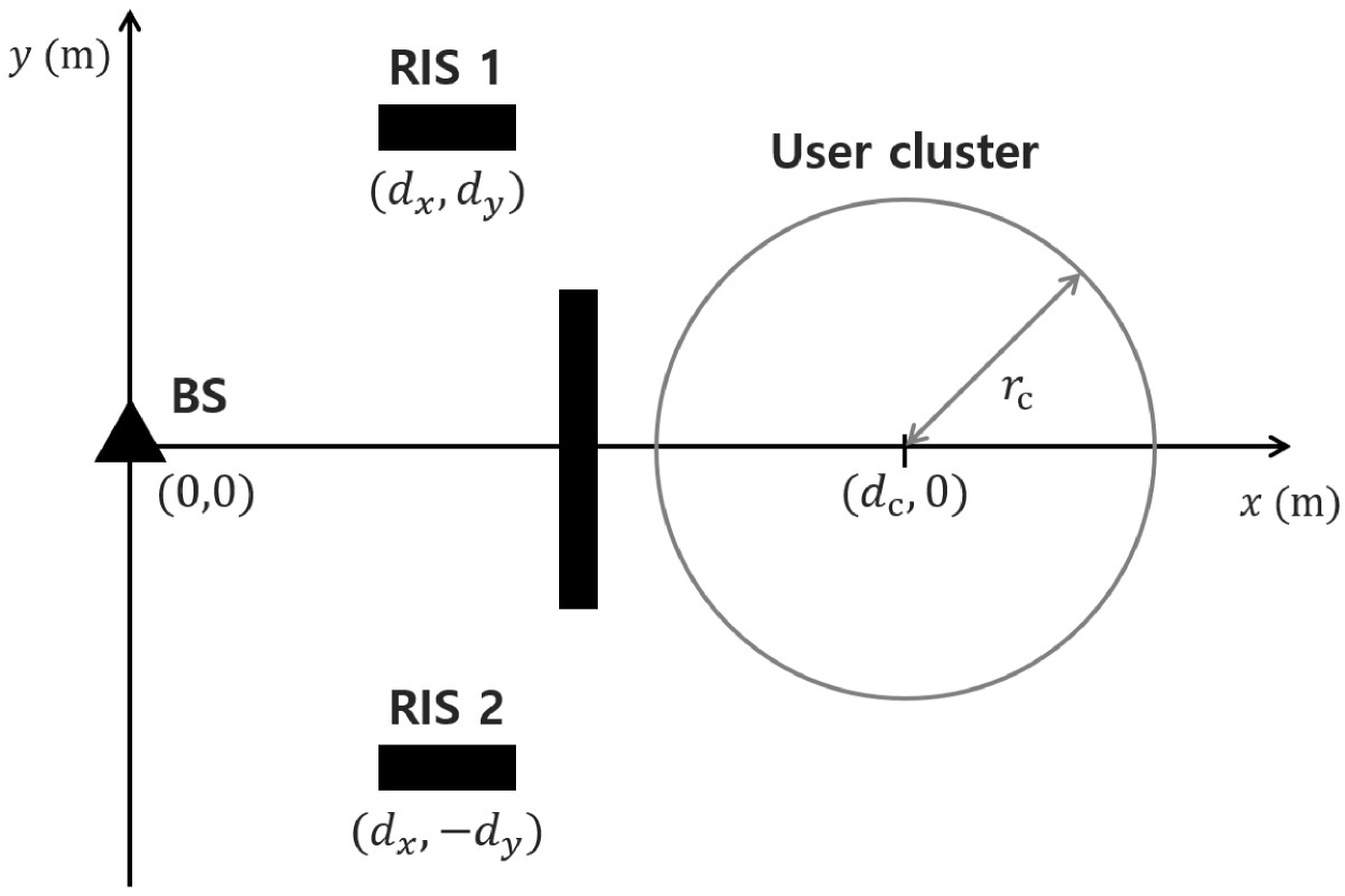
Figure 2: A schematic of the multiuser network with two RISs

Considering that the system operates at a 28 GHz carrier frequency, we adopt the mmWave pathloss model [43]. Thus, the pathloss in dB is given by

$${\sf PL}(d)=\alpha_{\sf PL}+\beta_{\sf PL}10\log_{10}d+\chi\ [{\rm dB}],$$ (60)

where $d$ denotes the link distance in meter, $\chi\sim\mbox{$\mathcal{N}$}(0,\sigma_{s}^{2})$ is the log-normal shadowing. This pathloss model is applied to the path gain terms in (54) and (59). According to [43], the experimental data for 28 GHz channels and 1 GHz bandwidth indicates that the parameters in (60) are set to be $\alpha_{\sf PL}=61.4,\beta_{\sf PL}=2,\sigma_{s}^{2}=5.8$ dB. Additionally, the noise power is given by

$$P_{\sf noise}=-174+10\log_{10}W+n_{f}\ [{\rm dBm}],$$ (61)

where $W$ and $n_{f}$ are the channel bandwidth and noise figure at the BS. Assuming the normalized noise variance, i.e., $\sigma^{2}=1$, the large-scale path gain is computed also from normalizing the pathloss as

$$\gamma=-({\sf PL}(d)+P_{\sf noise})\ [{\rm dB}].$$ (62)

In (61), we consider $W\!=\!1$ GHz and $n_{f}\!=\!5$ dB. In the considered channel model, we set $\Delta_{\sf B}/\lambda_{c}\!=\!\Delta_{y}/\lambda_{c}\!=\!\Delta_{z}/\lambda_{c}\!=\!0.5$, and randomly generate the signal azimuth and elevation angles of the UPA as $(\varphi^{a}_{k,\ell},\varphi^{a}_{\ell})\in[-\pi,\pi]$ and $(\varphi^{e}_{\ell},\varphi^{e}_{k,\ell})\in[-\pi/2,\pi/2]$, and also the AoD of the ULA as $\vartheta^{\sf B}_{\ell}\in[0,\pi],\;\forall\ell\in\mathcal{L},\forall k\in\mathcal{K}$. For the channel estimation discussed in Section II-B, we set $T_{\sf UL}=MK$ and $\rho_{\sf UL}=0\;{\rm dBm}$.

In the simulations, we consider the MU-MIMO downlink system assisted with $L=2$ RISs unless mentioned otherwise. To illustrate the location of the entities in the considered system, we apply a two-dimensional (2D) coordinate system as shown in Fig. 2. The BS and origin of the circle are set as $(0,0)$ and $(d_{{\rm cir}},0)$, respectively. The users are randomly generated within $r_{\sf c}=20$ m radius of a circle, and the distance between the BS and the origin of the circle is set to be $d_{{\sf c}}=60$ m. The locations of RIS 1 and RIS 2 are set as $(d_{x},d_{y})$ and $(d_{x},-d_{y})$, where $d_{x}=d_{y}=20$ m, and the number of the spatial paths are set to be ${\color[rgb]{0,0,0}L_{\sf BR}=L_{\sf RU}=2}$ unless mentioned otherwise.

IV-B Performance Evaluation

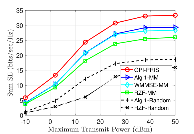
Figure 3: The sum SE versus the maximum transmit power $P$ dBm for $N=16$ BS antennas, $K=4$ users, and $M=64$ RIS phase shifts.

1) Maximum Transmit Power vs. Sum SE: We evaluate the performance of the proposed algorithm with respect to the maximum transmit power $P$ for $N\!=\!16$, $K\!=\!4$, $M\!=\!64$ ($M_{y}\!=\!8$, $M_{z}\!=\!8$). As shown in Fig. 3, our method achieves substantial SE gains compared to all baselines across all transmit power regimes. Specifically, the proposed algorithm exhibits a significant performance improvement over the random-phase scheme. In addition, RZF, due to its linear nature, shows limited performance in maximizing the sum SE. This observation suggests that SE performance can be effectively enhanced through RIS phase shift optimization. In terms of RIS phase shift optimization, our method shows significant performance improvement compared to Alg 1-MM by finding a superior local optimal solution. Consequently, our method demonstrates the effective joint optimization for the precoder and RIS phase shift over different transmit power regime.

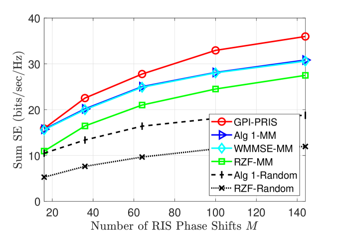
Figure 4: The sum SE versus the number of RIS phase shifts $M$ for $N=16$ BS antennas, $K=4$ users, and $P=20$ dBm maximum transmit power.

2) Number of RIS Phase Shifts vs. Sum SE: We compare the performance of the proposed algorithm and baselines in terms of the number of RIS phase shifts $M$ with $M_{y}\!=\!M_{z}$. We depict the comparison results in Fig. 4 for $N\!=\!16$, $K\!=\!4$, and $P\!=\!20$ dBm. In Fig. 4, the proposed algorithm achieves the highest performance across all tested numbers of RIS elements. Fig. 4 also shows a significant increase in the SE performance with increasing $M$ for our method. In contrast, the baseline methods show only marginal improvements with increasing $M$. This improvement is attributed to the efficient transmission strategy by properly incorporating the partial CSIT and identifying a superior local optimal point the regularized GPI method. These results emphasize the suitability of the proposed algorithm for high-speed data communications and coverage expansion by employing multiple RISs with a number of elements.

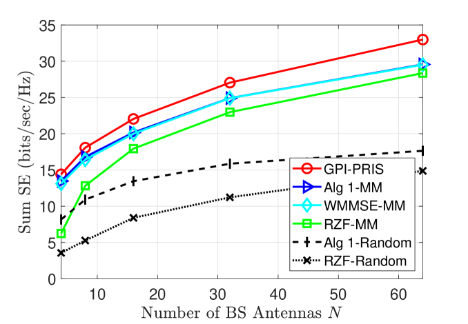
Figure 5: The sum SE versus the number of BS antennas $N$ for $M=32$ RIS phase shifts, $K=4$ users, and $P=20$ dBm maximum transmit power.

3) Number of BS antennas vs. Sum SE: We evaluate the sum SE with respect to the number of BS antennas for $K\!=\!4$, $M\!=\!32\;(M_{y}\!=\!8,M_{z}\!=\!4)$, and $P\!=\!20$ dBm. In Fig. 5, it is shown that the proposed algorithm also achieves the highest SE performance across all tested numbers of $N$. We note that RZF-MM achieves comparable performance to other baselines at $N\!=\!64$ due to sufficient degree-of-freedom (DoF). While all baselines show similar performance trends in terms of $N$, a performance gap exists between our method and the baselines, which becomes more pronounced with higher $N$. Similar to the observation from Fig. 4, fully leveraging the partial CSIT and finding a superior local optimal point through the GPI method contribute to this performance improvement.

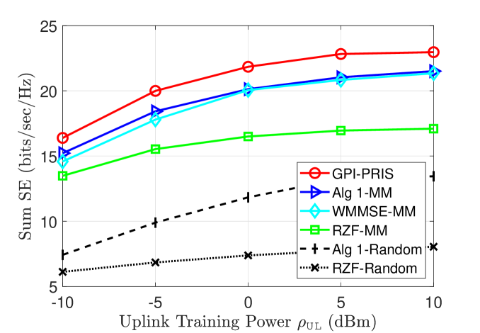
Figure 6: The sum SE versus the channel estimation parameter $\rho_{\sf UL}$ for $N=16$ BS antennas, $K=4$ users, $M=32$ RIS phase shifts, and $P=20$ dBm maximum transmit power.

4) CSIT Accuracy: We investigate the sum SE in relation to the accuracy of CSIT. In this simulation, we consider $N=16$, $K=4$, $M=32$, and $P=20\;{\rm dBm}$. Note that the increased value of $\rho_{\sf UL}$ directly correlates with improved channel estimation accuracy. As expected, Fig. 6 shows an increasing SE with $\rho_{\sf UL}$. Fig. 6 demonstrates that our algorithm achieves the highest SE performance over different $\rho_{\sf UL}$. We also observe that there exists performance gap between Alg 1-MM and WMMSE-MM in the low $\rho_{\sf UL}$ regime from Fig. 6. This performance gap arises from Algorithm 1 that the error covariance is embedded to effectively handle channel estimation errors. For such a reason, GPI-PRIS has robust performance in the coarse channel estimation environment owing to both Algorithm 1 and Algorithm 2 utilizing the error covariance. Thus, leveraging our GPI-based optimization framework and incorporating the error covariance-embedded transmission strategy, our algorithm offers robust joint beamforming solutions that maintain the highest performance.

$\begin{array}[]{c}{\leavevmode\resizebox{195.12767pt}{}{\includegraphics{Figures/Fig_converge_M32.pdf}}}\\ \mbox{\small(a) $M=32$}\end{array}$

$\begin{array}[]{c}{\leavevmode\resizebox{195.12767pt}{}{\includegraphics{Figures/Fig_converge_M64.pdf}}}\\ \mbox{\small(b) $M=64$}\end{array}$

Figure 7: Convergence behavior of GPI-PRIS (Algorithm 3) for $N=16$ BS antennas, $K=4$ users, $M\in\{32,64\}$ RIS phase shifts, and $P\in\{0,20,40\}$ dBm maximum transmit power.

5) Convergence Behavior: To identify the convergence behavior of the proposed algorithm, we evaluate the proposed GPI-PRIS regarding the sum SE versus the number of outer iterations for the various transmit power regime as $P\in\{0,20,40\}$ dBm. We assume $N=16$ and $K=4$ in both $M=32$ and $M=64$ cases. For the $M\!=\!32$ ($M_{y}\!=\!8$, $M_{z}\!=\!4$) case, Fig. 7(a) illustrates that the proposed algorithm converges within 11 iterations. Additionally, we examine a larger scale RIS configuration with $M\!=\!64$ ($M_{y}\!=\!8$, $M_{z}\!=\!8$) as depicted in Fig. 7(b). This scenario demonstrates that the proposed algorithm requires 13 iteration to converge. The increase in the iteration counts can be attributed to the expanded search space for the number of RIS elements. The results underscore that the proposed algorithm achieves fast convergence.

6) Regularization Behavior: We analyze the regularization behavior of our algorithms based on a GPI method for $N\!=\!16$, $K\!=\!4$, and $M\!=\!32$ $(M_{y}\!=\!8,M_{z}\!=\!4)$ with the following metric:

$${\rm NMSE}\left(\sqrt{LM}|{\bf w}^{\star}|-{\bf 1}\right),$$ (63)

where ${\rm NMSE}(\cdot)$ denotes a normalized mean square error (NMSE) function and ${\bf 1}$ denotes a vector whose elements are one with proper dimension. To study the impact of the regularization parameter $\mu\in[0,100]$, we employ the linear search method with $N_{\mu}=15$ linearly spaced points. Fig. 8(a) illustrates that NMSE decreases for all transmit power regimes as $\mu$ increases. This behavior can be attributed to the increasing dominance of the penalty term in the objective function with higher $\mu$ values, which effectively enforces the unit-modulus constraint on the RIS phase shifts. Consequently, as $\mu$ increases, NMSE approaches zero, which indicates that the unit-modulus constraint is nearly satisfied.

$\begin{array}[]{c}{\leavevmode\resizebox{195.12767pt}{}{\includegraphics{Figures/Fig_Reg_NMSE_M32.pdf}}}\\ \mbox{\small(a) NMSE}\end{array}$

$\begin{array}[]{c}{\leavevmode\resizebox{195.12767pt}{}{\includegraphics{Figures/Fig_Reg_SE_M32.pdf}}}\\ \mbox{\small(b) Sum SE}\end{array}$

Figure 8: The results in terms of the regularization parameter $\mu$ for $N=16$ BS antennas, $K=4$ users, $M=32$ RIS phase shifts, and $P\in\{0,20,40\}$ dBm maximum transmit power.

We also verify the SE performance with respect to the value of $\mu$ with the same scenario considered above. In Fig. 8(b), it is observed that the sum SE is effectively maximized using the line search method. Let $\bar{\boldsymbol{\phi}}_{\sf d}\!=\![{\boldsymbol{\phi}}_{{\sf d},1},\!\cdots\!,{\boldsymbol{\phi}}_{{\sf d},L}]$ be a deviation from the optimized RIS elements prior to projecting onto the feasible solution set, which is defined as $\bar{\boldsymbol{\phi}}_{\sf d}\!=\!e^{j{\rm arg}({\bf w}^{\star})}\!-\!\sqrt{LM}{\bf w}^{\star}$. At low $P$, the deviation has marginal impact on SE performance, since the AWGN power is more dominant than the possible errors caused by such deviation. In this regard, the optimization primarily focuses on maximizing the sum SE with little consideration of the unit-modulus constraint. At high $P$, the optimization prioritizes strict adherence to the constraint, and thus the optimal $\mu$ becomes larger. We note that depending on the transmit power, there exist optimal $\mu$. In addition, the sum SE reveals the low sensitivity around the optimal region. In this regard, the suitable value of $\mu$ can be pre-defined with respect to the transmit power, which further reduces the complexity of the proposed algorithm. Overall, we confirm that our approach enables a balanced trade-off in the regularized optimization problem over $P$.

$\begin{array}[]{c}{\leavevmode\resizebox{186.45673pt}{}{\includegraphics{Figures/Fig_MultipleL_SE.pdf}}}\\ \mbox{\small(a) Sum SE}\end{array}$ $\begin{array}[]{c}{\leavevmode\resizebox{186.45673pt}{}{\includegraphics{Figures/Fig_MultipleL_time.pdf}}}\\ \mbox{\small(b) Computation Time}\end{array}$

Figure 9: The comparison of the proposed algorithm and the baselines over the number of RISs $L$ with $N=32,K=12$, and ${\rm SNR}=20{\rm\;dB}$. The total number of RIS elements is fixed as $M_{\rm tot}=LM=144$.

7) Multi-RIS Scalability: We evaluate the sum SE in scalable RIS-aided systems by increasing $L$ and keeping the total number of deployed RIS elements $M_{\rm tot}=L\times M=144$. The values of $M_{y}$ and $M_{z}$ are determined such that $M_{\rm tot}/L=M_{y}\times M_{z}$. We consider $N=32$ and $K=12$. Here, we use a pre-determined $\mu$, and consider only the small-scale fading with both randomly distributed RISs and users while fixing all path-loss terms as 1 for simplicity. Hence, in this scenario, we use a signal-to-noise ratio (SNR) $P/\sigma^{2}$ which is set to be $P/\sigma^{2}=20\;{\rm dB}$ SNR. With fixed $M_{\rm tot}$, Fig. 9(a) demonstrates performance improvement as $L$ increases, reaching an optimal configuration at $L=16$ from the considered cases. We note that GPI-PRIS achieves the highest SE performance across different values of $L$.

Unlike the baseline that requires the complexity of $\mathcal{O}(M_{\rm tot}^{2})$, which represents a constant complexity order regarding $L$, our algorithm achieves complexity order of $\mathcal{O}(M_{\rm tot}^{3}/L^{2})$ with respect to $L$ as discussed in Remark 1. To numerically verify this, we assess computation time in MATLAB with the workstation equipped with i9-13900K CPU, RTX 4080 GPU, and 64 GB RAM. Fig. 9(b) shows that GPI-PRIS exhibits a decreasing trend as $L$ increases, whereas Alg 1-MM remains nearly constant, which aligns with our discussion. We remark that at the best $L=16$, GPI-PRIS achieves about $10\%$ SE gain while requiring only about $30\%$ computation time of Alg-1-MM. We omit the comparison with WMMSE-MM due to its extensively high computation time. For example, WMMSE-MM attains similar SE performance with Alg 1-MM, but its the computation time is $350.96$ sec for $L=16$, which is $123\times$ higher than that of GPI-PRIS. Overall, our algorithm demonstrates both the superior SE performance and multi-RIS scalability compared to the baselines, which can provide significant benefit of multi-RIS systems for future wireless communications networks.

V Conclusion

In this paper, we proposed the scalable and effective beamforming design for multi-RIS-aided systems under imperfect CSIT. Aiming to maximize the sum SE, we reformulated the optimization problem by deriving a lower bound of the instantaneous SE with partial CSIT. Dividing the problem into two subproblems, we developed the unified GPI-based optimization framework with regularization that identifies a superior local optimal solution. In particular, by leveraging the block diagonality of the GPI matrices, the proposed algorithm achieves multi-RIS scalability with respect to the number of RISs $L$, i.e., $\sim\mathcal{O}(1/L^{2})$ for the fixed total RIS elements case. Through simulations, we showed that our method not only outperforms conventional methods in terms of SE but also demonstrates significant computational scalability with respect to the number of RISs $L$, making it suitable for large-scale multi-RIS deployments under imperfect CSIT. Therefore, this work contributes both a robust and efficient beamforming design for practical multi-RIS-aided communication systems.

Appendix A Proof of Lemma 1

According to the stationary condition, the stationary points need to satisfy $\partial\mbox{$\mathcal{L}$}_{\sf BS}(\bar{\bf f})/\partial\bar{\bf f}^{\sf H}=0$. Thus, we take the partial derivative of $\mbox{$\mathcal{L}$}_{\sf BS}(\bar{\bf f})$ with respect to ${\bf\bar{f}}$ and set it to be zero. By using the derivative of the Rayleigh quotient form as

$$\frac{\partial\left(\frac{{\bf\bar{f}}^{\sf H}{{\bf A}}_{k}\bar{\bf f}}{{\bf\bar{f}}^{\sf H}{{\bf B}}_{k}\bar{\bf f}}\right)}{\partial\bar{\bf f}^{\sf H}}=2\left(\frac{{\bf\bar{f}}^{\sf H}{{\bf A}}_{k}\bar{\bf f}}{{\bf\bar{f}}^{\sf H}{{\bf B}}_{k}\bar{\bf f}}\right)\left[\frac{{{\bf A}}_{k}\bar{\bf f}}{{\bf\bar{f}}^{\sf H}{{\bf A}}_{k}\bar{\bf f}}-\frac{{{\bf B}}_{k}\bar{\bf f}}{{\bf\bar{f}}^{\sf H}{{\bf B}}_{k}\bar{\bf f}}\right],$$ (64)

we can calculate the partial derivative of $\mbox{$\mathcal{L}$}_{\sf BS}(\bar{\bf f})$ in (27) as

$$\frac{\partial\mbox{$\mathcal{L}$}_{\sf BS}(\bar{\bf f})}{\partial\bar{\bf f}^{\sf H}}=\sum_{k=1}^{K}\frac{2}{\ln 2}\left(\frac{{{\bf A}}_{k}\bar{\bf f}}{{\bf\bar{f}}^{\sf H}{{\bf A}}_{k}\bar{\bf f}}-\frac{{{\bf B}}_{k}\bar{\bf f}}{{\bf\bar{f}}^{\sf H}{{\bf B}}_{k}\bar{\bf f}}\right).$$ (65)

Using (65) the stationary condition holds if

$$\sum_{k=1}^{K}\left(\frac{{\bf A}_{k}}{{\bf\bar{f}}^{\sf H}{\bf A}_{k}\bar{\bf f}}\right)\bar{\bf f}=\sum_{k=1}^{K}\left(\frac{{\bf B}_{k}}{{\bf\bar{f}}^{\sf H}{\bf B}_{k}\bar{\bf f}}\right)\bar{\bf f}.$$ (66)

The stationary condition can be regarded as the generalized eigenvalue problem with its corresponding matrices $\bar{{\bf A}}({\bf f})$ and $\bar{{\bf B}}({\bf f})$ defined in (29) and (30):

$$\bar{{\bf A}}(\bar{\bf f})\bar{\bf f}=\lambda_{\sf BS}(\bar{\bf f})\bar{{\bf B}}(\bar{\bf f})\bar{\bf f}.$$ (67)

Here, $\lambda_{{\sf BS},\sf{num}}(\bar{{\bf f}})$ and $\lambda_{{\sf BS},\sf{den}}(\bar{{\bf f}})$ can be any function such that $\lambda_{\sf BS}(\bar{{\bf f}})=\lambda_{{\sf BS},\sf{num}}(\bar{{\bf f}})/\lambda_{{\sf BS},\sf{den}}(\bar{{\bf f}})$. We note that $\bar{{\bf B}}({\bf w})$ can be considered to be invertible. This completes the proof. $\blacksquare$

Appendix B Proof of Corollary 2

Using the LogSumExp approach in III-B, the Lagrangian function of the problem (50) is expressed as $\tilde{\mbox{$\mathcal{L}$}}_{\sf RIS}({\bf w})$ in (48). To find the stationary points, we take derivatives of (48) as

$$\frac{\partial\tilde{\mathcal{L}}_{\sf RIS}({{\bf w}})}{\partial{{\bf w}}^{\sf H}}=\frac{2}{R_{\Sigma}\ln{2}}\sum_{k=1}^{K}\left[\frac{{\bf C}_{k}{{\bf w}}}{{{\bf w}}^{\sf H}{\bf C}_{k}{{\bf w}}}-\frac{{\bf D}_{k}{{\bf w}}}{{{\bf w}}^{\sf H}{\bf D}_{k}{{\bf w}}}\right]$$

$$-\frac{2\mu}{\tau}\frac{\sum_{m=1}^{M}{\bf X}_{m}{\bf w}e^{{{\bf w}}^{\sf H}{\bf X}_{m}{{\bf w}}}}{\sum_{m=1}^{M}e^{{{\bf w}}^{\sf H}{\bf X}_{m}{{\bf w}}}}+\frac{2\mu}{\tau}\frac{\sum_{m=1}^{M}{\bf X}_{m}{\bf w}e^{\frac{{{\bf w}}^{\sf H}{\bf X}_{m}{{\bf w}}}{-\alpha_{2}}}}{\sum_{m=1}^{M}e^{\frac{{{\bf w}}^{\sf H}{\bf X}_{m}{{\bf w}}}{-\alpha_{2}}}}.$$ (68)

Similar to the proof of Lemma 1, we find the condition for $\partial\tilde{\mbox{$\mathcal{L}$}}_{\sf RIS}({{\bf w}})/\partial{{\bf w}}^{\sf H}=0$. Consequently, from (B), the stationary condition can be reformulated as

$$\bar{{\bf C}}({\bf w}){\bf w}=\lambda_{\sf RIS}({\bf w})\bar{{\bf D}}({\bf w}){\bf w},$$ (69)

where its corresponding matrices $\bar{{\bf C}}({\bf w})$ and $\bar{{\bf D}}({\bf w})$ are defined in (2) and (2). Here, $\lambda_{{\sf RIS},\sf{num}}({\bf w})$ and $\lambda_{{\sf RIS},\sf{den}}({\bf w})$ can be any function such that $\lambda_{\sf RIS}({\bf w})=\lambda_{{\sf RIS},\sf{num}}({\bf w})/\lambda_{{\sf RIS},\sf{den}}({\bf w})$. We note that $\bar{{\bf D}}({\bf w})$ can be considered to be invertible. $\blacksquare$

References

- [1] Q. Wu and R. Zhang, “Towards smart and reconfigurable environment: Intelligent reflecting surface aided wireless network,” IEEE Commun. Mag., vol. 58, no. 1, pp. 106–112, 2019.
- [2] Y. Liu, X. Liu, X. Mu, T. Hou, J. Xu, M. Di Renzo, and N. Al-Dhahir, “Reconfigurable intelligent surfaces: Principles and opportunities,” IEEE Comm. Surveys & Tutorials, vol. 23, no. 3, pp. 1546–1577, 2021.
- [3] R. W. Heath, N. Gonzalez-Prelcic, S. Rangan, W. Roh, and A. M. Sayeed, “An overview of signal processing techniques for millimeter wave MIMO systems,” IEEE J. Sel. Topics Signal Process., vol. 10, no. 3, pp. 436–453, 2016.
- [4] P. Wang, J. Fang, L. Dai, and H. Li, “Joint transceiver and large intelligent surface design for massive MIMO mmWave systems,” IEEE Trans. Wireless Commun., vol. 20, no. 2, pp. 1052–1064, 2020.
- [5] Z. Li, H. Hu, J. Zhang, and J. Zhang, “RIS-assisted mmWave networks with random blockages: Fewer large RISs or more small RISs?” IEEE Trans. Wireless Commun., vol. 22, no. 2, pp. 986–1000, 2022.
- [6] Y. Lin, S. Jin, M. Matthaiou, and X. You, “Channel estimation and user localization for IRS-assisted MIMO-OFDM systems,” IEEE Trans. Wireless Commun., vol. 21, no. 4, pp. 2320–2335, 2021.
- [7] J. Yao, J. Xu, W. Xu, D. W. K. Ng, C. Yuen, and X. You, “Robust beamforming design for RIS-aided cell-free systems with CSI uncertainties and capacity-limited backhaul,” IEEE Trans. Commun., vol. 71, no. 8, pp. 4636–4649, 2023.
- [8] W. Mei, B. Zheng, C. You, and R. Zhang, “Intelligent reflecting surface-aided wireless networks: From single-reflection to multireflection design and optimization,” Proc. of the IEEE, vol. 110, no. 9, pp. 1380–1400, 2022.
- [9] Y. Han, S. Zhang, L. Duan, and R. Zhang, “Cooperative double-IRS aided communication: Beamforming design and power scaling,” IEEE Wireless Commun. Lett., vol. 9, no. 8, pp. 1206–1210, 2020.
- [10] M. Aldababsa, A. M. Salhab, A. A. Nasir, M. H. Samuh, and D. B. da Costa, “Multiple RISs-aided networks: Performance analysis and optimization,” IEEE Trans. Veh. Technol., vol. 72, no. 6, pp. 7545–7559, 2023.
- [11] G.-H. Li, D.-W. Yue, S.-N. Jin, and Q. Hu, “Performance analysis of multi-RIS-aided mmWave MIMO systems using Poisson point processes,” IEEE Signal Process. Lett., 2023.
- [12] B. Al-Nahhas, M. Obeed, A. Chaaban, and M. J. Hossain, “Performance of multi-RIS-aided cell-free massive MIMO: Do more RISs always help?” IEEE Trans. on Commun., 2024.
- [13] Z. Li, M. Hua, Q. Wang, and Q. Song, “Weighted sum-rate maximization for multi-IRS aided cooperative transmission,” IEEE Wireless Commun. Lett., vol. 9, no. 10, pp. 1620–1624, 2020.
- [14] C. Pan, H. Ren, K. Wang, W. Xu, M. Elkashlan, A. Nallanathan, and L. Hanzo, “Multicell MIMO communications relying on intelligent reflecting surfaces,” IEEE Trans. Wireless Commun., vol. 19, no. 8, pp. 5218–5233, 2020.
- [15] H. Huang, Y. Zhang, H. Zhang, Z. Zhao, C. Zhang, and Z. Han, “Multi-IRS-aided millimeter-wave multi-user MISO systems for power minimization using generalized Benders decomposition,” IEEE Trans. Wireless Commun., 2023.
- [16] H. Do, N. Lee, and A. Lozano, “Line-of-sight MIMO via intelligent reflecting surface,” IEEE Trans. Wireless Commun., 2022.
- [17] F. Liu, Y. Cui, C. Masouros, J. Xu, T. X. Han, Y. C. Eldar, and S. Buzzi, “Integrated sensing and communications: Toward dual-functional wireless networks for 6G and beyond,” IEEE J. Sel. Areas Commun., vol. 40, no. 6, pp. 1728–1767, 2022.
- [18] Z. Zheng, W. Jing, Z. Lu, Q. Wu, H. Zhang, and D. Gesbert, “Cooperative multi-satellite and multi-RIS beamforming: Enhancing LEO SatCom and mitigating LEO-GEO intersystem interference,” IEEE J. Sel. Areas Commun., 2024.
- [19] X. Li, H. Wang, Y. Chen, and S. Sheng, “Joint resource allocation and reflecting precoding design for RIS-assisted ISAC systems,” IEEE Wireless Commun. Lett., 2024.
- [20] M. Toka, B. Lee, J. Seong, A. Kaushik, J. Lee, J. Lee, N. Lee, W. Shin, and H. V. Poor, “RIS-Empowered LEO satellite networks for 6G: promising usage scenarios and future directions,” arXiv preprint arXiv:2402.07381, 2024.
- [21] G. Zhou, C. Pan, H. Ren, K. Wang, and A. Nallanathan, “A framework of robust transmission design for IRS-aided MISO communications with imperfect cascaded channels,” IEEE Trans. Signal Process., vol. 68, pp. 5092–5106, 2020.
- [22] Y. Omid, S. M. Shahabi, C. Pan, Y. Deng, and A. Nallanathan, “Low-complexity robust beamforming design for IRS-aided MISO systems with imperfect channels,” IEEE Commun. Lett., vol. 25, no. 5, pp. 1697–1701, 2021.
- [23] P. Zeng, D. Qiao, H. Qian, and Q. Wu, “Joint beamforming design for IRS aided multiuser MIMO with imperfect CSI,” IEEE Trans. Veh. Technol., vol. 71, no. 10, pp. 10 729–10 743, 2022.
- [24] Y. Omid, S. M. Shahabi, C. Pan, Y. Deng, and A. Nallanathan, “Robust beamforming design for an IRS-aided NOMA communication system with CSI uncertainty,” IEEE Trans. Wireless Commun., vol. 23, no. 2, pp. 874–889, 2023.
- [25] W. Jiang, P. Xiong, J. Nie, Z. Ding, C. Pan, and Z. Xiong, “Robust design of IRS-aided multi-group multicast system with imperfect CSI,” IEEE Trans. Wireless Commun., 2023.
- [26] G. Zhou, C. Pan, H. Ren, K. Wang, and A. Nallanathan, “Intelligent reflecting surface aided multigroup multicast MISO communication systems,” IEEE Trans. Signal Process., vol. 68, pp. 3236–3251, 2020.
- [27] S. Zargari, A. Khalili, and R. Zhang, “Energy efficiency maximization via joint active and passive beamforming design for multiuser MISO IRS-aided SWIPT,” IEEE Wireless Commun. Lett., vol. 10, no. 3, pp. 557–561, 2020.
- [28] Y. Xiu, Y. Zhao, Y. Liu, J. Zhao, O. Yagan, and N. Wei, “IRS-assisted millimeter wave communications: Joint power allocation and beamforming design,” in Proc. IEEE Wireless Commun. and Netw. Conf. IEEE, 2021, pp. 1–6.
- [29] C. Pan, G. Zhou, K. Zhi, S. Hong, T. Wu, Y. Pan, H. Ren, M. Di Renzo, A. L. Swindlehurst, R. Zhang et al., “An overview of signal processing techniques for RIS/IRS-aided wireless systems,” IEEE J. Sel. Topics Signal Process., 2022.
- [30] E. Shtaiwi, H. Zhang, A. Abdelhadi, A. L. Swindlehurst, Z. Han, and H. V. Poor, “Sum-rate maximization for RIS-assisted integrated sensing and communication systems with manifold optimization,” IEEE Trans. Commun., 2023.
- [31] J. Wang, S. Gong, Q. Wu, and S. Ma, “RIS-aided MIMO systems with hardware impairments: Robust beamforming design and analysis,” IEEE Trans. Wireless Commun., vol. 22, no. 10, pp. 6914–6929, 2023.
- [32] S.-H. Yoon, B. Lim, M. Vu, and Y.-C. Ko, “Joint user selection and beamforming design for multi-IRS aided internet-of-things networks,” IEEE Trans. Veh. Technol., 2023.
- [33] J. Choi, N. Lee, S.-N. Hong, and G. Caire, “Joint user selection, power allocation, and precoding design with imperfect CSIT for multi-cell MU-MIMO downlink systems,” IEEE Trans. Wireless Commun., vol. 19, no. 1, pp. 162–176, 2019.
- [34] N. K. Kundu and M. R. McKay, “Channel estimation for reconfigurable intelligent surface aided MISO communications: From LMMSE to deep learning solutions,” IEEE Open Jour. of the Commun. Society, vol. 2, pp. 471–487, 2021.
- [35] C. Xu, J. An, T. Bai, S. Sugiura, R. G. Maunder, Z. Wang, L.-L. Yang, and L. Hanzo, “Channel estimation for reconfigurable intelligent surface assisted high-mobility wireless systems,” IEEE Trans. Veh. Technol., vol. 72, no. 1, pp. 718–734, 2022.
- [36] X. Wei, D. Shen, and L. Dai, “Channel estimation for RIS assisted wireless communications—Part I: Fundamentals, solutions, and future opportunities,” IEEE Commun. Lett., vol. 25, no. 5, pp. 1398–1402, 2021.
- [37] H. Joudeh and B. Clerckx, “Sum-rate maximization for linearly precoded downlink multiuser MISO systems with partial CSIT: A rate-splitting approach,” IEEE Trans. Commun., vol. 64, no. 11, pp. 4847–4861, 2016.
- [38] S. Lee, E. Choi, and J. Choi, “Max-Min Fairness Precoding for Physical Layer Security With Partial Channel Knowledge,” IEEE Wireless Commun. Lett., vol. 12, no. 9, pp. 1637–1641, 2023.
- [39] J. Choi, J. Park, and N. Lee, “Energy efficiency maximization precoding for quantized massive MIMO systems,” IEEE Trans. Wireless Commun., vol. 21, no. 9, pp. 6803–6817, 2022.
- [40] C. Shen and H. Li, “On the dual formulation of boosting algorithms,” IEEE Trans. Pattern Analysis and Machine Intelligence, vol. 32, no. 12, pp. 2216–2231, 2010.
- [41] Q. Shi, M. Razaviyayn, Z.-Q. Luo, and C. He, “An iteratively weighted MMSE approach to distributed sum-utility maximization for a MIMO interfering broadcast channel,” IEEE Trans. Signal Process., vol. 59, no. 9, pp. 4331–4340, 2011.
- [42] A. A. Saleh and R. Valenzuela, “A statistical model for indoor multipath propagation,” IEEE J. Sel. Areas Commun., vol. 5, no. 2, pp. 128–137, 1987.
- [43] M. R. Akdeniz, Y. Liu, M. K. Samimi, S. Sun, S. Rangan, T. S. Rappaport, and E. Erkip, “Millimeter wave channel modeling and cellular capacity evaluation,” IEEE J. Sel. Areas Commun., vol. 32, no. 6, pp. 1164–1179, 2014.