Forecast constraints on the axion-photon coupling from interstellar medium heating

Abstract

In interstellar media characterized by a nonrelativistic plasma of electrons and heavy ions, we study the effect of axion dark matter coupled to photons on the dynamics of an electric field. In particular, we assume the presence of a background magnetic field aligned in a specific direction. We show that there is an energy transfer from the oscillating axion field to photons and then to the plasma induced by forced resonance. This resonance is most prominent for the axion mass $m_{\phi}$ equivalent to the plasma frequency $\omega_{p}$. Requiring that the heating rate of the interstellar medium caused by the energy transfer does not exceed the observed astrophysical cooling rate, we place forecast constraints on the axion-photon coupling $g$ for several different amplitudes of the background magnetic field $B_{0}$. By choosing a typical value $B_{0}=10^{-5}$ G, we find that, for the resonance mass $m_{\phi}=\omega_{p}$, the upper limit of $g$ can be stronger than those derived from other measurements in the literature. With increased values of $B_{0}$, it is possible to put more stringent constraints on $g$ for a wider range of the axion mass away from the resonance point.

I Introduction

The existence of a pseudo-Nambu Goldstone axion was originally introduced to address the strong CP problem in quantum chromodynamics (QCD) [1, 2, 3]. The mass of QCD axions is related to the axion decay constant $f$, as $m_{\phi}\simeq 5.7\times 10^{-6}~{\rm eV}\,(10^{12}~{\rm GeV}/f)$ [4]. The original model, which is not experimentally viable, was generalized to include heavy quarks [5, 6] or an additional Higgs field [7, 8]. The QCD axion in such extended versions can be light and stable for large $f$, being a good candidate for dark matter [9, 10, 11, 11] (see Refs. [12, 13, 14, 15, 16, 17] for reviews). In the context of string theory, ultralight axions can arise as Kaluza-Klein zero modes of anti-symmetric form fields [18, 19, 20]. The mass of string axions can span over a vast range $10^{-33}\,{\rm eV}\lesssim m_{\phi}\lesssim 10^{-10}$ eV, depending on the compactification scheme [21, 22, 23, 24, 25].

An axion $\phi$ may interact with photons through the Chern-Simons coupling ${\cal L}=-g\phi F_{\mu\nu}\widetilde{F}^{\mu\nu}/4$, where $g$ is a coupling constant and $F_{\mu\nu}$ is an electromagnetic field strength with $\widetilde{F}^{\mu\nu}$ its Hodge dual. In terms of the electric field ${\bm{E}}$ and the magnetic field ${\bm{B}}$, this interaction can be interpreted as the inner product $-g\phi{\bm{E}}\cdot{\bm{B}}$. Since the conversion of axions to photons can occur in the presence of external magnetic fields [26], the laboratory experiments such as a “light-shining-through-walls” measurement [27] put upper limits on the coupling $g$. For the mass range $m_{\phi}\lesssim 10^{-4}$ eV, the ALPS collaboration has constrained $g\leq 5\times 10^{-8}$ GeV^-1 [28]. By considering axions that are produced in the Sun and convert to $X$-rays in the magnetic field at the detector, the CAST [29] and IAXO [30] experiments placed the limit $g\leq 4\times 10^{-12}$ GeV^-1 for $m_{\phi}\leq 5\times 10^{-3}$ eV.

For light axions in the mass range $m_{\phi}\lesssim 10^{-10}$ eV, astrophysical observations put tightest bounds on the coupling constant $g$. The interaction ${\cal L}=-g\phi F_{\mu\nu}\widetilde{F}^{\mu\nu}/4$ allows the generation of axions in the stellar plasma through a Primakoff process [31, 32]. Axions can eventually convert into gamma rays in the magnetic field of the Milky Way. Since such gamma rays were not observed in the SN1987 event, this translates to the limit $g\leq 5.3\times 10^{-12}$ GeV^-1 for $m_{\phi}\leq 4.4\times 10^{-10}$ eV [33]. Similarly, axions generated inside stellar cores may convert into observable $X$-rays in the galactic magnetic field. The lack of observational evidence for $X$-rays from super star clusters leads to the limit $g\leq 3.6\times 10^{-12}$ GeV^-1 for $m_{\phi}\leq 5\times 10^{-11}$ eV [34]. If we consider magnetic white dwarfs (MWDs), the axion-photon coupling generates photons polarized parallel to the direction of the magnetic field. Polarization measurements of thermal radiation from MWDs have placed the bound $g\leq 5.4\times 10^{-12}$ GeV^-1 for $m_{\phi}\leq 3\times 10^{-7}$ eV [35]. In the mass range of so-called fuzzy dark matter [36], $m_{\phi}\sim 10^{-22}$ eV, axion searches by polarization plane rotation have been intensively studied [37, 38, 39], and the limit due to the decrease in the cosmic microwave background (CMB) polarization is $g\lesssim 10^{-13}~{\rm GeV}^{-1}\,(m_{\phi}/10^{-22}~{\rm eV})$ [40]. We also note that cosmic birefringence inferred from observations of CMB [41, 42] can constrain $g$ for the even lighter mass range $m_{\phi}\lesssim 10^{-26}$ eV [43, 44, 45, 46].

In this paper, we will propose a new method of probing the axion-photon coupling through the observed cooling rate of interstellar media. We consider a nonrelativistic plasma of electrons and heavy ions with the electron number density $n_{e}$. In the absence of the axion-photon coupling, the collective movement of electrons gives rise to the plasma oscillation of an electric field ${\bm{E}}$ with the angular frequency $\omega_{p}=\sqrt{n_{e}e^{2}/m_{e}}\simeq 10^{-11}\,{\rm eV}\,(n_{e}/0.1~{\rm cm}^{-3})^{1/2}$, where $e$ is the elementary charge and $m_{e}$ is the electron mass [47, 48]. For the typical number density $n_{e}\approx 0.1$ cm^-3 of dilute plasmas in interstellar media, the plasma frequency $\omega_{p}$ is of order $10^{-11}$ eV. The existence of heavy ions works to generate friction for the dynamics of electrons characterized by the damping rate $\nu$. Since we typically have $\nu\ll\omega_{p}$ for the interstellar plasma, the electric field exhibits damped oscillations with the decay time scale $\nu^{-1}$, which is much longer than the oscillating time scale $\omega_{p}^{-1}$.

If there are background magnetic fields in the interstellar region, the interaction ${\cal L}=-g\phi F_{\mu\nu}\widetilde{F}^{\mu\nu}/4$ can lead to the energy conversion from axions to photons in the plasma. The observations of interstellar magnetic fields in the galactic center suggest that their amplitudes may span in the range $B_{0}=10^{-5}~{\rm G}\sim 10^{-3}$ G [49]. In this paper, we will consider an external magnetic field ${\bm{B}}_{0}$ aligned in a specific direction and compute the heating rate of interstellar media induced by the axion-photon coupling. For this purpose, we deal with the axion as nonrelativistic dark matter oscillating around a minimum of the potential $V(\phi)=m_{\phi}^{2}\phi^{2}/2$. In the two-dimensional plane perpendicular to the direction of ${\bm{B}}_{0}$, the electric-field components still exhibit damped elliptic motions combined with the plasma oscillation and the cyclotron orbit in the normal manner. Along the direction of ${\bm{B}}_{0}$, however, we will show that the energy density of axions is converted to that of photons through forced resonance. In particular, the energy transfer rate $\dot{Q}$ is largest for the resonance mass $m_{\phi}$ equivalent to the plasma frequency $\omega_{p}$.

The observations of interstellar media like Leo T have constrained the cooling rate $\dot{C}$ as well as $\omega_{p}$ and $\nu$ [50, 51, 52, 53]. These astrophysical data can be used to probe the properties of dark matter [54, 55, 56, 57, 58, 59, 60, 61, 62, 63]. In our case, the heating rate $\dot{Q}$ induced by the axion-photon coupling should not exceed the observed cooling rate, which translates to the upper limit of $g$. At the resonance point, we will derive an analytic formula for the bound on $g$. For the plasma frequency in the range $10^{-12}~{\rm eV}\lesssim\omega_{p}\lesssim 10^{-10}~{\rm eV}$, the upper limit of $g$ at the resonance mass $m_{\phi}=\omega_{p}$ can be smaller than the MWD bound mentioned above by choosing the typical galactic magnetic field strength $B_{0}\approx 10^{-5}$ eV. In particular, the constraint on $g$ at $m_{\phi}=\omega_{p}$ tends to be stronger for smaller $\nu$ due to the occurrence of sharper resonance. With the increase of $B_{0}$, we can place tighter bounds on $g$ for a broader mass range away from the resonance point. While the precise magnetic field strengths have been unknown for interstellar media with observed cooling rates, upcoming observations may be able to put interesting constraints on $g$ for the mass range $10^{-15}~{\rm eV}\lesssim m_{\phi}\lesssim 10^{-7}~{\rm eV}$.

This paper is organized as follows. In Sec. II, we revisit the fundamental aspect of nonrelativistic plasmas and present observational constraints on the cooling rates of interstellar media known in the literature. In Sec. III, we consider the axion-photon coupling on the background of an external magnetic field in the plasma and derive solutions to the electric field under the approximation that spatial gradient terms are neglected relative to time-dependent terms. In Sec. IV, we compute the heating rate $\dot{Q}$ of interstellar media induced by forced resonance and put upper bounds on $g$ derived from the condition $\dot{Q}\leq\dot{C}$. Sec. V is devoted to conclusions. We use a natural unit in which the speed of light $c$, the reduced Planck constant $\hbar$, and the Boltzmann constant $k_{B}$ are 1. We adopt the metric signature $(-,+,+,+)$.

II Plasma in interstellar media

We consider an interstellar medium modeled by a nonrelativistic plasma of electrons and heavy ions with a thermal temperature $T$ [47, 48]. As in the standard plasma, the total charge of the system is assumed to be zero. Since the mass of ions is much larger than the electron mass, we ignore the ion velocity ${\bm{u}}_{i}$ relative to the electron velocity ${\bm{u}}_{e}$. Then, the total current is approximately given by

$$J^{\mu}=\left(0,{\bm{J}}\right)=\left(0,-n_{e}e\,{\bm{u}}_{e}\right)\,.$$ (1)

We deal with the electron (mass $m_{e}$ and charge $-e$) as a nonrelativistic particle. We also neglect general relativistic effects on the dynamics of electrons and electromagnetic fields. In the presence of an electric field ${\bm{E}}$ and a magnetic field ${\bm{B}}$, the Newtonian equation of motion for the electron yields

$$m_{e}\dot{{\bm{u}}}_{e}+m_{e}\left({\bm{u}}_{e}\cdot\nabla\right){\bm{u}}_{e}=-e\left({\bm{E}}+{\bm{u}}_{e}\times{\bm{B}}\right)-m_{e}\nu{\bm{u}}_{e}\,,$$ (2)

where a dot represents the derivative with respect to time $t$, $\nabla\equiv(\partial_{1},\partial_{2},\partial_{3})$ with $\partial_{i}\equiv\partial/\partial x^{i}$ ($x^{i}$ is the spatial position), and $\nu$ is a friction constant between electrons and ions. We can express $\nu$ in the form [55]

$$\nu=\frac{4\sqrt{2\pi}\alpha^{2}n_{e}}{6(m_{e}T^{3})^{1/2}}\ln\Lambda_{c}\simeq 1.2\times 10^{-22}~{\rm eV}\left(\frac{n_{e}}{0.1~{\rm cm}^{-3}}\right)\left(\frac{10^{4}~{\rm K}}{T}\right)^{3/2}\ln\Lambda_{c}\,,$$ (3)

where $\alpha=e^{2}/(4\pi)=1/137.036$ is the fine structure constant, and

$$\Lambda_{c}=\frac{4\pi T^{3}}{\alpha^{3}n_{e}}\simeq 2.7\times 10^{22}\left(\frac{0.1~{\rm cm}^{-3}}{n_{e}}\right)\left(\frac{T}{10^{4}~{\rm K}}\right)^{3}\,.$$ (4)

Since we are considering nonrelativistic electrons ($|{\bm{u}}_{e}|\ll 1$), the contribution $m_{e}\left({\bm{u}}_{e}\cdot\nabla\right){\bm{u}}_{e}$ to Eq. (2) can be neglected relative to the linear term in ${\bm{u}}_{e}$. Eq. (2) is approximately given by

$$m_{e}\dot{{\bm{u}}}_{e}\simeq-e\left({\bm{E}}+{\bm{u}}_{e}\times{\bm{B}}\right)-m_{e}\nu{\bm{u}}_{e}\,.$$ (5)

Assuming that $n_{e}$ is constant, the current ${\bm{J}}=-n_{e}e\,{\bm{u}}_{e}$ obeys

$$\dot{{\bm{J}}}\simeq\omega_{p}^{2}{\bm{E}}-\frac{e}{m_{e}}{\bm{J}}\times{\bm{B}}-\nu{\bm{J}}\,,$$ (6)

where

$$\omega_{p}=\sqrt{\frac{n_{e}e^{2}}{m_{e}}}\simeq 1.2\times 10^{-11}~{\rm eV}\left(\frac{n_{e}}{0.1~{\rm cm}^{-3}}\right)^{1/2}$$ (7)

is the plasma frequency.

In Table 1, we summarise the observed gas-rich astrophysical media and their associated values of $n_{e}$ and $T$. The plasma frequency $\omega_{p}$ and the electron-ion friction constant $\nu$ are computed according to the relations (7) and (3), respectively. It follows that $\omega_{p}\gg\nu$ for all these interstellar media. In the last column of Table 1, we also show the astrophysical cooling rate of the gas $\dot{C}$ for each medium. It is possible to exploit these observed values of $\dot{C}$ to put constraints on the coupling $g$ between axions and electromagnetic fields.

Interstellar media	$n_{e}$ (cm-3)	$T$ (K)	$\omega_{p}$ (eV)	$\nu$ (eV)	$\dot{C}$ (erg cm-3 s-1)
WNM (Leo T)	0.06	6100	$9.1\times 10^{-12}$	$7.6\times 10^{-21}$	$7\times 10^{-30}$
CNM (G33.4$-$8.0)	0.4	400	$2.3\times 10^{-11}$	$2.4\times 10^{-18}$	$1.46\times 10^{-27}$
MC (MW)	100	50	$3.7\times 10^{-10}$	$9.8\times 10^{-15}$	$3.16\times 10^{-24}$
CNM (MW)	30	100	$2.0\times 10^{-10}$	$1.2\times 10^{-15}$	$2.02\times 10^{-24}$
WNM (MW)	0.6	5000	$2.9\times 10^{-11}$	$9.7\times 10^{-20}$	$8.3\times 10^{-27}$
WIM (MW)	0.3	$10^{4}$	$2.0\times 10^{-11}$	$1.8\times 10^{-20}$	$5.4\times 10^{-26}$
HIM (MW)	0.003	106	$2.0\times 10^{-12}$	$2.5\times 10^{-25}$	$1.3\times 10^{-27}$

Table 1: Interstellar media, their electron number densities $n_{e}$, temperatures $T$, plasma frequencies $\omega_{p}$, electron-ion friction constants $\nu$, and cooling rates $\dot{C}$. The different phases are labeled as MC (molecular clouds), CNM (cold neutral medium), WNM (warm neutral medium),WIM (warm ionized medium), and HIM (hot ionized medium). MW denotes the data in the Milky Way and Leo T is a gas-rich dwarf galaxy. We take the observed values of $n_{e}$, $T$, and $\dot{C}$ from Ref. [53].

III Axions coupled to electromagnetic fields

As a candidate for dark matter, we consider a pseudo-scalar axion field $\phi$ with a constant mass $m_{\phi}$. The axion potential is given by $V(\phi)=m_{\phi}^{2}\phi^{2}/2$, which follows from $V(\phi)=m_{\phi}^{2}f^{2}[1-\cos(\phi/f)]$ as a leading-order term by the expansion around $\phi=0$. The axion is coupled to electromagnetic fields with the interacting Lagrangian $-g\phi F_{\mu\nu}\widetilde{F}^{\mu\nu}/4$, where $g$ is the coupling constant, $F_{\mu\nu}=\partial_{\mu}A_{\nu}-\partial_{\nu}A_{\mu}$ is the electromagnetic field strength of a four-dimensional gauge field $A_{\mu}$, and $\widetilde{F}^{\mu\nu}=F_{\alpha\beta}{\cal E}^{\alpha\beta\mu\nu}/2$ is the dual tensor of $F_{\alpha\beta}$. Note that ${\cal E}^{\alpha\beta\mu\nu}$ is an anti-symmetric Levi-Civita tensor with the component ${\cal E}^{0123}=-1/\sqrt{-\bar{g}}$, where $\bar{g}$ is a determinant of the background metric tensor $\bar{g}_{\mu\nu}$.

The four current (1) in the plasma is coupled to $A_{\mu}$ through the interacting Lagrangian $J^{\mu}A_{\mu}$. Since we consider the weak gravitational regime in which general relativistic effects on the dynamics of electrons and electromagnetic fields can be neglected, the background spacetime is approximated by the Minkowski line element, ${\rm d}s^{2}=-{\rm d}t^{2}+\delta_{ij}{\rm d}x^{i}{\rm d}x^{j}$, so that $-\bar{g}=1$. The action of such a system is given by

$${\cal S}=\int{\rm d}^{4}x\left[-\frac{1}{2}\partial_{\mu}\phi\partial^{\mu}\phi-\frac{1}{2}m_{\phi}^{2}\phi^{2}-\frac{1}{4}F_{\mu\nu}F^{\mu\nu}+J^{\mu}A_{\mu}-\frac{1}{4}g\phi F_{\mu\nu}\widetilde{F}^{\mu\nu}\right]\,.$$ (8)

Varying (8) with respect to $\phi$ and $A_{\mu}$, respectively, we obtain

$$\ddot{\phi}-\nabla^{2}\phi+m_{\phi}^{2}\phi+\frac{1}{4}gF_{\mu\nu}\widetilde{F}^{\mu\nu}=0\,,$$ (9)

$$\square A_{\nu}-\partial_{\nu}\partial^{\mu}A_{\mu}+g\,\partial^{\mu}\phi\widetilde{F}_{\mu\nu}+J_{\nu}=0\,,$$ (10)

where $\square\equiv\partial^{\mu}\partial_{\mu}$. The nonvanishing components of $F_{\mu\nu}$ are $F_{i0}=-F_{0i}=E_{i}$ (with $i=1,2,3$) and $F_{12}=-F_{21}=B_{3}$, $F_{23}=-F_{32}=B_{1}$, $F_{31}=-F_{13}=B_{2}$, where ${\bm{E}}=(E_{1},E_{2},E_{3})$ and ${\bm{B}}=(B_{1},B_{2},B_{3})$ are the electric and magnetic fields, respectively. We can express the relation $F_{\mu\nu}=\partial_{\mu}A_{\nu}-\partial_{\nu}A_{\mu}$ in the following form

$${\bm{E}}=-\dot{\bm{A}}+\nabla A_{0}\,,\qquad{\bm{B}}=\nabla\times{\bm{A}}\,.$$ (11)

Since we are considering the current vector $J_{\mu}=\left(0,{\bm{J}}\right)$ in the plasma, we can express Eq. (9) and $\nu=0,i$ components of Eq. (10), as

$$\ddot{\phi}-\nabla^{2}\phi+m_{\phi}^{2}\phi+g{\bm{E}}\cdot{\bm{B}}=0\,,$$ (12)

$$\ddot{A}_{0}-\nabla^{2}A_{0}+\partial_{0}(\partial^{\mu}A_{\mu})+g\nabla\phi\cdot{\bm{B}}=0\,,$$ (13)

$$\ddot{{\bm{A}}}-\nabla^{2}{\bm{A}}+\nabla\left(\partial^{\mu}A_{\mu}\right)+g(\dot{\phi}{\bm{B}}+\nabla\phi\times{\bm{E}})-{\bm{J}}=0\,,$$ (14)

where ${\bm{A}}=(A_{1},A_{2},A_{3})$.

Under the gauge transformation $\tilde{A}_{\mu}=A_{\mu}-\partial_{\mu}\chi$, the invariance of the action (8) is ensured under the current conservation $\partial_{\mu}J^{\mu}=0$. From Eq. (1), this translates to the condition $\nabla\cdot{\bm{u}}_{e}=0$, implying that our plasma fluid is incompressible. The residual gauge degree of freedom can be fixed by choosing the Lorentz gauge condition $\partial^{\mu}\tilde{A}_{\mu}=0$, so that $\chi$ obeys $\square\chi=\partial^{\mu}A_{\mu}$. In the following, we choose the gauge $\partial^{\mu}\tilde{A}_{\mu}=0$ and omit the tilde from the transformed fields, under which the two terms $\partial_{0}(\partial^{\mu}A_{\mu})$ and $\nabla\left(\partial^{\mu}A_{\mu}\right)$ in Eqs. (13) and (14) vanish.

In this paper, we focus on the homogeneous part of the axion field $\phi$. We decompose $\phi$ into the homogeneous background part and the perturbed part, as

$$\phi=\phi_{0}(t)+\delta\phi(t,{\bm{x}})\,,$$ (15)

where $\phi_{0}$ is a function of $t$ alone, while $\delta\phi$ depends both on $t$ and the spatial position ${\bm{x}}$. We assume that the latter is negligible relative to the former,

$$|\delta\phi(t,{\bm{x}})|\ll|\phi_{0}(t)|\,.$$ (16)

So long as the inequality

$$|g{\bm{E}}\cdot{\bm{B}}|\ll m_{\phi}^{2}\bar{\phi}_{0}$$ (17)

holds in Eq. (12), where $\bar{\phi}_{0}$ is the amplitude of $\phi_{0}$, the homogeneous mode of $\phi$ obeys

$$\ddot{\phi}_{0}+m_{\phi}^{2}\phi_{0}\simeq 0\,.$$ (18)

This is integrated to give

$$\phi_{0}(t)=\bar{\phi}_{0}\cos(m_{\phi}t)\,,$$ (19)

where the phase at $t=0$ is set to 0 upon the choice of suitable initial conditions. When the background time-dependent part $\phi_{0}(t)$ oscillates around the potential minimum, it is known that axions act as cold dark matter. As long as the condition (17) is satisfied, the generation of the perturbed part $\delta\phi$ from $\phi_{0}$ can be ignored. In Appendix I, we will confirm the validity of the approximation (17).

For the gauge field $A_{\mu}$, we perform the following Fourier transformation

$$A_{\mu}(t,{\bm{x}})=\int\frac{{\rm d}^{3}k}{(2\pi)^{3}}\,e^{i{\bm{k}}\cdot{\bm{x}}}\tilde{A}_{\mu}(t,{\bm{k}})\,,$$ (20)

where ${\bm{k}}$ is a wavenumber with $k=|{\bm{k}}|$. In the following, we will omit the tilde for the quantities in Fourier space. We are interested in the regime where the spatial gradient term $|\nabla\delta\phi|$ is much smaller than $|\dot{\phi}_{0}|$, i.e., $|\nabla\delta\phi|\ll|\dot{\phi}_{0}|$, which holds for $k\lesssim m_{\phi}$ and $|\delta\phi|\ll|\phi_{0}|$. Moreover, we focus on the case in which the inequality

$$|\nabla\delta\phi\times{\bm{E}}|\ll|\dot{\phi}{\bm{B}}|$$ (21)

is satisfied. As we see in Appendix I, we consider the presence of a background magnetic field ${\bm{B}}_{0}$ whose amplitude is not suppressed compared to ${\bm{E}}$. In such a case, the condition (21) can be justified for $|\nabla\delta\phi|\ll|\dot{\phi}_{0}|$. Eq. (14) approximately reduces to

$$\ddot{{\bm{A}}}+k^{2}{\bm{A}}+g\dot{\phi}_{0}{\bm{B}}-{\bm{J}}=0\,.$$ (22)

This equation implies that, in the presence of the magnetic field $\bm{B}$, an oscillating axion $\dot{\phi}_{0}\sim m_{\phi}\bar{\phi}_{0}$ gives a source term to $\bm{A}$ and the electromagnetic fields will be produced. In contrast, the source term to $A_{0}$ is $g\nabla\phi\cdot\bm{B}$ in Eq. (13). Since we have assumed $|\delta\phi|\ll|\phi_{0}|$, the produced $A_{0}$ is suppressed and its contribution to $\bm{E}=-\dot{\bm{A}}+\nabla A_{0}$ is subleading. Furthermore, as we will see in the following, ${\bm{E}}$ and ${\bm{A}}$ exhibit plasma oscillations with the approximate frequency $\omega_{p}$. In Fourier space, $\dot{\bm{A}}$ is of order $|\omega_{p}{\bm{A}}|$, whereas $\nabla A_{0}$ is of order $|kA_{0}|$. So long as

$$k\ll\omega_{p}\,,$$ (23)

and $|A_{0}|\lesssim|{\bm{A}}|$, we approximately find

$${\bm{E}}\simeq-\dot{\bm{A}}\,.$$ (24)

Then, the electron equation of motion (6) yields

$$\dot{{\bm{J}}}\simeq-\omega_{p}^{2}\dot{{\bm{A}}}-\frac{e}{m_{e}}{\bm{J}}\times{\bm{B}}-\nu{\bm{J}}\,.$$ (25)

For a given constant magnetic field ${\bm{B}}={\bm{B}}_{0}$, the dynamics of ${\bm{A}}$ and ${\bm{J}}$ are known by solving the coupled differential Eqs. (22) and (25) for ${\bm{A}}$ and ${\bm{J}}$.

As a warm-up, let us revisit the case where ${\bm{B}}={\bm{0}}$. Under the condition (23), we ignore the term $k^{2}{\bm{A}}$ relative to $\ddot{\bm{A}}$ in Eq. (22). On account of Eq. (24), we have ${\bm{J}}\simeq-\dot{\bm{E}}$ and $\dot{\bm{J}}\simeq\omega_{p}^{2}{\bm{E}}-\nu{\bm{J}}$ from Eqs. (22) and (25), respectively. Combing these two equations leads to

$$\ddot{\bm{E}}+\nu\dot{{\bm{E}}}+\omega_{p}^{2}{\bm{E}}=0\,,\qquad{\rm for}\quad{\bm{B}}=0\,.$$ (26)

Provided that $\omega_{p}\gg\nu$, which holds for all the interstellar media shown in Table 1, the solution to Eq. (26) is given by

$${\bm{E}}\simeq{\bm{E}}_{0}e^{-\nu t/2}\cos(\omega_{p}t+\alpha_{0})\,,$$ (27)

where ${\bm{E}}_{0}$ is a constant vector, and $\alpha_{0}$ is an initial phase. Thus, the electric field ${\bm{E}}$ and the current ${\bm{J}}\simeq-\dot{\bm{E}}$ exhibit damped plasma oscillations with the frequency $\omega_{p}$. Since we are interested in the case $\omega_{p}\gg\nu$, the time scale of damping $t_{d}\approx 1/\nu$ induced by the friction is much longer than that of plasma oscillations $t_{p}\approx 1/\omega_{p}$, i.e., $t_{d}\gg t_{p}$.

Now, let us consider the case in which there is a constant background magnetic field ${\bm{B}}_{0}$ along the $x$ direction in the Cartesian coordinate $(x,y,z)$, so that

$${\bm{B}}_{0}=\left(B_{0},0,0\right)\,.$$ (28)

We note that the magnetic field has a contribution $\nabla\times{\bm{A}}$ besides the background value ${\bm{B}}_{0}$. Since the former spatial derivative can be neglected in our approximation scheme, the magnetic field strength ${\bm{B}}$ is dealt as a time-independent constant (${\bm{B}}\simeq{\bm{B}}_{0}$). Expressing the components of ${\bm{A}}$ and ${\bm{J}}$ as ${\bm{A}}=(A_{x},A_{y},A_{z})$ and ${\bm{J}}=(J_{x},J_{y},J_{z})$ in Eqs. (22) and (25), we obtain

$$\ddot{A}_{x}+k^{2}A_{x}-g\bar{\phi}_{0}m_{\phi}B_{0}\sin(m_{\phi}t)-J_{x}=0\,,$$ (29)

$$\ddot{A}_{y}+k^{2}A_{y}-J_{y}=0\,,$$ (30)

$$\ddot{A}_{z}+k^{2}A_{z}-J_{z}=0\,,$$ (31)

and

$$\dot{J}_{x}=-\omega_{p}^{2}\dot{A}_{x}-\nu J_{x}\,,$$ (32)

$$\dot{J}_{y}=-\omega_{p}^{2}\dot{A}_{y}-\omega_{c}J_{z}-\nu J_{y}\,,$$ (33)

$$\dot{J}_{z}=-\omega_{p}^{2}\dot{A}_{z}+\omega_{c}J_{y}-\nu J_{z}\,,$$ (34)

where we used Eq. (19) and introduced

$$\omega_{c}\equiv\frac{eB_{0}}{m_{e}}\,.$$ (35)

We note that the quantity $\omega_{c}$, which corresponds to the cyclotron frequency, appears only for the dynamics in the $(y,z)$ plane. It is informative to express $\omega_{c}$ in the form

$$\omega_{c}=1.2\times 10^{-13}~{\rm eV}\left(\frac{B_{0}}{10^{-5}~{\rm G}}\right)\,,$$ (36)

where we used the conversion of unit $1\,{\rm G}=1.95\times 10^{-2}$ eV². For a typical magnetic field strength $B_{0}\approx 10^{-5}$ G, we have $\omega_{c}\simeq 10^{-13}$ eV. In such a case, so long as $n_{e}$ is not much less than the order $0.1$ cm^-3, the plasma frequency (7) is much larger than $\omega_{c}$, i.e., $\omega_{p}\gg\omega_{c}$. For $B_{0}\gtrsim 10^{-3}$ G, we have the opposite inequality $\omega_{p}\lesssim\omega_{c}$.

In Eqs. (29)-(34), we observe that the dynamics of the system are separated into those along the $x$ direction and in the $(y,z)$ plane. In particular, the axion-photon coupling appears only for the dynamics in the $x$ direction. In the $(y,z)$ plane, there is no energy transfer from axions to photons. Hence, we send the discussion of the $(y,z)$ plane to Appendix II and concentrate on the $x$ direction in the main text.

Taking the time derivative of Eq. (29) and using Eq. (32), we obtain the differential equation for $A_{x}$, as

$$\dddot{A}_{x}+\nu\ddot{A}_{x}+\left(k^{2}+\omega_{p}^{2}\right)\dot{A}_{x}+\nu k^{2}A_{x}=g\bar{\phi}_{0}B_{0}m_{\phi}\left[m_{\phi}\cos(m_{\phi}t)+\nu\sin(m_{\phi}t)\right]\,.$$ (37)

This has a special solution of the form

$$A_{x}^{(s)}={\cal D}_{1}\cos(m_{\phi}t)+{\cal D}_{2}\sin(m_{\phi}t)={\cal D}\cos(m_{\phi}t-\alpha)\,,$$ (38)

where

$${\cal D}_{1} = -\frac{\nu g\bar{\phi}_{0}B_{0}m_{\phi}^{2}\omega_{p}^{2}}{m_{\phi}^{2}(m_{\phi}^{2}-\omega_{p}^{2}-k^{2})^{2}+\nu^{2}(m_{\phi}^{2}-k^{2})^{2}}\,,$$ (39)

$${\cal D}_{2} = \frac{g\bar{\phi}_{0}B_{0}m_{\phi}[m_{\phi}^{2}\omega_{p}^{2}-(m_{\phi}^{2}+\nu^{2})(m_{\phi}^{2}-k^{2})]}{m_{\phi}^{2}(m_{\phi}^{2}-\omega_{p}^{2}-k^{2})^{2}+\nu^{2}(m_{\phi}^{2}-k^{2})^{2}}\,,$$ (40)

and

$${\cal D} = \sqrt{{\cal D}_{1}^{2}+{\cal D}_{2}^{2}}=\frac{g\bar{\phi}_{0}B_{0}m_{\phi}\sqrt{m_{\phi}^{2}+\nu^{2}}}{\sqrt{m_{\phi}^{2}(m_{\phi}^{2}-\omega_{p}^{2}-k^{2})^{2}+\nu^{2}(m_{\phi}^{2}-k^{2})^{2}}}\,,$$ (41)

$$\tan\alpha = \frac{{\cal D}_{2}}{{\cal D}_{1}}=-\frac{m_{\phi}^{2}\omega_{p}^{2}-(m_{\phi}^{2}+\nu^{2})(m_{\phi}^{2}-k^{2})}{\nu m_{\phi}\omega_{p}^{2}}\,.$$ (42)

The homogeneous solution to $A_{x}$ can be found by setting the right-hand side of Eq. (37) to zero. Ignoring the $k$-dependent term on the left-hand side of Eq. (37) under the condition (23), we can derive the following homogeneous solution

$$A_{x}^{(h)}\simeq c_{0}+e^{-\nu t/2}\left[c_{1}\cos(\omega_{p}t)+c_{2}\sin(\omega_{p}t)\right]\,,$$ (43)

where $c_{0}$, $c_{1}$, and $c_{2}$ are integration constants. Note that we have used the approximation $\omega_{p}\gg\nu$ for the derivation of Eq. (43).

The general solution to Eq. (37) is the sum of Eqs. (38) and (43), so that $A_{x}=A_{x}^{(s)}+A_{x}^{(h)}$. The amplitude of an oscillating mode in $A_{x}^{(h)}$ (with the frequency $\omega_{p}$) decays with the time scale of order $t_{d}=1/\nu$. As we see in Eqs. (29) and (32), the constant $c_{0}$ in $A_{x}^{(h)}$ does not affect the dynamics in the $x$ direction for $k\ll\omega_{p}$. The special solution (38), which oscillates with the frequency $m_{\phi}$, has a constant amplitude ${\cal D}$. Then, the dominant contribution to $A_{x}$ arises from $A_{x}^{(s)}$. In particular, under the condition (23), the largest contribution to ${\cal D}$ should come from the homogeneous mode corresponding to the $k\to 0$ limit. Then, the resulting solution to $A_{x}$ is given by

$$A_{x}\simeq A_{x}^{(s)}={\cal D}\cos(m_{\phi}t-\alpha)\,,$$ (44)

where

$${\cal D}\simeq\frac{g\bar{\phi}_{0}B_{0}\sqrt{m_{\phi}^{2}+\nu^{2}}}{\sqrt{(m_{\phi}^{2}-\omega_{p}^{2})^{2}+m_{\phi}^{2}\nu^{2}}}\,,\qquad\tan\alpha\simeq\frac{m_{\phi}(m_{\phi}^{2}-\omega_{p}^{2}+\nu^{2})}{\nu\omega_{p}^{2}}\,.$$ (45)

We also obtain the electric field component

$$E_{x}=-\dot{A}_{x}\simeq m_{\phi}{\cal D}\sin(m_{\phi}t-\alpha)\,.$$ (46)

The amplitudes of $A_{x}$ and $E_{x}$ blow up around the axion mass $m_{\phi}=\omega_{p}$, which is a characteristic feature of forced resonance. At $m_{\phi}=\omega_{p}$, the squared amplitude of $A_{x}$ has a peak value ${\cal D}_{\rm M}^{2}=(g\bar{\phi}_{0}B_{0})^{2}(\omega_{p}^{2}+\nu^{2})/(\omega_{p}^{2}\nu^{2})$. The region in which ${\cal D}^{2}\geq{\cal D}_{\rm M}^{2}/2$ corresponds to $\omega_{p}-\nu/2\leq m_{\phi}\leq\omega_{p}+\nu/2$, so that the resonance width is given by $\Delta m_{\phi}=\nu$. Since we are now considering the case $\nu\ll\omega_{p}$, ${\cal D}^{2}$ has a sharp peak around $m_{\phi}=\omega_{p}\pm\nu/2$.

IV Heating rate induced by forced resonance

In Sec. III, we have seen that the forced oscillation of $A_{x}$ induced by the axion coupled to electromagnetic fields does not lead to damping of the $E_{x}$ component. In this section, we compute the energy transferred from axions to photons.

Taking the homogenous limit $k\to 0$ in Eq. (37) and using the property $E_{x}\simeq-\dot{A}_{x}$, we have

$$\ddot{E}_{x}+\nu\dot{E}_{x}-\omega_{p}^{2}\dot{A}_{x}=-g\bar{\phi}_{0}B_{0}m_{\phi}\left[m_{\phi}\cos(m_{\phi}t)+\nu\sin(m_{\phi}t)\right]\,.$$ (47)

Integrating this equation with respect to $t$ leads to

$$\dot{E}_{x}+\nu E_{x}-\omega_{p}^{2}A_{x}=-g\bar{\phi}_{0}B_{0}\left[m_{\phi}\sin(m_{\phi}t)-\nu\cos(m_{\phi}t)\right]\,,$$ (48)

where the integration constant is set to 0 for consistency with the solution (44). Multiplying Eq. (48) with $E_{x}=-\dot{A}_{x}$, we obtain the following relation

$$\frac{{\rm d}}{{\rm d}t}\left(\frac{1}{2}E_{x}^{2}+\frac{1}{2}\omega_{p}^{2}A_{x}^{2}\right)=-g\bar{\phi}_{0}B_{0}\left[m_{\phi}\sin(m_{\phi}t)-\nu\cos(m_{\phi}t)\right]E_{x}-\nu E_{x}^{2}\,.$$ (49)

We note that this has been derived by taking the large-scale limit $k\to 0$ in Fourier space. This amounts to neglecting all the spatial derivatives in real-space Eqs. (12)-(14). Then, we can interpret $\rho_{x}=E_{x}^{2}/2+\omega_{p}^{2}A_{x}^{2}/2$ as the $x$-component of the photon energy density in real space obtained by keeping the time derivatives alone. The temporal change of $\rho_{x}$ averaged over the oscillating period of the axion $T_{\phi}=2\pi/m_{\phi}$ is given by

$$\frac{1}{T_{\phi}}\int_{0}^{T_{\phi}}\frac{{\rm d}}{{\rm d}t}\left(\frac{1}{2}E_{x}^{2}+\frac{1}{2}\omega_{p}^{2}A_{x}^{2}\right){\rm d}t=\dot{Q}-\dot{Q}_{\nu}\,,$$ (50)

where

$$\dot{Q} = -\frac{1}{T_{\phi}}\int_{0}^{T_{\phi}}g\bar{\phi}_{0}B_{0}\left[m_{\phi}\sin(m_{\phi}t)-\nu\cos(m_{\phi}t)\right]E_{x}\,{\rm d}t\,,$$ (51)

$$\dot{Q}_{\nu} = \frac{1}{T_{\phi}}\int_{0}^{T_{\phi}}\nu E_{x}^{2}\,{\rm d}t\,.$$ (52)

On using Eqs. (44) and (46), we find that the left-hand side of Eq. (50) vanishes. On the other hand, the energy transfer rate (51) arising from the coupling between axions and photons has a nonvanishing value $\dot{Q}=-(1/2)g\bar{\phi}_{0}B_{0}m_{\phi}{\cal D}(m_{\phi}\cos\alpha+\nu\sin\alpha)$. Exploiting the relations $\cos\alpha={\cal D}_{1}/{\cal D}$, $\sin\alpha={\cal D}_{2}/{\cal D}$ and taking the limit $k\to 0$ in Eqs. (39)-(40), we obtain

$$\dot{Q}=\frac{g^{2}\bar{\phi}_{0}^{2}B_{0}^{2}\nu m_{\phi}^{2}(m_{\phi}^{2}+\nu^{2})}{2(m_{\phi}^{2}-\omega_{p}^{2})^{2}+2m_{\phi}^{2}\nu^{2}}\,.$$ (53)

The energy loss (52) arising from the friction term also has the nonvanishing value $\dot{Q}_{\nu}=(1/2)\nu m_{\phi}^{2}{\cal D}^{2}$, i.e.,

$$\dot{Q}_{\nu}=\frac{g^{2}\bar{\phi}_{0}^{2}B_{0}^{2}\nu m_{\phi}^{2}(m_{\phi}^{2}+\nu^{2})}{2(m_{\phi}^{2}-\omega_{p}^{2})^{2}+2m_{\phi}^{2}\nu^{2}}\,.$$ (54)

Thus, we find the following relation

$$\dot{Q}=\dot{Q}_{\nu}\,.$$ (55)

Due to this energy balance, the photon energy density $E_{x}^{2}/2+\omega_{p}^{2}A_{x}^{2}/2$ stays constant on the time average over oscillations. This means that the energy transfer occurs from axions to photons with the heating rate given by Eq. (53) and that the injected energy density is lost by the plasma friction at the same rate (54). Thus the energy density flows sequentially from axions to photons, so that the plasma sustains its energy unlike the dynamics in the $(y,z)$ plane. For the axion mass $m_{\phi}=\omega_{p}$, the heating rate has a maximum value

$$\dot{Q}_{\rm max}=\frac{g^{2}\bar{\phi}_{0}^{2}B_{0}^{2}(\omega_{p}^{2}+\nu^{2})}{2\nu}\,,\qquad{\rm for}\quad m_{\phi}=\omega_{p}\,.$$ (56)

So long as the axion is the main source of dark matter, the corresponding energy density is estimated to be $\rho_{\rm DM}=\dot{\phi}^{2}/2+m_{\phi}^{2}\phi^{2}/2=m_{\phi}^{2}\bar{\phi}_{0}^{2}/2$. For the plasma frequency in the range $\omega_{p}\gg\nu$, we can express $\dot{Q}_{\rm max}$, as

$$\dot{Q}_{\rm max}\simeq\frac{g^{2}B_{0}^{2}\rho_{\rm DM}}{\nu}\,.$$ (57)

Since $\dot{Q}_{\rm max}$ should not exceed the observed cooling rate $\dot{C}$ of interstellar media, we have the bound $\dot{Q}_{\rm max}\leq\dot{C}$. This translates to the upper limit on the coupling $g$, as

$$g\leq 1.9\times 10^{-14}~{\rm GeV}^{-1}\left(\frac{B_{0}}{10^{-5}~{\rm G}}\right)^{-1}\left(\frac{\nu}{10^{-20}~{\rm eV}}\right)^{1/2}\left(\frac{\rho_{\rm DM}}{0.3~{\rm GeV}\,{\rm cm}^{-3}}\right)^{-1/2}\left(\frac{\dot{C}}{10^{-27}~{\rm erg}~{\rm cm}^{-3}~{\rm s}^{-1}}\right)^{1/2}\,,$$ (58)

which is valid at the resonance point with the axion mass $m_{\phi}=\omega_{p}$. For $B_{0}=10^{-5}$ G, $\nu=10^{-20}$ eV, $\rho_{\rm DM}=0.3$ GeV cm^-3, and $\dot{C}=10^{-27}~{\rm erg}~{\rm cm}^{-3}~{\rm s}^{-1}$, we have the forecast constraint $g\leq 1.9\times 10^{-14}$ GeV^-1. This is tighter than the observational bound $g\leq 5.4\times 10^{-12}$ GeV^-1 extracted from polarization measurements of the MWD stars for the mass range $m_{\phi}\leq 3\times 10^{-7}$ eV [35]. Should we obtain tighter observational bounds on the cooling rate $\dot{C}$, the constraint on $g$ becomes more stringent. For larger $B_{0}$, the upper limit on $g$ also decreases in proportion to $B_{0}^{-1}$.

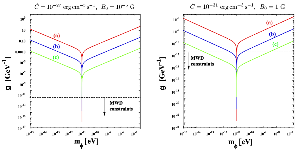
Figure 1: The coupling constant $g$ versus the axion mass $m_{\phi}$ for $\dot{Q}$ equivalent to the two cooling rates $\dot{C}=10^{-27}$ erg cm^-3 s^-1 (left) and $\dot{C}=10^{-31}$ erg cm^-3 s^-1 (right). In the left and right panels, we choose the background magnetic field strength to be $B_{0}=10^{-5}$ G and $B_{0}=1$ G, respectively, with $\omega_{p}=10^{-11}$ eV and $\rho_{\rm DM}=0.3\,{\rm GeV}$ cm^-3 in both cases. The thick colored lines correspond to (a) $\nu=10^{-13}\omega_{p}$, (b) $\nu=10^{-9}\omega_{p}$, and (c) $\nu=10^{-5}\omega_{p}$, respectively. For decreasing $\nu$, the sharper resonance occurs with smaller minimum values of $g$. The dashed black lines represent the observational bound $g\leq 5.4\times 10^{-12}$ GeV^-1 derived from polarization measurements of the MWD stars for the axion mass range $m_{\phi}\leq 3\times 10^{-7}$ eV [35].

For the axion mass $m_{\phi}$ away from the plasma frequency $\omega_{p}$, the resonance does not occur efficiently. In this regime, the bound $\dot{Q}\leq\dot{C}$ translates to $g\leq g_{\rm max}$, where

$$g_{\rm max}=\frac{1}{B_{0}}\sqrt{\frac{\omega_{p}\dot{C}}{\rho_{\rm DM}}}\sqrt{\frac{(r_{\phi}^{2}-1)^{2}+r_{\phi}^{2}r_{\nu}^{2}}{r_{\nu}(r_{\phi}^{2}+r_{\nu}^{2})}}\,,$$ (59)

where

$$r_{\phi}\equiv\frac{m_{\phi}}{\omega_{p}}\,,\qquad r_{\nu}\equiv\frac{\nu}{\omega_{p}}\,.$$ (60)

Let us consider the case in which the inequalities $\nu\ll\omega_{p}$ and $\nu\ll m_{\phi}$ hold, i.e., $r_{\nu}\ll 1$ and $r_{\nu}\ll r_{\phi}$. At the resonance point ($r_{\phi}=1$) and the two asymptotic regimes $r_{\phi}\ll 1$ and $r_{\phi}\gg 1$, respectively, Eq. (59) has the following dependence

$$g_{\rm max} \simeq \frac{1}{B_{0}}\sqrt{\frac{\nu\dot{C}}{\rho_{\rm DM}}}\,,\qquad{\rm for}\quad m_{\phi}=\omega_{p}\,,$$ (61)

$$g_{\rm max} \simeq \frac{\omega_{p}^{2}}{B_{0}m_{\phi}}\sqrt{\frac{\dot{C}}{\rho_{\rm DM}\nu}}\,,\qquad{\rm for}\quad m_{\phi}\ll\omega_{p}\,,$$ (62)

$$g_{\rm max} \simeq \frac{m_{\phi}}{B_{0}}\sqrt{\frac{\dot{C}}{\rho_{\rm DM}\nu}}\,,\qquad{\rm for}\quad m_{\phi}\gg\omega_{p}\,,$$ (63)

where $g_{\rm max}$ in Eq. (61) coincides with the right-hand side of Eq. (58). In the light mass range $m_{\phi}\ll\omega_{p}$, the estimation (62) shows that $g_{\rm max}$ increases with the decrease of $m_{\phi}$. In the heavy mass range $m_{\phi}\gg\omega_{p}$, from Eq. (63), $g_{\rm max}$ grows with the increase of $m_{\phi}$. In these two asymptotic regimes, for smaller $\nu$, we have larger values of $g_{\rm max}$. At the resonance point, $g_{\rm max}$ gets smaller for decreasing $\nu$. These properties are attributed to the fact that the resonance tends to be sharper for smaller $\nu$.

In Fig. 1, we plot $g_{\rm max}$ versus $m_{\phi}$ for three different values of $\nu$. We choose two combinations of $\dot{C}$ and $B_{0}$ in the left and right panels. In both panels, the plasma frequency and the dark matter density are fixed to be $\omega_{p}=10^{-11}$ eV and $\rho_{\rm DM}=0.3\,{\rm GeV}$ cm^-3. For a given $\nu$, $g_{\rm max}$ has a minimum at the resonance mass $m_{\phi}=\omega_{p}$. For decreasing $\nu$, the minimum values of $g_{\rm max}$ get smaller as expected. In both the two asymptotic mass regions $m_{\phi}\ll\omega_{p}$ and $m_{\phi}\gg\omega_{p}$, we can confirm that $g_{\rm max}$ tends to increase for smaller $\nu$.

Since the ratio $r_{\nu}=\nu/\omega_{p}$ of interstellar media given in Table 1 is in the region $10^{-13}\lesssim r_{\nu}\lesssim 10^{-5}$, we have chosen three different values of $\nu$ in this range in Fig. 1. In the left panel, which corresponds to $\dot{C}=10^{-27}$ erg cm^-3 s^-1 and $B_{0}=10^{-5}$ G, we obtain $g_{\rm max}=1.9\times 10^{-16}$ GeV^-1 for the resonance mass $m_{\phi}=\omega_{p}$ with $r_{\nu}=10^{-13}$ [case (a)]. For $r_{\nu}=10^{-9}$ [case (b)] and $r_{\nu}=10^{-5}$ [case (c)], we have $g_{\rm max}=1.9\times 10^{-14}$ GeV^-1 and $g_{\rm max}=1.9\times 10^{-12}$ GeV^-1, respectively. As we observe in the left panel of Fig. 1, the upper limits of $g_{\rm max}$ for these three cases are tighter than the observational bound derived from polarization measurements of the MWD stars. Away from the resonance axion mass, however, the values of $g_{\rm max}$ are much larger than those obtained at $m_{\phi}=\omega_{p}$. For the choices of $\dot{C}$ and $B_{0}$ given in the left panel of Fig. 1, the upper limits of $g_{\rm max}$ derived in the mass ranges $m_{\phi}\ll\omega_{p}$ and $m_{\phi}\gg\omega_{p}$ are much weaker than those computed at $m_{\phi}=\omega_{p}$.

If we were to obtain tighter observational bounds on $\dot{C}$, Eq. (59) shows that $g_{\rm max}$ gets smaller for any mass $m_{\phi}$. This property also holds for $B_{0}$, where the observational finding of interstellar media with $B_{0}$ larger than $10^{-5}$ G results in smaller values of $g_{\rm max}$. In the right panel of Fig. 1, we show $g_{\rm max}$ versus $m_{\phi}$ for $\dot{C}=10^{-31}$ erg cm^-3 s^-1 and $B_{0}=1$ G. As we see in Eq. (59), the coupling $g_{\rm max}$ for given $m_{\phi}$ and $\nu$ is $10^{-7}$ times as small as the one in the left panel. As a result, even the mass range outside the resonance point can enter the parameter space constrained by the MWD measurements. This tendency is more significant for increasing values of $\nu$, even if $g_{\rm max}$ at $m_{\phi}=\omega_{p}$ gets larger. In case (c), for example, the mass range satisfying the bound $g\leq 5.4\times 10^{-12}$ GeV^-1 corresponds to $3.5\times 10^{-14}~{\rm eV}\leq m_{\phi}\leq 2.8\times 10^{-9}~{\rm eV}$. Thus, for smaller $\dot{C}$ and larger $B_{0}$, it is possible to obtain tighter constraints on $g_{\rm max}$ with wider parameter spaces of $m_{\phi}$.

While the data of $\dot{C}$ shown in Table 1 correspond to those of the typical interstellar media, there may be possibilities to find some data of particular regions in the Milky Way galaxy or dwarf galaxies which result in tighter limits on $\dot{C}$ with larger $B_{0}$. We also note that the plasma frequency $\omega_{p}$ can vary for a wider range than those given in Table 1 ($10^{-12}~{\rm eV}\lesssim m_{\phi}\lesssim 10^{-10}~{\rm eV}$). Then, we may be able to obtain more stringent constraints on $g_{\rm max}$ with the wider region of $m_{\phi}$ in future observations.

V Conclusions

In this paper, we proposed a new method of probing the axion-photon coupling through the heating of plasmas in interstellar media. We assumed the presence of an interstellar magnetic field aligned in a particular direction, whose typical value is in the range $B_{0}=10^{-5}~{\rm G}\sim 10^{-3}$ G. We also considered a nonrelativistic thermalized plasma of electrons and heavy ions. The observed cooling rate of interstellar media $\dot{C}$ as well as the electron number density $n_{e}$ and the thermal temperature $T$ are given in Table 1. The latter two data can translate to the plasma frequency $\omega_{p}$ and the friction constant $\nu$, all of which satisfy the condition $\omega_{p}\gg\nu$ with $10^{-12}~{\rm eV}\lesssim\omega_{p}\lesssim 10^{-10}~{\rm eV}$. Although the precise values of $B_{0}$ have been unknown for the data shown in Table 1, we performed forecast constraints on the axion-photon coupling constant $g$ in preparation for upcoming observations of the interstellar plasma.

In Sec. III, we derived solutions to the electric field ${\bm{E}}$ and the vector potential ${\bm{A}}$ by dealing with the axion as nonrelativistic dark matter that oscillates around the potential minimum. We exploited the approximation that spatial gradient terms in the axion and electromagnetic field equations of motion can be neglected relative to time-dependent terms. In the $x$-direction parallel to the external magnetic field ${\bm{B}}_{0}$, we obtained analytic solutions to the $x$ components of ${\bm{E}}$ and ${\bm{A}}$. We showed that both $E_{x}$ and $A_{x}$ are subject to forced resonance, with their leading-order solutions (46) and (44), respectively. In particular, the amplitude ${\cal D}$ in $A_{x}$ has a sharp peak around the resonance axion mass $m_{\phi}=\omega_{p}$. We also found that the axion-photon coupling does not affect the dynamics in the $(y,z)$ plane.

In Sec. IV, we showed that the axion-photon coupling leads to the heating of interstellar media through the resonant energy conversion from axions to photons. In the direction parallel to the external magnetic field, the heating rate $\dot{Q}$ balances the energy damping rate $\dot{Q}_{\nu}$, which represents the energy release from photons to the plasma induced by the friction $\nu$. Since $\dot{Q}$ should not exceed the observed cooling rates $\dot{C}$ of interstellar media, it is possible to put upper bounds on the axion-photon coupling $g$. At the resonance point, $g$ is constrained as Eq. (58). For the typical interstellar magnetic field strength $B_{0}=10^{-5}$ G, we found that $g_{\rm max}$ at the resonance point ($m_{\phi}=\omega_{p}$) can be more stringent than the limit constrained by the MWD measurements. As we see in the left panel of Fig. 1, which corresponds to $B_{0}=10^{-5}$ G and $\dot{C}=10^{-27}$ erg cm^-3 s^-1, $g_{\rm max}$ is much larger than the MWD bound for $m_{\phi}$ away from $\omega_{p}$. However, for larger $B_{0}$ and smaller $\dot{C}$, even the mass range outside the resonance point can enter the region constrained by the MWD measurements. This behavior is clearly seen in the right panel of Fig. 1.

We have thus shown that observations of the interstellar magnetic field along with the cooling rates of plasmas will offer an interesting possibility for constraining the axion-photon coupling $g$. Since the resonance is most efficient for $m_{\phi}$ around $\omega_{p}$ that ranges between $10^{-12}$ eV and $10^{-10}$ eV, we may be able to obtain new bounds on $g$ for the mass region like $10^{-15}~{\rm eV}\lesssim m_{\phi}\lesssim 10^{-7}~{\rm eV}$ with upcoming data. This will bring a new perspective for scrutinizing the properties of light axions as a candidate for dark matter.

Appendix I: Backreaction of electromagnetic fields

We estimate the typical amplitude of the electric field ${\bm{E}}$ in the thermal plasma with temperature $T$. We ignore the contribution of the background magnetic field ${\bm{B}}$ for the moment and exploit the electric-field solution (27) for the time scale $t\lesssim 1/\nu$ (during which ${\bm{E}}$ is not damped by the friction $\nu$). So long as $\omega_{p}\gg\nu$, we have $\dot{{\bm{J}}}\simeq\omega_{p}^{2}{\bm{E}}\simeq\omega_{p}^{2}{\bm{E}}_{0}\cos(\omega_{p}t+\alpha_{0})$ from Eq. (6). This is integrated to give ${\bm{J}}\simeq\omega_{p}{\bm{E}}_{0}\sin(\omega_{p}t+\alpha_{0})$, so that the averaged value of $|{\bm{J}}|^{2}$ over the oscillating period $2\pi/\omega_{p}$ yields $|{\bm{J}}|^{2}\simeq\omega_{p}^{2}E_{0}^{2}/2$, where $E_{0}=|{\bm{E}}_{0}|$. Since ${\bm{J}}=-n_{e}e{\bm{u}}_{e}$, it follows that

$$E_{0}^{2}\simeq\frac{2n_{e}^{2}e^{2}|{\bm{u}}_{e}|^{2}}{\omega_{p}^{2}}=2n_{e}m_{e}|{\bm{u}}_{e}|^{2}\,.$$ (64)

Using the typical thermal electron velocity $|{\bm{u}}_{e}|=\sqrt{2T/m_{e}}$, we have

$$E_{0}\simeq 2\sqrt{n_{e}T}\simeq 5.1\times 10^{-8}\,{\rm eV}^{2}\left(\frac{n_{e}}{0.1\,{\rm cm}^{-3}}\right)^{1/2}\left(\frac{T}{10^{4}\,{\rm K}}\right)^{1/2}\,.$$ (65)

The background magnetic field of order $10^{-5}$ G corresponds to $B_{0}=1.95\times 10^{-7}$ eV². For $n_{e}\approx 0.1\,{\rm cm}^{-3}$ and $T\approx 10^{4}$ K, $E_{0}$ is of a similar order to $B_{0}\approx 10^{-5}$ G.

Let us confirm the validity of the approximation (17). Since the axion amplitude $\bar{\phi}_{0}$ is related to the dark matter density as $\rho_{\rm DM}=m_{\phi}^{2}\bar{\phi}_{0}^{2}/2$, the condition $gE_{0}B_{0}\ll m_{\phi}^{2}\bar{\phi}_{0}$ translates to

$$g\ll 2.1\times 10^{9}\,{\rm GeV}^{-1}\left(\frac{m_{\phi}}{10^{-11}\,{\rm eV}}\right)\left(\frac{B_{0}}{10^{-5}\,{\rm G}}\right)^{-1}\left(\frac{\rho_{\rm DM}}{0.3~{\rm GeV\,cm}^{-3}}\right)^{1/2}\left(\frac{n_{e}}{0.1~{\rm cm}^{-3}}\right)^{-1/2}\left(\frac{T}{10^{4}~{\rm K}}\right)^{-1/2}\,.$$ (66)

For the coupling $g$ constrained in the range (58), the inequality (66) is well satisfied. This is also the case for $g_{\rm max}$ plotted in Fig. 1. Thus, we can trust the homogenous solution (19) of the axion field used in our analysis.

Appendix II: Solutions in the $(y,z)$ plane

Here, we derive the solutions in the $(y,z)$ plane to Eqs. (30), (31), (33), and (34). For this purpose, we will consider the case in which the plasma frequency is much larger than the cyclotron frequency, i.e., $\omega_{p}\gg\omega_{c}$. On using the approximations $|k^{2}A_{y}|\ll|\ddot{A}_{y}|$ and $|k^{2}A_{z}|\ll|\ddot{A}_{z}|$ under the condition (23), we have $J_{y}\simeq\ddot{A}_{y}\simeq-\dot{E}_{y}$ and $J_{z}\simeq\ddot{A}_{z}\simeq-\dot{E}_{z}$ from Eqs. (30) and (31). Substituting these relations into Eqs. (33) and (34), it follows that

$$\ddot{E}_{y}+\nu\dot{E}_{y}+\omega_{p}^{2}E_{y}\simeq-\omega_{c}\dot{E}_{z}\,,$$ (67)

$$\ddot{E}_{z}+\nu\dot{E}_{z}+\omega_{p}^{2}E_{z}\simeq\omega_{c}\dot{E}_{y}\,.$$ (68)

In comparison to Eq. (26), the presence of the magnetic field ${\bm{B}}_{0}$ gives rise to terms proportional to $\omega_{c}$ associated with the quasi-circular motion in the $(y,z)$ plane. Combing Eq. (67) with Eq. (68), we obtain the following fourth-order differential equations

$$\ddddot{E_{i}}+2\nu\dddot{E_{i}}+\left(2\omega_{p}^{2}+\omega_{c}^{2}+\nu^{2}\right)\ddot{E_{i}}+2\nu\omega_{p}^{2}\dot{E_{i}}+\omega_{p}^{4}E_{i}=0\,,$$ (69)

for both $i=y,z$. Assuming the solutions to these equations in the form $E_{i}=E_{i0}e^{\lambda t}$, where $E_{i0}$ and $\lambda$ are constants, we obtain the algebraic equation

$$\left(\lambda^{2}+\nu\lambda+\omega_{p}^{2}\right)^{2}+\omega_{c}^{2}\lambda^{2}=0\,.$$ (70)

For $\omega_{c}=0$, the solution is given by $\lambda=(-\nu\pm\sqrt{\nu^{2}-4\omega_{p}^{2}})/2$, which reduces to $\lambda\simeq-\nu/2\pm i\omega_{p}$ under the approximation $\omega_{p}\gg\nu$. For $\omega_{c}\neq 0$ with $\omega_{p}\gg\omega_{c}$, we assume the solution to Eq. (70) in the form $\lambda=-\nu/2\pm i\omega_{p}+\epsilon$, where $|\epsilon|\ll\omega_{p}$. Substituting this into Eq. (70) and picking up the dominant contribution to $\epsilon$, it follows that

$$\lambda\simeq-\frac{\nu}{2}\pm i\omega_{p}\pm\frac{i}{2}\omega_{c}\,,$$ (71)

which is valid for $\omega_{p}\gg\nu$ and $\omega_{p}\gg\omega_{c}$. Depending on the different signs in Eq. (71), we have four independent solutions to Eq. (70). Thus, the general solution to $E_{y}$ can be expressed as

$$E_{y}\simeq e^{-\nu t/2}\left[c_{1}\cos\left\{\left(\omega_{p}+\frac{\omega_{c}}{2}\right)t+\alpha_{1}\right\}+c_{2}\cos\left\{\left(\omega_{p}-\frac{\omega_{c}}{2}\right)t+\alpha_{2}\right\}\right]\,,$$ (72)

where $c_{1},c_{2},\alpha_{1},\alpha_{2}$ are constants. From Eq. (67), the other electric-field component $E_{z}$ is related to $E_{y}$. Dropping the contribution to $E_{z}$ from $\nu$ except the damping factor $e^{-\nu t/2}$ and using the approximation $\omega_{p}\gg\omega_{c}\neq 0$, we find

$$E_{z}\simeq e^{-\nu t/2}\left[c_{1}\left(1-\frac{\omega_{c}}{4\omega_{p}}\right)\sin\left\{\left(\omega_{p}+\frac{\omega_{c}}{2}\right)t+\alpha_{1}\right\}-c_{2}\left(1+\frac{\omega_{c}}{4\omega_{p}}\right)\sin\left\{\left(\omega_{p}-\frac{\omega_{c}}{2}\right)t+\alpha_{2}\right\}\right]\,.$$ (73)

In both $E_{y}$ and $E_{z}$ components, there are two oscillating modes characterized by the frequencies $\omega_{p}\pm\omega_{c}/2$. So long as $\omega_{p}\gg\omega_{c}$, they are dominated by the plasma frequency with the oscillating time scale $t_{p}\approx 1/\omega_{p}$. For $\omega_{p}\gg\nu$, $t_{p}$ is much shorter than the damping time scale $t_{d}\approx 1/\nu$ induced by the friction term. When $\omega_{c}\neq 0$, the phases of oscillating terms in $E_{y}$ and $E_{z}$ are correlated with each other. If the initial conditions of $E_{y}$ and $E_{z}$ are chosen to be $c_{2}=0$, for example, we have $E_{y}^{2}/a^{2}+E_{z}^{2}/b^{2}=1$, where $a=c_{1}e^{-\lambda t/2}$ and $b=c_{1}[1-\omega_{c}/(4\omega_{p})]e^{-\lambda t/2}$. This corresponds to the ellipse where the major radius $a$ and the minor radius $b$ decrease with the time scale $t_{d}$. As we observe in Eqs. (30)-(31) and (33)-(34), the coupling between axions and photons does not appear in the dynamics in the ($y,z$) plane and hence the electric field component $E_{y}$ or $E_{z}$ is not enhanced. While the above solutions to $E_{y}$ and $E_{z}$ have been derived under the condition $\omega_{p}\gg\omega_{c}$, the absence of energy transfer from axions to photons in the ($y,z$) plane persists for general values of $\omega_{p}$ and $\omega_{c}$.

References

- Peccei and Quinn [1977] R. D. Peccei and H. R. Quinn, Phys. Rev. Lett. 38, 1440 (1977).
- Weinberg [1978] S. Weinberg, Phys. Rev. Lett. 40, 223 (1978).
- Wilczek [1978] F. Wilczek, Phys. Rev. Lett. 40, 279 (1978).
- Grilli di Cortona et al. [2016] G. Grilli di Cortona, E. Hardy, J. Pardo Vega, and G. Villadoro, JHEP 01, 034 (2016), arXiv:1511.02867 [hep-ph] .
- Kim [1979] J. E. Kim, Phys. Rev. Lett. 43, 103 (1979).
- Shifman et al. [1980] M. A. Shifman, A. I. Vainshtein, and V. I. Zakharov, Nucl. Phys. B 166, 493 (1980).
- Dine et al. [1981] M. Dine, W. Fischler, and M. Srednicki, Phys. Lett. B 104, 199 (1981).
- Zhitnitsky [1980] A. R. Zhitnitsky, Sov. J. Nucl. Phys. 31, 260 (1980).
- Preskill et al. [1983] J. Preskill, M. B. Wise, and F. Wilczek, Phys. Lett. B 120, 127 (1983).
- Abbott and Sikivie [1983] L. F. Abbott and P. Sikivie, Phys. Lett. B 120, 133 (1983).
- Dine and Fischler [1983] M. Dine and W. Fischler, Phys. Lett. B 120, 137 (1983).
- Kim [1987] J. E. Kim, Phys. Rept. 150, 1 (1987).
- Raffelt [1990] G. G. Raffelt, Phys. Rept. 198, 1 (1990).
- Kim and Carosi [2010] J. E. Kim and G. Carosi, Rev. Mod. Phys. 82, 557 (2010), [Erratum: Rev.Mod.Phys. 91, 049902 (2019)], arXiv:0807.3125 [hep-ph] .
- Marsh [2016] D. J. E. Marsh, Phys. Rept. 643, 1 (2016), arXiv:1510.07633 [astro-ph.CO] .
- Di Luzio et al. [2020] L. Di Luzio, M. Giannotti, E. Nardi, and L. Visinelli, Phys. Rept. 870, 1 (2020), arXiv:2003.01100 [hep-ph] .
- Kim et al. [2014] J. E. Kim, Y. Semertzidis, and S. Tsujikawa, Front. in Phys. 2, 60 (2014), arXiv:1409.2497 [hep-ph] .
- Witten [1984] E. Witten, Phys. Lett. B 149, 351 (1984).
- Svrcek and Witten [2006] P. Svrcek and E. Witten, JHEP 06, 051 (2006), arXiv:hep-th/0605206 .
- Conlon [2006] J. P. Conlon, JHEP 05, 078 (2006), arXiv:hep-th/0602233 .
- Arvanitaki et al. [2010] A. Arvanitaki, S. Dimopoulos, S. Dubovsky, N. Kaloper, and J. March-Russell, Phys. Rev. D 81, 123530 (2010), arXiv:0905.4720 [hep-th] .
- Acharya et al. [2010] B. S. Acharya, K. Bobkov, and P. Kumar, JHEP 11, 105 (2010), arXiv:1004.5138 [hep-th] .
- Cicoli et al. [2012] M. Cicoli, M. Goodsell, and A. Ringwald, JHEP 10, 146 (2012), arXiv:1206.0819 [hep-th] .
- Halverson et al. [2017] J. Halverson, C. Long, and P. Nath, Phys. Rev. D 96, 056025 (2017), arXiv:1703.07779 [hep-ph] .
- Demirtas et al. [2020] M. Demirtas, C. Long, L. McAllister, and M. Stillman, JHEP 04, 138 (2020), arXiv:1808.01282 [hep-th] .
- Sikivie [1983] P. Sikivie, Phys. Rev. Lett. 51, 1415 (1983), [Erratum: Phys.Rev.Lett. 52, 695 (1984)].
- Ehret et al. [2009] K. Ehret et al. (ALPS), Nucl. Instrum. Meth. A 612, 83 (2009), arXiv:0905.4159 [physics.ins-det] .
- Ehret et al. [2010] K. Ehret et al., Phys. Lett. B 689, 149 (2010), arXiv:1004.1313 [hep-ex] .
- Anastassopoulos et al. [2017] V. Anastassopoulos et al. (CAST), Nature Phys. 13, 584 (2017), arXiv:1705.02290 [hep-ex] .
- Armengaud et al. [2014] E. Armengaud et al., JINST 9, T05002 (2014), arXiv:1401.3233 [physics.ins-det] .
- Primakoff [1951] H. Primakoff, Phys. Rev. 81, 899 (1951).
- Raffelt [1986] G. G. Raffelt, Phys. Rev. D 33, 897 (1986).
- Payez et al. [2015] A. Payez, C. Evoli, T. Fischer, M. Giannotti, A. Mirizzi, and A. Ringwald, JCAP 02, 006 (2015), arXiv:1410.3747 [astro-ph.HE] .
- Dessert et al. [2020] C. Dessert, J. W. Foster, and B. R. Safdi, Phys. Rev. Lett. 125, 261102 (2020), arXiv:2008.03305 [hep-ph] .
- Dessert et al. [2022] C. Dessert, D. Dunsky, and B. R. Safdi, Phys. Rev. D 105, 103034 (2022), arXiv:2203.04319 [hep-ph] .
- Hu et al. [2000] W. Hu, R. Barkana, and A. Gruzinov, Phys. Rev. Lett. 85, 1158 (2000), arXiv:astro-ph/0003365 .
- Fujita et al. [2019] T. Fujita, R. Tazaki, and K. Toma, Phys. Rev. Lett. 122, 191101 (2019), arXiv:1811.03525 [astro-ph.CO] .
- Adachi et al. [2023] S. Adachi et al. (POLARBEAR), Phys. Rev. D 108, 043017 (2023), arXiv:2303.08410 [astro-ph.CO] .
- Xue et al. [2024] X. Xue et al., arXiv:2412.02229 [astro-ph.HE] .
- Fedderke et al. [2019] M. A. Fedderke, P. W. Graham, and S. Rajendran, Phys. Rev. D 100, 015040 (2019), arXiv:1903.02666 [astro-ph.CO] .
- Minami and Komatsu [2020] Y. Minami and E. Komatsu, Phys. Rev. Lett. 125, 221301 (2020), arXiv:2011.11254 [astro-ph.CO] .
- Diego-Palazuelos et al. [2022] P. Diego-Palazuelos et al., Phys. Rev. Lett. 128, 091302 (2022), arXiv:2201.07682 [astro-ph.CO] .
- Carroll [1998] S. M. Carroll, Phys. Rev. Lett. 81, 3067 (1998), arXiv:astro-ph/9806099 .
- Lue et al. [1999] A. Lue, L.-M. Wang, and M. Kamionkowski, Phys. Rev. Lett. 83, 1506 (1999), arXiv:astro-ph/9812088 .
- Fujita et al. [2021a] T. Fujita, Y. Minami, K. Murai, and H. Nakatsuka, Phys. Rev. D 103, 063508 (2021a), arXiv:2008.02473 [astro-ph.CO] .
- Fujita et al. [2021b] T. Fujita, K. Murai, H. Nakatsuka, and S. Tsujikawa, Phys. Rev. D 103, 043509 (2021b), arXiv:2011.11894 [astro-ph.CO] .
- [47] F. Chen, Introduction to Plasma Physics and Controlled Fusion, Springer International Publishing (2016).
- Gibbon [2027] P. Gibbon, arXiv:1705.10529 [physics.acc-ph] .
- Ferriere [2009] K. Ferriere, Astron. Astrophys. 505, 1183 (2009), arXiv:0908.2037 [astro-ph.GA] .
- Matsuhara et al. [1997] H. Matsuhara, M. Tanaka, Y. Yonekura, Y. Fukui, M. Kawada, and J. J. Bock, Astrophys. J. 490, 744 (1997), arXiv:astro-ph/9707264 .
- Lehner et al. [2004] N. Lehner, B. P. Wakker, and B. D. Savage, Astrophys. J. 615, 767 (2004), arXiv:astro-ph/0407363 .
- Wadekar and Farrar [2021] D. Wadekar and G. R. Farrar, Phys. Rev. D 103, 123028 (2021), arXiv:1903.12190 [hep-ph] .
- Wadekar and Wang [2023] D. Wadekar and Z. Wang, Phys. Rev. D 107, 083011 (2023), arXiv:2211.07668 [hep-ph] .
- Chivukula et al. [1990] R. S. Chivukula, A. G. Cohen, S. Dimopoulos, and T. P. Walker, Phys. Rev. Lett. 65, 957 (1990).
- Dubovsky and Hernández-Chifflet [2015] S. Dubovsky and G. Hernández-Chifflet, JCAP 12, 054 (2015), arXiv:1509.00039 [hep-ph] .
- Hardy and Lasenby [2017] E. Hardy and R. Lasenby, JHEP 02, 033 (2017), arXiv:1611.05852 [hep-ph] .
- Bhoonah et al. [2018] A. Bhoonah, J. Bramante, F. Elahi, and S. Schon, Phys. Rev. Lett. 121, 131101 (2018), arXiv:1806.06857 [hep-ph] .
- Bhoonah et al. [2019] A. Bhoonah, J. Bramante, F. Elahi, and S. Schon, Phys. Rev. D 100, 023001 (2019), arXiv:1812.10919 [hep-ph] .
- Farrar et al. [2020] G. R. Farrar, F. J. Lockman, N. M. McClure-Griffiths, and D. Wadekar, Phys. Rev. Lett. 124, 029001 (2020), arXiv:1903.12191 [hep-ph] .
- Bhoonah et al. [2021] A. Bhoonah, J. Bramante, S. Schon, and N. Song, Phys. Rev. D 103, 123026 (2021), arXiv:2010.07240 [hep-ph] .
- Wadekar and Wang [2022] D. Wadekar and Z. Wang, Phys. Rev. D 106, 075007 (2022), arXiv:2111.08025 [hep-ph] .
- Shoji et al. [2024] Y. Shoji, E. Kuflik, Y. Birnboim, and N. C. Stone, Mon. Not. Roy. Astron. Soc. 528, 4082 (2024), arXiv:2306.08679 [astro-ph.CO] .
- Takeshita and Kitabayashi [2024] A. Takeshita and T. Kitabayashi, arXiv:2409.03981 [hep-ph] .