The galaxy UV luminosity function from the JWST Advanced Deep Extragalactic Survey: insights into early galaxy evolution and reionization
Abstract
The high-redshift UV luminosity function provides important insights into the evolution of early galaxies. JWST has revealed an unexpectedly large population of bright () galaxies at , implying fundamental changes in the star forming properties of galaxies at increasingly early times. However, constraining the fainter population () has been more challenging. In this work, we present the UV luminosity function from the JWST Advanced Deep Extragalactic Survey. We calculate the UV luminosity function from several hundred galaxy candidates that reach UV luminosities of in redshift bins of (309 candidates) and (63 candidates). We search for candidates at and find none. We also estimate the luminosity function from the subset of the sample. Consistent with other measurements, we find an excess of bright galaxies that is in tension with many theoretical models, especially at . However, we also find high number densities at , suggesting that there is a larger population of faint galaxies than expected, as well as bright ones. From our parametric fits for the luminosity function, we find steep faint end slopes of , suggesting a large population of faint () galaxies. Combined, the high normalization and steep faint end slope of the luminosity function could imply that the reionization process is appreciably underway as early as .
1 Introduction
The formation and evolution of galaxies within the first few hundred million years after the Big Bang played an essential part in shaping the evolution of the Universe. The emergence of these early galaxies marks the transition from a nearly homogeneous Universe composed primarily of neutral hydrogen to one filled with galaxies hosted in large scale dark matter overdensities, all embedded in an ionized intergalactic medium (IGM). Moreover, there is substantial evidence that galaxies were not only present for this key phase transition of the Universe from neutral to ionized hydrogen – called cosmic reionization – but that they were capable of providing most of the photons responsible for reionizing the Universe (for a recent review, see Robertson, 2022). Thus, observing galaxies at these early times provides crucial insights into the early phases of star formation and the process of hydrogen reionization.
The identification and characterization of galaxies within a billion years after the Big Bang was first enabled by near-infrared ( m) observations with the Hubble Space Telescope (HST) and ground-based facilities. Together, these data enabled thousands of star-forming galaxies at ( Myr after the Big Bang) and tens at ( Myr after the Big Bang) to be identified (e.g. Stanway et al. 2003; Bunker et al. 2004, 2010; Ellis et al. 2013; McLure et al. 2013; Finkelstein et al. 2015, 2022a; McLeod et al. 2016; Bouwens et al. 2021; also see Stark 2016 for a review) spanning more than four orders of magnitude in rest-frame ultraviolet (UV) continuum luminosities. This allowed the high-redshift rest-UV luminosity function to be measured at luminosities as bright as and as faint as (e.g. Bouwens et al., 2011, 2015, 2021; Bowler et al., 2014, 2015, 2020; Finkelstein et al., 2015, 2022a; McLeod et al., 2016; Livermore et al., 2017; Oesch et al., 2018; Rojas-Ruiz et al., 2020). At the faint end of the luminosity function, primarily accessible with space-based observations, these studies revealed steep faint end slopes of (implying that faint, objects dominated galaxy number counts during reionization), while ground-based studies found evidence of an increase in the number of very bright () galaxies at compared to lower redshifts (i.e. a change in the shape of the bright end of the luminosity function, suggesting a redshift evolution of the physical processes impacting the UV luminosity of galaxies). However, the limited near-infrared wavelength coverage of HST made it extremely challenging to robustly perform rest-UV photometric selections at .
With JWST (Gardner et al., 2006, 2023), our understanding of galaxies within the first Myr after the Big Bang has changed significantly over the last few years. Photometric selections using early JWST/Near Infrared Camera (NIRCam; Rieke et al., 2005, 2023a) imaging quickly identified large numbers of galaxy candidates (e.g. Naidu et al., 2022; Castellano et al., 2022; Adams et al., 2023; Donnan et al., 2023; Harikane et al., 2023; Finkelstein et al., 2023; Whitler et al., 2023; Robertson et al., 2023; Hainline et al., 2024a). Subsequent spectroscopic observations with the JWST/Near Infrared Spectrograph (NIRSpec; Jakobsen et al., 2022; Ferruit et al., 2022) have now unequivocally confirmed the existence of many galaxies up to redshifts as high as (e.g. Curtis-Lake et al., 2023; Fujimoto et al., 2023; Arrabal Haro et al., 2023; Wang et al., 2023; Castellano et al., 2024; D’Eugenio et al., 2024a; Carniani et al., 2024a; Napolitano et al., 2024a), many of which are bright in the rest-frame UV (; e.g. Finkelstein et al., 2022b; Castellano et al., 2024; Carniani et al., 2024a; Napolitano et al., 2024a). Given the rarity of similarly bright, early galaxies predicted by existing theoretical galaxy evolution models (e.g. Yung et al., 2019; Behroozi et al., 2020; Rosdahl et al., 2022; Wilkins et al., 2023), the discovery of these bright galaxies in moderately small survey areas tentatively suggested that such systems were unexpectedly abundant in the early Universe.
Over time and with the maturation of JWST, insights into the galaxy population as a whole have become accessible. Consistent with the large number of bright galaxies implied by individual discoveries, JWST measurements of the rest-UV luminosity function at have typically found only a slow decline in the number densities of galaxies (e.g. Adams et al. 2023; Bouwens et al. 2023; Castellano et al. 2023; Donnan et al. 2023, 2024; Harikane et al. 2023, 2024a, 2024b; McLeod et al. 2024; Finkelstein et al. 2024, though Willott et al. 2024 found a faster evolution that could be attributed to field-to-field variance). This slow evolutionary trend is a significant departure from many theoretical expectations established prior to JWST, prompting many potential explanations to be explored theoretically. For example, the efficiency of star formation may be higher than previously predicted at high redshift (e.g. Dekel et al., 2023; Li et al., 2024; Harikane et al., 2023; Ceverino et al., 2024; Feldmann et al., 2025). Star formation may be extremely stochastic or “bursty” at early times (e.g. Mason et al., 2023; Mirocha & Furlanetto, 2023; Shen et al., 2023; Sun et al., 2023; Kravtsov & Belokurov, 2024; Gelli et al., 2024). The stellar initial mass function may be more top-heavy in the early Universe (e.g. Harikane et al. 2023; Yung et al. 2024, though c.f. Cueto et al. 2024). Dust attenuation may decrease at high redshift (e.g. Ferrara et al., 2023; Fiore et al., 2023). Or, there may be a significant population of active galactic nuclei (e.g. Hegde et al., 2024). In particular, bursty star formation has been shown to significantly alleviate the tension between models and observations (e.g. Sun et al., 2023; Kravtsov & Belokurov, 2024; Gelli et al., 2024), which is also consistent with the spectral energy distributions (SEDs) of high-redshift galaxies (e.g. Tacchella et al., 2023; Looser et al., 2023, 2024; Endsley et al., 2023, 2024; Witten et al., 2024; Boyett et al., 2024). However, it is challenging for any single physical mechanism to fully reconcile observations and theoretical predictions and it is likely that a large population of bright galaxies is sustained by a combination of several factors.
Moreover, while much attention has been dedicated to observing and understanding the bright galaxy population, the complete picture of galaxies at all luminosities has been more challenging to characterize. It is now generally agreed that the abundance of galaxies declines relatively slowly at at least until , but these objects do not represent the majority of the overall galaxy population. The steep faint end slopes of UV luminosity functions imply that faint, galaxies dominate galaxy number counts and the total cosmic UV luminosity density at high redshift. Studying only the bright galaxy population provides an incomplete perspective on galaxies in the early Universe; identifying and characterizing fainter galaxies despite the observational challenges is necessary for a holistic understanding of the evolution of high-redshift galaxies and how galaxies contribute to the process of cosmic reionization.
In this work, we aim to place new, direct constraints on the faint end () of the UV luminosity function at using deep JWST/NIRCam imaging taken as part of the JWST Advanced Deep Extragalactic Survey (JADES; Eisenstein et al., 2023a; Rieke et al., 2023b). We take advantage of three dropout filters at m to photometrically select galaxy candidates that lie at and that span nearly a factor of in far-UV continuum ( Å) luminosity. We can select bright, candidates over the full area of the JADES imaging we use in this work ( arcmin2), while candidates are identified in the arcmin2 of the imaging that reaches depths of . This depth is comparable to the JADES Origins Field, or JOF, in which the UV luminosity function has been independently measured (Robertson et al., 2024), as well as the Next Generation Deep Extragalactic Exploratory Public survey (Leung et al., 2023) and the NIRCam parallel to the MIRI Deep Imaging Survey (Pérez-González et al., 2023). Using these deep data from JADES, we can directly constrain the slope of the faint end of the luminosity function, investigate implications for early star formation processes in the context of both the bright and faint galaxy population, and examine the role of galaxies in reionizing the Universe.
This paper is organized as follows. We describe our imaging data, reduction techniques, and photometric measurements in Section 2. We then present our selection methods in Section 3 and discuss the general observed properties of our samples in Section 4. In Section 5, we present our measurement of the rest-UV luminosity function in two bins of redshift spanning and , an upper limit on the UV luminosity function at , and the corresponding redshift evolution of the cosmic UV luminosity density. We then place our results in the context of theoretical galaxy formation models and discuss implications for the reionization timeline in Section 6. Finally, we summarize our key results and conclusions in Section 7.
Throughout this work, we assume a standard flat CDM cosmology with , , and and all magnitudes are given in the AB system (Oke & Gunn, 1983). Unless stated otherwise, all physical lengths are comoving and reported values and uncertainties correspond to the marginalized median, 16, and 84 percentiles.
2 Data and Photometry
| Subregion | Area [arcmin2] | F090W | F115W | F150W | F200W | F277W | F356W | F410M | F444W |
|---|---|---|---|---|---|---|---|---|---|
| s | 33.7 | 28.4 | 28.8 | 28.7 | 28.7 | 29.3 | 29.0 | 27.9 | 29.1 |
| s | 91.9 | 29.2 | 29.5 | 29.5 | 29.6 | 30.0 | 29.9 | 29.3 | 29.6 |
| s | 25.8 | 30.1 | 30.3 | 30.3 | 30.4 | 30.7 | 30.7 | 30.1 | 30.4 |
| s | 12.0 | 30.4 | 30.7 | 30.7 | 30.7 | 31.0 | 31.0 | 30.4 | 30.7 |
| All | 163.5 | 28.9 | 29.3 | 29.3 | 29.3 | 29.8 | 29.6 | 28.6 | 29.5 |
In this work, we use deep near-infrared JWST imaging obtained as part of the JADES program (Eisenstein et al., 2023a), combined with archival HST/Advanced Camera for Surveys (ACS) optical imaging from the Hubble Legacy Fields (HLF) project (Illingworth et al., 2016; Whitaker et al., 2019). We refer to Eisenstein et al. (2023a) and Rieke et al. (2023b) for a full description of the JADES design and dataset but provide a brief summary of the JADES NIRCam data here.
The JADES NIRCam imaging consists of observations in both the North and South fields of the Great Observatories Origins Deep Survey (GOODS-N and GOODS-S; Giavalisco et al., 2004) under program IDs 1180 and 1181 (PI Eisenstein), 1210 and 1286 (PI Luetzgendorf), and 1287 (PI Isaak). JADES observed both fields in eight NIRCam filters over the entire footprint (F090W, F115W, F150W, F200W, F277W, F356W, F410M, and F444W), with the addition of F070W and/or F335M in some regions of the footprint. Additionally, subregions of the JADES NIRCam footprint overlap with imaging taken by other JWST programs, some of which we use when constructing the data products used in this work. Specifically, we include the arcmin2 of F162M, F182M, F210M, F250M, F300M, and F335M imaging in the JADES GOODS-S footprint taken by program ID 3215 (PIs Eisenstein and Maiolino), the area of which comprises the JOF (Eisenstein et al., 2023b). There is also arcmin2 of F182M, F210M, F430M, F460M, and F480M imaging in GOODS-S from the JWST Extragalactic Medium-band Survey (JEMS, program ID 1963; PIs Williams, Tacchella, and Maseda; Williams et al., 2023) and arcmin2 in both GOODS-N and GOODS-S of F182M, F210M, and F444W observations from the First Reionization Epoch Spectroscopically Complete Observations (FRESCO, program ID 1895; Oesch et al., 2023) survey. Data from program 3215, JEMS, and FRESCO are co-reduced with JADES observations and included in the final NIRCam mosaics and photometric catalogs. We refer to Rieke et al. (2023b); Eisenstein et al. (2023a, b), and Tacchella et al. (in prep.) for more detailed descriptions of the NIRCam image reduction and Robertson et al. (in prep.) for the detection and photometry methods, but provide a summary below.
2.1 Images
We process the JADES, JEMS, FRESCO, and program 3215 NIRCam data with version 1.11.4 of the JWST Science Calibration Pipeline (jwst) and Calibration Reference Data System pipeline mapping jwst_1130.pmap, with some custom steps for correction of imaging artifacts, astrometric alignment, and background subtraction. We run jwst Stage 1 to perform detector-level corrections and ramp fitting, largely with the default parameters (with the exception of identifying and correcting “snowball” artifacts from cosmic rays, for which we use custom parameters; Robertson et al., 2024). We then run jwst Stage 2 with the default parameters using sky flats provided by the Space Telescope Science Institute for the short wavelength (SW) filters, F250M, and F300M, and custom super-sky flats for all other long wavelength (LW) filters.
After the completion of Stage 2, we fit and subtract several common additive features seen in NIRCam data (Rigby et al., 2023): noise, artifacts from scattered light111https://jwst-docs.stsci.edu/known-issues-with-jwst-data/nircam-known-issues/nircam-scattered-light-artifacts (Rigby et al., 2023), and a large-scale background. We also perform a custom astrometric alignment to HST images that were registered to Gaia DR2 (Gaia Collaboration et al. 2018; G. Brammer, private communication) using a modified version of the jwst TweakReg package. Finally, for each filter, we combine the individual calibrated exposures into a single mosaic using the default parameters of jwst Stage 3. We set the pixel scale to 0.03″ pixel-1 and choose a drizzle parameter of pixfrac = 1 for both the SW and LW images.
2.2 Detection and Photometry
We run source detection on a signal-to-noise ratio (SNR) image that includes all of the available LW NIRCam mosaics in a given region, at their original resolution (i.e. without PSF homogenization). In GOODS-S, these filters are F250M, F277W, F300M, F335M, F356W, F410M, F430M, F444W, F460M, and F480M. In GOODS-N, the detection image includes F277W, F335M, F356W, F410M, and F444W. To produce the SNR stack, we first median filter the error images of individual filters to remove small-scale features introduced by incomplete masking in the jwst pipeline, then construct the signal and noise images as the inverse variance weighted stack of the science and median filtered error channels for the relevant filters. The final SNR image on which we perform detection is the ratio of these stacks.
To construct the segmentation map, we select initial regions of interest by applying a significance threshold of , then refine the segmentations with a series of custom computational morphology algorithms inspired by NoiseChisel (Akhlaghi & Ichikawa, 2015). Stars and diffraction spikes are masked, the segmentation map is deblended using a logarithmic scaling of the F200W image, then further refined by applying a high-pass filter to the outer regions of large segmentations to identify nearby satellites. Finally, the segmentations of already identified objects are masked out of the detection image and a final search for faint objects that may have previously been missed is performed.
We next use the photutils (Bradley et al., 2023) package to do custom forced aperture photometry on the objects detected as described above. Object centroids are computed as the windowed positions used by Source Extractor (Bertin & Arnouts, 1996) and photometry is measured in several circular apertures () and Kron (1980) elliptical apertures with Kron parameters of and . Kron apertures are determined using the inverse variance weighted signal image stack (the numerator of the detection image) with area limited to be less than twice that of an object’s segmentation area.
To calculate aperture corrections, we produce model point spread functions (mPSFs) following the methods of Ji et al. (2023), wherein the mPSF is measured from mosaics of WebbPSF models that are constructed using the same exposure pattern as the real observations. The aperture correction for a circular aperture of a given size is measured from the mPSF and applied to every source in the catalog in the same way, while the Kron aperture corrections are calculated on a source-by-source basis by placing the appropriate elliptical aperture on the mPSF. Aperture corrections for HST bands are measured from empirical PSFs constructed using visually inspected stars in the field.
Finally, photometric uncertainties are calculated as the quadrature sum of the Poisson noise from a given source and sky noise measured from apertures randomly placed on blank areas of the mosaics that depends on aperture size and exposure time.222The sky noise is measured by randomly placing circular apertures of various sizes in object-free regions of the mosaics, calculating the root-mean-square error of electron counts as a function of aperture size, and interpolating between exposure times and aperture sizes. For the Kron photometry, the circularized radius of the elliptical aperture is used to determine the random aperture contribution to the uncertainty.
| Dropout Sample | Redshift | Criteria |
|---|---|---|
| F115W | in at least four of F150W, F200W, F277W, F356W, F410M, and F444W | |
| in all of F150W, F200W, F277W, F356W, and F444W | ||
| ( in F090W) or () | ||
| ) or () | ||
| F150W | in at least three of F200W, F277W, F356W, F410M, and F444W | |
| in all of F200W, F277W, F356W, and F444W | ||
| ( in F090W and F115W) or (( in one of F090W and F115W) | ||
| and ()) | ||
| () or () | ||
| F200W | in at least three of F277W, F356W, F410M, and F444W | |
| in all of F277W, F356W, and F444W | ||
| ( in F090W, F115W, and F150W) or (( in two of F090W, F115W, | ||
| and F150W) and ()) | ||
| () or () |
The full JADES NIRCam imaging, combined with that from JEMS, FRESCO, and program 3215, comprises a rich dataset, sometimes with up to 14 bands of NIRCam imaging in the same area (Eisenstein et al., 2023b). However, due to the multiple observational programs targeting different areas with different filters for different amounts of time, the imaging is also very complex with heterogeneous filter coverage and depths over the full area. The image used for source detection incorporates all of the LW images available at a given location (Section 2.2), but for simplicity, we otherwise restrict our analysis to the eight NIRCam filters (F090W, F115W, F150W, F200W, F277W, F356W, F410M, and F444W) in which JADES obtained its primary imaging (Eisenstein et al., 2023a). Correspondingly, we only select candidates and calculate the UV luminosity function in the area covered by all eight of these filters, a total of arcmin2 ( arcmin2 in GOODS-S and arcmin2 in GOODS-N).
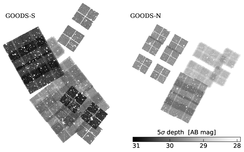
In Table 1, we report the depths for the NIRCam images in this limited area. To measure depths, we mask sources out of the image using the segmentation map, then calculate aperture corrected photometry in blank regions of the field using the circular apertures (named CIRC1 in the JADES photometric catalog) that we use for sample selection (Section 3). We note that the exposure times over the full JADES area can vary by more than a factor of 16 in F200W, leading to upwards of a factor of four difference in depth between the shallowest and deepest regions of the images (). We illustrate this variation in depth in Figure 1, where darker grey indicates deeper imaging. Thus, though we do not explicitly subdivide the full JADES field into subregions while calculating the UV luminosity function, we report the depths in four regimes of F200W exposure time to approximately describe the area of the JADES imaging that constrains the faint end of the luminosity function. The deepest ( s in F200W) arcmin2 area is typically mag deeper than the shallowest ( s) arcmin2 subregion, reaching typical depths of .
3 Sample selection
3.1 Photometric Selection Criteria
With the photometric catalogs in hand, we now turn to selecting high-redshift galaxy candidates. At , the Ly break redshifts progressively through the NIRCam F115W (), F150W (), and F200W () filter. We search for high-redshift galaxy candidates primarily through three sets of color criteria, one for each of these three dropout filters, then apply secondary selection criteria to further clean the samples. We enumerate the exact color cuts in Table 2 but provide a general description below. In brief, our selections are designed to require that high-redshift galaxy candidates satisfy the following:
-
1.
have a red dropout color (, , and greater than 1.3 for the F115W, F150W, and F200W dropout samples, respectively),
-
2.
are robustly detected in the filters expected to probe the rest-frame UV and rest-frame optical ( in all of these filters and in more than half of them),
-
3.
are not detected (signal-to-noise of ) in any of the NIRCam filters blueward of the filter expected to contain the Ly break,
-
4.
do not have an extremely red color in filters expected to probe the rest-frame UV (, , and less than 1.0 for the F115W, F150W, and F200W dropout samples, respectively), and
-
5.
have an increasingly strong Ly break the redder the rest-UV colors are ().
We use photometry measured in circular apertures (i.e. CIRC1) for sample selection, as these apertures have less background noise than larger apertures and most high-redshift galaxies are expected to be comparable in size to the ( proper kpc at ) CIRC1 aperture (e.g. Shibuya et al., 2015; Yang et al., 2022; Ono et al., 2023, 2024; Morishita et al., 2024). We note that we use photometry measured on native resolution mosaics, which may result in bluer colors for our objects of interest than PSF matched images, as the size of the PSF increases with increasing wavelength and our aperture corrections assume point sources (but our objects are likely to be at least marginally resolved). To assess the impact of this effect, we perform source injection and recovery simulations on the same native resolution mosaics (see Section 5.1) and find only a mild systematic bias in photometric colors at wavelengths longer than the Ly break (at most mag). We observe little, if any, bias in the dropout colors, which we attribute to only the red filter having significant amounts of flux that may introduce bias. At longer wavelengths, both filters are expected to be detected and therefore both may introduce bias in the color (e.g. one filter may be underestimated and one may be overestimated).
| Parameter | Description | Prior |
|---|---|---|
| Redshift | Uniform, | |
| Formed stellar mass | Uniform in log, | |
| Stellar metallicity | Uniform in log, | |
| Diffuse dust optical depth in the -band | Uniform in log, | |
| Ionization parameter | Uniform in log, | |
| Maximum stellar age (i.e. onset of star formation) | Uniform in log, | |
| Delayed exponential -folding time | Uniform in log, | |
| Duration of recent constant component | Uniform in log, | |
| sSFR of recent constant component | Uniform in log, |
If the CIRC1 flux for an object has in the dropout filter for each selection, we set the flux to the flux error before applying the selection criteria in Table 2. Additionally, for each of the F150W and F200W dropout candidates, we require that the object is not selected by any of the lower redshift selections (which may happen in the case of partial dropouts). For example, if an F150W dropout is also selected by the F115W dropout selection, we consider the object an F115W dropout and exclude it from the F150W dropout sample.
Balmer breaks and strong rest-optical emission lines at low redshift can mimic the rest-UV colors of high-redshift galaxies, especially near the flux limit of a survey. To minimize this interloper population, we remove objects with any close333defined as a source within the bounding box set by the object’s segmentation plus 0.3″ (10 pixels in the JADES mosaics) on all sides. neighbors that are brighter than the object itself, as these sources have a higher probability than more isolated objects do of being star clusters or satellites associated with a bright, low redshift galaxy. However, we note that some legitimate high-redshift galaxies will fall near bright neighbors in projection and be rejected (e.g. Hainline et al., 2024a), as initially occurred for JADES-GS-z14-0 (Robertson et al., 2024; Carniani et al., 2024a). To recover at least some of these systems, we allow objects that have a very red ( mag) dropout color and satisfy all other selection criteria even if they have a close, bright neighbor.
Similarly, photometric scatter may cause true high-redshift galaxies to be removed from our samples if they are formally detected in a filter expected to be blueward of the Ly break. Thus, we make the same exception and allow objects that have a mag dropout color but are formally detected at in one of the filters blueward of the Ly break. We do not place any specific requirements about which filter can be allowed to have a formal detection, but we do not allow objects that have in more than one of the blue filters. Together, these exceptions for a bright neighbor and a formal detection in a blue filter apply to four candidates in all of the dropout samples.
After applying these initial selection criteria, we obtain samples of 417 F115W dropouts, 124 F150W dropouts, and 90 F200W dropouts.
We further clean our samples using redshift probability distributions obtained by fitting the CIRC1 spectral energy distributions (SEDs) with the BayEsian Analysis of GaLaxy sEds (BEAGLE; Chevallard & Charlot, 2016) code. BEAGLE self-consistently models both stellar and nebular emission and based on an updated version of the Bruzual & Charlot (2003) stellar population synthesis models (Vidal-García et al., 2017) and the nebular line and continuum models of Gutkin et al. (2016). We assume a Chabrier (2003) stellar initial mass function with mass range M⊙, a Small Magellanic Cloud dust extinction curve (Pei, 1992), and the IGM attenuation model of Inoue et al. (2014). For the star formation history (SFH), we adopt a two component model consisting of a delayed exponential at early times and a constant component at recent times that is completely decoupled from the early time delayed exponential. We place a uniform prior on redshift ranging from and log-uniform priors on all other free parameters; see Table 3.
Using the redshift posterior probability distributions from these BEAGLE models, we require that candidates have a percent probability of being at high redshift to be included in our samples. That is, we require , where is the upper limit on redshift that we have placed on our BEAGLE models and for the F115W, F150W, and F200W dropout samples, respectively. We note that, though we initially adopt a probability requirement of , we demonstrate in Section 4 that a large fraction of our samples have significantly higher probabilities of being at high redshift. This photometric redshift probability requirement removes another percent of the original color selected samples. Additionally, out of the 23 F115W dropout candidates and four F150W dropout candidates that have spectroscopic redshifts, we identify two F115W dropouts that are spectroscopically confirmed to be at low redshift and remove them from the sample. After these redshift cuts, our samples comprise 325 F115W dropouts, 85 F150W dropouts, and 75 F200W dropouts.
After applying all of the algorithmic selection criteria, we verify that none of the candidates have been previously identified as transients (DeCoursey et al., 2023a, b, c) or brown dwarf candidates (Hainline et al., 2024b). Finally, the SEDs and postage stamps of all candidates are visually inspected by authors LW, DPS, MWT, KNH, RE, and ZC to remove spurious detections and imaging artifacts (e.g. diffraction spikes, hot pixels near detector edges, cross-talk between NIRCam amplifiers444https://www.stsci.edu/files/live/sites/www/files/home/jwst/documentation/technical-documents/_documents/JWST-STScI-004361.pdf). All remaining F200W dropout candidates are removed by this visual inspection. During visual inspection, we also identify several F115W dropouts with overlapping Kron apertures (all of which fall within ″of their neighbor, corresponding to kpc at ). For these groups of objects with overlapping apertures, we define a single multi-component source by creating an elliptical aperture that contains all of the relevant objects. After these steps, our final samples consist of 309 F115W dropouts, 63 F150W dropouts, and zero F200W dropouts.
| Column Name | Description |
|---|---|
| ID | JADES ID |
| RA, Dec | Right ascension and declination in degrees |
| f_F277W, f_F277W_err | Median and error of the flux in F277W in circular apertures (CIRC1) in nJy |
| beta, beta_err | Median and error of the rest-frame UV continuum slope |
| zphot, zphot_lowerr, zphot_uperr | Median and errors of the photometric redshift from BEAGLE SED models |
| zspec, zspec_ref | If available, the spectroscopic redshift and corresponding literature reference(s) |
| p_highz | Probability of being at high redshift from BEAGLE SED models |
| MUV, MUV_lowerr, MUV_uperr | Median and errors of the absolute UV magnitude in AB magnitudes |
| Sample | The dropout sample in which the source is included |
3.2 Spectroscopic Redshifts
The JADES area has been observed extensively with JWST spectroscopy as part of both JADES (Eisenstein et al., 2023a; Bunker et al., 2024; D’Eugenio et al., 2024b) and FRESCO (Oesch et al., 2023), enabling spectroscopic confirmations of galaxies at redshifts as high as (Carniani et al., 2024a). Of the F115W (F150W) dropout candidates, 22 (four) are spectroscopically confirmed, including GN-z11 (; Oesch et al., 2016; Bunker et al., 2023) and JADES-GS-z14-0 (; Carniani et al., 2024a, b; Schouws et al., 2024). Throughout the remainder of this work, we use the spectroscopic redshift, , when available.
3.3 Measuring UV Luminosities
We note that we have used a small circular aperture for sample selection to minimize background noise, but this small aperture does not capture the total flux, and eventually total UV luminosity, of large objects or objects with complex morphologies. To measure the total absolute UV magnitude of a given object, we scale the CIRC1-measured UV luminosity up to total UV luminosity using the ratio of the Kron photometry to the CIRC1 photometry for the object under consideration. We choose to rescale the CIRC1 photometry rather than directly use photometry measured in Kron apertures in order to preserve the colors of the CIRC1 SEDs we have used for selection, but we emphasize that our rescaling is designed to recover the normalization of the aperture-corrected Kron photometry. In detail, we first re-fit the CIRC1 SEDs with BEAGLE but restrict the models to high redshifts, then integrate the resulting model spectra over rest-frame wavelengths of Å to obtain a CIRC1-based UV luminosity. If the object has a spectroscopic redshift, we fix the SED model to that redshift. Otherwise, we place a uniform prior on redshift ( for the F115W dropouts and for the F150W dropouts) to ensure that the absolute UV magnitudes we measure reflect the luminosities of these objects at high redshift. Then, we calculate the ratio of the observed Kron fluxes to the CIRC1 fluxes in all of the wide filters at longer wavelengths than the dropout filter for the object under consideration. Finally, we multiply the CIRC1 UV luminosity by the median Kron-to-CIRC1 ratio to obtain the final total UV luminosity, which results in a median change of mag, or a factor of . Errors are propagated numerically from the uncertainty on the CIRC1 UV luminosity and the standard deviation of the per-filter Kron-to-CIRC1 ratios.
4 Sample overview
In this section, we give a brief summary of the observed properties of our high-redshift candidates. We provide a full description of these properties in an online table (https://github.com/lwhitler/jades_highz_uvlf) and provide a description of the table columns in Table 4. We provide a brief description of our F115W and F150W dropout candidates in Sections 4.1 and 4.2. In Sections 4.3 and 4.4, we compare our samples with the samples identified by Hainline et al. (2024a) and Robertson et al. (2024), respectively, who previously searched for high-redshift galaxy candidates in subsets of the data that we use in this work.
4.1 F115W dropouts
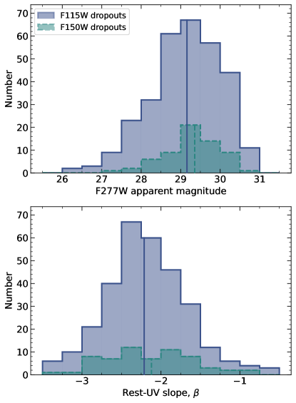
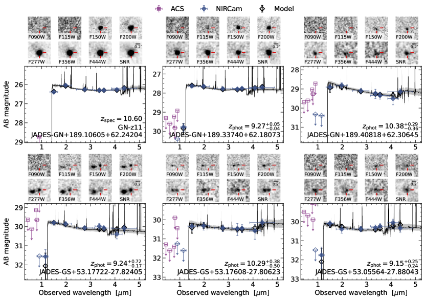
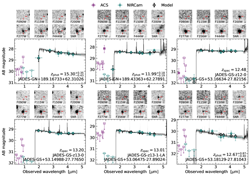
Our 309 F115W dropout candidates span nearly a factor of 100 in flux (almost five magnitudes) with F277W apparent magnitudes ranging from (median ; top panel of Figure 2). As is typical for galaxies (e.g. Wilkins et al., 2011; Finkelstein et al., 2012; Bouwens et al., 2014; Cullen et al., 2023; Austin et al., 2024; Topping et al., 2024; Saxena et al., 2024), the rest-frame UV continuum slopes () of the sample, measured by fitting power laws of the form to the observed F200W, F277W, and F356W photometry, are generally blue (median ; bottom panel of Figure 2). To minimize the likelihood of artificially reddening our inferred UV slopes, we do not use F150W (the filter immediately adjacent to the F115W dropout filter) to calculate , as this filter may be partially impacted by a Ly break or damped Ly absorption. We show the distributions of F277W apparent magnitudes and rest-UV slopes of the sample in Figure 2 and examples of the images and SEDs of individual objects in Figure 3.
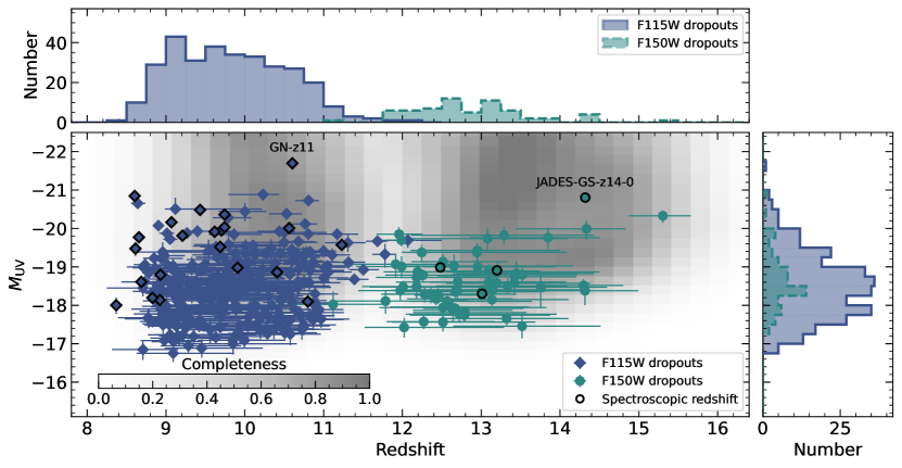
From the SED models, we infer redshifts from BEAGLE ranging from (median ) and absolute UV magnitudes of (median ). As shown in Figure 4, these inferred properties are consistent with expectations for the sample based on the selection function calculated as described in Section 5.1. We also highlight that most objects in the sample have large probabilities of being at . All candidates are guaranteed to have integrated probabilities of by the selection (Section 3) but most easily exceed this requirement and 83 percent of the candidates without a known spectroscopic redshift have .
4.2 F150W dropouts
Our 63 F150W dropout candidates also represent a large range of fluxes (a factor of , or magnitudes), and generally have blue rest-UV slopes (measured by fitting a power law to the observed F277W, F356W, and F444W photometry). We show examples of individual objects in Figure 5. As seen in Figure 2, the F150W dropout sample is observed with a median rest-UV slope of and F277W magnitudes of (median ). Correspondingly, we measure absolute UV magnitudes of (median ) at redshifts of (median ); see Figure 4. We again note that many of the F150W dropouts have high-redshift probabilities significantly larger than is required by the selection. Of the objects that are not spectroscopically confirmed, 55 percent have integrated high-redshift probabilities of .
4.3 Comparison with Hainline et al. (2024a)
In this work, we have adopted color selections to identify high-redshift galaxy candidates with which to measure the UV luminosity function. We now briefly compare these color-selected samples to the sample of candidates that were identified in JADES imaging by Hainline et al. (2024a) using photometric redshifts from EAZY. We note that Hainline et al. (2024a) searched for candidates at while our color selections are sensitive to candidates starting at a slightly higher redshift. We also note that the data presented in this work includes JADES imaging observed after the publication of Hainline et al. (2024a). Thus, to ensure consistency for this comparison, we only consider the subsets of the two samples that lie in the shared area at (spectroscopic redshifts if available, otherwise best-fit photometric redshifts from EAZY for the Hainline et al. 2024a sample and median photometric redshifts from BEAGLE for the objects in this work). After applying these requirements, we find that the color selections identify a moderately smaller number of galaxy candidates. Out of the parent sample of 372 color-selected candidates we have identified in this work, we find that 271 satisfy these criteria. In comparison, 327 of the full Primary Sample of 717 objects identified by Hainline et al. (2024a) satisfy the criteria. Of these candidates, 134 are shared between both selection methods.
We attribute this difference in part to the relatively low efficiency of color selections in specific ranges of redshift caused by the progressive redshifting of the Ly break through the dropout filters (see Hainline et al. 2024a for a quantitative discussion of this effect). At the redshifts where color selections are inefficient, the Ly break falls within a filter such that objects do not appear as complete dropouts in that filter. However, if that filter is used to calculate a rest-frame UV color while assuming the object is dropping out in the immediately adjacent, shorter wavelength filter, it appears to be red. Thus, such objects are not identified by either of the adjacent color selections but can be selected by their photometric redshifts. Additionally, we have required the photometry in at least three filters (four for the F115W dropouts) to be measured at , a slightly stronger S/N requirement than the one adopted by Hainline et al. (2024a).
For the objects that are identified by the color selection and are not included in the photometric redshift-selected sample, almost all have double-peaked redshift probability distributions, with peaks at both at and . Additionally, we find that approximately half of these sources also have best-fit EAZY redshifts at , but were removed from the Hainline et al. (2024a) sample by another selection criterion.
4.4 Comparison with Robertson et al. (2024)
The JADES imaging we use in this work encompasses the area of the JOF (Eisenstein et al., 2023b), in which Robertson et al. (2024) conducted a search for high-redshift galaxy candidates using a photometric redshift selection. We identify approximately the same number of objects in the JOF area using our F150W dropout color selection, but due to the differences in selection techniques, the objects included in the samples differ.
Of the eleven objects in the Robertson et al. (2024) Primary and Auxiliary samples at , our color selection shares six. The remaining five are all legitimate dropout candidates but three are removed by the bright neighbor flag that we apply in this work. The last two fall in between our F115W and F150W dropout selections with dropout colors that are slightly too blue to be identified by our color selection; this is the same effect as is seen when comparing our color selected sample to the photometric redshift selected sample of Hainline et al. (2024a). We also identify six F150W dropouts that are not included in the sample of Robertson et al. (2024) (including the Contributing and Auxiliary Samples), which were removed from the JOF luminosity function sample due to having a best fit photometric redshift from EAZY (Brammer et al., 2008) of in their catalog or an insufficiently large difference in the goodness-of-fit between the and photometric redshift solutions, but all of which also have secondary redshift solutions from EAZY at .
5 The rest-frame UV luminosity function
With our high-redshift candidate samples in hand, we now measure the UV luminosity function at and based on the F115W and F150W dropout samples and derive an upper limit at corresponding to our lack of F200W dropouts. We also estimate the binned luminosity function from a subset of the F150W dropout sample. In this section, we describe our methods for quantifying the completeness of our selection, then calculate binned and parametric forms of the UV luminosity function observed in the JADES fields.
5.1 Completeness
In order to accurately measure the UV luminosity function, we must account for the incompleteness of our selection. To this end, we perform source injection and recovery simulations designed to reproduce the real process of high-redshift galaxy selection as closely as possible. That is, we inject mock sources with a range of SEDs and morphological properties into the real JADES mosaics, then perform source detection, photometric measurements, and sample selection using the same methods as we use for our real data.
When creating artificial sources for injection, we sample properties from distributions designed to represent our current understanding of high redshift galaxy properties and to comfortably encompass the expected parameter space of our selections. Absolute UV magnitudes () are sampled from a uniform distribution in the range and redshifts () are sampled from uniform distributions with lower and upper bounds appropriate for each dropout selection (, , and for the F115W, F150W, and F200W dropout selections, respectively). Then, given for each mock source, we construct power law SEDs of the form , where is the rest-frame UV continuum slope. At the redshifts we consider in this work (), we expect to be primarily probing the rest-UV with our observational filter set and do not expect significant deviations from a power law shape of the SED due to strong emission lines, as the strongest rest-frame optical nebular emission lines (H, H, and the [O iii]4959,5007 doublet) have redshifted out of the filters we consider in this work and the strongest rest-frame UV emission line, Ly, is observed to be relatively uncommon at these redshifts (e.g. Nakane et al., 2024; Jones et al., 2024a, b; Tang et al., 2024; Napolitano et al., 2024b). The rest-UV slope is then determined from the mock source’s using the relation found by Topping et al. (2024), which follows a similar trend as other JWST measurements of the relation (e.g. Cullen et al., 2023, 2024; Austin et al., 2024). We note that Topping et al. (2024) derives relations for F115W dropouts and F150W dropouts but does not fit a relation for F200W dropouts, so we adopt the F150W dropout relation for both our F150W and F200W dropout selections. The SED is then normalized to at Å and redshifted to the observed frame at redshift . Finally, the IGM attenuation model of Inoue et al. (2014) is applied and mock source fluxes in the same ACS and NIRCam filters as are in the real photometric catalog are calculated by integrating the SED over the appropriate filter bandpasses. We note that, though the Inoue et al. (2014) IGM attenuation model does not explicitly consider the impact of damped Ly absorption, we do not expect strong damped Ly absorption to significantly impact our inferred UV luminosity functions. For the objects in our samples with spectroscopic redshift measurements, we observe only a mild systematic offset between the photometric and spectroscopic redshifts (median , consistent with expectations from larger samples Heintz et al., 2024), which is expected to have a negligible impact on the inferred UV luminosity ( mag).
To simulate source shapes, we assume Sérsic (1963) profiles with Sérsic indices () drawn from a one-sided truncated normal distribution with mean of , , and a minimum of . We draw the axis ratio (the ratio of the minor axis to the major axis, ) from a truncated normal distribution with mean of , standard deviation of , minimum of , and maximum of . Finally, we draw position angles from a uniform distribution ranging from to . To set galaxy sizes, we use the rest-UV size-luminosity relation found by Shibuya et al. (2015) (which has the same slope and very similar normalizations as size-luminosity relationships derived using JWST; Yang et al., 2022; Ono et al., 2023, 2024; Morishita et al., 2024) to calculate the half-light radius () for a mock galaxy with given UV luminosity and redshift. Simulated images of these mock sources are generated using GalSim (Rowe et al., 2015) and placed into the real JADES mosaics. We then repeat our process of detection, photometric measurements, and selection (Sections 2.2 and 3) on the mosaics containing the mock sources. We also measure the absolute UV magnitudes of the recovered mock sources following the same methods we have used for the real objects (Section 4).
We calculate the combined completeness of our detection and selection methods, , as a function of absolute UV magnitude and redshift marginalized over all other source properties. However, we highlight that the UV luminosity function is a function of true , , while we can only observe a recovered absolute UV magnitude, , and is not guaranteed to be the same as . To account for this difference, we quantify our selection completeness as a function of both true and recovered absolute UV magnitude as well as true redshift (similar to methods adopted by, e.g. Bouwens et al., 2021; Leethochawalit et al., 2023). Thus, completeness is defined as
| (1) |
where is the number of objects that have been injected in a given bin of true absolute UV magnitude and redshift, (), and is the number of sources that were originally injected into that same bin and were recovered with an absolute UV magnitude of .
We find that our detection and selection methods recover our injected sources with reasonably high completeness for the luminosities we use to calculate the luminosity function. In the brightest bins and central redshifts of our selection functions where we expect to be most complete, we find a maximum completeness of percent due to objects overlapping with other sources and photometric scatter. At its central redshifts () and in the deepest subregion of the imaging ( s), our F115W dropout selection is percent complete in the faintest bin we use to calculate the UV luminosity function (centered at ). For the F150W dropouts, which is maximally complete at , we find completeness of percent in the faintest bin (centered at ) and deepest subregion.
Using this definition of the completeness, the effective volume of the survey is also a function of both true and recovered :
| (2) |
where is the differential comoving volume element in the survey area at redshift . Then, given a UV luminosity function, , the number of objects expected as a function of can be calculated.
Starting from a given bin of true , , the number of objects expected to be measured with is . Then, the total number of objects in the bin is simply the sum of the contributions from all bins:
| (3) |
Alternatively, this quantity can be thought of as the element of the dot product of the binned UV luminosity function, , and the matrix of effective volumes, , which produces a vector of expected counts as a function of :
| (4) |
where denotes the element-wise (Hadamard) product of matrices.
Thus, we can now relate the luminosity function as a function of true (an unobservable quantity) to the number of objects expected in the sample as a function of recovered (the observable quantity), and fit the UV luminosity function.
5.2 The binned UV luminosity function
| [mag] | [ mag-1 Mpc-3] |
|---|---|
| F115W dropouts () | |
| F150W dropouts () | |
| F150W dropouts, () | |
| F200W dropouts, | |
We calculate the luminosity function for each of the three dropout samples we consider in this work rather than in bins of redshift to avoid mixing objects between samples. Photometric redshifts can be highly uncertain, so calculating the UV luminosity function in bins of redshift requires joint fitting of the luminosity function at all redshifts under consideration to account for objects scattering between redshift bins.555For example, if we were to calculate luminosity functions from and , an object with a photometric redshift of may reasonably be expected to contribute to either one. However, observed candidates do not scatter between the dropout samples, so we can separately calculate the binned luminosity function for each dropout sample (which correspond to redshift ranges of , , and for the F115W, F150W, and F200W dropouts, respectively). To investigate the evolution of the luminosity function at , we also use a subset of the F150W dropout sample and the corresponding estimate of the completeness of the F150W dropout selection at to estimate a luminosity function.
For the binned F115W dropout, F150W dropout, and F150W dropout UV luminosity functions, we use a Markov chain Monte Carlo (MCMC) algorithm to sample the posterior probability distributions for the number densities in each bin of . The set of binned number densities, , comprises the parameters for which we are fitting. To calculate the upper limit on the F200W dropout UV luminosity function, we adopt the same bins as for the F150W dropout luminosity function, then simply calculate , where is the single-sided upper limit for assuming Poisson statistics (Gehrels, 1986).
We adopt a Poisson likelihood function for the number of objects in each bin of , as is appropriate for the relatively small counts in some of the bins at higher redshifts. Thus, the log-likelihood function for the bin is
| (5) |
where is the natural logarithm of and is the factorial of . is the number of objects that are observed to have absolute UV magnitudes that fall within the bin and is the expected number of galaxies in the same bin. The total log-likelihood for the luminosity function is then the joint log-likelihood of all of the bins (the sum of Equation (5) over all bins):
| (6) |
We note that, as described in Section 5.1, the luminosity function is a function of true , but we will evaluate this likelihood in bins of recovered with calculated from using Equation (3).
| Parameterization | |||||
|---|---|---|---|---|---|
| [ mag-1 Mpc-3] | [mag] | [erg s-1 Hz-1 Mpc-3] | |||
| F115W dropouts | |||||
| Schechter | — | ||||
| DPL | |||||
| F150W dropouts | |||||
| Schechter | — | ||||
| DPL | |||||
We also note that the observed absolute UV magnitude of a real object may be uncertain due to both photometric scatter in the observed SED and uncertainties in the photometric redshift. Thus, we do not assign each observed candidate one value of observed . Rather, we account for uncertainties in observed by drawing one sample from every observed object’s posterior, calculated as described in Section 4, at each step in the MCMC. This produces a set of observed absolute UV magnitudes (one for each object in the sample), which we use to calculate for the step. For the subset of the F150W dropouts, we perform a similar sampling of both redshift and from each of the F150W dropouts, but only use objects with a sampled redshift of at each step.
We sample the binned luminosity functions using a Metropolis-Hastings algorithm (Metropolis et al., 1953; Hastings, 1970). We adopt Gaussian proposal distributions with standard deviations tuned to obtain acceptance rates of , and run the MCMC for steps using 20 walkers. To initialize the samplers, we calculate an initial estimate for the binned number densities by calculating (where is counted using the median for each object) in each bin, then make small perturbations around this initial guess.
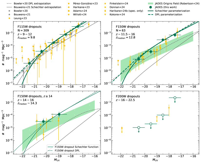
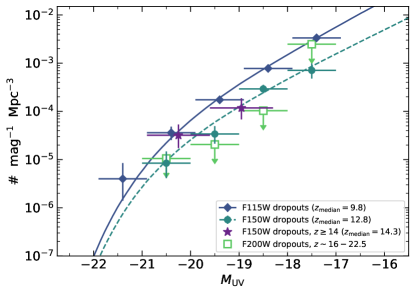
To estimate the final posterior distributions, we concatenate the chains from all 20 walkers, leading to a total of equally weighted samples. We take the median of the marginalized posterior distribution in each bin as the number density in that bin with uncertainties corresponding to the and percentiles. We show the resulting binned UV luminosity functions in Figure 6 and report the values in Table 5 for the F115W, F150W, and F200W dropout samples. For comparison, we also show in Figure 6 the luminosity functions implied by the fits for the redshift evolution of the Schechter (Bouwens et al., 2021) and double power law (DPL; Bowler et al., 2020) parameters (based on HST and ground-based data) along with measurements of the UV luminosity function from the literature. In Figure 7, we show a comparison of all three dropout samples along with the subset of the F150W dropouts. For each dropout selection, we show measurements closest to the median redshift of the selection (typically or and or for the F115W and F150W dropout samples, respectively).
Our measurements are generally consistent with most JWST constraints on the UV luminosity function (e.g. Harikane et al., 2023; Leung et al., 2023; Pérez-González et al., 2023; Finkelstein et al., 2024; Willott et al., 2024; Adams et al., 2024; Donnan et al., 2024), especially for the F115W dropouts, with smaller uncertainties. While there are fewer measurements at the redshifts of the F150W dropouts and at , we also find consistency with the binned data points of Pérez-González et al. (2023) at all luminosities where the datasets overlap, and broad agreement with other studies at luminosities brighter than . At fainter luminosities, the F150W dropout luminosity function is slightly higher than some studies. Notably, our F150W dropout luminosity function is higher than was measured in the JOF (Robertson et al., 2024) by a factor of . We attribute this difference to several factors, discussed in more detail in Section 5.5. Finally, our upper limit on the F200W dropout luminosity function is approximately consistent with the upper limit measured by Harikane et al. (2024b) at and the upper limit measured by Kokorev et al. (2024) at . However, we note that the measurement by Kokorev et al. (2024) at based on five galaxy candidates implies the presence of galaxies in the JADES fields at (where we found none). This could be due to effects such as cosmic variance or simply Poisson noise, but we note that our upper limit combined with the measurement by Kokorev et al. (2024) requires an extremely rapid increase in the abundance of galaxies between and . If confirmed to be a physical effect, this is a significant change from the shape of the luminosity function we find at and implies a rapid evolution in star formation processes between and , and we emphasize the need for spectroscopic observations for confirmation.
Ultimately, we measure the luminosity function over a large range of luminosity (five magnitudes or a factor of 100 in luminosity for the F115W dropouts, and four magnitudes or a factor of in luminosity for the F150W dropouts), enabling us to self-consistently examine the luminosity function and evolution thereof for both bright and faint galaxies. Overall, we measure number densities at that are slightly higher than pre-JWST expectations over the full range of luminosities we have probed in this work, a difference that grows larger at increasingly high redshifts. We observe essentially no evolution between the full F150W dropout sample and the subset.
5.3 The parametric UV luminosity function
We also fit parametric forms of the UV luminosity function. We assume a Schechter (1976) function666
as our fiducial parameterization, which has long been standard for the high-redshift UV luminosity function. However, at high redshifts (), there is evidence that bright () galaxies are in excess of the exponential decline of the Schechter function and the high-redshift UV luminosity function may be better represented by a double power law (DPL) parameterization777 (e.g. Bowler et al., 2020; Donnan et al., 2024) with characteristic luminosities around . While our data do not reach extremely bright luminosities () due to the limited area of the survey, we observe objects at , enabling us to also fit a DPL to facilitate comparisons with other studies.
To fit the parametric luminosity function, we again use an MCMC algorithm to sample the probability distributions of the parameters for the functional form under consideration. For the Schechter function, we are fitting for the overall normalization (), the characteristic UV luminosity (), and the faint end slope (). For the DPL, we are fitting for the same parameters plus the bright end slope (). We place uniform priors on all parameters with the following ranges: , , , and for the DPL, . We then use the same Metropolis-Hastings algorithm as described in Section 5.2 to sample the function parameters, again with steps and 20 walkers with proposal distributions tuned to obtain acceptance rates of . To use Equation (6) as the likelihood function, we convert the continuous function to a binned luminosity function with bins of width , from which we can calculate expected counts.
For the F115W dropouts, we fit for all of the free parameters of the luminosity function. For the F150W dropouts, we fix the characteristic luminosity () to the value that we find for the F115W dropouts due to the presence of JADES-GS-z14-0 in our sample and the more restricted luminosity range of the F150W dropouts. For the subset of the F150W dropout luminosity function and the F200W dropouts, we fix all parameters except the normalization () to the values of the F150W dropout luminosity function. We report the final constraints on the Schechter and DPL parameters in Table 6 and show the median of the fits marginalized over all of the function parameters in Figure 6.
For the F115W dropout Schechter function, we find a characteristic UV magnitude of (similar to or slightly fainter than other measurements), a normalization of mag-1 Mpc-3 (higher than expected from most pre-JWST measurements and consistent with JWST constraints), and a steep faint end slope of (generally consistent with pre-JWST extrapolations but steeper than most JWST measurements). Compared to the Schechter function, when assuming a DPL, we measure a slightly brighter characteristic luminosity (), correspondingly lower normalization ( mag-1 Mpc-3), and moderately steeper faint end slope (). The normalization of the F150W dropout luminosity function declines by a factor of from the F115W dropout luminosity function to mag-1 Mpc-3 and mag-1 Mpc-3 for the Schechter function and DPL, respectively. We continue to find steep faint end slopes of and at . In general, we find similarly high normalizations of the UV luminosity function as other JWST constraints, but slightly steeper faint end slope (see Section 6.2), and combined, this leads to a relatively slow decline in the cosmic UV luminosity density over time as discussed below.
5.4 The cosmic UV luminosity density
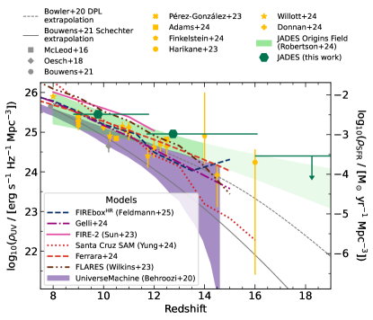
We calculate the cosmic UV luminosity density, , as the luminosity-weighted integral of the Schechter parameterizations of the F115W and F150W dropout luminosity functions. We show the resulting values of in Figure 8. For the F200W dropout upper limit, we take the luminosity-weighted integral of the binned values of the upper limit on the luminosity function between and . The DPL parameterization systematically implies moderately higher values of than the Schechter functions, but both parameterizations are consistent within errors. We also convert to the cosmic star formation rate density () using the commonly adopted conversion factor (M⊙ yr-1) / (erg s-1 Hz-1) (Madau & Dickinson, 2014), which assumes a Salpeter (1955) stellar initial mass function. We report the values of obtained when integrating to the frequently assumed faint limit of and emphasize that the JADES luminosity function measurement extends down to ; thus, calculating does not require any extrapolation.
From the F115W dropouts (), we find a cosmic UV luminosity density of erg s-1 Hz-1 Mpc-3, which declines by a factor of between and (probed by the F150W dropouts) to erg s-1 Hz-1 Mpc-3, then further declines by another factor of to be erg s-1 Hz-1 Mpc-3 for the F200W dropout upper limit. As expected from the high normalization and steep faint end slopes, these UV luminosity densities are slightly higher than measurements based on HST and ground-based data at , with increasing tension at .
5.5 Comparison with the JOF UV luminosity function
We now briefly compare our luminosity function to that measured by Robertson et al. (2024) in the JOF. As introduced in Section 5.2, we find higher number densities at in this work compared to Robertson et al. (2024), which may be due to several factors.
First, while both the JOF sample and our sample include the very bright, galaxy JADES-GS-z14-0, the JADES area we consider in this work is nearly 20 times larger than the JOF area (i.e. the surface density implied by JADES is lower than that implied by JOF). This then raises the median of the bright end of the JOF luminosity function above what we measure over the full JADES area. Then, due to the parameterization of the JOF luminosity function as an evolving Schechter function, which explicitly ties the behavior of the bright and faint regimes of the luminosity function together, this influences the luminosity function measured in the JOF area to trend towards a shallower faint end slope and therefore lower number densities at in the absence of large numbers of faint objects. In other words, when assuming a parametric form of the luminosity function, the presence of an unusually bright object (JADES-GS-z14-0) driving the bright end to higher number densities induces a difference between the JOF luminosity function and this work at the faint end. This difference may be further influenced by the fitting method that Robertson et al. (2024) used that quantitatively accounts for how low luminosity objects with uncertain colors or photometric redshifts may scatter into higher redshift samples, which our analysis does not explicitly model.
Second, the method used by Robertson et al. (2024) to calculate the luminosity function uses the full photometric redshift likelihoods of the observed objects. In comparison, we use the entire photometric redshift probability distributions for selection and remove objects that we find have an integrated probability percent of being at low redshift (based on BEAGLE models; Section 3). We then consider only high-redshift solutions when calculating our luminosity function (Section 5.2), which assumes that our selection identifies high-redshift candidates with a low contamination rate (noting that we find a relatively small percent spectroscopic contamination rate for the objects in our sample that have spectroscopic redshifts). Incorporating the photometric redshift distributions while fitting the luminosity function accounts for redshift uncertainties probabilistically, which may lead to differences, particularly at the faint end where photometric measurements and therefore inferred quantities are more uncertain. For instance, there are five objects in our sample in the JOF area with that do not satisfy the selection criteria used by Robertson et al. (2024) and are not used in the calculation of the JOF luminosity function. Of those objects, Robertson et al. (2024) found that two are best fit at low redshifts of (based on EAZY) and the other three are best fit at high redshift but have low redshift peaks in their redshift probability distributions such that the difference in the goodness-of-fit between the best-fit low- and high-redshift solutions is . In this work, though they are less well characterized than brighter systems, these objects satisfy our photometric redshift requirement (having an integrated low-redshift probability of less than 50 percent from BEAGLE models), and ultimately, illustrate the need for spectroscopy to confirm the redshifts of faint objects.
Third, we calculate both our detection and selection completeness correction with end-to-end source injection and recovery simulations. In comparison, Robertson et al. (2024) used source injection simulations to measure detection completeness and then used Monte Carlo simulations of SED models to compute their selection completeness. Both methods may face different systematic uncertainties.
6 Discussion
In this work, we have used deep JWST imaging from JADES to identify galaxies to faint UV magnitudes of and constrain the UV luminosity function down to luminosities up to 40 times fainter than the characteristic luminosity at these redshifts. Using this powerful dataset, we can now begin to examine implications for early galaxy evolution and the reionization process.
6.1 Comparison with theoretical predictions
Within just a few months of starting scientific operations, JWST enabled the discovery of several galaxies at in relatively small survey areas (e.g. Naidu et al., 2022; Castellano et al., 2022; Donnan et al., 2023; Finkelstein et al., 2022b). Though comprising only a few objects with large uncertainties from both Poisson errors and cosmic variance, this tentatively suggested the existence of a surprisingly large number of bright galaxies. Subsequently, statistical measurements of the UV luminosity function have confirmed the presence of a large bright galaxy population at (e.g. Adams et al., 2023; Harikane et al., 2023, 2024a, 2024b; Finkelstein et al., 2023; McLeod et al., 2024; Donnan et al., 2024). However, while there is now a general consensus that JWST has observed an excess of bright () galaxies at relative to expectations from pre-JWST theoretical models, it is less clear if that excess is also observed in the galaxy population.
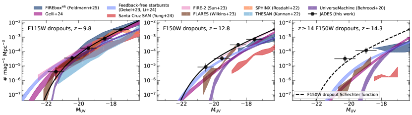
In Figure 9, we compare our measurement of the UV luminosity function to a variety of theoretical models. We emphasize that our measurement of the luminosity function simultaneously reaches both relatively bright luminosities () and the faintest luminosities accessible to date in blank fields (), allowing us to probe the full shape of the high-redshift luminosity function. We refer back to Figure 8 for comparisons to model predictions of the cosmic UV luminosity density.
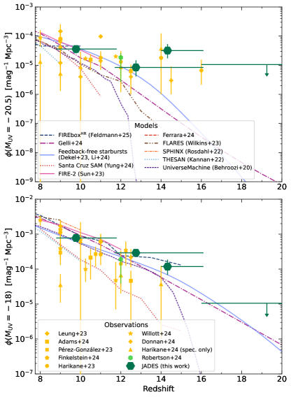
As has been found by other JWST studies of the luminosity function, we find a significant excess of galaxies over expectations from many models at . Notably, this excess is observed not only for models calibrated to data before JWST (FLARES, SPHINX, THESAN, and UniverseMachine, shown with hatches in Figure 9), but is also present for some of those that successfully reproduce JWST observations at (top panel of Figure 10). Moreover, we highlight that we also observe high number densities at faint UV luminosities (), especially at higher redshifts (bottom panel of Figure 10), though the excess is smaller at the faint end than the bright end. That is, the galaxy population at any luminosity within the regime we have probed within this work () is at least slightly larger than most theoretical predictions and the abundance of galaxies is just one realization of a systematic trend that extends to fainter luminosities. The exact degree of this excess, as well as its luminosity and redshift dependence, can help constrain the physical mechanisms that regulate star formation in the early Universe.
Many of the processes proposed to explain the abundance of galaxies at , such as bursty star formation (e.g. Mason et al., 2023; Mirocha & Furlanetto, 2023; Shen et al., 2023; Sun et al., 2023; Kravtsov & Belokurov, 2024; Gelli et al., 2024) and/or a higher star formation efficiency than expected at high redshift (e.g. Dekel et al., 2023; Li et al., 2024; Harikane et al., 2023; Ceverino et al., 2024; Feldmann et al., 2025), either of which may lead to an increase in the average light-to-stellar mass ratios with redshift (e.g. Donnan et al., 2024), predict different behavior for the faint end of the luminosity function. For example, as seen in Figure 9, the faint end slope of the UV luminosity function predicted by the feedback-free starburst model (Dekel et al., 2023; Li et al., 2024) is shallower than many other models that can match the UV luminosity function at . Thus, though the predicted bright end of the higher redshift, luminosity function approximately matches our measurement, it becomes inconsistent at . In contrast, the steep slope of the predicted luminosity function from FLARES (Wilkins et al., 2023) is in strong tension with our observations at but agreement at . Moreover, the FIREbox model (Feldmann et al., 2025) explicitly predicts an increasingly steep faint end slope at higher redshifts. In the future, full constraints on the abundance of both bright and faint galaxies, and ultimately the shape of the luminosity function and evolution thereof, will be crucial for understanding star formation processes in early galaxies.
6.2 Implications for reionization
In addition to providing insights into early galaxy evolution, the UV luminosity function has important implications for cosmic reionization, as it contributes to setting the total number of ionizing photons produced by galaxies that are available to reionize the Universe. Notably, in this work, we have measured not only a high normalization of the UV luminosity function consistent with other measurements from JWST, but also a steeper faint end slope than has been found by many other studies. Together, this implies the existence of a large population of UV-faint galaxies and a commensurately large non-ionizing UV luminosity density at very early times. If this large population of far-UV-continuum–faint galaxies also produces ionizing photons that can escape into the IGM at any significant rate, such systems could be appreciably reionizing the Universe as early as .
To investigate the implications of the faint galaxy population for reionization, we calculate the reionization history as the time evolution of the volume-averaged fraction of neutral hydrogen in the IGM, . In practice, we quantify the neutral fraction in terms of the volume-averaged ionized hydrogen fraction, , as . At its simplest, is governed by the following differential equation (Madau et al., 1999), where dots denote time derivatives:
| (7) |
which describes the competing effects of photoionizations of intergalactic neutral hydrogen and recombinations of free electrons with protons to (re)form neutral hydrogen. The average comoving number density of hydrogen, , depends on the primordial mass fraction of hydrogen (), the fractional baryon density parameter (), the critical density (), and the mass of hydrogen (). The timescale of recombinations in the IGM at a given time, , can be calculated as
| (8) |
is a “clumping factor” that accounts for inhomogeneities in the IGM and we choose to fix (consistent with theoretical expectations from simulations; e.g. Shull et al., 2012; Finlator et al., 2012; Kaurov & Gnedin, 2015; Gorce et al., 2018). is the case B recombination coefficient for hydrogen and we assume a temperature of K, giving cm3 s-1 (Draine, 2011). is the comoving free electron number density assuming single ionized helium and a primordial helium mass fraction of , and is the redshift at time .
Finally, is the hydrogen ionizing photon production rate per unit comoving volume at a given time (i.e. the ionizing photon emissivity) that depends on the non-ionizing UV luminosity of the galaxy population, the ionizing photon production rate per unit non-ionizing UV luminosity (i.e. the ionizing photon production efficiency; ), and the fraction of all hydrogen ionizing photons produced by the ionizing sources, here assumed to be galaxies, that escape into the IGM (i.e. the escape fraction, ). When both and are independent of UV luminosity, the non-ionizing UV luminosity term is the cosmic UV luminosity density, , giving
| (9) |
In this work, we also allow to depend on UV luminosity (and can also allow to be luminosity dependent), so Equation (9) becomes
| (10) |
where is the UV luminosity function at time . To isolate the effects of the UV luminosity function on the reionization timeline, we choose to assume a constant escape fraction with as our fiducial value (approximately similar to Lyman continuum escape fractions observed in samples with similar UV luminosities and UV continuum slopes as we study in this work; e.g. Izotov et al., 2021; Chisholm et al., 2022; Mascia et al., 2024; Rinaldi et al., 2024) and adopt the relation at found by Endsley et al. (2024). This relation has the primary features of a decrease in the average and an increase in the scatter of with decreasing UV luminosity, though we note that even at the faintest UV luminosities studied, the median is moderately higher than the often used “canonical” value of Hz erg-1 informed by Bruzual & Charlot (2003) stellar population synthesis models matched to observed UV colors (Robertson et al. 2013, though also see Bouwens et al. 2016; De Barros et al. 2019; Lam et al. 2019; Rinaldi et al. 2024 for discussions of higher values of for high-redshift star forming galaxies).
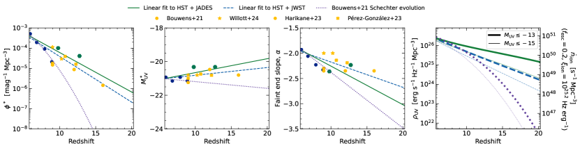
To obtain , we assume a Schechter function and fit the redshift evolution of the Schechter parameters, assuming that , , and all evolve linearly with redshift. As we wish to evaluate the impact of the steep faint end slope we have found in this work, we perform two fits for the redshift evolution of the Schechter parameters, which will determine : one fit to a compilation of measurements of the Schechter parameters from the literature at from both HST and JWST and a second fit using only the JADES data combined with HST. We also compare to the Schechter parameter evolution found by Bouwens et al. (2021), who fit as a quadratic function with redshift and and as linear functions.
We show the resulting evolutionary fits for the Schechter parameters along with the implied cosmic UV luminosity density integrated to in Figure 11. For illustrative purposes, we also show the ionizing photon emissivity corresponding to the cosmic UV luminosity density for fixed and Hz erg-1 as the right axis of the rightmost panel. Though we do not assume these values when calculating the reionization history, it has been shown that these assumptions are sufficient to reionize the Universe when integrating UV luminosity functions from HST down to (Robertson et al., 2013, 2015). When fitting the evolution of the Schechter function parameters with a large compilation of JWST data combined with HST, we find a slower redshift evolution of the faint end slope than when we use only JADES data combined with HST measurements; this is due to the slightly shallower faint end slopes found by many JWST studies compared to the steep faint end slopes we find from JADES at . At , the HST and JADES fit predicts a faint end slope of while the fit including HST and other JWST data gives . Combined with the high overall normalization of the luminosity function at , this implies that the cosmic UV luminosity density can remain large at early times, potentially allowing the escape fractions and/or ionizing photon production efficiencies necessary to drive reionization to be lower than were thought necessary prior to JWST.
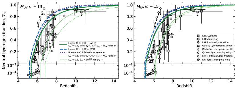
With all components of Equation (7) thus calculated, we can integrate forward in time to obtain the reionization history. We start the integration at and show the resulting reionization histories in Figure 12 alongside observational constraints on the neutral fraction from galaxies and quasars. We note that the reionization history does not significantly depend on the starting redshift due to the normalization of the luminosity function decreasing to be vanishingly small at . We show the results of integrating Equation (10) all the reionization histories resulting from all of the luminosity function evolution fits assuming an escape fraction of . We also show the reionization history assuming and the HST and JADES luminosity function evolution fit to demonstrate the impact of changing the escape fraction.
We first highlight that, despite the steep faint end slope of the luminosity function and the implied large population of faint galaxies, this simple estimate of the reionization timeline is naturally in broad agreement with observational constraints on the end of reionization (see Fan et al., 2023, and references therein). When considering galaxies down to luminosities of and an escape fraction , all three luminosity function fits complete reionization at . When only considering contributions from galaxies, reionization ends at .
We acknowledge that the ionizing photon emissivity depends on and as well as . We have adopted specific parameterizations for both of these quantities and choosing other physically plausible values can impact the reionization history. For example, at fixed escape fraction, adopting the Simmonds et al. (2024) relation for ends reionization slightly later than our fiducial model based on Endsley et al. (2024). Increasing the escape fraction to or fixing to a constant value of Hz erg-1 (consistent with the findings of Atek et al. 2024 for a sample of faint galaxies) increases to the extent of driving reionization faster than is allowed by strong constraints on the timing of reionization placed by the cosmic microwave background (see discussion by Muñoz et al., 2024). However, we emphasize that our fiducial assumptions, which were chosen to be approximately consistent with observations of early galaxies, can comfortably give rise to a reionization history that ends in time to be compatible with observations (or at least not well before). This suggests that current observations of the ionizing properties of high-redshift galaxies are broadly consistent with constraints on the reionization timeline. Thus, we conclude that galaxies can drive the reionization process without overproducing ionizing photons, even if there is a large population of faint galaxies.
While all of the luminosity function fits predict similar evolutions of the neutral fraction near the end of reionization (), the early stages of reionization proceed differently. If , both the HST-based luminosity function evolution (Bouwens et al., 2021) and our evolutionary fit to HST and many JWST luminosity functions lead to a nearly entirely neutral IGM at ( for both and ). However, when considering HST combined only with JADES, the combination of a steep faint end slope and high normalization leads to reionization starting earlier, and correspondingly, progressing slightly more slowly in order to end at . Under these circumstances, though the IGM is very neutral at , it is not quite fully neutral ( and at when integrating to and , respectively) – a scenario that would also be consistent with the remarkable discoveries of two galaxies emitting Ly at (Bunker et al., 2023; Witstok et al., 2024) and the implied neutral fraction of (e.g. Bruton et al., 2023; Nakane et al., 2024; Tang et al., 2024; Umeda et al., 2024).
Above, we have explored the role of the UV luminosity function in determining the reionization timeline. Given empirically motivated assumptions for the production and escape of ionizing photons from galaxies and the evolution of the UV luminosity function implied by our findings in this work, we have found that it is feasible for the IGM to be appreciably ionized only Myr after the Big Bang while still being compatible with observations at the conclusion of reionization. However, fully determining the reionization timeline will require even better constraints on the abundances and properties of early galaxies. In the future, combining deep imaging with JWST in lensing fields, which can reach extremely faint luminosities to constrain the faint end turnover and increase the dynamic range of luminosities available to measure the faint end slope, with imaging in blank fields over larger areas, which provides insights into the brighter galaxies. Together, these observations will provide robust constraints on the shape of the entire luminosity function and enable us to directly characterize the ionizing properties of early galaxies.
7 Summary
In this work, we have used deep NIRCam imaging from the JADES program to measure the high-redshift UV luminosity function down to faint luminosities of . We search for high-redshift galaxy candidates at (and identify candidates at ), measure their properties, infer both binned and parametric forms of the UV luminosity function, and discuss the implications of our results for early galaxy evolution and cosmic reionization. We summarize our key findings below.
-
(i)
We conduct a search for galaxy candidates using three dropout filters: F115W (probing ), F150W (), and F200W (). We color select 309 F115W dropouts, 63 F150W dropouts, and zero F200W dropouts for a total of 372 candidates over 163 arcmin2 of JADES NIRCam imaging. The objects we select span nearly five magnitudes and generally have the blue rest-UV continuum slopes of that are expected for high-redshift galaxies.
-
(ii)
We use four bins of redshift to calculate the UV luminosity function: three corresponding to the dropout filters used for selection and one isolating the subset of from the F150W dropouts. At (F115W dropouts), we measure the luminosity function at . At (all F150W dropouts) and (the subset of the F150W dropouts), we constrain the luminosity function at and , respectively. We also place an upper limit on the UV luminosity function at based on the absence of F200W dropouts. Using this large dynamic range of UV luminosities enabled by the deep JADES imaging over a moderately large area, we can simultaneously constrain the bright and faint end of the luminosity function. We find number densities in general agreement with other measurements of the high-redshift UV luminosity function from JWST but measure moderately steeper faint end slopes ( at ).
-
(iii)
Our measurement of the UV luminosity function is broadly consistent with models at , but lies above theoretical expectations for the UV luminosity function at at all luminosities. Thus, for a given parent population, the average UV luminosity is higher than expected, and the abundant bright galaxy population is a realization of a systematic trend that extends to fainter luminosities.
-
(iv)
The combination of a high normalization and steep faint end slope implies that there may be a large population of faint galaxies contributing ionizing photons towards ionizing the Universe. We therefore estimate the reionization history with our measurement of the UV luminosity function and physically motivated assumptions for ionizing photon production efficiencies and escape fractions. Given these simple assumptions, the reionization process can end at (consistent with observations at the end of reionization), even with a large faint galaxy population. However, the reionization process can start earlier, leading to volume-averaged neutral hydrogen fractions of even at , which may be consistent with observations of individual Ly emitters at these redshifts.
-
(v)
We highlight the importance of future deep observations to fully characterize the faint galaxy population and their contribution to reionization. Observations in lensing fields that are sensitive to significantly fainter luminosities than we have probed in this work, combined with additional deep imaging in blank fields covering larger areas, will be crucial to fully and robustly constrain the faint end slope and the turnover of the UV luminosity function.
Acknowledgments
The authors thank the SPHINX collaboration, the THESAN collaboration, Peter Behroozi, Robert Feldmann, Viola Gelli, Zhaozhou Li, Jason Sun, Steve Wilkins, and L.Y. Aaron Yung for providing their theoretical predictions for the luminosity function. LW also thanks Nick Schragal for helpful conversations throughout this work (and his dice collection for providing random number generator seeds).
LW, BR, MR, KNH, EE, DJE, JMH, ZJ, BDJ, and CNAW acknowledge support from the JWST/NIRCam contract to the University of Arizona, NAS5-02015. LW also acknowledges support from the National Science Foundation Graduate Research Fellowship under Grant No. DGE-2137419. BR acknowledges support from JWST Program 3215. WMB acknowledges support by a research grant (VIL54489) from VILLUM FONDEN. AJB and JC acknowledge funding from the “FirstGalaxies” Advanced Grant from the European Research Council (ERC) under the European Union’s Horizon 2020 research and innovation program (Grant agreement No. 789056). S. Carniani acknowledges support by European Union’s HE ERC Starting Grant No. 101040227 - WINGS. ECL acknowledges support of an STFC Webb Fellowship (ST/W001438/1). DJE is supported as a Simons Investigator. ZJ acknowledges funding from program JWST-GO-1963 that is provided by NASA through a grant from the Space Telescope Science Institute, which is operated by the Association of Universities for Research in Astronomy, Inc., under NASA contract NAS 5-03127. PGP-G acknowledges support from grant PID2022-139567NB-I00 funded by Spanish Ministerio de Ciencia, Innovación y Universidades MICIU/AEI/10.13039/501100011033, and the European Union FEDER program Una manera de hacer Europa. ST acknowledges support by the Royal Society Research Grant G125142. The research of CCW is supported by NOIRLab, which is managed by the Association of Universities for Research in Astronomy (AURA) under a cooperative agreement with the National Science Foundation. JW gratefully acknowledges support from the Cosmic Dawn Center through the DAWN Fellowship. The Cosmic Dawn Center (DAWN) is funded by the Danish National Research Foundation under grant No. 140.
This work is based on observations made with the NASA/ESA/CSA JWST. The data were obtained from the Mikulski Archive for Space Telescopes at the Space Telescope Science Institute, which is operated by the Association of Universities for Research in Astronomy, Inc., under NASA contract NAS 5-03127 for JWST. These observations are associated with programs 1180, 1181, 1210, 1286, 1287, 1895, 1963, and 3215. The authors acknowledge the FRESCO team led by PI Pascal Oesch for developing their observing program with a zero-exclusive-access period. We also acknowledge the Hubble Legacy Fields team for the reduction and release of the HST ACS imaging we use in this work.
The JADES Collaboration acknowledges support from JWST/NIRCam contract to the University of Arizona, NAS5-02015. This project made use of the lux supercomputer at UC Santa Cruz, funded by NSF MRI grant AST-1828315, as well as High Performance Computing (HPC) resources supported by the University of Arizona TRIF, UITS, and Research, Innovation, and Impact (RII) and maintained by the UArizona Research Technologies department.
We respectfully acknowledge the University of Arizona is on the land and territories of Indigenous peoples. Today, Arizona is home to 22 federally recognized tribes, with Tucson being home to the O’odham and the Yaqui. Committed to diversity and inclusion, the University strives to build sustainable relationships with sovereign Native Nations and Indigenous communities through education offerings, partnerships, and community service.
References
- Adams et al. (2023) Adams, N. J., Conselice, C. J., Ferreira, L., et al. 2023, MNRAS, 518, 4755, doi: 10.1093/mnras/stac3347
- Adams et al. (2024) Adams, N. J., Conselice, C. J., Austin, D., et al. 2024, ApJ, 965, 169, doi: 10.3847/1538-4357/ad2a7b
- Akhlaghi & Ichikawa (2015) Akhlaghi, M., & Ichikawa, T. 2015, ApJS, 220, 1, doi: 10.1088/0067-0049/220/1/1
- Arrabal Haro et al. (2023) Arrabal Haro, P., Dickinson, M., Finkelstein, S. L., et al. 2023, Nature, 622, 707, doi: 10.1038/s41586-023-06521-7
- Astropy Collaboration et al. (2013) Astropy Collaboration, Robitaille, T. P., Tollerud, E. J., et al. 2013, A&A, 558, A33, doi: 10.1051/0004-6361/201322068
- Astropy Collaboration et al. (2018) Astropy Collaboration, Price-Whelan, A. M., Sipőcz, B. M., et al. 2018, AJ, 156, 123, doi: 10.3847/1538-3881/aabc4f
- Astropy Collaboration et al. (2022) Astropy Collaboration, Price-Whelan, A. M., Lim, P. L., et al. 2022, ApJ, 935, 167, doi: 10.3847/1538-4357/ac7c74
- Atek et al. (2024) Atek, H., Labbé, I., Furtak, L. J., et al. 2024, Nature, 626, 975, doi: 10.1038/s41586-024-07043-6
- Austin et al. (2024) Austin, D., Conselice, C. J., Adams, N. J., et al. 2024, arXiv e-prints, arXiv:2404.10751, doi: 10.48550/arXiv.2404.10751
- Bañados et al. (2018) Bañados, E., Venemans, B. P., Mazzucchelli, C., et al. 2018, Nature, 553, 473, doi: 10.1038/nature25180
- Behroozi et al. (2020) Behroozi, P., Conroy, C., Wechsler, R. H., et al. 2020, MNRAS, 499, 5702, doi: 10.1093/mnras/staa3164
- Bertin & Arnouts (1996) Bertin, E., & Arnouts, S. 1996, A&AS, 117, 393, doi: 10.1051/aas:1996164
- Bolan et al. (2022) Bolan, P., Lemaux, B. C., Mason, C., et al. 2022, MNRAS, 517, 3263, doi: 10.1093/mnras/stac1963
- Bouwens et al. (2016) Bouwens, R. J., Smit, R., Labbé, I., et al. 2016, ApJ, 831, 176, doi: 10.3847/0004-637X/831/2/176
- Bouwens et al. (2011) Bouwens, R. J., Illingworth, G. D., Oesch, P. A., et al. 2011, ApJ, 737, 90, doi: 10.1088/0004-637X/737/2/90
- Bouwens et al. (2014) —. 2014, ApJ, 793, 115, doi: 10.1088/0004-637X/793/2/115
- Bouwens et al. (2015) —. 2015, ApJ, 803, 34, doi: 10.1088/0004-637X/803/1/34
- Bouwens et al. (2021) Bouwens, R. J., Oesch, P. A., Stefanon, M., et al. 2021, AJ, 162, 47, doi: 10.3847/1538-3881/abf83e
- Bouwens et al. (2023) Bouwens, R. J., Stefanon, M., Brammer, G., et al. 2023, MNRAS, 523, 1036, doi: 10.1093/mnras/stad1145
- Bowler et al. (2020) Bowler, R. A. A., Jarvis, M. J., Dunlop, J. S., et al. 2020, MNRAS, 493, 2059, doi: 10.1093/mnras/staa313
- Bowler et al. (2014) Bowler, R. A. A., Dunlop, J. S., McLure, R. J., et al. 2014, MNRAS, 440, 2810, doi: 10.1093/mnras/stu449
- Bowler et al. (2015) —. 2015, MNRAS, 452, 1817, doi: 10.1093/mnras/stv1403
- Boyett et al. (2024) Boyett, K., Bunker, A. J., Curtis-Lake, E., et al. 2024, MNRAS, 535, 1796, doi: 10.1093/mnras/stae2430
- Bradley et al. (2023) Bradley, L., Sipőcz, B., Robitaille, T., et al. 2023, astropy/photutils: 1.9.0, 1.9.0, Zenodo, doi: 10.5281/zenodo.8248020
- Brammer et al. (2008) Brammer, G. B., van Dokkum, P. G., & Coppi, P. 2008, ApJ, 686, 1503, doi: 10.1086/591786
- Bruton et al. (2023) Bruton, S., Lin, Y.-H., Scarlata, C., & Hayes, M. J. 2023, ApJ, 949, L40, doi: 10.3847/2041-8213/acd5d0
- Bruzual & Charlot (2003) Bruzual, G., & Charlot, S. 2003, MNRAS, 344, 1000, doi: 10.1046/j.1365-8711.2003.06897.x
- Bunker et al. (2004) Bunker, A. J., Stanway, E. R., Ellis, R. S., & McMahon, R. G. 2004, MNRAS, 355, 374, doi: 10.1111/j.1365-2966.2004.08326.x
- Bunker et al. (2010) Bunker, A. J., Wilkins, S., Ellis, R. S., et al. 2010, MNRAS, 409, 855, doi: 10.1111/j.1365-2966.2010.17350.x
- Bunker et al. (2023) Bunker, A. J., Saxena, A., Cameron, A. J., et al. 2023, A&A, 677, A88, doi: 10.1051/0004-6361/202346159
- Bunker et al. (2024) Bunker, A. J., Cameron, A. J., Curtis-Lake, E., et al. 2024, A&A, 690, A288, doi: 10.1051/0004-6361/202347094
- Carniani et al. (2024a) Carniani, S., Hainline, K., D’Eugenio, F., et al. 2024a, arXiv e-prints, arXiv:2405.18485, doi: 10.48550/arXiv.2405.18485
- Carniani et al. (2024b) Carniani, S., D’Eugenio, F., Ji, X., et al. 2024b, arXiv e-prints, arXiv:2409.20533, doi: 10.48550/arXiv.2409.20533
- Castellano et al. (2022) Castellano, M., Fontana, A., Treu, T., et al. 2022, ApJ, 938, L15, doi: 10.3847/2041-8213/ac94d0
- Castellano et al. (2023) —. 2023, ApJ, 948, L14, doi: 10.3847/2041-8213/accea5
- Castellano et al. (2024) Castellano, M., Napolitano, L., Fontana, A., et al. 2024, ApJ, 972, 143, doi: 10.3847/1538-4357/ad5f88
- Ceverino et al. (2024) Ceverino, D., Nakazato, Y., Yoshida, N., Klessen, R. S., & Glover, S. C. O. 2024, A&A, 689, A244, doi: 10.1051/0004-6361/202450224
- Chabrier (2003) Chabrier, G. 2003, PASP, 115, 763, doi: 10.1086/376392
- Chevallard & Charlot (2016) Chevallard, J., & Charlot, S. 2016, MNRAS, 462, 1415, doi: 10.1093/mnras/stw1756
- Chisholm et al. (2022) Chisholm, J., Saldana-Lopez, A., Flury, S., et al. 2022, MNRAS, 517, 5104, doi: 10.1093/mnras/stac2874
- Cueto et al. (2024) Cueto, E. R., Hutter, A., Dayal, P., et al. 2024, A&A, 686, A138, doi: 10.1051/0004-6361/202349017
- Cullen et al. (2023) Cullen, F., McLure, R. J., McLeod, D. J., et al. 2023, MNRAS, 520, 14, doi: 10.1093/mnras/stad073
- Cullen et al. (2024) Cullen, F., McLeod, D. J., McLure, R. J., et al. 2024, MNRAS, 531, 997, doi: 10.1093/mnras/stae1211
- Curtis-Lake et al. (2023) Curtis-Lake, E., Carniani, S., Cameron, A., et al. 2023, Nature Astronomy, 7, 622, doi: 10.1038/s41550-023-01918-w
- Davies et al. (2018) Davies, F. B., Hennawi, J. F., Bañados, E., et al. 2018, ApJ, 864, 143, doi: 10.3847/1538-4357/aad7f8
- De Barros et al. (2019) De Barros, S., Oesch, P. A., Labbé, I., et al. 2019, MNRAS, 489, 2355, doi: 10.1093/mnras/stz940
- DeCoursey et al. (2023a) DeCoursey, C., Egami, E., Rieke, M., et al. 2023a, Transient Name Server AstroNote, 16, 1
- DeCoursey et al. (2023b) —. 2023b, Transient Name Server AstroNote, 164, 1
- DeCoursey et al. (2023c) DeCoursey, C., Sun, F., Egami, E., et al. 2023c, Transient Name Server AstroNote, 275, 1
- Dekel et al. (2023) Dekel, A., Sarkar, K. C., Birnboim, Y., Mandelker, N., & Li, Z. 2023, MNRAS, 523, 3201, doi: 10.1093/mnras/stad1557
- D’Eugenio et al. (2024a) D’Eugenio, F., Maiolino, R., Carniani, S., et al. 2024a, A&A, 689, A152, doi: 10.1051/0004-6361/202348636
- D’Eugenio et al. (2024b) D’Eugenio, F., Cameron, A. J., Scholtz, J., et al. 2024b, arXiv e-prints, arXiv:2404.06531, doi: 10.48550/arXiv.2404.06531
- Donnan et al. (2023) Donnan, C. T., McLeod, D. J., Dunlop, J. S., et al. 2023, MNRAS, 518, 6011, doi: 10.1093/mnras/stac3472
- Donnan et al. (2024) Donnan, C. T., McLure, R. J., Dunlop, J. S., et al. 2024, MNRAS, 533, 3222, doi: 10.1093/mnras/stae2037
- Draine (2011) Draine, B. T. 2011, Physics of the Interstellar and Intergalactic Medium
- Eisenstein et al. (2023a) Eisenstein, D. J., Willott, C., Alberts, S., et al. 2023a, arXiv e-prints, arXiv:2306.02465, doi: 10.48550/arXiv.2306.02465
- Eisenstein et al. (2023b) Eisenstein, D. J., Johnson, B. D., Robertson, B., et al. 2023b, arXiv e-prints, arXiv:2310.12340, doi: 10.48550/arXiv.2310.12340
- Ellis et al. (2013) Ellis, R. S., McLure, R. J., Dunlop, J. S., et al. 2013, ApJ, 763, L7, doi: 10.1088/2041-8205/763/1/L7
- Endsley et al. (2023) Endsley, R., Stark, D. P., Whitler, L., et al. 2023, MNRAS, 524, 2312, doi: 10.1093/mnras/stad1919
- Endsley et al. (2024) —. 2024, MNRAS, 533, 1111, doi: 10.1093/mnras/stae1857
- Fan et al. (2023) Fan, X., Bañados, E., & Simcoe, R. A. 2023, ARA&A, 61, 373, doi: 10.1146/annurev-astro-052920-102455
- Fan et al. (2006) Fan, X., Strauss, M. A., Becker, R. H., et al. 2006, AJ, 132, 117, doi: 10.1086/504836
- Feldmann et al. (2025) Feldmann, R., Boylan-Kolchin, M., Bullock, J. S., et al. 2025, MNRAS, 536, 988, doi: 10.1093/mnras/stae2633
- Feroz & Hobson (2008) Feroz, F., & Hobson, M. P. 2008, MNRAS, 384, 449, doi: 10.1111/j.1365-2966.2007.12353.x
- Feroz et al. (2009) Feroz, F., Hobson, M. P., & Bridges, M. 2009, MNRAS, 398, 1601, doi: 10.1111/j.1365-2966.2009.14548.x
- Feroz et al. (2019) Feroz, F., Hobson, M. P., Cameron, E., & Pettitt, A. N. 2019, The Open Journal of Astrophysics, 2, 10, doi: 10.21105/astro.1306.2144
- Ferrara (2024) Ferrara, A. 2024, A&A, 684, A207, doi: 10.1051/0004-6361/202348321
- Ferrara et al. (2023) Ferrara, A., Pallottini, A., & Dayal, P. 2023, MNRAS, 522, 3986, doi: 10.1093/mnras/stad1095
- Ferruit et al. (2022) Ferruit, P., Jakobsen, P., Giardino, G., et al. 2022, A&A, 661, A81, doi: 10.1051/0004-6361/202142673
- Finkelstein et al. (2012) Finkelstein, S. L., Papovich, C., Salmon, B., et al. 2012, ApJ, 756, 164, doi: 10.1088/0004-637X/756/2/164
- Finkelstein et al. (2015) Finkelstein, S. L., Ryan, Russell E., J., Papovich, C., et al. 2015, ApJ, 810, 71, doi: 10.1088/0004-637X/810/1/71
- Finkelstein et al. (2022a) Finkelstein, S. L., Bagley, M., Song, M., et al. 2022a, ApJ, 928, 52, doi: 10.3847/1538-4357/ac3aed
- Finkelstein et al. (2022b) Finkelstein, S. L., Bagley, M. B., Arrabal Haro, P., et al. 2022b, ApJ, 940, L55, doi: 10.3847/2041-8213/ac966e
- Finkelstein et al. (2023) Finkelstein, S. L., Bagley, M. B., Ferguson, H. C., et al. 2023, ApJ, 946, L13, doi: 10.3847/2041-8213/acade4
- Finkelstein et al. (2024) Finkelstein, S. L., Leung, G. C. K., Bagley, M. B., et al. 2024, ApJ, 969, L2, doi: 10.3847/2041-8213/ad4495
- Finlator et al. (2012) Finlator, K., Oh, S. P., Özel, F., & Davé, R. 2012, MNRAS, 427, 2464, doi: 10.1111/j.1365-2966.2012.22114.x
- Fiore et al. (2023) Fiore, F., Ferrara, A., Bischetti, M., Feruglio, C., & Travascio, A. 2023, ApJ, 943, L27, doi: 10.3847/2041-8213/acb5f2
- Fujimoto et al. (2023) Fujimoto, S., Arrabal Haro, P., Dickinson, M., et al. 2023, arXiv e-prints, arXiv:2301.09482, doi: 10.48550/arXiv.2301.09482
- Gaia Collaboration et al. (2018) Gaia Collaboration, Brown, A. G. A., Vallenari, A., et al. 2018, A&A, 616, A1, doi: 10.1051/0004-6361/201833051
- Gardner et al. (2006) Gardner, J. P., Mather, J. C., Clampin, M., et al. 2006, Space Sci. Rev., 123, 485, doi: 10.1007/s11214-006-8315-7
- Gardner et al. (2023) Gardner, J. P., Mather, J. C., Abbott, R., et al. 2023, PASP, 135, 068001, doi: 10.1088/1538-3873/acd1b5
- Gehrels (1986) Gehrels, N. 1986, ApJ, 303, 336, doi: 10.1086/164079
- Gelli et al. (2024) Gelli, V., Mason, C., & Hayward, C. C. 2024, arXiv e-prints, arXiv:2405.13108, doi: 10.48550/arXiv.2405.13108
- Giavalisco et al. (2004) Giavalisco, M., Ferguson, H. C., Koekemoer, A. M., et al. 2004, ApJ, 600, L93, doi: 10.1086/379232
- Gorce et al. (2018) Gorce, A., Douspis, M., Aghanim, N., & Langer, M. 2018, A&A, 616, A113, doi: 10.1051/0004-6361/201629661
- Goto et al. (2021) Goto, H., Shimasaku, K., Yamanaka, S., et al. 2021, ApJ, 923, 229, doi: 10.3847/1538-4357/ac308b
- Greig et al. (2019) Greig, B., Mesinger, A., & Bañados, E. 2019, MNRAS, 484, 5094, doi: 10.1093/mnras/stz230
- Greig et al. (2017) Greig, B., Mesinger, A., Haiman, Z., & Simcoe, R. A. 2017, MNRAS, 466, 4239, doi: 10.1093/mnras/stw3351
- Greig et al. (2024) Greig, B., Mesinger, A., Bañados, E., et al. 2024, MNRAS, 530, 3208, doi: 10.1093/mnras/stae1080
- Gutkin et al. (2016) Gutkin, J., Charlot, S., & Bruzual, G. 2016, MNRAS, 462, 1757, doi: 10.1093/mnras/stw1716
- Hainline et al. (2024a) Hainline, K. N., Johnson, B. D., Robertson, B., et al. 2024a, ApJ, 964, 71, doi: 10.3847/1538-4357/ad1ee4
- Hainline et al. (2024b) Hainline, K. N., Helton, J. M., Johnson, B. D., et al. 2024b, ApJ, 964, 66, doi: 10.3847/1538-4357/ad20d1
- Harikane et al. (2024a) Harikane, Y., Nakajima, K., Ouchi, M., et al. 2024a, ApJ, 960, 56, doi: 10.3847/1538-4357/ad0b7e
- Harikane et al. (2023) Harikane, Y., Ouchi, M., Oguri, M., et al. 2023, ApJS, 265, 5, doi: 10.3847/1538-4365/acaaa9
- Harikane et al. (2024b) Harikane, Y., Inoue, A. K., Ellis, R. S., et al. 2024b, arXiv e-prints, arXiv:2406.18352, doi: 10.48550/arXiv.2406.18352
- Harris et al. (2020) Harris, C. R., Millman, K. J., van der Walt, S. J., et al. 2020, Nature, 585, 357, doi: 10.1038/s41586-020-2649-2
- Hastings (1970) Hastings, W. K. 1970, Biometrika, 57, 97, doi: 10.1093/biomet/57.1.97
- Hegde et al. (2024) Hegde, S., Wyatt, M. M., & Furlanetto, S. R. 2024, J. Cosmology Astropart. Phys, 2024, 025, doi: 10.1088/1475-7516/2024/08/025
- Heintz et al. (2024) Heintz, K. E., Watson, D., Brammer, G., et al. 2024, Science, 384, 890, doi: 10.1126/science.adj0343
- Hoag et al. (2019) Hoag, A., Bradač, M., Huang, K., et al. 2019, ApJ, 878, 12, doi: 10.3847/1538-4357/ab1de7
- Hsiao et al. (2023) Hsiao, T. Y.-Y., Abdurro’uf, Coe, D., et al. 2023, arXiv e-prints, arXiv:2305.03042, doi: 10.48550/arXiv.2305.03042
- Hunter (2007) Hunter, J. D. 2007, Computing in Science and Engineering, 9, 90, doi: 10.1109/MCSE.2007.55
- Illingworth et al. (2016) Illingworth, G., Magee, D., Bouwens, R., et al. 2016, arXiv e-prints, arXiv:1606.00841, doi: 10.48550/arXiv.1606.00841
- Inoue et al. (2014) Inoue, A. K., Shimizu, I., Iwata, I., & Tanaka, M. 2014, MNRAS, 442, 1805, doi: 10.1093/mnras/stu936
- Inoue et al. (2018) Inoue, A. K., Hasegawa, K., Ishiyama, T., et al. 2018, PASJ, 70, 55, doi: 10.1093/pasj/psy048
- Izotov et al. (2021) Izotov, Y. I., Worseck, G., Schaerer, D., et al. 2021, MNRAS, 503, 1734, doi: 10.1093/mnras/stab612
- Jakobsen et al. (2022) Jakobsen, P., Ferruit, P., Alves de Oliveira, C., et al. 2022, A&A, 661, A80, doi: 10.1051/0004-6361/202142663
- Ji et al. (2023) Ji, Z., Williams, C. C., Tacchella, S., et al. 2023, arXiv e-prints, arXiv:2305.18518, doi: 10.48550/arXiv.2305.18518
- Jin et al. (2023) Jin, X., Yang, J., Fan, X., et al. 2023, ApJ, 942, 59, doi: 10.3847/1538-4357/aca678
- Jones et al. (2024a) Jones, G. C., Bunker, A. J., Saxena, A., et al. 2024a, A&A, 683, A238, doi: 10.1051/0004-6361/202347099
- Jones et al. (2024b) —. 2024b, arXiv e-prints, arXiv:2409.06405, doi: 10.48550/arXiv.2409.06405
- Jung et al. (2020) Jung, I., Finkelstein, S. L., Dickinson, M., et al. 2020, ApJ, 904, 144, doi: 10.3847/1538-4357/abbd44
- Kannan et al. (2022) Kannan, R., Garaldi, E., Smith, A., et al. 2022, MNRAS, 511, 4005, doi: 10.1093/mnras/stab3710
- Kaurov & Gnedin (2015) Kaurov, A. A., & Gnedin, N. Y. 2015, ApJ, 810, 154, doi: 10.1088/0004-637X/810/2/154
- Kokorev et al. (2024) Kokorev, V., Atek, H., Chisholm, J., et al. 2024, arXiv e-prints, arXiv:2411.13640, doi: 10.48550/arXiv.2411.13640
- Konno et al. (2014) Konno, A., Ouchi, M., Ono, Y., et al. 2014, ApJ, 797, 16, doi: 10.1088/0004-637X/797/1/16
- Kravtsov & Belokurov (2024) Kravtsov, A., & Belokurov, V. 2024, arXiv e-prints, arXiv:2405.04578, doi: 10.48550/arXiv.2405.04578
- Kron (1980) Kron, R. G. 1980, ApJS, 43, 305, doi: 10.1086/190669
- Lam et al. (2019) Lam, D., Bouwens, R. J., Labbé, I., et al. 2019, A&A, 627, A164, doi: 10.1051/0004-6361/201935227
- Leethochawalit et al. (2023) Leethochawalit, N., Roberts-Borsani, G., Morishita, T., Trenti, M., & Treu, T. 2023, MNRAS, 524, 5454, doi: 10.1093/mnras/stad2202
- Leung et al. (2023) Leung, G. C. K., Bagley, M. B., Finkelstein, S. L., et al. 2023, ApJ, 954, L46, doi: 10.3847/2041-8213/acf365
- Li et al. (2024) Li, Z., Dekel, A., Sarkar, K. C., et al. 2024, A&A, 690, A108, doi: 10.1051/0004-6361/202348727
- Livermore et al. (2017) Livermore, R. C., Finkelstein, S. L., & Lotz, J. M. 2017, ApJ, 835, 113, doi: 10.3847/1538-4357/835/2/113
- Looser et al. (2023) Looser, T. J., D’Eugenio, F., Maiolino, R., et al. 2023, arXiv e-prints, arXiv:2306.02470, doi: 10.48550/arXiv.2306.02470
- Looser et al. (2024) —. 2024, Nature, 629, 53, doi: 10.1038/s41586-024-07227-0
- Madau & Dickinson (2014) Madau, P., & Dickinson, M. 2014, ARA&A, 52, 415, doi: 10.1146/annurev-astro-081811-125615
- Madau et al. (1999) Madau, P., Haardt, F., & Rees, M. J. 1999, ApJ, 514, 648, doi: 10.1086/306975
- Mascia et al. (2024) Mascia, S., Pentericci, L., Calabrò, A., et al. 2024, A&A, 685, A3, doi: 10.1051/0004-6361/202347884
- Mason et al. (2023) Mason, C. A., Trenti, M., & Treu, T. 2023, MNRAS, 521, 497, doi: 10.1093/mnras/stad035
- Mason et al. (2018) Mason, C. A., Treu, T., Dijkstra, M., et al. 2018, ApJ, 856, 2, doi: 10.3847/1538-4357/aab0a7
- Mason et al. (2019) Mason, C. A., Fontana, A., Treu, T., et al. 2019, MNRAS, 485, 3947, doi: 10.1093/mnras/stz632
- McGreer et al. (2015) McGreer, I. D., Mesinger, A., & D’Odorico, V. 2015, MNRAS, 447, 499, doi: 10.1093/mnras/stu2449
- McLeod et al. (2016) McLeod, D. J., McLure, R. J., & Dunlop, J. S. 2016, MNRAS, 459, 3812, doi: 10.1093/mnras/stw904
- McLeod et al. (2024) McLeod, D. J., Donnan, C. T., McLure, R. J., et al. 2024, MNRAS, 527, 5004, doi: 10.1093/mnras/stad3471
- McLure et al. (2013) McLure, R. J., Dunlop, J. S., Bowler, R. A. A., et al. 2013, MNRAS, 432, 2696, doi: 10.1093/mnras/stt627
- Metropolis et al. (1953) Metropolis, N., Rosenbluth, A. W., Rosenbluth, M. N., Teller, A. H., & Teller, E. 1953, J. Chem. Phys., 21, 1087, doi: 10.1063/1.1699114
- Mirocha & Furlanetto (2023) Mirocha, J., & Furlanetto, S. R. 2023, MNRAS, 519, 843, doi: 10.1093/mnras/stac3578
- Morales et al. (2021) Morales, A. M., Mason, C. A., Bruton, S., et al. 2021, ApJ, 919, 120, doi: 10.3847/1538-4357/ac1104
- Morishita et al. (2023) Morishita, T., Roberts-Borsani, G., Treu, T., et al. 2023, ApJ, 947, L24, doi: 10.3847/2041-8213/acb99e
- Morishita et al. (2024) Morishita, T., Stiavelli, M., Chary, R.-R., et al. 2024, ApJ, 963, 9, doi: 10.3847/1538-4357/ad1404
- Muñoz et al. (2024) Muñoz, J. B., Mirocha, J., Chisholm, J., Furlanetto, S. R., & Mason, C. 2024, arXiv e-prints, arXiv:2404.07250, doi: 10.48550/arXiv.2404.07250
- Naidu et al. (2022) Naidu, R. P., Oesch, P. A., van Dokkum, P., et al. 2022, ApJ, 940, L14, doi: 10.3847/2041-8213/ac9b22
- Nakane et al. (2024) Nakane, M., Ouchi, M., Nakajima, K., et al. 2024, ApJ, 967, 28, doi: 10.3847/1538-4357/ad38c2
- Napolitano et al. (2024a) Napolitano, L., Castellano, M., Pentericci, L., et al. 2024a, arXiv e-prints, arXiv:2410.10967, doi: 10.48550/arXiv.2410.10967
- Napolitano et al. (2024b) Napolitano, L., Pentericci, L., Santini, P., et al. 2024b, A&A, 688, A106, doi: 10.1051/0004-6361/202449644
- Ning et al. (2022) Ning, Y., Jiang, L., Zheng, Z.-Y., & Wu, J. 2022, ApJ, 926, 230, doi: 10.3847/1538-4357/ac4268
- Oesch et al. (2018) Oesch, P. A., Bouwens, R. J., Illingworth, G. D., Labbé, I., & Stefanon, M. 2018, ApJ, 855, 105, doi: 10.3847/1538-4357/aab03f
- Oesch et al. (2016) Oesch, P. A., Brammer, G., van Dokkum, P. G., et al. 2016, ApJ, 819, 129, doi: 10.3847/0004-637X/819/2/129
- Oesch et al. (2023) Oesch, P. A., Brammer, G., Naidu, R. P., et al. 2023, MNRAS, 525, 2864, doi: 10.1093/mnras/stad2411
- Oke & Gunn (1983) Oke, J. B., & Gunn, J. E. 1983, ApJ, 266, 713, doi: 10.1086/160817
- Ono et al. (2023) Ono, Y., Harikane, Y., Ouchi, M., et al. 2023, ApJ, 951, 72, doi: 10.3847/1538-4357/acd44a
- Ono et al. (2024) —. 2024, PASJ, 76, 219, doi: 10.1093/pasj/psae004
- Ouchi et al. (2010) Ouchi, M., Shimasaku, K., Furusawa, H., et al. 2010, ApJ, 723, 869, doi: 10.1088/0004-637X/723/1/869
- Ouchi et al. (2018) Ouchi, M., Harikane, Y., Shibuya, T., et al. 2018, PASJ, 70, S13, doi: 10.1093/pasj/psx074
- Pei (1992) Pei, Y. C. 1992, ApJ, 395, 130, doi: 10.1086/171637
- Pérez-González et al. (2023) Pérez-González, P. G., Costantin, L., Langeroodi, D., et al. 2023, ApJ, 951, L1, doi: 10.3847/2041-8213/acd9d0
- Rieke et al. (2005) Rieke, M. J., Kelly, D., & Horner, S. 2005, in Society of Photo-Optical Instrumentation Engineers (SPIE) Conference Series, Vol. 5904, Cryogenic Optical Systems and Instruments XI, ed. J. B. Heaney & L. G. Burriesci, 1–8, doi: 10.1117/12.615554
- Rieke et al. (2023a) Rieke, M. J., Kelly, D. M., Misselt, K., et al. 2023a, PASP, 135, 028001, doi: 10.1088/1538-3873/acac53
- Rieke et al. (2023b) Rieke, M. J., Robertson, B., Tacchella, S., et al. 2023b, ApJS, 269, 16, doi: 10.3847/1538-4365/acf44d
- Rigby et al. (2023) Rigby, J., Perrin, M., McElwain, M., et al. 2023, PASP, 135, 048001, doi: 10.1088/1538-3873/acb293
- Rinaldi et al. (2024) Rinaldi, P., Caputi, K. I., Iani, E., et al. 2024, ApJ, 969, 12, doi: 10.3847/1538-4357/ad4147
- Robertson et al. (2023) Robertson, B., Tacchella, S., Johnson, B., et al. 2023, Nature Astronomy, 1
- Robertson et al. (2024) Robertson, B., Johnson, B. D., Tacchella, S., et al. 2024, ApJ, 970, 31, doi: 10.3847/1538-4357/ad463d
- Robertson (2022) Robertson, B. E. 2022, ARA&A, 60, 121, doi: 10.1146/annurev-astro-120221-044656
- Robertson et al. (2015) Robertson, B. E., Ellis, R. S., Furlanetto, S. R., & Dunlop, J. S. 2015, ApJ, 802, L19, doi: 10.1088/2041-8205/802/2/L19
- Robertson et al. (2013) Robertson, B. E., Furlanetto, S. R., Schneider, E., et al. 2013, ApJ, 768, 71, doi: 10.1088/0004-637X/768/1/71
- Rojas-Ruiz et al. (2020) Rojas-Ruiz, S., Finkelstein, S. L., Bagley, M. B., et al. 2020, ApJ, 891, 146, doi: 10.3847/1538-4357/ab7659
- Rosdahl et al. (2022) Rosdahl, J., Blaizot, J., Katz, H., et al. 2022, MNRAS, 515, 2386, doi: 10.1093/mnras/stac1942
- Rowe et al. (2015) Rowe, B. T. P., Jarvis, M., Mandelbaum, R., et al. 2015, Astronomy and Computing, 10, 121, doi: 10.1016/j.ascom.2015.02.002
- Salpeter (1955) Salpeter, E. E. 1955, ApJ, 121, 161, doi: 10.1086/145971
- Saxena et al. (2024) Saxena, A., Cameron, A. J., Katz, H., et al. 2024, arXiv e-prints, arXiv:2411.14532, doi: 10.48550/arXiv.2411.14532
- Schechter (1976) Schechter, P. 1976, ApJ, 203, 297, doi: 10.1086/154079
- Schouws et al. (2024) Schouws, S., Bouwens, R. J., Ormerod, K., et al. 2024, arXiv e-prints, arXiv:2409.20549, doi: 10.48550/arXiv.2409.20549
- Sérsic (1963) Sérsic, J. L. 1963, Boletin de la Asociacion Argentina de Astronomia La Plata Argentina, 6, 41
- Shen et al. (2023) Shen, X., Vogelsberger, M., Boylan-Kolchin, M., Tacchella, S., & Kannan, R. 2023, MNRAS, 525, 3254, doi: 10.1093/mnras/stad2508
- Shibuya et al. (2015) Shibuya, T., Ouchi, M., & Harikane, Y. 2015, ApJS, 219, 15, doi: 10.1088/0067-0049/219/2/15
- Shull et al. (2012) Shull, J. M., Harness, A., Trenti, M., & Smith, B. D. 2012, ApJ, 747, 100, doi: 10.1088/0004-637X/747/2/100
- Simmonds et al. (2024) Simmonds, C., Tacchella, S., Hainline, K., et al. 2024, arXiv e-prints, arXiv:2409.01286, doi: 10.48550/arXiv.2409.01286
- Stanway et al. (2003) Stanway, E. R., Bunker, A. J., & McMahon, R. G. 2003, MNRAS, 342, 439, doi: 10.1046/j.1365-8711.2003.06546.x
- Stark (2016) Stark, D. P. 2016, ARA&A, 54, 761, doi: 10.1146/annurev-astro-081915-023417
- Sun et al. (2023) Sun, G., Faucher-Giguère, C.-A., Hayward, C. C., et al. 2023, ApJ, 955, L35, doi: 10.3847/2041-8213/acf85a
- Tacchella et al. (2023) Tacchella, S., Johnson, B. D., Robertson, B. E., et al. 2023, MNRAS, 522, 6236, doi: 10.1093/mnras/stad1408
- Tang et al. (2024) Tang, M., Stark, D. P., Topping, M. W., Mason, C., & Ellis, R. S. 2024, arXiv e-prints, arXiv:2408.01507, doi: 10.48550/arXiv.2408.01507
- Topping et al. (2024) Topping, M. W., Stark, D. P., Endsley, R., et al. 2024, MNRAS, 529, 4087, doi: 10.1093/mnras/stae800
- Umeda et al. (2024) Umeda, H., Ouchi, M., Nakajima, K., et al. 2024, ApJ, 971, 124, doi: 10.3847/1538-4357/ad554e
- Ďurovčíková et al. (2024) Ďurovčíková, D., Eilers, A.-C., Chen, H., et al. 2024, ApJ, 969, 162, doi: 10.3847/1538-4357/ad4888
- Vidal-García et al. (2017) Vidal-García, A., Charlot, S., Bruzual, G., & Hubeny, I. 2017, MNRAS, 470, 3532, doi: 10.1093/mnras/stx1324
- Wang et al. (2023) Wang, B., Fujimoto, S., Labbé, I., et al. 2023, ApJ, 957, L34, doi: 10.3847/2041-8213/acfe07
- Wang et al. (2020) Wang, F., Davies, F. B., Yang, J., et al. 2020, ApJ, 896, 23, doi: 10.3847/1538-4357/ab8c45
- Whitaker et al. (2019) Whitaker, K. E., Ashas, M., Illingworth, G., et al. 2019, ApJS, 244, 16, doi: 10.3847/1538-4365/ab3853
- Whitler et al. (2023) Whitler, L., Endsley, R., Stark, D. P., et al. 2023, MNRAS, 519, 157, doi: 10.1093/mnras/stac3535
- Whitler et al. (2020) Whitler, L. R., Mason, C. A., Ren, K., et al. 2020, MNRAS, 495, 3602, doi: 10.1093/mnras/staa1178
- Wilkins et al. (2011) Wilkins, S. M., Bunker, A. J., Stanway, E., Lorenzoni, S., & Caruana, J. 2011, MNRAS, 417, 717, doi: 10.1111/j.1365-2966.2011.19315.x
- Wilkins et al. (2023) Wilkins, S. M., Vijayan, A. P., Lovell, C. C., et al. 2023, MNRAS, 519, 3118, doi: 10.1093/mnras/stac3280
- Williams et al. (2023) Williams, C. C., Tacchella, S., Maseda, M. V., et al. 2023, ApJS, 268, 64, doi: 10.3847/1538-4365/acf130
- Willott et al. (2024) Willott, C. J., Desprez, G., Asada, Y., et al. 2024, ApJ, 966, 74, doi: 10.3847/1538-4357/ad35bc
- Witstok et al. (2024) Witstok, J., Jakobsen, P., Maiolino, R., et al. 2024, arXiv e-prints, arXiv:2408.16608, doi: 10.48550/arXiv.2408.16608
- Witten et al. (2024) Witten, C., McClymont, W., Laporte, N., et al. 2024, arXiv e-prints, arXiv:2407.07937, doi: 10.48550/arXiv.2407.07937
- Yang et al. (2020a) Yang, J., Wang, F., Fan, X., et al. 2020a, ApJ, 897, L14, doi: 10.3847/2041-8213/ab9c26
- Yang et al. (2020b) —. 2020b, ApJ, 904, 26, doi: 10.3847/1538-4357/abbc1b
- Yang et al. (2022) Yang, L., Morishita, T., Leethochawalit, N., et al. 2022, ApJ, 938, L17, doi: 10.3847/2041-8213/ac8803
- Yung et al. (2019) Yung, L. Y. A., Somerville, R. S., Finkelstein, S. L., Popping, G., & Davé, R. 2019, MNRAS, 483, 2983, doi: 10.1093/mnras/sty3241
- Yung et al. (2024) Yung, L. Y. A., Somerville, R. S., Finkelstein, S. L., Wilkins, S. M., & Gardner, J. P. 2024, MNRAS, 527, 5929, doi: 10.1093/mnras/stad3484
- Zhu et al. (2022) Zhu, Y., Becker, G. D., Bosman, S. E. I., et al. 2022, ApJ, 932, 76, doi: 10.3847/1538-4357/ac6e60
- Zhu et al. (2024) —. 2024, MNRAS, 533, L49, doi: 10.1093/mnrasl/slae061