Defense Strategies for Autonomous Multi-agent Systems: Ensuring Safety and Resilience Under Exponentially Unbounded FDI Attacks
Abstract
False data injection (FDI) attacks pose a significant threat to autonomous multi-agent systems (MASs). While resilient control strategies address FDI attacks, they typically have strict assumptions on the attack signals and overlook safety constraints, such as collision avoidance. In practical applications, leader agents equipped with advanced sensors or weaponry span a safe region to guide heterogeneous follower agents, ensuring coordinated operations while addressing collision avoidance to prevent financial losses and mission failures. This letter addresses these gaps by introducing and studying the safety-aware and attack-resilient (SAAR) control problem under exponentially unbounded FDI (EU-FDI) attacks. Specifically, a novel attack-resilient observer layer (OL) is first designed to defend against EU-FDI attacks on the OL. Then, by solving an optimization problem using the quadratic programming (QP), the safety constraints for collision avoidance are further integrated into the SAAR controller design to prevent collisions among followers. An attack-resilient compensational signal is finally designed to mitigate the adverse effects caused by the EU-FDI attack on control input layer (CIL). Rigorous Lyapunov-based stability analysis certifies the SAAR controller’s effectiveness in ensuring both safety and resilience. This study also pioneers a three-dimensional simulation of the SAAR containment control problem for autonomous MASs, demonstrating its applicability in realistic multi-agent scenarios.
Index Terms:
Containment, resilience, unbounded attacks, safety constraints.I Introduction
Containment control in autonomous multi-agent systems (MASs) has become essential in real-world applications, particularly involving unmanned aerial vehicles (UAVs) [1] and unmanned ground vehicles (UGVs) [2]. This control strategy enables leader agents, often equipped with advanced sensors or weaponry, to guide follower agents within a designated safe region, ensuring coordinated movement and operational safety. Such scenarios are common in tasks such as surveillance, reconnaissance, and military operations, where maintaining cohesion and mitigating risks are critical. The heterogeneity of agents, characterized by differing models, structures, or capabilities, adds complexity to the problem, necessitating advanced control algorithms. Moreover, collision avoidance plays a pivotal role in containment control, as collisions can lead to substantial financial losses and mission failures, highlighting the importance of integrating safety measures into control strategies.
In the MAS framework, false data injection (FDI) attacks pose significant threats to autonomous MASs and impact critical infrastructures and mission-essential cyber-physical systems, such as power systems, transportation networks, and combat-zone multi-robot systems [3]. To mitigate the impact of FDI attacks, two primary approaches have been proposed. The first one involves detection and identification of compromised agents, followed by their removal [4, 5]. However, this method relies on additional assumptions, such as limiting the number of compromised agents. These assumptions are often impractical, attackers typically aim to compromise all agents and communication channels whenever feasible. To address these limitations, a second approach has been developed, focusing on the design of attack-resilient control protocols [6, 7, 8, 9, 10]. Rather than removing compromised agents, this strategy aims to minimize the adverse effects of attacks through resilient control mechanisms. However, the aforementioned research neglects safety constraints, such as collision avoidance, leading to potential collision risks. On the other hand, methods incorporating safety constraints often solve optimization problems for control input but typically lack resilience to FDI attacks [11, 12, 13, 14, 15]. Additionally, most studies addressing FDI resilience assume the observer layer remains intact and either disregard attacks or handle only bounded attack signals with bounded first-time derivatives, which are impractical assumptions [16, 6]. Adversaries can exploit these limitations using rapidly growing signals, such as exponentially unbounded FDI (EU-FDI) attacks, to compromise the system.
In real-world scenarios, ensuring both safety and resilience to EU-FDI attacks is critical for the reliable operation of safety-critical MASs. Recognizing this need, the safe and attack-resilient (SAAR) control problem is studied in this work. The primary challenge lies in designing a controller that is resilient to EU-FDI attacks while consistently enforcing safety constraints, specifically collision avoidance. The contributions are as follows.
A novel attack-resilient OL is first designed to defend against EU-FDI attacks on the OL. Then, by solving an optimization problem using the QP, the safety constraints for collision avoidance are further integrated into the SAAR controller design to prevent collisions among followers. An attack-resilient compensational signal is finally designed to mitigate the adverse effects caused by the EU-FDI attack on CIL. To the best of the authors’ knowledge, this letter is the first to address EU-FDI attacks on both OL and CIL. Moreover, this letter is the first to investigate both attack-resilience and collision avoidance among followers.
Rigorous mathematical proof using Lyapunov-based stability analysis is provided to certify the effectiveness of the proposed SAAR controller in guaranteeing both safety constraints and attack resilience under EU-FDI attacks on both OL and CIL.
This work is the first to simulate a three-dimensional space to investigate the SAAR control strategies, extending the dimensional scope beyond previous two-dimensional space, which reflects a more realistic application for the containment control problem.
This paper is structured as follows: Section II provides the preliminaries and problem formulation. Section III describes the safe and resilient controller design, including the design of the observer, the control strategies, the safety constraints, the main result and we provide the stability analysis and prove that the proposed control guarantees the containment and safety of the autonomous MAS. Finally, Section IV presents the simulation results, and Section V concludes the paper.
II Preliminaries and Problem Formulation
denotes the Euclidean norm of a vector . The symbol represents the boundary of a closed set . is the Lie derivative of a function along a vector field . is the identity matrix. are the column vectors with all elements of zero and one, respectively. The Kronecker product is represented by . The operator forms a block diagonal matrix from its argument. The notations and represent the minimum singular value and the maximum singular value respectively. denotes corrupted signal. Consider a system of agents in a digraph , composed of followers and leaders. Let the sets of followers and leaders be denoted by and , respectively. represents the set of neighboring followers of follower within the follower set. The interactions between followers are described by the subgraph , where is the set of nodes, is the set of edges, and is the adjacency matrix. Here, represents the weight of edge , with if , and otherwise. There are no repeated edges or self-loops, i.e., for all . A directed path from node to node is defined as a sequence of edges . The matrix , where and , represents the diagonal matrix of pinning gains from the -th leader to each follower. Specifically, if a connection from the -th leader to the -th follower exists; otherwise, . The digraph is assumed to be time-invariant, meaning that both and are constant. with . . Denote . The states of the leaders are represented by the set .
We consider a group of heterogeneous agents (followers) described by the following linear dynamics:
| (1) |
where is the state, is the corrupted control input. The matrices and represent the system dynamics and input matrices, respectively. The corrupted input of the follower is
| (2) |
where is the intact control input and is of class [17] that represents the EU-FDI attack signal injected to the follower. The leaders with the following dynamics can be viewed as command generators that generate the desired trajectories:
| (3) |
where is the state of the th leader. The matrices and may vary across different agents, making the system heterogeneous.
Definition 1 ([18]).
The convex hull is the minimal convex set containing all points in , defined as:
where represents certain convex combination of all points in .
Definition 2 ([19]).
The signal is said to be UUB with the ultimate bound , if there exist positive constants and , independent of , and for every , , independent of , such that
| (4) |
Assumption 1.
Each follower in the digraph , has a directed path from at least one leader.
Assumption 2.
has non-repeated eigenvalues on the imaginary axis.
Assumption 3.
The pair is controllable for each follower.
Given Assumption 3, the following linear matrix equation has a solution for each follower:
| (5) |
Assumption 4.
The attack signals and (in (10)) are exponentially unbounded. That is, their norms grow at most exponentially with time. For the purposes of stability analysis, it is reasonable to assume that there exist positive constants and , such that and , where and could be unknown.
Remark 1.
Assumption 4 covers a broad range of FDI attack signals, including those that grow exponentially over time. Specifically, and represent the worst-case scenarios the controller can handle. As long as the growth rate of the attack signals remains below these thresholds, the controller can effectively mitigate them. In practice, adversaries can inject any time-varying signal into systems through platforms such as software, CPUs, or DSPs. However, much of the existing research focuses on disturbances, noise, or bounded attack signals, or assumes that the first time derivatives of the attacks are bounded [6].
Let . Define the global containment error as
| (6) |
where .
Lemma 1 ([20]).
Given Assumption 1, the containment control objective is achieved if . That is, each follower converges to the convex hull spanned by the leaders.
We need the following definition to introduce the concept of a safe set.
Definition 3.
A set is forward invariant with respect to a control system if, for all initial conditions , the system’s trajectory satisfies for all .
The forward invariance of the safe set is guaranteed using control barrier functions (CBFs) . A CBF ensures that the system remains within the safe set by satisfying certain conditions, as described in Definition 4 as follows.
Definition 4 ([21]).
Let be a monotonically increasing, locally Lipschitz class function with , given a set as defined in Definition 3, a function is CBF candiate, if the following condition is satisfied:
| (7) |
where is the set of admissible control inputs.
In (7), and denote the Lie derivatives of the function along the vector fields and , respectively. For a general system of the form:
the terms and involve the gradients of with respect to the state .
Now, consider our specific case where applied locally corresponds to . We apply aforementioned general concepts to our specific case, where the safe set for collision avoidance is defined as:
with the specific CBF:
where is the minimum allowable safe distance. The system dynamics are given by:
In this case, the vector field , applied to linear time invariant system locally, corresponds to , and corresponds to . To avoid confusion, we denote the Lie derivatives as and , where and are defined as above.
Lemma 2.
Given the set and the CBF , if the control input satisfies:
| (8) |
then the system ensures that for all .
Proof: By definition, the specific CBF is given as:
Taking the time derivative of along the system dynamics, we have:
Expanding , its time derivative is:
Substituting this into , we obtain:
From the system dynamics, we know:
Substituting and into the expression for , we get:
Rearranging terms, we separate the contributions of , , and :
| (9) |
Using the Lie derivative notation, this can be written as:
where,
To ensure forward invariance of , we impose the condition:
Substituting the expanded form of , we obtain:
This inequality ensures that the safe set is forward invariant. Thus, if the control input satisfies the optimization criterion:
then is guaranteed for all
The following definition introduces the SAAR control problem.
Definition 5 (SAAR).
For the heterogeneous autonomous MAS described in (1)-(3) under EU-FDI attacks, the SAAR control problem is to design control input in (2), such that 1) the UUB containment control objective is achieved, i.e., the state of each follower converges to a small neighborhood around or within the dynamic convex hull spanned by the states of the leaders and 2) the state remains within the safe set for all in the presence of EU-FDI attacks on both OL and CIL.
Remark 2.
The SAAR problem addresses key challenges in practical applications of autonomous MASs. In scenarios such as surveillance, reconnaissance, and military operations, leader agents (e.g., UAVs or UGVs) equipped with advanced sensors or weaponry span a safe region to guide follower agents, ensuring coordinated and secure operations. The heterogeneity of these systems, characterized by diverse agent models and dynamics, necessitates control strategies that accommodate such differences. Moreover, collision avoidance is integral to maintaining operational safety and preventing financial and mission-critical losses. These considerations naturally align with the requirements addressed in the SAAR problem, demonstrating its relevance to real-world MASs.
III Safe and Resilient Controller Design
In this section, we propose a fully distributed, safe, and resilient containment control framework to address the SAAR control problem. First, we introduce a fully distributed, attack-resilient OL to estimate the convex combinations of the leaders’ states.
| (10) |
| (11) |
where is the local state on the OL (the false data injected into the bus, on which the data driving the observer dynamics is transmitted) and represents the attack signal on the OL, is adaptively tuned by (11) with constant , and represents the gathered neighborhood relative information on the OL given by
| (12) |
Based on this OL, we then introduce the following conventional control input design [20].
| (13) |
The matrices and are obtained as:
| (14) |
| (15) |
The matrix is obtained by solving the following algebraic Riccati equation[6]:
| (16) |
In order to guarantee the safety constraints to avoid collision, we then design the safety-aware control input , which is computed by solving the following optimization problem:
| (17) |
subject to the constraints:
| (18) |
where is the parameters which influences the intensity of the safety constraints. We select [22]. Let .
Remark 3.
Remark 4.
The optimization problem formulated above ensures that the control input not only respects the safety constraints but also minimizes the deviation from the conventional control input. The solution is obtained by solving the QP problem [24]. The constraints imposed confine the optimizer’s solution within a specific region around , thereby rendering bounded [11].
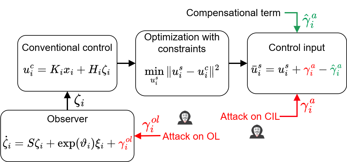
The SAAR control system is shown in Fig. 1. To address the attacks in (2), we finally design the following control input signal
| (19) | ||||
| (20) | ||||
| (21) |
where the compensational signal mitigates the adverse effects caused by the attack (the false data injected into the communication channel, on which the data transmitted from the controller to the actuator is carried) and , and is adaptively tuned by (21) with constant .
To facilitate the stability analysis, we define the follower-observer tracking error vector as
| (22) |
where . Define the observer containment error vector as
| (23) |
Theorem 1.
Proof: Note that the global form of (12) is
| (24) |
where . Based on Lemma 3, since is nonsingular , to prove that is UUB is equivalent to proving that is UUB. The vector form of in (10) is
| (25) |
where . The time derivative of in (24) is
| (26) |
We consider the following Lyapunov function candidate
| (27) |
The time derivative of along the trajectory of (26) is given by
| (28) |
For convenience, denote and , which are both positive constants. To let , we need
| (29) |
A sufficient condition to guarantee (29) is
| (30) |
A sufficient condition to guarantee (30) is and . From Assumption 4, , to prove that , we need to prove that . Based on (11), when , which guarantees the exponential growth of dominates all other terms, , such that , . Hence, we obtain ,
| (31) |
By LaSalle’s invariance principle [25], is UUB. Therefore, is UUB.
Next, we prove that follower-observer tracking error is UUB. From (1), (5), (10), (19) and (15), we obtain the time derivative of the elements in (22) as
| (32) |
From the above proof, we confirmed is UUB. Considering Assumption 2, (24) and (25), we obtain that is bounded. Let and . Note that is positive-definite. From (16), is symmetric positive-definite. Consider the following Lyapunov function candidate
| (33) |
and its time derivative is given by
| (34) |
Using (20) to obtain
| (35) |
To prove that , we need to prove that . Define , . Then, define the compact sets and . Considering Assumption 4, we obtain that . Hence, outside the compact set , , such that , ; outside the compact set , . Therefore, combining (34), (35) and (32), we obtain, outside the compact set , ,
| (36) |
Hence, by the LaSalle’s invariance principle, is UUB. We conclude that and are UUB, consequently, is UUB. Furthermore, based on Lemma 2, under the satisfaction of safety constraints (18), we obtain that . That is . This completes the proof.
IV Numerical Simulations
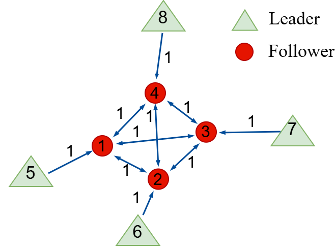
In this section, we validate the proposed SAAR control strategies through numerical simulations of a heterogeneous autonomous MAS under EU-FDI attacks on both CIL and OL. Fig. 2 illustrates the communication topology among the agents. As seen, the autonomous MAS consists of four followers (agent 1 to 4) and four leaders (agent 5 to 8), with the dynamics of the followers and the leaders modeled by the following equations:
We inject the following EU-FDI attack signals on the CIL and OL:
These attack signals, which grow exponentially over time, are crafted to evaluate the system’s ability to adapt and maintain resilience in the face of evolving adversarial conditions. Select , and . The controller gain matrices and are found by solving (14)-(16).
We choose for collision avoidance. The performance of the proposed SAAR control strategies, considering these safety constraints, is demonstrated through a set of comparative simulation results contrasted with non-SAAR standard control protocols [20]. The three sub-figures in Fig. 3 illustrate the initial three-dimensional (3D) positions of the agents and compare the system responses under standard control and SAAR control following the attacks. Both EU-FDI attacks on the OL and CIL are initiated at . Fig. 3(a) depicts the initial positions of the agents, while Fig. 3(b) presents the agents’ 3D positions at under the standard control approach, where the containment objective is not achieved post-attack. In contrast, Fig. 3(c) displays the agents’ 3D positions at under the SAAR control approach, demonstrating that the UUB containment objective is preserved despite the attacks.
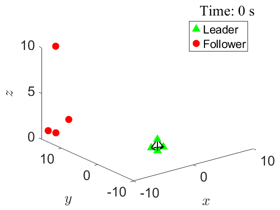
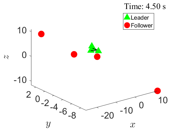
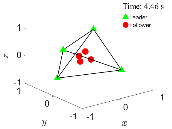
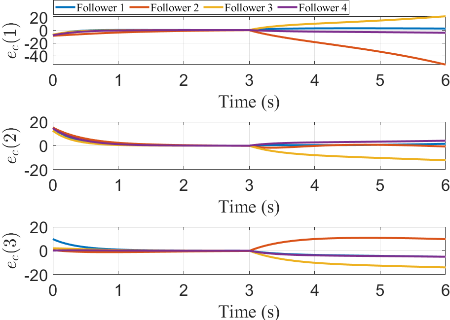
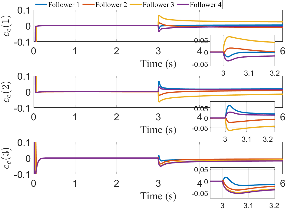
Fig. 4(a) illustrates the evolution of the containment error under conventional control. The dimensional components of diverge, indicating a failure in achieving containment. In contrast, Fig. 4(b) depicts the system response under SAAR control following the injection of the attacks. While brief spikes in the error reflect the system’s transient response to the attacks, the SAAR controller quickly compensates, causing the errors to stabilize and enter a steady state. This behavior demonstrates the resilience of the SAAR controller in maintaining UUB containment performance by effectively mitigating the impact of EU-FDI attacks on both CIL and OL.
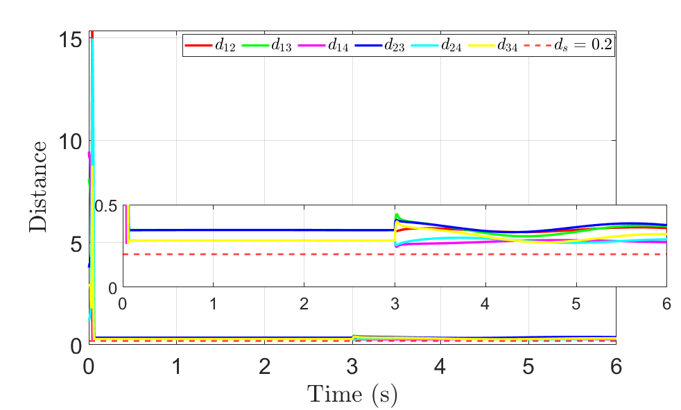
Fig. 5 depicts the evolution of the distances between followers, denoted as and , over time. Following the attacks, a brief spike in the distances is observed as the system experiences a transient response. However, the SAAR controller quickly compensates, and the distances stabilize shortly after, ensuring collision avoidance among followers. Fig. 4(b) and Fig. 5 show that the system successfully maintains safety and achieves the UUB containment under EU-FDI attacks on both OL and CIL, validating the effectiveness of the proposed SAAR defense strategies.
V Conclusion
In this study, we have developed a SAAR control framework to address the challenges posed by EU-FDI attacks on autonomous MASs. We have introduced an attack-resilient OL and integrated safety constraints through QP to achieve collision avoidance, ensuring system safety even under attack. Additionally, a compensational signal has been designed to counteract the impact of EU-FDI attacks on the CIL. Rigorous Lyapunov stability analysis and 3D simulations have demonstrated the SAAR controller’s effectiveness in maintaining both safety and resilience in practical autonomous MAS environments, where leader agents span safe regions to guide heterogeneous follower agents while addressing collision avoidance.
References
- [1] M. Petrlík, T. Báča, D. Heřt, M. Vrba, T. Krajník, and M. Saska, “A robust uav system for operations in a constrained environment,” IEEE Robotics and Automation Letters, vol. 5, no. 2, pp. 2169–2176, 2020.
- [2] J. He, Y. Zhou, L. Huang, Y. Kong, and H. Cheng, “Ground and aerial collaborative mapping in urban environments,” IEEE Robotics and Automation Letters, vol. 6, no. 1, pp. 95–102, 2020.
- [3] P. Weng, B. Chen, S. Liu, and L. Yu, “Secure nonlinear fusion estimation for cyber–physical systems under FDI attacks,” Automatica, vol. 148, p. 110759, 2023.
- [4] D. Zhang, Z. Ye, and X. Dong, “Co-design of fault detection and consensus control protocol for multi-agent systems under hidden dos attack,” IEEE Transactions on Circuits and Systems I: Regular Papers, vol. 68, no. 5, pp. 2158–2170, 2021.
- [5] F. Pasqualetti, F. Dörfler, and F. Bullo, “Attack detection and identification in cyber-physical systems,” IEEE transactions on automatic control, vol. 58, no. 11, pp. 2715–2729, 2013.
- [6] S. Zuo, Y. Wang, M. Rajabinezhad, and Y. Zhang, “Resilient containment control of heterogeneous multi-agent systems against unbounded attacks on sensors and actuators,” IEEE Transactions on Control of Network Systems, 2023.
- [7] S. Zuo and D. Yue, “Resilient containment of multigroup systems against unknown unbounded fdi attacks,” IEEE Transactions on Industrial Electronics, vol. 69, no. 3, pp. 2864–2873, 2021.
- [8] Y. Shi, Y. Hua, J. Yu, X. Dong, J. Lü, and Z. Ren, “Resilient output formation-containment tracking of heterogeneous multi-agent systems: A learning-based framework using dynamic data,” IEEE Transactions on Network Science and Engineering, 2024.
- [9] Z. Liao, S. Wang, J. Shi, S. Haesaert, Y. Zhang, and Z. Sun, “Resilient containment under time-varying networks with relaxed graph robustness,” IEEE Transactions on Network Science and Engineering, 2024.
- [10] W. Sun, Y. Zhang, Y. Yang, and S. Zuo, “Resilience-based output containment control of heterogeneous mas against unbounded attacks,” IET Control Theory & Applications, vol. 17, no. 6, pp. 757–768, 2023.
- [11] K. Garg, E. Arabi, and D. Panagou, “Fixed-time control under spatiotemporal and input constraints: A quadratic programming based approach,” Automatica, vol. 141, p. 110314, 2022.
- [12] M. H. Cohen, R. K. Cosner, and A. D. Ames, “Constructive safety-critical control: Synthesizing control barrier functions for partially feedback linearizable systems,” IEEE Control Systems Letters, 2024.
- [13] S. Wu, T. Liu, M. Egerstedt, and Z.-P. Jiang, “Quadratic programming for continuous control of safety-critical multiagent systems under uncertainty,” IEEE Transactions on Automatic Control, vol. 68, no. 11, pp. 6664–6679, 2023.
- [14] M. H. Cohen, P. Ong, G. Bahati, and A. D. Ames, “Characterizing smooth safety filters via the implicit function theorem,” IEEE Control Systems Letters, 2023.
- [15] X. Tan and D. V. Dimarogonas, “On the undesired equilibria induced by control barrier function based quadratic programs,” Automatica, vol. 159, p. 111359, 2024.
- [16] H. Ye, C. Wen, and Y. Song, “Decentralized and distributed control of large-scale interconnected multi-agent systems in prescribed time,” IEEE Transactions on Automatic Control, 2024.
- [17] D. Widder, Advanced Calculus: Second Edition. Dover Publications, 2012.
- [18] R. T. Rockafellar, “Convex analysis:(pms-28),” 2015.
- [19] H. Khalil, Nonlinear Systems, 3rd ed. Prentice Hall, 2002.
- [20] S. Zuo, Y. Song, F. L. Lewis, and A. Davoudi, “Output containment control of linear heterogeneous multi-agent systems using internal model principle,” IEEE transactions on cybernetics, vol. 47, no. 8, pp. 2099–2109, 2017.
- [21] A. D. Ames, J. W. Grizzle, and P. Tabuada, “Control barrier function based quadratic programs with application to adaptive cruise control,” in 53rd IEEE conference on decision and control. IEEE, 2014, pp. 6271–6278.
- [22] K. Garg and D. Panagou, “Distributed robust control synthesis for safety and fixed-time stability in multi-agent systems,” arXiv preprint arXiv:2004.01054, 2020.
- [23] J. Huang, Nonlinear output regulation: theory and applications. SIAM, 2004.
- [24] J. Zhang, L. Ding, X. Lu, and W. Tang, “A novel real-time control approach for sparse and safe frequency regulation in inverter intensive microgrids,” IEEE Transactions on Industry Applications, 2023.
- [25] M. Krstic, P. V. Kokotovic, and I. Kanellakopoulos, Nonlinear and adaptive control design. John Wiley & Sons, Inc., 1995.