2 OLMo 2 Furious

Abstract

We present OLMo 2, the next generation of our fully open language models. OLMo 2 includes dense autoregressive models with improved architecture and training recipe, pretraining data mixtures, and instruction tuning recipes. Our modified model architecture and training recipe achieve both better training stability and improved per-token efficiency. Our updated pretraining data mixture introduces a new, specialized data mix called Dolmino Mix 1124, which significantly improves model capabilities across many downstream task benchmarks when introduced via late-stage curriculum training (i.e. specialized data during the annealing phase of pretraining). Finally, we incorporate best practices from Tülu 3 to develop OLMo 2-Instruct, focusing on permissive data and extending our final-stage reinforcement learning with verifiable rewards (RLVR). Our OLMo 2 base models sit at the Pareto frontier of performance to compute, often matching or outperforming open-weight only models like Llama 3.1 and Qwen 2.5 while using fewer FLOPs and with fully transparent training data, code, and recipe. Our fully open OLMo 2-Instruct models are competitive with or surpassing open-weight only models of comparable size, including Qwen 2.5, Llama 3.1 and Gemma 2. We release all OLMo 2 artifacts openly—models at 7B and 13B scales, both pretrained and post-trained, including their full training data, training code and recipes, training logs and thousands of intermediate checkpoints. The final instruction model is available on the Ai2 Playground as a free research demo.

[  OLMo 2 Base:]OLMo-2-1124-7B  OLMo-2-1124-13B [  OLMo 2 Instruct:] OLMo-2-1124-7B-Instruct  OLMo-2-1124-13B-Instruct [  Base Data:] olmo-mix-1124 (pretrain)  dolmino-mix-1124 (midtrain) [  Instruct Data:] tulu-3-sft-olmo-2 (sft)  olmo-2-1124-{7b|13b} (dpo)  tulu-3-rlvr (rlvr) [  Training Code:] OLMo (pretrain v1)  OLMo-core (pretrain v2)  open-instruct (posttrain) [  Eval & Data Code:] olmes (eval suite)  dolma (data curation) [  WandB Logs:] 7B  13B [  Demo:]playground.allenai.org [  Contact:]olmo@allenai.org

Figure 1: Performance to pretraining FLOPs ($\approx$ 6 $\times$ training tokens $\times$ model size; Kaplan et al., 2020) for OLMo 2 and comparable models. We see that the fully open OLMo 2 lies on the Pareto frontier, outperforming many other models of varying levels of openness at multiple sizes. For full results, see Table 6.

1 Introduction

The open language model ecosystem has grown rapidly in the past year, with open weights models—from established and new contributors—substantially closing the gap between publicly available and closed systems (Cottier et al., 2024). Yet, these open-weights models are only the final artifacts of sophisticated language model recipes and complex development pipelines, and by themselves are not sufficient to support diverse forms of research into language model behaviors and uses. The first iteration of OLMo (Groeneveld et al., 2024)—alongside EleutherAI’s Pythia (Biderman et al., 2023) and LLM-360 Amber (Liu et al., 2023b)—adopted a fully open approach, releasing not just model weights but also training data, code, recipes and more. This approach has been since followed by AI builders from DCLM (Li et al., 2024), Multimodal Art Projection (M-A-P) (Zhang et al., 2024a), and HuggingFace (Allal et al., 2024a, b). OLMo artifacts have played a crucial role in studying training dynamics (Land and Bartolo, 2024; Jin and Ren, 2024), concept acquisition (Chang et al., 2024), and memorization (Antoniades et al., 2024; Shaib et al., 2024) in language models; further, they have lead to the creation of techniques (Vyas et al., 2024; Zhao et al., 2024) and models (Tokpanov et al., 2024; Liu et al., 2024; Shao et al., 2024).

Modern language model development is an iterative process, whereby limitations of current iterations motivate future development. Our previous release (OLMo-0424; Ai2, 2024) focused on improving performance on key tasks (e.g., MMLU) through better pretraining data mixing and curricula. In this technical report, we introduce OLMo 2, a new family of 7B and 13B models trained on up to 5T tokens. On English academic benchmarks, these models are on par with or better than equivalently-sized fully open models, and are competitive with the open weight Llama 3.1 and Qwen 2.5 families of models (Figure 1). This technical report focuses on four key areas we targeted during development of OLMo 2:

• Pretraining Stability. Language model training runs are often plagued by training instabilities and loss spikes, which are costly and known to be a detriment to final model performance. We discuss techniques we used to improve training stability, which was critical to ensuring performance of the final trained model (Section §3).

• Mid-training Recipe. OLMo-0424 (Ai2, 2024), DBRX (Databricks, 2024), and Llama 3 (Grattafiori et al., 2024) demonstrated the usefulness of data curricula for pretraining, as discussed by Blakeney et al. (2024). We discuss the advantages of splitting pretraining into two stages, with the latter mid-training stage being used to infuse new knowledge and patch deficiencies in capabilities. Further, we show how data sources for mid-training can be independently assessed to reduce experimentation cost through a technique we call micro-annealing (Section §4).

• Post-training Pipeline. A key deliverable for a successful base model is its ability to be finetuned to downstream use-cases. We introduce OLMo 2-Instruct built on the Tülu 3 recipe (Lambert et al., 2024), and show how improvements in base models translated to better chat variants. We focus on permissive data and expand the reinforcement learning with verifiable rewards (RLVR) pipeline to multiple stages for maximum performance (Section §5).

• Infrastructure as a Research Catalyst. High performance and reliable infrastructure is crucial for successful pretraining; yet, many pretraining papers do not discuss their training stack, or gloss over crucial details. We discuss changes from OLMo-0424 that enable the improvements of OLMo 2, and how investing in solutions that let us monitor and orchestrate infrastructure helped us reduce failure rates and increase cluster utilization (Section §6).

Alongside these deep dives, we provide a description of the full model development procedure in Section §2: training data, pretraining, post-training, and evaluation. We highlight changes from OLMo 1 and OLMo-0424 when appropriate, and reference related projects, such as our scaling laws effort to efficiently estimate model downstream performance (Bhagia et al., 2024) and benchmark standardization through the OLMES evaluation framework (Gu et al., 2024).

2 OLMo 2 Family

This section provides an overview of OLMo 2 and highlights improvements over OLMo-0424 and previous OLMo models. The OLMo 2 family has more tokens, more parameters, and has better downstream task results compared to OLMo-0424. We explain the crucial details required to achieve competitive results in our mission of making state-of-the-art language models accessible. Accordingly, we release all training code, data, and recipes openly under the Apache 2.0 license wherever possible, and under the most permissive available license otherwise.

2.1 Base Model Data

Following previous OLMo models, as well as recent advances in curriculum learning (Blakeney et al., 2024; Ibrahim et al., 2024), base OLMo 2 models are trained in two stages, each with its corresponding data mix. The first pretraining stage is the longest ($\geqslant 90\%$ training FLOPs), and uses mostly web-sourced data. In this stage, we use an iteration on our pretraining mix of high-quality web data drawing on other recent open data releases. During the second stage, which we refer to as mid-training ($5\textup{--}10\%$ of training FLOPs), we up-sample the highest-quality web documents and curated non-web sources; we also employ synthetic data crafted to patch math capabilities of the model.

We provide a brief overview of data mix for pretraining and mid-training in the reminder of this section; we spent considerable efforts on developing a methodology to curate mid-training data, which we present in a deep dive in Section §4. In total, OLMo 2 7B is trained on $4.05$ trillion tokens ($3.90$ trillion for pretraining stage), while OLMo 2 13B is trained on $5.6$ trillion tokens ($5$ trillion for pretraining stage).

2.1.1 Pretraining data: OLMo 2 Mix 1124

Source	Type	Tokens	Words	Bytes	Docs
Pretraining ✦ OLMo 2 1124 Mix
DCLM-Baseline	Web pages	3.71T	3.32T	21.32T	2.95B
StarCoder       filtered version       from OLMoE Mix	Code	83.0B	70.0B	459B	78.7M
peS2o       from Dolma 1.7	Academic papers	58.6B	51.1B	413B	38.8M
arXiv	STEM papers	20.8B	19.3B	77.2B	3.95M
OpenWebMath	Math web pages	12.2B	11.1B	47.2B	2.89M
Algebraic Stack	Math proofs code	11.8B	10.8B	44.0B	2.83M
Wikipedia & Wikibooks       from Dolma 1.7	Encyclopedic	3.7B	3.16B	16.2B	6.17M
Total		3.90T	3.48T	22.38T	3.08B

Table 1: Composition of the pretraining data for OLMo 2. The OLMo 2 1124 Mix is composed of StarCoder (Li et al., 2023b; Kocetkov et al., 2022), peS2o (Soldaini and Lo, 2023), web text from DCLM (Li et al., 2024) and Wiki come from Dolma 1.7 (Soldaini et al., 2024). arXiv comes from Red-Pajama (Together AI, 2023), while OpenWebMath (Paster et al., 2023) and Algebraic Stack come from ProofPile II (Azerbayev et al., 2023).

The mix used for this stage is shown in Table 1. It consists of approximately 3.9 trillion tokens, with over 95% derived from web data. We refer to this set as OLMo 2 Mix 1124. This is the same pretraining data used in OLMoE (Muennighoff et al., 2024).

We combine data from DCLM (Li et al., 2024) and Dolma 1.7 (Soldaini et al., 2024). From DCLM, we use the “baseline 1.0” mix. From Dolma, we use the arXiv (Together AI, 2023), OpenWebMath (Paster et al., 2023), Algebraic Stack, peS2o (Soldaini and Lo, 2023), and Wikipedia subsets. arXiv, OpenWebMath, and Algebraic Stack were originally part of ProofPile II (Azerbayev et al., 2023).

Finally, we include code from StarCoder (Li et al., 2023b), which is derived from permissively-licensed repositories from GitHub (Kocetkov et al., 2022). In an attempt to include higher quality code, we remove any document from a repository with fewer than 2 stars on GitHub. Further, through manual inspection of this source, we found it to contain documents encoded in binary format or containing mostly numerical content; to remove them, we discarded documents whose most frequent word constitutes over 30% of the document, or whose top-2 most frequent words constitute over 50% of the document. To mitigate possible training loss spikes, we remove documents with repeated sequences of 32 or more n-grams. We report details and show effectiveness of this intervention in Section §3.1.

2.1.2 Mid-training data: Dolmino Mix 1124

Source	Type	Tokens	Words	Bytes	Docs
Mid-Training ✦ Dolmino High Quality Subset
DCLM-Baseline       FastText top 7%       $\text{FineWeb}\geqslant 2$	High quality web	752B	670B	4.56T	606M
FLAN       from Dolma 1.7       decontaminated	Instruction data	17.0B	14.4B	98.2B	57.3M
peS2o       from Dolma 1.7	Academic papers	58.6B	51.1B	413B	38.8M
Wikipedia & Wikibooks       from Dolma 1.7	Encyclopedic	3.7B	3.16B	16.2B	6.17M
Stack Exchange       09/30/2024 dump       curated Q&A data	Q&A	1.26B	1.14B	7.72B	2.48M
High quality total		832.6B	739.8B	5.09T	710.8M
Mid-training ✦ Dolmino Math Mix
TuluMath	Synthetic math	230M	222M	1.03B	220K
Dolmino SynthMath	Synthetic math	28.7M	35.1M	163M	725K
TinyGSM-MIND	Synthetic math	6.48B	5.68B	25.52B	17M
MathCoder2 Synthetic       Ajibawa-2023       M-A-P Matrix	Synthetic Math	3.87B	3.71B	18.4B	2.83M
Metamath       OWM-filtered	Math	84.2M	76.6M	741M	383K
CodeSearchNet       OWM-filtered	Code	1.78M	1.41M	29.8M	7.27K
GSM8K       Train split	Math	2.74M	3.00M	25.3M	17.6K
Math total		10.7B	9.73B	45.9B	21.37M

Table 2: Composition of the mid-training data (Dolmino). From this set, we create samples of 50B, 100B and 300B tokens to mid-train OLMo 2 on. See Section §4 for details regarding individual source details, and Table 13 for the specific composition of each annealing mixture.

After the initial pretraining stage on mostly web data, we further train with a mixture of web data that has been more restrictively filtered for quality and a collection of domain-specific high quality data, much of which is synthetic. The purpose of this mixture is to imbue the model with math-centric skills and provide focused exposure to STEM references and high quality text. We generate several variants of this mixture, with varying sizes, but generally refer to this mixture as Dolmino Mix 1124. The base sources from which Dolmino Mix 1124 is subsampled are described in Table 2. We refer the reader to Section §4 for a deep dive detailing our processes for experimenting and curating data for this mix.

2.2 Model Architecture

	OLMo 1 (0224)	OLMo-0424	OLMo 2
Biases	None	None	None
Activation	SwiGLU	SwiGLU	SwiGLU
RoPE $\theta$	$1\cdot 10^{4}$	$1\cdot 10^{4}$	$5\cdot 10^{5}$
QKV Normalization	None	Clip to $8$	QK-Norm
Layer Norm	non-parametric	non-parametric	RMSNorm
Layer Norm Applied to	Inputs	Inputs	Outputs
Z-Loss Weight	$0$	$0$	$10^{-5}$
Weight Decay on Embeddings	Yes	Yes	No

Table 3: Summary of how OLMo family model architectures have evolved over time. Latest OLMo 2 changes were motivated by experiments showing improved training stability. Full descriptions in §2.2.

Table 3 provides an overview of how the model architecture has evolved through iterations in the OLMo family. We provide details below:

We adopt a decoder-only transformer architecture based on Vaswani et al. (2017), and deliver 7B and 13B parameter variants as described in Table 4. Our architecture is very similar to the first iteration of OLMo (Groeneveld et al., 2024), with several changes to improve training stability (see Section §3) and performance. The original OLMo modified the decoder-only transformer architecture (Vaswani et al., 2017) with:

• No biases: We exclude all bias terms from our architecture (Groeneveld et al., 2024; Chowdhery et al., 2022, inter alia).

• SwiGLU activation function: We use the SwiGLU activation function (Shazeer, 2020) and set the corresponding hidden size to approximately $\frac{8}{3}d$, but increased to the closest multiple of 128 ($11,008$ for our 7B model) to improve throughput.

• Rotary positional embeddings (RoPE): We replace absolute positional embeddings with rotary positional embeddings (RoPE; Su et al., 2021).

When building OLMo-0424, we made modifications for training stability and downstream performance:

• QKV Clipping: For training stability, also as seen in DBRX (Databricks, 2024).

• Increased context: From 2048 to 4096.

Finally, this work introduces OLMo 2 which made further modifications:

• RMSNorm: We use the RMSNorm (Zhang and Sennrich, 2019) variant of LayerNorm (Ba et al., 2016) without a bias term to normalize activations, instead of nonparametric LayerNorm.

• Reordered norm: We normalize the outputs to the attention and feedforward (MLP) layers within each transformer block, instead of the inputs. So the formula for each block becomes:

  $$\boldsymbol{h}:=\boldsymbol{x}+\text{RMSNorm}(\text{Attention}(\boldsymbol{x}))$$ (1)

  $$\boldsymbol{h}_{\text{out}}:=\boldsymbol{h}+\text{RMSNorm}(\text{MLP}(\boldsymbol{x}))$$ (2)

  where $\boldsymbol{x}$ is the input to the layer, $\boldsymbol{h}$ is an intermediate hidden state, and $\boldsymbol{h}_{\text{out}}$ is the output. This strategy was first proposed by Liu et al. (2021) to stabilize training.

• QK-norm: Following Dehghani et al. (2023b) we normalize the key and query projections with RMSNorm before calculating attention. This avoids attention logits being too large, which can lead to training loss divergence.

• Z-Loss: Following Chowdhery et al. (2022), Chameleon Team (2024), and Wortsman et al. (2023), we adopt z-loss regularization, as it has been empirically shown to improve run stability.

• RoPE $\boldsymbol{\theta=5e5}$: We increase the RoPE $\theta$ to 500,000 from 10,000. This approach increases the resolution of positional encoding, matching Grattafiori et al. (2024).

2.3 Pretraining Recipe

	OLMo 2 7B	OLMo 2 13B
Layers	32	40
Hidden Size $(d_{model})$	4096	5120
Attention Heads	32	40
Batch Size	1024	2048
Sequence Length	4096	4096
Gradient Clipping	1.0	1.0
Peak Learning Rate	$3.0\cdot 10^{-4}$	$9.0\cdot 10^{-4}$
Learning Rate Warmup	2000 steps	2000 steps
Learning Rate Schedule	Cosine decay over 5T tokens (truncated after 4T)	Cosine decay over 5T tokens

Table 4: OLMo 2 hyperparameters.

As previously mentioned, we follow a two-stage procedure to train OLMo 2 base models.

Pretraining stage

Departing from previous OLMo versions, OLMo 2 models are randomly initialized from a truncated normal distribution with a mean of 0 and a standard deviation of 0.02 (see section 3.2). After that, we run a learning rate schedule that warms up the learning rate from 0 to the peak learning rate (a hyperparameter) over 2000 steps, followed by a cosine decay calibrated to reach 10% of the peak learning rate after 5T tokens. For the 7B variant, we truncate the schedule at 4T tokens and then begin the second stage. As the 13B variant ran with a higher learning rate from the start, we finish the cosine decay at 5T tokens before starting the second stage. In this stage, we train on broadly web-based data (see Table 1).

Mid-training stage

In the second stage, we train on the Dolmino Mix 1124 (Section §4). This mix is smaller, but contains higher-quality text, as well as synthetic data to boost key abilities with substantial room for improvement after the pretraining stage. For example, early versions of the OLMo 2 model underperformed on GSM8K relative to peer models, so we curated new data to target this. In this stage, we linearly decay the learning rate to zero over the length of the run.

To get the most out of this high-quality data, and to find a better local minimum, we perform this step multiple times with different random data orders, and then average the resulting models (Wortsman et al., 2022). For the 7B variant, we anneal three separate times for 50B tokens each, with different randomized data orders; we average the resulting models to produce the final model. For the 13B variant, we train three separate times for 100B tokens each (same number of update steps as the 7B), and then a fourth time for 300B tokens. The final model is the average of all four models. For further details, refer to Section §4.

2.3.1 Tokenizer

OLMo 1 and OLMo-0424 were trained using a modified version of the GPT-NeoX-20B tokenizer (Black et al., 2022) that includes special tokens ||| PHONE_NUMBER|||, |||EMAIL_ADDRESS|||, and |||IP_ADDRESS|||, which were used to mask personal identifiable information.

As suggested by Tao et al. (2024), we employ a larger tokenizer vocabulary for OLMo 2. We borrow pre-tokenizer and vocabulary from cl100k, the tokenizer developed for GPT-3.5 (OpenAI, 2023a) and GPT-4 (OpenAI, 2023b), which is licensed under Apache 2.0. To maintain backwards compatibility with early Dolma data sources, we add the same masking tokens used in previous OLMo models.

Tokenizer	OLMES (CF)	OLMES Gen	MMLU (CF)
OLMo 1 tokenizer	59.8	42.4	34.8
OLMo 2 tokenizer	60.6	42.7	35.2

Table 5: Comparison of OLMo 1 and OLMo 2 tokenizers on a 1B model pretrained for 100B tokens from DCLM baseline. Following Gu et al. (2024), OLMES and MMLU use CF format, which is more informative for small models.

We compare the two tokenizers at a smaller scale in Table 5. We see measurable gains when switching to the new tokenizer, particularly in OLMES tasks. Per Tao et al. (2024), at this model size and compute budget, the larger OLMo 2 tokenizer is at a slight disadvantage; we expect improvement coming from larger vocabulary to be more decisive at larger scales and for models trained on more tokens.

2.4 Base Model Evaluation

		Dev Benchmarks							Held-out Evals
Model	Avg	FLOP$\times 10^{23}$	MMLU	$\textbf{\leavevmode\nobreak\ ARC}_{\textbf{\leavevmode\nobreak\ C}}$	HSwag	WinoG	NQ	DROP	AGIEval	GSM8K	$\textbf{\leavevmode\nobreak\ MMLU}_{\textbf{\leavevmode\nobreak\ PRO}}$
Open-weight models
Llama 2 13B	51.0	1.6	55.7	67.3	83.9	74.9	38.4	45.6	41.5	28.1	23.9
Mistral 7B	56.6	n/a	63.5	78.3	83.1	77.7	37.2	51.8	47.3	40.1	30.0
Llama 3.1 8B	59.7	7.2	66.9	79.5	81.6	76.6	33.9	56.4	51.3	56.5	34.7
Mistral Nemo 12B	64.9	n/a	69.5	85.2	85.6	81.5	39.7	69.2	54.7	62.1	36.7
Gemma 2 9B	66.3	4.4	70.6	89.5	87.3	78.8	38.0	63.0	57.3	70.1	42.0
Qwen 2.5 7B	67.2	8.2	74.4	89.5	89.7	74.2	29.9	55.8	63.7	81.5	45.8
Qwen 2.5 14B	71.5	16.0	79.3	94.0	94.0	80.0	37.3	51.5	71.0	83.4	52.8
Models with partially available data
StableLM 2 12B	60.2	2.9	62.4	81.9	84.5	77.7	37.6	55.5	50.9	62.0	29.3
Zamba 2 7B	63.7	n/c	68.5	92.2	89.4	79.6	36.5	51.7	55.5	67.2	32.8
Fully-open models
Amber 7B	32.5	0.5	24.7	44.9	74.5	65.5	18.7	26.1	21.8	4.8	11.7
OLMo 7B	35.4	1.0	28.3	46.4	78.1	68.5	24.8	27.3	23.7	9.2	12.1
MAP Neo 7B	47.9	2.1	58.0	78.4	72.8	69.2	28.9	39.4	45.8	12.5	25.9
OLMo 0424 7B	49.8	1.0	54.3	66.9	80.1	73.6	29.6	50.0	43.9	27.7	22.1
DCLM 7B	55.2	1.0	64.4	79.8	82.3	77.3	28.8	39.3	47.5	46.1	31.3
OLMo 2 7B	61.2	1.8	63.7	79.8	83.8	77.2	36.9	60.8	50.4	67.5	31.0
OLMo 2 13B	66.8	4.6	67.5	83.5	86.4	81.5	46.7	70.7	54.2	75.1	35.1

Table 6: Evaluations comparing OLMo 2 to other base models on a subset of the OLMES suite (full suite details and results in Appendix A). Training FLOPs are computed using the approximation from Kaplan et al. (2020) and expressed as powers of $10^{23}$. We could not estimate compute for any Mistral model (Jiang et al., 2023; Mistral AI, 2024) because their total training token count is unknown. Training FLOPs for Zamba 2 (Glorioso et al., 2024) are not reported due to difference in architecture. Qwen 2.5 models (Qwen et al., 2024) are trained on a “maximum of 18 trillion tokens”; developers have declined to disclose exact token counts for each model size. OLMo 2 models were not evaluated on held-out datasets prior to release; we note that, for other models, we cannot guarantee the same.

We evaluate OLMo 2 on a mixture of multiple-choice and generative tasks. We use OLMES to assess performance of language models (Gu et al., 2024). OLMES is a set of principles and associated standard (with a reference implementation in the OLMES software framework) for reproducible LM evaluations that is open, practical, and documented, providing recommendations guided by experiments and results from the literature (Biderman et al., 2024; Gao et al., 2023). We provide an overview of OLMES in this section, and report results on a representative subset in Table 6; for more details, we refer the reader to Appendix A and Gu et al. (2024).

During model development, we considered a total of ten multiple-choice and five generative tasks. For multiple-choice tasks, we use the OLMES standard as introduced by OLMES. It is designed to support comparisons between smaller base models that require the cloze/completion formulation of multiple-choice questions (score each answer completion separately) against larger models that can handle the multiple-choice formulation. For all tasks, it uses a standardized prompt format and five in-context shots. Results for all OLMES tasks are reported in Appendix A.

Following the principles of OLMES, we also evaluated on a suite of five generative tasks (OLMES-Gen). This suite covers factual knowledge tasks (Natural Questions, Kwiatkowski et al., 2019, reported in Table 6) and tasks testing reading comprehension (DROP, Dua et al., 2019, reported in Table 6). We use F1 as the primary metric to give partial credit when models produce answers that partially match. The task details of OLMES-Gen are summarized in Table 20. Evaluation results on the generative tasks are given in Table 22 in Appendix D.

Finally, we also consider a held-out suite of tasks that were not used when making decisions during model development. A subset consisting of AGIEval (Zhong et al., 2024), GSM8K (Cobbe et al., 2021), and MMLU Pro (Wang et al., 2024) is reported in Table 6. For the rest, we refer to the reader to Appendix A. Note that for the case of GSM8K, we never evaluated our models on the entire test set during development: instead, we use 200 examples to inform choices (e.g., choices of annealing mixtures). In §4.1 we refer to this 200-example subset as “GSM*.” Evaluation results on the held-out tasks can be found in Table 23 in Appendix D.

Overall, we find that gains observed on development metrics largely translate to our unseen evaluation suite. Of course, we have no guarantee that tasks we consider unseen during development of OLMo 2 are not part of the development set of other models we compare. Nevertheless, we think it should be standard practice for model developers to keep a subset of evaluation tasks unseen and to declare which these are, in technical reports. Further, we encourage other open-weight model developers to clearly state which tasks are being monitored during model development.

2.5 Post-Training Recipe and Evaluation

For post-training we follow the Tülu 3 recipe with diverse, skill-centric supervised finetuning data, on-policy preference data, and reinforcement learning with verifiable rewards (RLVR) (Lambert et al., 2024). We created new preference data from permissively licensed model outputs and added a multi-stage RLVR training protocol to optimize final performance. The OLMo 2-Instruct models are evaluated in Table 7 on general and precise instruction following, math, knowledge reasoning, and safety tasks. Full post training details are in Section §5.

Instruct Model	AVG	AE2	BBH	DROP	GSM8K	IFE	MATH	MMLU	Safety	PQA	TQA
Open weights models
Ministral 8B 2410	53.5	31.4	70.8	56.2	80.0	56.4	40.0	68.5	56.2	20.2	55.5
Llama 3.1 8B	59.1	25.8	71.9	61.7	83.4	80.6	42.5	71.3	70.2	28.4	55.1
Tulu 3 8B	60.7	34.0	69.0	62.6	87.6	82.4	43.7	68.2	75.4	29.1	55.0
Qwen 2.5 7B	61.6	29.7	70.2	54.4	83.8	74.7	69.9	76.6	75.0	18.1	63.1
Gemma 2 9B	58.1	43.7	64.9	58.8	79.7	69.9	29.8	69.1	75.5	28.3	61.4
Qwen 2.5 14B	65.2	34.6	78.4	50.5	83.9	82.4	70.6	81.1	79.3	21.1	70.8
Fully-open models
OLMoE 1B 7B 0924	35.5	8.5	37.2	34.3	47.2	46.2	8.4	51.6	51.6	20.6	49.1
OLMo 7B 0724	34.3	9.4	39.2	44.9	23.7	37.7	4.9	51.6	53.6	18.2	59.2
OLMo 2 7B	55.2	29.1	51.4	60.5	85.1	72.3	32.5	61.3	80.6	23.2	56.5
OLMo 2 13B	62.4	39.5	63.0	71.5	87.4	82.6	39.2	68.5	79.1	28.8	64.3

Table 7: The results for OLMo 2 Instruct at both 7B and 13B relative to peer open weight models. The following evaluation names are abbreviated: AVG – Average, AE2 – AlpacaEval 2, BBH – BigBenchHard, IFE – IFEval, PQA – PopQA, TQA – TruthfulQA. All models in this table are the instruction tuned variants.

3 Deep Dive: Pretraining Stability

While OLMo-0424 achieved performance within expected ranges for its compute budget, the training dynamics were characterized by a couple of concerns:

• Sudden spikes in the loss, and more frequently, in the gradient norm during training. In experiments, we found that increasing model size increased the frequency of spikes. Furthermore, our experiments revealed that more dramatic spikes in gradient norm often preceded training loss spikes.

• Slow growth in the magnitude of the gradient norm over the training run. This was correlated with increasing frequency of spikes in the gradient norm (and training loss).

Figure 2: Training loss and gradient norm curves (over training steps) for OLMo-0424 and OLMo 2. The OLMo-0424 training run was characterized by frequent loss spikes (top), often preceded by more frequent spikes in the gradient norm, which grew over time (bottom). We note that overall training loss for OLMo 2 is higher because the underlying training data changed between the runs.

Ultimately, a combination of these issues would lead to training divergence, making training at larger scales impossible. This situation motivated our training stability investigation into the causes of these issues and their mitigations. Figure 2 shows our training curves before and after implementing our mitigations, which we summarize below:

• Repeated n-grams: We filter pretraining data to remove repeated n-grams in pretraining data, as they can lead to loss spikes (§3.1).

• Initialization: We switch from scaled initialization (Zhang et al., 2019) to initializing all parameters with a mean of 0 and a standard deviation of 0.02 (§3.2).

• RMSNorm: We use the RMSNorm variant of LayerNorm to normalize activations instead of non-parametric LayerNorm (§3.3.2).

• Reordered norm: We normalize the outputs to the attention and feed-forward (MLP) layers within each transformer block instead of the inputs (§3.3.2).

• QK-norm: We normalize the key and query projections with RMSNorm before calculating attention (§3.3.2).

• Z-Loss: We adopt z-loss regularization, a regularization term that keeps final output logits from growing too large (§3.3.3).

• Weight decay: We exclude embeddings from weight decay (§3.4.2).

• $\epsilon$ in AdamW: We lower the $\epsilon$ of AdamW from $10^{-5}$ to $10^{-8}$ (§3.4.1).

In the following, we will discuss the experiments and results that led us to these interventions. We compare our revised strategies with OLMo-0424, the most recent version of OLMo with fully-open model weights, data, and documentation.

3.1 Repeated n-Grams

Data can be a cause of both gradient norm and loss spikes. When investigating training batches at which spikes occurred, we found a high prevalence of instances containing long, repeated n-gram sequences. Here are three examples of such sequences:

      g4ODg4ODg4ODg4ODg4ODg4ODg4ODg4ODg4ODg4ODg4ODg4ODg4ODg4OD...
      [\n  365, 0, 667, 1000, 1000, 667, 667, 667, 667, 667, ...
      ’ 255, 255, 255, 255, 255, 255, 255, 255, \n255, 255, ...

In a series of experiments, we found these sequences are often associated with spikes, though we note that this relationship is not deterministic:

• The same n-gram sequence may spike for a larger model but not for a smaller model trained on the same data.

• The same n-gram sequence may spike for one data training ordering, but not after the data is reshuffled.

• The same n-gram sequence associated with a spike can also be found elsewhere in training batches that did not spike.

Figure 3: Comparison of the gradient norm for two runs, one without n-gram filter, and one with. Ignoring long repetitive sequences of n-grams eliminates many spikes.

Nevertheless, we have found evidence that broad removal of such sequences across training decreases the frequency of spikes, on average. At data curation time (Section §2.1), we apply a filter that removes all documents with a sequence of 32 or more repeated n-grams, where an n-gram is any span of 1 to 13 tokens. We also implement an additional safe-guard in the trainer that detects these sequences during data loading and masks them when computing the loss. Figure 3 shows the effect of masking the loss of input sequences containing repeated n-grams. This intervention results in a clear mitigation—though not complete elimination—of gradient spikes. It had no effect on the slow growth in gradient norm.

3.2 Model Initialization

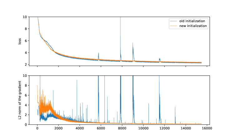
Figure 4: In our test setting, the OLMo-0424 initialization scheme shows instabilities quickly, while OLMo 2 stays stable.

Figure 4 shows the improvement to training stability from OLMo 2’s initialization scheme. In OLMo 2, we initialize every parameter from a normal distribution with a mean of 0 and a standard deviation of 0.02. In contrast, OLMo-0424’s initialization, first suggested in Zhang et al. (2019) and implemented by Gururangan et al. (2023), scaled input projections by $1/\sqrt{d_{\mathrm{model}}}$, and output projections by $1/\sqrt{2\cdot d_{\mathrm{model}}\cdot\mathrm{layer\_idx}}$ at every layer. In other words, later layers were initialized to smaller values.

We perform several analyses to study the impact of initialization, showing that OLMo 2’s initialization is superior to OLMo-0424 initialization. Our empirical analysis suggests it better preserves the scale of activations and gradients across layers, allowing deep models to be trained more stably, and it exhibits properties associated with hyperparameter transfer across models of different widths. These two properties together give us confidence that deep models will train stably and that the initialization hyperparameters of our smaller models could transfer to larger scales.

Gradient and activation growth

A fundamental concern for training deep networks is ensuring that the activations and gradients do not blow up or vanish across layers, causing learning to become unstable or stagnate. Rather, we want the scale of the activations and gradients to remain roughly the same from layer to layer. Inspired by recent related work (Cowsik et al., 2024), we evaluate different candidate initializations in terms of how they affect the 2-norm of the activations and gradients across layers. Concretely, we randomly initialize a model, pass 50 random documents from The Pile (Gao et al., 2021) through it, and collect the activations and gradients (of loss with respect to the activations) at the initial and final layers (ignoring embeddings). We then average these tensors across documents and time steps to get vectors $\boldsymbol{v}$ at the initial layer and $\boldsymbol{v^{\prime}}$ at the final layer, both of length $d_{\mathrm{model}}$. Finally, we compute the following measure of expansion or contraction across layers, which we call the growth exponent:

$$\lambda=\frac{1}{n_{\mathrm{layers}}}\log\left(\frac{\left\lVert\boldsymbol{v^{\prime}}\right\rVert}{\left\lVert\boldsymbol{v}\right\rVert}\right)$$

We compute $\lambda$ for both the activations and gradients. Ideally, both $\lambda$’s remain near 0, indicating that the activations and gradients do not explode or vanish across layers. Figure 5 plots the growth exponents for different randomly initialized models as a function of their widths (4096 corresponds to a full 7B model). Crucially, the growth exponent for OLMo 2 is closer to 0 than for OLMo-0424 across model widths. This suggests the OLMo 2 initialization will be more stable when training deep models in low precision, as both the activations and the gradients are more resistant to exploding or vanishing across layers compared to the original OLMo-0424 initialization.

Hyperparameter transfer across width

Another appealing property of the new initialization is that it scales the activation and gradient norms with width ($d_{\mathrm{model}}$) in a way that has been argued theoretically to be important for hyperparameter transfer across different widths. Specifically, Yang et al. (2024b) suggest that a sufficient condition for hyperparameter transfer across width is that the magnitude of each activation scalar value and its update (learning rate times gradient) remain fixed as width increases. Equivalently, the norms of the activations and their update vectors should positively correlate with $\sqrt{d_{\mathrm{model}}}$. We plot the activation and gradient norms at initialization against $\sqrt{d_{\mathrm{model}}}$ in Figure 6. Crucially, the gradient norm is more positively correlated with $\sqrt{d_{\mathrm{model}}}$ for OLMo 2 compared to OLMo-0424. Combined with Yang et al. (2024b), this suggests that, with an initial learning rate independent of model width, the new OLMo 2 initialization will transfer better across different model widths compared to the OLMo-0424 initialization.

Figure 5: Across widths, growth exponents for the OLMo 2 initialization are closer to 0 compared to the OLMo-0424 initialization, which suggests deeper models will train more stably.

Figure 6: Activation and gradient norms vs. $\sqrt{d_{\mathrm{model}}}$ for the OLMo-0424 and OLMo 2 initializations. Crucially, the gradient norms for OLMo 2 positively correlate with $\sqrt{d_{\mathrm{model}}}$, which they did not for the OLMo-0424 initialization. This suggests the OLMo 2 initialization will show better hyperparameter transfer across widths (Yang et al., 2024b).

Spike score

Since fast spikes are difficult to understand with contemporary graphing tools, we compute a spike score as an objective measure. Concretely, We define the spike score as the percentage of values in a time series that are at least seven standard deviations away from a rolling average of the last $1,000$ values. We use spike score primarily on training loss and L2 norm of the gradient, but the measure can be computed on any time series.

Empirical results

To experiment with model initialization, we first create a baseline rune that reproduces spikes quickly. We do so by mainly reducing the warmup period. The effect was immediate and dramatic (Figure 4), and persists across model scales and token counts. In our ablation, the new initialization had no loss spikes, and the spike score for the L2 norm of the gradient went from $0.40$ to $0.03$. The new initialization converges slightly slower; we make up for this difference by improving other hyperparameter settings (Section §3.4).

3.3 Architecture Improvements

3.3.1 Nonparametric layer norm and RMSNorm

OLMo 2 uses RMSNorm, which is standard in most transformer implementations. OLMo-0424 used a nonparametric layer norm for performance and to work around bugs in the libraries we were using, but by the time we developed OLMo 2, the bugs were no longer an issue, the hardware was faster, and we wanted to settle on a safe approach. Our ablations show no difference between the two, so we switch back to RMSNorm.

3.3.2 Reordered norm and QK-norm

Figure 7 shows the effect of applying the layer normalization to the outputs of the MLP and attention blocks instead of the inputs. We further apply another normalization, also RMSNorm, to the queries and keys in the attention block. In isolation, neither of these changes yield good results, but together they improve both the growth and the spikiness of the L2 norm of the gradient. The following table summarizes the difference in the location of the layer normalization:

OLMo-0424	OLMo 2
$\boldsymbol{h}:=\boldsymbol{x}+\text{Attention}(\text{LN}(\boldsymbol{x}))$	$\boldsymbol{h}:=\boldsymbol{x}+\text{RMSNorm}(\text{Attention}(\boldsymbol{x}))$
$\boldsymbol{h}_{\text{out}}:=\boldsymbol{h}+\text{MLP}(\text{LN}(\boldsymbol{h}))$	$\boldsymbol{h}_{\text{out}}:=\boldsymbol{h}+\text{RMSNorm}(\text{MLP}(\boldsymbol{h}))$

$\boldsymbol{x}$ is the input to the layer, $\boldsymbol{h}$ is an intermediate hidden state, and $\boldsymbol{h}_{\text{out}}$ is the output.

Liu et al. (2021) first introduced layer norm the idea of reordering layer norm. It was subsequently picked up by Chameleon Team (2024). QK-norm was first developed in Dehghani et al. (2023a).

Figure 7: Applying layer norm after the attention and feedforward layers along with a QK-norm improves stability compared to a more standard pre-attention layer norm. These changes reduce the spike score of the gradients from 0.108 to 0.069 when applied together.

3.3.3 Z-Loss

Following Chowdhery et al. (2022), Chameleon Team (2024), and Wortsman et al. (2023), we apply z-loss regularization by adding $10^{-4}\cdot\log^{2}Z$ to our loss function, where $Z$ is the denominator in the softmax over the logits. This discourages the activations in the final softmax from growing too large, improving the stability of the model.

Figure 8 shows a stark difference between the z-loss implementation of the popular Flash Attention library (Dao, 2024), and an implementation using only Python primitives. Apart from the attention mechanism it is known for, Flash Attention also provides an optimized implementation of cross-entropy loss, which includes a version of z-loss. To retain flexibility in settings that are not compatible with Flash Attention, we have a separate implementation written in PyTorch. Both implementations produce the same result in the forward pass, but exhibit different behavior in the backward pass. We suspect the root cause lies in differences in precision. In our experiments, this does not affect cross entropy loss during training, or the model’s performance on downstream tasks. However, out of an abundance of caution we abandon the fork with custom z-loss implementation and re-train from the original point of divergence. During a training run we cannot switch implementations safely, so we avoid doing so as much as possible.

Figure 8: Flash Attention’s implementation of z-loss does not match a manual implementation in PyTorch. While the forward pass produces the same number, differences in the backwards pass cause the curves to diverge.

3.4 Hyperparameter Improvements

3.4.1 $\mathbf{\epsilon}$ in AdamW

Figure 9 shows the result of decreasing the AdamW $\epsilon$ from $10^{-5}$ to $10^{-8}$. $10^{-8}$ is the default in PyTorch, but some popular LM training code bases come with a default of $10^{-5}$. The lower value allows for larger updates early in training, and helps the model learn faster during a period where we’ve typically seen a lot of instability. As a result, the gradient norm settles much more quickly and remains permanently lower.

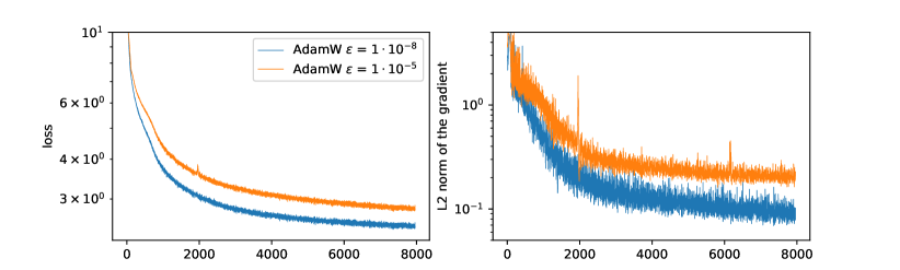
Figure 9: Setting AdamW’s $\epsilon$ to $10^{-8}$ lowers and stabilizes the norm of the gradient early in training. The training loss also improves faster. This trend continues even with runs that are longer than what is shown here.

3.4.2 Weight decay on embeddings

Figure 10 shows the change in training dynamics following a decision to exclude weight decay for embeddings. OLMo uses a standard formulation of weight decay, where every parameter is multiplied by $1-(0.1\cdot lr)$ at every step. This regularization term discourages parameters from growing too large, but in the case of token embeddings it overshoots the mark and results in very small embeddings. As discussed by Takase et al. (2024), small embeddings can produce large gradients in early layers because the Jacobian of $\mathsf{layer\_norm}(x)$ w.r.t. $x$ is inversely proportional to $\left\lVert x\right\rVert$, and, in early layers, the norm of the residual stream is essentially the norm of the embeddings. We experiment with the full range of remedies discussed in Takase et al. (2024), but found that they impacted the speed of convergence. Instead, we simply turn off weight decay for embeddings and observe that embedding norms settle in a healthy region as training progresses.

Figure 10: Weight decay applied to token embeddings leads to a gradual decrease in the embedding norm and a corresponding increase in the gradient norm. Decaying embeddings also has a modest negative impact on stability, producing more spikes than a comparable run without (spike scores of 0.16 and 0.092 respectively).

3.5 Studying the impact of learning rate

Our starting point for learning rate experiments was the setting from Grattafiori et al. (2024). To initialize the optimizer state for the 7B variant, we linearly warm up the learning rate to its peak of $3\cdot 10^{-4}$ over the first 2000 steps. Then, we use a standard cosine decay over 5T tokens. Previous experience with OLMo-0424 suggests that the last part of a cosine decay schedule can be cut off and replaced by a linear decay to zero with little loss of performance. Accordingly, for the 7B variant, we stop the schedule at 4T tokens and then switch to mid-training as described in Section §4. The 13B ran with a higher peak learning rate from the start, so we decided to run it to 5T tokens before moving to the mid-training stage.

Figure 11 shows different runs with four additional learning rate values: $6\cdot 10^{-4}$, $9\cdot 10^{-4}$, $12\cdot 10^{-4}$, and $30\cdot 10^{-4}$. In particular, we tried double, triple, quadruple, 10$\times$, and 30$\times$ the original learning rate. The last, $30\cdot 10^{-4}$, showed training instabilities already during learning rate warm-up, with several loss spikes that did not recover fully, so we abandoned this variant quickly. The other values trained normally and showed an interesting pattern. Looking purely at training loss, higher learning rates universally perform better early on (as long as they avoid loss spikes), but eventually the lower learning rate setting overtakes the others (Figure 11). Notably, when comparing $3\cdot 10^{-4}$ and $6\cdot 10^{-4}$, the cross-over point is well past 200B tokens. A shorter hyperparameter experiment might come to the wrong conclusion.

Figure 11: Higher learning rates perform better at first but are eventually overtaken by lower rates. However, linearly decaying the learning rate to zero over 50B or 100B tokens results in equivalent training loss.

One of the motivations for this line of experimentation was to find out whether a higher learning rate would make the annealing step more effective. The conjecture is that the worse training loss during pretraining is compensated for when the learning rate decays to zero. To test this hypothesis, we took a checkpoint from each of our four variants after 300B tokens, and decayed the learning rate to zero over 50B tokens. To account for the possibility that the effect of higher learning rates needs more steps to unfold, we tried the three higher settings and decayed the learning rate over 100B tokens, for a total of seven experiments. The results show that a higher learning rate does make mid-training more effective, but it does so by exactly the amount that the pretraining is worse. All four variants show the same training loss at the end of the procedure, though the lowest setting lags behind the others by a small amount.

Table 8 shows that the result is consistent for longer training runs as well. We took two variants, $3\cdot 10^{-4}$ and $6\cdot 10^{-4}$, and repeated the experiment after training for 1T and for 2T tokens. We chose these variants because $3\cdot 10^{-4}$ is the baseline from Grattafiori et al. (2024), and $6\cdot 10^{-4}$ showed, by a slim margin, the best training loss. Our results show virtually no difference between the two settings, both on training loss and a mix of nine downstream tasks from the OLMES suite (Gu et al., 2024) shown in Table 8. Evaluating the models on downstream tasks is noisier, but mirrors the findings based on training loss only.

Learning Rate	Pretraining Stage	Mid-training Stage	OLMES (CF, valid)
$3\cdot 10^{-4}$	300B tokens	50B tokens	62.5
$6\cdot 10^{-4}$	300B tokens	50B tokens	63.9
$9\cdot 10^{-4}$	300B tokens	50B tokens	64.1
$12\cdot 10^{-4}$	300B tokens	50B tokens	63.6
$6\cdot 10^{-4}$	300B tokens	100B tokens	64.6
$9\cdot 10^{-4}$	300B tokens	100B tokens	64.5
$12\cdot 10^{-4}$	300B tokens	100B tokens	64.2
$3\cdot 10^{-4}$	2T tokens	100B high quality tokens	73.8
$6\cdot 10^{-4}$	2T tokens	100B high quality tokens	73.9

Table 8: Results on 9 multiple-choice tasks from the validation subset of OLMES (cloze formulation format) for various peak learning rates and schedule lengths. Average scores vary by less than two points across all variants, with most scores within half a point of each other.

Finally, we wanted to see if a higher learning rate during the pretraining stage would result in a more effective mid-training stage when switching to higher quality data. To match our training setup as much as possible within the available compute budget, we took the same two settings ($3\cdot 10^{-4}$ and $6\cdot 10^{-4}$), and linearly decayed the learning rate to 0 over 100B high quality tokens. Once again, the results show little difference. The final scores on the OLMES evaluation suite are within 0.1 points of each other. However, looking at other metrics may still reveal a meaningful difference between the two settings. The mix of high quality tokens targets math specifically, and on GSM8K (which is not part of the OLMES suite), the high learning rate setting is 2.8 points better than the lower learning rate. More study is needed to turn this interesting data point into a dependable result.

This finding contradicts machine learning folk wisdoms such as “higher learning rates are always better” or “area under the learning curve matters” (McCandlish et al., 2018). It expands on Wortsman et al. (2023), who observed that smaller models’ performance is largely invariant to learning rate over several orders of magnitude when trained to the end of a cosine schedule, and further found that QK-norm (section 3.3.2) and z-loss (section 3.3.3), which we use as well, enhance this effect. We find that these results still hold even at much larger scales of tokens and parameters, and, crucially for our training efforts, with our modified learning rate schedule.

Due to cost concerns we did not explore the full range of learning rates. This is the main limitation of this line of experimentation. It would be interesting to run a wider sweep of learning rates to accurately define the boundaries of the plateau we appear to be training in.

4 Deep Dive: Mid-training Recipe

Recent works have suggested that a multi-stage approach to base model training can lead to measurable improvements in capabilities (Blakeney et al., 2024; Ibrahim et al., 2024; Feng et al., 2024). In previous OLMo iterations, we also found that both learning rate schedule (OLMo 1; Groeneveld et al. 2024) and data mixture (OLMo-0424; Ai2 2024) play an important role. We refer to interventions at this stage of model development as mid-training.

For OLMo 2, we significantly refined our mid-training strategy. From afar, our approach is simple: after the pretraining stage, we generate domain-specific data mixtures and re-start training, linearly driving the learning rate down to zero. Our goal is to imbue specialized knowledge and improve capabilities; feedback on these improvements comes from key benchmarks, such as math-specific tasks such as GSM8K.

We collectively refer to the dataset and mixtures created for this mid-training stage as Dolmino Mix 1124. An overview of the contents of this dataset is provided in Section §2.1 (Table 2). In detail, we use the following procedure in our mid-training recipe:

• Identify a mix of high-quality sources to improve performance across the entire development benchmark suite (Section §4.1).

• For patching specific capabilities (specifically, in the case of OLMo 2, math), collect and evaluate domain-specific datasets to mix during mid-training (Section §4.2). We found that these sources can be independently assessesed through a technique we dub microannealing (Section §4.2.2); their effectiveness persists when mixed with rest of sources.

• Following experiments described in Section §3.5, we mix high-quality sources and math-specific data in three different token budgets (50B, 100B, 300B). The smaller mix is used to mid-train OLMo 2 7B, while OLMo 2 13B is annealed on the larger ones. For both OLMo 2 7B and 13B, we find that averaging weights of different checkpoints trained on same mixture but different data order seeds consistently improves over individual checkpoints (Section §4.3).

		Dev Benchmarks						Held-out Evals
Checkpoint	Avg	MMLU	$\textbf{\leavevmode\nobreak\ ARC}_{\textbf{\leavevmode\nobreak\ C}}$	HSwag	WinoG	NQ	DROP	AGIEval	GSM8K	$\textbf{\leavevmode\nobreak\ MMLU}_{\textbf{\leavevmode\nobreak\ PRO}}$
OLMo 2 7B
Pretraining	50.6	59.8	72.6	81.3	75.8	29.0	40.7	44.6	24.1	27.4
Pretraining & mid-training	61.2	63.7	79.8	83.8	77.2	36.9	60.8	50.4	67.5	31.0
OLMo 2 13B
Pretraining	56.5	63.4	80.2	84.8	79.4	34.6	49.6	48.2	37.3	31.2
Pretraining & mid-training	66.8	67.5	83.5	86.4	81.5	46.7	70.7	54.2	75.1	35.1

Table 9: Evaluations comparing OLMo 2 7B and 13B at the end of pretraining and mid-training stages (setup mirrors Table 6). Pretrain checkpoints have been trained on 4 trillion (7B) and 5 trillion (13B) tokens respectively. For 7B, we obtain the final mid-train checkpoints by averaging three training runs on 50B Dolmino tokens; for 13B, we use three runs on 100B tokens and one run on 300B tokens.

Table 9 summarizes the dramatic impact of this mid-training phase on both development and held-out evals. OLMo 2 7B model improves, on average by 10.6 points, surpassing the larger 13B model after the pretraining stage. For its part, OLMo 2 13B benefits equally from mid-training, improving its average performance by 10.3 points. Both models see improvements in knowledge-intensive, multiple-choice (Arc challenge: $72.6\rightarrow 79.8$ for 7B, $80.2\rightarrow 83.5$ for 13B; MMLU: $59.8\rightarrow 63.7$ for 7B, $63.4\rightarrow 67.5$ for 13B; AGIEval: $44.6\rightarrow 50.4$ for 7B, $48.2\rightarrow 54.2$ for 13B), reading comprehension (Natural Questions: $29.0\rightarrow 36.9$ for 7B, $34.6\rightarrow 46.7$ for 13B; DROP: $40.7\rightarrow 60.8$ for 7B, $49.6\rightarrow 70.7$ for 13B), and math skills (GSM8K: $24.1\rightarrow 67.5$ for 7B, $37.3\rightarrow 75.1$ for 13B) benchmarks.

4.1 Dolmino Mix 1124: High Quality Sources

	Source		Mix %
			PT Mix	Web ${}^{\text{{\sans{FT}}}_{\text{{\sans{7}}}}}$	Web ${}^{\text{{\sans{FT}}}_{\text{{\sans{7}}}}}_{\text{{\sans{FW}}}_{\text{{\sans{3}}}}}$	Web ${}^{\text{{\sans{FT}}}_{\text{{\sans{7}}}}}_{\text{{\sans{FW}}}_{\text{{\sans{2}}}}}$	Web ${}^{\text{{\sans{FT}}}_{\text{{\sans{7}}}}}_{\text{{\sans{FW}}}_{\text{{\sans{2}}}}}$ + Math	Web ${}^{\text{{\sans{FT}}}_{\text{{\sans{7}}}}}_{\text{{\sans{FW}}}_{\text{{\sans{2}}}}}$ + Ins	Web ${}^{\text{{\sans{FT}}}_{\text{{\sans{7}}}}}_{\text{{\sans{FW}}}_{\text{{\sans{2}}}}}$ + Math + Ins
	DCLM	from pretrain	95.2	-	-	-	-	-	-
	DCLM	FT top 7%	-	57.1	-	-	-	-	-
	DCLM	FT top 7% $\text{FineWeb}\geqslant 3$	-	-	54.2	-	-	-	-
WEB	DCLM	FT top 7% $\text{FineWeb}\geqslant 2$	-	-	-	57.9	61.8	75.5	57.5
	Flan	Dolma 1.7 decontaminated	-	-	-	-	-	8.8	6.7
INST	Stack Exchange	2024/09/30 dump Q&A format	-	-	-	-	-	0.7	0.5
	Starcoder	from pretrain	2.1	19.5	20.9	19.2	-	-	-
CODE	CodeSearchNet	unfiltered	-	-	-	-	0.1	0.2	0.1
	Gutenberg Books	from Dolma 1.7	-	1.2	1.3	1.2	-	-	-
	peS2o	from pretrain	1.5	6.6	7.1	6.5	10.7	13.0	9.9
	Wikipedia	from pretrain	0.1	0.9	0.9	0.9	1.6	1.9	1.4
	StackExchange	from RedPajama v1	-	4.0	4.3	4.0	-	-	-
REFERENCE	ArXiv	from pretrain	0.5	4.9	5.2	4.8	-	-	-
	Algebraic Stack	from pretrain	0.3	2.8	3.0	2.7	-	-	-
	OpenWebMath	from pretrain	0.3	2.9	3.1	2.8	5.2	-	4.8
	GSM8k	train split	-	-	0.003	0.003	0.003	-	0.003
	Mathpile	commercial subset train split	-	-	-	-	2.1	-	1.9
MATH	AutoMathText	unfiltered	-	-	-	-	18.5	-	17.2

Table 10: A summary of high-quality sources we evaluate for mid-training. We experiment with mixing these sources in 6 mixes, each consisting of 50 billion tokens. Percentages on the table indicate the fraction of each 50B mix that is comprised by data from the respective source. PT Mix is sampled (with repetition) from the pretraining stage.

Following the recipe from the previous OLMo iteration (Ai2, 2024), we start by curating a higher quality subset of pretraining mix, and expand it with more academic and encyclopedic material. In particular, we consider the following sources (summarized in Table 10):

High quality web

To filter the web subset used in pretraining, we experiment with two existing quality classifiers:

• FastText classifier from Li et al. (2024). To train this model, Li et al. sampled positive documents from the Reddit subset in ELI5 (Fan et al., 2019), and demonstrations from Open Hermes 2.5. Negatives are sampled at random from the DCLM pipeline.

• FineWeb Edu classifier from Penedo et al. (2024). This model is fine-tuned from the Arctic Embed M encoder (Merrick et al., 2024) on over 400,000 web pages labeled by Llama 3 70B Instruct. This classifier scores documents from 0 to 5 according to adherence to academic topics and polished content.

Following Li et al. (2024), we use the DCLM FastText classifier with a threshold of $0.03311014$, which retains approximately 65.6% of the web subset. We combine this filter with the the scores from FineWeb Edu classifier; we experiment by retaining documents with score over 3 (5.8% retained), as well as a more relaxed threshold of 2 (20.3% retained).

Instruction data and Q&A pairs

We leverage the same subset of FLAN Wei et al. (2021); Longpre et al. (2023) from Dolma 1.7 (Soldaini et al., 2024). We decontaminated this source by extracting training, validation, and test instances from all tasks in our evaluation suite (Section §2.4) and removed FLAN documents with 10% or more overlapping ngrams with any task instance.

We source question and answer pairs from the Stack Exchange network, a collection of 186 forums dedicated to a wide variety of topics. Content on Stack Exchange network is licensed under various commercial-friendly Creative Common licenses. We use the latest database dump (September $\text{30}^{\text{th}}$, 2024) at the time of writing, which is distributed by the Internet Archive. We filter questions to those that have an accepted answer; further, we Q&A pairs whose questions have fewer than 3 votes or answers have fewer than 5 votes. Once filtered, we concatenate questions and answers together using a sequence of new lines that contains one more \n than longest sequence of newlines in either the question or answer.

Code

We evaluate retaining the same subset of code used during pretraining; furthermore, we consider smaller, curated sources of code interleaved with natural supervision, such as docstrings in CodeSearchNet (Husain et al., 2019); Q&A pairs from StackExchange described in the paragraph above also contain code.

Academic, encyclopedic and other reference content

We source high-quality non-web datasets from Dolma 1.7 (Soldaini et al., 2024). This includes peS2o (Soldaini and Lo, 2023), Wikipedia, and Wikibooks, Gutenberg books, arXiv and StackExchange (from Red-Pajama v1; Together AI, 2023), Algebraic Stack (ProofPile II; Azerbayev et al., 2023).

Math

In parallel to developing the math subset of Dolmino Mix 1124 (Section §4.2), we consider preliminary math subset to gauge how math documents combine with the non-math portion of the mix. In particular, we used OpenWebMath (Paster et al., 2023), the train split of GSM8K (Cobbe et al., 2021), the train split of the permissively licensed (“commercial”) subset of MathPile (Wang et al., 2023b), and AutoMathText (Zhang et al., 2024b).

Mid-training mix	OLMES (MCF)	OLMES-Gen	MMLU (MCF)	GSM*
n/a (pretrain checkpoint)	69.6	63.2	59.8	28.5
PT Mix	74.0	64.5	61.8	27.0
Web ${}^{\text{{\sans{FT}}}_{\text{{\sans{7}}}}}$	73.5	64.1	61.9	24.5
Web ${}^{\text{{\sans{FT}}}_{\text{{\sans{7}}}}}_{\text{{\sans{FW}}}_{\text{{\sans{3}}}}}$	73.5	63.0	62.4	30.5
Web ${}^{\text{{\sans{FT}}}_{\text{{\sans{7}}}}}_{\text{{\sans{FW}}}_{\text{{\sans{2}}}}}$	75.2	63.8	63.1	28.5
Web ${}^{\text{{\sans{FT}}}_{\text{{\sans{7}}}}}_{\text{{\sans{FW}}}_{\text{{\sans{2}}}}}$+ Ins	74.2	64.1	63.0	46.0
Web ${}^{\text{{\sans{FT}}}_{\text{{\sans{7}}}}}_{\text{{\sans{FW}}}_{\text{{\sans{2}}}}}$+ Math	75.7	69.7	62.3	52.0
Web ${}^{\text{{\sans{FT}}}_{\text{{\sans{7}}}}}_{\text{{\sans{FW}}}_{\text{{\sans{2}}}}}$+ Math + Ins	75.7	70.2	63.1	46.5

Table 11: Comparison of mid-training mixes introduced in Table 10. Each row corresponds to a 50 billion token training run following learning rate schedule described in Section §3.5 (except first row). Weights are initialized from a OLMo 2 checkpoint pretrained for 4T tokens. We compare each run on a mix of OLMES core tasks (multiple choice format; see Table 28), OLMES generative tasks (Table 22), MMLU (multiple choice format; Hendrycks et al., 2021), and a random sample of 200 GSM8K (Cobbe et al., 2021) questions we use as development set (GSM*; Section §A). Results on the final mid-training mix are in Table 9.

Results of mixes shown in Table 10 are summarized in Table 11. All results correspond to mid-training runs on 50 billion tokens, initialized from a 7B model checkpoint pretrained on 4 trillion tokens.

We find that, as noted in Section §3.5, learning rate anneal (PT Mix) alone yields notable improvements across all averages (OLMES $+4.4$; OLMES-Gen $+1.3$; MMLU $+20$), but not on our math development set (GSM* $-1.5$). Switching to mixes that contain higher quality web data and reference content further improves performance: Web ${}^{\text{{\sans{FT}}}_{\text{{\sans{7}}}}}_{\text{{\sans{FW}}}_{\text{{\sans{2}}}}}$ further improves $+1.2$ points over PT Mix in OLMES and $+1.3$ in MMLU; it is slightly worse on OLMES-Gen ($-0.4$) and within margin of error on GSM* ($+1.5$). Finally including instruction data and math source in the mix yields the best performance. Web ${}^{\text{{\sans{FT}}}_{\text{{\sans{7}}}}}_{\text{{\sans{FW}}}_{\text{{\sans{2}}}}}$+ Math + Ins mix achieves best overall results, with $+1.7$ on OLMES, $+5.7$ on generative tasks, $+1.3$ on MMLU, and $+19.5$ on GSM*. We note that Web ${}^{\text{{\sans{FT}}}_{\text{{\sans{7}}}}}_{\text{{\sans{FW}}}_{\text{{\sans{2}}}}}$+ Math mix performs slightly better on math tasks, motivating our investigation in better math subsets that combine well with other high-quality sources in Section §4.2.

4.2 Dolmino Mix 1124: Math Mix

Early mid-training mixes ($\text{\sans{Web}}_{\ast}^{\ast}$ only rows in Table 11) show models struggle in math-related benchmarks. Thus, improving performance on these sets is a central focus of our mid-training investigations. We investigate both human-authored and synthetically generated or augmented data; we derived the latter through an iterative procedure aimed at fixing common errors in our math validation sets.

We describe both the data sources and their generation/filtration procedure in Section §4.2.1; then, in Section §4.2.2, we detail microanneals, the experimentation technique we use to finalize math sources. The resulting mix is summarized in Table 2.

4.2.1 Math Sources

TuluMath

We follow the recent persona-driven methodology in Chan et al. (2024) to generate math synthetic data. The key idea is to use different personas (e.g., “A machine learning researcher focused on neural networks”) with a data synthesis prompt (e.g., “create a math problem”) to steer an LM to synthesize data with corresponding perspectives. Specifically, we condition on available personas from Persona Hub (Chan et al., 2024) to generate prompts targeting Math problems both those that require advanced mathematical skills as well as grade school problems. We zero-shot-prompt GPT-4o to generate problems that are unique and specific to a given persona input. Having generated the problems, we then generate multi-step math solutions using GPT-4o. Exact prompts used to generate problems and solutions are provided in Appendix Figures 23 and 24. In total, we collected $\sim$ 230M synthetic math tokens.

DolminoSynthMath

This is a collection of 28M synthetic math tokens designed specifically to improve performance on GSM8K as well as raw mathematical calculations. It is composed of three parts: first we generate 11M tokens of basic mathematical question and answer pairs such as “77 * 14 = 1078” and pair each of these with a variety of prompts. We find that including such data dramatically mitigates the mistakes our model makes within individual CoT reasoning steps at inference time. Next we include a custom collection of 7,924 synthetic GSM8K examples, which are produced by consuming a GSM8K training example and replacing all of its numbers in both the provided question and answer, with the hope that this would provide signal to the model to extract the computation graph from a word problem and ignore irrelevant semantic features. Finally we include a MIND-rewriting (Akter et al., 2024) of each of the GSM8K training examples, where the synthetic data was generated using Qwen2.5-7B-Instruct (Qwen et al., 2024).

TinyGSM-MIND

We generated approximately 6.5B tokens of synthetic math data from rewritten versions of Tiny-GSM (Liu et al., 2023a). Tiny-GSM is a collection of 11M synthetic GSM8K-like questions, where the answers are provided in the form of python code. We filter this set to only include answers that have code that is executable and only contains statements that are variable assignments. We then annotate each line of the code that is an assignment operator with the numerical value of the resulting variable. Then we pass all of these annotated examples to Qwen2.5-7B-Instruct to be rewritten in the style of MIND (Akter et al., 2024) using the ‘Two Students’ and ‘Problem Solving’ prompts.

MathCoder2-Synthetic

We emulate the synthetic data generation procedure of MathCoder2 (Lu et al., 2024) to filter existing synthetic data from open-source repositories. In particular, we collect the synthetic textbooks from HuggingFace user Ajibawa-2023,${}^{\text{,}}$ and from the M-A-P Matrix dataset and perform additional filtering on them. In particular we train a FastText classifier as follows: we ask GPT-4o to annotate 10,000 OpenWebMath examples (Paster et al., 2023) as either math-related or non-math-related; we then use these as positive and negative examples for a FastText classifiers. We apply this classifier to the synthetic textbooks and only keep the math-related ones.

ProofPile OWM-Filtered

We use the same OpenWebMath filter generated in the previous step and apply it to Metamath (Yu et al., 2023) and CodeSearchNet (Husain et al., 2019).

GSM8K-Train

Finally, we include the training split of GSM8K (Cobbe et al., 2021).

4.2.2 Evaluating Math Data with Microanneals

To select the highest quality subset of all available and synthetic math data, we perform a series of several microanneals, which were annealing runs focused on small math subsets. The general recipe for these microanneals is as follows:

1. identify a source or small collection of math sources that we want to assess the data quality of;

2. collect roughly the same quantity of data from the general data mix (e.g., DCLM) as from the math sources to ensure a mixtureof high-quality web text alongside domain-specific math;

3. train this 50/50 mixture as if it were an annealing run, making sure to linearly drive the learning rate down at the proper rate for this smaller collection of data.

This procedure facilitates evaluating the quality of individual data sources at a fraction of the cost of a full annealing run. In total, we run 19 separate microanneals with a total token count of 130B tokens, equivalent to less than 3 full 50B annealing runs. Putting this cost into perspective, the totality of the 19 microanneals requires less compute than the 3 50B token souping ingredients used for our 7B model. More explicitly, it shows improvements at a much finer-grained data-source resolution, with results visible after training for less than 10B tokens.

Microanneal Experiment 1
Mix	Web ratio	Tokens	MMLU (avg)	GSM*
Baseline	n/a	n/a	59.8	28.5
Math 35/65	65.0%	576M	60.1	63.5
Math 10/90	88.3%	1.72B	60.9	61.0
Microanneal Experiment 2
Mix	Web ratio	Tokens	MMLU (avg)	GSM*
Baseline	n/a	n/a	59.8	28.5
1x Math	65.0%	576M	60.1	63.5
2x Math	49.3%	798M	60.3	66.0
4x Math	48.6%	1.57B	60.5	65.0
Microanneal Experiment 3
Mix	Web ratio	Tokens	MMLU (avg)	GSM*
Baseline	n/a	n/a	59.8	28.5
TinyGSM-Inline	47.9%	3.17B	60.4	25.0
TinyGSM-MIND	52.1%	6.40B	61.4	65.5
2x TinyGSM-MIND	51.3%	12.6B	62.1	70.0

Table 12: Results from microanneal experiments to OLMo 2 math capabilities. We evaluate math/not-math mixture ratio, impact of repeating math tokens, and different math datasets. We use a random sample of 200 GSM8K (Cobbe et al., 2021) questions we use as development set (GSM*; Section §A) as a proxy for math capabilities. We monitor average MMLU scores to ensure OLMo 2 remains performant on knowledge intensive tasks.

We illustrate how microanneals lead to our final math mix through three sets of experiments reported Table 12. The primary evaluation metrics we use to evaluate the quality here is MMLU, and GSM*, which is our 200-example subset of the GSM8K evaluation set. Note that one goal of mid-training is to improve GSM8K performance, but we only allow ourselves to inspect performance on 200 of the 1319 GSM8K examples to inform decisions about data mixtures.

Microanneal experiment 1: domain specific data is helpful even in small proportions

We run the following experiment: starting from a 7B model that has completed pretraining, and a mixture of TuluMath, DolminoSynthMath, Metamath, CodeSearchNet, and GSM8K-Train, accounting for approximately 200M tokens, we train on both a 35/65 math/DCLM mixture and a 10/90 mixture and evaluate both the MMLU and GSM*. We see that the pre-anneal had a GSM* score of 28.5, the 35/65 mixture yields a GSM* of 63.5, and the 10/90 mixture yields a GSM* of 61. This suggests that it is not strictly necessary to have a large proportion of domain-specific data in the annealing mixture, just that domain-specific data is present.

Microanneal experiment 2: some duplication is beneficial

Starting from the same setup as the previous experiment, we duplicate the math data for a total of two copies, and four copies. We see that one copy of the math yields a GSM* score of 61, two copies yields a score of 66, and four copies yields a score of 65. This suggests that even if there is a scarcity of high-quality domain-specific data, duplicating it a small number of times can still provide some gains.

Microanneal experiment 3: rewriting can help dramatically

Here we once again start with a 7B model that has completed pretraining and evaluate the effect that rewriting Tiny-GSM into a natural language format has on GSM* evaluation scores. Recall that Tiny-GSM has answers written in the form of code, and that our pretraining mix is only 2% code. We run a microannealing run on a mixture using an inline-annotated form of TinyGSM and compare it to just the ‘Problem Solving’ MIND rewritten variant of TinyGSM. Relative to the baseline, the code version of TinyGSM degrades GSM* performance, while the rewritten version dramatically improves the performance. This suggests the power of rewriting as a tool to cheaply convert data to a more amenable form for training.

4.3 Final Midtraining mix and Checkpoint Soups

Source Tokens 50B 100B 300B Source % Mix % Source % Mix % Source % Mix % Filtered DCLM 752B 3.23 47.2 6.85 50.2 20.78 51.9 Decontam. FLAN 17.0B 50.0 16.6 100 16.7 200 11.3 StackExchange Q&A 1.26B 100 2.45 200 2.47 400 1.68 peS2o 58.6B 5.15 5.85 16.7 9.52 100 19.4 Wikipedia/Wikibooks 3.7B 100 7.11 100 3.57 400 4.86 Dolmino Math 10.7B 100 20.8 200 17.5 400 10.8

Table 13: Dolmino Mix 1124 compositions. The Source % column indicates the fraction of the source that was used in the Dolmino mix. Numbers in this column greater than 100 indicate we used the data, e.g. 400 indicates a 4x repeat. The Mix % column describes the proportion of the Dolmino mix that is composed of this source, i.e., this column should sum to 100%.

The final composition of Dolmino Mix 1124 is shown in Table 2. As previously mentioned, we sample 3 mixes of 50B, 100B, and 300B tokens; composition of each is summarized in Table 13. Since experiments in Section §4.1 and §4.2.2 show that keeping mixing proportion roughly constant across sources is beneficial, we repeat Stack Exchange Q&A data and mid-training math data twice for the 100B tokens mix, and four times for the 300B mix; additionally, we repeat FLAN twice and Wiki data four times for the 300B mix. Across all mixes, filtered web data from the DCLM baseline represents roughly 50% of the total tokens budget.

We train OLMo 2 7B on the 50B mix. To account for the larger batch size (Section §2.3), we use the 100B mix for OLMo 2 13B, ensuring the same number of steps during learning rate anneal. Further, we experiment with a longer anneal phase with OLMo 2 13B using the 300B mix.

Mid-training mix		OLMES (MCF)	OLMES-Gen	MMLU (MCF)	GSM*
	best single	75.6	68.5	61.2	71.0
A	3 x soup	77.0	69.4	62.0	74.0
	best single	75.3	69.9	61.5	73.0
B	3 x soup	77.3	70.1	62.7	77.0
	best single	76.3	70.9	62.8	66.0
C	3 x soup	76.8	71.3	63.5	66.0
	best single	77.5	71.2	63.4	59.5
D	3 x soup	77.8	71.7	63.5	60.0
	best single	73.4	63.1	62.2	60.5
E	3 x soup	75.3	64.2	63.1	43.0
	best single	77.1	69.9	63.7	73.5
F	3 x soup	77.9	70.4	63.7	74.5

Table 14: Comparison of six mid-training mixes between best single checkpoint and the average of three checkpoints (soup) trained on different data permutations. We run all experiments starting from 7B pretrained checkpoint; we run mid-training stage for 50B tokens. Souping consistently equals or outperform the single best checkpoint trained on the same mix.

Mid-training soups

Performing a naïve average of multiple model checkpoints trained with a different data order has been proven effective in both computer vision (Wortsman et al., 2022) and language modeling (Li et al., 2024) applications. We confirm the effectiveness of this approach, also known as model souping, on six different mid-training mixes, as shown in Table 14. For all experiments, we find that souping 3 checkpoints annealed on three permutations of the same data mix consistently produces equal or better performance than any individual training run.

Based on this evidence, we extensively use model souping to obtain our final OLMo 2 7B and 13B models. For OLMo 2 7B, we average three checkpoints trained on the 50B sample of Dolmino Mix 1124. For OLMo 2 13B, we soup four checkpoints: three trained on the 100B sample, and one trained on a 300B sample; we find this approach to be empirically better than averaging just the three 100B runs alone.

5 Deep Dive: Post-training Pipeline

To adapt OLMo 2 to downstream generative tasks, we follow the Tülu 3 recipe (Lambert et al., 2024) with an increased focus on permissive licenses and suitable adjustments to hyperparameters. The Tülu 3 approach involves three phases of training: supervised finetuning (SFT), preference tuning with Direct Preference Optimization (DPO; Rafailov et al., 2024) and on-policy preference data, and finally Reinforcement Learning with Verifiable Rewards (RLVR). We find that all of the stages in the Tülu 3 Recipe easily translate to the OLMo 2 models.

Category Benchmark CoT # Shots Chat Multiturn ICL Metric Knowledge Recall MMLU ✓ 0 ✓ ✗ EM PopQA ✗ 15 ✓ ✓ EM TruthfulQA ✗ 6 ✓ ✗ MC2 Reasoning BigBenchHard ✓ 3 ✓ ✓ EM DROP ✗ 3 ✗ N/A F1 Math GSM8K ✓ 8 ✓ ✓ EM MATH ✓ 4 ✓ ✓ Flex EM Instruction Following IFEval ✗ 0 ✓ N/A Pass@1 (prompt; loose) AlpacaEval 2 ✗ 0 ✓ N/A LC Winrate Safety Tülu 3 Safety ✗ 0 ✓ N/A Average^∗

Table 15: The OLMo 2 Instruct Evaluation Regime (Adapted from Lambert et al. (2024)): settings for development (top) and unseen (bottom) portions of the evaluation suite. CoT are evaluations run with chain of thought prompting (Wei et al., 2022). # shots is the number of in-context examples in the evaluation template. Chat indicates whether we use a chat template while prompting the model. Multiturn ICL indicates that we present each in-context example as a separate turn in a conversation (applicable only when a chat template is used and # Shots is not 0). ^∗Average over multiple sub-evaluations—full details of the safety evaluation are in Lambert et al. (2024).

Supervised Finetuning (SFT)

The SFT training of OLMo 2-Instruct from Tülu 3 relies on selecting the highest-quality, existing instruction datasets and complementing them with scaled synthetic data for Supervised Finetuning based on the PersonaHub method (Chan et al., 2024). The final SFT mix used for OLMo has 939,104 prompts.

Given that OLMo 2 is not trained for multilingual tasks, we experimented with removing all multilingual data from the SFT stage. When removing the entire Aya split and the multilingual samples of Wildchat from Tülu 3, we saw a degradation of $\sim 0.5$ points on average, indicating that the Tülu 3 dataset is balanced and cannot be easily improved by removing irrelevant subsets.

	AVG	AE2	BBH	DROP	GSM8K	IFE	MATH	MMLU	Safety	PQA	TQA
OLMo 2 7B SFT	50.2	10.2	49.6	59.6	74.6	66.9	25.3	61.1	82.1	23.6	48.6
OLMo 2 7B DPO	54.6	27.9	51.1	60.2	82.6	73.0	30.3	60.8	81.0	23.5	56.0
OLMo 2 7B Instruct	55.2	29.1	51.4	60.5	85.1	72.3	32.5	61.3	80.6	23.2	56.5
OLMo 2 13B SFT	55.4	11.5	59.9	71.3	76.3	68.6	29.5	68.0	82.3	29.4	57.1
OLMo 2 13B DPO	60.9	38.3	61.4	71.5	82.3	80.2	35.2	67.9	79.7	29.0	63.9
OLMo 2 13B Instruct	62.4	39.5	63.0	71.5	87.4	82.6	39.2	68.5	79.1	28.8	64.3

Table 16: Comparison of performance for OLMo 2 Instruct after different training stages. The final Instruct model is from the RLVR stage. The following evaluation names are abbreviated: AVG – Average, AE2 – AlpacaEval 2, BBH – BigBenchHard, IFE – IFEval, PQA – PopQA, TQA – TruthfulQA.

Epochs	L.R.	Loss	Avg. Perf.
2	1e-5	sum	49.97
3	4e-6	sum	49.76
2	1e-5	sum	49.74
2	1e-5	sum	49.59
3	4e-6	mean	48.25
2	2e-6	mean	48.18

Table 17: Hyperparameter configurations tried for the 7B SFT checkpoint, all on the same dataset used in the final model.

Figure 12: The average score for DPO checkpoints trained on a development SFT checkpoint on different learning rates. Avg does not include Safety.

Preference Finetuning (PreFT) with DPO

The core strategy of the Tülu 3 pipeline for PreFT is building upon and scaling the UltraFeedback pipeline (Cui et al., 2023) for generating synthetic preferences across data for our target domains. We include on-policy data by sampling responses from some development OLMo 2 SFT models at both 7B and 13B, with independent datasets for each.

From Tülu 3, we updated our model pool to only include models with permissible licenses as shown in Table 25 in the Appendix. We made a minor shift from Tülu 3 on the exact prompts used for DPO – we obtain our prompts from several sources listed in Table 27, resulting in datasets of 366.7k prompts for 7B and 377.7k prompts for 13B. Given this set of prompts, we generate responses from a pool of 20 models of different families and sizes.

To create synthetic preference data we use GPT-4o-2024-08-06 as an LM judge (Zheng et al., 2023) and prompted it to rate completions based on helpfulness, truthfulness, honesty, and instruction-following aspects. We then binarize the ratings across aspects by following Argilla’s method: we get the average rating across all aspects, take the highest-rated completion as the chosen response, and sample from the remaining completions for the rejected response.

Reinforcement Learning with Verifiable Rewards (RLVR)

RLVR is a novel finetuning technique used to target specific domains where prompts with verifiable answers can be constructed. For example, with a math problem, the RL algorithm Proximal Policy Optimization (PPO) (Schulman et al., 2017) only receives a reward if the answer is correct. For more details, see Lambert et al. (2024).

Following preference tuning, we trained 7B and 13B reward models using the on-policy 7B and 13B preference dataset. Next, we applied RLVR to the highest-performing 7B and 13B DPO checkpoints with a combined dataset comprising GSM8K, MATH training sets, and prompts with constraints from Lambert et al. (2024). For RLVR, we initialize PPO’s value function from the corresponding RMs, which is shown to help improve average scores across evaluations (Lambert et al., 2024). After the initial RLVR training pass on the 13B model, we observe that its performance on GSM8K and MATH was lower than a previous development instruct model. Consequently, we perform two additional RLVR training iterations: first on the GSM8K training set, followed by the MATH training set. The models selected at the end of the RLVR stage constitute the final OLMo 2 Instruct models.

OLMo-2-1124-13B-RLVR1 OLMo-2-1124-13B-RLVR2 OLMo-2-1124-13B-Instruct (Final RLVR)

Figure 13: The scores from our evaluation suites for OLMo-2-1124-13B-Instruct trained with RLVR. We train OLMo-2-1124-13B-RLVR1 on the GSM8K, MATH, and prompts with constraints dataset mix, but noticed the GSM8K score was lower than expected. We proceed with training OLMo-2-1124-13B-RLVR2 on GSM8K and observed higher GSM8K score. Finally, we train OLMo-2-1124-13B-Instruct on just MATH and observe even higher GSM8K and MATH scores. Note that the value function was re-initialized from the reward model in each RLVR run. The full learning curves of each RLVR run can be found in Appendix B.2.

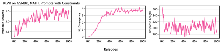
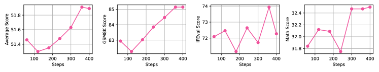
OLMo-2-1124-7B-Instruct

Figure 14: The top row shows the training curves of OLMo-2-1124-13B-Instruct on verifiable rewards, KL divergence, and response lengths. In the bottom row, the y-axes show the average scores across our evaluation suites and GSM8K, IFEval, and MATH Flex scores, respectively. Overall, we find RLVR increases not only the training rewards of our 7B models but also the downstream evaluations such as GSM8K.

Hyperparameter selection

We perform the following hyperparameter tuning:

1. SFT: We sweep over learning rates $1\times 10^{-5}$, $2\times 10^{-5}$, $3\times 10^{-5}$ for the 7B model and $1\times 2^{-6}$, $4\times 2^{-6}$, $5\times 2^{-6}$, $7.5\times 2^{-6}$, $8\times 2^{-6}$ for the 13B model, using 1 or 4 random seeds.

2. DPO: We sweep over learning rates $5\times 10^{-7}$, $6\times 10^{-7}$, $7\times 10^{-7}$, $8\times 10^{-7}$, and $1\cdot 10^{-6}$ for both the 7B model and 13B model, using 1 or 4 random seeds.

3. RM: We train with $3\times 10^{-6}$ learning rate and 1 random seed for the 7B and 13B models, respectively.

4. RLVR: We sweep over beta values 0.03, 0.05, 0.07, and 0.1, using 1 or 4 random seeds. For 13B model, we also sweep over learning rates $3\times 10^{-7}$, $4\times 10^{-7}$, using 1 or 4 random seeds. For 13B, we run this sweep on the best model at each RLVR stage.

We conducted a hyperparameter sweep for SFT and DPO, using earlier development checkpoints, with results detailed in Table 17 and Figure 12. A key finding was that OLMo 2 required significantly higher learning rates compared to the Llama 3.1 training recipe described by Lambert et al. (2024). Finally, the optimized hyperparameters for our final model are presented in Table 17 and Table 18.

Evaluation of OLMo 2-Instruct

Following Tülu 3 (Lambert et al., 2024), we evaluate OLMo 2-Instruct on five categories listed in Table 15. Although Tülu 3 uses six categories including code-related tasks, we exclude this category since code was not a target skill during the development of OLMo 2. For each of the remaining categories, we use the same evaluations as those used for developing the Tülu 3 recipe. Table 15 also shows the settings and metrics used for each of the evaluations. These match those recommended in Lambert et al. (2024) for the non-code categories.

Table 16 presents the performance of OLMo 2 Instruct variants across different training stages. A comparative analysis of OLMo 2-Instruct’s performance against similarly-sized open models can be found in Table 7. Furthermore, Figures 13 and 14 present the training trajectories and key performance metrics for the 13B and 7B models, respectively.

The OLMo 2-Instruct models demonstrate comparable performance to leading open-weight models in the field. Specifically, OLMo 2 13B Instruct achieves results approaching those of Qwen 2.5 14B Instruct while surpassing both Tülu 3 8B and Llama 3.1 8B Instruct in performance benchmarks. The RLVR stage also demonstrated consistent effectiveness across both model scales, leading to notable improvements in evaluation metrics in tandem with increasing the training reward signal.

Finally, we evaluate OLMo 2-Instruct on the unseen evaluation suite from Lambert et al. (2024) without the code evaluation tasks. The Instruct scores on the unseen evaluation suite are shown in Table 24.

Hyperparameter	RLVR value
Learning rate	$3\cdot 10^{-7}$ for 13B; $4\cdot 10^{-7}$ for 7B
Effective batch size	248 for 13B; 224 for 7B
KL penalty coef. ($\beta$)	0.1 for first and final 13B; 0.03 for second 13B; 0.05 for 7B
Max total episodes	200,000 for 13B; 100,000 for 7B
Discount factor $\gamma$	1.0
General advantage estimation $\lambda$	0.95
Mini-batches $N_{\text{mb}}$	1
PPO update iterations $K$	4

Hyperparameter	RLVR value
PPO’s clipping coefficient $\varepsilon$	0.2
Value function coefficient $c_{1}$	0.1
Gradient norm threshold	1.0
Learning rate schedule	linear
Generation temperature	1.0
Max token length	2,048
Max prompt token length	2,048
Penalty reward for no EOS token	$-10.0$
Response length	2,048
Warm up ratio ($\omega$)	0.0

Table 18: The hyperparameters of PPO used for optimizing against the verifiable reward function with RLVR. Hyparameters with different settings for the 7B and 13B parameter models are highlighted.

6 Deep Dive: Infrastructure as a Research Catalyst

LM training is famously compute intensive. Training large models requires state-of-the-art hardware, and a lot of work goes into making it run efficiently. Gains in efficiency can be translated into higher token counts or more parameters, directly affecting the quality of the final model. GPUs are at the core of this infrastructure, investment in other processes and systems is required to make them perform at peak efficiency. Data centers need high-speed interconnect between compute nodes to make sure expensive GPUs never have to wait for data to arrive. Training jobs need access to large amounts of fast, reliable storage for access to training data. GPUs have higher failure rates than most other hardware, and a single training run might require thousands of them at the same time, making effective monitoring and replacement policies a necessity. This section provides details about our hardware and software investments to support OLMo 2 workloads.

6.1 Clusters

OLMo 2 is trained on two Ai2 clusters, Jupiter and Augusta. Despite hardware and architectural differences, both clusters provided sufficient training throughput. Beaker, Ai2’s workload management system, allows researchers to migrate workloads from one cluster to another, and both the 7B and 13B variants were trained partially on both clusters, with the bulk of the 7B training on Jupiter, and the bulk of 13B training on Augusta.

6.1.1 Jupiter

Jupiter is a 128-node GPU cluster located in Austin, Texas. It is operated by Cirrascale Cloud Services.

Compute

It consists of 1,024 NVIDIA H100 GPUs, each with 80GB HBM3 running at 700W. The GPUs are spread across 128 servers with 2x Intel Xeon Platinum 8468 CPUs, 2 TB of DDR5 system memory, and 18 TB of local NVMe storage.

Storage

The servers are connected via a 800 Gbps local network to a WEKA high performance storage cluster. This cluster has 1 PB of NVMe SSD storage with 11 physical servers, and 5 PB of HDD storage spread across 12 hosts. The Jupiter GPU servers have two bonded 25 Gbps Mellanox ethernet cards each, providing a total of 50 Gbps of throughput per host. In benchmarks, we reach 761 Gbps of read/write throughput using 64 client machines.

Interconnect

Cross-node GPU communication is provided via RDMA over InfiniBand and a 2-Tier Rail Optimized (Wang et al., 2023a), balanced, full-bisected network. Each physical server has eight 400 Gbps InfiniBand cards, providing a maximum total throughput per host of 3200 Gbps. This setup allows Ai2 to run dozens of distributed training workloads simultaneously on the same cluster without topological scheduling.

Cooling

The Jupiter servers are racked in Dynamic Density Cabinets. Each cabinet includes 5 servers with dedicated cooling and power. Each cabinet is a closed system, circulating air through an overhead compartment where it is cooled via heat transfer to water. This approach allows the datacenter to achieve a power usage efficiency (PUE) of 1.2. Under heavy utilization, our H100 GPUs reach a peak temperature of 75°C; average GPU temperatures are between 60°C and 65°C.

6.1.2 Augusta Cluster

The Augusta cluster is a 160-node GPU cluster provided by Google Cloud. The physical servers are located in Council Bluffs, Iowa.

Compute

The cluster is made up of A3 Mega virtual machines, each with 8 NVIDIA H100 GPUs.

Storage

Augusta workloads use Google Cloud Storage for speeds up to 1 GB/s per VM. We ensure portability by abstracting storage interactions into common libraries supporting both file- and object-based APIs.

Interconnect

Each GPU has a dedicated Ethernet NIC. Fast cross-node GPU communication is achieved using GPUDirect-TCPXO, gVNIC, and compact node placement. This arrangement takes advantage of Google’s Jupiter data center network technology and the Titanium system with tiered offloading and full-bandwidth reconfigurable optical links. This provides bandwidth similar to non-blocking network fabrics.

Cooling

The Augusta servers are air-cooled and the Iowa campus in which they are located reported a trailing twelve-month power usage efficiency (PUE) of 1.12.

6.2 Beaker

OLMo 2 workloads were scheduled using Beaker (Guerquin, 2022), a custom workload management system. Beaker benefited OLMo 2 in two key ways:

Portability

Beaker’s architecture can take advantage of GPUs across 3 different data centers with minimal code changes. It can be run anywhere running a single Linux daemon that is packaged as a statically linked binary. Typically, workloads can be moved from one location to another by changing a single line of code.

Isolation

Beaker workloads are containerized, providing some isolation guarantees. This allows OLMo 2 workloads to run simultaneously with other jobs on the same cluster, each with unique environments and dependencies, with minimal conflicts. Notably, the Beaker executor allocates host resources in a fashion that minimizes (but doesn’t completely avoid) performance problems caused by noisy-neighbors. Containers further capture software dependencies and the runtime details of workloads. This helps run repeatable experiments, and makes it possible to replay old results even months after they happened. This stands in contrast to the more common Slurm-based setup where all workloads, whether they relate to OLMo 2 or not, share the same underlying operating system, CUDA libraries, and environment resulting in instability that makes experiments unreproducible after system changes.

Beaker also made it possible for us to take advantage of new compute sources that became available throughout the evolution of the project. Its operational simplicity made it possible for a small team of operators to quickly onboard new sources of compute.

6.3 Stability and Operations

Both clusters required an initial testing and burn-in period, during which we discovered and remedied problems ranging from ill-seated cables to an improper ordering of the compute nodes in the NCCL library. These periods required close collaboration with the respective hardware vendors, and both were indispensable during this process. After this period, both clusters operate approximately at the same level of reliability.

GPU health checks

Beaker executes a simple program prior to running workloads on the assigned GPUs. The program attempts to multiply two tensors. When failures occur, Beaker cordons the associated host and reschedules the workload, quarantining the errant node before introducing instability. This helped reduce interruptions requiring manual attention, and made it viable to configure training jobs to simply restart themselves when encountering an error, safe in the knowledge that they would be moved to the working set of compute nodes.

Cordoning

Beaker supports cordoning nodes as an override for the automatic health checks. A cordoned node is removed from scheduling and gets flagged for repair. In this way, Beaker effectively crowdsources the identification of bad nodes among all the users of the cluster.

Active monitoring

Beyond these two methods, Beaker performs industry-standard monitoring and automatic alerting based on cluster telemetry. The team has operational processes in place for responding to system issues, enabling it to resolve issues promptly.

6.4 Maximizing hardware utilization

Ai2’s hardware infrastructure (§6.1) has to be complemented by good model training software that gets the most out of the available resources. Increased efficiency not only lets us train larger models for more tokens, but it also improves the environmental impact of model training (§6.5), and raises experimental velocity. Further, OLMo is not the only Ai2 project, and being responsible with our resource use minimizes the disruption that large model training causes for other teams.

Below we describe several PyTorch optimizations that had a big impact towards reducing training time of LMs on our infrastructure without any apparent loss in the speed of convergence.

Taking advantage of compilation

torch.compile() is a function in PyTorch that will compile native PyTorch modules and functions into optimized kernels, resulting in significant throughput improvements and GPU memory savings by avoiding the Python overhead associated with calling individual PyTorch operations in sequence, and by reducing the number of reads and writes that must occur on the GPU. As such, when torch.compile() is used properly, it can effectively match the performance of hand-crafted kernels in many cases without the additional complexity and engineering effort (Ansel et al., 2024).

Minimizing host-device syncs

By default, GPU operations are asynchronous. A function call that uses the GPU is enqueued to a particular device, but not necessarily executed until later. This allows the system to execute more computations in parallel, including operations on CPU or other GPUs…
– PyTorch: CUDA Semantics

Any time the training code forces a host-device sync, no more operations can be enqueued until all operations currently in the queue complete. These synchronization points will hinder performance, and it is easy to unintentionally introduce them.

A surprising number of operations cause host-device syncs:

1. Synchronously copying a tensor from CPU to GPU (e.g., with tensor.to(device="cuda")) will force a host-device sync. This can be avoided by copying the tensor asynchronously (e.g., with tensor.to(device="cuda", non_blocking=True)).

2. Copying a tensor from GPU to CPU cannot safely be done asynchronously, so GPU $\rightarrow$ CPU data transfer should be avoided whenever possible. Seemingly innocuous code can cause GPU $\rightarrow$ CPU data transfer, and therefore host-device syncs, such as print-ing a CUDA tensor or an “if ...:" block that depends on how a CUDA tensor resolves to a boolean value.

3. Specific PyTorch operations like masked_select() may unexpectedly cause a host-device sync.

Host-device syncs can be detected by calling torch.cuda.set_sync_debug_mode("warn") before starting the training loop. This will cause PyTorch to emit a warning whenever a host-device sync occurs. This happens on a best-effort basis. Some syncs may still be missed.

Asynchronous bookkeeping with a separate backend

A typical training loop involves periodic “bookkeeping” operations like logging metrics and saving checkpoints. While these operations may be relatively fast, their aggregate cost over the course of a training run can be significant. These operations also usually involve host-device syncs. For example, a training metric like cross-entropy loss is the result of computations that occur on the GPU, and it is materialized first as a CUDA tensor; therefore, logging that metric to the console forces a synchronization point.

Many of these operations are essential and cannot be avoided, but it is possible to minimize the time they spend blocking the training loop by performing most of this bookkeeping work asynchronously, in a separate thread. However, the PyTorch NCCL backend is not thread safe. To work around this problem, we set up a separate backend that does not rely on NCCL (like GLOO), and use it exclusively for bookkeeping operations. The bookkeeping workflows could then look like this:

1. For metric collection and logging: Decide on the interval in which to log metrics. Since this involves a host-device sync, it should not be done on every training step. More commonly, metrics are logged every 10 or every 50 steps. During every step, metrics are computed and stored in a GPU tensor on their original devices. Only when it is time to log metrics do we copy them to the CPU (causing a host-device sync), and then pass them to the bookkeeping thread, which uses its own PyTorch backend to aggregate the metrics and log them.

2. For checkpointing: A similar workflow can be used for checkpointing. When it is time to save a checkpoint, the trainer makes a copy of the model and optimizer state in CPU memory (causing a host-device sync). Then it passes the copy to the bookkeeping thread, which assembles the model from the model shards that are stored on each compute node, and saves it to disk, while the main thread can continue training.

In both cases, the only impact on training time is one host-device sync, and the time it takes to copy data from the GPU to the CPU. The frequency of each event can be configured, and the overall impact on training time is negligible.

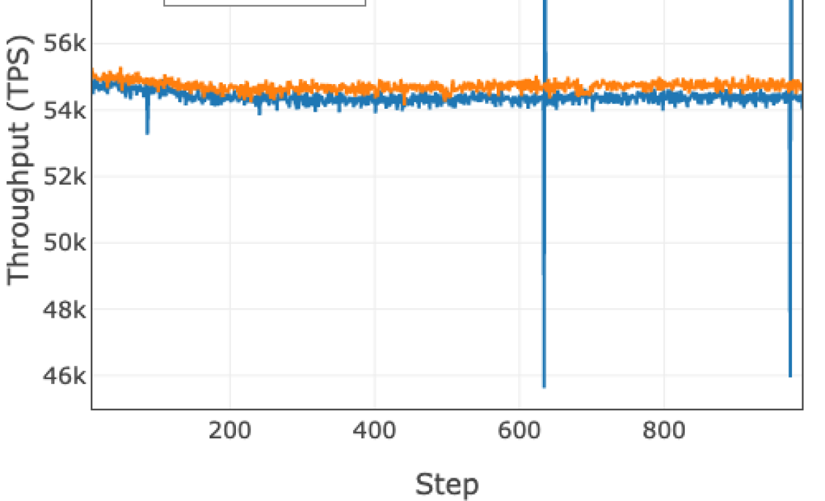
Figure 15: The training throughput in tokens per second (TPS) per device over the course of 1000 steps for two OLMo-1B models on 8 nodes, one with automatic garbage collection (GC), the other with collection done manually at intervals set within our training codebase. With automatic garbage collection, training throughput is slower and less stable, often becoming worse as the run progresses.

Explicit Python garbage collection

During training, the default Python garbage collector periodically runs a collection. In a distributed setting, with thousands of training processes that are expected to run in lock-step with each other, nothing enforces that these garbage collections happen at the same time on every process. Since distributed training can only proceed as fast as the slowest process, this causes a noticeable decrease in average training time per step as well as an increase in variability (Figure 15). Both worsen as the number of processes increases.

To work around this problem, the OLMo 2 trainer disables automatic garbage collection (e.g., by calling gc.disable()). Then, it runs garbage collection explicitly at regular intervals, triggered at the same time in each process (e.g. by calling gc.collect(1)).

Model Total GPU Power (MWh) Power Usage Effect. Carbon Intensity Carbon Emissions Water Usage Effect. Total Water Usage (kL) Llama 2 7B 74 1.1 - 31 1.29 - 4.26 105 - 347 Llama 3.1 8B 1,022 1.1 - 420 1.29 - 4.26 1,450 - 4,823 OLMo 7B 104 1.1 0.610 70 4.26 487 OLMo 2 7B 131 1.2 0.332 52 1.29 202 OLMo 2 13B 257 1.12 0.351 101 3.10 892

Table 19: CO₂ emissions and water consumption during pretraining. We estimate the total carbon emissions and water consumption for our new models using PUE information from our data center providers, carbon intensity data and WUE from the local grid for each data center, and total power consumption from time series data logged throughout training. Numbers for Llama 2 (Touvron et al., 2023), Llama 3 (Grattafiori et al., 2024), and the original OLMo (Groeneveld et al., 2024) are taken from their respective papers. We also show simulated water consumption for Llama 2 and 3, showing a range of water usage numbers using the lowest and highest WUE values for OLMo models.

6.5 Environmental Impact

Following our analysis in Groeneveld et al. (2024) and previous literature (Patterson et al., 2021; Dodge et al., 2022; Luccioni et al., 2022; Li et al., 2023a), we estimate the environmental impact of training our final models by first calculating the total energy consumed during pretraining, and multiplying it by the carbon intensity of the local grid to estimate the amount of carbon released. We additionally extend our previous analysis to also estimate water consumption, calculated by multiplying the power consumed by the water usage efficiency of both the power generation and the cooling hardware. As in Groeneveld et al. (2024), we emphasize that while our reporting is standard practice, it does not account for other environmental impacts such as embodied emissions and water consumption of the hardware during manufacturing, transportation, and eventual disposal, and other lifetime operational impacts such as deployment and inference, and thus our estimates should be viewed as lower bounds. We report detailed results for our models in Table 19.

As in Groeneveld et al. (2024), we calculate the total power consumption for each model by measuring the power consumption of an individual node every 25ms, calculating the average consumption throughout training, and multiplying by the total number of nodes. We then multiply this quantity by the power usage effectiveness (PUE) factor for the data center we use to train a model to account for the overall energy efficiency of the data center. As the majority of training for OLMo 2 7B is done on the Jupiter cluster, we use Jupiter’s efficiency metrics for our analysis of the 7B model. OLMo 2 13B is trained on Augusta; therefore, we use its efficiency metrics instead. We estimate consumption at about 391 MWh of energy by pretraining OLMo 2 7B and 13B.

To calculate carbon emissions, we multiply the total power consumption by a carbon intensity factor based on the physical location of each data center, measured in kg CO₂ per kWh. The Jupiter cluster is powered by Austin Energy, which most recently reported a carbon intensity of 0.332 kg CO₂ per kWh. The Augusta cluster is located in Iowa, and the state of Iowa has an average carbon intensity of 0.352 kg CO₂ per kWh, which we use for our calculations. We estimate that training our latest models emitted about 154 tCO₂eq.

$$CO_{2}\hskip 3.0pt\text{Emissions}=P_{\text{GPU}}\cdot\text{PUE}\cdot\text{Carbon Intensity}$$

To calculate water consumption, we multiply the total power consumption by the water usage effectiveness (WUE) of both the offsite power generation as well as the onsite cooling hardware. Both clusters use highly efficient, closed-loop cooling hardware, so we assume a WUE_onsite of 0 liters per kWh. Following Reig et al. (2020), we assume a WUE_offsite of 1.29 L per kWh for our Jupiter cluster and 3.10 L per kWh for our Augusta cluster. We estimate that training our latest models consumed about 1.1 million liters of water.

$$\text{Water Consumption}=P_{\text{GPU}}\cdot\text{PUE}\cdot(\text{WUE}_{\text{onsite}}+\text{WUE}_{\text{offsite}})$$

Though we aim to report a comprehensive analysis of the environmental impact of training our models, we emphasize that this is a lower bound on the total cost of developing large models. In an upcoming paper (Morrison et al., 2025), we will provide more comprehensive analysis covering energy, emissions, and water consumption throughout model development, pretraining, and deployment.

Conclusion

We introduce OLMo 2 and OLMo 2-Instruct, a family of fully open 7B and 13B parameter language models trained on up to 5T tokens. Both the base and instruct models are competitive with other open-weight models in their size categories such as Qwen 2.5, Gemma 2, and Llama 3.1. We detail the substantial contributions required to build competitive language models—many of which are different from the original OLMo—including stable infrastructure, architecture improvements for stability, innovations in late-stage training data, the latest post-training techniques, and many more details. We release all training and evaluation code, datasets, checkpoints, and logs required to reproduce and expand on the models. OLMo 2 marks continued progress in open-source language models, building a new ecosystem for research, one where new training methods and techniques need to be understood and shared.

Author Contributions

A successful team project like OLMo would not be possible without the fluid contributions of many teammates across formal team boundaries. As not all of these can be captured, we indicate each authors’ primary contributing role in OLMo 2. Authors are listed in alphabetical order:

• For base model development, including training and data curation: Shane Arora, Akshita Bhagia, Christopher Clark, Dirk Groeneveld, Yuling Gu, Matt Jordan, Jiacheng Liu, Kyle Lo, William Merrill, Tyler Murray, Dustin Schwenck, Luca Soldaini, Oyvind Tafjord, David Wadden, and Pete Walsh.

• For instruct model development, including training and data curation: Faeze Brahman, Pradeep Dasigi, Nouha Dziri, Yuling Gu, Shengyi Huang, Hamish Ivison, Nathan Lambert, Saumya Malik, Lester James V. Miranda, Jacob Morrison, Valentina Pyatkin, Oyvind Tafjord, and Christopher Wilhelm.

• For operational support, including program management, legal guidance, release process, and more: Taira Anderson, David Atkinson, Crystal Nam, and Aman Rangapur.

• For Ai2 cluster setup and support: Michal Guerquin, Michael Schmitz, Sam Skjonsberg, and Michael Wilson

• For mentorship and advising: Ali Farhadi, Hannaneh Hajishirzi, Pang Wei Koh, Noah A. Smith, and Luke Zettlemoyer.

Authorship for this work was determined by those making direct contributions to the OLMo 2 models, related artifacts, and their release. Core contributors are recognized for their sustained, significant contributions critical to the success of the OLMo 2 project.

Appendix A OLMo 2 Evaluation Framework

We evaluate OLMo 2 using OLMES, a unified, standardized evaluation suite and toolkit to guide the development and assess performance of language models.

OLMo base models are evaluated on 20 tasks, consisting of 10 multiple-choice tasks, 5 generative tasks, and 5 additional held-out tasks not utilized during model development. See Table 20 for the list of tasks along with details of the task formulations following the principles of the OLMES standard (Gu et al., 2024), described further below.

task	split	# inst (total)	# shots	metric	reference
Multiple-choice tasks
ARC-Challenge (ARC_C)	Test	1172	5	pmi	(Clark et al., 2018)
ARC-Easy (ARC_E)	Test	1000 (2376)	5	char	(Clark et al., 2018)
BoolQ	Val	1000 (3270)	5	none	(Clark et al., 2019)
CommonsenseQA (CSQA)	Val	1221	5	pmi	(Talmor et al., 2019)
HellaSwag (HSwag)	Val	1000 (10042)	5	char	(Zellers et al., 2019)
MMLU†	Test	14042	5	char	(Hendrycks et al., 2021)
OpenbookQA (OBQA)	Test	500	5	pmi	(Mihaylov et al., 2018)
PIQA	Val	1000 (1838)	5	char	(Bisk et al., 2020)
Social IQa (SIQA)	Val	1000 (1954)	5	char	(Sap et al., 2019)
WinoGrande (WinoG)	Val	1267	5	none	(Sakaguchi et al., 2020)
Generative tasks
CoQA	Val	7983	0	F1	(Reddy et al., 2019)
DROP	Val	1000 (9536)	5	F1	(Dua et al., 2019)
Jeopardy (JPRDY)	Test	2117	5	F1	(MosaicML, 2024)
Natural Questions (NatQs)	Val	1000 (3610)	5	F1	(Kwiatkowski et al., 2019)
SQuAD	Val	1000 (10570)	5	F1	(Rajpurkar et al., 2016)
Held-out tasks
AGIEval English	Test	2646	1	MCF	(Zhong et al., 2024)
BBH	Test	6511	3 (CoT)	EM	(Suzgun et al., 2022)
GSM8K	Test	1319	8 (CoT)	EM	(Cobbe et al., 2021)
MMLU-Pro	Test	12032	5	MCF	(Wang et al., 2024)
TriviaQA	Val	7993	5	F1	(Joshi et al., 2017)

Table 20: Details of OLMES benchmarks used in OLMo 2 evaluation, with standardized choices of dataset split, number of instances to use, along with total number if sampling was used. For multiple-choice tasks, when using the Cloze/Completion Formulation (CF), the “metric” column specifies which normalization scheme to use. Following the OLMES standard, we evaluate each model using both the MCF (Multiple-Choice Formulation) and CF formulations, and the best performing one is used. For efficiency reasons, we limit MMLU and held-out multiple-choice evaluations to MCF only as all the relevant models strongly prefer that format for these tasks.

Multiple-choice tasks

We use the formulation of the 10 multiple-choice tasks defined in the OLMES evaluation standard (Gu et al., 2024). OLMES (Open Language Model Evaluation Standard) is a set of principles and associated standard (with a reference implementation in the OLMES system framework) for reproducible LM evaluations that is open, practical, and documented, providing recommendations guided by experiments and results from the literature (Biderman et al., 2024; Gao et al., 2023). For multiple-choice tasks it is designed to support comparisons between smaller base models that require the cloze/completion formulation of multiple-choice questions (score each answer completion separately) against larger models that can utilize the multiple-choice formulation. To make our evaluations reproducible, we follow the OLMES standard in prompt formatting, choice of in-context examples, probability normalization, and all other details. See Table 20 and see Gu et al. (2024) for more details. Evaluation results on these tasks comparing OLMo 2 to other models can be found in Table 21.

Generative tasks

Following the principles of OLMES (Gu et al., 2024), such as prompt formatting and having 5-shot curated in-context examples, we also evaluated on a suite of generative tasks, OLMES-Gen. This suite covers factual knowledge tasks (Natural Questions (Kwiatkowski et al., 2019) and Jeopardy (MosaicML, 2024)) and tasks testing reading comprehension (SQuAD (Rajpurkar et al., 2016), DROP (Dua et al., 2019), and CoQA (Reddy et al., 2019)). For CoQA, the task comprises presenting a passage followed by a conversation so far, where each turn in the conversation contains a question and an answer. In this case, the previous question and answer pairs serve to guide the model in terms of the output format, and we do not include additional few-shot examples. For all other tasks, we follow OLMES in using 5-shot curated in-context examples. As the list of gold answers for these tasks are often incomplete, we use F1 as the primary metric to give partial credit when models produce answers that partially match. The task details of OLMES-Gen are summarized in Table 20. Evaluation results on the generative tasks are given in Table 22.

Held-out tasks

We also evaluate on a held-out suite of tasks that were not used when making decisions during model development. This suite includes advanced admission and qualification exams (AGIEval English (Zhong et al., 2024)), tasks believed to be challenging to LMs (BigBenchHard, BBH; Suzgun et al., 2022), math reasoning (GSM8K; Cobbe et al., 2021), a more challenging and reasoning-focused extension of MMLU (MMLU Pro; Wang et al., 2024), and an unseen factual knowledge task (TriviaQA; Joshi et al., 2017). We use existing in-context examples where available - for GSM8K, we use the 8-shot CoT examples from Wei et al. (2023); for BBH we use the 3-shot CoT prompts from the original dataset; in evaluating MMLU-Pro, we used 5-shot examples from the original dataset. We use a 1-shot (with passage context, no CoT) prompt for AGIEval English, and a manually curated 5-shot examples from the train set for TriviaQA. Note that for the case of GSM8K, we never evaluated our models on the entire test set during the development stage, instead we use 200 examples to inform choices during development (e.g., choices of annealing mixtures); in Section 4 we refer to this 200-example subset as GSM*. Evaluation results on the held-out tasks can be found in Table 23.

We make all implementations publicly available at github.com/allenai/olmes.

Model	Avg	ARC_C	ARC_E	BoolQ	CSQA	HSwag	OBQA	PIQA	SIQA	WinoG
Open weights models
Llama-2-13B	76.0	$67.3^{\dagger}$	85.9	86.7	74.0	83.9	$65.4^{\dagger}$	80.2	$65.9^{\dagger}$	74.9
Llama-3.1-8B	80.4	$79.5^{\dagger}$	$91.7^{\dagger}$	88.5	$74.3^{\dagger}$	81.6	$78.6^{\dagger}$	81.1	$71.4^{\dagger}$	76.6
Mistral-7B-v0.3	80.5	$78.3^{\dagger}$	$91.1^{\dagger}$	88.4	$72.7^{\dagger}$	83.1	$80.0^{\dagger}$	81.9	$71.2^{\dagger}$	77.7
Mistral-Nemo-Bs-12B	83.9	$85.2^{\dagger}$	$93.7^{\dagger}$	90.5	$77.0^{\dagger}$	85.6	$83.2^{\dagger}$	$86.2^{\dagger}$	$72.2^{\dagger}$	81.5
Gemma-2-9B	85.5	$89.5^{\dagger}$	$95.5^{\dagger}$	89.4	$78.8^{\dagger}$	$87.3^{\dagger}$	$88.4^{\dagger}$	$86.1^{\dagger}$	$76.0^{\dagger}$	78.8
Qwen-2.5-7B	86.8	$89.5^{\dagger}$	$96.1^{\dagger}$	89.3	$86.0^{\dagger}$	$89.7^{\dagger}$	$90.2^{\dagger}$	$87.7^{\dagger}$	$78.1^{\dagger}$	74.2
Qwen-2.5-14B	90.0	$94.0^{\dagger}$	$98.2^{\dagger}$	$90.9^{\dagger}$	$86.6^{\dagger}$	$94.0^{\dagger}$	$94.8^{\dagger}$	$90.8^{\dagger}$	$81.1^{\dagger}$	80.0
Models with partially available data
StableLM-2-12B	83.8	$81.9^{\dagger}$	$91.8^{\dagger}$	90.0	$83.1^{\dagger}$	84.5	$81.4^{\dagger}$	$86.6^{\dagger}$	$77.1^{\dagger}$	77.7
Zamba-2-7B	86.6	$92.2^{\dagger}$	$96.7^{\dagger}$	89.3	$84.0^{\dagger}$	$89.4^{\dagger}$	$84.2^{\dagger}$	$86.5^{\dagger}$	$77.7^{\dagger}$	79.6
Fully-open models
Amber-7B	65.6	44.9	77.5	72.5	70.9	74.5	51.0	77.9	56.1	65.5
OLMo-7B	68.0	46.4	78.9	78.7	70.8	78.1	55.8	78.5	56.5	68.5
OLMo-0424-7B	77.9	$66.9^{\dagger}$	$83.6^{\dagger}$	85.9	$85.8^{\dagger}$	80.1	$68.6^{\dagger}$	80.3	$76.1^{\dagger}$	73.6
MAP-Neo-7B	78.4	$78.4^{\dagger}$	$90.6^{\dagger}$	86.8	$82.1^{\dagger}$	72.8	$74.4^{\dagger}$	77.3	$73.6^{\dagger}$	69.2
DCLM-7B	80.7	$79.8^{\dagger}$	$92.3^{\dagger}$	87.0	77.0	82.3	$79.6^{\dagger}$	80.1	$71.2^{\dagger}$	77.3
OLMo-2-1124-7B	80.9	$79.8^{\dagger}$	$90.8^{\dagger}$	86.3	75.1	83.8	$80.4^{\dagger}$	80.6	$74.1^{\dagger}$	77.2
OLMo-2-1124-13B	83.9	$83.5^{\dagger}$	$93.7^{\dagger}$	87.9	$77.9^{\dagger}$	86.4	$84.4^{\dagger}$	83.8	$75.6^{\dagger}$	81.5

Table 21: Results on 9 multiple-choice tasks from the OLMES standard, where $\dagger$ indicates that the MCF (multiple-choice) formulation was used rather than CF (cloze). See Appendix D for the separate MCF and CF scores.

Model	Avg	MMLU	CoQA	DROP	JPRDY	NatQs	SQuAD
Open weights models
Qwen-2.5-7B	62.0	74.4	48.3	55.8	77.5	29.9	86.0
Qwen-2.5-14B	63.2	79.3	41.1	51.5	82.4	37.3	87.2
Mistral-7B-v0.3	63.4	63.5	58.5	51.8	80.4	37.2	88.8
Llama-2-13B	64.4	55.7	77.4	45.6	81.4	38.4	87.7
Mistral-Nemo-Base-12B	67.0	69.5	49.0	69.2	83.6	39.7	90.8
Llama-3.1-8B	68.2	66.9	82.0	56.4	80.5	33.9	89.6
Gemma-2-9B	71.1	70.6	83.3	63.0	83.5	38.0	88.0
Models with partially available data
Zamba-2-7B	63.4	68.5	51.3	51.7	82.2	36.5	90.4
StableLM-2-12B	67.4	62.4	80.8	55.5	80.7	37.6	87.0
Fully-open models
Amber-7B	46.3	24.7	70.7	26.1	62.4	18.7	75.4
OLMo-7B	49.8	28.3	73.6	27.3	66.9	24.8	77.9
OLMo-0424-7B	57.4	54.3	65.6	50.0	67.7	29.6	77.2
MAP-Neo-7B	59.3	58.0	69.0	39.4	72.8	28.9	87.6
DCLM-7B	63.0	64.4	79.1	39.3	78.5	28.8	87.9
OLMo-2-1124-7B	69.3	63.7	80.8	60.8	80.9	36.9	92.6
OLMo-2-1124-13B	74.6	67.5	85.9	70.7	83.0	46.7	94.0

Table 22: Results on MMLU and the OLMES-Gen suite of 5 generative tasks tracked during model development.

Model	Avg	AGIEval	BBH	GSM8k	MMLU-Pro	TriviaQA
Open weights models
Llama-2-13B	44.5	41.5	47.5	28.1	23.9	81.3
Mistral-7B-v0.3	50.9	47.3	57.7	40.1	30.0	79.3
Llama-3.1-8B	57.2	51.3	63.2	56.5	34.7	80.3
Mistral-Nemo-Base-2407-12B	61.3	54.7	68.3	62.1	36.7	84.6
Gemma-2-9B	63.4	57.3	65.7	70.1	42.0	81.8
Qwen-2.5-7B	65.8	63.7	68.4	81.5	45.8	69.4
Qwen-2.5-14B	72.3	71.0	75.2	83.4	52.8	79.1
Models with partially available data
StableLM-2-12B	55.9	50.9	57.2	62.0	29.3	79.9
Zamba-2-7B	58.0	55.5	55.6	67.2	32.8	78.8
Fully-open models
Amber-7B	25.7	21.8	31.0	4.8	11.7	59.3
OLMo-7B	28.1	23.7	31.4	9.2	12.1	64.1
OLMo-0424-7B	37.2	43.9	33.4	27.7	22.1	58.8
MAP-Neo-7B	38.1	45.8	41.4	12.5	25.9	65.1
DCLM-7B	49.5	47.5	50.4	46.1	31.3	72.1
OLMo-2-1124-7B	55.3	50.4	49.8	67.5	31.0	78.0
OLMo-2-1124-13B	60.5	54.2	56.3	75.1	35.1	81.9

Table 23: Results on held-out tasks not tracked during model development.

Appendix B Additional Instruct Details

B.1 Additional Hyperparameters

All of the models used to generate preference data for OLMo 2-Instruct are listed in Table 25. The prompt sources for the preference datasets are listed in Table 27 – for more information on their contents, refer to Lambert et al. (2024). The hyperparameters used to train the reward models for RLVR value network initialization are shown in Table 26.

B.2 Additional RLVR Learning Curves

The additional 13B RLVR learning curves of can be found at Figure 17, Figure 18, and Figure 19.

B.3 OLMo 2-Instruct Preview Models

We made an initial release prior to this report. However, soon after the release, a tokenizer issue came to our attention: Our base model’s pre-tokenization logic differs from our instruct model’s tokenizer.

Specifically, the OLMo-2 base models utilized the GPT2Tokenizer tokenizer class, with custom pre-tokenization logic (e.g., on splitting or truncating sequences), which is lost during the instruct model’s training. Figure 16 shows the filediff between the base model’s tokenizer.json and the instruct model’s tokenizer.json.

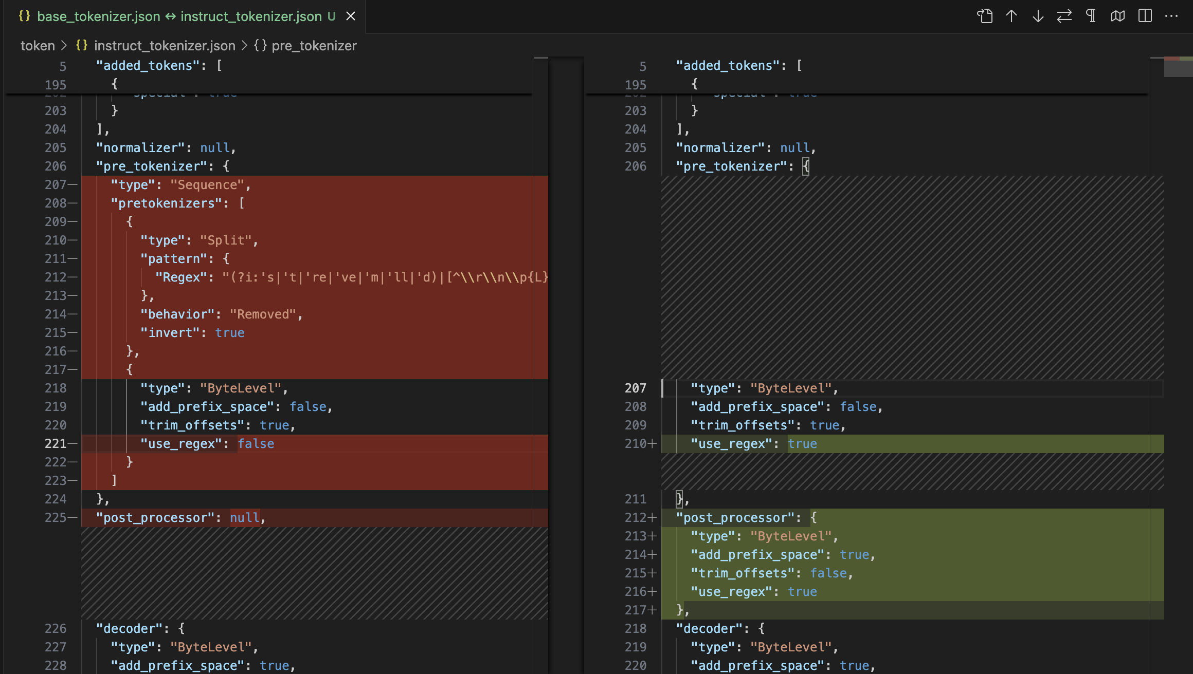
Figure 16: The file diff between the OLMo 2-Instruct and OLMo 2-Instruct Preview’s tokenizer.json: the pre-tokenization logic is lost during OLMo 2-Instruct Preview’s training, so we have decided to re-train OLMo 2-Instruct models.

Because of this, we have decided to retrain our OLMo 2-Instruct models to be consistent with our base models and mark the existing post-trained models as preview models.

Nevertheless, the OLMo 2-Instruct Preview learning curves can be found at Figure 20 and Figure 21.

OLMo-2-1124-13B-RLVR1

Figure 17: The top row shows the training curves of OLMo-2-1124-13B-RLVR1 showing verifiable rewards, KL divergence, and response lengths. The bottom row shows the corresponding downstream evaluations and the average scores across our evaluation suites.

OLMo-2-1124-13B-RLVR2

Figure 18: The top row shows the training curves of OLMo-2-1124-13B-RLVR2 showing verifiable rewards, KL divergence, and response lengths. The solid lines in the bottom row show the corresponding downstream evaluation and the average scores across our evaluation suites.

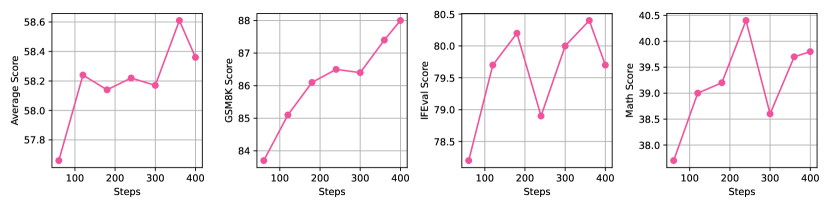
OLMo-2-1124-13B-Instruct

Figure 19: The top row shows the training curves of OLMo-2-1124-13B-Instruct showing verifiable rewards, KL divergence, and response lengths. The solid lines in the bottom row show the corresponding downstream evaluation and the average scores across our evaluation suites.

OLMo-2-1124-13B-Instruct-Preview

Figure 20: The OLMo-2-1124-13B-Instruct-Preview results. The top row shows the training curves of OLMo-2-1124-7B-Instruct on verifiable rewards, KL divergence, and response lengths. In the bottom row, the y-axes show the average scores across our evaluation suites and GSM8K scores. Overall, RLVR increases both training rewards and evaluation scores.

OLMo-2-1124-7B-Instruct-Preview

Figure 21: The top row shows the training curves of OLMo-2-1124-13B-Instruct-Preview on verifiable rewards, KL divergence, and response lengths. In the bottom row, the y-axes show the average scores across our evaluation suites and GSM8K, IFEval, and MATH Flex scores, respectively. Overall, we found RLVR increases not only the training rewards of our 13B models but also the downstream evaluations such as GSM8K.

		AGI Eval	DeepMind
Model	Average	English	Math	GPQA	IFEval OOD	MMLU Pro
OLMo 2 1124 13B Inst.	35.10	60.5	26.8	28.8	18.0	41.4
OLMo 2 1124 13B DPO	35.18	60.1	25.4	32.1	16.5	41.8
OLMo 2 1124 13B SFT	32.68	56.0	27.1	27.0	15.1	38.2
OLMo 2 1124 7B Inst.	32.08	57.2	19.1	30.1	18.0	36.0
OLMo 2 1124 7B DPO	31.70	56.7	17.7	30.6	16.9	36.6
OLMo 2 1124 7B SFT	29.26	52.7	19.0	27.7	13.7	33.2
OLMo 7B 0724 Inst.	22.92	43.6	5.8	27.9	14.4	22.9
OLMoE 1B 7B 0924 Inst.	20.54	39.1	4.2	27.5	11.3	20.6

Table 24: Evaluation results for OLMo Instruct models on the unseen suite from Lambert et al. (2024).

Appendix C Additional Hyperparameters

The models used for the on-policy preference data generation are listed in Table 25.

Model Name	Reference
Yi-34B-Chat	(Young et al., 2024)
Yi-6B-Chat	(Young et al., 2024)
Tülu 2 7B	(Ivison et al., 2023)
Tülu 2 13B	(Ivison et al., 2023)
Google Gemma 2 27B it	(Gemma Team et al., 2024b)
Google Gemma 2 9B it	(Gemma Team et al., 2024b)
GPT-4o	(Hurst et al., 2024)
MPT 30B Chat	(MosaicML NLP Team, 2023)
MPT 7B 8k Chat	(MosaicML NLP Team, 2023)
Mistral 7B Instruct v0.2	(Jiang et al., 2023)
Mistral Nemo Instruct 2407	(Mistral AI, 2024)
Qwen2.5 32B Instruct	(Qwen et al., 2024)
Qwen2.5 14B Instruct	(Qwen et al., 2024)
Qwen 2.5 7B Instruct	(Qwen et al., 2024)
Falcon 7B	(Almazrouei et al., 2023)
SmolLM2 1.7B Instruct	(Allal et al., 2024b)
Phi 3 Mini 128k Instruct	(Abdin et al., 2024a)
Phi 3.5 Mini Instruct	(Abdin et al., 2024a)
NuExtract-1.5	(Numind, 2024)

Table 25: External models used to sample off-policy data in the synthetic preference pipeline. These are in addition to the on-policy samples from the SFT checkpoints.

Hyperparameter	Value
Learning Rate	$3\cdot 10^{-6}$
Gradient Norm Threshold	1.0
Learning Rate Schedule	Linear
Batch Size (effective)	256
Max Token Length	2,048
Number of Epochs	1

Table 26: This table shows the hyperparameters used to train the reward model for RLVR value network initialization.

Dataset	Counts	7B DPO	13B DPO
SFT Reused	117,025	$\checkmark$	$\checkmark$
SFT IF	65,792	$\checkmark$	$\checkmark$
WildChat Unused	84,105	$\checkmark$	$\checkmark$
WildChat Reused	17,703	$\checkmark$	$\checkmark$
WildChat IF	10,794		$\checkmark$
Ultrafeedback (cleaned)	60,816	$\checkmark$	$\checkmark$
DaringAnteater IF	1,618	$\checkmark$	$\checkmark$
Tülu 3 Personas IF	19,890	$\checkmark$	$\checkmark$
Total	377,743

Table 27: Prompt sources for preference finetuning datasets.

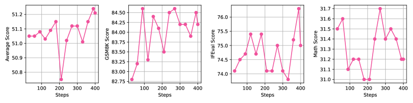
OLMo 2 7B Instruct Preview (alternative)

Figure 22: The top row shows the training curves of OLMo-2-1124-13B-Instruct on verifiable rewards, KL divergence, and response lengths. In the bottom row, the y-axes show the average scores across our evaluation suites and GSM8K, IFEval, and MATH Flex scores, respectively. Overall, we found RLVR increases not only the training rewards of our 13B models but also the downstream evaluations such as GSM8K.

Appendix D Additional Evaluation Results

D.1 Base Models

In Tables 28 and 29 we show the separate MCF (multiple-choice) and CF (cloze) formulation scores for the 9 OLMES tasks shown (using the maximum per task) in Table 21.

Model	Avg	ARC_C	ARC_E	BoolQ	CSQA	HSwag	OBQA	PIQA	SIQA	WinoG
Open weights models
Llama-2-13B	69.1	67.3	85.0	77.8	68.1	62.4	65.4	74.0	65.9	56.1
Mistral-7B-v0.3	76.0	78.3	91.1	88.2	72.7	67.6	80.0	76.8	71.2	58.5
Llama-3.1-8B	76.4	79.5	91.7	84.5	74.3	67.7	78.6	78.3	71.4	61.4
Mistral-Nemo-Base-12B	80.8	85.2	93.7	89.2	77.0	71.8	83.2	86.2	72.2	69.0
Gemma-2-9B	84.4	89.5	95.5	88.6	78.8	87.3	88.4	86.1	76.0	69.7
Qwen-2.5-7B	86.0	89.5	96.1	88.3	86.0	89.7	90.2	87.7	78.1	68.1
Qwen-2.5-14B	89.7	94.0	98.2	90.9	86.6	94.0	94.8	90.8	81.1	77.1
Models with partially available data
StableLM-2-12B	82.1	81.9	91.8	88.0	83.1	81.3	81.4	86.6	77.1	67.2
Zamba-2-7B	85.5	92.2	96.7	89.0	84.0	89.4	84.2	86.5	77.7	69.7
Fully-open models
Amber-7B	37.4	28.0	30.9	63.8	22.8	27.9	27.6	50.2	35.6	49.6
OLMo-7B	37.5	27.2	27.0	67.5	20.8	25.0	27.0	57.2	35.1	50.4
OLMo-0424-7B	70.5	66.9	83.6	82.0	85.8	50.0	68.6	65.6	76.1	56.2
MAP-Neo-7B	76.0	78.4	90.6	85.0	82.1	68.7	74.4	74.9	73.6	56.4
DCLM-7B	77.4	79.8	92.3	83.3	75.7	77.4	79.6	78.7	71.2	59.0
OLMo-2-1124-7B	77.9	79.8	90.8	83.8	72.9	75.2	80.4	78.1	74.1	65.7
OLMo-2-1124-13B	81.6	83.5	93.7	83.3	77.9	84.5	84.4	81.1	75.6	70.1

Table 28: Results on 9 OLMES multiple-choice tasks using the MCF (multiple-choice) formulation only.

Model	Avg	ARC_C	ARC_E	BoolQ	CSQA	HSwag	OBQA	PIQA	SIQA	WinoG
Open weights models
Gemma-2-9B	73.4	57.5	89.4	89.4	62.6	83.1	56.4	82.1	61.8	78.8
Llama-3.1-8B	73.9	57.3	86.6	88.5	72.0	81.6	57.6	81.1	63.4	76.6
Llama-2-13B	74.0	56.2	85.9	86.7	74.0	83.9	60.8	80.2	63.6	74.9
Mistral-7B-v0.3	74.6	59.0	86.5	88.4	72.0	83.1	61.0	81.9	61.9	77.7
Qwen-2.5-7B	75.5	63.1	87.9	89.3	76.5	81.1	65.4	78.5	63.3	74.2
Mistral-Nemo-Base-2407-12B	76.6	63.8	88.2	90.5	74.5	85.6	61.2	82.1	62.0	81.5
Qwen-2.5-14B	78.3	68.1	89.7	90.0	77.3	84.9	67.8	82.1	64.4	80.0
Models with partially available data
StableLM-2-12B	75.7	59.0	84.5	90.0	76.6	84.5	63.8	80.2	65.1	77.7
Zamba-2-7B	77.1	67.2	88.4	89.3	74.0	85.6	65.4	81.7	63.0	79.6
Fully-open models
Amber-7B	65.6	44.9	77.5	72.5	70.9	74.5	51.0	77.9	56.1	65.5
OLMo-7B	68.0	46.4	78.9	78.7	70.8	78.1	55.8	78.5	56.5	68.5
MAP-Neo-7B	68.8	48.4	82.3	86.8	64.3	72.8	55.8	77.3	62.1	69.2
OLMo-0424-7B	70.9	51.2	81.5	85.9	70.4	80.1	59.8	80.3	54.9	73.6
DCLM-7B	75.1	61.5	86.6	87.0	77.0	82.3	62.4	80.1	62.0	77.3
OLMo-2-1124-7B	75.3	60.2	87.0	86.3	75.1	83.8	64.6	80.6	63.0	77.2
OLMo-2-1124-13B	77.6	63.9	88.5	87.9	76.7	86.4	66.4	83.8	63.1	81.5

Table 29: Results on 9 OLMES multiple-choice tasks using the CF (cloze) formulation only.

D.2 Instruct Models

The evaluations of OLMo 2-Instruct models on the Tülu 3 Unseen evaluation suite, minus coding tasks that are out of scope, are shown in Table 24.

Appendix E Annealing Data Details

Figure 23: Prompt used to generate hard math word problems. {persona} are borrowed from Chan et al. (2024).

Figure 24: Prompt used to generate solutions for hard math word problems.

References

- Abdin et al. (2024a) M. Abdin, J. Aneja, H. Awadalla, A. Awadallah, A. A. Awan, N. Bach, A. Bahree, A. Bakhtiari, J. Bao, H. Behl, et al. Phi-3 technical report: A highly capable language model locally on your phone. arXiv preprint arXiv:2404.14219, 2024a.
- Abdin et al. (2024b) M. Abdin, J. Aneja, H. S. Behl, S. Bubeck, R. Eldan, S. Gunasekar, M. Harrison, R. J. Hewett, M. Javaheripi, P. Kauffmann, J. R. Lee, Y. T. Lee, Y. Li, W. Liu, C. C. T. Mendes, A. Nguyen, E. Price, G. de Rosa, O. Saarikivi, A. Salim, S. Shah, X. Wang, R. Ward, Y. Wu, D. Yu, C. Zhang, and Y. Zhang. Phi-4 technical report. arXiv preprint arXiv:2412.08905, 2024b.
- Ai2 (2024) Ai2. OLMo-1.7 7B: A 24-point improvement on MMLU, 4 2024. URL https://allenai.org/blog/olmo-1-7-7b-a-24-point-improvement-on-mmlu-92b43f7d269d.
- Akter et al. (2024) S. N. Akter, S. Prabhumoye, J. Kamalu, S. Satheesh, E. Nyberg, M. Patwary, M. Shoeybi, and B. Catanzaro. Mind: Math informed synthetic dialogues for pretraining llms, 2024. URL https://arxiv.org/abs/2410.12881.
- Allal et al. (2024a) L. B. Allal, A. Lozhkov, and E. Bakouch. Smollm - blazingly fast and remarkably powerful, 07 2024a.
- Allal et al. (2024b) L. B. Allal, A. Lozhkov, E. Bakouch, G. M. Blázquez, L. Tunstall, A. Piqueres, A. Marafioti, C. Zakka, L. von Werra, and T. Wolf. Smollm2 - with great data, comes great performance, 11 2024b.
- Almazrouei et al. (2023) E. Almazrouei, H. Alobeidli, A. Alshamsi, A. Cappelli, R. Cojocaru, M. Debbah, E. Goffinet, D. Heslow, J. Launay, Q. Malartic, B. Noune, B. Pannier, and G. Penedo. Falcon-40B: an open large language model with state-of-the-art performance. 2023.
- Ansel et al. (2024) J. Ansel, E. Yang, H. He, N. Gimelshein, A. Jain, M. Voznesensky, B. Bao, P. Bell, D. Berard, E. Burovski, G. Chauhan, A. Chourdia, W. Constable, A. Desmaison, Z. DeVito, E. Ellison, W. Feng, J. Gong, M. Gschwind, B. Hirsh, S. Huang, K. Kalambarkar, L. Kirsch, M. Lazos, M. Lezcano, Y. Liang, J. Liang, Y. Lu, C. K. Luk, B. Maher, Y. Pan, C. Puhrsch, M. Reso, M. Saroufim, M. Y. Siraichi, H. Suk, S. Zhang, M. Suo, P. Tillet, X. Zhao, E. Wang, K. Zhou, R. Zou, X. Wang, A. Mathews, W. Wen, G. Chanan, P. Wu, and S. Chintala. Pytorch 2: Faster machine learning through dynamic python bytecode transformation and graph compilation. In Proceedings of the 29th ACM International Conference on Architectural Support for Programming Languages and Operating Systems, Volume 2, ASPLOS ’24, page 929–947, New York, NY, USA, 2024. Association for Computing Machinery. ISBN 9798400703850. 10.1145/3620665.3640366. URL https://doi.org/10.1145/3620665.3640366.
- Antoniades et al. (2024) A. Antoniades, X. Wang, Y. Elazar, A. Amayuelas, A. Albalak, K. Zhang, and W. Y. Wang. Generalization v.s. memorization: Tracing language models’ capabilities back to pretraining data. ArXiv, abs/2407.14985, 2024. URL https://api.semanticscholar.org/CorpusID:271328219.
- Azerbayev et al. (2023) Z. Azerbayev, H. Schoelkopf, K. Paster, M. D. Santos, S. McAleer, A. Q. Jiang, J. Deng, S. Biderman, and S. Welleck. Llemma: An open language model for mathematics, 2023.
- Ba et al. (2016) J. Ba, J. R. Kiros, and G. E. Hinton. Layer normalization. ArXiv, abs/1607.06450, 2016. URL https://api.semanticscholar.org/CorpusID:8236317.
- Bhagia et al. (2024) A. Bhagia, J. Liu, A. Wettig, D. Heineman, O. Tafjord, A. H. Jha, L. Soldaini, N. A. Smith, D. Groeneveld, P. W. Koh, J. Dodge, and H. Hajishirzi. Establishing task scaling laws via compute-efficient model ladders, 2024. URL https://arxiv.org/abs/2412.04403.
- Biderman et al. (2023) S. Biderman, H. Schoelkopf, Q. G. Anthony, H. Bradley, K. O’Brien, E. Hallahan, M. A. Khan, S. Purohit, U. S. Prashanth, E. Raff, et al. Pythia: A suite for analyzing large language models across training and scaling. In International Conference on Machine Learning, pages 2397–2430. PMLR, 2023.
- Biderman et al. (2024) S. Biderman, H. Schoelkopf, L. Sutawika, L. Gao, J. Tow, B. Abbasi, A. F. Aji, P. S. Ammanamanchi, S. Black, J. Clive, A. DiPofi, J. Etxaniz, B. Fattori, J. Z. Forde, C. Foster, M. Jaiswal, W. Y. Lee, H. Li, C. Lovering, N. Muennighoff, E. Pavlick, J. Phang, A. Skowron, S. Tan, X. Tang, K. A. Wang, G. I. Winata, F. Yvon, and A. Zou. Lessons from the trenches on reproducible evaluation of language models. arXiv:2405.14782, 2024.
- Bisk et al. (2020) Y. Bisk, R. Zellers, R. Le bras, J. Gao, and Y. Choi. PIQA: Reasoning about physical commonsense in natural language. Proceedings of the AAAI Conference on Artificial Intelligence, 34(05):7432–7439, Apr. 2020. 10.1609/aaai.v34i05.6239. URL https://ojs.aaai.org/index.php/AAAI/article/view/6239.
- Black et al. (2022) S. Black, S. Biderman, E. Hallahan, Q. Anthony, L. Gao, L. Golding, H. He, C. Leahy, K. McDonell, J. Phang, M. Pieler, U. S. Prashanth, S. Purohit, L. Reynolds, J. Tow, B. Wang, and S. Weinbach. GPT-NeoX-20B: An open-source autoregressive language model. In Proceedings of the ACL Workshop on Challenges & Perspectives in Creating Large Language Models, 2022. URL https://arxiv.org/abs/2204.06745.
- Blakeney et al. (2024) C. Blakeney, M. Paul, B. W. Larsen, S. Owen, and J. Frankle. Does your data spark joy? performance gains from domain upsampling at the end of training, 2024. URL https://arxiv.org/abs/2406.03476.
- Chameleon Team (2024) Chameleon Team. Chameleon: Mixed-modal early-fusion foundation models. ArXiv, abs/2405.09818, 2024. URL https://api.semanticscholar.org/CorpusID:269791516.
- Chan et al. (2024) X. Chan, X. Wang, D. Yu, H. Mi, and D. Yu. Scaling synthetic data creation with 1,000,000,000 personas. arXiv preprint arXiv:2406.20094, 2024.
- Chang et al. (2024) H. Chang, J. Park, S. Ye, S. Yang, Y. Seo, D.-S. Chang, and M. Seo. How do large language models acquire factual knowledge during pretraining? arXiv preprint arXiv:2406.11813, 2024.
- Chowdhery et al. (2022) A. Chowdhery, S. Narang, J. Devlin, M. Bosma, G. Mishra, A. Roberts, P. Barham, H. W. Chung, C. Sutton, S. Gehrmann, P. Schuh, K. Shi, S. Tsvyashchenko, J. Maynez, A. Rao, P. Barnes, Y. Tay, N. M. Shazeer, V. Prabhakaran, E. Reif, N. Du, B. Hutchinson, R. Pope, J. Bradbury, J. Austin, M. Isard, G. Gur-Ari, P. Yin, T. Duke, A. Levskaya, S. Ghemawat, S. Dev, H. Michalewski, X. García, V. Misra, K. Robinson, L. Fedus, D. Zhou, D. Ippolito, D. Luan, H. Lim, B. Zoph, A. Spiridonov, R. Sepassi, D. Dohan, S. Agrawal, M. Omernick, A. M. Dai, T. S. Pillai, M. Pellat, A. Lewkowycz, E. Moreira, R. Child, O. Polozov, K. Lee, Z. Zhou, X. Wang, B. Saeta, M. Díaz, O. Firat, M. Catasta, J. Wei, K. S. Meier-Hellstern, D. Eck, J. Dean, S. Petrov, and N. Fiedel. Palm: Scaling language modeling with pathways. ArXiv, abs/2204.02311, 2022. URL https://api.semanticscholar.org/CorpusID:247951931.
- Clark et al. (2019) C. Clark, K. Lee, M.-W. Chang, T. Kwiatkowski, M. Collins, and K. Toutanova. BoolQ: Exploring the surprising difficulty of natural yes/no questions. In J. Burstein, C. Doran, and T. Solorio, editors, Proceedings of the 2019 Conference of the North American Chapter of the Association for Computational Linguistics: Human Language Technologies, Volume 1 (Long and Short Papers), pages 2924–2936, Minneapolis, Minnesota, June 2019. Association for Computational Linguistics. 10.18653/v1/N19-1300. URL https://aclanthology.org/N19-1300.
- Clark et al. (2018) P. Clark, I. Cowhey, O. Etzioni, T. Khot, A. Sabharwal, C. Schoenick, and O. Tafjord. Think you have solved question answering? Try ARC, the AI2 reasoning challenge. CoRR, arXiv:1803.05457, 2018.
- Cobbe et al. (2021) K. Cobbe, V. Kosaraju, M. Bavarian, M. Chen, H. Jun, L. Kaiser, M. Plappert, J. Tworek, J. Hilton, R. Nakano, C. Hesse, and J. Schulman. Training verifiers to solve math word problems, 2021. URL https://arxiv.org/abs/2110.14168.
- Cohere (2024a) Cohere. Command R: Retrieval-Augmented Generation at Production Scale. https://cohere.com/blog/command-r, 2024a. Accessed: 2024-12-17.
- Cohere (2024b) Cohere. Introducing Command R7B: Fast and efficient generative AI. https://cohere.com/blog/command-r7b, 2024b. Accessed: 2024-12-17.
- Cohere (2024c) Cohere. Introducing Command R+: A Scalable LLM Built for Business. https://cohere.com/blog/command-r-plus-microsoft-azure, 2024c. Accessed: 2024-12-17.
- Cottier et al. (2024) B. Cottier, J. You, N. Martemianova, and D. Owen. How far behind are open models?, Nov. 2024. URL https://epoch.ai/blog/open-models-report. Accessed: 2024-12-18.
- Cowsik et al. (2024) A. Cowsik, T. Nebabu, X.-L. Qi, and S. Ganguli. Geometric dynamics of signal propagation predict trainability of transformers, 2024. URL https://arxiv.org/abs/2403.02579.
- Cui et al. (2023) G. Cui, L. Yuan, N. Ding, G. Yao, W. Zhu, Y. Ni, G. Xie, Z. Liu, and M. Sun. Ultrafeedback: Boosting language models with high-quality feedback. arXiv preprint arXiv:2310.01377, 2023.
- Dao (2024) T. Dao. FlashAttention-2: Faster attention with better parallelism and work partitioning. In International Conference on Learning Representations (ICLR), 2024.
- Databricks (2024) Databricks. Introducing DBRX: A New State-of-the-Art Open LLM, 3 2024. URL https://www.databricks.com/blog/introducing-dbrx-new-state-art-open-llm.
- Dehghani et al. (2023a) M. Dehghani, J. Djolonga, B. Mustafa, P. Padlewski, J. Heek, J. Gilmer, A. Steiner, M. Caron, R. Geirhos, I. Alabdulmohsin, R. Jenatton, L. Beyer, M. Tschannen, A. Arnab, X. Wang, C. Riquelme, M. Minderer, J. Puigcerver, U. Evci, M. Kumar, S. van Steenkiste, G. F. Elsayed, A. Mahendran, F. Yu, A. Oliver, F. Huot, J. Bastings, M. P. Collier, A. Gritsenko, V. Birodkar, C. Vasconcelos, Y. Tay, T. Mensink, A. Kolesnikov, F. Pavetić, D. Tran, T. Kipf, M. Lučić, X. Zhai, D. Keysers, J. Harmsen, and N. Houlsby. Scaling vision transformers to 22 billion parameters, 2023a. URL https://arxiv.org/abs/2302.05442.
- Dehghani et al. (2023b) M. Dehghani, J. Djolonga, B. Mustafa, P. Padlewski, J. Heek, J. Gilmer, A. Steiner, M. Caron, R. Geirhos, I. M. Alabdulmohsin, R. Jenatton, L. Beyer, M. Tschannen, A. Arnab, X. Wang, C. Riquelme, M. Minderer, J. Puigcerver, U. Evci, M. Kumar, S. van Steenkiste, G. F. Elsayed, A. Mahendran, F. Yu, A. Oliver, F. Huot, J. Bastings, M. Collier, A. A. Gritsenko, V. Birodkar, C. N. Vasconcelos, Y. Tay, T. Mensink, A. Kolesnikov, F. Paveti’c, D. Tran, T. Kipf, M. Luvci’c, X. Zhai, D. Keysers, J. Harmsen, and N. Houlsby. Scaling vision transformers to 22 billion parameters. ArXiv, abs/2302.05442, 2023b. URL https://api.semanticscholar.org/CorpusID:256808367.
- Dodge et al. (2022) J. Dodge, T. Prewitt, R. T. D. Combes, E. Odmark, R. Schwartz, E. Strubell, A. S. Luccioni, N. A. Smith, N. DeCario, and W. Buchanan. Measuring the carbon intensity of ai in cloud instances, 2022. URL https://arxiv.org/abs/2206.05229.
- Dua et al. (2019) D. Dua, Y. Wang, P. Dasigi, G. Stanovsky, S. Singh, and M. Gardner. DROP: A reading comprehension benchmark requiring discrete reasoning over paragraphs. In J. Burstein, C. Doran, and T. Solorio, editors, Proceedings of the 2019 Conference of the North American Chapter of the Association for Computational Linguistics: Human Language Technologies, Volume 1 (Long and Short Papers), pages 2368–2378, Minneapolis, Minnesota, June 2019. Association for Computational Linguistics. 10.18653/v1/N19-1246. URL https://aclanthology.org/N19-1246.
- Fan et al. (2019) A. Fan, Y. Jernite, E. Perez, D. Grangier, J. Weston, and M. Auli. Eli5: Long form question answering. In Proceedings of the 57th Annual Meeting of the Association for Computational Linguistics, pages 3558–3567, 2019.
- Feng et al. (2024) S. Feng, S. Prabhumoye, K. Kong, D. Su, M. Patwary, M. Shoeybi, and B. Catanzaro. Maximize your data’s potential: Enhancing llm accuracy with two-phase pretraining. arXiv preprint arXiv:2412.15285, 2024.
- Gao et al. (2021) L. Gao, S. Biderman, S. Black, L. Golding, T. Hoppe, C. Foster, J. Phang, H. He, A. Thite, N. Nabeshima, S. Presser, and C. Leahy. The pile: An 800gb dataset of diverse text for language modeling. CoRR, abs/2101.00027, 2021. URL https://arxiv.org/abs/2101.00027.
- Gao et al. (2023) L. Gao, J. Tow, B. Abbasi, S. Biderman, S. Black, A. DiPofi, C. Foster, L. Golding, J. Hsu, A. Le Noac’h, H. Li, K. McDonell, N. Muennighoff, C. Ociepa, J. Phang, L. Reynolds, H. Schoelkopf, A. Skowron, L. Sutawika, E. Tang, A. Thite, B. Wang, K. Wang, and A. Zou. A framework for few-shot language model evaluation. https://zenodo.org/records/10256836, 12 2023. URL https://zenodo.org/records/10256836.
- Gemma Team et al. (2024a) Gemma Team, T. Mesnard, C. Hardin, R. Dadashi, S. Bhupatiraju, S. Pathak, L. Sifre, M. Rivière, M. S. Kale, J. Love, et al. Gemma: Open models based on gemini research and technology. arXiv preprint arXiv:2403.08295, 2024a.
- Gemma Team et al. (2024b) Gemma Team, M. Riviere, S. Pathak, P. G. Sessa, C. Hardin, S. Bhupatiraju, L. Hussenot, T. Mesnard, B. Shahriari, A. Ramé, et al. Gemma 2: Improving open language models at a practical size. arXiv e-prints, pages arXiv–2408, 2024b.
- Glorioso et al. (2024) P. Glorioso, Q. Anthony, Y. Tokpanov, A. Golubeva, V. Shyam, J. Whittington, J. Pilault, and B. Millidge. The zamba2 suite: Technical report. arXiv preprint arXiv:2411.15242, 2024.
- Grattafiori et al. (2024) A. Grattafiori, A. Dubey, A. Jauhri, A. Pandey, A. Kadian, A. Al-Dahle, A. Letman, A. Mathurx, A. Schelten, A. Vaughan, A. Yang, A. Fan, A. Goyal, A. Hartshorn, A. Yang, A. Mitra, A. Sravankumar, A. Korenev, A. Hinsvark, A. Rao, A. Zhang, A. Rodriguez, A. Gregerson, A. Spataru, B. Roziere, B. Biron, B. Tang, B. Chern, C. Caucheteux, C. Nayak, C. Bi, C. Marra, C. McConnell, C. Keller, C. Touret, C. Wu, C. Wong, C. C. Ferrer, C. Nikolaidis, D. Allonsius, D. Song, D. Pintz, D. Livshits, D. Wyatt, D. Esiobu, D. Choudhary, D. Mahajan, D. Garcia-Olano, D. Perino, D. Hupkes, E. Lakomkin, E. AlBadawy, E. Lobanova, E. Dinan, E. M. Smith, F. Radenovic, F. Guzmán, F. Zhang, G. Synnaeve, G. Lee, G. L. Anderson, G. Thattai, G. Nail, G. Mialon, G. Pang, G. Cucurell, H. Nguyen, H. Korevaar, H. Xu, H. Touvron, I. Zarov, I. A. Ibarra, I. Kloumann, I. Misra, I. Evtimov, J. Zhang, J. Copet, J. Lee, J. Geffert, J. Vranes, J. Park, J. Mahadeokar, J. Shah, J. van der Linde, J. Billock, J. Hong, J. Lee, J. Fu, J. Chi, J. Huang, J. Liu, J. Wang, J. Yu, J. Bitton, J. Spisak, J. Park, J. Rocca, J. Johnstun, J. Saxe, J. Jia, K. V. Alwala, K. Prasad, K. Upasani, K. Plawiak, K. Li, K. Heafield, K. Stone, K. El-Arini, K. Iyer, K. Malik, K. Chiu, K. Bhalla, K. Lakhotia, L. Rantala-Yeary, L. van der Maaten, L. Chen, L. Tan, L. Jenkins, L. Martin, L. Madaan, L. Malo, L. Blecher, L. Landzaat, L. de Oliveira, M. Muzzi, M. Pasupuleti, M. Singh, M. Paluri, M. Kardas, M. Tsimpoukelli, M. Oldham, M. Rita, M. Pavlova, M. Kambadur, M. Lewis, M. Si, M. K. Singh, M. Hassan, N. Goyal, N. Torabi, N. Bashlykov, N. Bogoychev, N. Chatterji, N. Zhang, O. Duchenne, O. Çelebi, P. Alrassy, P. Zhang, P. Li, P. Vasic, P. Weng, P. Bhargava, P. Dubal, P. Krishnan, P. S. Koura, P. Xu, Q. He, Q. Dong, R. Srinivasan, R. Ganapathy, R. Calderer, R. S. Cabral, R. Stojnic, R. Raileanu, R. Maheswari, R. Girdhar, R. Patel, R. Sauvestre, R. Polidoro, R. Sumbaly, R. Taylor, R. Silva, R. Hou, R. Wang, S. Hosseini, S. Chennabasappa, S. Singh, S. Bell, S. S. Kim, S. Edunov, S. Nie, S. Narang, S. Raparthy, S. Shen, S. Wan, S. Bhosale, S. Zhang, S. Vandenhende, S. Batra, S. Whitman, S. Sootla, S. Collot, S. Gururangan, S. Borodinsky, T. Herman, T. Fowler, T. Sheasha, T. Georgiou, T. Scialom, T. Speckbacher, T. Mihaylov, T. Xiao, U. Karn, V. Goswami, V. Gupta, V. Ramanathan, V. Kerkez, V. Gonguet, V. Do, V. Vogeti, V. Albiero, V. Petrovic, W. Chu, W. Xiong, W. Fu, W. Meers, X. Martinet, X. Wang, X. Wang, X. E. Tan, X. Xia, X. Xie, X. Jia, X. Wang, Y. Goldschlag, Y. Gaur, Y. Babaei, Y. Wen, Y. Song, Y. Zhang, Y. Li, Y. Mao, Z. D. Coudert, Z. Yan, Z. Chen, Z. Papakipos, A. Singh, A. Srivastava, A. Jain, A. Kelsey, A. Shajnfeld, A. Gangidi, A. Victoria, A. Goldstand, A. Menon, A. Sharma, A. Boesenberg, A. Baevski, A. Feinstein, A. Kallet, A. Sangani, A. Teo, A. Yunus, A. Lupu, A. Alvarado, A. Caples, A. Gu, A. Ho, A. Poulton, A. Ryan, A. Ramchandani, A. Dong, A. Franco, A. Goyal, A. Saraf, A. Chowdhury, A. Gabriel, A. Bharambe, A. Eisenman, A. Yazdan, B. James, B. Maurer, B. Leonhardi, B. Huang, B. Loyd, B. D. Paola, B. Paranjape, B. Liu, B. Wu, B. Ni, B. Hancock, B. Wasti, B. Spence, B. Stojkovic, B. Gamido, B. Montalvo, C. Parker, C. Burton, C. Mejia, C. Liu, C. Wang, C. Kim, C. Zhou, C. Hu, C.-H. Chu, C. Cai, C. Tindal, C. Feichtenhofer, C. Gao, D. Civin, D. Beaty, D. Kreymer, D. Li, D. Adkins, D. Xu, D. Testuggine, D. David, D. Parikh, D. Liskovich, D. Foss, D. Wang, D. Le, D. Holland, E. Dowling, E. Jamil, E. Montgomery, E. Presani, E. Hahn, E. Wood, E.-T. Le, E. Brinkman, E. Arcaute, E. Dunbar, E. Smothers, F. Sun, F. Kreuk, F. Tian, F. Kokkinos, F. Ozgenel, F. Caggioni, F. Kanayet, F. Seide, G. M. Florez, G. Schwarz, G. Badeer, G. Swee, G. Halpern, G. Herman, G. Sizov, Guangyi, Zhang, G. Lakshminarayanan, H. Inan, H. Shojanazeri, H. Zou, H. Wang, H. Zha, H. Habeeb, H. Rudolph, H. Suk, H. Aspegren, H. Goldman, H. Zhan, I. Damlaj, I. Molybog, I. Tufanov, I. Leontiadis, I.-E. Veliche, I. Gat, J. Weissman, J. Geboski, J. Kohli, J. Lam, J. Asher, J.-B. Gaya, J. Marcus, J. Tang, J. Chan, J. Zhen, J. Reizenstein, J. Teboul, J. Zhong, J. Jin, J. Yang, J. Cummings, J. Carvill, J. Shepard, J. McPhie, J. Torres, J. Ginsburg, J. Wang, K. Wu, K. H. U, K. Saxena, K. Khandelwal, K. Zand, K. Matosich, K. Veeraraghavan, K. Michelena, K. Li, K. Jagadeesh, K. Huang, K. Chawla, K. Huang, L. Chen, L. Garg, L. A, L. Silva, L. Bell, L. Zhang, L. Guo, L. Yu, L. Moshkovich, L. Wehrstedt, M. Khabsa, M. Avalani, M. Bhatt, M. Mankus, M. Hasson, M. Lennie, M. Reso, M. Groshev, M. Naumov, M. Lathi, M. Keneally, M. Liu, M. L. Seltzer, M. Valko, M. Restrepo, M. Patel, M. Vyatskov, M. Samvelyan, M. Clark, M. Macey, M. Wang, M. J. Hermoso, M. Metanat, M. Rastegari, M. Bansal, N. Santhanam, N. Parks, N. White, N. Bawa, N. Singhal, N. Egebo, N. Usunier, N. Mehta, N. P. Laptev, N. Dong, N. Cheng, O. Chernoguz, O. Hart, O. Salpekar, O. Kalinli, P. Kent, P. Parekh, P. Saab, P. Balaji, P. Rittner, P. Bontrager, P. Roux, P. Dollar, P. Zvyagina, P. Ratanchandani, P. Yuvraj, Q. Liang, R. Alao, R. Rodriguez, R. Ayub, R. Murthy, R. Nayani, R. Mitra, R. Parthasarathy, R. Li, R. Hogan, R. Battey, R. Wang, R. Howes, R. Rinott, S. Mehta, S. Siby, S. J. Bondu, S. Datta, S. Chugh, S. Hunt, S. Dhillon, S. Sidorov, S. Pan, S. Mahajan, S. Verma, S. Yamamoto, S. Ramaswamy, S. Lindsay, S. Lindsay, S. Feng, S. Lin, S. C. Zha, S. Patil, S. Shankar, S. Zhang, S. Zhang, S. Wang, S. Agarwal, S. Sajuyigbe, S. Chintala, S. Max, S. Chen, S. Kehoe, S. Satterfield, S. Govindaprasad, S. Gupta, S. Deng, S. Cho, S. Virk, S. Subramanian, S. Choudhury, S. Goldman, T. Remez, T. Glaser, T. Best, T. Koehler, T. Robinson, T. Li, T. Zhang, T. Matthews, T. Chou, T. Shaked, V. Vontimitta, V. Ajayi, V. Montanez, V. Mohan, V. S. Kumar, V. Mangla, V. Ionescu, V. Poenaru, V. T. Mihailescu, V. Ivanov, W. Li, W. Wang, W. Jiang, W. Bouaziz, W. Constable, X. Tang, X. Wu, X. Wang, X. Wu, X. Gao, Y. Kleinman, Y. Chen, Y. Hu, Y. Jia, Y. Qi, Y. Li, Y. Zhang, Y. Zhang, Y. Adi, Y. Nam, Yu, Wang, Y. Zhao, Y. Hao, Y. Qian, Y. Li, Y. He, Z. Rait, Z. DeVito, Z. Rosnbrick, Z. Wen, Z. Yang, Z. Zhao, and Z. Ma. The llama 3 herd of models, 2024. URL https://arxiv.org/abs/2407.21783.
- Groeneveld et al. (2024) D. Groeneveld, I. Beltagy, P. Walsh, A. Bhagia, R. Kinney, O. Tafjord, A. Jha, H. Ivison, I. Magnusson, Y. Wang, S. Arora, D. Atkinson, R. Authur, K. R. Chandu, A. Cohan, J. Dumas, Y. Elazar, Y. Gu, J. Hessel, T. Khot, W. Merrill, J. D. Morrison, N. Muennighoff, A. Naik, C. Nam, M. E. Peters, V. Pyatkin, A. Ravichander, D. Schwenk, S. Shah, W. Smith, E. Strubell, N. Subramani, M. Wortsman, P. Dasigi, N. Lambert, K. Richardson, L. S. Zettlemoyer, J. Dodge, K. Lo, L. Soldaini, N. A. Smith, and H. Hajishirzi. Olmo: Accelerating the science of language models. ArXiv, abs/2402.00838, 2024. URL https://api.semanticscholar.org/CorpusID:267365485.
- Gu et al. (2024) Y. Gu, O. Tafjord, B. Kuehl, D. Haddad, J. Dodge, and H. Hajishirzi. Olmes: A standard for language model evaluations. ArXiv, abs/2406.08446, 2024. URL https://api.semanticscholar.org/CorpusID:270391754.
- Guerquin (2022) M. Guerquin. Introducing Ai2’s beaker. Ai2 Blog, https://web.archive.org/web/20241231204439/https://medium.com/ai2-blog/beaker-ed617d5f4593, 2022. Accessed: 2024-12-31.
- Gururangan et al. (2020) S. Gururangan, A. Marasović, S. Swayamdipta, K. Lo, I. Beltagy, D. Downey, and N. A. Smith. Don’t stop pretraining: Adapt language models to domains and tasks. In Proceedings of the 58th Annual Meeting of the Association for Computational Linguistics, pages 8342–8360, 2020.
- Gururangan et al. (2023) S. Gururangan, M. Wortsman, S. Y. Gadre, A. Dave, M. Kilian, W. Shi, J. Mercat, G. Smyrnis, G. Ilharco, M. Jordan, R. Heckel, A. Dimakis, A. Farhadi, V. Shankar, and L. Schmidt. open_lm: a minimal but performative language modeling (lm) repository, 2023. URL https://github.com/mlfoundations/open_lm/. GitHub repository.
- Hendrycks et al. (2021) D. Hendrycks, C. Burns, S. Basart, A. Zou, M. Mazeika, D. Song, and J. Steinhardt. Measuring massive multitask language understanding. Proceedings of the International Conference on Learning Representations (ICLR), 2021.
- Hurst et al. (2024) A. Hurst, A. Lerer, A. P. Goucher, A. Perelman, A. Ramesh, A. Clark, A. Ostrow, A. Welihinda, A. Hayes, A. Radford, et al. Gpt-4o system card. arXiv preprint arXiv:2410.21276, 2024.
- Husain et al. (2019) H. Husain, H.-H. Wu, T. Gazit, M. Allamanis, and M. Brockschmidt. CodeSearchNet challenge: Evaluating the state of semantic code search. arXiv preprint arXiv:1909.09436, 2019.
- Ibrahim et al. (2024) A. Ibrahim, B. Thérien, K. Gupta, M. L. Richter, Q. Anthony, T. Lesort, E. Belilovsky, and I. Rish. Simple and scalable strategies to continually pre-train large language models, 2024. URL https://arxiv.org/abs/2403.08763.
- Ivison et al. (2023) H. Ivison, Y. Wang, V. Pyatkin, N. Lambert, M. Peters, P. Dasigi, J. Jang, D. Wadden, N. A. Smith, I. Beltagy, et al. Camels in a changing climate: Enhancing lm adaptation with tulu 2. arXiv preprint arXiv:2311.10702, 2023.
- Jiang et al. (2023) A. Q. Jiang, A. Sablayrolles, A. Mensch, C. Bamford, D. S. Chaplot, D. d. l. Casas, F. Bressand, G. Lengyel, G. Lample, L. Saulnier, et al. Mistral 7b. arXiv preprint arXiv:2310.06825, 2023.
- Jin and Ren (2024) X. Jin and X. Ren. Demystifying language model forgetting with low-rank example associations. 2024. URL https://api.semanticscholar.org/CorpusID:270620654.
- Joshi et al. (2017) M. Joshi, E. Choi, D. Weld, and L. Zettlemoyer. TriviaQA: A large scale distantly supervised challenge dataset for reading comprehension. In R. Barzilay and M.-Y. Kan, editors, Proceedings of the 55th Annual Meeting of the Association for Computational Linguistics (Volume 1: Long Papers), pages 1601–1611, Vancouver, Canada, July 2017. Association for Computational Linguistics. 10.18653/v1/P17-1147. URL https://aclanthology.org/P17-1147.
- Kaplan et al. (2020) J. Kaplan, S. McCandlish, T. Henighan, T. B. Brown, B. Chess, R. Child, S. Gray, A. Radford, J. Wu, and D. Amodei. Scaling laws for neural language models. arXiv preprint arXiv:2001.08361, 2020.
- Karpathy (2024) A. Karpathy. Cool! For the spike I’d try e.g. ‘-sl 7 -sg 7‘ to keep instability in check earlier in the training. (will skip update if loss/gradnorm > 7 sigma outlier is detected). X (formerly Twitter) https://x.com/karpathy/status/1812917107379872145, July 2024. Accessed 2024-12-31.
- Kocetkov et al. (2022) D. Kocetkov, R. Li, L. B. Allal, J. Li, C. Mou, C. M. Ferrandis, Y. Jernite, M. Mitchell, S. Hughes, T. Wolf, D. Bahdanau, L. von Werra, and H. de Vries. The stack: 3 tb of permissively licensed source code, 2022. URL https://arxiv.org/abs/2211.15533.
- Kwiatkowski et al. (2019) T. Kwiatkowski, J. Palomaki, O. Redfield, M. Collins, A. Parikh, C. Alberti, D. Epstein, I. Polosukhin, J. Devlin, K. Lee, K. Toutanova, L. Jones, M. Kelcey, M.-W. Chang, A. M. Dai, J. Uszkoreit, Q. Le, and S. Petrov. Natural questions: A benchmark for question answering research. Transactions of the Association for Computational Linguistics, 7:452–466, 2019. 10.1162/tacl_a_00276. URL https://aclanthology.org/Q19-1026.
- Lambert et al. (2024) N. Lambert, J. D. Morrison, V. Pyatkin, S. Huang, H. Ivison, F. Brahman, L. J. V. Miranda, A. Liu, N. Dziri, S. Lyu, Y. Gu, S. Malik, V. Graf, J. D. Hwang, J. Yang, R. L. Bras, O. Tafjord, C. Wilhelm, L. Soldaini, N. A. Smith, Y. Wang, P. Dasigi, and H. Hajishirzi. Tulu 3: Pushing frontiers in open language model post-training. 2024. URL https://api.semanticscholar.org/CorpusID:274192505.
- Land and Bartolo (2024) S. Land and M. Bartolo. Fishing for magikarp: Automatically detecting under-trained tokens in large language models. arXiv preprint arXiv:2405.05417, 2024.
- Li et al. (2024) J. Li, A. Fang, G. Smyrnis, M. Ivgi, M. Jordan, S. Gadre, H. Bansal, E. Guha, S. Keh, K. Arora, S. Garg, R. Xin, N. Muennighoff, R. Heckel, J. Mercat, M. Chen, S. Gururangan, M. Wortsman, A. Albalak, Y. Bitton, M. Nezhurina, A. Abbas, C.-Y. Hsieh, D. Ghosh, J. Gardner, M. Kilian, H. Zhang, R. Shao, S. Pratt, S. Sanyal, G. Ilharco, G. Daras, K. Marathe, A. Gokaslan, J. Zhang, K. Chandu, T. Nguyen, I. Vasiljevic, S. Kakade, S. Song, S. Sanghavi, F. Faghri, S. Oh, L. Zettlemoyer, K. Lo, A. El-Nouby, H. Pouransari, A. Toshev, S. Wang, D. Groeneveld, L. Soldaini, P. W. Koh, J. Jitsev, T. Kollar, A. G. Dimakis, Y. Carmon, A. Dave, L. Schmidt, and V. Shankar. Datacomp-lm: In search of the next generation of training sets for language models, 2024. URL https://arxiv.org/abs/2406.11794.
- Li et al. (2023a) P. Li, J. Yang, M. A. Islam, and S. Ren. Making ai less "thirsty": Uncovering and addressing the secret water footprint of ai models, 2023a. URL https://arxiv.org/abs/2304.03271.
- Li et al. (2023b) R. Li, L. B. Allal, Y. Zi, N. Muennighoff, D. Kocetkov, C. Mou, M. Marone, C. Akiki, J. Li, J. Chim, et al. Starcoder: may the source be with you!, 2023b.
- Liu et al. (2023a) B. Liu, S. Bubeck, R. Eldan, J. Kulkarni, Y. Li, A. Nguyen, R. Ward, and Y. Zhang. Tinygsm: achieving >80 URL https://arxiv.org/abs/2312.09241.
- Liu et al. (2024) J. Liu, J. Wu, P. Mishra, Z. Liu, S. Ranjan, P. P. Brahma, Y. Su, G. Ramesh, P. Sun, Z. Li, D. Li, L. Tian, and E. Barsoum. AMD-OLMo: A series of 1b language models trained from scratch by AMD on AMD Instinct™ MI250 GPUs., October 2024. URL https://huggingface.co/amd/AMD-OLMo.
- Liu et al. (2021) Z. Liu, H. Hu, Y. Lin, Z. Yao, Z. Xie, Y. Wei, J. Ning, Y. Cao, Z. Zhang, L. Dong, F. Wei, and B. Guo. Swin transformer v2: Scaling up capacity and resolution. 2022 IEEE/CVF Conference on Computer Vision and Pattern Recognition (CVPR), pages 11999–12009, 2021. URL https://api.semanticscholar.org/CorpusID:244346076.
- Liu et al. (2023b) Z. Liu, A. Qiao, W. Neiswanger, H. Wang, B. Tan, T. Tao, J. Li, Y. Wang, S. Sun, O. Pangarkar, et al. Llm360: Towards fully transparent open-source llms. arXiv preprint arXiv:2312.06550, 2023b.
- Longpre et al. (2023) S. Longpre, L. Hou, T. Vu, A. Webson, H. W. Chung, Y. Tay, D. Zhou, Q. V. Le, B. Zoph, J. Wei, et al. The flan collection: Designing data and methods for effective instruction tuning. arXiv preprint arXiv:2301.13688, 2023.
- Lu et al. (2024) Z. Lu, A. Zhou, Z. Lu, S. Luo, W. Shi, R. Zhang, L. Song, M. Zhan, and H. Li. Mathcoder: Seamless code integration in LLMs for enhanced mathematical reasoning. In The Twelfth International Conference on Learning Representations, 2024. URL https://openreview.net/forum?id=z8TW0ttBPp.
- Luccioni et al. (2022) A. S. Luccioni, S. Viguier, and A.-L. Ligozat. Estimating the carbon footprint of bloom, a 176b parameter language model, 2022. URL https://arxiv.org/abs/2211.02001.
- McCandlish et al. (2018) S. McCandlish, J. Kaplan, D. Amodei, and O. D. Team. An empirical model of large-batch training. arXiv preprint arXiv:1812.06162, 2018.
- Merrick et al. (2024) L. Merrick, D. Xu, G. Nuti, and D. Campos. Arctic-embed: Scalable, efficient, and accurate text embedding models. arXiv preprint arXiv:2405.05374, 2024.
- Mihaylov et al. (2018) T. Mihaylov, P. Clark, T. Khot, and A. Sabharwal. Can a suit of armor conduct electricity? a new dataset for open book question answering. In E. Riloff, D. Chiang, J. Hockenmaier, and J. Tsujii, editors, Proceedings of the 2018 Conference on Empirical Methods in Natural Language Processing, pages 2381–2391, Brussels, Belgium, Oct.-Nov. 2018. Association for Computational Linguistics. 10.18653/v1/D18-1260. URL https://aclanthology.org/D18-1260.
- Mistral (2024a) Mistral. Mistral Large 2: Large Enough. https://mistral.ai/news/mistral-large-2407/, 2024a. Accessed: 2024-12-17.
- Mistral (2024b) Mistral. Un Ministral, des Ministraux: Introducing the world’s best edge models. https://mistral.ai/news/ministraux/, 2024b. Accessed: 2024-12-17.
- Mistral AI (2024) Mistral AI. Mistral introduces NeMO, 2024. URL https://mistral.ai/news/mistral-nemo/. Accessed: 2024-11-21.
- Morrison et al. (2025) J. Morrison, C. Na, J. Fernandez, T. Dettmers, E. Strubell, and J. Dodge. Holistically evaluating the environmental impact of creating language models. Upcoming, 2025.
- MosaicML (2024) MosaicML. Llm foundry - jeopardy dataset. https://github.com/mosaicml/llm-foundry/blob/main/scripts/eval/local_data/world_knowledge/jeopardy_all.jsonl, 2024. Accessed: 2024-11-10.
- MosaicML NLP Team (2023) MosaicML NLP Team. Introducing mpt-30b: Raising the bar for open-source foundation models, 2023. URL www.mosaicml.com/blog/mpt-30b. Accessed: 2023-06-22.
- Muennighoff et al. (2024) N. Muennighoff, L. Soldaini, D. Groeneveld, K. Lo, J. Morrison, S. Min, W. Shi, P. Walsh, O. Tafjord, N. Lambert, Y. Gu, S. Arora, A. Bhagia, D. Schwenk, D. Wadden, A. Wettig, B. Hui, T. Dettmers, D. Kiela, A. Farhadi, N. A. Smith, P. W. Koh, A. Singh, and H. Hajishirzi. Olmoe: Open mixture-of-experts language models, 2024. URL https://arxiv.org/abs/2409.02060.
- Numind (2024) Numind. Nuextract-1.5. https://huggingface.co/numind/NuExtract-1.5, 2024. Accessed: 2024-11-24.
- OpenAI (2023a) OpenAI. GPT-3.5 turbo, 2023a. URL https://platform.openai.com/docs/models/gp#gpt-3-5-turbo.
- OpenAI (2023b) OpenAI. GPT-4 technical report. ArXiv, abs/2303.08774, 2023b. URL https://api.semanticscholar.org/CorpusID:257532815.
- OpenAI (2024) OpenAI. Introducing improvements to the fine-tuning API and expanding our custom models program, 4 2024. URL https://openai.com/index/introducing-improvements-to-the-fine-tuning-api-and-expanding-our-custom-models-program/.
- Paster et al. (2023) K. Paster, M. D. Santos, Z. Azerbayev, and J. Ba. Openwebmath: An open dataset of high-quality mathematical web text, 2023.
- Patterson et al. (2021) D. Patterson, J. Gonzalez, Q. Le, C. Liang, L.-M. Munguia, D. Rothchild, D. So, M. Texier, and J. Dean. Carbon emissions and large neural network training, 2021. URL https://arxiv.org/abs/2104.10350.
- Penedo et al. (2024) G. Penedo, H. Kydlíček, A. Lozhkov, M. Mitchell, C. Raffel, L. Von Werra, T. Wolf, et al. The FineWeb Datasets: Decanting the Web for the Finest Text Data at Scale. In The Thirty-eight Conference on Neural Information Processing Systems; Datasets and Benchmarks Track, 2024.
- Qwen et al. (2024) Qwen, :, A. Yang, B. Yang, B. Zhang, B. Hui, B. Zheng, B. Yu, C. Li, D. Liu, F. Huang, H. Wei, H. Lin, J. Yang, J. Tu, J. Zhang, J. Yang, J. Yang, J. Zhou, J. Lin, K. Dang, K. Lu, K. Bao, K. Yang, L. Yu, M. Li, M. Xue, P. Zhang, Q. Zhu, R. Men, R. Lin, T. Li, T. Xia, X. Ren, X. Ren, Y. Fan, Y. Su, Y. Zhang, Y. Wan, Y. Liu, Z. Cui, Z. Zhang, and Z. Qiu. Qwen2.5 technical report, 2024. URL https://arxiv.org/abs/2412.15115.
- Rafailov et al. (2024) R. Rafailov, A. Sharma, E. Mitchell, C. D. Manning, S. Ermon, and C. Finn. Direct preference optimization: Your language model is secretly a reward model. Advances in Neural Information Processing Systems, 36, 2024.
- Rajpurkar et al. (2016) P. Rajpurkar, J. Zhang, K. Lopyrev, and P. Liang. SQuAD: 100,000+ questions for machine comprehension of text. In J. Su, K. Duh, and X. Carreras, editors, Proceedings of the 2016 Conference on Empirical Methods in Natural Language Processing, pages 2383–2392, Austin, Texas, Nov. 2016. Association for Computational Linguistics. 10.18653/v1/D16-1264. URL https://aclanthology.org/D16-1264.
- Reddy et al. (2019) S. Reddy, D. Chen, and C. D. Manning. CoQA: A conversational question answering challenge. Transactions of the Association for Computational Linguistics, 7:249–266, 2019. 10.1162/tacl_a_00266. URL https://aclanthology.org/Q19-1016.
- Reig et al. (2020) P. Reig, T. Luo, E. Christensen, and J. Sinistore. Guidance for calculating water use embedded in purchased electricity, 2020. URL https://www.wri.org/research/guidance-calculating-water-use-embedded-purchased-electricity.
- Sakaguchi et al. (2020) K. Sakaguchi, R. Le Bras, C. Bhagavatula, and Y. Choi. WinoGrande: An adversarial winograd schema challenge at scale. Proceedings of the AAAI Conference on Artificial Intelligence, 34(05):8732–8740, Apr. 2020. 10.1609/aaai.v34i05.6399. URL https://ojs.aaai.org/index.php/AAAI/article/view/6399.
- Sap et al. (2019) M. Sap, H. Rashkin, D. Chen, R. Le Bras, and Y. Choi. Social IQa: Commonsense reasoning about social interactions. In K. Inui, J. Jiang, V. Ng, and X. Wan, editors, Proceedings of the 2019 Conference on Empirical Methods in Natural Language Processing and the 9th International Joint Conference on Natural Language Processing (EMNLP-IJCNLP), pages 4463–4473, Hong Kong, China, Nov. 2019. Association for Computational Linguistics. 10.18653/v1/D19-1454. URL https://aclanthology.org/D19-1454.
- Schulman et al. (2017) J. Schulman, F. Wolski, P. Dhariwal, A. Radford, and O. Klimov. Proximal policy optimization algorithms. arXiv preprint arXiv:1707.06347, 2017.
- Shaib et al. (2024) C. Shaib, Y. Elazar, J. J. Li, and B. C. Wallace. Detection and measurement of syntactic templates in generated text. In Conference on Empirical Methods in Natural Language Processing, 2024. URL https://api.semanticscholar.org/CorpusID:270869797.
- Shao et al. (2024) R. Shao, J. He, A. Asai, W. Shi, T. Dettmers, S. Min, L. S. Zettlemoyer, and P. W. Koh. Scaling retrieval-based language models with a trillion-token datastore. ArXiv, abs/2407.12854, 2024. URL https://api.semanticscholar.org/CorpusID:271269939.
- Shazeer (2020) N. M. Shazeer. Glu variants improve transformer. ArXiv, abs/2002.05202, 2020. URL https://api.semanticscholar.org/CorpusID:211096588.
- Soldaini and Lo (2023) L. Soldaini and K. Lo. peS2o (Pretraining Efficiently on S2ORC) Dataset, 2023. URL https://github.com/allenai/pes2o.
- Soldaini et al. (2024) L. Soldaini, R. Kinney, A. Bhagia, D. Schwenk, D. Atkinson, R. Authur, B. Bogin, K. Chandu, J. Dumas, Y. Elazar, V. Hofmann, A. H. Jha, S. Kumar, L. Lucy, X. Lyu, N. Lambert, I. Magnusson, J. Morrison, N. Muennighoff, A. Naik, C. Nam, M. E. Peters, A. Ravichander, K. Richardson, Z. Shen, E. Strubell, N. Subramani, O. Tafjord, P. Walsh, L. Zettlemoyer, N. A. Smith, H. Hajishirzi, I. Beltagy, D. Groeneveld, J. Dodge, and K. Lo. Dolma: an open corpus of three trillion tokens for language model pretraining research, 2024.
- Su et al. (2021) J. Su, Y. Lu, S. Pan, B. Wen, and Y. Liu. Roformer: Enhanced transformer with rotary position embedding. ArXiv, abs/2104.09864, 2021. URL https://api.semanticscholar.org/CorpusID:233307138.
- Suzgun et al. (2022) M. Suzgun, N. Scales, N. Schärli, S. Gehrmann, Y. Tay, H. W. Chung, A. Chowdhery, Q. V. Le, E. H. Chi, D. Zhou, and J. Wei. Challenging big-bench tasks and whether chain-of-thought can solve them, 2022. URL https://arxiv.org/abs/2210.09261.
- Takase et al. (2024) S. Takase, S. Kiyono, S. Kobayashi, and J. Suzuki. Spike no more: Stabilizing the pre-training of large language models, 2024. URL https://arxiv.org/abs/2312.16903.
- Talmor et al. (2019) A. Talmor, J. Herzig, N. Lourie, and J. Berant. CommonsenseQA: A question answering challenge targeting commonsense knowledge. In J. Burstein, C. Doran, and T. Solorio, editors, Proceedings of the 2019 Conference of the North American Chapter of the Association for Computational Linguistics: Human Language Technologies, Volume 1 (Long and Short Papers), pages 4149–4158, Minneapolis, Minnesota, June 2019. Association for Computational Linguistics. 10.18653/v1/N19-1421. URL https://aclanthology.org/N19-1421.
- Tao et al. (2024) C. Tao, Q. Liu, L. Dou, N. Muennighoff, Z. Wan, P. Luo, M. Lin, and N. Wong. Scaling laws with vocabulary: Larger models deserve larger vocabularies. In Advances in Neural Information Processing Systems (NeurIPS), 2024.
- team (2024) P. team. CUDA semantics. https://web.archive.org/web/20241118063610/https://pytorch.org/docs/main/notes/cuda.html, 2024. Accessed: 2024-11-18.
- TII (2024a) TII. Meet falcon 2: TII releases new AI model series, outperforming meta’s new llama 3. https://falconllm.tii.ae/falcon-2.html, 2024a. Accessed: 2024-12-17.
- TII (2024b) TII. Falcon 3: Making advanced AI accessible and available to everyone, everywhere. https://falconllm.tii.ae/falcon3/index.html, 2024b. Accessed: 2024-12-17.
- Together AI (2023) Together AI. RedPajama: An open source recipe to reproduce LLaMA training dataset, 2023. URL https://github.com/togethercomputer/RedPajama-Data.
- Tokpanov et al. (2024) Y. Tokpanov, P. Glorioso, Q. Anthony, and B. Millidge. Zyda-2: a 5 trillion token high-quality dataset. 2024. URL https://api.semanticscholar.org/CorpusID:273963288.
- Touvron et al. (2023) H. Touvron, L. Martin, K. Stone, P. Albert, A. Almahairi, Y. Babaei, N. Bashlykov, S. Batra, P. Bhargava, S. Bhosale, et al. Llama 2: Open foundation and fine-tuned chat models. arXiv preprint arXiv:2307.09288, 2023.
- Vaswani et al. (2017) A. Vaswani, N. Shazeer, N. Parmar, J. Uszkoreit, L. Jones, A. N. Gomez, L. u. Kaiser, and I. Polosukhin. Attention is all you need. In I. Guyon, U. V. Luxburg, S. Bengio, H. Wallach, R. Fergus, S. Vishwanathan, and R. Garnett, editors, Advances in Neural Information Processing Systems, volume 30. Curran Associates, Inc., 2017. URL https://proceedings.neurips.cc/paper_files/paper/2017/file/3f5ee243547dee91fbd053c1c4a845aa-Paper.pdf.
- Vyas et al. (2024) N. Vyas, D. Morwani, R. Zhao, I. Shapira, D. Brandfonbrener, L. Janson, and S. Kakade. Soap: Improving and stabilizing shampoo using adam. arXiv preprint arXiv:2409.11321, 2024.
- Wang et al. (2023a) W. Wang, M. Ghobadi, K. Shakeri, Y. Zhang, and N. Hasani. Rail-only: A low-cost high-performance network for training llms with trillion parameters. arXiv preprint arXiv:2307.12169, 2023a.
- Wang et al. (2024) Y. Wang, X. Ma, G. Zhang, Y. Ni, A. Chandra, S. Guo, W. Ren, A. Arulraj, X. He, Z. Jiang, et al. Mmlu-pro: A more robust and challenging multi-task language understanding benchmark. arXiv preprint arXiv:2406.01574, 2024.
- Wang et al. (2023b) Z. Wang, R. Xia, and P. Liu. Generative ai for math: Part i – mathpile: A billion-token-scale pretraining corpus for math. arXiv preprint arXiv:2312.17120, 2023b.
- Wei et al. (2021) J. Wei, M. Bosma, V. Zhao, K. Guu, A. W. Yu, B. Lester, N. Du, A. M. Dai, and Q. V. Le. Finetuned language models are zero-shot learners. In International Conference on Learning Representations, 2021.
- Wei et al. (2022) J. Wei, X. Wang, D. Schuurmans, M. Bosma, F. Xia, E. Chi, Q. V. Le, D. Zhou, et al. Chain-of-thought prompting elicits reasoning in large language models. Advances in neural information processing systems, 35:24824–24837, 2022.
- Wei et al. (2023) J. Wei, X. Wang, D. Schuurmans, M. Bosma, B. Ichter, F. Xia, E. Chi, Q. Le, and D. Zhou. Chain-of-thought prompting elicits reasoning in large language models, 2023. URL https://arxiv.org/abs/2201.11903.
- Wortsman et al. (2022) M. Wortsman, G. Ilharco, S. Y. Gadre, R. Roelofs, R. Gontijo-Lopes, A. S. Morcos, H. Namkoong, A. Farhadi, Y. Carmon, S. Kornblith, and L. Schmidt. Model soups: averaging weights of multiple fine-tuned models improves accuracy without increasing inference time, 2022. URL https://arxiv.org/abs/2203.05482.
- Wortsman et al. (2023) M. Wortsman, P. J. Liu, L. Xiao, K. Everett, A. Alemi, B. Adlam, J. D. Co-Reyes, I. Gur, A. Kumar, R. Novak, J. Pennington, J. Sohl-dickstein, K. Xu, J. Lee, J. Gilmer, and S. Kornblith. Small-scale proxies for large-scale transformer training instabilities, 2023. URL https://arxiv.org/abs/2309.14322.
- X.AI (2023) X.AI. Announcing Grok, 11 2023. URL https://x.ai/blog/grok.
- Yang et al. (2024a) A. Yang, B. Yang, B. Hui, B. Zheng, B. Yu, C. Zhou, C. Li, C. Li, D. Liu, F. Huang, et al. Qwen2 technical report. arXiv preprint arXiv:2407.10671, 2024a.
- Yang et al. (2024b) G. Yang, J. B. Simon, and J. Bernstein. A spectral condition for feature learning, 2024b. URL https://arxiv.org/abs/2310.17813.
- Young et al. (2024) A. Young, B. Chen, C. Li, C. Huang, G. Zhang, G. Zhang, H. Li, J. Zhu, J. Chen, J. Chang, et al. Yi: Open foundation models by 01. ai. arXiv preprint arXiv:2403.04652, 2024.
- Yu et al. (2023) L. Yu, W. Jiang, H. Shi, J. Yu, Z. Liu, Y. Zhang, J. T. Kwok, Z. Li, A. Weller, and W. Liu. Metamath: Bootstrap your own mathematical questions for large language models. arXiv preprint arXiv:2309.12284, 2023.
- Zellers et al. (2019) R. Zellers, A. Holtzman, Y. Bisk, A. Farhadi, and Y. Choi. HellaSwag: Can a machine really finish your sentence? In A. Korhonen, D. Traum, and L. Màrquez, editors, Proceedings of the 57th Annual Meeting of the Association for Computational Linguistics, pages 4791–4800, Florence, Italy, July 2019. Association for Computational Linguistics. 10.18653/v1/P19-1472. URL https://aclanthology.org/P19-1472.
- Zhang and Sennrich (2019) B. Zhang and R. Sennrich. Root mean square layer normalization. ArXiv, abs/1910.07467, 2019. URL https://api.semanticscholar.org/CorpusID:113405151.
- Zhang et al. (2019) B. Zhang, I. Titov, and R. Sennrich. Improving deep transformer with depth-scaled initialization and merged attention. In Conference on Empirical Methods in Natural Language Processing, 2019. URL https://api.semanticscholar.org/CorpusID:201670412.
- Zhang et al. (2024a) G. Zhang, S. Qu, J. Liu, C. Zhang, C. Lin, C. L. Yu, D. Pan, E. Cheng, J. Liu, Q. Lin, R. Yuan, T. Zheng, W. Pang, X. Du, Y. Liang, Y. Ma, Y. Li, Z. Ma, B. Lin, E. Benetos, H. Yang, J. Zhou, K. Ma, M. Liu, M. Niu, N. Wang, Q. Que, R. Liu, S. Liu, S. Guo, S. Gao, W. Zhou, X. Zhang, Y. Zhou, Y. Wang, Y. Bai, Y. Zhang, Y. Zhang, Z. Wang, Z. Yang, Z. Zhao, J. Zhang, W. Ouyang, W. Huang, and W. Chen. Map-neo: Highly capable and transparent bilingual large language model series. arXiv preprint arXiv: 2405.19327, 2024a.
- Zhang et al. (2024b) Y. Zhang, Y. Luo, Y. Yuan, and A. C.-C. Yao. Autonomous data selection with language models for mathematical texts. arXiv preprint arXiv:2402.07625, 2024b.
- Zhao et al. (2024) R. Zhao, D. Morwani, D. Brandfonbrener, N. Vyas, and S. M. Kakade. Deconstructing what makes a good optimizer for language models. ArXiv, abs/2407.07972, 2024. URL https://api.semanticscholar.org/CorpusID:271097803.
- Zheng et al. (2023) L. Zheng, W.-L. Chiang, Y. Sheng, S. Zhuang, Z. Wu, Y. Zhuang, Z. Lin, Z. Li, D. Li, E. Xing, et al. Judging llm-as-a-judge with mt-bench and chatbot arena. Advances in Neural Information Processing Systems, 36:46595–46623, 2023.
- Zhong et al. (2024) W. Zhong, R. Cui, Y. Guo, Y. Liang, S. Lu, Y. Wang, A. Saied, W. Chen, and N. Duan. AGIEval: A human-centric benchmark for evaluating foundation models. In K. Duh, H. Gomez, and S. Bethard, editors, Findings of the Association for Computational Linguistics: NAACL 2024, pages 2299–2314, Mexico City, Mexico, June 2024. Association for Computational Linguistics. 10.18653/v1/2024.findings-naacl.149. URL https://aclanthology.org/2024.findings-naacl.149.