ICONS: Influence Consensus for Vision-Language Data Selection

Abstract

Visual Instruction Tuning typically requires a large amount of vision-language training data. This data often containing redundant information that increases computational costs without proportional performance gains. In this work, we introduce ICONS, a gradient-driven Influence CONsensus approach for vision-language data Selection that selects a compact training dataset for efficient multi-task training. The key element of our approach is cross-task influence consensus, which uses majority voting across task-specific influence matrices to identify samples that are consistently valuable across multiple tasks, allowing us to effectively prioritize data that optimizes for overall performance. Experiments show that models trained on our selected data (20% of LLaVA-665K) achieve 98.6% of the relative performance obtained using the full dataset. Additionally, we release this subset, LLaVA-ICONS-133K, a compact yet highly informative subset of LLaVA-665K visual instruction tuning data, preserving high impact training data for efficient vision-language model development.

Figure 1: Influence Consensus for Vision-Language Data Selection. (Left) Given a large scale visual instruction tuning dataset (LLaVA-665K [23]), our method computes an influence score of each training example on each target task, aiming to select examples with high influence across multiple tasks. Our selected compact 20% subset (LLaVA-ICONS-133K) contains data points that achieve influence consensus across tasks, as indicated by the green check marks showing high influence ranking on corresponding tasks. (Right) The radar plot shows the relative performance on various benchmarks comparing training with LLaVA-665K (the full dataset) and LLaVA-ICONS-133K (our selected subset), where the selected subset achieves comparable performance to the full dataset.

1 Introduction

Visual instruction tuning has become a critical stage in developing Multimodal LLMs [23, 22], enabling these models to effectively interpret and respond to language instructions based on visual content. Current approaches typically rely on large instruction tuning datasets (e.g., LLaVA 1.5 [22] and Cambrian [39], which use 665K and 7M instruction tuning data points, respectively). These large datasets, while effective, pose practical challenges for research iteration and model development: extended development cycles due to lengthy training times [3, 15], increased storage and memory demands for managing large-scale datasets [36, 8], and substantial computational resources required for training [27, 40]. This motivates a fundamental question:

Can we identify a compact subset of training data that preserves model capabilities while enabling faster experimentation?

Prior work has explored various approaches to data selection, including gradient-based methods [42, 6], influence functions [43, 17], and diversity sampling [44, 4]. These methods typically either focus on optimizing for single tasks in isolation, or maximizing source data diversity without considering target task distributions. However, selecting data for visual instruction tuning requires careful consideration of performance across diverse downstream tasks. Simply selecting the most influential samples for an individual task risks creating a dataset that performs well on that specific benchmark but fails to develop broader capabilities. Rather than focusing on task-specific performance, we aim to identify universally valuable training samples by aggregating gradient-based influence measures across diverse tasks using a voting mechanism, effectively selecting data that contributes to broad model capabilities.

We introduce ICONS (Influence CONsensus vision-language data Selection), a method that builds upon the gradient-based influence estimation approach from LESS [42]. Given access to validation data for each target task, our method: (1) computes first-order gradient influence scores to measure how each training sample impacts task-specific performance, and (2) uses influence consensus through majority voting to identify training samples that show consistent positive value across multiple tasks. This consensus-based mechanism identifies universally valuable training examples: while some samples might be highly influential for individual tasks, we prioritize those that demonstrate broad utility across the task spectrum. While the computational cost of influence estimation is expensive, this front-loaded, one-time investment yields a standardized, compact dataset that can significantly accelerate iteration and development of both multimodal data and models.

Using ICONS, we create LLaVA-ICONS-133K, an automatically curated 20% subset of the LLaVA dataset [23]. This compact dataset maintains 98.6% of the original performance across multiple vision-language tasks, providing a 2.8 percentage point improvement over randomly selecting the same-sized subset (95.8%) and eliminating two-thirds of the performance drop from shrinking the training data. Moreover, our ICONS outperforms all baselines across different selection ratios, and remarkably achieves above-full-dataset performance, surpassing the original dataset at a 60% selection ratio. Importantly, LLaVA-ICONS-133K shows strong transferability, maintaining 95.5-113.9% relative performance across diverse unseen tasks such as chart understanding and infographic comprehension, suggesting that ICONS identifies fundamentally valuable training examples rather than task-specific patterns. We summarize our key contributions:

1. We propose ICONS, a simple yet effective approach for multi-task vision-language data selection that identifies broadly valuable training samples through majority voting across task-specific gradient influence scores.

2. Our voting-based aggregation consistently outperforms all baselines (§3.2) and, most notably, exceeds 102% of the full dataset performance at 60% selection ratio (§3.3). We further analyze different influence aggregation approaches and show the effectiveness of our consensus-aware selection over direct-merge alternatives (§3.5).

3. We release LLaVA-ICONS-133K, a compact 20% subset of LLaVA-665K, achieving near-full performance (98.6%), transferring well to unseen tasks (§3.4), and serving as a standardized training set for resource-efficient development of multimodal models.

2 Influence Consensus for Vision-Language Data Selection

We propose a consensus-driven, gradient-based data selection framework for visual instruction tuning datasets. We formalize the problem setup in §2.1 and establish gradient-based influence estimation preliminaries in §2.2. Our two-stage data selection framework consists of: first, the specialist stage (§2.3), which computes task-specific influence scores, followed by the generalist stage (§2.4), which builds cross-task consensus through voting-based aggregation.

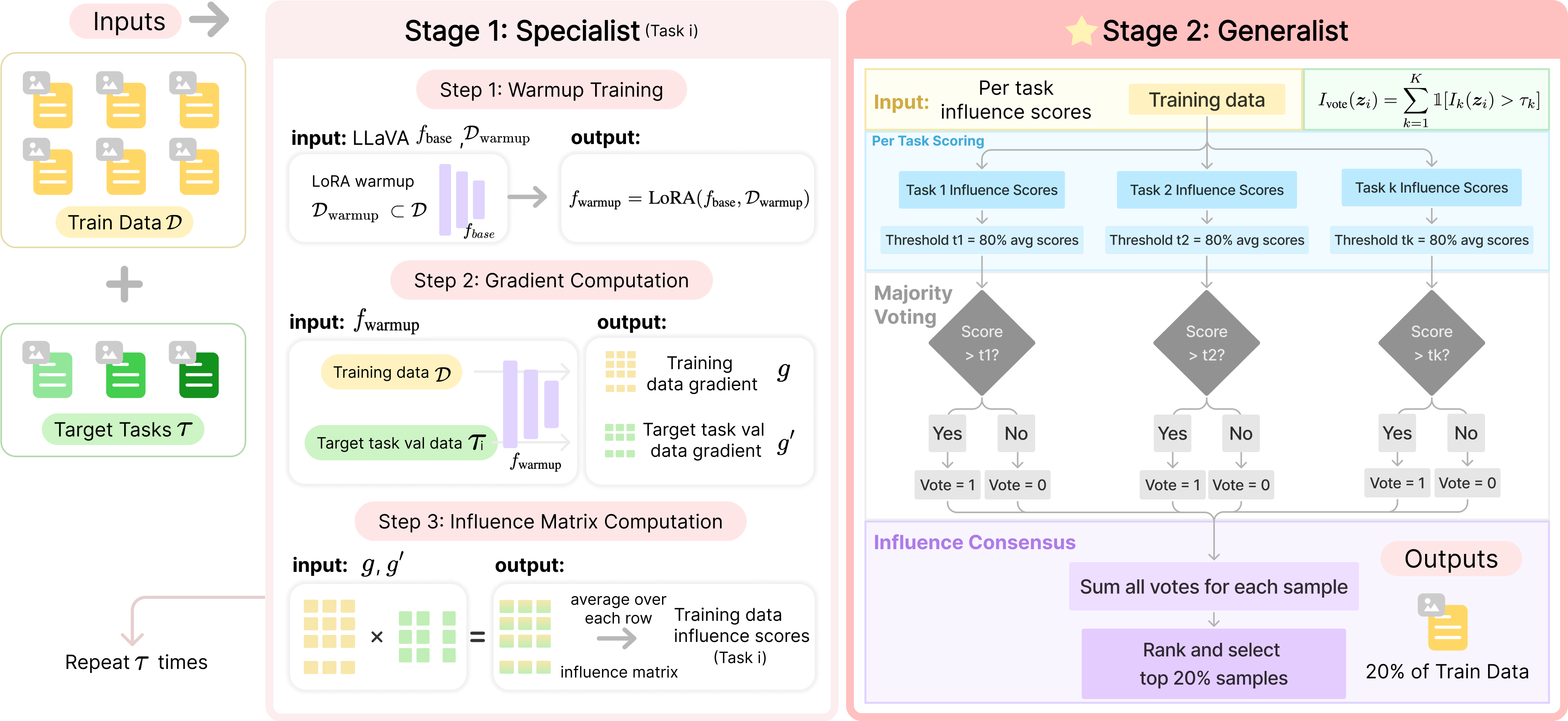
Figure 2: ICONS. The Specialist stage (left) processes each task individually through three steps: (1) warmup training on a small subset of data, (2) gradient computation for both training and target task validation data, and (3) influence matrix computation to generate per-task influence scores. This process is repeated for each target task. The Generalist stage (right) performs Influence Consensus to aggregate information across tasks, where samples scoring above the $80^{\text{th}}$ percentile threshold for each task receive a vote. The final selection is made by summing votes across tasks and selecting the top 20% most influential samples, creating a compact yet highly effective training dataset that performs well across all tasks.

2.1 Problem Formulation

Given a large-scale visual instruction tuning dataset $\mathcal{D}=\{({\bm{x}}_{i},{\bm{I}}_{i},{\bm{y}}_{i})\}_{i=1}^{N}$ containing $N$ samples, where each data point ${\bm{z}}_{i}=({\bm{x}}_{i},{\bm{I}}_{i},{\bm{y}}_{i})$ includes natural language instruction ${\bm{x}}_{i}$ and an image ${\bm{I}}_{i}$, with corresponding target response ${\bm{y}}_{i}$, and given access to validation data $\mathcal{V}_{k}$ for each downstream task $T_{k}\in\mathcal{T}=\{T_{1},...,T_{K}\}$, our goal is to select a compact subset $\mathcal{S}\subset\mathcal{D}$ of size $M\ll N$ that maximizes model performance across multiple downstream tasks:

$$\mathcal{S}^{*}=\operatorname*{arg\,max}_{\mathcal{S}\subset\mathcal{D},|\mathcal{S}|=m}\sum_{k=1}^{K}\text{Rel}(f_{\mathcal{S}},T_{k}),$$ (1)

$$\text{Rel}(f_{\mathcal{S}},T_{k})=\frac{\text{Score}(f_{\mathcal{S}},T_{k})}{\text{Score}(f_{\mathcal{D}},T_{k})},$$ (2)

where $f_{\mathcal{S}}$ and $f_{\mathcal{D}}$ denote models trained on subset $\mathcal{S}$ and full dataset $\mathcal{D}$, respectively. $\text{Score}(f,T_{k})$ is the task-specific evaluation score achieved by model $f$ on task $T_{k}$. We define the average relative performance across all tasks as Rel. = $\sum_{k=1}^{K}\text{Rel}(f_{\mathcal{S}},T_{k})/K$. Rel. quantifies the subset-trained model’s performance relative to that of the model trained on the entire dataset, with values close to 1 indicating that the subset maintains the performance of full training [18]. Our objective is to find a subset where Rel. $\approx 1$, i.e., the model trained on the selected subset achieves performance comparable to using the full dataset across all tasks.

2.2 Preliminaries

Building on our problem formulation in §2.1, we formalize how to estimate the influence of training samples on downstream task performance. Specifically, since our goal is to maximize $\text{Rel}(f_{\mathcal{S}},T_{k})$ across tasks as defined in Eqn. 2, we need an efficient way to estimate how each training sample contributes to the $\text{Score}(f_{\mathcal{S}},T_{k})$ term in the numerator. Following [34, 42], we estimate how individual training samples $z_{i}\in\mathcal{D}$ affect validation loss by measuring their gradient alignment with reducing validation loss on $\mathcal{V}_{k}$, which directly impacts task-specific evaluation scores. Denote a training data point as ${\bm{z}}$ and a validation data point as ${\bm{z}}^{\prime}$ from validation set $\mathcal{V}_{k}$ for task $T_{k}$ When training with SGD and batch size 1, using data point ${\bm{z}}$ at timestep $t$ leads to a model update ${\bm{\theta}}_{t+1}={\bm{\theta}}_{t}-\eta_{t}\nabla\ell({\bm{z}};{\bm{\theta}}_{t})$, where $\eta_{t}$ is the learning rate. To reduce the computational cost, we use the first-order Taylor expansion to estimate the loss on a given validation data point ${\bm{z}}^{\prime}$ at time step $t+1$ as:

$$\ell({\bm{z}}^{\prime};{\bm{\theta}}_{t+1})\approx\ell({\bm{z}}^{\prime};{\bm{\theta}}_{t})+\langle\nabla\ell({\bm{z}}^{\prime};{\bm{\theta}}_{t}),{\bm{\theta}}_{t+1}-{\bm{\theta}}_{t}\rangle.$$

The influence of a training data point ${\bm{z}}$ on a validation data point ${\bm{z}}^{\prime}$ is:

$$\mathcal{I}_{t}({\bm{z}}\rightarrow{\bm{z}}^{\prime}) =\ell({\bm{z}}^{\prime};{\bm{\theta}}_{t+1})-\ell({\bm{z}}^{\prime};{\bm{\theta}}_{t})$$

$$\approx-\eta_{t}\langle\nabla\ell({\bm{z}}^{\prime};{\bm{\theta}}_{t}),\nabla\ell({\bm{z}};{\bm{\theta}}_{t})\rangle,$$

which we refer to as an influence score. For our case of visual instruction tuning [23] which uses single-epoch training, the influence score is:

$$\mathcal{I}_{\text{single}}({\bm{z}}\rightarrow{\bm{z}}^{\prime})=\eta\langle\nabla\ell({\bm{z}}^{\prime};{\bm{\theta}}_{t}),\nabla\ell({\bm{z}};{\bm{\theta}}_{t})\rangle,$$

where $\eta$ is the learning rate used during training. This can be generalized to multi-epoch training by accumulating the influence scores over all $n$ epochs:

$$\mathcal{I}_{\text{total}}({\bm{z}}\rightarrow{\bm{z}}^{\prime})=\sum_{i=1}^{n}\eta_{i}\langle\nabla\ell({\bm{z}}^{\prime};{\bm{\theta}}_{i}),\nabla\ell({\bm{z}};{\bm{\theta}}_{i})\rangle,$$

where $\eta_{i}$ is the learning rate used during the $i$th epoch. The gradient-based selection approach selects training samples $\{{\bm{z}}\}$ that maximize the gradient inner product $\langle\nabla\ell({\bm{z}}^{\prime};{\bm{\theta}}_{t}),\nabla\ell({\bm{z}};{\bm{\theta}}_{t})\rangle$ through a greedy, first-order approximation, which leads to larger reductions in validation loss for point ${\bm{z}}^{\prime}$. While this approach omits second-order terms compared to influence functions [17], it provides an efficient approximation for ranking the impact of training samples [11, 42].

2.3 Specialist: Individual Task Influence Ranking

To rank the influence of training data for each target task, we compute the influence score of each training data point on a validation set that represents the target task distribution. Following LESS [42], the process involves three steps: (1) training the model on 5% randomly selected data as a lightweight warm-up phase to initialize visual instruction-following capabilities, (2) computing gradients for training and validation data and compressing the gradients via random projection, and (3) computing the influence score to quantify the impact of each training data on validation set.

Step 1: Warm-up Training.  Following LESS [42], we first perform a brief warmup phase using Low-Rank Adaptation (LoRA) [12] on a small random subset $\mathcal{D}_{\mathrm{warmup}}\subset\mathcal{D}$ (5% of the training data): $f_{\text{warmup}}=\text{LoRA}(f_{\text{base}},\mathcal{D}_{\text{warmup}})$. This warmup phase allows the model to develop basic instruction-following capabilities.

Step 2: Gradient Computation.  For each training data ${\bm{z}}_{i}\in\mathcal{D}$ and validation data ${\bm{z}}^{\prime}_{j}\in\mathcal{D}_{\text{val}}^{k}$ from $\mathcal{T}_{k}$, we compute their gradients with respect to $f_{\text{warmup}}$ parameters $\theta_{w}$:

$$g_{i}=\nabla_{\theta_{w}}\mathcal{L}(f_{\text{warmup}}({\bm{z}}_{i}),{\bm{y}}_{i}),\quad g^{\prime}_{j}=\nabla_{\theta_{w}}\mathcal{L}(f_{\text{warmup}}({\bm{z}}^{\prime}_{j}),{\bm{y}}^{\prime}_{j})$$

where $y_{i}$ and $y^{\prime}_{j}$ are the targets for $z_{i}$ and $z^{\prime}_{j}$, respectively. In order to reduce computational and storage overhead, we apply random projection to the gradient feature: $\tilde{g}_{i}=Rg_{i}$ and $\tilde{g}^{\prime}_{j}=R^{\prime}g^{\prime}_{j}$, where $R,R^{\prime}\in\mathbb{R}^{d^{\prime}\times d}$ is a random projection matrix with $d^{\prime}\ll d$ that preserves inner products with high probability [14]. We further normalize the projected gradient features, $\tilde{g}_{i}=\frac{\tilde{g}_{i}}{\|\tilde{g}_{i}\|_{2}},\tilde{g}^{\prime}_{j}=\frac{\tilde{g}^{\prime}_{j}}{\|\tilde{g}^{\prime}_{j}\|_{2}}$ to prevent bias from sequence length differences [42].

Step 3: Influence Matrix Computation.  We compute the influence matrix $I\in\mathbb{R}^{|\mathcal{D}|\times|\mathcal{D}_{\text{val}}^{k}|}$ where each entry $I_{ij}=\langle\tilde{g}_{i},\tilde{g}^{\prime}_{j}\rangle$ is the influence of training data ${\bm{z}}_{i}$ on validation data ${\bm{z}}^{\prime}_{j}$, and the average influence of training data ${\bm{z}}_{i}$ on the target task $k$ is then computed as:

$$\bar{I}_{k}({\bm{z}}_{i})=\frac{1}{|\mathcal{D}_{\text{val}}^{k}|}\sum_{j=1}^{|\mathcal{D}_{\text{val}}^{k}|}I_{ij}.$$ (3)

This influence estimation process provides a task-specific ranking for the training set $\mathcal{D}$ with respect to task $\mathcal{T}_{k}$, where a higher influence score $\bar{I}_{i}$ suggests a higher influence for the target task. However, recall that our ultimate goal is to select a compact subset $\mathcal{S}\subset\mathcal{D}$ of size $M\ll N$ that maximizes $\sum_{k=1}^{K}\text{Rel}(f_{\mathcal{S}},T_{k})/K$ across all tasks. We address this disconnection between task-specific rankings and overall dataset optimization by proposing a voting-based generalist approach; this approach aggregates influence scores for each target task to identify the most broadly impactful training data.

2.4 Generalist: Cross-Task Influence Consensus

Our consensus-based voting strategy identifies training samples that consistently show a high influence score across various tasks. For each task $k$, we set a task-specific threshold $\tau_{k}$ at the $((1-p)\times 100)$-th percentile of the influence score distribution within that task, where $p$ represents the proportion of top samples to consider ($p=0.2$ in our main experiments). A sample ${\bm{z}}_{i}$ is considered important for task $k$ if its influence score $I_{k}({\bm{z}}_{i})\geq\tau_{k}$. Formally, we define the voting-based influence score for sample $z_{i}$ on task $k$ as:

$$I_{\text{vote}}({\bm{z}}_{i})=\sum_{k=1}^{K}\mathbbm{1}[I_{k}({\bm{z}}_{i})\geq\tau_{k}],$$ (4)

where $\mathbbm{1}[\cdot]$ denotes the indicator function, and $I_{k}({\bm{z}}_{i})$ represents the influence score of sample ${\bm{z}}_{i}$ for task $k$. The final score for each sample is the total number of votes it receives across all tasks, ranging from 0 (indicating no importance for any task) to $K$ (indicating consistent importance for all tasks). Influence Consensus identifies a unique subset of samples that are consistently influential across multiple tasks, rather than those that might be highly influential in only a few tasks. After computing the aggregated influence scores, we rank the training samples and select the top $p\%$ as final subset for model training.

While directly combining validation data from all target tasks and computing a single influence matrix (Direct-merge Selection, §3.5) might seem intuitive, we adopt this consensus-based approach for three reasons. First, specialist selection provides a practical performance upper bound, as the performance achieved by selecting the top $p$% of data specifically for a single task represents the theoretical maximum achievable with that data budget, serving as a critical baseline for evaluating generalist selection trade-offs (§3.5). Second, this approach is scalable and naturally supports continual learning scenarios, as influence matrices for new tasks or benchmarks can be computed independently without recomputing training gradients, thereby reducing computational costs. Third, computing influence matrices independently for different tasks give us better understanding of cross-task influence dynamics. Our analysis (§3.3) reveals that the influence ranking of training data vary significantly across different tasks, with highly influential samples for one task often showing limited impact on others. This further provides insights to design more effective consensus mechanisms for generalist selection while maintaining computational tractability.

Method	VQAv2	GQA	VizWiz	SQA-I	TextVQA	POPE	MME	MMBench		LLaVA-W	Rel. (%)
								en	cn	Bench
Full	79.1	63.0	47.8	68.4	58.2	86.4	1476.9	66.1	58.9	67.9	100
Random	75.7	58.9	44.3	68.5	55.3	84.7	1483.0	62.2	54.8	65.0	95.8
CLIP-Score [35]	73.4	51.4	43.0	65.0	54.7	85.3	1331.6	55.2	52.0	66.2	91.2
EL2N [33]	76.2	58.7	43.7	65.5	53.0	84.3	1439.5	53.2	47.4	64.9	92.0
Perplexity [28]	75.8	57.0	47.8	65.1	52.8	82.6	1341.4	52.0	45.8	68.3	91.6
SemDeDup [1]	74.2	54.5	46.9	65.8	55.5	84.7	1376.9	52.2	48.5	70.0	92.6
D2-Pruning [26]	73.0	58.4	41.9	69.3	51.8	85.7	1391.2	65.7	57.6	63.9	94.8
Self-Sup [38]	74.9	59.5	46.0	67.8	49.3	83.5	1335.9	61.4	53.8	63.3	93.4
Self-Filter [5]	73.7	58.3	53.2	61.4	52.9	83.8	1306.2	48.8	45.3	64.9	90.9
COINCIDE [18]	76.5	59.8	46.8	69.2	55.6	86.1	1495.6	63.1	54.5	67.3	97.4
ICONS (ours)	76.3	60.7	50.1	70.8	55.6	87.5	1485.7	63.1	55.8	66.1	98.6

Table 1: Baseline Comparisons. Performance comparison of different data selection approaches when trained on 20% of the LLaVA-665K dataset. Models are evaluated across diverse multimodal benchmarks, with tasks ranging from visual question answering (VQAv2, GQA) to multilingual understanding (MMBench). The best and second best results for each benchmark are shown in bold and underlined, respectively. Our method ICONS achieves the highest overall relative performance (98.6%), consistently outperforming existing approaches including COINCIDE (97.4%) and D2-Pruning (94.8%), while methods like EL2N, Perplexity, and CLIP-Score show limited effectiveness with relative performance around 91-92%.

3 Experiments

In this section, we first discuss our experiment setup and evaluation benchmarks (§3.1). Then we compare it with the latest state-of-the-art methods (§3.2). Next, we provide detailed analysis of our method’s behavior and effectiveness across different dimensions (§3.3). We further evaluate the transferability of our selection approach across both unseen tasks and model architectures (§3.4). Finally, we conduct ablation studies to understand the contribution (§3.5).

3.1 Evaluation Test-Bed

Dataset & Model.  We evaluate ICONS on visual instruction tuning dataset LLaVA-665K [22]. We use LLaVA-v1.5-7b-lora model [22] with a default size of 7B parameters unless otherwise specified. In all experiments, we train the models for one epoch following the official finetuning hyperparameters, which reduces computational overhead while maintaining selection quality.

Target Tasks.  We evaluate the effectiveness of ICONS with a wide range of multimodal benchmarks (Tab. 2) that test different capabilities of vision-language models. The benchmarks include: 1) Multiple-choice understanding: MMBench [47] and MME [7], which assess the model’s ability to select correct answers from given options; 2) Visual question answering: VQAv2 [9], GQA [13], and VizWiz [10], which test basic visual reasoning; 3) Text understanding in images: TextVQA [37], which evaluates OCR capabilities; 4) Scientific reasoning: ScienceQA [25], which tests knowledge-grounded question answering; 5) Open-ended generation: LLaVA-W Bench [23], which evaluate free-form response generation; 6) Factual consistency: POPE [21], which measures hallucination.

	MME	POPE	SQA-I	MMBench
				en	cn
$|\mathcal{D}_{\text{val}}|$	986	500	424	1,164	1,164
$|\mathcal{D}_{\text{test}}|$	2,374	8,910	4,241	1,784	1,784
Task Type	Y/N	Y/N	MCQ	MCQ	MCQ
	VQAv2	GQA	VizWiz	TextVQA	LLaVA-W
$|\mathcal{D}_{\text{val}}|$	1,000	398	8,000	84	84
$|\mathcal{D}_{\text{test}}|$	36,807	12,578	8,000	5,000	84
Task Type	VQA	VQA	VQA	VQA	VQA

Table 2: Statistics of Target Tasks. Our target tasks include diverse benchmarks and answer formats, covering different vision-language capabilities. Task types include Multiple-Choice Questions (MCQ), Visual Question Answering (VQA), and Yes/No Questions (Y/N).

3.2 Comparisons with Baselines

We compare our ICONS against several baseline approaches, including random selection. We evaluate CLIP-Score [35] for measuring image-text alignment, EL2N [33] based on embedding L2 norms, and Perplexity [28] using language model scores. We also compare against SemDeDup [1] for semantic deduplication and D2-Pruning [26] for distribution-aware pruning. Additional baselines include Self-Sup [38] leveraging self-supervised signals, while Self-Filter [5] and COINCIDE [18] are the approaches specifically designed for vision-language data selection. All methods are evaluated using a 20% sampling ratio of the original dataset, with results presented in Tab. 1. We reference the baseline results from COINCIDE [18].

We compare our ICONS against existing data selection approaches in Tab. 1. Our method achieves the best overall performance with 98.6% Rel., outperforming all baselines with LLaVA-ICONS-133K, 20% of the training data. Remarkably, we achieve comparable or better performance than training with the entire LLaVA-665K on several tasks: SQA-I (70.8 vs. 68.4), MME (1485.7 vs. 1476.9), VizWiz (50.1 vs. 47.8) and POPE (87.5 vs. 86.4). Among the baselines, COINCIDE achieves strong performance (97.4% Rel.), though it falls short of ICONS on key tasks. Other methods like EL2N, Perplexity, SemDeDup are less effective, with relative scores around 91-92%, showing limitations in preserving performance.

Task	Full	Specialist	Generalist	Delta (%)
VQAv2 [9]	79.1	77.1	76.3	1.04
GQA [13]	63.0	61.1	60.7	0.65
VizWiz [10]	47.8	53.1	50.1	5.65
SQA-I [25]	68.4	69.8	70.8	-1.43
TextVQA [37]	58.2	55.7	55.6	0.18
POPE [21]	86.4	86.6	87.5	-1.04
MME [7]	1476.9	1506.1	1485.7	1.35
MMBench (en) [47]	66.1	66.0	63.1	4.34
MMBench (cn) [47]	58.9	56.4	55.8	1.06
LLaVA-W Bench [23]	67.9	67.1	66.1	1.49

Table 3: Single-task Selection (Specialist) vs. Consensus-aware Multi-task Selection (Generalist). The single-task data selection approach selects 20% of data per task, while our consensus-aware multi-task data selection approach selects a total of 20% data across all tasks. The Delta (%) column represents the relative drop in performance from specialist to generalist.

Figure 3: Data Overlap between Specialists and Generalist Selection. It shows varying degrees of overlap, ranging from 3.27% (VQAv2 [9]) to 24.21% (LLAVA-W Bench [23]).

Figure 4: Performance Comparison at Different Selection Ratios. Here we show the average relative performance comparisons of various data selection methods at different selection ratios. Our ICONS consistently outperforms all baseline approaches across different selection ratios, achieving 99.2% relative performance with 40% of the data, and remarkably exceeding 102% at 60% selection ratio. This shows that our selected subset is not only more efficient but can be even more effective than the full dataset for model training.

3.3 Analysis

From Specialist to Generalist.  In order to understand the effectiveness of the intermediate task-specific influence matrices we obtained from the specialist stage, we further conduct experiments on selecting 20% of data for individual tasks. As shown in Tab. 3, using 20% task-specific data, it achieves comparable or even superior performance to full data training in several cases (e.g., MME from 1476.9 to 1506.1 and SQA-I from 68.4 to 69.8). Then, through our influence consensus mechanism in the generalist stage, we identify consistently influential cross-tasks samples and select a 20% subset. This generalist approach maintains remarkably strong performance, with an average drop of 1.33% across most tasks compared to specialist baselines.

As visualized in Fig. 3, the overlap between specialist and generalist selections varies significantly across tasks, ranging from minimal overlap in simpler tasks like VQAv2 [9] (3.27%) and VizWiz [10] (3.28%) to substantial agreement in more complex tasks like LLAVA-W Bench [23] (24.21%). Notably, some tasks even show performance improvements under the generalist selection, such as SQA-I [25] (improving by 1.43%) and POPE [21] (improving by 1.04%). This empirically validates our consensus-based approach: by first understanding task-specific influence patterns and then building consensus across tasks, we can effectively identify a compact, universal training set that maintains strong performance across diverse vision-language tasks while significantly reducing the required training data.

Different Selection Ratio.  We evaluate our ICONS against baseline methods across different selection ratios, ranging from 5% to 60% of the training data. As shown in Fig. 4, our results reveal several key patterns: First, ICONS shows particularly strong performance in the low-selection regime (5-20%), where identifying the most influential samples is crucial. Another notable observation is that as the selection ratio increases, the performance gap between different methods gradually narrows. This convergence pattern is expected, as larger sample sizes naturally capture more of the dataset’s diversity and information. Despite this convergence trend, ICONS consistently maintains its performance edge across all selection ratios, and remarkably reaching above 100% at 60% selection ratio. One hypothesis is that ICONS can also effectively filter out potentially harmful or noisy training samples that might negatively impact model training, thereby surpassing the full training performance.

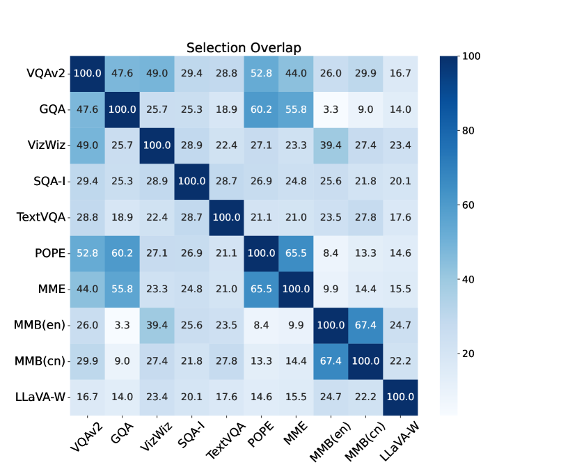
(a) Pairwise Overlap Heatmap between Specialist Benchmarks. The values are the percentage of selected overlapping samples across different benchmarks, with high overlap seen between POPE and GQA (60.2%) and between VQAv2 and VizWiz (49.0%). Lower overlap, such as 3.3% between MMBench(en) and GQA, shows more distinct selected sample sets.

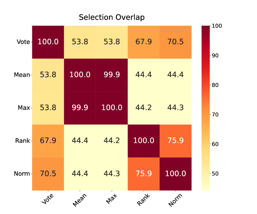
(b) Pairwise Overlap Heatmap between Different Aggregation Approaches. The values are the percentage of overlapping selected samples between each pair of aggregation approaches. Our Vote-based influence consensus approach shows moderate overlap (53.8%-70.5%) with other methods, while Mean and Max selections are highly correlated (99.9%).

Figure 5: Pairwise Overlap Heatmaps between Different Aggregation Approaches and Benchmarks. (a) compares the overlap between different specialist benchmarks, while (b) shows overlap between various aggregation methods.

Divergent Cross-Task Influence Patterns.  As shown in Fig. 5(a), the pairwise overlap heatmap reveals significant variation in training data influence rankings across different tasks. High overlap, such as between VQAv2 and VizWiz (49.0%) or POPE and GQA (60.2%), suggests that certain samples are beneficial across similar tasks. However, low overlap, like the 3.3% between MMBench (en) and GQA, highlights that highly influential samples for one task may have limited impact on others. Even closely related tasks, such as MMBench in different languages (English and Chinese), share 67.4% of influential samples. These findings empirically demonstrate significant overlap in influential samples across tasks, motivating the use of influence consensus for effective multi-task data selection.

3.4 Transferability

We evaluate the transferability of our data selection approach across two dimensions: unseen-task generalization and cross-architecture-scale generalization. Unseen-task Generalization.  LLaVA-ICONS-133K demonstrates exceptional generalization on entirely unseen benchmarks that were not considered during our data selection process. As shown in Tab. 4, we test across a diverse spectrum of tasks including MMVet [45], NaturalBench [19], AI2D [16], ChartQA [29], DocVQA [30], InfoVQA [31], RealWorldQA [41] and CMMMU [46]. LLaVA-ICONS-133K achieves 95.5-113.9% (Rel.) compared to full dataset training. Notably, we observe improvements on InfoVQA (103.8%), NaturalBench (105.5%), RealWorldQA (104.4%), and CMMMU (113.9%), suggesting that, in some cases, training on LLaVA-ICONS-133K may even outperform training on the full dataset, despite these tasks not being included in the selection process. Importantly, LLaVA-ICONS-133K significantly outperforms random selection across all benchmarks - for example, improving performance on ChartQA (17.1 vs. 15.1), MMVet (29.7 vs. 27.6), CMMMU (25.2 vs. 21.9) and NaturalBench (12.8 vs. 11.1). This consistent improvement over random selection further validates the effectiveness of ICONS. This suggests that our selection approach successfully captures fundamental visual-language understanding capabilities that transfer well across different task formats and domains, and consistently outperforms random selection by a significant margin.

	AI2D	ChartQA	DocVQA	InfoVQA	MMVet	Naturalbench	RealworldQA	CMMMU	Rel. (%)
Full	55.4	17.5	28.9	26.5	31.1	12.4	52.4	22.1	100.0
Random	50.2	15.1	25.2	24.3	27.6	11.1	49.8	21.9	91.6
LLaVA-ICONS-133K	53.9	17.1	27.9	27.5	29.7	12.8	55.0	25.2	98.7
Per-task Rel. (%)	97.3	97.7	96.5	103.8	95.5	103.2	104.4	114.0	-

Table 4: Unseen-Task Generalization. Performance comparison on unseen benchmarks when trained on the selected subset. The relative performance ratios show that our selection approach successfully captures fundamental visual-language understanding capabilities that transfer well across different task formats and domains. Notably, we observe improvements on InfoVQA [31] (103.8%), MMVet [45] (95.5%), NaturalBench [19] (103.2%), RealWorldQA [41] (104.4%), and CMMMU [46] (114.0%), suggesting that in some cases, training on our LLaVA-ICONS-133K may even outperform using the full dataset.

Cross-Architecture-Scale Generalization.  We further conduct experiments on cross architecture scale generalization to evaluate the transferability of our selected data across different model scales. While our subset was initially selected using LLaVA-1.5-7B as the base model, we investigate whether these same examples remain effective for training larger architectures like LLaVA-1.5-13B. This tests whether our selection criteria identify universally valuable training examples rather than model-specific patterns. Our results in Tab. 5 show cross architecture scale generalization, with the 7B-selected achieving 98.1% relative performance, suggesting that our selected subset captures fundamental visual-language understanding capabilities that scale effectively across model sizes.

	VQAv2	GQA	Vizwiz	SQA-I	TextVQA	POPE	MME	MMBench	MMBench(cn)	LLAVA-W	Rel. (%)
Full	80.0	63.3	58.9	71.2	60.2	86.7	1541.7	68.5	61.5	69.5	100.0
Random	77.3	60.7	57.6	69.1	56.8	82.9	1517.2	63.2	56.3	67.5	95.7
7B-selected	78.8	60.4	57.4	70.4	58.3	84.3	1527.5	64.9	59.7	68.2	97.3
13B-selected	78.9	61.2	57.5	71.3	58.4	85.9	1535.2	66.1	59.8	68.8	98.1

Table 5: Cross-Architecture-Scale Generalization. Our LLaVA-ICONS-133K selected via LLaVA-v1.5-7b-lora (7B-selected) shows strong cross-architecture transferability, achieving competitive performance when trained with data selected via LLaVA-v1.5-13b-lora (13B-selected). Specifically, while the 7B-selected achieves 97.3% relative performance, the 13B-selected model reaches 98.1%, showing that our selected subset’s effectiveness scales well to larger architectures. Both significantly outperform random selection (95.7%), with the 13B-selected option showing particular strength in complex reasoning tasks like MMBench and POPE. This consistency across model scales highlights that our data selection approach captures fundamental visual-language understanding patterns that generalize well across different model architecture scales.

3.5 Ablation Studies

Different Aggregation Approaches.  To understand how different methods of combining task-specific influence scores affect the performance, we compare our majority voting approach (Vote) with four aggregation approaches: (1) Mean, which averages scores across tasks, (2) Max, which selects the highest score per sample, (3) Rank, which averages the relative ranking of samples within each task, (4) Norm, which normalize the scores before averaging:

$$I_{\text{mean}}({\bm{z}}_{i})=\frac{1}{K}\sum_{k=1}^{K}I_{k}({\bm{z}}_{i})\qquad I_{\text{norm}}({\bm{z}}_{i})=\frac{1}{K}\sum_{k=1}^{K}\frac{I_{k}({\bm{z}}_{i})-\mu_{k}}{\sigma_{k}}$$

$$I_{\text{max}}({\bm{z}}_{i})=\max_{k=1,\ldots,K}I_{k}({\bm{z}}_{i})\qquad I_{\text{rank}}({\bm{z}}_{i})=\frac{1}{K}\sum_{k=1}^{K}\text{rank}(I_{k}({\bm{z}}_{i}))$$

Results in Tab. 6 show that our Vote consistently outperforms alternatives across most tasks, achieving the highest overall relative performance (Rel.) of 98.6%. While methods like Rank perform well for MME (1490.0 vs. 1485.7 with Norm), they underperform overall. To better understand the relationships between these aggregation approaches, we visualize their pairwise selection overlap in Fig. 5(b). Specifically, the Mean and Max approaches show an extremely high overlap of 99.9%, suggesting they tend to select very similar influential samples. In contrast, our Vote-based approach exhibits a more moderate overlap with other methods, ranging from 53.8% to 70.5%, potentially those that are influential across a broader variety of tasks rather than overfitting to specific tasks.

Task	Mean	Max	Rank	Norm	Vote (ours)
VQAv2 [9]	75.7	75.2	74.9	75.1	76.3
GQA [13]	59.6	59.8	58.6	60.1	60.7
VizWiz [10]	47.9	48.1	40.5	46.4	50.1
SQA-I [25]	65.5	66.2	69.8	69.8	70.8
TextVQA [37]	55.5	55.5	55.2	54.5	55.6
POPE [21]	86.0	85.5	85.6	85.6	87.5
MME [7]	1422.1	1470.7	1490.0	1482.6	1485.7
MMBench (en) [47]	59.0	58.3	59.0	58.9	63.1
MMBench (cn) [47]	51.0	51.8	50.8	52.5	55.8
LLaVA-W Bench [23]	66.2	66.2	66.4	66.3	66.1
Rel.(%)	96.4	96.1	95.9	96.8	98.6

Table 6: Comparison of Different Aggregation Approaches. Performance comparison of different methods for combining task-specific influence scores, using 20% of training data. All scores are relative to full dataset training.

Task	Full	Direct	Consensus	Delta (%)
		merge	aware (ours)
VQAv2 [9]	79.1	76.1	76.3	0.26
GQA [13]	63.0	59.4	60.7	2.19
VizWiz [10]	47.8	46.1	50.1	8.67
SQA-I [25]	68.4	68.7	70.8	3.06
TextVQA [37]	58.2	54.1	55.6	2.77
POPE [21]	86.4	85.1	87.5	2.82
MME [7]	1476.9	1419.2	1485.7	4.69
MMBench (en) [47]	66.1	61.9	63.1	1.94
MMBench (cn) [47]	58.9	50.3	55.8	10.94
LLaVA-W Bench [23]	67.9	65.2	66.1	1.38
Rel. (%)	100	94.7	98.6	-

Table 7: Comparison of Consensus-aware vs. Direct-merge Selection. Performance comparison across different benchmarks using 20% of training data. Direct-merge computes influence directly on combined validation sets, while consensus-aware refers to our specialist-to-generalist approach. The Delta (%) column represents the relative improvement from Direct-merge to Consensus-aware. Consensus-aware outperforms Direct-merge across all benchmarks, while Direct-merge notably underperforms even the random baseline.

Consensus-aware Selection vs. Direct-merge Selection.  To validate our choice of a consensus-aware approach (first computing task-specific influence matrices and then aggregating results) versus a direct-merge approach (directly computing influence using a combined validation set), we compare the performance of both approaches. In the direct-merge approach, we combine validation sets from all tasks into a single pool, denoted as $\{{\bm{z}}^{\prime}\}_{\mathrm{merged}}$, and compute influence scores directly against this combined set: $\mathcal{I}_{\text{direct}}({\bm{z}}\rightarrow\{{\bm{z}}^{\prime}\}_{\mathrm{merged}})$. As described in Tab. 7, our consensus-aware approach consistently outperforms direct-merge selection across all benchmarks, with the largest gains observed on complex tasks like MME [7].

A potential reason could be the direct-merge approach does not account for the different vision-language task difficulties or validation set sizes across the target tasks. By pooling all validation examples, it effectively treats each validation data from all tasks equally, which can lead to the influence scores being dominated by tasks with more samples or with higher influence scores on average. The task-aware voting-based influence consensus mechanism of our direct-merge approach are more robust to these issues. Additionally, our approach is more scalable, as it avoids computing a single, large influence matrix across validation data from all target tasks. Adding new tasks only requires computing influence scores for those specific tasks and updating the voting mechanism, while direct-merge selection would need to recompute the entire large influence matrix which makes it less practical.

4 Related Work

Visual Instruction Tuning.

Multimodal large language models (MLLMs), e.g., Flamingo [2], LLaVA [23], BLIP2 [20], and Cambrian [39], enhance the capabilities of large language models (LLMs) on various multimodal tasks. A key component in advancing MLLMs is visual instruction tuning [23], a training process that enables these models to interpret and follow instructions within a vision-language context, transforming them into versatile multimodal assistants. This tuning process not only improves the models’ instruction-following abilities but also aligns their outputs more closely with user expectations, thus enhancing their utility in practical applications [23].

Data Selection.

Data selection methods can be categorized based on the types of information they utilize for selection. Representation-based approaches [1, 18] leverage neural embeddings to capture data representations. Loss trajectory-based methods [32] prioritize data points that contribute most significantly to reducing generalization error over training. Gradient-based techniques [33, 42, 6] select data based on gradient information. Recent work has explored various approaches to select optimal visual instruction tuning datasets. Concurrent work TIVE [24] employs gradient-based selection to identify representative instances. TIVE assumes that the number of specialist data should be proportional to task difficulty and thus samples specialist data based on an estimation of task difficulty. Our method does not rely on this assumption – we directly select samples that benefit the greatest number of tasks. COINCIDE [18] clusters data based on representations associated with concept-skill compositions. Our work follows targeted instruction tuning selection approach LESS [42] to utilize gradient information to calculate the specialist influence (i.e., the influence on a specific task) and extends it to general scenarios by aggregating information from various tasks and selecting data for multiple downstream tasks via majority voting.

5 Conclusion

In this work, we introduce ICONS, a simple yet effective influence consensus-based approach for visual instruction tuning data selection. Our two-stage specialist-to-generalist method, first computes task-specific influence matrices and then select a subset by prioritizing universally influential samples through a cross-task voting mechanism. Through extensive experiments, we show that ICONS achieving 98.6% of full dataset performance using only 20% of the data and it consistently outperform baseline methods across different selection ratios. Additionally, we release LLaVA-ICONS-133K, a 20% subset of LLaVA-665K dataset, that not only maintains strong performance across diverse vision-language tasks but also shows transferability to unseen tasks. We hope our work inspires further exploration into data-efficient methods for vision-language models across diverse applications.

Limitations.  Our approach primarily faces one practical limitation: computing gradients for large training datasets is computationally expensive (§B.2). This computational overhead could potentially constrain the method’s applicability when working with extremely large-scale datasets. To support broader research community, we release our LLaVA-ICONS-133K dataset to help research iteration and model development under resource-constrained settings.

Acknowledgments.  This material is based upon work supported by the National Science Foundation under Grant No. 2107048 and No.2112562. Any opinions, findings, and conclusions, or recommendations expressed in this material are those of the author(s) and do not necessarily reflect the views of the National Science Foundation. This work is also supported by the Singapore National Research Foundation and the National AI Group in the Singapore Ministry of Digital Development and Information under the AI Visiting Professorship Programme (award number AIVP-2024-001). We thank many people for their helpful discussion and feedback, listed in alphabetical order by last name: Allison Chen, Hamish Ivison, Carlos E. Jimenez, Polina Kirichenko, Jaewoo Lee, Tiffany Ling, Zhiqiu Lin, Shengbang Tong, Ethan Tseng, Justin Wang, Zirui Wang.

Appendix for ICONS: Influence Consensus for Vision-Language Data Selection

In this supplement, we provide additional experiment details and ablation studies (§A) and additional analysis (§B). We detail our algorithmic framework (§C) and discuss future research directions (§D). Finally, we include visualization of the selected data (§E) to better understand data samples with high influence.

Appendix A Additional Experiment Details & Ablations

Projection Dimension.  We primarily set the projection dimension to 5120, reducing features from 338.7M to 5120 dimensions. The choice of 5120 was empirically validated for its trade-off between effective capturing gradient representation and maintaining a manageable parameter space. Our LLaVA-v1.5-7b-lora architecture includes a total of 7.4B parameters, with 338.7M parameters being trainable after LoRA adaptation, accounting for approximately 4.58% of the total parameter count. We further ablate different projection dimensions (1024, 2560, 5120, and 10240), with results provided in Fig. 6.

Warm-up Ratio.  To initiate training, we use a warm-up set including 5% of the total training data. We conducted ablation studies to evaluate the impact of varying warm-up ratios (5%, 10%, 20%, and 100%) on selection performance, as shown in Fig. 7. Our experiments reveal that increasing the warm-up data size does not lead to performance improvements. Surprisingly, models trained with smaller warm-up ratios (5-20%) consistently outperform those trained with the full dataset (100%). Specifically, the 5% warm-up ratio achieves the best performance at 98.6%, while using the complete dataset results in a performance drop to 97.8%. This finding suggests that a small subset of training data is sufficient and even beneficial for model initialization, and potentially gives better signals in the early training stages.

Figure 6: Projection Dimension Ablation. We show the performance of ICONS at different projected dimensions (1024, 2560, 5120, 10240), compared to the random baseline. The performance increases with the projected dimension and reaches a plateau around dimension 5120.

Figure 7: Warm-up Ratio Ablation. The blue line represents ICONS performance across different warm-up ratios (5%, 10%, 20%, and 100%), while the red dashed line shows the random baseline performance. Results show that smaller warm-up ratios (5-20%) achieve better performance compared to using the full dataset (100%).

Appendix B Additional Analysis

B.1 Consistency Analysis

To evaluate the consistency of our approach, we conduct three independent runs of the experiment. As shown in Fig. 8, our method demonstrates high consistency across different runs, achieving 98.6$\pm$1.2% Rel., which shows a notable improvement over the random baseline, which achieves 95.8$\pm$2.7%. The lower standard deviation in our results (1.2% vs 2.7%) further indicates that our approach produces more stable and reliable outcomes compared to the random baseline.

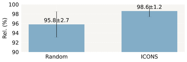
Figure 8: Rel. (%) Across Runs. We show the performance across three different runs for random selection and our ICONS. Our ICONS achieves 98.6$\pm$1.2% while the random baseline reaches 95.8$\pm$2.7%.

B.2 Computational Complexity

Computing gradient-based influence requires significant computational resources. In the specialist stage, the complexity scales with both the dataset size $|\mathcal{D}|$ and the gradient dimension $d$. This stage consists of three steps. First, the warm-up training has a complexity of $\mathcal{O}(|\mathcal{D}_{\text{warmup}}|)$. Second, the gradient computation stage has a computational complexity of $\mathcal{O}(|\mathcal{D}|+|\mathcal{D}_{\text{val}}|)$ for forward and backward passes, with storage requirements of $\mathcal{O}(|\mathcal{D}|\cdot d+|\mathcal{D}_{\text{val}}|\cdot d)$ for the gradients. Third (and finally), the influence matrix computation requires $\mathcal{O}(|\mathcal{D}|\cdot|\mathcal{D}_{\text{val}}|\cdot d^{\prime})$ compute cost, where $d^{\prime}$ is the reduced dimension after projection. The generalist stage, focusing on influence consensus across tasks, has lower computational requirements. It begins with threshold computation, requiring $\mathcal{O}(K\cdot|\mathcal{D}|\log|\mathcal{D}|)$ operations for sorting across $K$ tasks. The voting process then takes $\mathcal{O}(K\cdot|\mathcal{D}|)$ compute, followed by a final selection step with complexity $\mathcal{O}(|\mathcal{D}|\log|\mathcal{D}|)$ for sorting the aggregated votes. Storage requirements for this stage are minimal, primarily needing space for the final selected subset.

In practice, for LLaVA-665K training data, the warmup training phase requires 0.75 hours using eight L40 GPUs. We parallelize the gradient computation across 100 A6000 GPUs, taking approximately one hour and requiring 103GB of total storage for the gradients. The influence consensus stage is notably efficient, completing in less than a minute on a single L40 GPU. While these computational demands are substantial, they represent front-loaded, one-time costs that can be used across multiple target tasks and model iterations. This makes our method extendable for new tasks, as the expensive training data gradient computations only need to be performed once.

B.3 Visual Dependency Influence Ranking

Recent work [39] has shown that vision-language tasks vary in their reliance on visual information: task like MMBench [47] depends heavily on visual grounding, while others like SQA-I [25] can be handled primarily through language, showing only a 5% drop in performance when visual input is removed [39]. To take visual dependency of training data into consideration, we further explored gradient-based Visual Dependency Score (VDS). For each data point, we calculate the gradient of the model’s auto-regressive cross-entropy loss with both the original image and a Gaussian noise image $I_{\text{noise}}\sim\mathcal{N}(0,1)$, keeping the text input constant. This quantifies how much the visual component contributes to the model performance. We construct an adapted influence matrix: visual influence matrix $\mathcal{I}_{\texttt{VDS}}\in\mathbb{R}^{|\mathcal{D}|\times|\mathcal{D}_{\text{val}}|}$, which quantifies the visual influence of each training sample ${\bm{z}}_{i}$ on each validation sample ${\bm{z}}^{\prime}_{j}$ with respect to the model’s gradient alignment and visual dependency. $\mathcal{I}_{\text{VDS}}$ is computed as:

$$\mathcal{I}_{\texttt{VDS},ij}=\langle\nabla_{\theta}\mathcal{L}({\bm{z}}^{\prime}_{i}),\nabla_{\theta}\mathcal{L}({\bm{x}}_{j},I_{j})-\nabla_{\theta}\mathcal{L}({\bm{x}}_{j},I_{\text{noise}})\rangle,$$ (5)

where $\nabla_{\theta}\mathcal{L}({\bm{x}}_{j},I_{j})$ and $\nabla_{\theta}\mathcal{L}({\bm{x}}_{j},I_{\text{noise}})$ are the gradients computed with the original and Gaussian noise images, respectively. The visual influence matrix $\mathcal{I}_{\texttt{VDS}}$ provides insights into which training samples have the most influence on the validation samples from a visual perspective. This matrix can be used to further rank and select training data that are most impactful for tasks requiring strong visual grounding, ensuring that the selected subset effectively supports vision-dependent performance.

Our empirical results demonstrate that VDS-based data selection has varying effectiveness across different vision-language tasks (Tab. 8). The approach shows substantial improvements on tasks requiring strong visual understanding, such as open-ended generation (LLaVA-W Bench: +2.72%) and multiple-choice understanding (MMBench-EN: +1.90%, MMBench-CN: +0.90%). However, tasks that primarily rely on textual reasoning show decreased performance, including SQA-I (-1.84%) and TextVQA (-1.44%). These results align with and extend the findings in Cambrian [39], demonstrating that the effectiveness of VDS corresponds to a task’s visual dependency - tasks that maintain performance without visual inputs show limited or negative impact from VDS-based selection, while visually-dependent tasks benefit significantly. This pattern suggests that VDS effectively identifies training samples where visual information plays an important role in model learning.

Task	w/o VDS	w/ VDS	Delta (%)
VQAv2 [9]	76.3	75.8	-0.66
GQA [13]	60.7	60.9	+0.33
VizWiz [10]	50.1	50.3	+0.40
SQA-I [25]	70.8	69.5	-1.84
TextVQA [37]	55.6	54.8	-1.44
POPE [21]	87.5	86.8	-0.80
MME [7]	1485.7	1489.3	+0.24
MMBench (en) [47]	63.1	64.3	+1.90
MMBench (cn) [47]	55.8	56.3	+0.90
LLaVA-W Bench [23]	66.1	67.9	+2.72

Table 8: Impact of Visual Dependency Score (VDS) on Selection Performance. Performance comparison between influence calculation with and without VDS. VDS shows strongest improvements on LLaVA-W Bench (+2.72%), MMBench (en) (+1.90%), and MMBench (cn) (+0.90%), while tasks like SQA-I (-1.84%), TextVQA (-1.44%), and POPE (-0.80%) show significant performance drops.

Appendix C Algorithm Details

We provide detailed pseudocode for our two-stage ICONS framework. Stage 1 (specialist) computes task-specific influence scores through gradient-based analysis with efficient random projections. Stage 2 (generalist) implements our voting-based consensus mechanism to select samples that are influential across multiple tasks.

Algorithm 1 ICONS Stage 1: Specialist (Task-specific Influence Computation)

0: Training dataset $D=\{(x_{i},I_{i},y_{i})\}_{i=1}^{N}$, target tasks $T=\{T_{1},...,T_{K}\}$

0: Warm-up ratio $r$ (default 5%)

0: Task-specific influence scores $\{\bar{I}_{k}\}_{k=1}^{K}$

1: for each task $T_{k}\in T$ do

2:  // Step 1: Warm-up Training

3:  Sample warm-up set $D_{\text{warmup}}\subset D$ of size $r|D|$

4:  $f_{\text{warmup}}\leftarrow\text{LoRA}(f_{\text{base}},D_{\text{warmup}})$

5:  // Step 2: Gradient Computation

6:  for each training data $z_{i}\in D$ do

7:   $g_{i}\leftarrow\nabla_{\theta_{w}}L(f_{\text{warmup}}(z_{i}),y_{i})$

8:   $\tilde{g}_{i}\leftarrow\text{Normalize}(Rg_{i})$ {Random projection}

9:  end for

10:  for each validation data $z^{\prime}_{j}\in D_{\text{val}}^{k}$ do

11:   $g^{\prime}_{j}\leftarrow\nabla_{\theta_{w}}L(f_{\text{warmup}}(z^{\prime}_{j}),y^{\prime}_{j})$

12:   $\tilde{g}^{\prime}_{j}\leftarrow\text{Normalize}(Rg^{\prime}_{j})$

13:  end for

14:  // Step 3: Influence Matrix Computation

15:  for each $z_{i}\in D$, $z^{\prime}_{j}\in D_{\text{val}}^{k}$ do

16:   $I_{ij}^{k}\leftarrow\langle\tilde{g}_{i},\tilde{g}^{\prime}_{j}\rangle$

17:  end for

18:  // Compute average influence per training sample

19:  $\bar{I}_{k}(z_{i})\leftarrow\frac{1}{|D_{\text{val}}^{k}|}\sum_{j=1}^{|D_{\text{val}}^{k}|}I_{ij}^{k}$

20: end for

21: return  Task-specific influence scores $\{\bar{I}_{k}\}_{k=1}^{K}$

Algorithm 2 ICONS Stage 2: Generalist (Influence Consensus-based Data Selection)

0: Task-specific influence scores $\{\bar{I}_{k}\}_{k=1}^{K}$

0: Selection ratio $p$, number of tasks $K$

0: Selected subset $S\subset D$ of size $m\ll N$

1: // Compute voting thresholds

2: for each task $T_{k}\in T$ do

3:  $\tau_{k}\leftarrow(1-p)\text{-th percentile of }\{\bar{I}_{k}(z_{i})\}_{i=1}^{N}$

4: end for

5: // Voting process

6: for each training sample $z_{i}\in D$ do

7:  $I_{\text{vote}}(z_{i})\leftarrow 0$

8:  for each task $T_{k}\in T$ do

9:   $\text{vote}_{k}(z_{i})\leftarrow\mathbbm{1}[\bar{I}_{k}(z_{i})\geq\tau_{k}]$

10:   $I_{\text{vote}}(z_{i})\leftarrow I_{\text{vote}}(z_{i})+\text{vote}_{k}(z_{i})$

11:  end for

12: end for

13: // Select top samples based on total votes

14: $S\leftarrow\text{top-}p\text{ samples by }I_{\text{vote}}$

15: return  Selected subset $S$

Appendix D Future Work

Our work opens several promising research directions for improving vision-language data selection. While our work focuses specifically on visual instruction tuning data, our influence consensus approach can be naturally extended to other stages of MLLM training, such as alignment stage. The majority voting mechanism may under-represent tasks with unique characteristics or those in the long tail, as it prioritizes samples that broadly benefit multiple tasks to build the main knowledge pool. This can lead to limited support for specialized tasks or the reinforcement of spurious correlations spanning multiple tasks. Future work could explore weighted voting mechanisms, in which tasks are assigned weights based on their relative importance or contribution to overall model performance for more balanced data selection. Additionally, investigating more efficient gradient computation and storage methods would help scale these methods to larger datasets while maintaining strong performance across diverse vision-language tasks.

Appendix E Visualizations

We visualize the most influential top three examples across specialists (Figs. 9, 10, 11, 12, 13, 14, 15, 16, 17 and 18) and the generalist selection (Fig. 19), along with samples from their corresponding tasks. Notably, the selected high-influence examples by specialists show strong task-specific characteristics both structurally and contextually - they mirror the key attributes of their target tasks in terms of question structure, reasoning patterns, and required visual-language understanding capabilities. Furthermore, the visualization of top influential examples reveals distinct patterns in what makes training samples valuable for different vision-language tasks. VQAv2, GQA, and SQA-I specialists favor multi-turn Q&A scenarios that test both visual comprehension and contextual understanding, while TextVQA, POPE, and MME specialists emphasize text recognition, object verification, and spatial relationships respectively. MMBench-EN and MMBench-CN show consistent patterns despite language differences, focusing on clear, unambiguous scenes that translate well. The LLaVA-W Bench specialist prioritizes examples requiring detailed explanations and multi-step reasoning, and the answers are generally longer. The generalist model values diverse scenarios that combine multiple skills simultaneously. Common characteristics that make these examples particularly valuable include multi-turn interactions, clear visual elements, factual and inferential reasoning, cross-modal interaction, and the ability to test multiple capabilities within a single example. This suggests that the most effective training samples are those that combine multiple types of reasoning while maintaining clear, unambiguous ground truth that can be consistently learned across tasks.

Figure 9: VQAv2. Top-left: A sample from VQAv2 [9]. Remaining panels show top three influential samples selected using the specialist influence ranking step.

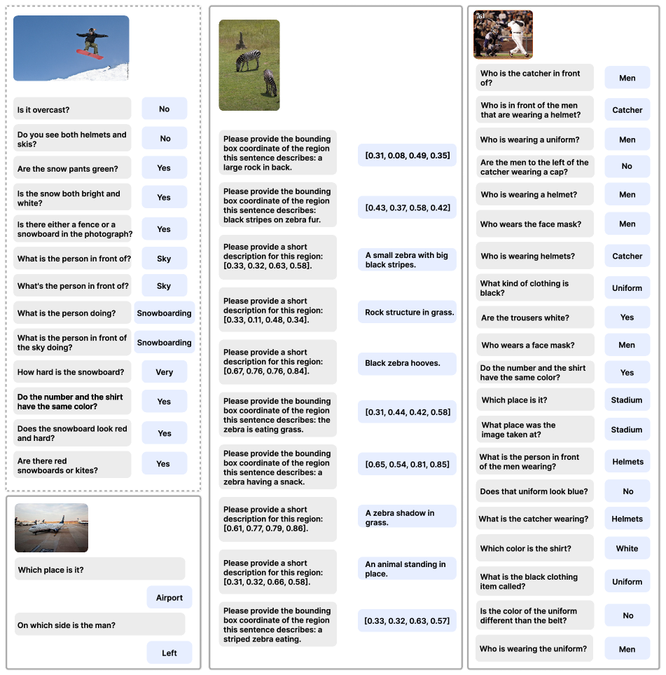
Figure 10: GQA. Top-left: A sample from GQA [13]. Remaining panels show top three influential samples selected using the specialist influence ranking step.

Figure 11: VizWiz. Top-left: A sample from VizWiz [10]. Remaining panels show top three influential samples selected using the specialist influence ranking step.

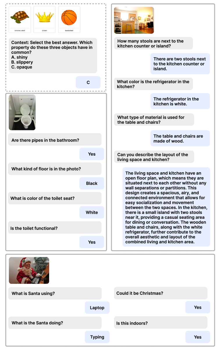
Figure 12: SQA. Top-left: A sample from SQA [25]. Remaining panels show top three influential samples selected using the specialist influence ranking step.

Figure 13: TextVQA. Top-left: A sample from TextVQA [37]. Remaining panels show top three influential samples selected using the specialist influence ranking step.

Figure 14: Pope. Top-left: A sample from Pope [21]. Remaining panels show top three influential samples selected using the specialist influence ranking step.

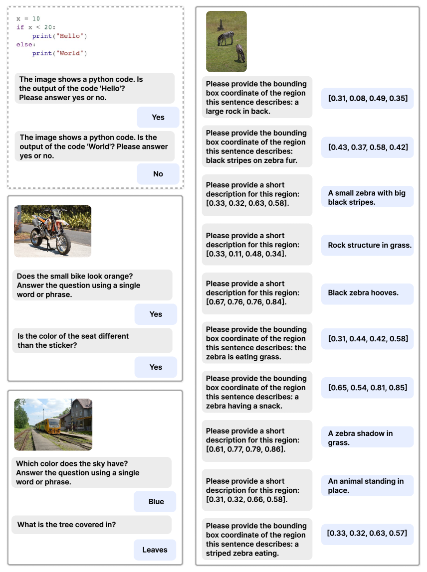
Figure 15: MME. Top-left: A sample from MME [7]. Remaining panels show top three influential samples selected using the specialist influence ranking step.

Figure 16: MMBench (en). Top-left: A sample from MMBench (en) [47]. Remaining panels show top three influential samples selected using the specialist influence ranking step.

Figure 17: MMBench (cn). Top-left: A sample from MMBench (cn) [47]. Remaining panels show top three influential samples selected using the specialist influence ranking step.

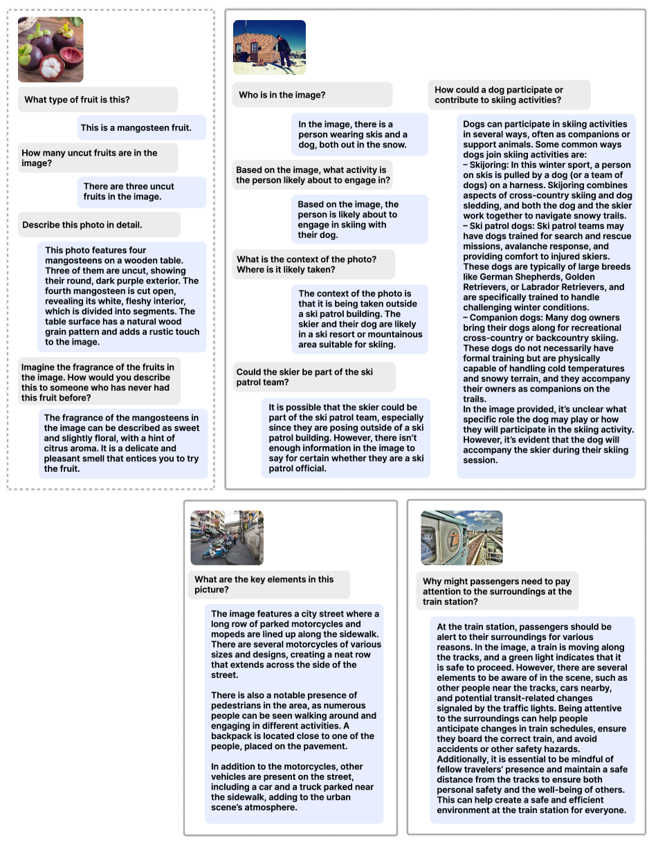
Figure 18: LLaVA-W Bench. Top-left: A sample from LLaVA-W Bench [23]. Remaining panels show top three influential samples selected using the specialist influence ranking step.

Figure 19: Generalist. We show top three influential samples selected after the generalist step.

References

- Abbas et al. [2023] Amro Abbas, Kushal Tirumala, Dániel Simig, Surya Ganguli, and Ari S Morcos. Semdedup: Data-efficient learning at web-scale through semantic deduplication. arXiv preprint arXiv:2303.09540, 2023.
- Alayrac et al. [2022] Jean-Baptiste Alayrac, Jeff Donahue, Pauline Luc, Antoine Miech, Iain Barr, Yana Hasson, Karel Lenc, Arthur Mensch, Katherine Millican, Malcolm Reynolds, et al. Flamingo: a visual language model for few-shot learning. Advances in Neural Information Processing Systems, 35:23716–23736, 2022.
- Brown et al. [2020] Tom Brown, Benjamin Mann, Nick Ryder, Melanie Subbiah, Jared D Kaplan, Prafulla Dhariwal, Arvind Neelakantan, Pranav Shyam, Girish Sastry, Amanda Askell, et al. Language models are few-shot learners. Advances in neural information processing systems, 33:1877–1901, 2020.
- Bukharin and Zhao [2023] Alexander Bukharin and Tuo Zhao. Data diversity matters for robust instruction tuning. arXiv preprint arXiv:2311.14736, 2023.
- Chen et al. [2024] Ruibo Chen, Yihan Wu, Lichang Chen, Guodong Liu, Qi He, Tianyi Xiong, Chenxi Liu, Junfeng Guo, and Heng Huang. Your vision-language model itself is a strong filter: Towards high-quality instruction tuning with data selection. arXiv preprint arXiv:2402.12501, 2024.
- Deng et al. [2024] Zhiwei Deng, Tao Li, and Yang Li. Influential language data selection via gradient trajectory pursuit. 2024.
- Fu et al. [2023] Chaoyou Fu, Peixian Chen, Yunhang Shen, Yulei Qin, Mengdan Zhang, Xu Lin, Zhenyu Qiu, Wei Lin, Jinrui Yang, Xiawu Zheng, et al. Mme: a comprehensive evaluation benchmark for multimodal large language models. corr abs/2306.13394 (2023), 2023.
- Gadre et al. [2024] Samir Yitzhak Gadre, Gabriel Ilharco, Alex Fang, Jonathan Hayase, Georgios Smyrnis, Thao Nguyen, Ryan Marten, Mitchell Wortsman, Dhruba Ghosh, Jieyu Zhang, et al. Datacomp: In search of the next generation of multimodal datasets. Advances in Neural Information Processing Systems, 36, 2024.
- Goyal et al. [2017] Yash Goyal, Tejas Khot, Douglas Summers-Stay, Dhruv Batra, and Devi Parikh. Making the v in vqa matter: Elevating the role of image understanding in visual question answering. In Proceedings of the IEEE conference on computer vision and pattern recognition, pages 6904–6913, 2017.
- Gurari et al. [2018] Danna Gurari, Qing Li, Abigale J Stangl, Anhong Guo, Chi Lin, Kristen Grauman, Jiebo Luo, and Jeffrey P Bigham. Vizwiz grand challenge: Answering visual questions from blind people. In Proceedings of the IEEE conference on computer vision and pattern recognition, pages 3608–3617, 2018.
- Hammoudeh and Lowd [2024] Zayd Hammoudeh and Daniel Lowd. Training data influence analysis and estimation: A survey. Machine Learning, 113(5):2351–2403, 2024.
- Hu et al. [2021] Edward J Hu, Yelong Shen, Phillip Wallis, Zeyuan Allen-Zhu, Yuanzhi Li, Shean Wang, Lu Wang, and Weizhu Chen. Lora: Low-rank adaptation of large language models. arXiv preprint arXiv:2106.09685, 2021.
- Hudson and Manning [2019] Drew A Hudson and Christopher D Manning. Gqa: A new dataset for real-world visual reasoning and compositional question answering. In Proceedings of the IEEE/CVF conference on computer vision and pattern recognition, pages 6700–6709, 2019.
- Johnson [1984] William B Johnson. Extensions of lipshitz mapping into hilbert space. In Conference modern analysis and probability, 1984, pages 189–206, 1984.
- Kaplan et al. [2020] Jared Kaplan, Sam McCandlish, Tom Henighan, Tom B Brown, Benjamin Chess, Rewon Child, Scott Gray, Alec Radford, Jeffrey Wu, and Dario Amodei. Scaling laws for neural language models. arXiv preprint arXiv:2001.08361, 2020.
- Kembhavi et al. [2016] Aniruddha Kembhavi, Mike Salvato, Eric Kolve, Minjoon Seo, Hannaneh Hajishirzi, and Ali Farhadi. A diagram is worth a dozen images. In Computer Vision–ECCV 2016: 14th European Conference, Amsterdam, The Netherlands, October 11–14, 2016, Proceedings, Part IV 14, pages 235–251. Springer, 2016.
- Koh and Liang [2017] Pang Wei Koh and Percy Liang. Understanding black-box predictions via influence functions. In International conference on machine learning, pages 1885–1894. PMLR, 2017.
- Lee et al. [2024] Jaewoo Lee, Boyang Li, and Sung Ju Hwang. Concept-skill transferability-based data selection for large vision-language models. arXiv preprint arXiv:2406.10995, 2024.
- Li et al. [2024] Baiqi Li, Zhiqiu Lin, Wenxuan Peng, Jean de Dieu Nyandwi, Daniel Jiang, Zixian Ma, Simran Khanuja, Ranjay Krishna, Graham Neubig, and Deva Ramanan. Naturalbench: Evaluating vision-language models on natural adversarial samples. arXiv preprint arXiv:2410.14669, 2024.
- Li et al. [2023a] Junnan Li, Dongxu Li, Silvio Savarese, and Steven Hoi. Blip-2: Bootstrapping language-image pre-training with frozen image encoders and large language models. arXiv preprint arXiv:2301.12597, 2023a.
- Li et al. [2023b] Yifan Li, Yifan Du, Kun Zhou, Jinpeng Wang, Wayne Xin Zhao, and Ji-Rong Wen. Evaluating object hallucination in large vision-language models. arXiv preprint arXiv:2305.10355, 2023b.
- Liu et al. [2024a] Haotian Liu, Chunyuan Li, Yuheng Li, and Yong Jae Lee. Improved baselines with visual instruction tuning. In Proceedings of the IEEE/CVF Conference on Computer Vision and Pattern Recognition, pages 26296–26306, 2024a.
- Liu et al. [2024b] Haotian Liu, Chunyuan Li, Qingyang Wu, and Yong Jae Lee. Visual instruction tuning. Advances in neural information processing systems, 36, 2024b.
- Liu et al. [2024c] Zikang Liu, Kun Zhou, Wayne Xin Zhao, Dawei Gao, Yaliang Li, and Ji-Rong Wen. Less is more: Data value estimation for visual instruction tuning. arXiv preprint arXiv:2403.09559, 2024c.
- Lu et al. [2022] Pan Lu, Swaroop Mishra, Tanglin Xia, Liang Qiu, Kai-Wei Chang, Song-Chun Zhu, Oyvind Tafjord, Peter Clark, and Ashwin Kalyan. Learn to explain: Multimodal reasoning via thought chains for science question answering. Advances in Neural Information Processing Systems, 35:2507–2521, 2022.
- Maharana et al. [2023] Adyasha Maharana, Prateek Yadav, and Mohit Bansal. D2 pruning: Message passing for balancing diversity and difficulty in data pruning. arXiv preprint arXiv:2310.07931, 2023.
- Maini et al. [2024] Pratyush Maini, Skyler Seto, He Bai, David Grangier, Yizhe Zhang, and Navdeep Jaitly. Rephrasing the web: A recipe for compute and data-efficient language modeling. arXiv preprint arXiv:2401.16380, 2024.
- Marion et al. [2023] Max Marion, Ahmet Üstün, Luiza Pozzobon, Alex Wang, Marzieh Fadaee, and Sara Hooker. When less is more: Investigating data pruning for pretraining llms at scale. arXiv preprint arXiv:2309.04564, 2023.
- Masry et al. [2022] Ahmed Masry, Do Xuan Long, Jia Qing Tan, Shafiq Joty, and Enamul Hoque. Chartqa: A benchmark for question answering about charts with visual and logical reasoning. arXiv preprint arXiv:2203.10244, 2022.
- Mathew et al. [2021] Minesh Mathew, Dimosthenis Karatzas, and CV Jawahar. Docvqa: A dataset for vqa on document images. In Proceedings of the IEEE/CVF winter conference on applications of computer vision, pages 2200–2209, 2021.
- Mathew et al. [2022] Minesh Mathew, Viraj Bagal, Rubèn Tito, Dimosthenis Karatzas, Ernest Valveny, and CV Jawahar. Infographicvqa. In Proceedings of the IEEE/CVF Winter Conference on Applications of Computer Vision, pages 1697–1706, 2022.
- Mindermann et al. [2022] Sören Mindermann, Jan M Brauner, Muhammed T Razzak, Mrinank Sharma, Andreas Kirsch, Winnie Xu, Benedikt Höltgen, Aidan N Gomez, Adrien Morisot, Sebastian Farquhar, et al. Prioritized training on points that are learnable, worth learning, and not yet learnt. In International Conference on Machine Learning, pages 15630–15649. PMLR, 2022.
- Paul et al. [2021] Mansheej Paul, Surya Ganguli, and Gintare Karolina Dziugaite. Deep learning on a data diet: Finding important examples early in training. Advances in neural information processing systems, 34:20596–20607, 2021.
- Pruthi et al. [2020] Garima Pruthi, Frederick Liu, Satyen Kale, and Mukund Sundararajan. Estimating training data influence by tracing gradient descent. Advances in Neural Information Processing Systems, 33:19920–19930, 2020.
- Radford et al. [2021] Alec Radford, Jong Wook Kim, Chris Hallacy, Aditya Ramesh, Gabriel Goh, Sandhini Agarwal, Girish Sastry, Amanda Askell, Pamela Mishkin, Jack Clark, et al. Learning transferable visual models from natural language supervision. In International conference on machine learning, pages 8748–8763. PMLR, 2021.
- Rajbhandari et al. [2020] Samyam Rajbhandari, Jeff Rasley, Olatunji Ruwase, and Yuxiong He. Zero: Memory optimizations toward training trillion parameter models. In SC20: International Conference for High Performance Computing, Networking, Storage and Analysis, pages 1–16. IEEE, 2020.
- Singh et al. [2019] Amanpreet Singh, Vivek Natarajan, Meet Shah, Yu Jiang, Xinlei Chen, Dhruv Batra, Devi Parikh, and Marcus Rohrbach. Towards vqa models that can read. In Proceedings of the IEEE/CVF conference on computer vision and pattern recognition, pages 8317–8326, 2019.
- Sorscher et al. [2022] Ben Sorscher, Robert Geirhos, Shashank Shekhar, Surya Ganguli, and Ari Morcos. Beyond neural scaling laws: beating power law scaling via data pruning. Advances in Neural Information Processing Systems, 35:19523–19536, 2022.
- Tong et al. [2024] Shengbang Tong, Ellis Brown, Penghao Wu, Sanghyun Woo, Manoj Middepogu, Sai Charitha Akula, Jihan Yang, Shusheng Yang, Adithya Iyer, Xichen Pan, et al. Cambrian-1: A fully open, vision-centric exploration of multimodal llms. arXiv preprint arXiv:2406.16860, 2024.
- Wu et al. [2022] Carole-Jean Wu, Ramya Raghavendra, Udit Gupta, Bilge Acun, Newsha Ardalani, Kiwan Maeng, Gloria Chang, Fiona Aga, Jinshi Huang, Charles Bai, et al. Sustainable ai: Environmental implications, challenges and opportunities. Proceedings of Machine Learning and Systems, 4:795–813, 2022.
- x.ai [2024] x.ai. Introducing Grok 1.5v: The Latest Advancement in AI, 2024. [Online; accessed 14-November-2024].
- Xia et al. [2024] Mengzhou Xia, Sadhika Malladi, Suchin Gururangan, Sanjeev Arora, and Danqi Chen. Less: Selecting influential data for targeted instruction tuning. arXiv preprint arXiv:2402.04333, 2024.
- Yang et al. [2022] Shuo Yang, Zeke Xie, Hanyu Peng, Min Xu, Mingming Sun, and Ping Li. Dataset pruning: Reducing training data by examining generalization influence. arXiv preprint arXiv:2205.09329, 2022.
- Yu et al. [2024] Simon Yu, Liangyu Chen, Sara Ahmadian, and Marzieh Fadaee. Diversify and conquer: Diversity-centric data selection with iterative refinement. arXiv preprint arXiv:2409.11378, 2024.
- Yu et al. [2023] Weihao Yu, Zhengyuan Yang, Linjie Li, Jianfeng Wang, Kevin Lin, Zicheng Liu, Xinchao Wang, and Lijuan Wang. Mm-vet: Evaluating large multimodal models for integrated capabilities. arXiv preprint arXiv:2308.02490, 2023.
- Zhang et al. [2024] Ge Zhang, Xinrun Du, Bei Chen, Yiming Liang, Tongxu Luo, Tianyu Zheng, Kang Zhu, Yuyang Cheng, Chunpu Xu, Shuyue Guo, et al. Cmmmu: A chinese massive multi-discipline multimodal understanding benchmark. arXiv preprint arXiv:2401.11944, 2024.
- Zhang et al. [2023] Yuanhan Zhang Bo Li-Songyang Zhang, Wangbo Zhao Yike Yuan Jiaqi Wang, Conghui He Ziwei Liu Kai Chen, Dahua Lin Yuan Liu, and Haodong Duan. Mmbench: Is your multi-modal model an all-around player. arXiv preprint arXiv:2307.06281, 2, 2023.