Moments and saddles of heavy CFT correlators
Abstract
We study the operator product expansion (OPE) of identical scalars in a conformal four-point correlator as a Stieltjes moment problem, and use Riemann-Liouville type fractional differential operators to transform the correlation function into a classical moment-generating function. We use crossing symmetry to derive leading and subleading relations between moments in and in the “heavy” limit of large external scaling dimension, and combine them with constraints from unitarity to derive two-sided bounds on moment sequences in and the covariance between and . The moment sequences which saturate these bounds produce “saddle point” solutions to the crossing equations which we identify as particular limits of correlators in a generalized free field (GFF) theory. This motivates us to study perturbations of heavy GFF four-point correlators by way of saddle point analysis, and we show that saddles in the OPE arise from contributions of fixed-length operator families encoded by a decomposition into deformed higher-spin conformal blocks. To apply our techniques, we consider holographic correlators of four identical single scalar fields perturbed by a bulk interaction, and use their first few moments to derive Gaussian weight-interpolating functions that predict the OPE coefficients of interacting double-twist operators in the heavy limit. We further compute tree-level perturbations on saddles in 1/2 BPS Wilson line defect correlators in planar SYM, making predictions about deformations of families of long operators.
1 Introduction
The conformal bootstrap Ferrara:1973yt ; Polyakov:1974gs ; Poland_2019 aims to constrain or even solve conformal field theories (CFT) by systematically imposing consistency conditions and symmetries. CFTs not only describe universality classes of systems at their second-order phase transitions, but they also describe the space of asymptotic observables for a quantum field theory (QFT) in Anti de Sitter (AdS) space of one dimension higher Maldacena:1997re ; Gubser:1998bc ; Witten:1998qj . In the AdS/CFT correspondence, the conserved stress tensor on the boundary CFT is dual to a bulk graviton, allowing us to study theories of quantum gravity by probing their dual CFT.
The structure of a CFT arises from its convergent and associative operator product expansion (OPE). By performing appropriate conformal transformations, we can bring two local operators arbitrarily close to each other so that their product can be decomposed into an infinite number of primary operators of the form
| (1) |
where are OPE coefficients extracted from the normalization of a three-point correlator, and is a differential operator which constructs a conformal multiplet from the primary.
Considering a conformal four-point function of identical scalars, we can take the OPE between two pairs of operators and decompose it as
| (2) |
We identify as a conformal block, parameterized by the scaling dimension and spin quantum numbers of . In Euclidean signature , while in Lorentzian signature and are independent real numbers. In general, the analytic continuation of the block maps , where is the double cut plane. The conformal block is a group harmonic which resums the contributions of an irreducible representation, labeled by its lowest-weight (or “primary”) vector , to the correlation function. The ability to produce such a decomposition is a consequence of Plancherel’s theorem for the conformal group bams/1183531812 . Most importantly, this decomposition allows us to describe any four-point correlator by a countable set of “CFT data,” which consists of the spectrum and OPE coefficients . Taking a union of these data for all four-point correlators in a given theory then uniquely describes all the local observables of the CFT.111Holographically, the OPE encodes the distribution of intermediate states exchanged in a scattering process through the AdS bulk, with each term in the sum of eq. (2) associated with a Witten exchange diagram.
An important constraint arises from the associativity of the OPE, where we can equate decompositions of the correlator in different channels, corresponding to different choices of pairs of operators. This property gives rise to the s-t channel “crossing equation”
| (3) |
where , and
| (4) |
is the crossing vector and are the standard conformal cross ratios. Another important constraint on the decomposition arises for unitary CFTs, and imposes that the OPE coefficients are real so that all are positive. Applying a basis of functionals to this sum rule and using the positivity of allows one to rule out certain CFT spectra by preparing a functional that produces a contradiction after acting on the proposed spectrum. Functionals which are constructed to prove an optimal bound such as the maximum allowed scalar gap or a given OPE coefficient are called “extremal functionals,” and encode the spectrum of the correlator which saturates such a bound in their root structure. One can implement the search for such a functional as a semi-definite program (SDP) which can be solved numerically El-Showk:2012vjm .
In the past decade, there has been tremendous growth in the numerical conformal bootstrap program yielding crucial insights into the structure of CFTs. Notably, we can now compute precise quantum numbers of a large number of operators in the 3d Ising CFT El_Showk_2012 ; El-Showk2014-ce ; Kos:2016ysd ; chang2024bootstrapping3disingstress , the O(N) vector models Kos:2013tga ; Chester:2019ifh ; Chester:2020iyt , Gross-Neveu-Yukawa CFTs Atanasov:2022bpi ; Erramilli2022-yi , and place nontrivial constraints on 3d gauge theories Albayrak2021-td ; Chester2016-tp . These results are obtained by combining SDP constraints involving a variety of “light” correlators that relate the OPEs of relevant and marginal operators in the theory. In each of these correlators, the OPE is dominated by light operators, so the parameter space subject to optimization is sufficiently small and the numerics are tractable.
A class of observables that remains somewhat elusive to this treatment are four-point correlators which involve some number of irrelevant operators. One reason for this is that correlation functions involving operators with scaling dimension much larger than the unitarity bound tend to be dominated by a large number of conformal blocks with scaling dimensions of the same order. This makes the parameter space subject to optimization much larger than can be effectively analyzed numerically, with extremal functionals from SDP converging very slowly for larger values of . If one were able to overcome these difficulties, correlators of irrelevant operators would give us better access to the large scaling dimension data of the CFT. These data can give us insights into the mechanics of strongly-interacting multiparticle and black hole states in the dual gravitational bulk – unraveling the mysteries of which is a crucial goal in the study of quantum gravity.
To better clarify our observables of interest in the context of holography, consider a scalar operator in a -dimensional boundary CFT. The scaling dimension of this operator is related to the mass of the corresponding bulk field by
| (5) |
where we work in units where the AdS curvature . Taking larger implies a larger mass, but how do we quantify “heavy”? When the boundary CFT has a conserved stress tensor, there is a finite central charge to which we can compare the scaling dimensions of boundary operators.222The squared OPE coefficient describing the three point coupling of two identical scalar operators to the stress tensor is where is the central charge of the theory. In the case of , we can justly consider the operator “heavy,” and its insertion on the boundary distorts the AdS metric Mishra2024-mr . The exact bulk description of these operators is theory dependent, and they may be dual to strings, branes, or black holes emerging from the asymptotic boundary. Computing boundary correlators of these operators holographically requires corrections from the presence of these extended surfaces in the bulk. For , the boundary insertions are more generally viewed as insertions of massive particles, Kaluza-Klein (KK) modes, or perhaps de-localized “blobs” Fardelli2024-ra ; Abajian2023-xw (depending on the presence of a large parameter) and can be in principle computed with Witten diagrams. In this work, we will generally refer to any correlator with external scaling dimension as heavy, and we will refer to the limit as the heavy limit.
The majority of extant literature on heavy dynamics focuses on the case of heavy-heavy-light-light correlators, see e.g. Abajian2023-xw ; Grabovsky2024-bg . These correlators are amenable to a variety of holographic approaches where the heavy states source a background geometry in AdS space and light operators are approximated as “probes” which travel along geodesic paths in the deformed spacetime. These correlators can also be related to the two-point functions of light operators in a CFT at finite temperature, which describes the dynamics of a light operator scattering off an AdS black hole with the same Hawking temperature Iliesiu2018-od .
These approaches fail in the case of heavy-heavy-heavy-heavy correlators where each of the operators is both sourcing and backreacting off of each other’s geometry. Not only is this problem difficult within a known theory, but attempting to study them from the bootstrap perspective seems similarly intractable as there is very little known about how to effectively truncate the parameter space that characterizes them. Unlike light correlators whose behavior is well approximated by a finite number of quantum numbers describing the low-lying spectrum, there is no such immediate “microscopic” description that captures the physics of heavy dynamics where the OPE is dominated by a large number of similarly heavy operators.
Finite temperature calculations have been used to derive high-energy asymptotics of CFT data, including heavy-heavy-heavy OPE coefficients and the asymptotic density of states for a general dimension CFT as a function of scaling dimension and spin Benjamin2023-qo . These techniques work by describing thermal correlators as local operators coupled to background fields governed by a local “thermal” effective action on compact geometries. On a torus, this effective action describes a thermal partition function with inverse temperature and spin fugacity , which parametrizes “twists” of along the thermal circle.
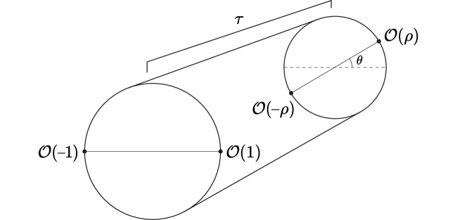
When a four-point correlator of identical scalars is dominated by operators with large scaling dimension, the conformal block decomposition resembles a thermal partition function for the subset of states that show up in the OPE of the external operators. In this limit, the effective inverse temperature is controlled by the separation of operator pairs along the cylinder , a 1-dimensional spin fugacity is controlled by the angular separation of operator pairs along the cylinder, and the OPE coefficients resemble state degeneracy factors. This leads us to consider a similar space of observables to characterize heavy correlators as we do more general thermal systems, where standard macroscopic observables such as average energy and total angular momentum can be computed by applying appropriate functionals to the correlator.
In this paper, we will study correlators of identical scalars with using a three-fold approach. First, in section 2 we define and construct Riemmann-Liouville type fractional differential operators in 1, 2, and 4 dimensions that extract the principal series eigenvalues from a conformal block. These operators resolve the 8-fold degeneracy in the eigenspace of the quadratic Casimir of the conformal group into four subspaces related by a discrete “rotation” symmetry of the Casimir eigenvalue. Additionally, we construct the analogous operators in general dimension that extract these eigenvalues from the asymptotic conformal block at large scaling dimension. When applied to a CFT correlator of identical scalars, these “principal series operators” compute global averages over CFT data in a given kinematic regime, weighted by powers of the quantum numbers of scaling dimension and total angular momentum . Exponentiating the principal series operators allows one to transform a correlator into a classical moment-generating function (MGF), which implies a unique decomposition of a correlator into a moment sequence that obeys the conditions from the Stieltjes moment problem in certain kinematic limits.
Second, in section 3 we directly use constraints from crossing and unitarity to derive bounds and relations between these moments, focusing on the “heavy” limit of . Previous studies have analyzed constraints from crossing in this limit Kim2015-sg and have derived leading-order relations between moments in scaling dimension Paulos2016-mh . We further extend these results by deriving subleading relations between moments, including those which involve some power of total angular momentum. We then combine these relations with positivity constraints from unitarity to derive a leading bound on the covariance of the quantum numbers and in any crossing-symmetric OPE. The leading relations from crossing and a corollary of the existence condition for the Stieltjes moment problem allows us to compute two-sided bounds on the leading behavior of moments in the heavy limit.
In section 4 we then re-sum the moment sequences that saturate the leading bounds to derive extremal saddle-point solutions to the crossing equations in the heavy limit. This leads us to our last fold, where we relate these solutions to particular limits of correlators in a generalized free field (GFF) theory, and show that saddle points in the OPE distribution correspond to a decomposition into higher-spin (HS) conformal blocks which organize contributions to the GFF OPE by operators involving a fixed number of elementary scalar fields. These HS conformal blocks are known to provide a tractable finite basis for correlators with weakly broken higher-spin symmetry Alday2016-kz , and we present a tree-level procedure to “unmix” deformations on this basis given a number of correlators involving lighter operators in the theory. Further, we show that the derived measures we obtain by matching only the second moment of these HS conformal blocks (and their deformations) satisfy the properties of a function which, up to a determined factor, interpolates the weights of operators in the OPE.333The weight of an operator in a OPE is given by and is thus dependent on the kinematics of the correlator. We show that these weight-interpolating functions (WIFs) provide quantitative predictions of OPE coefficients as a continuous function of scaling dimension for correlators of sufficiently large external scaling dimension in a variety of perturbative examples. A corollary to this observation is that the weights of operator families of fixed length become distributed along Gaussian distributions, therefore reducing the space of variables that describes them to their first few moments.
Finally, in section 5 we apply our tree-level saddle unmixing procedure to correlators of displacement operators in the 1/2 BPS Wilson line defect CFT in planar SYM, and provide some qualitative predictions about how long families of operators deform under gravitational interactions in the bulk. We conclude with a discussion of our results in section 6.
2 Principal series operators
Let us begin by considering the conformal group, with generators
| (6) | ||||
The -dimensional Lorentzian conformal algebra is isomorphic to the algebra of , with its generators identified as
| (7) | ||||
Here, and are non-compact and generate dilatations and longitudinal Lorentz boosts respectively agarwal1 . These generators give rise to unitary principal series representations labeled by continuous weights , for , and an irreducible representation of . Together, the pair specifies a weight of , and is the length of the first row in its Young Tableaux diagram Kravchuk_2018 . To simplify our discussion, we will take to be the trivial representation so that is a rank traceless symmetric tensor, and suppress the label .
The principal series representation is an eigenvector of the quadratic Casimir of the conformal group , with eigenvalue
| (8) |
This eigenvalue has a discrete symmetry group isomorphic to the dihedral group , which includes three subgroups given by the actions
| (9) |
Rewriting and (or alternatively and ) we see that generates rotations and generates reflections of the square, giving the standard group presentation
| (10) |
Since , the eigenspace of is 8-fold degenerate and its eigenbasis is obtained by applying group elements of to . The resulting basis is given by
| (11) |
In this section, we will explicitly construct additional operators and in and which extract the principal series eigenvalues, and respectively, from eigenvectors of . These operators decompose the quadratic Casimir as
| (12) |
and allow us to resolve the 8-fold degeneracy of the eigenspace into 4 independent 2-fold degenerate subspaces given by
| (13) |
Elements within a subspace are related by precomposing a rotation with , and the remaining degenerate subspaces are related by the rotation .
Concretely, we will be constructing by studying the actions of integral transforms on conformal blocks . Conformal blocks can be schematically written as
| (14) |
where are “external” local scalar operators at marked points , and is an “exchanged” local primary operator with quantum numbers . Conformal blocks are group harmonics for a conformal correlator of the form , repackaging contributions of irreducible representations with lowest weight vector to the correlator.
When the external scalar operators are identical, the conformal block satisfies the second-order differential equation
| (15) |
where
| (16) |
and
| (17) |
The “Dolan-Osborn” coordinates are related to the standard conformal invariant cross ratios as and . In and , exact solutions to the differential equation are given by Dolan:2000ut ; Dolan:2003hv
| (18) | ||||
In general dimension, conformal blocks also admit the radial representation Hogervorst:2013sma
| (19) |
where
| (20) |
is the regulated conformal block, and
| (21) | ||||
are radial coordinates.
Here, is a meromorphic function in with containing a series of poles in below the unitarity bound associated with zero-norm vectors Kos:2013tga ; Penedones_2016 . Explicitly,
| (22) |
and
| (23) |
with a Gegenbauer normalization factor, and indexes the infinite set of null states. While the form of is not known in closed form, it can be computed by a recursion relation order-by-order in powers of . Due to the presence of the poles, the contribution of the null states is suppressed as , allowing us to determine the asymptotics of the conformal blocks for in general dimension as
| (24) |
2.1 Exact operators
In song2023compactform3dconformal , a modified Riemann–Liouville fractional derivative was introduced with the following transformation property on conformal blocks
| (25) |
where
| (26) |
The prefactor of (25) vanishes for , so this transformation acts as zero on the conformal block associated with the exchange of the identity operator. By conjugating an infinitesimal rescaling of by this transformation, we can construct an operation which extracts the principal series eigenvalue
| (27) |
In and 4, the conformal block factorizes up to a power of into a symmetric sum of products of conformal blocks, so it is possible to construct an analogous operator that transforms a conformal block into a sum of power-laws in .
We denote this transformation
| (28) |
and define
| (29) |
It is easy to check that the operators satisfy
| (30) |
| (31) |
in 2 and 4 dimensions, where must be applied twice to extract an eigenvalue from the conformal block due to its antisymmetry under .444When is applied once, the conformal block is transformed to a chirally antisymmetric block which flips signs under . Indeed, it is this symmetry of the quadratic Casimir under that renders unable to resolve the remaining 2-fold degeneracy of the eigenspace.
2.2 Asymptotic operators
In addition to being able to construct the -operators exactly in and 4 dimensions, we can also use the known form of the conformal block at large to construct analogous asymptotic operators in general dimension, which we will call .
Upon a Weyl transformation of , we introduce the cylinder coordinates
| (32) |
| (33) |
so that and . Since , we have
| (34) |
Applying this operator to the radial form for the conformal block and solving for the action of gives
| (35) |
We can now use the known form of to find
| (36) |
which acts as multiplication by a -independent function on normalizable contributions, and zero on non-normalizable contributions, so that the asymptotic result is consistent with the exact result. Combining with (34), we find
| (37) |
which satisfies as .
We can attempt a similar procedure to compute , however one quickly finds that does not act as a function independent of on the conformal block, telling us there is additional mixing of differential operators when is applied twice. Furthermore, since a conformal block is not an eigenfunction of , we cannot use an analogous operator equation to compute alone.
Instead, we will start by constructing an operator that acts as by using the property of the Gegenbauer polynomial
| (38) |
with
| (39) |
We can then construct by dressing with a term which subtracts off the remaining commutator
| (40) |
Since is second order, the commutator is a first-order differential operator which we compute directly, giving
| (41) |
which satisfies
| (42) |
in the limit of .
Assembling the -operators with the appropriate dimension-dependent shifts then gives the final result
| (43) | ||||
3 Moments of the OPE
A classical moment problem studies the moment map which takes a positive distribution function on to the sequence of moments given by
| (44) |
Given such a sequence, we would like to determine: 1) if such a positive measure exists, 2) if the moment sequence uniquely determines . If these two conditions are satisfied, then the moment sequence is said to be “determinant.” For many determinant moment sequences, there exists a moment-generating function which satisfies for all . Moreso, the measure can be uniquely recovered by applying the inverse Laplace transform
| (45) |
For an in-depth discussion on the classical moment problem in mathematics literature, see the standard texts by Akhiezer alma99671493502466 , Shohat & Tamarkin Shohat1943ThePO , and Schmüdgen gradtextsmomentproblem .
3.1 Stieltjes moment problem
The classical Stieltjes moment problem is the special case when . Since this requires both the support and measure to be positive, we have the condition for all polynomials and . This implies that the (shifted) Hankel matrices of the moment sequences are positive semi-definite555This condition can be strengthened to positive definiteness () when the measure is continuous or . for all . Sylvester’s criterion for the positivity of symmetric matrices states that this condition is satisfied if the determinants of all leading minors are positive. If moment sequences obey these positivity conditions, then such a functional exists. Moreso, moment sequences which satisfy Hankel matrix positivity form a convex subset of all positive real sequences called the moment cone schmüdgen2020lecturesmomentproblem .
A sufficient (but not necessary) criteria for uniqueness is given by Carleman’s condition for the Stieltjes problem, which states that a moment sequence is determinant if
| (46) |
For the cases of interest in this paper, moments are power-law bounded so that for all for some constant . Therefore, moment sequences satisfy Carleman’s condition and are determinant.
3.1.1 Generalized moment-generating functions
A generalized moment-generating function is defined by a moment kernel and a sequence of linear functionals which take . The moment kernel and linear functionals define a moment map which takes a measure to a real moment sequence via
| (47) |
This construction is essentially equivalent to the classical case when considering a moment kernel that is an eigenfunction of a linear operator with eigenvalue . Linear functionals in this case are given by
| (48) |
If , we can study the measure pulled back to coordinates with the moment decomposition:
| (49) |
Provided that the integrand is still positive definite over the support , the resulting moments will satisfy Hankel matrix positivity by the same argument as the previous section. After computing the moment-generating function and taking the inverse Laplace transform, the original measure can be recovered by dividing out the Jacobian factor and changing variables.
3.2 Four-point correlators in CFT
Correlation functions of four identical scalar operators in a CFT can be viewed as a special case of a generalized moment-generating function
| (50) |
where is a conformal block, is a kinematic prefactor, and
| (51) |
is a “raw” discrete measure which contains -distributions at the quantum numbers of primary operators in the OPE, weighted by squared and normalized OPE coefficients .666We denote the normalization of two-point correlators . The measure is positive definite in a unitary CFT. We organize operators in the OPE by their quadratic Casimir eigenvalue, , rather than their spin. We can set to pull back to the Casimir eigenvalue. For , this map is bijective on .
The sequence of linear functionals we choose to produce moments of this measure is given by applying shifted -operators to the correlator and evaluating at some so that conformal blocks are positive over all quantum numbers. In this work, we will focus on measures in the diagonal limit and evaluate at . The resulting moments are given by
| (52) | ||||
To simplify our notation, we will introduce the weighted measure :
| (53) |
which is defined so that . Applying the functional in (52) then gives , so that our moment map produces a classical moment sequence for the measure over and . Weighted measures with the script omitted refer to evaluation at the diagonal self-dual point . We label these moments as , or with only scaling moments as .
3.3 Bounds from crossing and unitarity
An associative OPE yields scalar four-point functions which are invariant under permutations of the external operators, expressed by equating
| (54) |
with the OPE channels labeled s, t, and u respectively. This condition constitutes crossing symmetry, and subtracting the OPE decompositions of two of the channels gives rise to a consistency condition on CFT data expressed as the sum rule. The s-t crossing sum rule is
| (55) |
where we have multiplied through by as a convention so that the crossing vector is antisymmetric under . Taylor expanding the crossing vector around gives a countable set of constraints order-by-order in the series777We denote evaluation at the self-dual point by suppressing dependence on position variables.
| (56) |
with all terms of even identically vanishing by the antisymmetry of . We can further decompose each Taylor coefficient into a choice of basis which corresponds with a given moment map
| (57) |
where we have assumed the internal sum is sufficiently convergent (or finite) so that it commutes with the functional. The ability to do such an operation depends on the choice of moment map, as not all basis functions lead to convergent expansions which can be swapped with the OPE.
This is a subtle point, and indeed the series which decomposes the above constraints into the classical moment basis proposed in this paper has a finite radius of convergence due to the presence of poles in below the unitarity bound in the conformal block. By truncating the number of these poles, we can approximate the conformal block as a power law times a meromorphic function in . We can separate this meromorphic function into a finite number of polynomial and non-polynomial moments with a partial fraction decomposition, and show that the non-polynomial moments are subleading in the heavy limit of . Thus, the majority of our analysis in this paper will focus on heavy correlators, so that we may approximate
| (58) |
where is a polynomial in and with maximal degree . Exact analysis of the crossing equation in terms of the classical moment basis is necessary for correlators with small . This problem can be approached numerically, and we plan to pursue this direction in upcoming work.
Let us consider a constraint coefficient at odd order . We will suppress the structure of the regulated conformal block and explicitly separate out the pre-factor of the block. We compute
| (59) | ||||
where is the multinomial coefficient, is the rising factorial, and terms with suppressed dependence imply evaluation at the self-dual point. It is obvious that the terms with give polynomials in with no dependence on spatial dimension, spin, or any meromorphic functions of . These terms can be computed exactly and give relations between polynomial moments in scaling dimension, . Additionally, these terms contain a homogenous polynomial in which dominates the relations between moments of heavy correlators, or when primary operators of large scaling dimension dominate the OPE.
Lastly, we have terms which contain factors of the form
| (60) |
with . The first term on the RHS is exactly computable and gives a degree polynomial in . The terms in the sum which contain only polynomial factors of give relations between a finite number classical moments at a given derivative order and will be referred to as asymptotic constraints, since they arise from a crossing equation prepared with conformal blocks of the form .
On the other hand, the second term on the RHS is not known in closed form in general dimensions, and can only be computed up to a finite pole order by recursion relations for a given spin. We can compute such a term for a large number of spins and derivatives numerically to find the bound
| (61) |
which holds for all scaling dimensions greater than the unitarity bound at a given spin as well as at the identity. More specifically, we find the value at the identity is for any non-zero derivative order.
The non-polynomial terms are approximated by a degree rational function in and contain poles at and below the unitarity bound. Therefore,
| (62) |
for greater than the unitarity bound at a given spin.
These observations allow us to compute a universal bound on the first scaling dimension moment from the constraint coefficient at order , given by
| (63) |
where the left-most term comes from the asymptotic regulated conformal block, using both the fact that the full regulated conformal block is bounded by the asymptotic, and that it is explicitly zero at the identity so that we may subtract off from the normalization . We see that as , , or that the average scaling dimension of our measure approaches a universal linear term depending only on the scaling dimension of the external operators. This result extends to moments the asymptotic constraints from “reflection symmetry” previously observed in Kim2015-sg ; Paulos2016-mh . The order at which this statement fails to be projective, in that it involves terms which are not of the form , is subleading in the heavy limit. This is seen by the fact that for , which is the case for a unitary CFT.
In order to obtain bounds on higher moments, we need to utilize our constraints from unitarity, i.e. Hankel matrix positivity, and develop a systematic way of studying asymptotic crossing constraints. We first want to show that moments of the form for some less than or equal to the unitarity bound do not dominate constraints from crossing for any , so that we can safely analyze only the asymptotic constraints. We can start by subtracting off the identity from the OPE decomposition, so that all other operators lie above the unitarity bound and their regulated conformal blocks can be approximated, up to orders of , by the asymptotics
| (64) | ||||
The classical moments of the subtracted OPE distribution are equivalent to those of the total distribution as the identity has a scaling dimension of , so it does not contribute to for . For the normalization, we can explicitly subtract off the identity contribution giving . The benefit of working with this subtracted distribution is that we can estimate inverse moments such as without worrying about any operators at causing such terms to diverge.
The inverse moments satisfy completely analogous Hankel matrix positivity constraints since they are still positive functions on . That said, we will only need to estimate . It is easy to check that iff , so that we can bound the inverse moment by the gap in scaling dimension as
| (65) |
Thus, for any , the inverse moments which approximate non-polynomial terms in the regulated conformal block contribute at most corrections to the relations between classical moments given by the asymptotic constraints. We prove stronger bounds for inverse moments in appendix A by using the leading bounds on polynomial moments obtained in the following section 3.3.1.
3.3.1 Leading-order bounds in the heavy limit
Now that we have addressed the non-asymptotic constraints, we can direct our attention to deriving leading-order bounds on the normalized moments in the heavy limit. It is easy to compute a lower bound with Hankel matrix positivity alone, using the fact that for all integers . Sylvester’s criterion for the first non-trivial minor determinant then gives the necessary constraint that
| (66) |
for all . By inducting on and dividing both sides by the appropriate power of , we find888This constraint is Jensen’s inequality.
| (67) |
While this statement is easy to derive, its implications are powerful, telling us that .
Let us consider the set of constraints that arise in the diagonal limit of , so that we can study scaling moments alone without moments in . Later, we will show that constraints obtained without first taking the diagonal limit are identical in the limit, so that constraints that involve spin moments do not affect the results we derive in this section. Additionally, we will be considering projective relations between moments, i.e. all terms involved will be of the form , so we will not subtract the identity contribution from our measure functional. Indeed, this analysis fails at subleading order, as the identity operator lies below the unitarity bound and is thus not well approximated by the asymptotic block.
For all odd, we have the diagonal constraints
| (68) |
where , and
| (69) |
Since these factors are all , any term which contains a derivative with respect to the asymptotic regulated conformal block is subleading in the limit, thus we can focus on the constraints at :
| (70) |
where plugging in the asymptotics and gives
| (71) |
Note that while we have not assumed that , the fact that the highest power of multiplying is always for all forces the leading-order constraint coefficients to be homogeneous polynomials in . Since the form of the constraint coefficient is invariant under an arbitrary rescaling , the moments transform homogeneously as well with .
To compute an upper bound, we solve a finite set of polynomial equations recursively at each order :
| (72) |
and
| (73) |
Solutions to these equations saturate Hankel matrix positivity bounds and satisfy the leading crossing symmetry constraints, so we use the convexity of the allowed region to conclude
| (74) |
So far we considered the leading behavior of the moments in the heavy limit . We can also use similar methods to obtain constraints on subleading terms in the large expansion. We describe some of these constraints in appendix B.
3.3.2 Spin moments and covariance bound
In this subsection, we verify some assumptions made for our leading analysis, and compute a new result giving a two-sided bound on the leading term in the covariance between and . Namely, we show at that
-
•
Moments involving some power of are always subleading in the heavy limit, and therefore the leading constraints obtained by first restricting to the diagonal limit are as strong as those obtained from a more general expansion of the crossing vector.
-
•
Computing a general expansion of the crossing vector in cylinder coordinates around gives rise to the first non-trivial constraint relating spin moments and scaling moments at order .
-
•
Combining the above constraint with the leading bounds on moments gives the following bound on the leading term in covariance:
(75)
To see the first point, let us revisit our constraint coefficient from eq. (59). If we assume every term which contains a derivative with respect to the regulated conformal block is subleading, then we can take and and study only leading constraints of the form
| (76) |
Each term is symmetric in and , so we can set , , and sum over to obtain
| (77) |
which gives equivalent constraints between the moments and powers of as we obtained when we took the diagonal limit before taking derivatives.
Now we would just like to show that terms that involve any derivative of the regulated conformal block are indeed subleading in the limit. To see this, recall that derivatives of the asymptotic regulated conformal block are order polynomials in , so we need to bound the growth in of moments of the form . From investigations of the lightcone limit, we know that the behavior of the OPE at large spin is controlled by the t-channel identity and thus tends towards the GFF as Fitzpatrick:2012yx ; Komargodski2012-na ; Pal:2022vqc ; vanrees2024theoremslightconebootstrap .
Let us consider splitting the OPE into high- and low-spin sectors with some cutoff value of the spin Casimir :
| (78) |
We claim that the measure functional at very large corresponds to the generalized free theory and is controlled by the term , and the measure functional contains all the anomalous data. We can bound , as the distribution which maximizes a given moment over this compact region is simply a delta function at .
On the other hand, consider the free theory moments of given by
| (79) | ||||
Resumming the leading terms into a moment-generating function and taking the inverse Laplace transform gives an approximation of the OPE distribution over the spin Casimir for a heavy GFF as a gamma distribution, with shape parameter and scale :
| (80) |
Integrating this measure from our cutoff and normalizing accordingly gives an estimate for the moments:
| (81) | ||||
Therefore, in the heavy limit. Moreover, if we take , then the moment of the measure will dominate the total moment so we can bound
| (82) |
for all in the heavy limit.
Since we are only concerned with bounding the leading-order behavior, let us take the upper bound of for some positive constant . The objects we need to bound are terms of the form as these are the terms which we expect to be subleading in the heavy limit. To do this, we use the Cauchy-Schwartz inequality
| (83) |
where , , and defines an inner product on a set of random variables . Based on the maximal growth rate we derived for and , it is easy to see that this implies and therefore for some positive constants . Lastly, since one requires the application of at least two derivatives to the regulated conformal block to obtain a power of , any term in the constraint coefficient which involves a power of may grow at most as , and is therefore subleading in the heavy limit.
Since terms in the constraint coefficient involving spin moments are always subleading in the heavy limit, it is impossible to isolate them from terms involving moments in scaling dimension at the same order in . This yields a number of mixed constraints relating averages over spin, scaling dimension, and their products. One way of organizing these constraints is by expanding around cylinder coordinates, where we can view constraints as arising perturbatively from the self-dual point by ‘pulling’ and ‘twisting’ operator pairs along the cylinder.
Consider the crossing equation in coordinates, with the identity subtracted, as
| (84) |
where we construct from the asymptotic conformal blocks at large . Expanding both sides around and evaluating at gives the following constraints at order and respectively:
| (85) |
and
| (86) | ||||
The order constraint has no dependence on spin, and is identical to those derived from the diagonal limit, so the first non-trivial constraint on spin moments from crossing is given by eq. (86).
Using our spin constraint from crossing and the leading-order behavior of moments, we can derive a bound on the leading term in the covariance of and . First, let . Plugging this in and taking the heavy limit gives
| (87) |
From our diagonal constraints and bounds from unitarity, we know that and , implying the bound on spinning/mixed moments
| (88) |
We can rephrase this as a bound on the covariance , which takes the form
| (89) |
4 Saddles and deformations
In this section, we will focus on OPE distributions over scaling dimension, defining
| (90) |
The moments of this distribution can be computed from a moment-generating function as .
Let us first consider the formal limit of , so that normalized moments are sharply bounded as in eq. (74) as for all . The upper bound is saturated by the moment-generating function
| (91) |
Similarly, the lower bound is saturated by the moment-generating function
| (92) |
These “extremal” moment-generating functions correspond to the asymptotic measures
| (93) |
and
| (94) |
While these measures are clearly unphysical, in that they do not give rise to an exactly crossing-symmetric OPE for a finite , the locations of the -distributions should be viewed as describing the approximate weights and locations of the dominant operator contributions to the OPEs of extremely heavy correlators.
In general, an asymptotic moment-generating function will sit between these, with
| (95) |
Considering the structure as a sum of exponentials, we can write down a “heavy” ansatz as
| (96) |
with positive weights . Here we interpret as the locations of “saddle points” associated with sharp peaks in the OPE distribution whose locations scale linearly with . As implied by our upper bound, we expect that is our heaviest saddle and we take as the saddle associated with the s-channel identity contribution. The term in the exponential represents subleading corrections to this saddle point approximation that broaden and skew each -distribution while maintaining its average at .
We would like to further specify the form of this saddle decomposition for correlators with large identical external scaling dimension prepared in different theories. To this end, we’d like to first discuss the OPE saddle structures that arise for correlators in a generalized free theory. We’ll see that OPE saddles are in 1-to-1 correspondence with higher-spin (HS) conformal blocks that decompose free correlators, representing families of multi-twist operators involving a fixed number of elementary fields. Lastly, we will present a framework for studying individual deformations on OPE saddles from tree-level perturbative correlators.
4.1 Generalized free fields and higher-spin conformal blocks
A generalized free field (GFF) theory provides an important playground for studying the structure of heavy correlators. Our analysis considers different ways one can construct a heavy operator in the theory. The bulk action of a GFF is given by a massive free scalar field
| (97) |
In this theory, all correlators in the boundary CFT can be computed with Wick contractions, which correspond to the disconnected exchange of the field(s) through geodesic paths in the AdS space bulk. Additionally, we can define normal ordered products of fields by taking their OPE and subtracting off singular terms. The scaling dimension of the product field is given by . Since we can vary both and take an arbitrary number of normal ordered products, we can construct operators with identical scaling dimensions but different OPEs.
Consider a four-point correlator of the form
| (98) |
where we have normalized by the product of two-point correlators
| (99) |
The full correlator can be computed directly with Wick contractions corresponding to the propagation of fields along geodesic paths in AdS space between points , , and . The result is
| (100) |
where
| (101) |
are the so-called “higher-spin” (HS) conformal blocks introduced in Alday2016-kz .
Focusing our analysis on the OPE distribution over scaling dimension, we will restrict to the 1d kinematics of the diagonal limit and define and . In these variables, the 1d correlator reads
| (102) |
To compute the decomposition of in terms of 1d conformal blocks, we will make use of the -space identity from Hogervorst:2017sfd :
| (103) |
Let us warm up with the case, or the GFF correlator of the elementary primary field :
| (104) |
Using the above identity, one can verify the decomposition into 1d blocks:
| (105) |
with
| (106) |
where we recognize the only contributing operators as the double-twist family with scaling dimensions and OPE coefficients
| (107) |
Moving on to general , we note that each term in the sum over higher-spin conformal blocks is characterized by an overall power of , giving rise to a 1d conformal block decomposition with a gap at . Applying eq. (103) to all the terms at each unveils a highly degenerate operator spectrum with for positive integer . Thus, the OPE is of the form
| (108) |
For a given , the coefficients admit a closed form in terms of hypergeometric functions obtained from the expansion coefficients of eq. (103):
| (109) |
In the heavy limit of , becomes peaked around and is very well approximated as . We can re-sum these dominant contributions to obtain the asymptotic correlator of
| (110) |
Note that if we further restrict kinematics to the Euclidean section with , then the powers of fall off exponentially in the heavy limit, and we find
| (111) |
This asymptotic correlator has a spectrum with scaling dimensions for and , rather than the standard double integer spaced spectrum we observed in the full correlator. This is because terms which are subleading in the heavy limit serve to subtract off the “odd spin” operators that arise in the leading-order result.
Based on the form of the full 1d correlator given in (102), we expect our classical moment-generating function to be of the form
| (112) |
where are the unnormalized classical moment-generating functions of an individual higher-spin conformal block.
In the heavy limit, these leading moments read
| (113) |
Resumming these leading terms into the classical moment-generating function gives
| (114) |
or that each higher-spin conformal block is associated with a single saddle located at . The locations of these saddles coincide with dominant operator contributions at .999For , the asymptotic conformal block is a constant and the locations of OPE saddles are just the peaks of the bare OPE coefficients at . This can also be made apparent if one directly studies the OPE coefficients multiplied by conformal blocks of dimension . However, the result obtained here required no knowledge of the exact CFT data, and instead emerged only from a leading-order moment analysis of the higher-spin conformal blocks.
With this leading moment-generating function for each saddle known, let us consider the moments of the total measure generated by . To make contact with our previous bootstrap results from crossing, we will restrict our analysis here to the self-dual point . If we take at , the higher-spin conformal block and the saddles are located at for . Additionally, the value of the correlator goes as
| (115) |
First, we consider the case in the heavy limit. We find the total normalized th moments are given by , which match the leading upper bounds . Additionally, if we fix and take the long limit of , we find , which match the moments saturating the leading lower bound we derived. This gives meaning to the extremal moment sequences and as the and limits of the GFF correlator, respectively. The latter case is more universal in that these moments are recovered for all in the long limit, while the sequence is only recovered when . We note that the lack of a saddle associated to the identity in is a result of non-identity operators dominating the correlator in this limit. This dominance is apparent as as .
We can refine our picture of these saddles by estimating the terms in the exponential of our moment-generating function. A simple way to do this is by making a smooth ansatz for the derived measure obtained by taking the inverse Laplace transform of , and matching the moments which parametrize it. As we will show in the next section, the best ansatz for saddles in the heavy limit is given by a Gaussian
| (116) |
where
| (117) | ||||
are the mean and standard deviations of each saddle, with the position dependence of the higher-spin conformal blocks suppressed.
At the level of the moment-generating function, this gives
| (118) |
where the terms correct the skew and higher moments associated with this ansatz.
We now just need to compute the associated with each saddle, and plug the result back into the form of the total measure
| (119) |
We expect these Gaussian corrections for the derived measure to only be valid near the heavy limit, when the OPE distribution can be approximated as a finite sum of saddle points. Therefore, it suffices to study the moments of the terms in which are leading in the heavy limit for Euclidean configurations, namely
| (120) |
The first and second moments for these terms can be computed exactly in 1d and are given by
| (121) | ||||
where .
Additionally, we can use our asymptotic operators to compute the approximate result in general dimension
| (122) | ||||
as .
With these moments in hand, there are a few key facts to point out. First, the moments generated by our Gaussian match the leading terms we obtained from the -distribution result. The subleading terms slightly shift and widen the leading -distributions, and we can study the standard deviations of each saddle. At these are given by
| (123) |
On the other hand, the locations of the saddles are separated by intervals of . This means that, for a fixed , taking the heavy limit results in saddles that become relatively spaced apart, while fixing and taking the long limit results in saddles that overlap and merge to form one large mass around . The standard deviation of this collective saddle is controlled by the symmetry factors in the sum over , and is given by
| (124) |
Notably, if we fix the total external scaling dimension , we find at leading order
| (125) |
with the total standard deviation vanishing as .
This further demonstrates that our measure tends towards a -distribution at in the limit of , giving rise to the measure which nearly saturates the lower bound of moment space, .
4.2 Weight-interpolating functions
In section 4.1, we used a Gaussian ansatz to model some of the properties of saddles based on their mean, variance, and normalization. This choice is made for two main reasons:
-
•
A Gaussian is the maximum entropy distribution for a fixed mean and variance, making it the “most probable” distribution that matches those low-lying moments.
-
•
Up to a determined factor, our derived Gaussian measures converge uniformly to the exact weights of local operators in the spectrum of each saddle in the heavy limit.
The second bullet will be the focus of this section, and we begin with a definition.
Consider the weighted OPE distribution over scaling dimension at ,
| (126) |
A weight-interpolating function (WIF) satisfies
| (127) |
for all in the discrete support of . Such a function is not unique, and one can be directly constructed from the measure as
| (128) |
for all less than the difference in scaling dimension between any two operators in the OPE. The resulting WIF is not generically smooth or continuous. If the OPE spectrum is uniformly spaced in , then it is possible to construct a linear WIF which is piecewise continuous over scaling dimension by smearing over an appropriate kernel.
Let us explicitly construct a linear interpolation function for the weights of an equally spaced discrete ’target’ distribution where is the spacing between each -distribution and are some positive weights. need not be normalized. A linear interpolating function for this distribution should satisfy for all and for .
Such a function can be obtained by convolution with a triangle function
| (129) |
where
| (130) |
If we were to compute the moments of , we would see:
| (131) |
or that the moments of the linear interpolation function are approximately those of the target distribution multiplied by the spacing between -distributions, up to a correction by a sub-subleading moment. In the context of our problem, where moments are organized in an expansion around , this implies , where is the moment sequence of an approximately linear WIF.
This property is also satisfied by the derived Gaussian measure we used to study the OPE distribution in GFF correlators when operators in the spectrum are separated by . Thus, we find
| (132) |
in the heavy limit, where is a derived measure consisting of a sum over Gaussian saddles of the form (116). In addition to checking this agreement graphically in a number of examples, we also prove uniform convergence for the simple case of and , or when the target weights are known as a simple analytic function for , the derived measure is a single Gaussian, and the normalization rapidly approaches in the heavy limit. To condense notation, we will adopt the convention of .
We say uniformly converges to the exact weights if for every there exists a such that for all and
| (133) |
To derive asymptotics in the heavy limit, let us re-parametrize by setting where parametrizes the number of standard deviations (of order ) one is from the mean of the leading saddle. Plugging this in and expanding around gives
| (134) |
and
| (135) |
Subtracting these results and bounding the difference gives
| (136) |
for all , where . Thus, converges uniformly to the exact weights in the heavy limit, with errors of order .
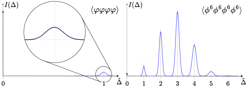
To give some examples, in the LHS of fig. 2 we plot the exact weights of double-twist operators in the OPE for a large external scaling dimension against the Gaussian WIF we computed from its moments. In the RHS, we plot the WIF for the OPE expressed as a sum over Gaussians, tuning the scaling dimension of a single field such that .
4.3 Perturbations and saddle unmixing
Next, we would like to consider what happens when we perturb away from the above picture, e.g. by introducing an AdS bulk interaction. Under perturbations in small coupling , correlators admit an expansion of the form
| (137) |
At leading order, we expect that perturbations affect only the operators exchanged in the free OPE, picking up anomalous scaling dimensions and OPE coefficients of the form
| (138) | ||||
where indexes each of the non-identity saddles. To align with our previous conventions, we identify . For , the OPE coefficients pick up an additional rescaling, which at leading order is simply the symmetry factor
| (139) |
To see this, first consider the property of the 3pt correlator in the free theory
| (140) |
obtained by computing Wick contractions, with the symmetry factor arising from two -pick- vertex factors and one edge permutation factor. We will set as the smallest such that the RHS is non-vanishing. Combining the transformation property of the 3-pt correlator with the normalization factors and , we find
| (141) | ||||
The same transformation property also arises at due to the derivative rule arising from bulk perturbations Heemskerk2009-mb :
| (142) |
Combining this transformation property of OPE coefficients and the fact that no additional states are entering the OPE allows us to decompose similarly to as
| (143) |
We then define
| (144) |
as the “deformed” higher-spin conformal block representing the correction to each saddle, and in our previous conventions.
This observation gives rise to an interesting inverse problem: given a collection of perturbed correlators, compute for . In other words, we want to find the coefficients such that
| (145) |
for any .
To do this, we can first write
| (146) |
Separating out the term and replacing
| (147) |
gives
| (148) |
We can continue this replacement recursively. Let us denote the coefficients appearing at the ’th iteration as , where, for example
| (149) | ||||
Repeating this procedure for the term reveals a simple recursion relation between -coefficients for
| (150) |
and we identify the -coefficients as the special case .
These coefficients are easy to compute recursively, however they also admit the convenient “diagrammatic” representation
| (151) |
with for all . The tuplet represents a kind of Young tableau, explicitly given by
| (152) |
To provide a few illustrative examples (for ) we have
| (153) | ||||
Putting it all together, we find that the first few -coefficients are given by
| (154) | ||||
Equipped with these coefficients and a set of correlators for , we can now compute the deformed HS conformal blocks that decompose at first order in the coupling. The moments of these deformed HS blocks characterize how the collective behavior of a family of fixed-length operators is perturbed by an interaction. If we plug the moments for each deformed HS block into the Gaussian ansatz for the OPE measure, the induced shifts in the weights, mean, and variance of each saddle give a coarse-grained description of how the OPE is deformed by an interaction. We will look at an explicit example of this in the next section.
5 Applications
Given a correlator, one would like to extract the underlying CFT data, which enables the calculation of critical exponents and provides holographic insights into bulk physics. Light correlators tend to be governed by a small number of light states, whereas heavy correlators are dominated by numerous heavy states. This complexity of the high-dimension spectrum poses a challenge, especially in heavy perturbative correlators, where unmixing the CFT data remains difficult even when using the Lorentzian inversion formula. These challenges become more pronounced in holographic theories with non-renormalizable bulk interactions, where heavy states are highly sensitive to the UV behavior.
The approach we offer to gain insights into this challenging physics is to treat the CFT data as a coarse-grained distribution over scaling dimensions and spin, and examine how interactions affect the descriptive statistics of this smooth distribution rather than focusing on a few discrete data points. By utilizing the basis of HS conformal blocks and their associated OPE distributions, we can gain new perspectives into the physics of heavy CFT correlators, dual to the bulk physics of heavy states, advancing our understanding of quantum many-body physics in gravitational theories.
The coarse-grained OPE distributions we compute offer not only qualitative insights but can also be useful quantitatively. In section 4.2, we showed that rescaled Gaussian measures, or WIFs, converge uniformly to the exact weights of the GFF spectrum in the heavy limit. In the interacting case, Gaussian WIFs computed from the perturbed data remain highly accurate approximations of the exact weights in the heavy limit, even at finite coupling. We dub this phenomenon “Gaussianization” and verify that saddles perturbed by bulk contact diagrams with an arbitrary number of derivatives Gaussianize as .
5.1 Bulk contact interactions
Let us consider perturbing the AdS bulk action (97) by a contact interaction containing derivatives:
| (155) |
This interaction has been extensively studied at tree level in AdS2 Bianchi2021-li ; Knop2022-qh , and the anomalous dimensions of double-twist families with scaling dimension have been computed in closed form to be
| (156) | ||||
This formula admits a simple asymptotic form as , giving
| (157) |
This asymptotic behavior will be sufficient for our analysis of the OPE measure at , since the OPE is dominated by double-twist operators with as . Note that for , this interaction is a relevant operator in an AdS2 bulk, so anomalous dimensions vanish as Fitzpatrick2010-wk . This means that heavy saddles are robust to perturbations by this operator and remain well-approximated by the free theory result. On the other hand, the operator for is irrelevant, so anomalous dimensions grow with . This means there are non-trivial deformations on heavy saddles which we can measure by studying how moments are shifted in the presence of the interaction. The marginal case of results in being a constant, and saddles are merely shifted by an amount proportional to . In all cases, for the anomalous dimensions go as , therefore we can take to cancel out the large dependence so that for all .
Neglecting the corrections, we can compute the moments explicitly as
| (158) |
This procedure may be thought of as a resummation of tree-level data into the moment variables, with deviations from the true all-loop order moments arising at order . In practice, eq. (158) is computed by summing over operator contributions in a large window around the saddle at . We then plug these moments into the Gaussian ansatz in eq. (116) evaluated at , and multiply by the appropriate factor to produce our desired perturbed WIF.
We can approximate by considering the spacing between operators around the saddle point, i.e. when for . Let . Taking and , we find
| (159) | ||||
The numerator of the anomalous term is for operator spacings around the saddle, so . Neglecting this error term, we can simply set to obtain our perturbed WIFs in the heavy limit.
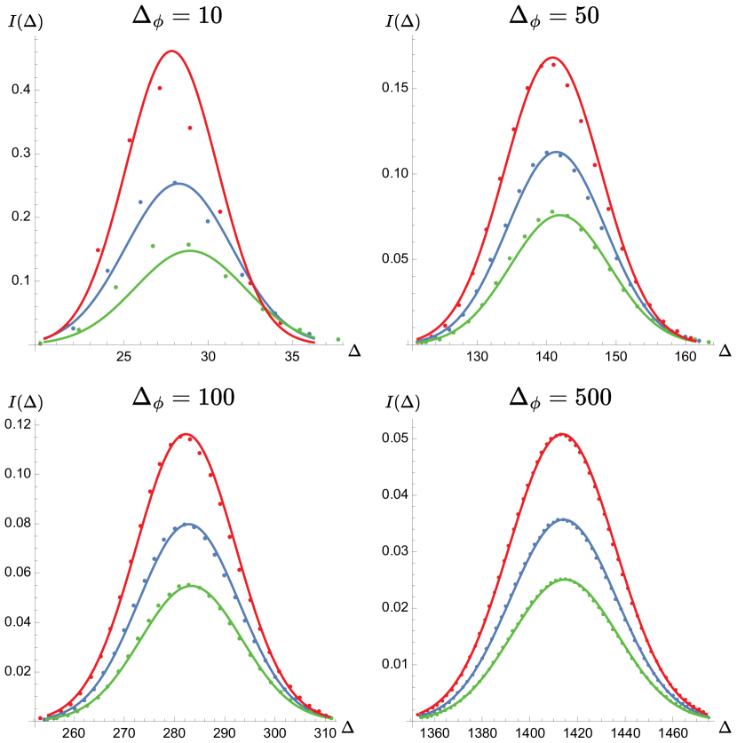
We find that the perturbed WIFs computed using the Gaussian approximation do an excellent job of capturing the shape of the spectrum at all perturbative values of , and even at values. To illustrate this, in fig. 3 we plot these perturbed WIFs against the spectrum of with an contact interaction for different values of the coupling and external scaling dimension. We present a sequence of plots with to show how both free and interacting spectra tend towards Gaussian WIFs in the heavy limit. The required moments were directly computed by summing over a window of 120 operators around , capturing the contributions of operators within standard deviations from the mean.
One way to quantitatively test the “Gaussianity” of the perturbed OPE distribution is by comparing its exact higher moments to those predicted by the Gaussian ansatz. Namely, we can ask whether
| (160) |
as for all . If this condition is satisfied, then we can reconstruct the WIF for a given perturbed OPE density from the first two exact moments as a Gaussian in the heavy limit, with corrections arising at sub-subleading order in .
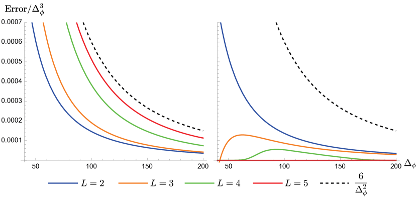
In fig. 4, we check these error terms for the moment of a correlator perturbed by contact interactions with derivatives, and find that this condition is indeed satisfied for all we were able to feasibly check. Perhaps more interestingly, the rate at which the OPE distribution associated with a different interaction Gaussianizes is dependent on the sign of the coupling. We find that higher-derivative interactions Gaussianize slower with a negative coupling, while lower-derivative interactions Gaussianize slower with a positive coupling. A more in-depth analytical investigation of this saddle Gaussianization would be extremely interesting, as would tests of Gaussianization at higher order in the coupling.
5.2 Unmixing saddles in the 1/2 BPS Wilson line defect CFT
In this section we give another application of our methods, which is to use our tree-level saddle unmixing procedure to study 4-point correlators of products of displacement operators in the half-BPS Wilson line defect CFT appearing in the planar limit of SYM. The works ferrero1 ; ferrero2 computed correlators of the form up to 1-loop order for arbitrary . As a proof of concept, we will utilize their tree-level results for correlators with to compute first-order perturbations on each of the moments associated with the non-identity saddles showing up in the free correlator. We then plug these perturbed moments into our Gaussian approximation for each saddle, giving a novel picture of how the total OPE distribution is deformed by bulk gravity. Moreso, when the coupling is taken away from a perturbative regime, we highlight the phenomena of “saddle collapse,” giving rise to resonances in the OPE associated with heavy multi-parton states.
While the majority of these results give a coarse-grained picture, they allow us to develop a crucial intuition of how interactions in the bulk affect the collective behavior of operator families in the OPE, without requiring computation of anomalous data of any individual operators. This provides a new way of ascertaining bulk physics from boundary correlators.
At large ’t Hooft coupling , the four-point function of admits the expansion ferrero2
| (161) |
where
| (162) |
for , and
| (163) |
with the polynomial given by
| (164) |
Here and are superconformal cross ratios, given by
| (165) |
where are the R-symmetry cross ratios.
To make contact with our previous results, we will fix , so that , , and . These kinematics give rise to a reflection positive configuration so that the OPE distribution is positive definite over scaling dimension. In these kinematics, the tree-level perturbation on the correlator is given by
| (166) | ||||
To obtain the leading interacting higher-spin conformal blocks we use (145) to write the formula
| (168) |
To simplify our analysis, we will consider the OPE distribution at and compute moments by applying our asymptotic operator. This approach yields approximate moments for the lighter saddles, but quickly becomes nearly exact when considering the heavy saddles whose OPE distribution is centered around a large .
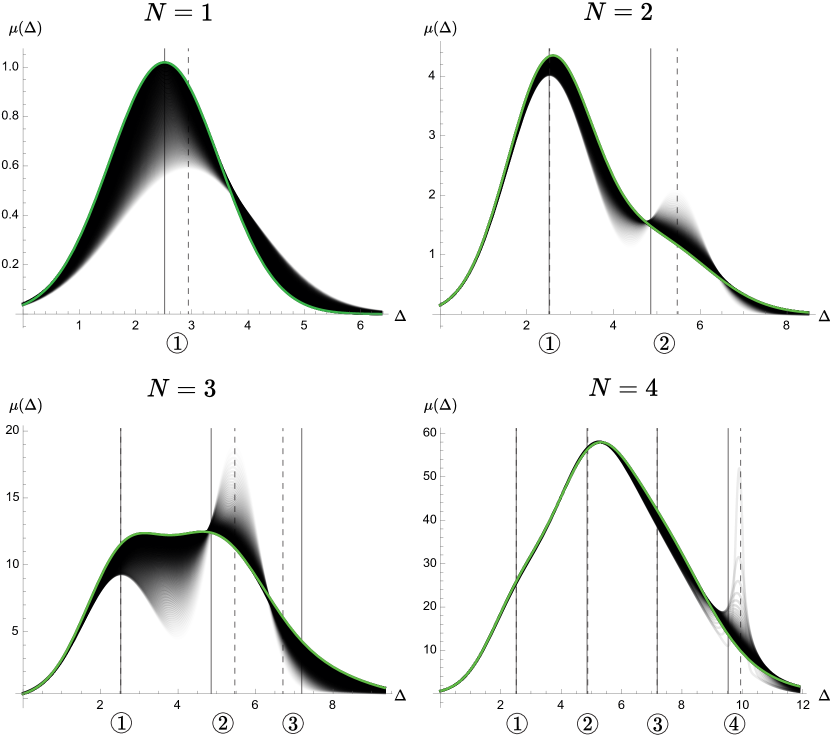
In our Gaussian approximation scheme, each of the -indexed OPE saddles are characterized by their weight, , their mean and their variance . In table 1, we tabulate these for the first 9 saddles at tree level at large ’t Hooft coupling. We note the regular sign oscillations for the heavy saddles. For the standard deviations , negative perturbations give rise to the phenomena of “saddle sharpening” when the coupling is taken away from the perturbative regime. Similarly, positive perturbations cause saddles to flatten and contribute less to the total OPE distribution. We plot the resulting corrections to the derived OPE distributions as the coupling is increased for in fig. 5, where one can see these interesting features.
Studying the anomalous dimensions of multi-parton operators tells us about the nature of bulk physics. Namely, the presence of an attractive bulk interaction causes the energies of multi-parton states to decrease as they become more energetically favorable field configurations. Similar conclusions can be ascertained from the signs of anomalous moments, but through a seemingly opposite effect. Namely, we notice a characteristic “blue shift” of normalized moments such as and . This phenomena occurs due to the enhanced presence of heavy bound states in the distribution of intermediate states exchanged through the bulk. On the other hand, the presence of a repulsive interaction causes a red-shift of moments as light single-particle states start to dominate the OPE.
This effect does not occur uniformly however, with some families of multi-parton operators enhanced and others suppressed when coupled to gravity. This is very apparent when studying the variances of each saddle, where negative perturbations result in the variance going to zero, or the saddle becoming sharply peaked and resembling a resonance in the OPE, and positive perturbations result in the saddle becoming flattened. It would be very interesting to see how this effect is corrected at loop order.
6 Discussion
In this paper, we have proposed the use of classical moments in and as a useful way of repackaging CFT data, focusing on applications for “heavy” correlators of identical scalar operators with . This analysis is dependent on the unitary OPE being encoded by a positive definite measure over scaling dimension and total angular momentum, with the full correlator viewed as a generalized moment-generating function for the OPE distribution.
The latter construction relies on the existence of operators which extract the necessary powers of and from the conformal block, which we construct exactly with Riemann-Liouville-type fractional derivative operators in and , and construct asymptotically with integer-derivative operators for conformal blocks of large scaling dimension in general dimension. The exact operators make use of the transformation introduced by song2023compactform3dconformal , which we dress with an additional factor so that it acts naturally on the prefactor of the 4d conformal block. These operators allow us to easily generate moments using the action
| (169) |
It would be interesting in future work to construct exact operators in general dimensions, as well as their generalizations to mixed correlators and higher-point functions. Such operators would give us even more powerful tools for studying the statistics of CFT data.
Exponentiating , and applying them to a correlator gives the classical moment-generating function associated with the raw OPE distribution, weighted by an additional factor of the conformal block. The existence of this moment-generating function implies the determinancy of the moment sequence we use to characterize the correlator, and the underlying OPE distribution can be obtained via an inverse Laplace transform in the variables . Due to the additional weighting by the conformal block, the moments produced are dependent on the kinematics of the correlator. For some kinematic regimes, namely the Lorentzian self-dual line , the conformal block is positive for all dimensions and spins, so we can study the weighted measure as a positive distribution.
We can use crossing symmetry to constrain moments by Taylor expanding the crossing equation around the diagonal self-dual point and imposing that the coefficients vanish at each order. If we assume that the correlator is dominated by operators away from the unitarity bound, we may use the asymptotic conformal block to derive these constraints, and we obtain polynomial relations between moments at each finite derivative order. Combining these constraints with a lower bound arising from the Hankel matrix positivity of the moment sequence, we find that the leading constraint at large organizes into a homogeneous polynomial in and , implying that moments in tend towards in the large limit. This fact gives a simple constraint on crossing-symmetric OPE distributions in the heavy limit, posed as a vanishing of odd central moments:
| (170) |
This relation was previously explicitly derived in appendix D of Paulos2016-mh to study the flat space limit of AdS, and is a restriction of an approximate “reflection symmetry” of the OPE Kim2015-sg to the diagonal self-dual point of . We combined the constraint of (170) with Jensen’s inequality to derive two-sided bounds on the leading large behavior of normalized moments in :
| (171) |
While this is a novel result in the study of classical moment sequences of correlators, a seemingly related bound was proposed in Sen_2019 (see eq. (5.5)), where geometric “moment” methods were used to derive a window in the OPE guaranteed to include at least one primary operator. It is debatable as to which one of these bounds is “stronger.” On the one hand, the authors of Sen_2019 derived a rigorous statement about the presence of operator(s) in this window, but it does not give information about where operators may be clustered in this window or which operators are contributing most to the OPE. While our bound may not constrain the locations of operators in an exact sense, it does make a strong statement that operators should be dominantly distributed in the OPE around with a maximum variance of , demonstrating how the collective behavior of operator contributions is constrained by the bootstrap. In addition, the two extremal solutions saturating our bounds contain non-identity saddles at and , respectively. In this sense, we view these bounds as complimentary – one proving the existence of individual operators in this window, and the other proving that operators must collectively cluster in this window and dominate the OPE.
We also note that the methods used in Sen_2019 ; Huang2019TheGO are qualitatively similar to ours. Namely, they introduce the sequence of moments given by the Taylor coefficients of the correlator around the diagonal self-dual point. This choice certainly has its benefits, in that crossing can be understood as restricting truncated moment sequences to a hyperplane in the projective moment space. Additionally, one does not require the kind of fractional derivative operators we used to obtain the moments of a correlator. What this method may lack however, is a more direct interpretation of each of the moments in terms of CFT data. This makes it difficult to go from the simple (and exact) constraints from crossing to compelling statements about OPE data which extend those produced by the numerical bootstrap.
Our method has countering strengths. While it is difficult to analytically derive exact constraints on classical moments from crossing, the relations we are able to derive can be directly interpreted as bounds on descriptive statistics of CFT data and give insights into the global structure of the OPE. It would be interesting to further unify our results with those presented in Sen_2019 ; Huang2019TheGO by constructing an explicit mapping between the classical and geometric moment basis along with their relations from crossing. In upcoming work, we plan to extend our analytic study to use semidefinite optimization methods to exactly constrain classical moments, augmenting bounds produced by the standard numerical bootstrap by giving new quantitative insights into the contributions of high-dimension CFT operators.
In addition to deriving a constraint equation for subleading terms of moments in the heavy limit (restricting to diagonal kinematics), we computed a relation between moments in the spin Casimir and scaling dimension and combined them with Hankel matrix positivity to obtain a two-sided bound on the leading term in the covariance
| (172) |
This is an intriguing result that can be thought of as a “generalized” unitarity bound on the behavior of heavy spinning operators in scalar correlators. The standard unitarity bound for spinning operators states that . This naturally suggests that in a unitary OPE we should expect heavy operators to be correlated with operators with higher spin. The lower bound in eq. (172) confirms this fact, and the upper bound additionally states that there is a universal bound on the rate at which average scaling dimension grows with average spin. In future work, we plan to probe this bound in kinematic configurations away from the diagonal self-dual point, focusing on Lorentzian configurations where the OPE may become dominated by larger spin contributions. Such bounds may be useful in understanding the distribution of operators over spin along a given Regge trajectory.
After constraining the allowed moment space for unitary and crossing-symmetric correlators of identical scalars, we wanted to understand where interesting solutions to crossing lie in this moment space, and how one can reconstruct the OPE distribution of a correlator given its low-lying moments. We first computed the “extremal” measures which have moment sequences that saturate the upper and lower bounds of eq. (171), and found they are given by saddle point solutions with equally weighted -distributions at and for the maximal case, and a single -distribution at for the minimal case. These asymptotic solutions to crossing can be obtained by taking different limits of the correlator in a GFF. Namely, the maximal solution is obtained by taking with , and the minimal solution is obtained by fixing and taking . For and finite , we find that the OPE distribution over scaling dimension for this correlator is approximated by non-identity saddle points distributed symmetrically around at the locations for . Each one of these saddles is associated with a “higher-spin” (HS) conformal block, first introduced in Alday2016-kz , which repackages operator families of fixed length , and are holographically dual to multi-parton states in the AdS bulk.
The approximate locations of saddles associated with the HS block decomposition were identified by studying moments of the correlator at leading order in the limit. As one might expect, subleading terms correct these locations and give saddle points a finite width. By truncating computed moments at subleading order in large , the derived measures associated with each saddle become Gaussian distributions with widths of order . A similar effect within the Mellin space decomposition of a tree-level Witten diagram was observed by the authors of Paulos2016-mh in a study of the flat space limit of AdS. When the flat space limit of was taken, the sum over power laws with Gaussian weights sharpened into a -distribution identified with a single massive pole in the flat space S-matrix. The “Gaussianization” we observe for each saddle in the OPE is a larger collective effect, where a sum over conformal blocks with Gaussian weights appear to coalesce into -distributions in the limit.
Up to a factor determined by the operator spacing of the spectrum, these Gaussian approximations for the OPE measure tend to interpolate the exact weights of operators in a given saddle, converging uniformly with errors of order as . We verified this analytically in the free theory, and graphically for theories with an irrelevant bulk contact interaction (focusing on the t-channel identity saddle in the correlator). In both cases, the weight-interpolating functions (WIFs) we derive provide quantitative predictions for OPE coefficients as a function of scaling dimension in a given saddle, using only the first three moments (including the normalization) for each saddle. This illustrates a somewhat uncanny ability of the low-lying moment variables to capture the CFT data of high-dimension operator contributions to the OPE. The caveat of this technique is that the actual locations of individual operators are lost, and the same WIF applies to multiple unique spectra. That said, in correlators whose high-dimension spectrum becomes nearly dense, these WIFs seem to be the best way of predicting this non-universal data as a “coarse grained” description of a large number of operators. It would be useful to study the effects of higher moments such as the skew and kurtosis on these WIFs, and see how precisely one can interpolate the exact weights of the conformal block decomposition. It might also be interesting to formulate a general numerical bootstrap program for heavy correlators by studying crossing constraints on an ansatz written as a sum of (nearly) Gaussian WIFs.
At tree level, we showed that perturbative terms in a correlator of can be decomposed identically to the HS block decomposition of the free correlator. This leads us to consider deformations on HS blocks as a means to reorganize terms in the perturbative correlator, where each deformed HS conformal block encodes how states with a fixed parton number are collectively perturbed by an interaction. By studying correlators for , we are able to unmix perturbative terms to reorganize them into the deformed HS block basis. We contrast this technique with the more ambitious goal of standard operator unmixing, where one desires to compute the individual anomalous data for a set of degenerate operators. It will be interesting to extend this analysis to mixed correlators (or higher-point functions), where one could study the effect of deformations on higher-twist families of operators.
More generally, decomposing correlators into families of operators with fixed length is reminiscent of the cluster expansion of a thermal partition function in small fugacity alma991033040259703276 . These expansions are used to study interacting many-body systems because, unlike a standard perturbative series in small coupling, cluster expansions in are convergent, with each term corresponding to contributions from states involving a fixed number of particles. Similar to our formulation of deformed HS conformal blocks, order terms in the cluster expansion, or -particle “Slater sums,” are expressed graphically as a linear combination of diagrams with connected pieces. Since this cluster expansion is convergent, it could be useful to further import these techniques to the study of CFT. This would invite the possibility of bootstrapping deformed HS blocks, giving us novel insights into the dynamics of long operator families in strongly-interacting theories.
In a recent series of papers ferrero1 ; ferrero2 , the authors unmixed the anomalous data of operators in the 1/2 BPS Wilson line defect in planar SYM, working up to operators with length 6 by studying correlators of displacement operators of the form . The authors note that unmixing the anomalous data of longer operators requires a larger set of correlators to resolve the degeneracy space, making it exceptionally challenging to understand perturbations on operators with very large lengths. Using their tree-level results, our work attempts to probe deformations of families of long operators without such a microscopic description, instead opting to understand how the statistics describing these operator families are perturbed by computing the moments of their associated deformed HS blocks. Our result gives a novel way to describe how exceptionally long families of operators are collectively perturbed, and we tabulated the perturbed means, variances, and weights of saddles in the OPE distribution over scaling dimension.
While we only presented results up to operators of length 18, our technique can be applied to arbitrarily long operators. These results are promising, and currently seem to be the only tractable way of understanding the heavy CFT data in perturbative correlators like these. That said, these results are only computed at tree level and one quickly loses perturbative control when considering operator families with length due to the non-renormalizability of the bulk interaction. In the future, we hope to generalize this procedure to higher-loop order and consider effects from additional operator families entering the OPE. It would be especially exciting to study bulk gravitational physics from the saddle perspective, e.g. the role of exchanged black hole states vs multi-parton states.
One particularly intriguing effect we noticed at tree level was the alternating collapse and resonance of saddles depending on the parity of the saddle index . This effect seems reminiscent of what one may expect from conformal multiplet recombination, where distinct HS multiplets combine via the equations of motion to form a single HS multiplet rychkov2015epsilonexpansionconformalfieldtheory . It may be the case that the saddle collapse we observe here indeed corresponds to those multi-parton states recombining with a set of states with different parton number after interactions are introduced. If we considered e.g. a saddle point analysis of a correlator near the Wilson-Fisher fixed point in dimensions, we might expect a similar saddle collapse to occur when as the set of length 6 operators mixes with length 2 and 4 operators via the relation . Exploring the evolution of saddles in perturbative examples such as this may help to give new insights into the structure of CFT correlators.
Acknowledgements.
We thank Li-Yuan Chiang, Murat Koloğlu, Petr Kravchuk, Tony Liu, Dalimil Mazáč, Alessio Miscioscia, Matthew Mitchell, Ian Moult, Riccardo Rattazzi, Petar Tadić, Yuan Xin, and Xiang Zhao for discussions. The authors were supported by Simons Foundation grant 488651 (Simons Collaboration on the Nonperturbative Bootstrap) and DOE grant DE-SC0017660.Appendix A Bounds on inverse moments
The lower bounds on polynomial moments in (67) allow us to strengthen our bounds on inverse moments for some . To do this, we will introduce a regulator , and bound . First, since , the support of lies above the pole at and contributions are weighted by the tail of the power law . Thus,
| (173) |
Now, observe that
| (174) |
Therefore, we can use Fubini’s theorem to swap the power series and measure functional, and bound each term in the sum with the lower bound of eq. (74):
| (175) | ||||
Taking and multiplying by gives
| (176) |
An equivalent result can be obtained by integrating over the minimal measure :
| (177) |
Appendix B Subleading relations in the diagonal limit
Let us consider subleading constraints on the projective scaling dimension moments, which at large admit an expansion of the form
| (178) |
We can study constraints on the coefficients which arise from the crossing equation by plugging in this ansatz and computing relations order-by-order in . The expansion of 178 is truncated at , as any further subleading terms are related to corrections from the non-asymptotic piece of the regulated conformal block (see appendix A).
To analyze subleading coefficients with , we will scale and and study the terms in the constraint coefficient of order and . Here, the coefficients that show up in the term are related to the coefficients in the term. Going to the diagonal and taking derivatives with respect to , we find the constraint from crossing at order and read
| (179) | ||||
where and . While we have written these constraints separately, they are indeed related at subleading order after plugging in our ansatz (178) and setting .
Expanding each of the terms as a polynomial and replacing for and , we find the constraint
| (180) | ||||
where the first term in the last line is a non-projective constraint, involving a factor not of the form . The remaining terms are all projective and can be expanded with the ansatz (178). Doing so, we recover relations between the coefficients at order and :
| (181) | ||||
with
| (182) |
Note that since with no subleading terms, we have and .
To check this relation, let . At order , we have , and at order 1 we have . This agrees with our previous bound (63) obtained without these general relations.
References
- (1) S. Ferrara, A.F. Grillo and R. Gatto, Tensor representations of conformal algebra and conformally covariant operator product expansion, Annals Phys. 76 (1973) 161.
- (2) A.M. Polyakov, Nonhamiltonian approach to conformal quantum field theory, Zh. Eksp. Teor. Fiz. 66 (1974) 23.
- (3) D. Poland, S. Rychkov and A. Vichi, The conformal bootstrap: Theory, numerical techniques, and applications, Reviews of Modern Physics 91 (2019) .
- (4) J.M. Maldacena, The Large N limit of superconformal field theories and supergravity, Adv. Theor. Math. Phys. 2 (1998) 231 [hep-th/9711200].
- (5) S.S. Gubser, I.R. Klebanov and A.M. Polyakov, Gauge theory correlators from noncritical string theory, Phys. Lett. B 428 (1998) 105 [hep-th/9802109].
- (6) E. Witten, Anti-de Sitter space and holography, Adv. Theor. Math. Phys. 2 (1998) 253 [hep-th/9802150].
- (7) Harish-Chandra, Harmonic analysis on semisimple Lie groups, Bulletin of the American Mathematical Society 76 (1970) 529 .
- (8) S. El-Showk and M.F. Paulos, Bootstrapping Conformal Field Theories with the Extremal Functional Method, Phys. Rev. Lett. 111 (2013) 241601 [1211.2810].
- (9) S. El-Showk, M.F. Paulos, D. Poland, S. Rychkov, D. Simmons-Duffin and A. Vichi, Solving the 3d ising model with the conformal bootstrap, Physical Review D 86 (2012) .
- (10) S. El-Showk, M.F. Paulos, D. Poland, S. Rychkov, D. Simmons-Duffin and A. Vichi, Solving the 3d Ising Model with the Conformal Bootstrap II. c-Minimization and Precise Critical Exponents, J. Stat. Phys. 157 (2014) 869 [1403.4545].
- (11) F. Kos, D. Poland, D. Simmons-Duffin and A. Vichi, Precision Islands in the Ising and Models, JHEP 08 (2016) 036 [1603.04436].
- (12) C.-H. Chang, V. Dommes, R.S. Erramilli, A. Homrich, P. Kravchuk, A. Liu et al., Bootstrapping the 3d Ising Stress Tensor, 2411.15300.
- (13) F. Kos, D. Poland and D. Simmons-Duffin, Bootstrapping the vector models, JHEP 06 (2014) 091 [1307.6856].
- (14) S.M. Chester, W. Landry, J. Liu, D. Poland, D. Simmons-Duffin, N. Su et al., Carving out OPE space and precise model critical exponents, JHEP 06 (2020) 142 [1912.03324].
- (15) S.M. Chester, W. Landry, J. Liu, D. Poland, D. Simmons-Duffin, N. Su et al., Bootstrapping Heisenberg magnets and their cubic instability, Phys. Rev. D 104 (2021) 105013 [2011.14647].
- (16) A. Atanasov, A. Hillman, D. Poland, J. Rong and N. Su, Precision bootstrap for the = 1 super-Ising model, JHEP 08 (2022) 136 [2201.02206].
- (17) R.S. Erramilli, L.V. Iliesiu, P. Kravchuk, A. Liu, D. Poland and D. Simmons-Duffin, The Gross-Neveu-Yukawa archipelago, JHEP 02 (2023) 036 [2210.02492].
- (18) S. Albayrak, R.S. Erramilli, Z. Li, D. Poland and Y. Xin, Bootstrapping =4 conformal QED3, Phys. Rev. D 105 (2022) 085008 [2112.02106].
- (19) S.M. Chester and S.S. Pufu, Towards bootstrapping QED3, JHEP 08 (2016) 019 [1601.03476].
- (20) A. Mishra, Dynamics of Heavy Operators in , other thesis, Stony Brook University, 5, 2024, [2405.10784].
- (21) G. Fardelli, A.L. Fitzpatrick and W. Li, Holography and regge phases with U(1) charge, JHEP 08 (2024) 202 [2403.07079].
- (22) J. Abajian, F. Aprile, R.C. Myers and P. Vieira, Holography and correlation functions of huge operators: spacetime bananas, JHEP 12 (2023) 058 [2306.15105].
- (23) D. Grabovsky, Heavy states in 3d gravity and 2d CFT, JHEP 07 (2024) 287 [2403.13757].
- (24) L. Iliesiu, M. Koloğlu, R. Mahajan, E. Perlmutter and D. Simmons-Duffin, The Conformal Bootstrap at Finite Temperature, JHEP 10 (2018) 070 [1802.10266].
- (25) N. Benjamin, J. Lee, H. Ooguri and D. Simmons-Duffin, Universal asymptotics for high energy CFT data, JHEP 03 (2024) 115 [2306.08031].
- (26) H. Kim, P. Kravchuk and H. Ooguri, Reflections on Conformal Spectra, JHEP 04 (2016) 184 [1510.08772].
- (27) M.F. Paulos, J. Penedones, J. Toledo, B.C. van Rees and P. Vieira, The S-matrix bootstrap. Part I: QFT in AdS, JHEP 11 (2017) 133 [1607.06109].
- (28) L.F. Alday, Large Spin Perturbation Theory for Conformal Field Theories, Phys. Rev. Lett. 119 (2017) 111601 [1611.01500].
- (29) P. Agarwal, R.C. Brower, T.G. Raben and C.-I. Tan, Application of Lorentzian CFT Principal Series Representation to Near Forward Scattering, SciPost Phys. Proc. (2022) 026.
- (30) P. Kravchuk and D. Simmons-Duffin, Light-ray operators in conformal field theory, JHEP 11 (2018) 102 [1805.00098].
- (31) F.A. Dolan and H. Osborn, Conformal four point functions and the operator product expansion, Nucl. Phys. B 599 (2001) 459 [hep-th/0011040].
- (32) F.A. Dolan and H. Osborn, Conformal partial waves and the operator product expansion, Nucl. Phys. B 678 (2004) 491 [hep-th/0309180].
- (33) M. Hogervorst and S. Rychkov, Radial Coordinates for Conformal Blocks, Phys. Rev. D 87 (2013) 106004 [1303.1111].
- (34) J. Penedones, E. Trevisani and M. Yamazaki, Recursion Relations for Conformal Blocks, JHEP 09 (2016) 070 [1509.00428].
- (35) C. Song, A Compact Form of 3D Conformal Block, 2311.05375.
- (36) N.I.N.I. Akhiezer, The classical moment problem and some related questions in analysis, University mathematical monographs, Hafner, New York (1965).
- (37) J.A. Shohat, J.D. Tamarkin and A.M. Society., The problem of moments, no. xiv, 144 p. in Mathematical surveys ;no. 1, American Mathematical Society, New York (1950).
- (38) K. Schmüdgen, The Moment problem / Konrad Schmüdgen., Graduate texts in mathematics, 277, Springer International, Cham, Switzerland (2017 - 2017).
- (39) K. Schmüdgen, Ten lectures on the moment problem, 2008.12698.
- (40) A.L. Fitzpatrick, J. Kaplan, D. Poland and D. Simmons-Duffin, The Analytic Bootstrap and AdS Superhorizon Locality, JHEP 12 (2013) 004 [1212.3616].
- (41) Z. Komargodski and A. Zhiboedov, Convexity and Liberation at Large Spin, JHEP 11 (2013) 140 [1212.4103].
- (42) S. Pal, J. Qiao and S. Rychkov, Twist Accumulation in Conformal Field Theory: A Rigorous Approach to the Lightcone Bootstrap, Commun. Math. Phys. 402 (2023) 2169 [2212.04893].
- (43) B.C. van Rees, Theorems for the Lightcone Bootstrap, 2412.06907.
- (44) M. Hogervorst and B.C. van Rees, Crossing symmetry in alpha space, JHEP 11 (2017) 193 [1702.08471].
- (45) I. Heemskerk, J. Penedones, J. Polchinski and J. Sully, Holography from Conformal Field Theory, JHEP 10 (2009) 079 [0907.0151].
- (46) L. Bianchi, G. Bliard, V. Forini and G. Peveri, Mellin amplitudes for 1d CFT, JHEP 10 (2021) 095 [2106.00689].
- (47) W. Knop and D. Mazac, Dispersive sum rules in AdS2, JHEP 10 (2022) 038 [2203.11170].
- (48) A.L. Fitzpatrick, E. Katz, D. Poland and D. Simmons-Duffin, Effective Conformal Theory and the Flat-Space Limit of AdS, JHEP 07 (2011) 023 [1007.2412].
- (49) P. Ferrero and C. Meneghelli, Unmixing the Wilson line defect CFT. Part I. Spectrum and kinematics, JHEP 05 (2024) 090 [2312.12550].
- (50) P. Ferrero and C. Meneghelli, Unmixing the Wilson line defect CFT. Part II. Analytic bootstrap, JHEP 06 (2024) 010 [2312.12551].
- (51) K. Sen, A. Sinha and A. Zahed, Positive geometry in the diagonal limit of the conformal bootstrap, JHEP 11 (2019) 059 [1906.07202].
- (52) Y.-T. Huang, W. Li and G.-L. Lin, The geometry of optimal functionals, 1912.01273.
- (53) K. Huang, Statistical mechanics, Wiley, New York, 2nd ed. (1987).
- (54) S. Rychkov and Z.M. Tan, The -expansion from conformal field theory, J. Phys. A 48 (2015) 29FT01 [1505.00963].