On Spectral Graph Determination

Abstract.

The study of spectral graph determination is a fascinating area of research in spectral graph theory and algebraic combinatorics. This field focuses on examining the spectral characterization of various classes of graphs, developing methods to construct or distinguish cospectral nonisomorphic graphs, and analyzing the conditions under which a graph’s spectrum uniquely determines its structure. This paper presents an overview of both classical and recent advancements in these topics, along with newly obtained proofs of some existing results, which offer additional insights.

Keywords: Spectral graph theory, spectral graph determination, cospectral nonisomorphic graphs, Haemers’ conjecture, Turán graphs.

1. Introduction

Spectral graph theory lies at the intersection of combinatorics and matrix theory, exploring the structural and combinatorial properties of graphs through the analysis of the eigenvalues and eigenvectors of matrices associated with these graphs [8, 18, 20, 21, 33]. Spectral properties of graphs offer powerful insights into a variety of useful graph characteristics, enabling the determination or estimation of features such as the independence number, clique number, chromatic number, and the Shannon capacity of graphs, which are notoriously NP-hard to compute.

A particularly intriguing topic in spectral graph theory is the study of cospectral graphs, i.e., graphs that share identical multisets of eigenvalues with respect to one or more matrix representations. While isomorphic graphs are always cospectral, non-isomorphic graphs may also share spectra, leading to the study of non-isomorphic cospectral (NICS) graphs. This phenomenon raises profound questions about the extent to which a graph’s spectrum encodes its structural properties. Conversely, graphs determined by their spectrum (DS graphs) are uniquely identifiable, up to isomorphism, by their eigenvalues. In other words, a graph is DS if and only if no other non-isomorphic graph shares the same spectrum. Identifying DS graphs and understanding the conditions under which a graph is DS remain central challenges in spectral graph theory.

The problem of characterizing DS graphs dates back to the pioneering 1956 paper by Günthard and Primas [31], which investigated the interplay between graph theory and chemistry, and posed the question of whether graphs could be determined by their spectra with respect to their adjacency matrix $\operatorname{\mathbf{A}}$. Subsequent studies have extended this question to include determination by the spectra of other key matrices, such as the Laplacian matrix ($\operatorname{\mathbf{L}}$), signless Laplacian matrix ($\operatorname{\mathbf{Q}}$), and normalized Laplacian matrix (${\bf{\mathcal{L}}}$). The study of cospectral and DS graphs with respect to these matrices has become a cornerstone of spectral graph theory, with implications for diverse fields including chemistry and molecular structures, physics and quantum computing, network communication theory, machine learning, and data science.

One of the most prominent conjectures in this area is Haemers’ conjecture [34, 35], which posits that most graphs are determined by the spectrum of their adjacency matrices ($\operatorname{\mathbf{A}}$-DS). Despite many efforts in proving this open conjecture, some theoretical and experimental progress on the theme of this conjecture has been recently presented in [42, 63], while also graphs or graph families that are not DS continue to be discovered. Haemers’ conjecture has spurred significant interest in classifying DS graphs and understanding the factors that influence spectral determination, particularly among special families of graphs such as regular graphs, strongly regular graphs, trees, graphs of pyramids, as well as the construction of NICS graphs by a variety of graph operations. Studies in these directions of research have been covered in the seminal works by Schwenk [58], and by van Dam and Haemers [23, 24], as well as in more recent studies (partially conducted by the authors) such as [1, 2, 12, 13, 6, 15, 16, 26, 27, 32, 37, 39, 42, 43, 45, 48, 51, 56, 64] (and references therein).

This paper surveys both classical and recent results on spectral graph determination, also presenting newly obtained proofs of some existing results, which offer additional insights.

The paper emphasizes the significance of adjacency spectra ($\operatorname{\mathbf{A}}$-spectra), and it provides conditions for $\operatorname{\mathbf{A}}$-cospectrality, $\operatorname{\mathbf{A}}$-NICS, and $\operatorname{\mathbf{A}}$-DS graphs, offering examples that support or refute Haemers’ conjecture. We furthermore address the cospectrality of graphs with respect to the Laplacian, signless Laplacian, and normalized Laplacian matrices. For regular graphs, cospectrality with respect to any one of these matrices (or the adjacency matrix) implies cospectrality with respect to all the others, enabling a unified framework for studying DS and NICS graphs across different matrix representations. However, for irregular graphs, cospectrality with respect to one matrix does not necessarily imply cospectrality with respect to another. This distinction underscores the complexity of analyzing spectral properties in irregular graphs, where the interplay among different matrix representations becomes more intricate and often necessitates distinct techniques for characterization and comparison.

The structure of the paper is as follows: Section 2 provides preliminary material in matrix theory, graph theory, and graph-associated matrices. Section 3 focuses on graphs determined by their spectra (with respect to one or multiple matrices). Section 4 examines special families of graphs and their determination by adjacency spectra. Section 5 analyzes unitary and binary graph operations, emphasizing their impact on spectral determination and construction of NICS graphs. Finally, Section 6 concludes the paper with open questions and an outlook on spectral graph determination, highlighting areas for further research.

2. Preliminaries

The present section provides preliminary material and notation in matrix theory, graph theory, and graph-associated matrices, which serves for the presentation of this paper.

2.1. Matrix Theory Preliminaries

The following standard notation in matrix theory is used in this paper:

• $\mathbb{R}^{n\times m}$ is the set of $n\times m$ real matrices,

• $\mathbb{R}^{n}\triangleq\mathbb{R}^{n\times 1}$ is the set of length-$n$ columns with real entries,

• $\operatorname{\mathbf{I}}_{n}\in\mathbb{R}^{n\times n}$ is the $n\times n$ identity matrix,

• $\mathbf{0}_{k,m}\in\mathbb{R}^{k\times m}$ denotes the all-zeros matrix,

• $\operatorname{\mathbf{J}}_{k,m}\in\mathbb{R}^{k\times m}$ denotes the all-ones matrix,

• $\mathbf{1}_{n}\triangleq\operatorname{\mathbf{J}}_{n,1}\in\mathbb{R}^{n}$ is the length-$n$ column vector of ones.

Throughout this paper, we deal with real matrices. In this paper, we use the concepts of Schur complement, interlacing and coronal defined as follows.

Definition 2.1.

Let $\mathbf{M}$ be a block matrix

(2.1) $$\mathbf{M}=\begin{pmatrix}\mathbf{A}&\mathbf{B}\\ \mathbf{C}&\mathbf{D}\end{pmatrix},$$

where the block $\mathbf{D}$ is invertible. The Schur complement of $D$ in $M$ is

(2.2) $$\mathbf{M/D}=\mathbf{A}-\mathbf{BD}^{-1}\mathbf{C}.$$

I. Schur proved the following remarkable theorem:

Theorem 2.2.

[57] If $D$ is invertible then,

(2.3) $$\det{\mathbf{M}} =\det(\mathbf{M/D})\det{\mathbf{D}}.$$

Theorem 2.3 (Cauchy Interlacing Theorem).

[52] Let $\lambda_{1}\geq\ldots\geq\lambda_{n}$ be the eigenvalues of a symmetric matrix $\mathbf{M}$ and let $\mu_{1}\geq\ldots\geq\mu_{m}$ be the eigenvalues of a principal $m\times m$ submatrix of $\mathbf{M}$ (i.e., a submatrix that is obtained by deleting the same set of rows and columns from $M$) then $\lambda_{i}\geq\mu_{i}\geq\lambda_{n-m+i}$ for $i=1,\ldots,m$.

Definition 2.4.

Let $\mathbf{M}$ be an $n\times n$ matrix . The coronal of $\mathbf{M}$, denoted by $\chi_{\mathbf{M}}(x)$, is given by

(2.4) $$\chi_{\mathbf{M}}(x)=\boldsymbol{1}_{n}^{T}(x\operatorname{\mathbf{I}}_{n}-\mathbf{M})^{-1}\boldsymbol{1}_{n}.$$

Theorem 2.5.

Let $\mathbf{M}$ be an $n\times n$ matrix with a fixed row-sum $d$. Then,

(2.5) $$\chi_{\mathbf{M}}(x)=\frac{n}{x-d}.$$

Proof.

$$\mathbf{M}\mathbf{1}_{n}=d\mathbf{1}_{n}$$

$$\iff\, (x\operatorname{\mathbf{I}}_{n}-\mathbf{M})\mathbf{1}_{n}=(x-d)\mathbf{1}_{n}$$

$$\iff\, (x\operatorname{\mathbf{I}}_{n}-\mathbf{M})^{-1}(x\operatorname{\mathbf{I}}_{n}-\mathbf{M})\mathbf{1}_{n}=(x-d)\,(x\operatorname{\mathbf{I}}_{n}-\mathbf{M})^{-1}\mathbf{1}_{n}$$

$$\iff\, \mathbf{1}_{n}=(x-d)\,(x\operatorname{\mathbf{I}}_{n}-\mathbf{M})^{-1}\mathbf{1}_{n}$$

$$\iff\, (x\operatorname{\mathbf{I}}_{n}-\mathbf{M})^{-1}\mathbf{1}_{n}=(x-d)^{-1}\mathbf{1}_{n}$$

$$\implies\, \chi_{\mathbf{M}}(x)=\frac{\mathbf{1}_{n}^{T}\mathbf{1}_{n}}{x-d}=\frac{n}{x-d}.$$

∎

2.2. Graph Theory Preliminaries

A graph $\mathsf{G}=(\operatorname{\mathsf{V}}(\mathsf{G}),\operatorname{\mathsf{E}}(\mathsf{G}))$ forms a pair where $\operatorname{\mathsf{V}}(\mathsf{G})$ is a set of vertices and $\operatorname{\mathsf{E}}(\mathsf{G})\subseteq\operatorname{\mathsf{V}}(\mathsf{G})\times\operatorname{\mathsf{V}}(\mathsf{G})$ is a set of edges. In this paper all the graphs are assumed to be

• finite - $\operatorname{\mathsf{V}}(\mathsf{G})<\infty$,

• simple - $\mathsf{G}$ has no parallel edges and no self loops,

• undirected - the edges in $\mathsf{G}$ are undirected.

We use the following terminology:

• The degree, $d(v)$, of a vertex $v\in\operatorname{\mathsf{V}}(\mathsf{G})$ is the number of vertices in $\mathsf{G}$ that are adjacent to $v$.

• A walk in a graph $\mathsf{G}$ is a sequence of vertices in $\mathsf{G}$, where every two consecutive vertices in the sequence are adjacent in $\mathsf{G}$.

• A path in a graph is a walk with no repeated vertices.

• A cycle $\operatorname{\mathsf{C}}$ is a closed walk, obtained by adding an edge to a path in $\mathsf{G}$.

• The length of a path or a cycle is equal to its number of edges. A triangle is a cycle of length 3.

• A connected graph is a graph in which every pair of distinct vertices is connected by a path.

• The connected component of a vertex $v\in\operatorname{\mathsf{V}}(\mathsf{G})$ is the subgraph whose vertex set $\mathcal{U}\subseteq\operatorname{\mathsf{V}}(\mathsf{G})$ consists of all the vertices that are connected to $v$ by any path (including the vertex $v$ itself), and its edge set consists of all the edges in $\operatorname{\mathsf{E}}(\mathsf{G})$ whose two endpoints are contained in the vertex set $\mathcal{U}$.

• A tree is a connected graph that has no cycles (i.e., it is a connected and acyclic graph).

• A spanning tree of a connected graph $\mathsf{G}$ is a tree with the vertex set $\operatorname{\mathsf{V}}(\mathsf{G})$ and some of the edges of $\mathsf{G}$.

• A graph is regular if all its vertices have the same degree.

• A $d$-regular graph is a regular graph whose all vertices have degree $d$.

• A bipartite graph is a graph $\mathsf{G}$ whose vertex set is a disjoint union of two subsets such that no two vertices in the same subset are adjacent.

• A complete bipartite graph is a bipartite graph where every vertex in each of the two partite sets is adjacent to all the vertices in the other partite set.

Definition 2.6 (Complement of a graph).

The complement of a graph $\mathsf{G}$, denoted by $\overline{\mathsf{G}}$, is a graph whose vertex set is $\operatorname{\mathsf{V}}(\mathsf{G})$, and its edge set is the complement set $\overline{\mathsf{\operatorname{\mathsf{E}}(\mathsf{G})}}$. Every vertex in $\operatorname{\mathsf{V}}(\mathsf{G})$ is nonadjacent to itself in $\mathsf{G}$ and $\overline{\mathsf{G}}$, so $\{i,j\}\in\operatorname{\mathsf{E}}(\overline{\mathsf{G}})$ if and only if $\{i,j\}\notin\operatorname{\mathsf{E}}(\mathsf{G})$ with $i\neq j$.

Definition 2.7 (Disjoint union of graphs).

Let $\mathsf{G}_{1},\ldots,\mathsf{G}_{k}$ be graphs. If the vertex sets in these graphs are not pairwise disjoint, let $\mathsf{G}^{\prime}_{2},\ldots,\mathsf{G}^{\prime}_{k}$ be isomorphic copies of $\mathsf{G}_{2},\ldots,\mathsf{G}_{k}$, respectively, such that none of the graphs $\mathsf{G}_{1},\mathsf{G}^{\prime}_{2},\ldots\mathsf{G}^{\prime}_{k}$ have a vertex in common. The disjoint union of these graphs, denoted by $\mathsf{G}=\mathsf{G}_{1}+\ldots+\mathsf{G}_{k}$, is a graph whose vertex and edge sets are equal to the disjoint unions of the vertex and edge sets of $\mathsf{G}_{1},\mathsf{G}^{\prime}_{2},\ldots,\mathsf{G}^{\prime}_{k}$ [$\mathsf{G}$ is defined up to an isomorphism].

Definition 2.8.

Let $k\in\mathbb{N}$ and let $\mathsf{G}$ be a graph. Define $k\mathsf{G}=\mathsf{G}+\mathsf{G}+\ldots+\mathsf{G}$ to be the disjoint union of $k$ copies of $\mathsf{G}$.

Definition 2.9 (Join of graphs).

Let $\mathsf{G}$ and $\mathsf{H}$ be two graphs with disjoint vertex sets. The join of $\mathsf{G}$ and $\mathsf{H}$ is defined to be their disjoint union, together with all the edges that connect the vertices in $\mathsf{G}$ with the vertices in $\mathsf{H}$. It is denoted by $\mathsf{G}\vee\mathsf{H}$.

Definition 2.10 (Induced subgraphs).

Let $\mathsf{G}=(\operatorname{\mathsf{V}},\operatorname{\mathsf{E}})$ be a graph, and let $\mathcal{U}\subseteq\operatorname{\mathsf{V}}$. The subgraph of $\mathsf{G}$ induced by $\mathcal{U}$ is the graph obtained by the vertices in $\mathcal{U}$ and the edges in $\mathsf{G}$ that has both ends on $\mathcal{U}$. We say that $\mathsf{H}$ is an induced subgraph of $\mathsf{G}$, if it is induced by some $\mathcal{U}\subseteq\operatorname{\mathsf{V}}$.

Definition 2.11 (Strongly regular graphs).

A graph $\mathsf{G}$ is strongly regular, with parameters $(n,d,\lambda,\mu)$, if $\mathsf{G}$ is a $d$-regular graph on $n$ vertices and

• Every two adjacent vertices in $\mathsf{G}$ have exactly $\lambda$ common neighbors.

• Every two non-adjacent vertices in $\mathsf{G}$ have exactly $\mu$ common neighbors.

Notation 2.12 (Classes of graphs).

• $\operatorname{\mathsf{K}}_{n}$ is the complete graph on $n$ vertices.

• $\operatorname{\mathsf{P}}_{n}$ is the path graph on $n$ vertices.

• $\operatorname{\mathsf{K}}_{\ell,r}$ is the complete bipartite graph whose degrees of partite sets are $\ell$ and $r$ (with possible equality between $\ell$ and $r$).

• $\operatorname{\mathsf{S}}_{n}$ is the star graph on $n$ vertices $\operatorname{\mathsf{S}}_{n}=\operatorname{\mathsf{K}}_{1,n-1}$.

Definition 2.13 (Integer-valued functions of a graph).

• Let $k\in\mathbb{N}$. A proper $k$-coloring of a graph $\mathsf{G}$ is a function $c\colon\operatorname{\mathsf{V}}(\mathsf{G})\to\{1,2,...,k\}$, where $c(v)\neq c(u)$ for every $\{u,v\}\in\operatorname{\mathsf{E}}(\mathsf{G})$. The chromatic number of $\mathsf{G}$ is the smallest $k$ for which there exists a proper $k$-coloring of $\mathsf{G}$.

• A clique in a graph $\mathsf{G}$ is a subset of vertices $U\subseteq\operatorname{\mathsf{V}}(\mathsf{G})$ where the subgraph induced by $U$ is a complete graph. The clique number of $\mathsf{G}$, denoted by $\omega(\mathsf{G})$, is the largest size of a clique in $\mathsf{G}$; i.e., it is the largest order of an induced complete subgraph in $\mathsf{G}$.

• An independent set in a graph $\mathsf{G}$ is a subset of vertices $U\subseteq\operatorname{\mathsf{V}}(\mathsf{G})$, where $\{u,v\}\notin\operatorname{\mathsf{E}}(\mathsf{G})$ for every $u,v\in U$. The independence number of $\mathsf{G}$ is the largest size of an independent set in $\mathsf{G}$.

Definition 2.14 (Orthogonal and orthonormal representations of a graph).

Let $\mathsf{G}$ be a finite, simple, and undirected graph, and let $d\in\mathbb{N}$.

• An orthogonal representation of the graph $\mathsf{G}$ in the $d$-dimensional Euclidean space $\mathbb{R}^{d}$ assigns to each vertex $i\in\operatorname{\mathsf{V}}(\mathsf{G})$ a nonzero vector ${\bf{u}}_{i}\in\mathbb{R}^{d}$ such that ${\bf{u}}_{i}^{\mathrm{T}}{\bf{u}}_{j}=0$ for every $\{i,j\}\notin\operatorname{\mathsf{E}}(\mathsf{G})$ with $i\neq j$. In other words, for every two distinct and nonadjacent vertices in the graph, their assigned nonzero vectors should be orthogonal in $\mathbb{R}^{d}$.

• An orthonormal representation of $\mathsf{G}$ is additionally represented by unit vectors, i.e., $\|{\bf{u}}_{i}\|=1$ for all $i\in\operatorname{\mathsf{V}}(\mathsf{G})$.

• In an orthogonal (orthonormal) representation of $\mathsf{G}$, every two nonadjacent vertices in $\mathsf{G}$ are mapped (by definition) into orthogonal (orthonormal) vectors, but adjacent vertices may not necessarily be mapped into nonorthogonal vectors. If ${\bf{u}}_{i}^{\mathrm{T}}{\bf{u}}_{j}\neq 0$ for all $\{i,j\}\in\operatorname{\mathsf{E}}(\mathsf{G})$, then such a representation of $\mathsf{G}$ is called faithful.

Definition 2.15 (Lovász $\vartheta$-function).

Let $\mathsf{G}$ be a finite, simple, and undirected graph. Then, the Lovász $\vartheta$-function of $\mathsf{G}$ is defined as

(2.6) $$\vartheta(\mathsf{G})\triangleq\min_{\bf{u},\bf{c}}\,\max_{i\in\operatorname{\mathsf{V}}(\mathsf{G})}\,\frac{1}{\bigl{(}{\bf{c}}^{\mathrm{T}}{\bf{u}}_{i}\bigr{)}^{2}}\,,$$

where the minimum is taken over all orthonormal representations $\{{\bf{u}}_{i}:i\in\operatorname{\mathsf{V}}(\mathsf{G})\}$ of $\mathsf{G}$, and all unit vectors ${\bf{c}}$. In (2.6), it suffices to consider orthonormal representations in at most $\bigl{|}\operatorname{\mathsf{V}}(\mathsf{G})\bigr{|}$-dimensional space.

The Lovász $\vartheta$-function of a graph $\mathsf{G}$ can be calculated by solving (numerically) a convex optimization problem. Let ${\bf{A}}=(A_{i,j})$ be the $n\times n$ adjacency matrix of $\mathsf{G}$ with $n\triangleq|\operatorname{\mathsf{V}}(\mathsf{G})|$. The Lovász $\vartheta$-function $\vartheta(\mathsf{G})$ can be expressed as the solution of the following semidefinite programming (SDP) problem:

(2.10) $$\begin{array}[]{l}\text{maximize}\;\;\mathrm{Tr}({\bf{B}}\operatorname{\mathbf{J}}_{n})\\ \text{subject to}\\ \begin{cases}{\bf{B}}\succeq 0,\\ \mathrm{Tr}({\bf{B}})=1,\\ A_{i,j}=1\;\Rightarrow\;B_{i,j}=0,\quad i,j\in[n].\end{cases}\end{array}$$

There exist efficient convex optimization algorithms (e.g., interior-point methods) to compute $\vartheta(\mathsf{G})$, for every graph $\mathsf{G}$, with a precision of $r$ decimal digits, and a computational complexity that is polynomial in $n$ and $r$. The reader is referred to Section 2.5 of [56] for an account of the various interesting properties of the Lovász $\vartheta$-function.

2.3. Matrices associated with a graph

2.3.1. Four matrices associated with a graph

Let $\mathsf{G}=(\operatorname{\mathsf{V}},\operatorname{\mathsf{E}})$ be a graph with vertices $\left\{v_{1},...,v_{n}\right\}$. There are several matrices associated with $\mathsf{G}$. In this survey, we consider four of them, all are symmetric matrices in $\mathbb{R}^{n\times n}$: the adjacency matrix ($\operatorname{\mathbf{A}}$), Laplacian matrix ($LM$), signless Laplacian matrix ($\operatorname{\mathbf{Q}}$), and the normialized Laplacian matrix (${\bf{\mathcal{L}}}$).

1. The adjacency matrix: $\operatorname{\mathbf{A}}=\operatorname{\mathbf{A}}(\mathsf{G})$, whose binary-valued entries are given by

   (2.11) $$(\operatorname{\mathbf{A}}(\mathsf{G}))_{i,j}=\begin{cases}1&\mbox{if}\,\{v_{i},v_{j}\}\in\operatorname{\mathsf{E}}(\mathsf{G}),\\ 0&\mbox{if}\,\{v_{i},v_{j}\}\notin\operatorname{\mathsf{E}}(\mathsf{G}).\end{cases}$$

2. The Laplacian matrix: $\operatorname{\mathbf{L}}{\mathsf{G}}=\mathbf{D}(\mathsf{G})-\operatorname{\mathbf{A}}(\mathsf{G})$, where

   (2.12) $$\mathbf{D}(\mathsf{G})=\operatorname{diag}\bigl{(}d(v_{1}),d(v_{2}),\ldots,d(v_{n})\bigr{)}$$

   is the diagonal matrix whose entries in the principal diagonal are the degrees of the $n$ vertices of $\mathsf{G}$.

3. The signless Laplacian martix: $\operatorname{\mathbf{Q}}(\mathsf{G})=\mathbf{D}(\mathsf{G})+\operatorname{\mathbf{A}}(\mathsf{G})$.

4. The normalized Laplacian matrix:

   $$\mathcal{L}(\mathsf{G})=\mathbf{D}^{-\frac{1}{2}}(\mathsf{G})\,\operatorname{\mathbf{L}}(\mathsf{G})\,\mathbf{D}^{-\frac{1}{2}}(\mathsf{G}),$$

   where

   (2.13) $$\mathbf{D}^{-\frac{1}{2}}(\mathsf{G})=\operatorname{diag}\bigl{(}d^{-\frac{1}{2}}(v_{1}),d^{-\frac{1}{2}}(v_{2}),\ldots,d^{-\frac{1}{2}}(v_{n})\bigr{)},$$

   with the convention that if $v\in\operatorname{\mathsf{V}}(\mathsf{G})$ is an isolated vertex in $\mathsf{G}$ (i.e., $d(v)=0$), then $d^{-\frac{1}{2}}(v)=0$. The entries of the normalized Laplacian matrix ${\bf{\mathcal{L}}}=(\mathcal{L}_{i,j})$ are given by

   (2.17) $$\mathcal{L}_{i,j}=\MT_{s}tart_{c}ases:nnnn{\quad}{$\m@th\displaystyle#$\hfil}{$\m@th\displaystyle#$\hfil}{\{}\begin{array}[]{cl}1,&\mbox{if $i=j$ and $d_{i}\neq 0$,}\\[5.69046pt] -\dfrac{1}{\sqrt{d_{i}d_{j}}},&\mbox{if $i\neq j$ and $\{i,j\}\in\operatorname{\mathsf{E}}(\mathsf{G})$},\\[14.22636pt] 0,&\mbox{otherwise}.\end{array}$$

   For $X\in\left\{A,L,Q,\mathcal{L}\right\}$, the $X$-spectrum of a graph $\mathsf{G}$, $\sigma_{X}(G)$, is the multiset of the eigenvalues of $X(G)$. We denote the elements of the multiset of eigenvalues of $\{\operatorname{\mathbf{A}},\operatorname{\mathbf{L}},\operatorname{\mathbf{Q}},\mathcal{L}\}$, respectively, by

   (2.18) $$\lambda_{1}(\mathsf{G})\geq\lambda_{2}(\mathsf{G})\geq\ldots\geq\lambda_{n}(\mathsf{G}),$$

   (2.19) $$\mu_{1}(\mathsf{G})\leq\mu_{2}(\mathsf{G})\leq\ldots\leq\mu_{n}(\mathsf{G}),$$

   (2.20) $$\nu_{1}(\mathsf{G})\geq\nu_{2}(\mathsf{G})\geq\ldots\geq\nu_{n}(\mathsf{G}),$$

   (2.21) $$\delta_{1}(\mathsf{G})\leq\delta_{2}(\mathsf{G})\leq\ldots\leq\delta_{n}(\mathsf{G}).$$

   Example 2.16.

   Consider the complete bipartite graph $\mathsf{G}=\operatorname{\mathsf{K}}_{2,3}$ with the adjacency matrix

   $$\operatorname{\mathbf{A}}(\mathsf{G})=\begin{pmatrix}{\bf{0}}_{2,2}&\operatorname{\mathbf{J}}_{2,3}\\ \operatorname{\mathbf{J}}_{3,2}&{\bf{0}}_{3,3}\end{pmatrix}.$$

   The spectra of $\mathsf{G}$ can be verified to be given as follows:

   1. The $\operatorname{\mathbf{A}}$-spectrum of $\mathsf{G}$ is

      (2.22) $$\sigma_{\operatorname{\mathbf{A}}}(\mathsf{G})=\Bigl{\{}-\sqrt{6},[0]^{3},\sqrt{6}\Bigr{\}},$$

      with the notation that $[\lambda]^{m}$ means that $\lambda$ is an eigenvalue with multiplicity $m$.

   2. The $\operatorname{\mathbf{L}}$-spectrum of $\mathsf{G}$ is

      (2.23) $$\sigma_{\operatorname{\mathbf{L}}}(\mathsf{G})=\Bigl{\{}0,[2]^{2},3,5\Bigr{\}}.$$

   3. The $\operatorname{\mathbf{Q}}$-spectrum of $\mathsf{G}$ is

      (2.24) $$\sigma_{\operatorname{\mathbf{Q}}}(\mathsf{G})=\Bigl{\{}0,[2]^{2},3,5\Bigr{\}}.$$

   4. The ${\bf{\mathcal{L}}}$-spectrum of $\mathsf{G}$ is

      (2.25) $$\sigma_{{\bf{\mathcal{L}}}}(\mathsf{G})=\Bigl{\{}0,[1]^{3},2\Bigr{\}}.$$

   Remark 2.17.

   If $\mathsf{H}$ is an induced subgraph of a graph $\mathsf{G}$, then $\operatorname{\mathbf{A}}(\mathsf{H})$ is a principal submatrix of $A(\mathsf{G})$. However, since the degrees of the remaining vertices are affected by the removal of vertices when forming the induced subgraph $\mathsf{H}$ from the graph $\mathsf{G}$, this property does not hold for the other three associated matrices discussed in this paper (namely, the Laplacian, signless Laplacian, and normalized Laplacian matrices).

   Definition 2.18.

   Let $\mathsf{G}$ be a graph, and let $\overline{\mathsf{G}}$ be the complement graph of $\mathsf{G}$. Define the following matrices:

   1. $\overline{\operatorname{\mathbf{A}}}(\mathsf{G})=\operatorname{\mathbf{A}}(\overline{\mathsf{G}})$.

   2. $\overline{\operatorname{\mathbf{L}}}(\mathsf{G})=\operatorname{\mathbf{L}}(\overline{\mathsf{G}})$.

   3. $\overline{\operatorname{\mathbf{Q}}}(\mathsf{G})=\operatorname{\mathbf{Q}}(\overline{\mathsf{G}})$.

   4. $\overline{{\bf{\mathcal{L}}}}(\mathsf{G})={\bf{\mathcal{L}}}(\overline{\mathsf{G}})$.

   Definition 2.19.

   Let $\mathcal{X}\subseteq\{\operatorname{\mathbf{A}},\operatorname{\mathbf{L}},\operatorname{\mathbf{Q}},{\bf{\mathcal{L}}},\overline{\operatorname{\mathbf{A}}},\overline{\operatorname{\mathbf{L}}},\overline{\operatorname{\mathbf{Q}}},\overline{{\bf{\mathcal{L}}}}\}$. The $\mathcal{X}$-spectrum of a graph $\mathsf{G}$ is a list with $\sigma_{X}(\mathsf{G})$ for every $X\in\mathcal{X}$.

   Observe that if $\mathcal{X}=\{X\}$ is a singleton, then the $\mathcal{X}$ spectrum is equal to the $X$-spectrum.

   We now describe some important applications of the four matrices.

   2.3.2. The adjacency matrix

   Theorem 2.20 (Number of walks of a given length).

   Let $\mathsf{G}=(\operatorname{\mathsf{V}},\operatorname{\mathsf{E}})$ be a graph ,$\operatorname{\mathsf{V}}(\mathsf{G})=\{v_{1},v_{2},...,v_{n}\}$, with an adjacency matrix $\operatorname{\mathbf{A}}=\operatorname{\mathbf{A}}(\mathsf{G})$. The number walks with the fixed endpoints $v_{i}$ and $v_{j}$, is equal to $(\operatorname{\mathbf{A}}^{\ell})_{i,j}$.

   Corollary 2.21 (Number of closed walks of a given length).

   Let $\mathsf{G}=(\operatorname{\mathsf{V}},\operatorname{\mathsf{E}})$ be a simple undirected graph on $n$ vertices with an adjacency matrix $\operatorname{\mathbf{A}}=\operatorname{\mathbf{A}}(\mathsf{G})$, and let its spectrum (with respect to $\operatorname{\mathbf{A}}$) be given by $\{\lambda_{j}\}_{j=1}^{n}$. Then, for all $\ell\in\mathbb{N}$, the number of closed walks of length $\ell$ in $\mathsf{G}$ is equal to $\sum_{j=1}^{n}\lambda_{j}^{\ell}$.

   Corollary 2.22 (Number of edges and triangles in a graph).

   Let $\mathsf{G}$ be a simple undirected graph with $n=|\operatorname{\mathsf{V}}(\mathsf{G})|$ vertices, $e=|\operatorname{\mathsf{E}}(\mathsf{G})|$ edges, and $t$ triangles. Let $\operatorname{\mathbf{A}}=\operatorname{\mathbf{A}}(\mathsf{G})$ be the adjacency matrix of $\mathsf{G}$, and let $\{\lambda_{j}\}_{j=1}^{n}$ be its adjacency spectrum. Then,

   (2.26) $$\sum_{j=1}^{n}\lambda_{j}=\mathrm{tr}(\operatorname{\mathbf{A}})=0,$$

   (2.27) $$\sum_{j=1}^{n}\lambda_{j}^{2}=\mathrm{tr}(\operatorname{\mathbf{A}}^{2})=2e,$$

   (2.28) $$\sum_{j=1}^{n}\lambda_{j}^{3}=\mathrm{tr}(\operatorname{\mathbf{A}}^{3})=6t.$$

   Theorem 2.23 (The eigenvalues of strongly regular graphs).

   The following spectral properties are satisfied by the family of strongly regular graphs:

   1. A strongly regular graph has three distinct eigenvalues.

   2. Let $\mathsf{G}$ be a connected strongly regular graph, and let its parameters be $\operatorname{\mathsf{srg}}(n,d,\lambda,\mu)$. Then, the largest eigenvalue of its adjacency matrix is $\lambda_{1}(\mathsf{G})=d$ with multiplicity 1, and the other two distinct eigenvalues of its adjacency matrix are given by

      (2.29) $$p_{1,2}=\tfrac{1}{2}\,\Biggl{(}\lambda-\mu\pm\sqrt{(\lambda-\mu)^{2}+4(d-\mu)}\,\Biggr{)},$$

      with the respective multiplicities

      (2.30) $$m_{1,2}=\tfrac{1}{2}\,\Biggl{(}n-1\mp\frac{2d+(n-1)(\lambda-\mu)}{\sqrt{(\lambda-\mu)^{2}+4(d-\mu)}}\,\Biggr{)}.$$

   3. A connected regular graph with exactly three distinct eigenvalues is strongly regular.

   2.3.3. The Laplacian matrix

   Theorem 2.24.

   Let $\mathsf{G}$ be a finite, simple, and undirected graph, and let $\operatorname{\mathbf{L}}$ be the Laplacian matrix of $\mathsf{G}$. Then,

   1. The matrix $\operatorname{\mathbf{L}}$ is a positive semidefinite matrix.

   2. The smallest eigenvalue of $\,\operatorname{\mathbf{L}}$ is equal to zero, and its multiplicity is equal to the number of components in $\mathsf{G}$.

   3. $\bigl{|}\operatorname{\mathsf{E}}(\mathsf{G})\bigr{|}$ is equal to one-half the sum of the eigenvalues of $\,\operatorname{\mathbf{L}}$, counted with multiplicities.

   Theorem 2.25 (Kirchhoff’s Matrix-Tree Theorem).

   [40] The number of spanning trees in a graph $\mathsf{G}$ on $n$ vertices is determined by the eigenvalues of the Laplacian matrix, and it is equal to $\frac{1}{n}\overset{n}{\underset{\ell=2}{\prod}}\,\mu_{\ell}(\mathsf{G})$.

   Corollary 2.26 (Cayley’s Formula).

   [17] The number of spanning trees of $\operatorname{\mathsf{K}}_{n}$ is $n^{n-2}$.

   2.3.4. The signless Laplacian matrix

   Theorem 2.27.

   Let $\mathsf{G}$ be a finite, simple, and undirected graph, and let $\operatorname{\mathbf{Q}}$ be the signless Laplacian matrix of $\mathsf{G}$. Then,

   1. The matrix $\operatorname{\mathbf{Q}}$ is a positive semidefinite matrix. In fact, it is completely positive, i.e., a product $BB^{T}$ where $B$ is a nonnegative matrix (see p. 1 of [8]).

   2. The least eigenvalue of the matrix $\operatorname{\mathbf{Q}}$ is equal to zero if and only if $\mathsf{G}$ is a bipartite graph.

   3. The multiplicity of 0 as an eigenvalue of $\operatorname{\mathbf{Q}}$ is equal to the number of bipartite components in $\mathsf{G}$ (see p. 7 of [8]).

   4. $\bigl{|}E(\mathsf{G})\bigr{|}$ is equal to one-half the sum of the eigenvalues of $\operatorname{\mathbf{Q}}$, counted with multiplicities.

   The interested reader is referred to [50] for bounds on the $\operatorname{\mathbf{Q}}$-spread (i.e., the difference between the largest and smallest eigenvalues of the signless Laplacian matrix), expressed as a function of the number of vertices in the graph.

   2.3.5. The normalized Laplacian matrix

   Theorem 2.28.

   [22] Let $\mathsf{G}$ be a finite, simple, and undirected graph, and let ${\bf{\mathcal{L}}}$ be the normalized Laplacian matrix of $\mathsf{G}$. Then,

   1. The eigenvalues of ${\bf{\mathcal{L}}}$ lie in the interval $[0,2]$.

   2. The number of components in $\mathsf{G}$ is equal to the multiplicity of 0 as an eigenvalue of ${\bf{\mathcal{L}}}$.

   3. The number of the bipartite components in $\mathsf{G}$ is equal to the multiplicity of 2 as an eigenvalue of ${\bf{\mathcal{L}}}$.

   2.3.6. Back to the four matrices

   Theorem 2.29.

   Let $\mathsf{G}$ be a graph. The following are equivalent:

   • $\mathsf{G}$ is a bipartite graph.

   • $\mathsf{G}$ does not have cycles of odd length

   • The $\operatorname{\mathbf{A}}$-spectrum of $\mathsf{G}$ is symmetrical over zero (i.e., for every eigenvalue $\lambda$ of $\operatorname{\mathbf{A}}(G)$, also $-\lambda$ is an eigenvalue of $\operatorname{\mathbf{A}}(G)$ with the same multiplicity).

   • The $\operatorname{\mathbf{L}}$-spectrum and the $\operatorname{\mathbf{Q}}$-spectrum are identical.

   • The ${\bf{\mathcal{L}}}$-spectrum has the same multiplicity of $0$’s and $2$’s as eigenvalues

   Table 1, borrowed from [14], specifies properties of a graph one can or cannot determine by the $X$ spectrum for $X\in\{\operatorname{\mathbf{A}},\operatorname{\mathbf{L}},\operatorname{\mathbf{Q}},\bf{\mathcal{L}}\}$. From the $\operatorname{\mathbf{A}}$-spectrum of a graph $\mathsf{G}$, one can determine the number of edges and the number of triangles in $\mathsf{G}$, and whether the graph is bipartite or not. However, the $\operatorname{\mathbf{A}}$ spectrum does not indicate the number of connected components (Figure 1). From the $\operatorname{\mathbf{L}}$-spectrum of a graph $\mathsf{G}$ one can determine the number of edges, the number of connected components of $\mathsf{G}$, and the number of spanning trees, but not the number of its triangles, and whether $\mathsf{G}$ is bipartite or not. From the $\operatorname{\mathbf{Q}}$-spectrum, one can determine the number of edges, but not the number of connected components. From the ${\bf{\mathcal{L}}}$-spectrum one can determine the number of connected components and the number of bipartite connected components in $\mathsf{G}$.

   Matrix	# edges	bipartite	# components	# bipartite components	# of closed walks
   $\operatorname{\mathbf{A}}$	Yes	Yes	No	No	Yes
   $\operatorname{\mathbf{L}}$	Yes	No	Yes	No	No
   $\operatorname{\mathbf{Q}}$	Yes	No	No	Yes	No
   ${\bf{\mathcal{L}}}$	No	Yes	Yes	No	No

   Table 1. Some properties of a finite, simple, and undirected graph that one can or cannot determine by the $X$-spectrum for $X\in\{\operatorname{\mathbf{A}},\operatorname{\mathbf{L}},\operatorname{\mathbf{Q}},{\bf{\mathcal{L}}}\}$

   3. Graphs that are determined by their spectra

   3.1. Section preliminaries

   Definition 3.1.

   Let $\mathsf{G},\mathsf{H}$ be two graphs. A mapping $\phi\colon\operatorname{\mathsf{V}}(\mathsf{G})\rightarrow\operatorname{\mathsf{V}}(\mathsf{H})$ is a graph isomorphism if

   (3.1) $$\{u,v\}\in\operatorname{\mathsf{E}}(\mathsf{G})\iff\bigl{\{}\phi(u),\phi(v)\bigr{\}}\in\operatorname{\mathsf{E}}(\mathsf{H}).$$

   If there is an isomorphism between $\mathsf{G}$ and $\mathsf{H}$, we say that these graphs are isomorphic.

   Definition 3.2.

   A permutation matrix is a $\{0,1\}$–matrix in which each row and each column contains exactly one entry equal to $1$.

   Remark 3.3.

   In terms of the adjacency matrix of a graph, $\mathsf{G}$ and $\mathsf{H}$ are cospectral graphs if $\operatorname{\mathbf{A}}(\mathsf{G})$ and $\operatorname{\mathbf{A}}(\mathsf{H})$ are similar matrices, and $\mathsf{G}$ and $\mathsf{H}$ are isomorphic if the similarity of their adjacency matrices is through a permutation matrix ${\bf{P}}$, i.e.

   (3.2) $$A(\mathsf{G})={\bf{P}}\,\operatorname{\mathbf{A}}(\mathsf{H})\,{\bf{P}}^{-1}.$$

   Definition 3.4.

   Let $\mathsf{G},\mathsf{H}$ be two graphs and let $\mathcal{X}\subseteq\{\operatorname{\mathbf{A}},\operatorname{\mathbf{L}},\operatorname{\mathbf{Q}},{\bf{\mathcal{L}}},\overline{\operatorname{\mathbf{A}}},\overline{\operatorname{\mathbf{L}}},\overline{\operatorname{\mathbf{Q}}},\overline{{\bf{\mathcal{L}}}}\}$.

   1. $\mathsf{G}$ and $\mathsf{H}$ are said to be $\mathcal{X}$-cospectral if they have the same $X$-spectrum, i.e. $\sigma_{X}(\mathsf{G})=\sigma_{X}(\mathsf{H})$.

   2. Nonisomorphic graphs $\mathsf{G}$ and $\mathsf{H}$ that are $\mathcal{X}$-cospectral are said to be $\mathcal{X}$-NICS, where NICS is an abbreviation of non-isomorphic and cospectral.

   3. A graph $\mathsf{G}$ is said to be determined by its $\mathcal{X}$-spectrum ($\mathcal{X}$-DS) if every graph that is $\mathcal{X}$-cospectral to $\mathsf{G}$ is also isomorphic to $\mathsf{G}$.

   Notation 3.5.

   For a singleton $\mathcal{X}=\{X\}$, we abbreviate $\{X\}$-cospectral, $\{X\}$-DS and $\{X\}$-NICS by $X$-cospectral, $X$-DS and $X$-NICS, respectively. For the adjacency matrix, we will abbreviate $\operatorname{\mathbf{A}}$-DS by DS.

   Remark 3.6.

   Let $\mathcal{X}\subseteq\mathcal{Y}\subseteq\{\operatorname{\mathbf{A}},\operatorname{\mathbf{L}},\operatorname{\mathbf{Q}},{\bf{\mathcal{L}}},\overline{\operatorname{\mathbf{A}}},\overline{\operatorname{\mathbf{L}}},\overline{\operatorname{\mathbf{Q}}},\overline{{\bf{\mathcal{L}}}}\}$. The following holds by definition:

   • If two graph $\mathsf{G},\mathsf{H}$ are $\mathcal{Y}$-cospectral, then they are $\mathcal{X}$-cospectral.

   • If a graph $\mathsf{G}$ is $\mathcal{X}$-DS, then it is $\mathcal{Y}$-DS.

   Definition 3.7.

   Let $\mathsf{G}$ be a graph. The generalized spectrum of $\mathsf{G}$ is the $\{\operatorname{\mathbf{A}},\overline{\operatorname{\mathbf{A}}}\}$-spectrum of $\mathsf{G}$.

   Theorem 3.8.

   Let $\mathsf{G}$ and $\mathsf{H}$ be regular graphs that are $\mathcal{X}$-cospectral for some $\mathcal{X}\subseteq\{\operatorname{\mathbf{A}},\operatorname{\mathbf{L}},\operatorname{\mathbf{Q}},\bf{\mathcal{L}}\}$. Then, $\mathsf{G}$ and $\mathsf{H}$ are $\mathcal{Y}$-cospectral for every $\mathcal{Y}\subseteq\{\operatorname{\mathbf{A}},\overline{\operatorname{\mathbf{A}}},\operatorname{\mathbf{L}},\overline{\operatorname{\mathbf{L}}},\operatorname{\mathbf{Q}},\overline{\operatorname{\mathbf{Q}}},{\bf{\mathcal{L}}},\overline{{\bf{\mathcal{L}}}}\}$. In particular, the cospectrality of regular graphs (and their complements) stays unaffected by the chosen matrix among $\{\operatorname{\mathbf{A}},\operatorname{\mathbf{L}},\operatorname{\mathbf{Q}},\bf{\mathcal{L}}\}$.

   3.2. Graphs determined by their adjacency spectrum (DS graphs)

   Theorem 3.9.

   [23] All of the graphs with less than five vertices are DS.

   Example 3.10.

   The star graph $\operatorname{\mathsf{S}}_{5}$ and a graph formed by the disjoint union of a length-4 cycle and an isolated vertex, $\operatorname{\mathsf{C}}_{4}\cup\operatorname{\mathsf{K}}_{1}$, have the same $\operatorname{\mathbf{A}}$-spectrum $\{-2,[0]^{3},2\}$. They are, however, not isomorphic since $\operatorname{\mathsf{S}}_{5}$ is connected and $\operatorname{\mathsf{C}}_{4}\cup\operatorname{\mathsf{K}}_{1}$ is disconnected.

   

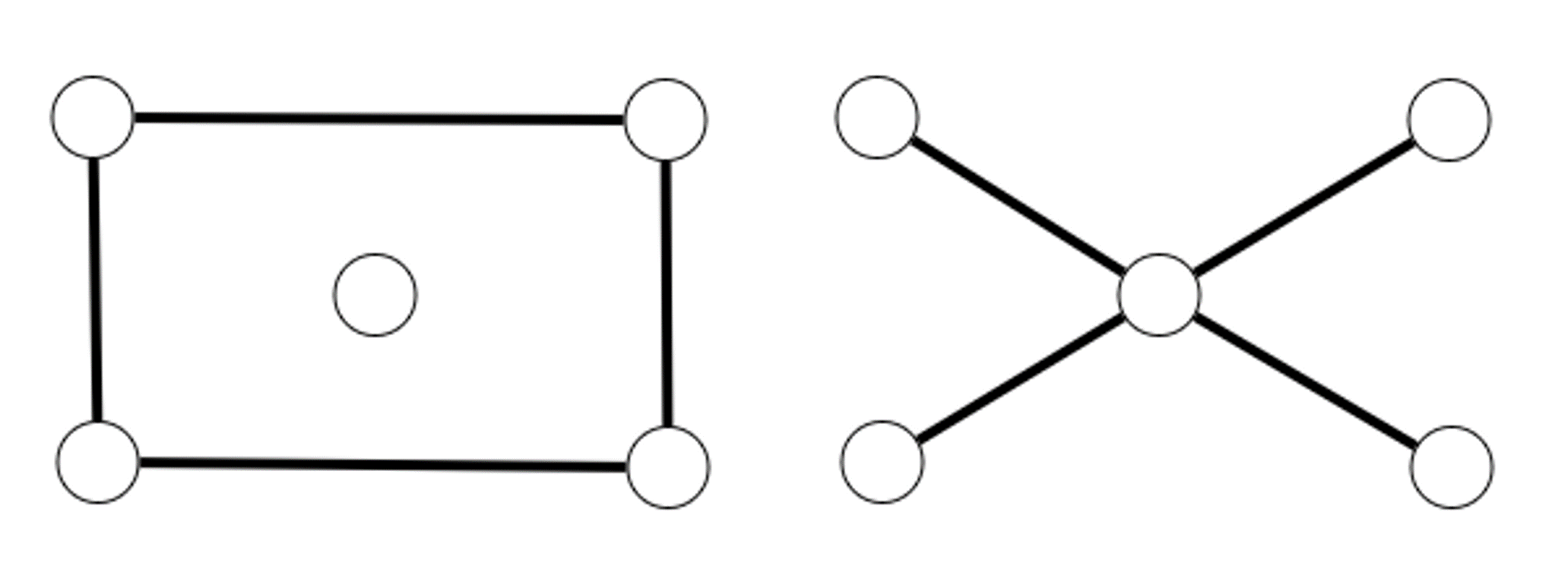
   Figure 1. The graphs $\operatorname{\mathsf{S}}_{4}=\operatorname{\mathsf{K}}_{1,4}$ and $\operatorname{\mathsf{C}}_{4}\cup\operatorname{\mathsf{K}}_{1}$ (i.e., a union of a 4-length cycle and an isolated vertex) are cospectral and nonisomorphic graphs ($\operatorname{\mathbf{A}}$-NICS graphs) on five vertices. These two graphs therefore cannot be determined by their adjacency matrix.

   Apart from these two $\operatorname{\mathbf{A}}$-NICS graphs, it can be verified by computer search that all of the other graphs on five vertices are $\operatorname{\mathbf{A}}$-DS.

   Theorem 3.11.

   [23] All the regular graphs with less than ten vertices are DS (and thus $\mathcal{X}$-DS for every $\mathcal{X}\subseteq\{\operatorname{\mathbf{A}},\operatorname{\mathbf{L}},\operatorname{\mathbf{Q}},\bf{\mathcal{L}}\}$).

   Example 3.12.

   [23] The following two regular graphs in Figure 2 are $\{\operatorname{\mathbf{A}},\operatorname{\mathbf{L}},\operatorname{\mathbf{Q}},\bf{\mathcal{L}}\}$-NICS.

   

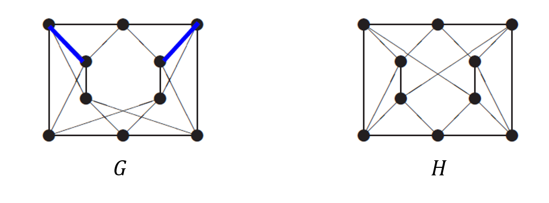
   Figure 2. $\{\operatorname{\mathbf{A}},\operatorname{\mathbf{L}},\operatorname{\mathbf{Q}},\bf{\mathcal{L}}\}$-NICS regular graphs with $10$ vertices.

   The regular graphs $\mathsf{G}$ and $\mathsf{H}$ in Figure 2 can be verified to be cospectral with the common characteristic polynomial

   $$P(x)=x^{10}-20x^{8}-16x^{7}+110x^{6}+136x^{5}-180x^{4}-320x^{3}+9x^{2}+200x+80.$$

   These graphs are also nonisomorphic because each of the two blue edges in $\mathsf{G}$ belongs to three triangles, whereas no such edge exists in $\mathsf{H}$. Furthermore, it is shown in Example 4.18 of [56] that each pair of the regular NICS graphs on 10 vertices, denoted by $\{\mathsf{G},\mathsf{H}\}$ and $\{\overline{\mathsf{G}},\overline{\mathsf{H}}\}$, exhibits distinct values of the Lovász $\vartheta$-functions, whereas the graphs $\mathsf{G}$, $\overline{\mathsf{G}}$, $\mathsf{H}$, and $\overline{\mathsf{H}}$ share identical independence numbers (3), clique numbers (3), and chromatic numbers (4). Furthermore, based on these two pairs of graphs, it is constructively shown in Theorem 4.19 of [56] that for every even integer $n\geq 14$, there exist connected, irregular, cospectral, and nonisomorphic graphs on $n$ vertices, being jointly cospectral with respect to their adjacency, Laplacian, signless Laplacian, and normalized Laplacian matrices, while also sharing identical independence, clique, and chromatic numbers, but being distinguished by their Lovász $\vartheta$-functions.

   Remark 3.13.

   In continuation to Example 3.12, it is worth noting that a closed-form expression for the Lovász $\vartheta$-functions of regular graphs, which are edge-transitive or strongly regular, have been derived in Theorem 9 of [46] and Proposition 1 of [55], respectively. In particular, it follows from Proposition 1 of [55] that strongly regular graphs with identical four parameters $(n,d,\lambda,\mu)$ are cospectral and they have identical Lovász $\vartheta$-numbers, although they need not be necessarily isomorphic. For such an explicit counterexample, the reader is referred to Remark 3 of [55].

   We next introduce friendship graphs to address their possible determination by their spectra with respect to several associated matrices.

   Definition 3.14.

   Let $p\in\mathbb{N}$. The friendship graph $\operatorname{\mathsf{F}}_{p}$, also known as the windmill graph, is a graph with $2p+1$ vertices, consisting of a single vertex (the central vertex) that is adjacent to all the other $2p$ vertices. Furthermore, every pair of these $2p$ vertices shares exactly one common neighbor, namely the central vertex (see Figure 3). This graph has $3p$ edges and $p$ triangles.

   The term friendship graph in Definition 3.14 originates from the Friendship Theorem [28]. This theorem states that if $\mathsf{G}$ is a finite graph where any two vertices share exactly one common neighbor, then there exists a vertex that is adjacent to all other vertices. In this context, the adjacency of vertices in the graph can be interpreted socially as a representation of friendship between the individuals represented by the vertices (assuming friendship is a mutual relationship). For a nice exposition of the proof of the Friendship Theorem, the interested reader is referred to Chapter 44 of [4].

   

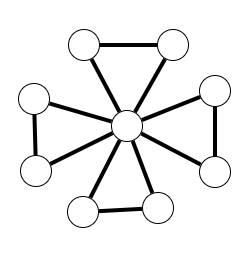
   Figure 3. The friendship graph $\operatorname{\mathsf{F}}_{4}$

   Theorem 3.15.

   The following graphs are DS:

   • The graphs $\operatorname{\mathsf{K}}_{n}$, $\operatorname{\mathsf{C}}_{n}$, $\operatorname{\mathsf{P}}_{n}$, $\operatorname{\mathsf{K}}_{m,m}$ and $\overline{\mathsf{\operatorname{\mathsf{K}}_{n}}}$ [23].

   • The disjoint union of $k$ path graph with no isolated vertices, the disjoint union of $k$ complete graphs with no isolated vertices and the disjoint union of $k$ cycles [23].

   • The friendship graph $\operatorname{\mathsf{F}}_{p}$ for $p\neq 16$ [19].

   Since the graphs $\operatorname{\mathsf{K}}_{n}$, $\overline{\mathsf{\operatorname{\mathsf{K}}_{n}}}$, $\operatorname{\mathsf{K}}_{m,m}$ and $\operatorname{\mathsf{C}}_{n}$ are regular, they are also $\mathcal{X}$-DS for every $\mathcal{X}\subseteq\{\operatorname{\mathbf{A}},\operatorname{\mathbf{L}},\operatorname{\mathbf{Q}},\bf{\mathcal{L}}\}$).

   3.3. Graphs determined by their spectra with respect to various matrices (X-DS graphs)

   Theorem 3.16.

   The following graphs are $\operatorname{\mathbf{L}}$-DS:

   • $\operatorname{\mathsf{P}}_{n},\operatorname{\mathsf{C}}_{n},\operatorname{\mathsf{K}}_{n},\operatorname{\mathsf{K}}_{m,m}$ and their complements [23].

   • The union of $k$ disjoint paths, $\operatorname{\mathsf{P}}_{n_{1}}+\operatorname{\mathsf{P}}_{n_{2}}+\ldots+\operatorname{\mathsf{P}}_{n_{k}}$ each having at least one edge [23].

   • The complete bipartite graph $\operatorname{\mathsf{K}}_{m,n}$ with $m,n\geq 2$ and $\frac{5}{3}n<m$ [7].

   • The star graph $\operatorname{\mathsf{S}}_{n}$ [51, 45].

   • The friendship graph $\operatorname{\mathsf{F}}_{p}$ [45].

   Remark 3.17.

   In general, a disjoint union of complete graphs is not determined by its Laplacian spectrum.

   Theorem 3.18.

   The following graphs are $\operatorname{\mathbf{Q}}$-DS:

   • The star $\operatorname{\mathsf{S}}_{n}$ for $n\neq 3$ [51].

   • The friendship graph $\operatorname{\mathsf{F}}_{k}$ [62].

   • $\mathsf{G}\vee\operatorname{\mathsf{K}}_{1}$ where $\mathsf{G}$ is a either a $1$-regular graph, an $(n-2)$-regular graph of order $n$ or a $2$-regular graph with at least $11$ vertices [10].

   • If $n\geq 21$ and $0\leq q\leq n-1$, then $\operatorname{\mathsf{K}}_{1}\vee(\operatorname{\mathsf{P}}_{q}\cup\,(n-q-1)\operatorname{\mathsf{K}}_{1})$ [64].

   • If $n\geq 21$ and $3\leq q\leq n-1$, then $\operatorname{\mathsf{K}}_{1}\vee(\operatorname{\mathsf{C}}_{q}\cup\,(n-q-1)\operatorname{\mathsf{K}}_{1})$ is $\operatorname{\mathbf{Q}}$-DS if and only if $q\neq 3$ [64].

   Theorem 3.19.

   [6] The friendship graph $\operatorname{\mathsf{F}}_{k}$ is ${\bf{\mathcal{L}}}$-DS.

   4. Special families of graphs

   This section introduces special families of structured graphs and it states conditions for their unique determination by their spectra.

   4.1. Stars and graphs of pyramids

   Definition 4.1.

   For every $k,n\in\mathbb{N}$ with $k<n$, define the graph $T_{n,k}=\operatorname{\mathsf{K}}_{k}\vee\,\overline{\operatorname{\mathsf{K}}_{n-k}}$. For $k=1$, the graph $T_{n,k}$ represents the star graph $\operatorname{\mathsf{S}}_{n}$. For $k=2$, it represents a graph comprising $n-2$ triangles sharing a common edge, referred to as a crown. For $n,k$ satisfying $1<k<n$, the graphs $T_{n,k}$ are referred to as graphs of pyramids [43].

   Theorem 4.2.

   [43] The graphs of pyramids are DS for every $1<k<n$.

   Theorem 4.3.

   [43] The star graph $\operatorname{\mathsf{S}}_{n}$ is DS if and only if $n-1$ is prime.

   To prove these theorems, a closed-form expression for the spectrum of $T_{n,k}$ is derived in [43], which also presents a generalized result. Subsequently, using Theorem 2.20, the number of edges and triangles in any graph cospectral with $T_{n,k}$ are calculated. Finally, Schur’s theorem (Theorem 2.2) and Cauchy’s interlacing theorem (Theorem 2.3) are applied in [43] to prove Theorems 4.2 and 4.3.

   4.2. Complete bipartite graphs

   By Theorem 4.3, the star graph $\operatorname{\mathsf{S}}_{n}=\operatorname{\mathsf{K}}_{1,n-1}$ is DS if and only if $n-1$ is prime. By Theorem 3.15, the regular complete bipartite graph $\operatorname{\mathsf{K}}_{m,m}$ is DS for every $m\in\mathbb{N}$. Here, we generalize these results and provide a characterization for the DS property of $\operatorname{\mathsf{K}}_{p,q}$ for every $p,q\in\mathbb{N}$.

   Theorem 4.4.

   [23] The spectrum of the complete bipartite graph $\operatorname{\mathsf{K}}_{p,q}$ is $\bigl{\{}-\sqrt{pq},[0]^{p+q-2},\sqrt{pq}\bigr{\}}$.

   This theorem can be proved by Theorem 2.2. An alternative simple proof is next presented.

   Proof.

   The adjacency matrix of $\operatorname{\mathsf{K}}_{p,q}$ is given by

   (4.1) $$\operatorname{\mathbf{A}}(\operatorname{\mathsf{K}}_{p,q})=\begin{pmatrix}\mathbf{0}_{p,p}&\operatorname{\mathbf{J}}_{p,q}\\ \operatorname{\mathbf{J}}_{q,p}&\mathbf{0}_{q,q}\end{pmatrix}\in\mathbb{R}^{(p+q)\times(p+q)}$$

   The rank of $\operatorname{\mathbf{A}}(\operatorname{\mathsf{K}}_{p,q})$ is equal to 2, so the multiplicity of $0$ as an eigenvalue is $p+q-2$. By Corollary 2.22, the two remaining eigenvalues are given by $\pm\lambda$ for some $\lambda\in\mathbb{R}$, since the eigenvalues sum to zero. Furthermore,

   (4.2) $$2\lambda^{2}=\sum_{i=1}^{p+q}\lambda_{i}^{2}=2\,|\operatorname{\mathsf{E}}(\operatorname{\mathsf{K}}_{p,q})|=2pq,$$

   so $\lambda=\sqrt{pq}$. ∎

   Definition 4.5.

   Let $p,q\in\mathbb{N}$.

   • The arithmetic mean of $p,q$ is given by $\text{AM}{(p,q)}=\tfrac{1}{2}(p+q)$.

   • The geometric mean of $p,q$ is given by $\text{GM}{(p,q)}=\sqrt{pq}$.

   Theorem 4.6 (AM-GM inequality).

   For every $p,q\in\mathbb{N}$, we have $\text{GM}{(p,q)}\leq\text{AM}{(p,q)}$ with equality if and only if $p=q$.

   Definition 4.7.

   Let $p,q\in\mathbb{N}$. The two-elements multiset $\{p,q\}$ is said to be an AM-minimizer if it attains the minimum arithmetic mean for their given geometric mean, i.e.,

   (4.3) $$\text{AM}{(p,q)} =\min\Bigl{\{}\text{AM}{(a,b)}:\;a,b\in\mathbb{N},\,\text{GM}{(a,b)}=\text{GM}{(p,q)}\Bigr{\}}$$

   (4.4) $$=\min\Bigl{\{}\tfrac{1}{2}(a+b):\;a,b\in\mathbb{N},\,ab=pq\Bigr{\}}.$$

   Example 4.8.

   The following are AM-minimizers:

   • $\{k,k\}$ for every $k\in\mathbb{N}$. By the AM-GM inequality, it is the only case where $\text{GM}{(p,q)}=\text{AM}{(p,q)}$.

   • $\{p,q\}$ where $p,q$ are prime numbers. In this case, the following family of multisets

     (4.5) $$\Bigl{\{}\{a,b\}:\,a,b\in\mathbb{N},\;\text{GM}{(a,b)}=\text{GM}{(p,q)}\Bigr{\}}$$

     only contains the two multisets $\{p,q\},\{pq,1\}$, and $p+q\leq pq<pq+1$ since $p,q\geq 2$.

   • $\{1,q\}$ where $q$ is a prime number.

   Theorem 4.9.

   The following holds for every $p,q\in\mathbb{N}$:

   1. Let $\mathsf{G}$ be a graph that is cospectral with $\operatorname{\mathsf{K}}_{p,q}$. Then, up to isomorphism, $G=\operatorname{\mathsf{K}}_{a,b}\cup\mathsf{H}$ (i.e., $\mathsf{G}$ is a disjoint union of the two graphs $\operatorname{\mathsf{K}}_{a,b}$ and $\mathsf{H}$), where $\mathsf{H}$ is an empty graph and $a,b\in\mathbb{N}$ satisfy $\text{GM}{(a,b)}=\text{GM}{(p,q)}$.

   2. The complete bipartite graph $\operatorname{\mathsf{K}}_{p,q}$ is DS if and only if $\{p,q\}$ is an AM-minimizer.

   Remark 4.10.

   Item 4b in Theorem 4.9 is equivalent to Corollary 3.1 in [48], for which an alternative proof is presented here.

   Proof.

   1. Let $\mathsf{G}$ be a graph cospectral with $\operatorname{\mathsf{K}}_{p,q}$. The number of edges in $\mathsf{G}$ equals the number of edges in $\operatorname{\mathsf{K}}_{p,q}$, which is $pq$. As $\operatorname{\mathsf{K}}_{p,q}$ is bipartite, so is $\mathsf{G}$. Since $\operatorname{\mathbf{A}}(\mathsf{G})$ is of rank $2$, and $\operatorname{\mathbf{A}}(\operatorname{\mathsf{P}}_{3})$ has rank $3$, it follows from the Cauchy’s Interlacing Theorem (Theorem 2.3) that $\operatorname{\mathsf{P}}_{3}$ is not an induced subgraph of $\mathsf{G}$.
      It is claimed that $\mathsf{G}$ has a single nonempty connected component. Suppose to the contrary that $\mathsf{G}$ has (at least) two nonempty connected components $\mathsf{H}_{1},\mathsf{H}_{2}$. For $i\in\{1,2\}$, since $\mathsf{H}_{i}$ is a non-empty graph, $\operatorname{\mathbf{A}}(\mathsf{H}_{i})$ has at least one eigenvalue $\lambda\neq 0$. Since $\mathsf{G}$ is a simple graph, the sum of the eigenvalues of $\operatorname{\mathbf{A}}(\mathsf{H}_{i})$ is $\text{Tr}{(\operatorname{\mathbf{A}}(\mathsf{H}_{i}))}=0$, so $\mathsf{H}_{i}$ has at least one positive eigenvalue. Thus, the induced subgraph $\mathsf{H}_{1}\cup\mathsf{H}_{2}$ has at least two positive eigenvalues, while $\mathsf{G}$ has only one positive eigenvalue, contradicting Cauchy’s Interlacing Theorem.

   Hence, $\mathsf{G}$ can be decomposed as $\mathsf{G}=\operatorname{\mathsf{K}}_{a,b}\cup\,\mathsf{H}$ where $\mathsf{H}$ is an empty graph. Since $\mathsf{G}$ and $\operatorname{\mathsf{K}}_{p,q}$ have the same number of edges, $pq=ab$, so $\text{GM}{(p,q)}=\text{GM}{(a,b)}$.

5. First, we will show that if $\{p,q\}$ is not an AM-minimizer, then the graph $\operatorname{\mathsf{K}}_{p,q}$ is not $\operatorname{\mathbf{A}}$-DS. This is done by finding a nonisomorphic graph to $\operatorname{\mathsf{K}}_{p,q}$ that is $\operatorname{\mathbf{A}}$-cospectral with it. By assumption, since $\{p,q\}$ is not an AM-minimizer, there exist $a,b\in\mathbb{N}$ satisfying $\text{GM}{(a,b)}=\text{GM}{(p,q)}$ and $a+b<p+q$. Define the graph $\mathsf{G}=\operatorname{\mathsf{K}}_{a,b}\vee\,\overline{\operatorname{\mathsf{K}}_{r}}$ where $r=p+q-a-b$. Observe that $r\in\mathbb{N}$. The $\operatorname{\mathbf{A}}$-spectrum of both of these graphs is given by

   (4.6) $$\sigma_{\operatorname{\mathbf{A}}}(\mathsf{G})=\sigma_{\operatorname{\mathbf{A}}}(\operatorname{\mathsf{K}}_{p,q})=\bigl{\{}-\sqrt{pq},[0]^{pq-2},\sqrt{pq}\bigr{\}},$$

   so these two graphs are nonisomorphic and cospectral, which means that $\mathsf{G}$ is not $\operatorname{\mathbf{A}}$-DS.
   We next prove that if $\{p,q\}$ is an AM-minimizer, then $\operatorname{\mathsf{K}}_{p,q}$ is $\operatorname{\mathbf{A}}$-DS. Let $\mathsf{G}$ be a that is cospectral graph with $\operatorname{\mathsf{K}}_{p,q}$, then from the first part of this theorem, $\mathsf{G}=\operatorname{\mathsf{K}}_{a,b}\cup\,\mathsf{H}$ where $\text{GM}{(a,b)}=\text{GM}{(p,q)}$ and $\mathsf{H}$ is an empty graph. Hence, $\text{AM}{(a,b)}=\tfrac{1}{2}(a+b)\leq\tfrac{1}{2}(p+q)=\text{AM}{(p,q)}$. Since $\{p,q\}$ is by assumption an AM-minimizer, also $\text{AM}{(a,b)}\geq\text{AM}{(p,q)}$, so equality holds. Both equalities $\text{GM}{(a,b)}=\text{GM}{(p,q)}$ and $\text{AM}{(a,b)}=\text{AM}{(p,q)}$ can be satisfied simultaneously if and only if $\{a,b\}=\{p,q\}$, so $r=p+q-a-b=0$ and $\mathsf{G}=\operatorname{\mathsf{K}}_{p,q}$.

   ∎

   Corollary 4.11.

   Almost all of the complete bipartite graphs are not DS. More specifically, for every $n\in\mathbb{N}$, there exists a single complete bipartite graph on $n$ vertices that is DS.

   Proof.

   Let $n\in\mathbb{N}$. By the fundamental theorem of arithmetic, there is a unique decomposition $n=\prod_{i=1}^{k}p_{i}$ where $k\in\mathbb{N}$ and $\{p_{i}\}$ are prime numbers for every $1\leq i\leq k$. Consider the family of multisets

   (4.7) $$\mathcal{D}=\Bigl{\{}\{a,b\}:a,b\in\mathbb{N},\text{GM}{(a,b)}=\sqrt{n}\Bigr{\}}.$$

   This family has $2^{k}$ members, since every prime factor $p_{i}$ of $n$ should be in the prime decomposition of $a$ or $b$. Since the minimization of $\text{AM}{(a,b)}$ under the equality constraint $\text{GM}{(a,b)}=\sqrt{n}$ forms a convex optimization problem, only one of the multisets in the family $\mathcal{D}$ is an AM-minimizer. Thus, if $n=\prod_{i=1}^{k}p_{i}$, then the number of complete bipartite graphs of $n$ vertices is $O(2^{k})$, and (by Item 4b of Theorem 4.9) only one of them is DS. ∎

   4.3. Turán graphs

   Definition 4.12.

   Let $n_{1},\ldots,n_{k}$ be natural numbers. Define the complete $k$-partite graph

   (4.8) $$\operatorname{\mathsf{K}}_{n_{1},\ldots,n_{k}}=\bigvee_{i=1}^{k}\overline{\operatorname{\mathsf{K}}_{n_{i}}}.$$

   A graph is multipartite if it is $k$-partite for some $k\geq 2$.

   Definition 4.13.

   Let $2\leq k\leq n$. The Turán graph $T(n,k)$ (not to be confused with the graph of pyramids $T_{n,k}$) is formed by partitioning a set of $n$ vertices into $k$ subsets, with sizes as equal as possible, and then every two vertices are adjacent in that graph if and only if they belong to different subsets. It is therefore expressed as the complete $k$-partite graph $K_{n_{1},\dots,n_{k}}$, where $|n_{i}-n_{j}|\leq 1$ for all $i,j\in[k]$ with $i\neq j$. Let $q$ and $s$ be the quotient and remainder, respectively, of dividing $n$ by $k$ (i.e., $n=qk+s$, $s\in\{0,1,\ldots,k-1\}$), and let $n_{1}\leq\ldots\leq n_{k}$. Then,

   (4.9) $$n_{i}=\begin{cases}q,&1\leq i\leq k-s,\\ q+1,&k-s+1\leq i\leq k.\end{cases}$$

   By construction, the graph $T(n,k)$ has a clique of order $k$ (any subset of vertices with a single representative from each of the $k$ subsets is a clique of order $k$), but it cannot have a clique of order $k+1$ (since vertices from the same subset are nonadjacent). Note also that, by (4.9), the Turán graph $T(n,k)$ is a $q$-regular graph if and only if $n$ is divisible by $k$, and then $q=\frac{n}{k}$.

   Definition 4.14.

   Let $q,k\in\mathbb{N}$. Define the regular complete multipartite graph, $\mathrm{K}_{q}^{k}:=\overset{k}{\underset{i=1}{\bigvee}}\overline{\operatorname{\mathsf{K}}_{q}}$, to be the $k$-partite graph with $q$ vertices in each part. Observe that $\mathrm{K}_{q}^{k}=T(kq,k)$.

   Let $\mathsf{G}$ be a simple graph on $n$ vertices that does not contain a clique of order greater than a fixed number $k\in\mathbb{N}$. Turán investigated a fundamental problem in extremal graph theory of determining the maximum number of edges that $\mathsf{G}$ can have [61].

   Theorem 4.15 (Turán’s Graph Theorem).

   Let $\mathsf{G}$ be a graph on $n$ vertices with a clique of order at most $k$ for some $k\in\mathbb{N}$. Then,

   (4.10) $$|\operatorname{\mathsf{E}}(\mathsf{G})| \leq|\operatorname{\mathsf{E}}(T(n,k))|$$

   (4.11) $$=\biggl{(}1-\frac{1}{k}\biggr{)}\,\frac{n^{2}-s^{2}}{2}+\binom{s}{2},\quad s\triangleq n-k\bigg{\lfloor}\frac{n}{k}\bigg{\rfloor}.$$

   For a nice exposition of five different proofs of Turán’s Graph Theorem, the interested reader is referred to Chapter 41 of [4].

   Corollary 4.16.

   Let $k\in\mathbb{N}$, and let $\mathsf{G}$ be a graph on $n$ vertices where $\omega(\mathsf{G})\leq k$ and $|\operatorname{\mathsf{E}}(\mathsf{G})|=|\operatorname{\mathsf{E}}(T(n,k))|$. Let $\mathsf{G}_{1}$ be the graph obtained by adding an arbitrary edge to $\mathsf{G}$. Then $\omega(\mathsf{G}_{1})>k$.

   4.3.1. The spectrum of the Turán graph

   Theorem 4.17.

   [29] Let $k\in\mathbb{N}$, and let $n_{1}\leq n_{2}\leq\ldots\leq n_{k}$ be natural numbers. Let $\mathsf{G}=\operatorname{\mathsf{K}}_{n_{1},n_{2},\dots,n_{k}}$ be a complete multipartite graph on $n=n_{1}+\ldots n_{k}$ vertices. Then,

   • $\mathsf{G}$ has one positive eigenvalue, i.e., $\lambda_{1}(\mathsf{G})>0$ and $\lambda_{2}(\mathsf{G})\leq 0$.

   • $\mathsf{G}$ has $0$ as an eigenvalue with multiplicity $n-k$.

   • $\mathsf{G}$ has $k-1$ negative eigenvalues, and

     (4.12) $$n_{1}\leq-\lambda_{n-k+2}(\mathsf{G})\leq n_{2}\leq-\lambda_{n-k+3}(\mathsf{G})\leq n_{3}\leq\ldots\leq n_{k-1}\leq-\lambda_{n}(\mathsf{G})\leq n_{k}.$$

   Corollary 4.18.

   The spectrum of the regular complete $k$-partite graph $\operatorname{\mathsf{K}}_{q,\ldots,q}\triangleq\operatorname{\mathsf{K}}_{q}^{k}$ is given by

   (4.13) $$\sigma_{\operatorname{\mathbf{A}}}(\operatorname{\mathsf{K}}_{q}^{k})=\Bigl{\{}[-q]^{k-1},[0]^{(q-1)k},q(k-1)\Bigr{\}}.$$

   Proof.

   This readily follows from Theorem 4.17 by setting $n_{1}=\ldots=n_{k}=q$. ∎

   Lemma 4.19.

   [11] Let $\mathsf{G}_{i}$ be $r_{i}$-regular graphs on $n_{i}$ vertices for $i\in\{1,2\}$, with the adjacency spectrum $\sigma_{\operatorname{\mathbf{A}}}(\mathsf{G}_{1})=(r_{1}=\mu_{1}\geq\mu_{2}\geq...\geq\mu_{n})$ and $\sigma_{A}(\mathsf{G}_{2})=(r_{2}=\nu_{1}\geq\nu_{2}\geq...\geq\nu_{n})$. The $\operatorname{\mathbf{A}}$-spectrum of $\mathsf{G}_{1}\vee\mathsf{G}_{2}$ is given by

   (4.14) $$\sigma_{\operatorname{\mathbf{A}}}(\mathsf{G}_{1}\vee\mathsf{G}_{2})=\{\mu_{i}\}_{i=2}^{n_{1}}\cup\{\nu_{i}\}_{i=2}^{n_{2}}\cup\left\{\frac{r_{1}+r_{2}\pm\sqrt{(r_{1}-r_{2})^{2}+4n_{1}n_{2}}}{2}\right\}.$$

   Theorem 4.20.

   Let $q,s\in\mathbb{N}$ such that $n=kq+s$ and $0\leq s\leq k-1.$ The following holds with respect to the $\operatorname{\mathbf{A}}$-spectrum of $T(n,k)$:

   1. If $1\leq s\leq k-1$, then the $\operatorname{\mathbf{A}}$-spectrum of the irregular Turán graph $T(n,k)$ is given by

      $$\sigma_{\operatorname{\mathbf{A}}}(T(n,k))= \biggl{\{}[-q-1]^{s-1},[-q]^{k-s-1},[0]^{n-k}\biggr{\}}$$

      (4.15) $$\cup\Biggl{\{}\tfrac{1}{2}\biggl{[}n-2q-1\pm\sqrt{\Bigl{(}n-2(q+1)s+1\Bigr{)}^{2}+4q(q+1)s(k-s)}\biggr{]}\Biggr{\}}.$$

   2. If $s=0$, then $q=\frac{n}{k}$, and the $\operatorname{\mathbf{A}}$-spectrum of the regular Turán graph $T(n,k)$ is given by

      (4.16) $$\sigma_{\operatorname{\mathbf{A}}}(T(n,k))= \Bigl{\{}[-q]^{k-1},[0]^{n-k},(k-1)q\Bigr{\}}.$$

   Proof.

   Let $1\leq s\leq k-1$, and we next derive the $\operatorname{\mathbf{A}}$-spectrum of an irregular Turán graph $T(n,k)$ in Item 4a (i.e., its spectrum if $n$ is not divisible by $k$ since $s\neq 0$). By Corollary 4.18, the spectra of the regular graphs $\operatorname{\mathsf{K}}_{q}^{k-s}$ and $\operatorname{\mathsf{K}}_{q+1}^{s}$ is

   (4.17) $$\sigma_{\operatorname{\mathbf{A}}}(\operatorname{\mathsf{K}}_{q}^{k-s})=\left\{[-q]^{k-s-1},[0]^{(q-1)(k-s)},q(k-s-1)\right\},$$

   (4.18) $$\sigma_{\operatorname{\mathbf{A}}}(\operatorname{\mathsf{K}}_{q+1}^{s})=\left\{[-q-1]^{s-1},[0]^{qs},(q+1)(s-1)\right\}.$$

   The $(k-s)$-partite graph $\operatorname{\mathsf{K}}_{q}^{k-s}$ is $r_{1}$-regular with $r_{1}=q(k-s-1)$, the $s$-partite graph $\operatorname{\mathsf{K}}_{q+1}^{s}$ is $r_{2}$-regular with $r_{2}=(q+1)(s-1)$, and by Definition 4.13, we have $T(n,k)=\operatorname{\mathsf{K}}_{q}^{k-s}\vee\operatorname{\mathsf{K}}_{q+1}^{s}$. Hence, by Lemma 4.19, the adjacency spectrum of $T(n,k)$ is given by

   $$\sigma_{\operatorname{\mathbf{A}}}(T(n,k)) =\sigma_{\operatorname{\mathbf{A}}}(\operatorname{\mathsf{K}}_{q}^{k-s}\vee\operatorname{\mathsf{K}}_{q+1}^{s})$$

   (4.19) $$=\mathcal{S}_{1}\cup\mathcal{S}_{2}\cup\mathcal{S}_{3},$$

   where

   (4.20) $$\mathcal{S}_{1} =\Bigl{\{}[-q]^{k-s-1},[0]^{(q-1)(k-s)}\Bigr{\}},$$

   (4.21) $$\mathcal{S}_{2} =\Bigl{\{}[-q-1]^{s-1},[0]^{qs}\Bigr{\}},$$

   $$\mathcal{S}_{3} =\biggl{\{}\frac{r_{1}+r_{2}\pm\sqrt{(r_{1}-r_{2})^{2}+4n_{1}n_{2}}}{2}\biggr{\}}$$

   (4.22) $$=\Biggl{\{}\tfrac{1}{2}\biggl{[}n-2q-1\pm\sqrt{\Bigl{(}n-2(q+1)s+1\Bigr{)}^{2}+4q(q+1)s(k-s)}\biggr{]}\Biggr{\}},$$

   where the last equality holds since, by the equality $n=kq+s$ and the above expressions of $r_{1}$ and $r_{2}$, it can be readily verified that $r_{1}+r_{2}=n-2q-1$ and $r_{1}-r_{2}=n-2(q+1)s+1$. Finally, combining (4.19)–(4.22) gives the $\operatorname{\mathbf{A}}$-spectrum in (4.15) of an irregular Turán graph $T(n,k)$.

   We next prove Item 4b, referring to a regular Turán graph $T(n,k)$ (i.e., $k|n$ or equivalently, $s=0$). In that case, we have $T(n,k)=\operatorname{\mathsf{K}}_{q}^{k}$ where $q=\frac{n}{k}$, so the $\operatorname{\mathbf{A}}$-spectrum in (4.16) holds by Corollary 4.18. ∎

   Remark 4.21.

   In light of Theorem 4.20, if $k\geq 2$, then the number of negative eigenvalues (including multiplicities) of the adjacency matrix of the Turán graph $T(n,k)$ is $k-1$ if the graph is regular (i.e., if $k|n$), and it is $k-2$ otherwise (i.e., if the graph is irregular). If $k=1$, which corresponds to an empty graph (having no edges), then all eigenvalues are zeros (having no negative eigenvalues). Furthermore, the adjacency matrix of $T(n,k)$ always has a single positive eigenvalue, which is of multiplicity 1 irrespectively of the values of $n$ and $k$. We rely on these properties later in this paper (see Section 4.3.2).

   Example 4.22.

   By Theorem 4.20, let us calculate the $\operatorname{\mathbf{A}}$-spectrum of the Turán graph $T(17,7)$, and verify it numerically with the SageMath software. Having $n=17$ and $k=7$ gives $q=2$ and $s=3$, which by Theorem 4.20 implies that

   (4.23) $$\sigma_{\operatorname{\mathbf{A}}}\bigl{(}T(17,7)\bigr{)}=\Bigl{\{}[-3]^{2},[-2]^{3},[0]^{10},\,6(1+\sqrt{2}),\,6(1-\sqrt{2})\Bigr{\}}.$$

   That has been numerically verified by programming in the SageMath software.

   4.3.2. Turán graphs are DS

   The main result of this subsection establishes that all Turán graphs are determined by their $\operatorname{\mathbf{A}}$-spectrum. This result is equivalent to Theorem 3.3 in [48], while also presenting an alternative proof that offers additional insights.

   Theorem 4.23.

   The Turán graph $T(n,k)$ is $\operatorname{\mathbf{A}}$-DS.

   In order to prove Theorem 4.23, we first introduce an auxiliary result from [59], followed by several other lemmata.

   Theorem 4.24.

   [59, Theorem 1] Let $\mathsf{G}$ be a graph. Then, the following statements are equivalent:

   • $\mathsf{G}$ has exactly one positive eigenvalue.

   • $\mathsf{G}=\mathsf{H}\cup\overline{\mathsf{\operatorname{\mathsf{K}}_{m}}}$ for some $m$, where $\mathsf{H}$ is a nonempty complete multipartite graph. In other words, the non-isolated vertices of $\mathsf{G}$ form a complete multipartite graph.

   Proof of Theorem 4.23.

   Let $\mathsf{G}$ be a graph that is $\operatorname{\mathbf{A}}$-cospectral with $T(n,k)$. Denote $n=qk+s$ for $s,q\in\mathbb{N}$ such that $0\leq s<k$.

   Lemma 4.25.

   The graph $\mathsf{G}$ doesn’t have a clique of order $k+1$.

   Proof.

   Suppose to the contrary that the graph $\mathsf{G}$ has a clique of order $k+1$, which means that $\operatorname{\mathsf{K}}_{k+1}$ is an induced subgraph of $\mathsf{G}$. The complete graph $\operatorname{\mathsf{K}}_{k+1}$ has $k$ negative eigenvalues ($-1$ with a multiplicity of $k$). On the other hand, $\mathsf{G}$ has at most $k-1$ negative eigenvalues, $n-k$ zero eigenvalues, and exactly one positive eigenvalue; indeed, this follows from Theorem 4.20 (see Remark 4.21), and since $\mathsf{G}$ and $T(n,k)$ are $\operatorname{\mathbf{A}}$-cospectral graphs. Hence, by Cauchy’s Interlacing Theorem, every induced subgraph of $\mathsf{G}$ on $k+1$ vertices has at most $k-1$ negative eigenvalues (i.e., those eigenvalues interlaced between the negative and zero eigenvalues of $\mathsf{G}$ that are placed at distance $k+1$ apart in a sorted list of the eigenvalues of $\mathsf{G}$ in decreasing order). This contradicts our assumption on the existence of a clique of $k+1$ vertices because of the $k$ negative eigenvalues of $\operatorname{\mathsf{K}}_{k+1}$. ∎

   Lemma 4.26.

   The graph $\mathsf{G}$ is a complete multipartite graph.

   Proof.

   Since $\mathsf{G}$ has exactly one positive eigenvalue, which is of multiplicity one, we get from Theorem 4.24 that $\mathsf{G}=\mathsf{H}\cup\overline{\mathsf{\operatorname{\mathsf{K}}_{\ell}}}$ for some $\ell\in\mathbb{N}$, where $\mathsf{H}$ is a nonempty multipartite graph. We next show that $\ell=0$. Suppose to the contrary that $\ell\geq 1$, and let $v$ be an isolated vertex of $\overline{\mathsf{\operatorname{\mathsf{K}}_{\ell}}}$. Since $\mathsf{H}$ is a nonempty graph, there exists a vertex $u\in\operatorname{\mathsf{V}}(\mathsf{H})$. Let $\mathsf{G}_{1}$ be the graph obtained from $\mathsf{G}$ by adding the single edge $\{v,u\}$. By Lemma 4.25, $\mathsf{G}$ does not have a clique of order $k+1$. Hence, $\mathsf{G}_{1}$ does not have a clique of order $k+1$ either, contradicting Corollary 4.16. Hence, $\mathsf{G}=\mathsf{H}$. ∎

   Lemma 4.27.

   The graph $\mathsf{G}$ is a complete $k$-partite graph.

   Proof.

   By Lemma 4.26, $\mathsf{G}$ is a complete multipartite graph. Let $r$ be the number of partite subsets in the vertex set $\operatorname{\mathsf{V}}(\mathsf{G})$. We show that $r=k$, which then gives that $\mathsf{G}$ is a complete $k$-partite graph. By Lemma 4.25, $\mathsf{G}$ doesn’t have a clique of order $k+1$. Hence, $r\leq k$. Suppose to the contrary that $r<k$. Since $\mathsf{G}$ is a complete $r$-partite graph, the largest order of a clique in $\mathsf{G}$ is $r$. Let $\mathsf{G}_{1}$ be a graph obtained from $\mathsf{G}$ by adding an edge between two vertices within the same partite subset. The graph $\mathsf{G}_{1}$ becomes an $(r+1)$-partite graph. Consequently, the maximum order of a clique in $\mathsf{G}_{1}$ is at most $r+1\leq k$. The graph $\mathsf{G}_{1}$ has exactly one more edge than $\mathsf{G}$. Since $\mathsf{G}$ is $\operatorname{\mathbf{A}}$-cospectral to $T(n,k)$, it has the same number of edges as in $T(n,k)$. Hence, $\mathsf{G}_{1}$ contains more edges than $T(n,k)$, while also lacking a clique of order $k+1$. This contradicts Corollary 4.16, so we conclude that $r=k$. ∎

   Let $n_{1},n_{2},\dots,n_{k}\in\mathbb{N}$ be the number of vertices in each partite subset of the complete $k$-partite graph $\mathsf{G}$, i.e., $\mathsf{G}=\operatorname{\mathsf{K}}_{n_{1},n_{2},\dots,n_{k}}$. Then, the next two lemmata subsequently hold.

   Lemma 4.28.

   For all $i\in[k]$, $n_{i}\leq q+1$ .

   Proof.

   Suppose to the contrary that there exists a partite subset in the complete $k$-partite graph $\mathsf{G}$ with more than $q+1$ vertices. Let $\mathcal{P}_{1}$ be such a partite subset, and suppose without loss of generality that $n_{1}=|\mathcal{P}_{1}|\geq q+1$. By the pigeonhole principle, there exists a partite subset of $\mathsf{G}$ with at most $q$ vertices (since $\sum_{i\in[k]}n_{i}=n=kq+s$, where $0\leq s\leq k-1$). Let $\mathcal{P}_{2}$ be such a partite subset of $\mathsf{G}$, and suppose without loss of generality that $n_{2}=|\mathcal{P}_{2}|\leq q$. Let $\mathsf{G}_{1}$ be the graph obtained from $\mathsf{G}$ by removing a vertex $v\in\mathcal{P}_{1}$, adding a new vertex $u$ to $\mathcal{P}_{2}$, and connecting $u$ to all the vertices outside its partite subset. The new graph $\mathsf{G}_{1}$ is also $k$-partite, so it does not contain a clique of order greater than $k$. Furthermore, by construction, $\mathsf{G}_{1}$ has more edges than $\mathsf{G}$, so

   (4.24) $$\bigl{|}\operatorname{\mathsf{E}}(\mathsf{G}_{1})\bigr{|}>\bigl{|}\operatorname{\mathsf{E}}(\mathsf{G})\bigr{|}=\bigl{|}\operatorname{\mathsf{E}}(T(n,k))\bigr{|}.$$

   Hence, $\mathsf{G}_{1}$ is a graph with no clique of order greater than $k$, and it has more edges than $T(n,k)$. That contradicts Theorem 4.15, so $\{n_{i}\}_{i=1}^{k}$ cannot include any element that is larger than $q+1$. ∎

   Lemma 4.29.

   For all $i\in[k]$, $n_{i}\geq q$.

   Proof.

   The proof of this lemma is analogous to the proof of Lemma 4.28. Suppose to the contrary that there exists a partite subset of $\mathsf{G}$ with less than $q$ vertices. Let $\mathcal{P}_{1}$ be such a partite subset, so $p_{1}\triangleq\bigl{|}\mathcal{P}_{1}\bigr{|}<q$. By the pigeonhole principle, there exists a partition with at least $q+1$ vertices. Let $\mathcal{P}_{2}$ be such a partite subset set, whose number of vertices is denoted by $p_{2}\triangleq|\mathcal{P}_{2}|\geq q+1$. Let $\mathsf{G}_{1}$ be the graph obtained by removing a vertex $v\in\mathcal{P}_{2}$, adding a new vertex $u$ to $\mathcal{P}_{1}$, and connecting the vertex $u$ to all the vertices outside its partite subset. $\mathsf{G}_{1}$ is $k$-partite, so it does not contain a clique of order greater than $k$, and $\mathsf{G}_{1}$ has more edges than $\mathsf{G}$ so (4.24) holds. Hence, $\mathsf{G}_{1}$ is a graph with no clique of order greater than $k$, and it has more edges than $T(n,k)$. That contradicts Theorem 4.15, so $\{n_{i}\}_{i=1}^{k}$ cannot include any element that is smaller than $q$. ∎

   By Lemmata 4.28 and 4.29, we conclude that $n_{i}\in\{q,q+1\}$ for every $1\leq i\leq k-1$. Let $\alpha$ be the number of partite subsets of $q$ vertices and $\beta$ be the number of partite subsets of $q+1$ vertices. Since $\mathsf{G}$ has $n$ vertices, where $\sum n_{i}=n$, it follows that $q\alpha+(q+1)\beta=n$. Moreover, $\mathsf{G}$ is $k$-partite, so it follows that $\alpha+\beta=k$. This gives the linear system of equations

   (4.25) $$\begin{pmatrix}q&q+1\\ 1&1\end{pmatrix}\begin{pmatrix}\alpha\\ \beta\end{pmatrix}=\begin{pmatrix}n\\ k\end{pmatrix},$$

   which has the single solution

   (4.26) $$\alpha=k-s,\quad\beta=n-qk=s.$$

   Hence, $\mathsf{G}=T(n,k)$, which completes the proof of Theorem 4.23. ∎

   Remark 4.30.

   The proof of Theorem 4.23 is an alternative proof of Theorem 3.3 in [48]. While both proofs rely on Theorem 4.24, which is Theorem 1 of [59], our proof relies on the adjacency spectral characterization in Theorem 4.20, noteworthy in its own right, and further builds upon a sequence of results presented in Lemmata 4.25–4.29. On the other hand, the proof of Theorem 3.3 in [48] relies on Theorem 4.24, but then deviates substantially from our proof (see Lemmata 2.4 and 2.5 in [48] and Theorem 3.1 in [48], serving to prove Theorem 4.23).

   4.4. Nice graphs

   The family referred to as ”nice graphs” has been recently introduced in [42].

   Definition 4.31.

   • A graph $\mathsf{G}$ is sunlike if it is connected, and can be obtained from a cycle $\mathrm{C}$ by adding some vertices and connecting each of them to some vertex in $\mathrm{C}$.

   • Let $l,k\in\mathbb{N}$. A sunlike graph $\mathsf{G}$ is $(l,k)$-nice if it can be obtained by a cycle $\operatorname{\mathsf{C}}_{\ell}$ and

     • There is a single vertex $v_{1}\in\operatorname{\mathsf{V}}(\operatorname{\mathsf{C}}_{\ell})$ of degree $3$.

     • There are $k$ vertices $u_{1},\ldots,u_{k}\in\operatorname{\mathsf{V}}(\operatorname{\mathsf{C}}_{\ell})$ of degree $4$. Let $\mathcal{U}=\{u_{1},\ldots,u_{k}\}$.

     • By starting a walk on $\operatorname{\mathsf{C}}_{\ell}$ from $v_{1}$ at some orientation, then after 4 or 6 steps we get to a vertex $u_{1}\in\mathcal{U}$. Then, after another $4$ or $6$ steps from $u_{1}$ we get to $u_{2}\in\mathcal{U}$, and so on until we get to the vertex $u_{k}\in\mathcal{U}$.

   In order to present the next result from [42], we first introduce line graphs.

   Definition 4.32.

   The line graph of a graph $\mathsf{G}$, denoted by $\ell(\mathsf{G})$, is a graph whose vertices are the edges in $\mathsf{G}$, and two vertices are adjacent in $\ell(\mathsf{G})$ if the corresponding edges are incident in $\mathsf{G}$.

   Theorem 4.33.

   [42] Let $l,k\in\mathbb{N}$ such that $l\equiv 2\,(\text{mod }4)$. Let $\mathsf{G}$ be an $(l,k)$-nice graph. If the order of $\mathsf{G}$ is a prime number greater than some $n_{0}\in\mathbb{N}$, then the line graph $\ell(\mathsf{G})$ is DS.

   A more general class of graphs is introduced in [42], where it is shown that for every sufficiently large $n\in\mathbb{N}$, the number of nonisomorphic $n$-vertex graphs in that class that are determined by their $\operatorname{\mathbf{A}}$-spectrum is at least $e^{cn}$ for some positive constant $c$ (see [42, Theorem 1.4]). This recent result represents a significant advancement in the study of Haemers’ conjecture because the lower bounds on the number of nonisomorphic $n$-vertex graphs that are determined by their spectrum were all of the form of $e^{c\sqrt{n}}$, for some positive constant $c$. As noted in [42], the first form of such a lower bound was derived by van Dam and Haemers [24, Proposition 6], who proved that a graph $\mathsf{G}$ is DS whenever every connected component of $\mathsf{G}$ is a complete subgraph, leading to a lower bound that is approximately of the form $e^{c\sqrt{n}}$ with $c=\sqrt{\tfrac{2}{3}}\,\pi$. Therefore, the transition to a lower bound in [42] that scales exponentially with $n$, rather than with $\sqrt{n}$, is both remarkable and noteworthy.

   4.5. Friendship graphs and their generalization

   The next theorem considers whether friendship graphs (see Definition 3.14) can be uniquely determined by the spectra of four of their associated matrices.

   Theorem 4.34.

   • The friendship graph $\operatorname{\mathsf{F}}_{p}$ is DS if and only if $p\neq 16$ (i.e., the friendship graph is DS unless it has 16 triangles [19]).

   • The friendship graph $\operatorname{\mathsf{F}}_{p}$ is $\operatorname{\mathbf{L}}$-DS [44].

   • The friendship graph $\operatorname{\mathsf{F}}_{p}$ is $\operatorname{\mathbf{Q}}$-DS [62].

   • The friendship graph $\operatorname{\mathsf{F}}_{p}$ is ${\bf{\mathcal{L}}}$-DS [6].

   The friendship graph $\operatorname{\mathsf{F}}_{p}$, where $p\in\mathbb{N}$, can be expressed in the form $\operatorname{\mathsf{F}}_{p}=\operatorname{\mathsf{K}}_{1}\vee(p\operatorname{\mathsf{K}}_{2})$ (see Figure 3). The last observation follows from a property of a generalized friendship graph, which is defined as follows.

   Definition 4.35.

   Let $p,q\in\mathbb{N}$. The generalized friendship graph is given by $\operatorname{\mathsf{F}}_{p,q}=\operatorname{\mathsf{K}}_{1}\vee(p\operatorname{\mathsf{K}}_{q})$. Note that $\operatorname{\mathsf{F}}_{p,2}=\operatorname{\mathsf{F}}_{p}$.

   The following theorem addresses the conditions under which generalized friendship graphs can be uniquely determined by the spectra of their normalized Laplacian matrix.

   Theorem 4.36.

   The generalized friendship graph $\operatorname{\mathsf{F}}_{p,q}$ is ${\bf{\mathcal{L}}}$-DS if and only if $q\geq 2$, or $q=1$ and $p=2$ [6].

   Corollary 4.37.

   The friendship graph $\operatorname{\mathsf{F}}_{p}$ is ${\bf{\mathcal{L}}}$-DS [6].

   5. Graph operations for the construction of cospectral graphs

   This section presents such graph operations, focusing on unitary and binary transformations that enable the systematic construction of cospectral graphs. These operations are designed to preserve the spectral properties of the original graph while potentially altering its structure, thereby producing non-isomorphic graphs with identical eigenvalues. By employing these techniques, one can generate diverse examples of cospectral graphs, offering valuable tools for investigating the limitations of spectral characterization and exploring the boundaries between graphs that are or are not determined by their spectrum, which then relates the scope of the present section to Section 4 that deals with graphs or graph families that are determined by their spectrum.

   5.1. Coalescence

   A construction of cospectral trees had been offered in [58], implying that almost all trees are not DS.

   Definition 5.1.

   Let $\mathsf{G}_{1}=(V_{1},E_{1}),\mathsf{G}_{2}=(V_{2},E_{2})$ be two graphs with $n_{1}$, $n_{2}$ vertices, respectively. Let $v_{1}\in V_{1}$ and $v_{2}\in V_{2}$ be an arbitrary choice of vertices in both graphs. The coalescence of $\mathsf{G}_{1}$ and $\mathsf{G}_{2}$ with respect to $v_{1}$ and $v_{2}$ is the graph with $n_{1}+n_{2}-1$ vertices, obtained by the union of $\mathsf{G}_{1}$ and $\mathsf{G}_{2}$ where $v_{1}$ and $v_{2}$ are identified as the same vertex in the united graph.

   Theorem 5.2.

   Let $\mathsf{G}_{1}=(V_{1},E_{1}),\mathsf{G}_{2}=(V_{2},E_{2})$ be two cospectral graphs, and let $v_{1}\in V_{1}$ and $v_{2}\in V_{2}$ be an arbitrary choice of vertices in both graphs. Let $\mathsf{H}_{1}$ and $\mathsf{H}_{2}$ be the subgraphs of $\mathsf{G}_{1}$ and $\mathsf{G}_{2}$ that are induced by $V_{1}\setminus\{v_{1}\}$ and $V_{2}\setminus\{v_{2}\}$, respectively. Let $\Gamma$ be a graph and $u\in V(\Gamma)$. If $\mathsf{H}_{1}$ and $\mathsf{H}_{2}$ are cospectral, then the coalescence of $\mathsf{G}_{1}$ and $\Gamma$ with respect to $v_{1}$ and $u$ is cospectral to the coalescence of $\mathsf{G}_{2}$ and $\Gamma$ with respect to $v_{2}$ and $u$.

   Combinatorial arguments that rely on the coalescence operation on graphs lead to a striking asymptotic result in [58], stating that the fraction of $n$-vertex trees with cospectral and nonisomorphic mates, which are also trees, approaches one as $n$ tends to infinity. Consequently, the fraction of the $n$-vertex nonisomorphic trees that are determined by their spectrum (DS) approaches zero as $n$ tends to infinity. In other words, this means that almost all trees are not DS (with respect to their adjacency matrix) [58].

   5.2. Seidel switching

   Seidel switching is one of the well-known methods for the construction of cospectral graphs.

   Definition 5.3.

   Let $\mathsf{G}$ be a graph, and let $\mathcal{U}\subseteq\operatorname{\mathsf{V}}(\mathsf{G})$. Constructing a graph $\hat{\mathsf{G}}$ by preserving all the edges in $\mathsf{G}$ between vertices within $\mathcal{U}$, as well as all edges in $\mathsf{G}$ between vertices within $\operatorname{\mathsf{V}}(\mathsf{G})\setminus\mathcal{U}$, while modifying adjacency and nonadjacency between vertices in $\mathcal{U}$ and $\operatorname{\mathsf{V}}(\mathsf{G})\setminus\mathcal{U}$, is referred to as Seidel switching.

   The next result shows the relevance of Seidel switching for the construction of regular, connected, and cospectral graphs.

   Theorem 5.4.

   [20] Let $\mathsf{G}$ be a connected and $d$-regular graph, and let $\hat{\mathsf{G}}$ be obtained from $\mathsf{G}$ by Seidel switching. If $\widehat{\mathsf{G}}$ remains connected and $d$-regular, then $\mathsf{G}$ and $\widehat{\mathsf{G}}$ are $\mathcal{X}$-cospectral for every $\mathcal{X}\in\{\operatorname{\mathbf{A}},\operatorname{\mathbf{L}},\operatorname{\mathbf{Q}},\bf{\mathcal{L}}\}$.

   Remark 5.5.

   Theorem 5.4 provides us a method for finding cospectral graphs. It is, however, somewhat limited since we are restricted to only connected and regular graphs, and even if all the requirements are fulfilled, then the theorem does not guarantee that the two cospectral graphs are nonisomorphic.

   5.3. The Godsil and McKay method

   Another construction of cospectral pairs of graphs was offered by Godsil and McKay in [32].

   Theorem 5.6.

   Let $\mathsf{G}$ be a graph with an adjacency matrix of the form

   (5.1) $$\operatorname{\mathbf{A}}(\mathsf{G})=\begin{pmatrix}{\mathbf{B}}&{\mathbf{N}}\\ {\mathbf{N}}^{T}&{\mathbf{C}}\end{pmatrix}$$

   where the sum of each column in ${\mathbf{N}}\in\{0,1\}^{b\times c}$ is either $0,b$ or $\frac{b}{2}$. Let $\widehat{{\mathbf{N}}}$ be the matrix obtained by replacing each column $\underline{c}$ in ${\mathbf{N}}$ whose sum of elements is $\frac{b}{2}$ with its complement $\mathbf{1}_{n}-\underline{c}$. Then, the modified graph $\widehat{\mathsf{G}}$ whose adjacency matrix is given by

   (5.2) $$\operatorname{\mathbf{A}}(\widehat{\mathsf{G}})=\begin{pmatrix}{\mathbf{B}}&\widehat{\mathbf{N}}\\ {\widehat{\mathbf{N}}}^{T}&{\mathbf{C}}\end{pmatrix}$$

   is cospectral with $\mathsf{G}$.

   Two examples of pairs of NICS graphs are presented in Section 1.8.3 of [8].

   5.4. Graphs resulting from the duplication and corona graphs

   Definition 5.7.

   [54] Let $\mathsf{G}$ be a graph with a vertex set $\operatorname{\mathsf{V}}(\mathsf{G})=\{v_{1},\ldots,v_{n}\}$, and consider a copy of $\mathsf{G}$ with a vertex set $\mathrm{\mathsf{G}}=\{u_{1},\ldots,u_{n}\}$, where $u_{i}$ is a duplicate of the vertex $v_{i}$. For each $i\in[n]$, connect the vertex $u_{i}$ to all the neighbors of $v_{i}$ in $\mathsf{G}$, and then delete all edges in $\mathsf{G}$. Similarly, for each $i\in[n]$, connect the vertex $v_{i}$ to all the neighbors of $u_{i}$ in the copied graph, and then delete all edges in the copied graph. The resulting graph, which has $2n$ vertices is called the duplication graph of $\mathsf{G}$, and is denoted by $\mathrm{Du}(\mathsf{G})$ (see Figure 4).

   

   Figure 4. The duplication graph $\mathrm{Du}(\operatorname{\mathsf{C}}_{5})$ (see Definition 5.7).

   Definition 5.8.

   [30] Let $\mathsf{G}_{1}$ and $\mathsf{G}_{2}$ be graphs on disjoint vertex sets of $n_{1}$ and $n_{2}$ vertices, and with $m_{1}$ and $m_{2}$ edges, respectively. The corona of $\mathsf{G}_{1}$ and $\mathsf{G}_{2}$, denoted by ${\mathsf{G}_{1}}\circ{\mathsf{G}_{2}}$, is a graph on $n_{1}+n_{1}n_{2}$ vertices obtained by taking one copy of $\mathsf{G}_{1}$ and $n_{1}$ copies of $\mathsf{G}_{2}$, and then connecting, for each $i\in[n_{1}]$, the $i$-th vertex of $\mathsf{G}_{1}$ to each vertex in the $i$-th copy of $\mathsf{G}_{2}$ (see Figure 5).

   

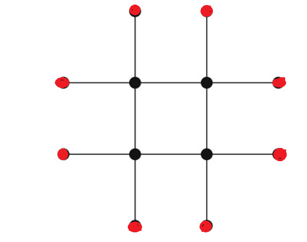
   Figure 5. The corona graph ${\operatorname{\mathsf{C}}_{4}}\circ{(2\operatorname{\mathsf{K}}_{1})}$ (see Definition 5.8).

   Definition 5.9.

   [38] The edge corona of $\mathsf{G}_{1}$ and $\mathsf{G}_{2}$, denoted by ${\mathsf{G}_{1}}\diamondsuit\hskip 0.85355pt{\mathsf{G}_{2}}$, is defined as the graph obtained by taking one copy of $\mathsf{G}_{1}$ and $m_{1}=\bigl{|}\operatorname{\mathsf{E}}(\mathsf{G}_{1})\bigr{|}$ copies of $\mathsf{G}_{2}$, and then connecting, for each $j\in[m_{1}]$, the two end-vertices of the $j$-th edge of $\mathsf{G}_{1}$ to every vertex in the $j$-th copy of $\mathsf{G}_{2}$ (see Figure 6).

   

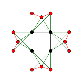
   Figure 6. The edge-corona graph ${\operatorname{\mathsf{C}}_{4}}\diamondsuit\hskip 0.85355pt{\operatorname{\mathsf{P}}_{3}}$ (see Definition 5.9.

   Definition 5.10.

   Let $\mathsf{G}_{1}$ and $\mathsf{G}_{2}$ be graphs with disjoint vertex sets of $n_{1}$ and $n_{2}$ vertices, respectively. Let $Du(\mathsf{G}_{1})$ be the duplication graph of $\mathsf{G}_{1}$ with vertex set $\operatorname{\mathsf{V}}(\mathsf{G}_{1})\cup\mathrm{U}(\mathsf{G}_{1})$, where $\operatorname{\mathsf{V}}(\mathsf{G}_{1})=\{v_{1},\ldots,v_{n_{1}}\}$ and with the duplicated vertex set $\mathrm{U}(\mathsf{G}_{1})=\{u_{1},\ldots,u_{n_{1}}\}$ (see Definition 5.7). The duplication corona graph, denoted by ${\mathsf{G}_{1}}\boxminus{\mathsf{G}_{2}}$, is the graph obtained from $\mathrm{Du}(\mathsf{G}_{1})$ and $n_{1}$ copies of $\mathsf{G}_{2}$ by connecting, for each $i\in[n_{1}]$, the vertex $v_{i}\in\operatorname{\mathsf{V}}(\mathsf{G}_{1})$ of the graph $\mathrm{Du}(\mathsf{G}_{1})$ to every vertex in the $i$-th copy of $\mathsf{G}_{2}$ (see Figure 7).

   

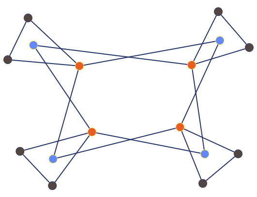
   Figure 7. The duplication corona graph ${\operatorname{\mathsf{C}}_{4}}\boxminus{\operatorname{\mathsf{K}}_{2}}$ (see Definition 5.10).

   Definition 5.11.

   Let $\mathsf{G}_{1}$ and $\mathsf{G}_{2}$ be graphs with disjoint vertex sets of $n_{1}$ and $n_{2}$ vertices, respectively. Let $\mathrm{Du}(\mathsf{G}_{1})$ be the duplication graph of $\mathsf{G}_{1}$ with the vertex set $\mathrm{V}(\mathsf{G}_{1})\cup\mathrm{U}(\mathsf{G}_{1})$, where $\mathrm{V}(\mathsf{G}_{1})=\{v_{1},\ldots,v_{n_{1}}\}$ and the duplicated vertex set $\mathrm{U}(\mathsf{G}_{1})=\{u_{1},\ldots,u_{n_{1}}\}$ (see Definition 5.7). The duplication neighborhood corona, denoted by $\mathsf{G}_{1}\boxbar\mathsf{G}_{2}$, is the graph obtained from $\mathrm{Du}(\mathsf{G}_{1})$ and $n_{1}$ copies of $\mathsf{G}_{2}$ by connecting the neighbors of the vertex $v_{i}\in\operatorname{\mathsf{V}}(\mathsf{G}_{1})$ of $\mathrm{Du}(\mathsf{G}_{1})$ to every vertex in the $i$-th copy of $\mathsf{G}_{2}$ for $i\in[n_{1}]$ (see Figure 8).

   

   Figure 8. The duplication neighborhood corona $\operatorname{\mathsf{K}}_{3}\boxbar\operatorname{\mathsf{K}}_{2}$ (see Definition 5.11).

   Definition 5.12.

   Let $\mathsf{G}_{1}$ and $\mathsf{G}_{2}$ be graphs with disjoint vertex sets of $n_{1}$ and $n_{2}$ vertices, respectively. Let $\mathrm{Du}(\mathsf{G}_{1})$ be the duplication graph of $\mathsf{G}_{1}$ with vertex set $\operatorname{\mathsf{V}}(\mathsf{G_{1}})\cup\mathrm{U}(\mathsf{G}_{1})$, where $\operatorname{\mathsf{V}}(\mathsf{G}_{1})=\{v_{1},\ldots,v_{n_{1}}\}$ is the vertex set of $\mathsf{G}_{1}$ and $\mathrm{U}(\mathsf{G}_{1})=\{u_{1},\ldots,u_{n_{1}}\}$ is the duplicated vertex set. The duplication edge corona, denoted by ${\mathsf{G}_{1}}\boxplus{\mathsf{G}_{2}}$, is the graph obtained from $\mathrm{Du}(\mathsf{G}_{1})$ and $\bigl{|}\operatorname{\mathsf{E}}(\mathsf{G}_{1})\bigr{|}$ copies of $\mathsf{G}_{2}$ by connecting each of the two vertices $v_{i},v_{j}\in\operatorname{\mathsf{V}}(\mathsf{G}_{1})$ of $\mathrm{Du}(\mathsf{G}_{1})$ to every vertex in the $k$-th copy of $\mathsf{G}_{2}$ whenever $\{v_{i},v_{j}\}=e_{k}\in\operatorname{\mathsf{E}}(\mathsf{G}_{1})$ (see Figure 9).

   

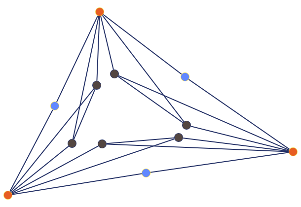
   Figure 9. The duplication edge corona ${\operatorname{\mathsf{K}}_{3}}\boxplus{\operatorname{\mathsf{K}}_{2}}$ (see Definition 5.12).

   Definition 5.13.

   Consider two graphs $\mathsf{G}_{1}$ and $\mathsf{G}_{2}$ with $n_{1}$ and $n_{2}$ vertices and, respectively. The closed neighborhood corona of $\mathsf{G}_{1}$ and $\mathsf{G}_{2}$, denoted by ${\mathsf{G}_{1}}\,\underline{\boxtimes}\,{\mathsf{G}_{2}}$, is a new graph obtained by creating $n_{1}$ copies of $\mathsf{G}_{2}$. Each vertex of the $i^{th}$ copy of $\mathsf{G}_{2}$ is then connected to the $i^{th}$ vertex and neighborhood of the $i^{th}$ vertex of $\mathsf{G}_{1}$ (see Figure 10).

   

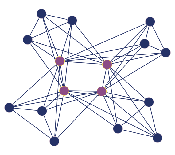
   Figure 10. The closed neighborhood corona of the 4-length cycle $\operatorname{\mathsf{C}}_{4}$ and the triangle $\operatorname{\mathsf{K}}_{3}$, denoted by ${\operatorname{\mathsf{C}}_{4}}\,\underline{\boxtimes}\,{\operatorname{\mathsf{K}}_{3}}$ (see Definition 5.13).

   Theorem 5.14.

   [3] Let $\mathsf{G}_{1},\mathsf{H}_{1}$ be $r_{1}$-regular, cospectral graphs, and let $\mathsf{G}_{2}$ and $H_{2}$ be $r_{2}$-regular, cospectral, and nonisomorphic (NICS) graphs. Then, the following holds:

   • The duplication corona graphs ${\mathsf{G}_{1}}\boxminus{\mathsf{G}_{2}}$ and ${\mathsf{H}_{1}}\boxminus{\mathsf{H}_{2}}$ are $\{\operatorname{\mathbf{A}},\operatorname{\mathbf{L}},\operatorname{\mathbf{Q}}\}$-NICS irregular graphs.

   • The duplication neighborhood corona $\mathsf{G}_{1}\boxbar\mathsf{G}_{2}$ and $\mathsf{H}_{1}\boxbar H_{2}$ are $\{\operatorname{\mathbf{A}},\operatorname{\mathbf{L}},\operatorname{\mathbf{Q}}\}$-NICS irregular graphs.

   • The duplication edge corona ${\mathsf{G}_{1}}\boxplus{\mathsf{G}_{2}}$ and ${\mathsf{H}_{1}}\boxplus{\mathsf{H}_{2}}$ are $\{\operatorname{\mathbf{A}},\operatorname{\mathbf{L}},\operatorname{\mathbf{Q}}\}$-NICS irregular graphs.

   Question 5.15.

   Are the irregular graphs in Theorem 5.14 also cospectral with respect to the normalized Laplacian matrix?

   Theorem 5.16.

   [60] Let $\mathsf{G}_{1}$ and $\mathsf{G}_{2}$ be cospectral regular graphs, and let $\mathsf{H}$ be an arbitrary graph. Then, the following holds:

   • The closed neighborhood corona ${\mathsf{G}_{1}}\,\underline{\boxtimes}\,{\mathsf{H}}$ and ${\mathsf{G}_{2}}\,\underline{\boxtimes}\,{\mathsf{H}}$ are $\{\operatorname{\mathbf{A}},\operatorname{\mathbf{L}},\operatorname{\mathbf{Q}}\}$-NICS irregular graphs.

   • The closed neighborhood corona ${\mathsf{H}}\,\underline{\boxtimes}\,{\mathsf{G}_{1}}$ and ${\mathsf{H}}\,\underline{\boxtimes}\,{\mathsf{G}_{2}}$ are $\{\operatorname{\mathbf{A}},\operatorname{\mathbf{L}},\operatorname{\mathbf{Q}}\}$-NICS irregular graphs.

   Question 5.17.

   Are the irregular graphs in Theorem 5.16 also cospectral with respect to the normalized Laplacian matrix?

   5.5. Graphs constructions based on the subdivision and bipartite incidence graphs

   Definition 5.18.

   [21] Let $\mathsf{G}$ be a graph. The subdivision graph of $\mathsf{G}$, denoted by $\mathrm{S}(\mathsf{G})$, is obtained from $\mathsf{G}$ by inserting a new vertex into every edge of $\mathsf{G}$. Subdivision is the process of adding a new vertex along an edge, effectively splitting the edge into two edges connected in series through the new vertex (see Figure 11).

   

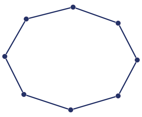
   Figure 11. The subdivision graph of a $4$-length cycle, denoted by $\mathrm{S}(\operatorname{\mathsf{C}}_{4})$, which is an $8$-length cycle $\operatorname{\mathsf{C}}_{8}$ (see Definition 5.18).

   Definition 5.19.

   [53] Let $\mathsf{G}$ be a graph. The bipartite incidence graph of $\mathsf{G}$, denoted by $\mathrm{B}(\mathsf{G})$, is a bipartite graph constructed as follows: For each edge $e\in\mathsf{G}$, a new vertex $u_{e}$ is added to the vertex set of $\mathsf{G}$. The vertex $u_{e}$ is then made adjacent to both endpoints of $e$ in $\mathsf{G}$ (see Figure 12).

   

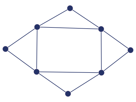
   Figure 12. The bipartite incidence graph of a length-4 cycle $\operatorname{\mathsf{C}}_{4}$, denoted by $\mathrm{B}(\operatorname{\mathsf{C}}_{4})$ (see Definition 5.19).

   Let $\mathsf{G}_{1}$ and $\mathsf{G}_{2}$ be two vertex-disjoint graphs with $n_{1}$ and $n_{2}$ vertices, and $m_{1}$ and $m_{2}$ edges, respectively. Four binary operations on these graphs are defined as follows.

   Definition 5.20.

   The subdivision-vertex-bipartite-vertex join of graphs $\mathsf{G}_{1}$ and $\mathsf{G}_{2}$, denoted $\mathrm{S}(\mathsf{G}_{1})\,\ddot{\vee}\,\mathrm{B}(\mathsf{G}_{2})$, is the graph obtained from $\mathrm{S}(\mathsf{G}_{1})$ and $\mathrm{B}(\mathsf{G}_{2})$ by connecting each vertex of $\operatorname{\mathsf{V}}(\mathsf{G}_{1})$ (that is the subset of the original vertices in the vertex set of $\mathrm{S}(\mathsf{G}_{1})$) with every vertex of $\operatorname{\mathsf{V}}(\mathsf{G}_{2})$ (that is the subset of the original vertices in the vertex set of $\mathrm{B}(\mathsf{G}_{2})$).

   By Definitions 5.18, 5.19, and 5.20, it follows that the graph $\mathrm{S}(\mathsf{G}_{1})\,\ddot{\vee}\,\mathrm{B}(\mathsf{G}_{2})$ has $n_{1}+n_{2}+m_{1}+m_{2}$ vertices and $n_{1}n_{2}+2m_{1}+3m_{2}$ edges. Figure 13 displays the graph $\mathrm{S}(\operatorname{\mathsf{C}}_{4})\,\ddot{\vee}\,\mathrm{B}(\operatorname{\mathsf{P}}_{3})$.

   

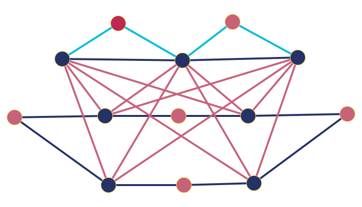
   Figure 13. The graph $\mathrm{S}(\operatorname{\mathsf{C}}_{4})\,\ddot{\vee}\,\mathrm{B}(\operatorname{\mathsf{P}}_{3})$ (see Definition 5.20). The black vertices represent the vertices of the length-4 cycle $\operatorname{\mathsf{C}}_{4}$ and the vertices of the path $\operatorname{\mathsf{P}}_{3}$. The additional vertices in the subdivision graph $\mathrm{S}(\operatorname{\mathsf{C}}_{4})$ are the four red vertices located at the bottom of this figure (as shown in Figure 11). Similarly, the additional vertices in the bipartite incidence graph of the path $\operatorname{\mathsf{P}}_{3}$ are the two red vertices located at the top of this figure. The edges of the graph include the following: edges connecting each black vertex of $\operatorname{\mathsf{C}}_{4}$ to each black vertex of $\operatorname{\mathsf{P}}_{3}$, edges between the black and red vertices at the bottom of the figure (that correspond to the subdivision of $\operatorname{\mathsf{C}}_{4}$), and the four (light blue) edges connecting the two top red vertices to the top black vertices of the figure (that correspond to the bipartite incidence graph of $\operatorname{\mathsf{P}}_{3}$).

   Definition 5.21.

   The subdivision-edge-bipartite-edge join of $\mathsf{G}_{1}$ and $\mathsf{G}_{2}$, denoted by $\mathrm{S}(\mathsf{G}_{1})\,\overset{\raisebox{-2.84544pt}{$=$}}{\vee}\,\mathrm{B}(\mathsf{G}_{2})$, is the graph obtained from $\mathrm{S}(\mathsf{G}_{1})$ and $\mathrm{B}(\mathsf{G}_{2})$ by connecting each vertex of $\operatorname{\mathsf{V}}(\mathrm{S}(\mathsf{G}_{1}))\setminus\operatorname{\mathsf{V}}(\mathsf{G}_{1})$ (that is the subset of the added vertices in the vertex set of $\mathrm{S}(\mathsf{G}_{1})$) with every vertex of $\operatorname{\mathsf{V}}(\mathrm{B}(\mathsf{G}_{2}))\setminus\operatorname{\mathsf{V}}(\mathsf{G}_{2})$ (that is the subset of the added vertices in the vertex set of $\mathrm{B}(\mathsf{G}_{2})$).

   By Definitions 5.18, 5.19, and 5.21, it follows that the graph $\mathrm{S}(\mathsf{G}_{1})\,\overset{\raisebox{-2.84544pt}{$=$}}{\vee}\,\mathrm{B}(\mathsf{G}_{2})$ has $n_{1}+n_{2}+m_{1}+m_{2}$ vertices and $m_{1}m_{2}+2m_{1}+3m_{2}$ edges. Figure 14 displays the graph $\mathrm{S}(\operatorname{\mathsf{C}}_{4})\,\overset{\raisebox{-2.84544pt}{$=$}}{\vee}\,\mathrm{B}(\operatorname{\mathsf{P}}_{3})$.

   

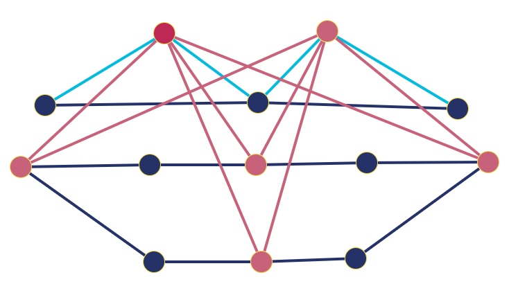
   Figure 14. The graph $\mathrm{S}(\operatorname{\mathsf{C}}_{4})\,\overset{\raisebox{-2.84544pt}{$=$}}{\vee}\,\mathrm{B}(\operatorname{\mathsf{P}}_{3})$ (see Definition 5.21). In comparison to Figure 13, edges connecting each black vertex of $\operatorname{\mathsf{C}}_{4}$ to each black vertex of $\operatorname{\mathsf{P}}_{3}$ are deleted and replaced in this figure by edges connecting each red vertex of $\operatorname{\mathsf{C}}_{4}$ to each red vertex of $\operatorname{\mathsf{P}}_{3}$.

   Definition 5.22.

   The subdivision-edge-bipartite-vertex join of $\mathsf{G}_{1}$ and $\mathsf{G}_{2}$, denoted by $\mathrm{S}(\mathsf{G}_{1})\,{\overset{\raisebox{-7.11317pt}{$\stackrel{{\scriptstyle\rule{7.11317pt}{0.14226pt}}}{{\cdot}}$}}{\vee}}\hskip 2.84544pt\mathrm{B}(\mathsf{G}_{2})$, is the graph obtained from $\mathrm{S}(\mathsf{G}_{1})$ and $\mathrm{B}(\mathsf{G}_{2})$ by connecting each vertex of $\operatorname{\mathsf{V}}(\mathrm{S}(\mathsf{G}_{1}))\setminus\operatorname{\mathsf{V}}(\mathsf{G}_{1})$ (that is the subset of the added vertices in the vertex set of $\mathrm{S}(\mathsf{G}_{1})$) with every vertex of $\operatorname{\mathsf{V}}(\mathsf{G}_{2})$ (that is the subset of the original vertices in the vertex set of $\mathrm{B}(\mathsf{G}_{2})$).

   By Definitions 5.18, 5.19, and 5.22, it follows that the graph $\mathrm{S}(\mathsf{G}_{1})\,{\overset{\raisebox{-7.11317pt}{$\stackrel{{\scriptstyle\rule{7.11317pt}{0.14226pt}}}{{\cdot}}$}}{\vee}}\hskip 2.84544pt\mathrm{B}(\mathsf{G}_{2})$ has $n_{1}+n_{2}+m_{1}+m_{2}$ vertices and $m_{1}n_{2}+2m_{1}+3m_{2}$ edges. Figure 15 displays the graph $\mathrm{S}(\operatorname{\mathsf{C}}_{4})\,{\overset{\raisebox{-7.11317pt}{$\stackrel{{\scriptstyle\rule{7.11317pt}{0.14226pt}}}{{\cdot}}$}}{\vee}}\hskip 2.84544pt\mathrm{B}(\operatorname{\mathsf{P}}_{3})$.

   

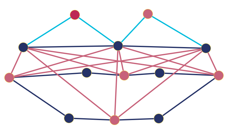
   Figure 15. The graph $\mathrm{S}(\operatorname{\mathsf{C}}_{4})\,{\overset{\raisebox{-7.11317pt}{$\stackrel{{\scriptstyle\rule{7.11317pt}{0.14226pt}}}{{\cdot}}$}}{\vee}}\hskip 2.84544pt\mathrm{B}(\operatorname{\mathsf{P}}_{3})$ (see Definition 5.22). In comparison to Figure 13, edges connecting each black vertex of $\operatorname{\mathsf{C}}_{4}$ to each black vertex of $\operatorname{\mathsf{P}}_{3}$ are deleted and replaced in this figure by edges connecting each red vertex of $\operatorname{\mathsf{C}}_{4}$ to each black vertex of $\operatorname{\mathsf{P}}_{3}$.

   Definition 5.23.

   The subdivision-vertex-bipartite-edge join of $\mathsf{G}_{1}$ and $\mathsf{G}_{2}$, denoted by $\mathrm{S}(\mathsf{G}_{1})\,{\overset{\raisebox{0.0pt}{$\stackrel{{\scriptstyle\cdot}}{{\rule{7.11317pt}{0.14226pt}}}$}}{\vee}}\hskip 2.84544pt\mathrm{B}(\mathsf{G}_{2})$, is the graph obtained from $\mathrm{S}(\mathsf{G}_{1})$ and $\mathrm{B}(\mathsf{G}_{2})$ by connecting each vertex of $\operatorname{\mathsf{V}}(\mathsf{G}_{1})$ (that is the subset of the original vertices in the vertex set of $\mathrm{S}(\mathsf{G}_{1})$) with every vertex of $\operatorname{\mathsf{V}}(\mathrm{B}(\mathsf{G}_{2}))\setminus\operatorname{\mathsf{V}}(\mathsf{G}_{2})$ (that is the subset of the added vertices in the vertex set of $\mathrm{B}(\mathsf{G}_{2})$).

   By Definitions 5.18, 5.19, and 5.23, it follows that the graph $\mathrm{S}(\mathsf{G}_{1})\,{\overset{\raisebox{0.0pt}{$\stackrel{{\scriptstyle\cdot}}{{\rule{7.11317pt}{0.14226pt}}}$}}{\vee}}\hskip 2.84544pt\mathrm{B}(\mathsf{G}_{2})$ has $n_{1}+n_{2}+m_{1}+m_{2}$ vertices and $n_{1}m_{2}+2m_{1}+3m_{2}$ edges. Figure 16 displays the graph $\mathrm{S}(\operatorname{\mathsf{C}}_{4})\,{\overset{\raisebox{0.0pt}{$\stackrel{{\scriptstyle\cdot}}{{\rule{7.11317pt}{0.14226pt}}}$}}{\vee}}\hskip 2.84544pt\mathrm{B}(\operatorname{\mathsf{P}}_{3})$.

   

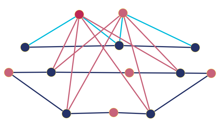
   Figure 16. The graph $\mathrm{S}(\operatorname{\mathsf{C}}_{4})\,{\overset{\raisebox{0.0pt}{$\stackrel{{\scriptstyle\cdot}}{{\rule{7.11317pt}{0.14226pt}}}$}}{\vee}}\hskip 2.84544pt\mathrm{B}(\operatorname{\mathsf{P}}_{3})$ (see Definition 5.23). In comparison to Figure 13, edges connecting each black vertex of $\operatorname{\mathsf{C}}_{4}$ to each black vertex of $\operatorname{\mathsf{P}}_{3}$ are deleted and replaced in this figure by edges connecting each black vertex of $\operatorname{\mathsf{C}}_{4}$ to each red vertex of $\operatorname{\mathsf{P}}_{3}$.

   We next present the main result of this subsection, which motivates the four binary graph operations introduced in Definitions 5.20–5.23.

   Theorem 5.24.

   [26] Let $\mathsf{G}_{i}$ , $\mathsf{H}_{i}$, where $i\in\{1,2\}$, be regular graphs, where $\mathsf{G}_{1}$ need not be different from $\mathsf{H}_{1}$. If $\mathsf{G}_{1}$ and $\mathsf{H}_{1}$ are $\operatorname{\mathbf{A}}$-cospectral, and $\mathsf{G}_{2}$ and $\mathsf{H}_{2}$ are $\operatorname{\mathbf{A}}$-cospectral, then

   • $\mathrm{S}(\mathsf{G}_{1})\,\ddot{\vee}\,\mathrm{B}(\mathsf{G}_{2})$ and $\mathrm{S}(\mathsf{H}_{1})\,\ddot{\vee}\,\mathrm{B}(\mathsf{H}_{2})$ are irregular $\{\operatorname{\mathbf{A}},\operatorname{\mathbf{L}},{\bf{\mathcal{L}}}\}$-NICS graphs.

   • $\mathrm{S}(\mathsf{G}_{1})\,\overset{\raisebox{-2.84544pt}{$=$}}{\vee}\,\mathrm{B}(\mathsf{G}_{2})$ and $\mathrm{S}(\mathsf{H}_{1})\,\overset{\raisebox{-2.84544pt}{$=$}}{\vee}\,\mathrm{B}(\mathsf{H}_{2})$ are irregular $\{\operatorname{\mathbf{A}},\operatorname{\mathbf{L}},{\bf{\mathcal{L}}}\}$-NICS graphs.

   • $\mathrm{S}(\mathsf{G}_{1})\,{\overset{\raisebox{-7.11317pt}{$\stackrel{{\scriptstyle\rule{7.11317pt}{0.14226pt}}}{{\cdot}}$}}{\vee}}\hskip 2.84544pt\mathrm{B}(\mathsf{G}_{2})$ and $\mathrm{S}(\mathsf{H}_{1})\,{\overset{\raisebox{-7.11317pt}{$\stackrel{{\scriptstyle\rule{7.11317pt}{0.14226pt}}}{{\cdot}}$}}{\vee}}\hskip 2.84544pt\mathrm{B}(\mathsf{H}_{2})$ are irregular $\{\operatorname{\mathbf{A}},\operatorname{\mathbf{L}},{\bf{\mathcal{L}}}\}$-NICS graphs.

   • $\mathrm{S}(\mathsf{G}_{1})\,{\overset{\raisebox{0.0pt}{$\stackrel{{\scriptstyle\cdot}}{{\rule{7.11317pt}{0.14226pt}}}$}}{\vee}}\hskip 2.84544pt\mathrm{B}(\mathsf{G}_{2})$ and $\mathrm{S}(\mathsf{H}_{1})\,{\overset{\raisebox{0.0pt}{$\stackrel{{\scriptstyle\cdot}}{{\rule{7.11317pt}{0.14226pt}}}$}}{\vee}}\hskip 2.84544pt\mathrm{B}(\mathsf{H}_{2})$ are irregular $\{\operatorname{\mathbf{A}},\operatorname{\mathbf{L}},{\bf{\mathcal{L}}}\}$-NICS graphs.

   In light of Theorem 5.24, the following questions naturally arises.

   Question 5.25.

   Are the graphs in Theorem 5.24 also cospectral with respect to the signless Laplacian matrix (i.e., $\operatorname{\mathbf{Q}}$-cospectral)?

   5.6. Connected irregular NICS graphs

   The examination of cospectrality in regular graphs with respect to the adjacency, Laplacian, signless Laplacian, and normalized Laplacian matrices is simpler than for irregular graphs. This is because it suffices to verify cospectrality for only one of these matrices. Specifically, two regular graphs are $X$-cospectral for some $X\in\{\operatorname{\mathbf{A}},\operatorname{\mathbf{L}},\operatorname{\mathbf{Q}},{\bf{\mathcal{L}}}\}$ if and only if they are cospectral with respect to all these matrices (see Corollary 3.8). This naturally raises the following question, which was posed by Butler [12]:

   Question 5.26.

   [12] Are there pairs of irregular graphs that are $\{\operatorname{\mathbf{A}},\operatorname{\mathbf{L}},\operatorname{\mathbf{Q}},{\bf{\mathcal{L}}}\}$-NICS, i.e., $X$-NICS with respect to every $X\in\{\operatorname{\mathbf{A}},\operatorname{\mathbf{L}},\operatorname{\mathbf{Q}},{\bf{\mathcal{L}}}\}$?

   This question remained open until two coauthors of this paper recently proposed a method for constructing pairs of irregular graphs that are $X$ cospectral with respect to every $X\in\{\operatorname{\mathbf{A}},\operatorname{\mathbf{L}},\operatorname{\mathbf{Q}},{\bf{\mathcal{L}}}\}$, providing explicit constructions [37]. Building on that work, another coauthor of this paper demonstrated in [56] that for every even integer $n\geq 14$, there exist two connected, irregular $\{\operatorname{\mathbf{A}},\operatorname{\mathbf{L}},\operatorname{\mathbf{Q}},{\bf{\mathcal{L}}}\}$-NICS graphs on $n$ vertices with identical independence, clique, and chromatic numbers, yet distinct Lovász $\vartheta$-functions. We now present the preliminary definitions required to outline the relevant results in [37] and [56], and the construction of such cospectral irregular $X$-NICS graphs for all $X\in\{\operatorname{\mathbf{A}},\operatorname{\mathbf{L}},\operatorname{\mathbf{Q}},{\bf{\mathcal{L}}}\}$.

   Definition 5.27 (Neighbors splitting join of graphs).

   [47] Let $\mathsf{G}$ and $\mathsf{H}$ be graphs with disjoint vertex sets, and let $\operatorname{\mathsf{V}}(\mathsf{G})=\{v_{1},\ldots,v_{n}\}$. The neighbors splitting (NS) join of $\mathsf{G}$ and $\mathsf{H}$ is obtained by adding vertices $v^{\prime}_{1},\ldots,v^{\prime}_{n}$ to the vertex set of $\mathsf{G}\vee\mathsf{H}$ and connecting $v^{\prime}_{i}$ to $v_{j}$ if and only if $\{v_{i},v_{j}\}\in\operatorname{\mathsf{E}}(\mathsf{G})$. The NS join of $\mathsf{G}$ and $\mathsf{H}$ is denoted by $\mathsf{G}\,\underline{\vee}\,\mathsf{H}$.

   Definition 5.28 (Nonneighbors splitting join of graphs [36, 37]).

   Let $\mathsf{G}$ and $\mathsf{H}$ be graphs with disjoint vertex sets, and let $\operatorname{\mathsf{V}}(\mathsf{G})=\{v_{1},\ldots,v_{n}\}$. The nonneighbors splitting (NNS) join of $\mathsf{G}$ and $\mathsf{H}$ is obtained by adding vertices $v^{\prime}_{1},\ldots,v^{\prime}_{n}$ to the vertex set of $\mathsf{G}\vee\mathsf{H}$ and connecting $v^{\prime}_{i}$ to $v_{j}$, with $i\neq j$, if and only if $\{v_{i},v_{j}\}\not\in\operatorname{\mathsf{E}}(\mathsf{G})$. The NNS join of $\mathsf{G}$ and $\mathsf{H}$ is denoted by $\mathsf{G}\,\uuline{\vee}\,\mathsf{H}$.

   Remark 5.29.

   In general, $\mathsf{G}\,\underline{\vee}\,\mathsf{H}\not\cong\mathsf{H}\,\underline{\vee}\,\mathsf{G}$ and $\mathsf{G}\,\uuline{\vee}\,\mathsf{H}\not\cong\mathsf{H}\,\uuline{\vee}\,\mathsf{G}$ (unless $\mathsf{G}\cong\mathsf{H}$).

   Example 5.30 (NS and NNS join of graphs [37]).

   Figure 17 shows the NS and NNS joins of the path graphs $\operatorname{\mathsf{P}}_{4}$ and $\operatorname{\mathsf{P}}_{2}$, denoted by $\operatorname{\mathsf{P}}_{4}\,\underline{\vee}\,\operatorname{\mathsf{P}}_{2}$ and $\operatorname{\mathsf{P}}_{4}\,\uuline{\vee}\,\operatorname{\mathsf{P}}_{2}$, respectively.

   

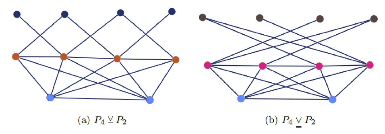
   Figure 17. The neighbors splitting (NS) and nonneighbors splitting (NNS) joins of the path graphs $\operatorname{\mathsf{P}}_{4}$ and $\operatorname{\mathsf{P}}_{2}$ are depicted, respectively, on the left and right-hand sides of this figure. The NS and NNS joins of graphs are, respectively, denoted by $\operatorname{\mathsf{P}}_{4}\,\underline{\vee}\,\operatorname{\mathsf{P}}_{2}$ and $\operatorname{\mathsf{P}}_{4}\,\uuline{\vee}\,\operatorname{\mathsf{P}}_{2}$ [37].

   Theorem 5.31 (Irregular $\{\operatorname{\mathbf{A}},\operatorname{\mathbf{L}},\operatorname{\mathbf{Q}},\bf{\mathcal{L}}\}$-NICS graphs).

   Let $\mathsf{G}_{1}$ and $\mathsf{H}_{1}$ be regular and cospectral graphs, and let $\mathsf{G}_{2}$ and $\mathsf{H}_{2}$ be regular, nonisomorphic, and cospectral (NICS) graphs. Then, the following statements hold:

   1. The NS-join graphs $\mathsf{G}_{1}\,\underline{\vee}\,\mathsf{G}_{2}$ and $\mathsf{H}_{1}\,\underline{\vee}\,\mathsf{H}_{2}$ are irregular $\{\operatorname{\mathbf{A}},\operatorname{\mathbf{L}},\operatorname{\mathbf{Q}},\bf{\mathcal{L}}\}$-NICS graphs.

   2. The NNS join graphs $\mathsf{G}_{1}\,\uuline{\vee}\,\mathsf{G}_{2}$ and $\mathsf{H}_{1}\,\uuline{\vee}\,\mathsf{H}_{2}$ are irregular $\{\operatorname{\mathbf{A}},\operatorname{\mathbf{L}},\operatorname{\mathbf{Q}},\bf{\mathcal{L}}\}$-NICS graphs.

   The proof of Theorem 5.31 is provided in [36, 37], and it relies heavily on the notion of the Schur complement and Schur lemma (see Theorem 2.2). The interested reader is referred to the recently published paper [37] for further details.

   Relying on Theorem 5.31, the following result is stated and proved in [56].

   Theorem 5.32 (On irregular NICS graphs).

   For every even integer $n\geq 14$, there exist two connected, irregular $\{\operatorname{\mathbf{A}},\operatorname{\mathbf{L}},\operatorname{\mathbf{Q}},\bf{\mathcal{L}}\}$-NICS graphs on $n$ vertices with identical independence, clique, and chromatic numbers, yet their Lovász $\vartheta$-functions are distinct.

   That result is in fact strengthened in Section 4.2 of [56], and the interested reader is referred to that paper for further details. The proof of Theorem 5.32 is also constructive, providing explicit such graphs.

   6. Open questions and outlook

   We conclude this paper by highlighting some of the most significant open questions in the fascinating area of research related to cospectral nonisomorphic graphs and graphs determined by their spectrum, leaving them as topics for further future study.

   6.1. Haemers’ conjecture

   Haemers’ conjecture [34, 35], a prominent topic in spectral graph theory, posits that almost all graphs are uniquely determined by their adjacency spectrum. This conjecture suggests that for large graphs, the probability of having two non-isomorphic graphs, on a large number of vertices, sharing the same adjacency spectrum is negligible. The conjecture has inspired extensive research, including studies on specific graph families, cospectrality, and algebraic graph invariants, contributing to deeper insights into the relationship between graph structure and eigenvalues. Haemers’ conjecture is stated formally as follows.

   Definition 6.1.

   For $n\in\mathbb{N}$, let $I(n)$ to be the numbers of distinct graphs on $n$ vertices, up to isomorphism. For $\mathcal{X}\subseteq\{\operatorname{\mathbf{A}},\operatorname{\mathbf{L}},\operatorname{\mathbf{Q}},{\bf{\mathcal{L}}},\overline{\operatorname{\mathbf{A}}},\overline{\operatorname{\mathbf{L}}},\overline{\operatorname{\mathbf{Q}}},\overline{{\bf{\mathcal{L}}}}\}$, let $\alpha_{\mathcal{X}}(n)$ be the number of $\mathcal{X}$-DS graphs on $n$ vertices, up to isomorphism, and (for the sake of simplicity of notation) let $\alpha(n)\triangleq\alpha_{\{A\}}(n)$

   Conjecture 6.2.

   [34] For sufficiently large $n$, almost all of the graphs are DS, i.e.,

   (6.1) $$\lim_{n\rightarrow\infty}\frac{\alpha(n)}{I(n)}=1.$$

   Several results lend support to this conjecture [34, 42, 63], but a complete proof in its full generality remains elusive. By [33], the number of graphs with $n$ vertices up to isomorphism is

   (6.2) $$I(n)=\bigl{(}1-\epsilon(n)\bigr{)}\,\frac{2^{n(n-1)/2}}{n!},$$

   where $\underset{n\rightarrow\infty}{\lim}\epsilon(n)=0$. By Stirling’s approximation for $n!$ and straightforward algebra, $I(n)$ can be verified to be given by

   (6.3) $$I(n)=2^{\frac{n(n-1)}{2}\;\bigl{(}1-\epsilon(n)\bigr{)}}.$$

   It is shown in [42] that the number of DS graphs on $n$ vertices is at least $e^{cn}$ for some constant $c>0$ (see also our earlier discussion in Section 4.4). In light of Remark 3.6, it is natural to generalize Conjecture 6.2 to the following:

   Question 6.3.

   For what minimal subset $\mathcal{X}\subset\{\operatorname{\mathbf{A}},\operatorname{\mathbf{L}},\operatorname{\mathbf{Q}},{\bf{\mathcal{L}}},\overline{\operatorname{\mathbf{A}}},\overline{\operatorname{\mathbf{L}}},\overline{\operatorname{\mathbf{Q}}},\overline{{\bf{\mathcal{L}}}}\}$ (if any) does the limit

   (6.4) $$\lim_{n\rightarrow\infty}\frac{\alpha_{\mathcal{X}}(n)}{I(n)}=1$$

   hold?

   Some computer results somewhat support Haemers’ Conjecture. Approximately $80\%$ of the graphs with $12$ vertices are DS [9]. A new class of graphs is defined in [63], offering an algorithmic method for finding all the $\{\operatorname{\mathbf{A}},\overline{\operatorname{\mathbf{A}}}\}$-cospectral mates of a graph $\mathsf{G}$ in this class (i.e., graphs that are $\{\operatorname{\mathbf{A}},\overline{\operatorname{\mathbf{A}}}\}$-cospectral with $\mathsf{G}$). Using this algorithm, they found that out of $10,000$ graphs with $50$ vertices, chosen uniformly at random from this class, at least $99.5\%$ of them were $\{\operatorname{\mathbf{A}},\overline{\operatorname{\mathbf{A}}}\}$-DS.

   6.2. DS properties of structured graphs

   This paper explores various structures of graph families determined by their spectrum with respect to one or more of their associated matrices, as well as the related problem of constructing pairs of nonisomorphic graphs that are cospectral with respect to some or all of these matrices. Several questions are interspersed throughout the paper (see Questions 5.15, 5.17, 5.25, and 5.26), which remain open for further study.

   In addition to serving as a survey to introduce readers to this fascinating area of spectral graph determination, this paper also derives the adjacency spectrum of the family of Turán graphs. It also suggests a new alternative proof to Theorem 3.3 in [48], asserting that this important family of structured graphs is determined by its adjacency spectrum (see Theorems 4.20 and 4.23). Since these graphs are generally bi-regular multipartite graphs (i.e., their vertices have only two possible degrees, which in this case are consecutive integers), this therefore does not necessarily imply that they are determined by the spectrum of other associated matrices, such as the Laplacian, signless Laplacian, or normalized Laplacian matrices. Determining whether this holds is currently an open question.

   Another newly obtained proof presented in this paper refers to a necessary and sufficient condition in [48] for complete bipartite graphs to be $\operatorname{\mathbf{A}}$-DS (see Theorem 4.9 and Remark 4.10 here). These graphs are also bi-regular, and the two possible vertex degrees can differ by more than one. Both of these newly obtained proofs, discussed in Section 4, provide insights into the broader question of which (structured) multipartite graphs are determined by their adjacency spectrum or, more generally, by the spectra of some of their associated matrices.

   Even if Haemers’ conjecture is eventually proved in its full generality, it remains surprising when a new family of structured graphs is shown to be DS (or $X$-DS, more generally). This is because for certain structured graphs, such as strongly regular graphs and trees, their spectra often fail to uniquely determine them [23, 24]. This stark contrast between the fact that almost all random graphs of high order are likely to be DS and the existence of interesting structured graphs that are not DS has significant theoretical and practical implications.

   In addition to the questions posed earlier in this paper, we raise the following additional concrete question:

   • By Theorem 4.36, the family of generalized friendship graphs $F_{p,q}$ is ${\bf{\mathcal{L}}}$-DS. What can be determined about whether these graphs are also DS with respect to other associated matrices (e.g., $\operatorname{\mathbf{A}}$, $\operatorname{\mathbf{L}}$, $\operatorname{\mathbf{Q}}$ or matrices that marge some of these matrices [49])?

   We speculate that the DS property of a graph correlates, to some extent, with the number of symmetries the graph possesses. While this statement should be taken with a grain of salt, we hypothesize that the size of the automorphism group of a graph can partially indicate whether it is DS.

   A justification for this claim is that the automorphism group of a graph reflects its symmetries, which can influence the eigenvalues of its adjacency matrix. Highly symmetric graphs (i.e., those with large automorphism groups) often exhibit eigenvalue multiplicities and patterns that are shared by other nonisomorphic graphs, making such graphs less likely to be DS. Conversely, graphs with trivial automorphism groups are typically less symmetric and may have eigenvalues that uniquely determine their structure, increasing the likelihood that they are DS. As noted in [33], almost all graphs have trivial automorphism groups. This observation aligns with the conjecture that most graphs are DS, as the absence of symmetry reduces the likelihood of two nonisomorphic graphs sharing the same spectrum.

   However, it should be noted that the DS property of graphs is not solely determined by their automorphism groups. Specifically, a graph with a large automorphism group can still be DS if its eigenvalues uniquely encode its structure. For instance, certain strongly regular graphs with high symmetry are known to be DS (e.g., the length-5 cycle graph $\operatorname{\mathsf{C}}_{5}$, and the Petersen graph are DS, among some other strongly regular graphs that are known to be DS). Conversely, graphs with trivial automorphism groups are not guaranteed to be DS; in such cases, the spectrum might not capture enough structural information to uniquely determine the graph. Typically, graphs with few distinct eigenvalues seem to be the hardest graphs to distinguish by their spectrum. As noted in [25], it seems that most graphs with few eigenvalues (e.g., strongly regular graphs) are not determined by their spectrum, which served as one of the motivations of the work in [25] in studying graphs whose normalized Laplacian has three eigenvalues.

   To conclude, the size of the automorphism group of a graph can provide some indication of whether it is DS, but it is not a definitive criterion. While large automorphism groups often correlate with the graph not being DS due to shared eigenvalues among nonisomorphic graphs, this is not an absolute rule. The DS property depends on a complex interplay between a graph’s symmetry, structure, and spectral properties. Therefore, the claim should be understood as a general observation that requires careful qualification to account for exceptions.

References

- 1 A. Abiad, W. Haemers, Cospectral graphs and regular orthogonal matrices of level 2. Electron. J. Combin. vol 19, no. 3, paper P13, 2012. https://doi.org/10.37236/2383
- 2 A. Abiad, B. Brimkov, J. Breen, T.R. Cameron, H. Gupta, R. Villagran, “Constructions of cospectral graphs with different zero forcing numbers,” Electron. J. Linear Algebra, vol. 38, pp. 280–294, May 2022. https://doi.org/10.13001/ela.2022.6737
- 3 C. Adiga, B. R. Rakshith, K. N. Subba Krishna. Spectra of some new graph operations and some new class of integral graphs. Iranian Journal of Mathematical Sciences and Informatics, vol. 13, no. 1, pp. 51–65, May 2018. Available from http://ijmsi.ir/article-1-755-en.html
- 4 M. Aigner, G. M. Ziegler, Proofs from the book, Sixth Edition, Springer, Berlin, Germany, 2018. Available from: https://link.springer.com/book/10.1007/978-3-662-57265-8
- 5 S. Bang, E. R. van Dam, J. H. Koolen, Spectral characterization of the Hamming graphs. Linear Algebra and its Applications 429(11-12): 2678-–2686, December 2008. https://doi.org/10.1016/j.laa.2007.10.026
- 6 A. Berman, D. M. Chen, Z. B. Chen, W. Z. Liang, X. D. Zhang. A family of graphs that are determined by their normalized Laplacian spectra. Linear Algebra and its Applications, vol. 548, pp. 66–76, 2018. https://doi.org/10.1016/j.laa.2018.03.001
- 7 R. Boulet. Disjoint unions of complete graphs characterized by their Laplacian spectrum. Electronic Journal of Linear Algebra, vol. 18, no. 1, pp. 773–783, January 2009. https://doi.org/10.13001/1081-3810.1344
- 8 A. E. Brouwer and W. H. Haemers. Spectra of Graphs. Springer Science & Business Media, 2011. https://doi.org/10.1007/978-1-4614-1939-6.
- 9 A. E. Brouwer, E. Spence. Cospectral graphs on 12 vertices. Electronic Journal of Combinatorics, vol. 16, no. 1, paper 20, pp. 1–3, June 2009. https://doi.org/10.37236/258
- 10 C. Bu and J. Zhou. Signless Laplacian spectral characterization of the cones over some regular graphs. Linear Algebra and its Applications, vol. 436, no. 9, pp. 3634–3641, 2012. https://doi.org/10.1016/j.laa.2011.12.035
- 11 S. Butler. Eigenvalues and Structures of Graphs. University of California, San Diego, 2008. Available from https://escholarship.org/uc/item/3qd9g26t
- 12 S. Butler. A note about cospectral graphs for the adjacency and normalized Laplacian matrices. Linear and Multilinear Algebra, 2010, 58(3), 387–390. Taylor & Francis. https://doi.org/10.1080/03081080902722741
- 13 S. Butler and J. Grout, “A construction of cospectral graphs for the normalized Laplacian,” Electronic Journal of Combinatorics, vol. 18, no. 1, paper P231, pp. 1–20, December 2011. https://doi.org/10.37236/718
- 14 S. Butler. A gentle introduction to the normalized Laplacian, IMAGE 53, pp 19-27, Fall 2014. Online available from https://www.stevebutler.org/research/publications
- 15 S. Butler. Algebraic aspects of the normalized Laplacian. Recent Trends in Combinatorics, pp. 295–315, Springer, 2016. doi:https://doi.org/10.1007/978-3-319-24298-9_13
- 16 S. Butler and K. Heysse, A cospectral family of graphs for the normalized Laplacian found by toggling. Linear Algebra and its Applications, vol. 507, pp. 499–512, October 2016. https://doi.org/10.1016/j.laa.2016.06.033
- 17 A. Cayley. A theorem on trees.Quart. J. Pure Appl. Math. 23: 376–378. (1889)
- 18 F. R. K. Chung, Spectral Graph Theory, American Mathematical Society, 1997. https://doi.org/10.1090/cbms/092
- 19 S. M. Cioabǎ, W. H. Haemers, J. R. Vermette, W. Wong. The graphs with all but two eigenvalues equal to . Journal of Algebraic Combinatorics, 41(3), 887-897 (2015). https://doi.org/10.1007/s10801-014-0557-y
- 20 D. M. Cvetković, M/ Doob, and H. Sacs. Spectra of Graphs: Theory and Applications, Johann Ambrosius Barth Verlag, third edition, 1995.
- 21 D. M. Cvetković, P. Rowlinson, and S. Simić, An Introduction to the Theory of Graph Spectra. Cambridge University Press, 2009. https://doi.org/10.1017/CBO9780511801518
- 22 D. M. Cvetković, P. Rowlinson, and S. Simić, “Signless Laplacians of finite graphs,” Linear Algebra and Applications, vol. 423, pp. 155–171, 2007. https://doi.org/10.1016/j.laa.2007.01.009
- 23 E. R. van Dam and W. H. Haemers, “Which graphs are determined by their spectrum?,” Linear Algebra and Applications, 343 (2003), 241–272. https://doi.org/10.1016/S0024-3795(03)00483-X
- 24 E. R. van Dam and W. H. Haemers, “Developments on spectral characterizations of graphs,” Discrete Mathematics, vol. 309, no. 3, pp. 576–589, February 2009. http://dx.doi.org/10.1016/j.disc.2008.08.019
- 25 E. R. van Dam and G. R. Omidi, “Graphs whose normalized Laplacian has three eigenvalues,” Linear Algebra and its Applications, vol. 435, no. 10, pp. 2560–2569, November 2011. https://doi.org/10.1016/j.laa.2011.02.005
- 26 A. Das and P. Panigrahi. Construction of simultaneous cospectral graphs for adjacency, Laplacian and normalized Laplacian matrices. Kragujevac Journal of Mathematics, 47(6):947-964 (2023) http://dx.doi.org/10.46793/KgJMat2306.947D
- 27 S. Dutta, B. Adhikari, Construction of cospectral graphs, J. Algebraic Combin., 52 (2020), 215–235. https://doi.org/10.1007/s10801-019-00900-y
- 28 P. Erdös. On a problem in graph theory. The Mathematical Gazette , Volume 47 , Issue 361 , October 1963 , pp. 220 - 223. https://doi.org/10.2307/3613396
- 29 F. Esser and F. Harary. On the spectrum of a complete multipartite graph. European Journal of Combinatorics, 1(3):211–218, 1980. https://doi.org/10.1016/S0195-6698(80)80004-7
- 30 R. Frucht and F. Harary, On the corona of two graphs. (1970)
- 31 H.H. Günthard and H. Primas, Zusammenhang von Graphentheorie und MO-Theorie von Molekeln mit Systemen konjugierter Bindungen, Helv. Chim. Acta, vol. 39, no. 6, pp. 1645–1653, 1956.
- 32 C. Godsil and B. McKay, Constructing cospectral graphs, Aequationes Mathematicae, vol. 25, pp. 257–268, December 1982. https://doi.org/10.1007/BF02189621
- 33 C. Godsil and G. Royle, Algebraic Graph Theory, Graduate Texts in Mathematics, vol. 27, Springer, New York, 2001. https://doi.org/10.1007/978-1-4613-0163-9
- 34 W. Haemers, Are almost all graphs determined by their spectrum?, Not. S. Afr. Math. Soc. 47.1 (2016): 42-45. Available at https://www.researchgate.net/publication/304747396
- 35 W. Haemers. Proving spectral uniqueness of graphs. In Combinatorics 2024, Carovigno, Italy, June 2024. Plenary Talk.
- 36 S. Hamud, Contributions to Spectral Graph Theory, Ph.D. dissertation, Technion-Israel Institute of Technology, Haifa, Israel, 2023.
- 37 S. Hamud, A. Berman, New constructions of nonregular cospectral graphs, Special Matrices, 12 (2024), 1–21. https://doi.org/10.1515/spma-2023-0109.
- 38 Y. Hou and W. C. Shiu, The spectrum of the edge corona of two graphs. The Electronic Journal of Linear Algebra, vol. 20, pp. 586–594, September 2010. https://doi.org/10.13001/1081-3810.1395
- 39 M. R. Kannan, S. Pragada, H. Wankhede, “On the construction of cospectral nonisomorphic bipartite graphs,” Discrete Mathematics, vol. 345, no. 8, pp. 1–8, August 2022. https://doi.org/10.1016/j.disc.2022.112916.
- 40 G. Kirchhoff, On the Solution of the Equations Obtained from the Investigation of the Linear Distribution of Galvanic Currents, IRE Transactions on Circuit Theory, vol. 5, no. 1, pp. 4-7 (1958) https://doi.org/10.1109/TCT.1958.1086426.
- 41 N. Kogan, A. Berman. Characterization of completely positive graphs. Discrete Mathematics, 114(1-3), 297-304 (1993). https://doi.org/10.1016/0012-365X(93)90374-3
- 42 I. Koval, M. Kwan. Exponentially many graphs are determined by their spectrum. The Quarterly Journal of Mathematics, vol. 75, no. 3, pp. 869–899, September 2024. https://doi.org/10.1093/qmath/haae030
- 43 N. Krupnik and A. Berman, “The graphs of pyramids are determined by their spectrum,” Linear Algebra and its Applications, 2024. https://doi.org/10.1016/j.laa.2024.04.029
- 44 Y. Lin, J. Shu, and Y. Meng, “Laplacian spectrum characterization of extensions of vertices of wheel graphs and multi-fan graphs,” Computers & Mathematics with Applications, vol. 60, no. 7, pp. 2003–2008, 2010. https://doi.org/10.1016/j.camwa.2010.07.035
- 45 X. Liu, Y. Zhang, and X. Gui. The multi-fan graphs are determined by their Laplacian spectra. Discrete Mathematics, vol. 308, no. 18, pp. 4267–4271, September 2008. https://doi.org/10.1016/j.disc.2007.08.002
- 46 L. Lovász, “On the Shannon capacity of a graph,” IEEE Transactions on Information Theory, vol. 25, no. 1, pp. 1–7, January 1979. https://doi.org/10.1109/TIT.1979.1055985
- 47 Z. Lu, X. Ma, and M. Zhang, “Spectra of graph operations based on splitting graph,” Journal of Applied Analysis and Computation, vol. 13, no. 1, pp. 133–155, February 2023. https://doi.org/10.11948/20210446
- 48 H. Ma and H. Ren, “On the spectral characterization of the union of complete multipartite graph and some isolated vertices,” Discrete Mathematics, vol. 310, pp. 3648–3652, September 2010. https://doi.org/10.1016/j.disc.2010.09.004
- 49 V. Nikiforov, “Merging the - and -spectral theories,” Applicable Analysis and Discrete Mathematics, vol. 11, no. 1, pp. 81–107, 2017. https://doi.org/10.2298/AADM1701081N
- 50 C. S. Oliveira, L. S. de Lima, N. M. M. de Abreu, and S. Kirkland, “Bounds on the -spread of a graph,” Linear Algebra and its Applications, vol. 432, no. 9, pp. 2342–2351, April 2010. https://doi.org/10.1016/j.laa.2009.06.011
- 51 G. R. Omidi and K. Tajbakhsh. Starlike trees are determined by their Laplacian spectrum. Linear Algebra and its Applications, 422(2-3):654-658, 2007. https://doi.org/10.1016/j.laa.2006.11.028.
- 52 B. N. Parlett, The symmetric eigenvalue problem. Classics in Applied Mathematics, 1998.
- 53 T. Pisanski and B. Servatius, Configurations from a Graphical Viewpoint, Springer, 2013. https://doi.org/10.1007/978-0-8176-8364-1
- 54 E. Sampathkumar and H. B. Walikar, On the splitting graph of a graph. Karnatak Univ. Sci (13): 13–16. (1980) Available from https://www.researchgate.net/publication/269007309
- 55 I. Sason, Observations on Lovász -function, graph capacity, eigenvalues, and strong products, Entropy, 25 (2023), 104, 1–40. https://doi.org/10.3390/e25010104.
- 56 I. Sason. Observations on graph invariants with the Lovász -function. AIMS Mathematics (2024) 9(6): 15385-15468. https://doi.org/10.3934/math.2024747
- 57 J. Schur, Über Potenzreihen, die im Innern des Einheitskreises beschränkt sind. (1917): 205-232.
- 58 A. J. Schwenk, Almost all trees are cospectral, F. Harary (Ed.), New Directions in the Theory of Graphs, Academic Press, New York pp. 275–307. (1973)
- 59 J. H Smith. Some properties of the spectrum of a graph. Combinatorial Structures and their applications, p. 403–406, 1970.
- 60 B. Sonar, R. Srivastava. On the spectrum of closed neighborhood corona product of graph and its application. July 2024. http://dx.doi.org/10.48550/arXiv.2407.05653.
- 61 P. Turán. On an external problem in graph theory. Mat. Fiz. Lapok, 48:436–452, 1941.
- 62 J. Wang, F. Belardo, Q. Huang, and B. Borovićanin. On the two largest -eigenvalues of graphs. Discrete Mathematics, 310(21):2858-2866, 2010. https://doi.org/10.1016/j.disc.2010.06.030.
- 63 W. Wang, W. Wang. Haemers’ conjecture: an algorithmic perspective. Experimental Mathematics, 1-28. (2024). https://doi.org/10.1080/10586458.2024.2337229
- 64 J. Ye, M. Liu, and Z. Stanić, Two classes of graphs determined by their signless Laplacian spectrum. Linear Algebra and Its Applications, vol. 708, pp. 159–172, March 2025. https://doi.org/10.1016/j.laa.2024.10.029.
-
•