Learning physical unknowns from hydrodynamic shock and material interface features in ICF capsule implosions

Abstract

In high energy density physics (HEDP) and inertial confinement fusion (ICF), predictive modeling is complicated by uncertainty in parameters that characterize various aspects of the modeled system, such as those characterizing material properties, equation of state (EOS), opacities, and initial conditions. Typically, however, these parameters are not directly observable. What is observed instead is a time sequence of radiographic projections using X-rays. In this work, we define a set of sparse hydrodynamic features derived from the outgoing shock profile and outer material edge, which can be obtained from radiographic measurements, to directly infer such parameters. Our machine learning (ML)-based methodology involves a pipeline of two architectures, a radiograph-to-features network (R2FNet) and a features-to-parameters network (F2PNet), that are trained independently and later combined to approximate a posterior distribution for the parameters from radiographs. We show that the estimated parameters can be used in a hydrodynamics code to obtain density fields and hydrodynamic shock and outer edge features that are consistent with the data. Finally, we demonstrate that features resulting from an unknown EOS model can be successfully mapped onto parameters of a chosen analytical EOS model, implying that network predictions are learning physics, with a degree of invariance to the underlying choice of EOS model.

1 Introduction

1.1 Inferring physical parameters from radiographic data

Simulation plays a major role in the experimental design and analysis of radiation hydrodynamic behavior in high energy density physics (HEDP) and inertial confinement fusion (ICF), e.g. [1, 2, 3, 4, 5, 6], as well as in the discovery of material properties of objects made to undergo strong deformations in material science and shock physics [7, 8, 9]. Improving the predictive skill of these simulations is likely to be key in ensuring continued progress in the design of robust burning ICF capsules [10, 11]. However, in many of these applications predictive modeling is complicated by the inherent uncertainty in parameters used to model material properties, equation of state (EOS), opacities, and constitutive relationships, as well as complex physics associated with the initial conditions, e.g., the laser drive in ICF experiments [12, 13, 14, 15, 16, 17]. Furthermore, understanding uncertainties in the initial conditions as well as the role of measurement uncertainty are both crucial in improving the predictive behavior of simulations. Consequently, dynamic experimentation plays a crucial role in calibrating models to improve simulations of hydrodynamic behavior and the discovery of material properties.

Historically to investigate material properties such as EOS and constitutive relationships, e.g., material strength in shock physics and material science, an impulse-response approach is used wherein the velocity trace response of the material specimen to an impulse is measured using velocity interferometry [18, 19, 20]. Indeed, the development of laser interferometry enabled the time-resolved measurement of the velocity from a reflecting surface [18]. This allowed for the measurement of the free surface and window interface velocities in dynamic compression experiments [21]. These measurements have yielded valuable data on compressive behavior and strength of materials during both shock compression and release [21, 22, 23, 24, 25]. Characterization of Rayleigh-Taylor (RT) and Richtmyer-Meshkov (RM) instabilities, e.g., in terms of perturbation growth rates, are also widely used to examine constitutive relationships in shock physics, and to quantify material strength in materials undergoing extreme deformation [26, 27, 28, 29, 30, 31, 32, 33, 34, 35, 36, 37]. Furthermore, these investigations enable examinations of asymmetry in geometric perturbations due to, e.g., manufacturing, as well as velocity perturbations, i.e drive asymmetries, to both understand and design control strategies to minimize the resulting hydrodynamic instabilities that degrade ICF performance [17, 38, 39, 40, 41, 42].

Figure 1: Example plots of the density evolution (a) and the various RMI profiles representing each inner surface perturbation profile at a fixed time frame $n=40$ (b). The images are 150x150 pixels representing the domain $\left[0,\frac{15}{44}L\right]\times\left[0,\frac{15}{44}L\right]$.

To examine RT and RM instabilities in extreme temperature and pressure conditions in a laboratory setting, spherical convergent geometries are necessary. These extreme conditions play a fundamental role in the design of robust burning ICF capsules. Figure 1 presents a time-history of an evolving instability in which an outward going shock interacts with a perturbed surface which gives rise to a RM instability. In this setting radiographic measurements serve as the primary means to identify key features such as peaks and troughs and to quantify empirical growth rates, which then serve as reference data to validate theoretical and computational models. Indeed, experimental facilities now provide ultrafast proton [43], neutron [44], and x-ray [45] imaging capabilities, typically in the form of radiographic projections to characterize RMI behavior [46, 47, 48, 49, 37, 50, 51, 48]. While experimental RMI growth rates have been previously obtained in both planar and cylindrical geometries [52, 53, 54, 55, 56, 57, 58], validation of growth rates in spherical convergent geometries in which a reflected shock impacts a perturbed surface has not yet been achieved. This is in part due to the impact of noise/scatter in the radiographic images. The presence of scatter and noise observed in a typical radiograph, as demonstrated in Figure 2, does not enable an accurate determination of the peak and troughs.

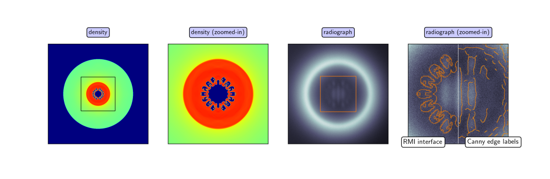
Figure 2: Sample $(r,z)$ projection of the density (1^st column), zoomed-in view of the Richtmyer-Meshkov interface (2^nd column), synthetic radiograph (3^rd columns), and a zoomed-in view of the radiograph (4^th columns) labeled with the RMI interface (left half) and Canny edge labels (right half).

Consequently, characterization of the initial conditions responsible for the instability as well as material properties characterizing the growth rates demands new techniques to solve this inverse problem. One such approach to resolve this difficulty has recently been proposed,[59] which utilizes the robust features of the outgoing shock to characterize the growth rates of the instability via a density reconstruction of the radiographic images. The success of this methodology is founded in the fact that the outgoing shock encodes sufficient information to enable machine learning techniques to learn a mapping between a sequence of outgoing shocks and the corresponding density fields. In this work we propose to utilize the outgoing shock as well as outer material edge as robust features to enable parameter estimation and estimation of the initial conditions.

1.2 A machine learning (ML)-based inverse mapping based on shock and outer edge features

Here we develop a framework to construct machine-learning-based inverse mappings directly from experimental radiographic images to the underlying physical parameters and initial perturbations in ICF settings systems. We assume a governing physical model given by the compressible Euler equations, dropping higher-order effects of radiation for ease of testing and development, analogous to recent work [60], and we assume unknown initial conditions and material properties for the governing Euler equations. As such, we build upon previous work that demonstrates the ability to both learn a sequence of density fields as well as parameters from a sequence of radiographic features to diagnose asymmetries in the drive of ICF capsules, by utilizing an inert gas as a surrogate for the D-T fuel to enable extraction of the outgoing shock [61, 47, 62]. We note that recent work at the National Ignition Facility has been performed using a silicon dopant  [63]. Furthermore, by subsequent design optimization to minimize asymmetries, improved neutron yields can be realized. Our specific problem description is one in which an ICF-like shell is imploded with an initially perturbed surface as depicted in Figure˜3. Upon collapse, the generation of a shock forms on axis and subsequently rebounds, interacting with the perturbed surface of the shell and initiates a RM instability. We posit that the outer material edge, outgoing shock, and their evolution encode sufficient information from the instability to identify the underlying simplified Mie-Grüneisenn EOS parameters and structure of the initial shell perturbation and velocity. Moreover, the shock and edge profiles are some of the few robust and identifiable features in dynamic radiographic images of HEDP experiments, which in general are subject to noise and scattering effects, and correspond to a projected areal mass rather than a primary hydrodynamic variable such as density. Thus broadly, we aim to calibrate material models and initial conditions to be consistent with the outgoing shock and edge profile, a problem of data-assimilation [64]. There are many approaches to data assimilation, and here we review some of the prominent techniques, before concluding with our specific machine-learning-based approach.

Variational data-assimilation minimizes a cost function comparing a forward model/simulation with experimental data [64]. Although the field of data assimilation often uses emulators or surrogate models for forward evolution, when considering the full “high-order” forward model, variational data assimilation is a subclass of the broader mathematical fields of optimal control (unknown parameters/models) and inverse problems (unknown initial state) based on variational principles [65]. When the governing equations are dynamic partial differential equations (PDEs), each of these are PDE-constrained optimization problems. Indeed for problems related to ICF, we believe it is critical to incorporate a high-order representation of the physics in a forward model, rather than working exclusively with some form of surrogate. As mentioned previously, shock interface and evolution provide some of the most robust and predictive information available, and surrogate or machine learning models that can accurately capture and track nonlinearly evolving and interacting shocks, let alone the formation of instabilities, remains a largely open question, e.g., see [66].

PDE-constrained optimization is indeed a rigorous approach to inverse and optimal control problems, but is also very challenging computationally in terms of cost and memory [67]. Each gradient descent iteration requires a full forward and adjoint solution of the underlying PDE, in addition to storing a full physical solution to linearize about at every time point simulated, in order to compute a gradient in the adjoint pass; additional difficulties arise in maintaining geometric structure [68]. This has led to significant recent interest in machine-learning based approaches to solving inverse and optimal control problems in computational physics. Perhaps the most popular are so-called physics informed neural networks (PINNs) [69], where the differentials of the underlying PDE are evaluated directly within a neural network via automatic differentiation. Then in training the PINN model, the forward and adjoint pass of classical gradient descent can be evaluated relatively cheaply purely based on automatic differentiation capabilities inherent to NNs. PINNs and many variations thereof have shown significant success in computational physics, particularly for optimal control and inverse problems, where the computational cost and required coding infrastructure are significantly less than a traditional adjoint-based optimization [70].

However, there is an additional major hurdle to overcome in calibrating models based on experimental radiographic data obtained from dynamic imaging experiments. That is, these experiments typically do not provide direct data on primary physical variables. Instead, the observations are images formed via both the primary signal as well as the scattered radiation signal along with the noise of the radiographic system and characteristics of the detection system. Indeed, extraction of the primary state variable, i.e. density, of the time-series of 2d noisy radiographic projections continues to be a challenge [47, 59, 71]. Consequently, the computation of gradients based on radiographs, or extracted features and material interfaces as used here, necessary for PDE-constrained optimization or PINNs-like ML models immediately precludes the direct application of these methods.

Consequently, in this work we develop machine learning architectures that directly take in a low-dimensional time-series of radiographic images, extract the outgoing shock and outer material edge profiles, and estimate the corresponding EOS parameters as well as initial shell conditions. The generation of data is discussed in Section˜2 and the machine learning (ML)-based parameter estimation pipeline is introduced in Section˜2.4. Using numerical simulations, we then demonstrate in Section˜3 that our ML architecture is able to successfully recover EOS material parameters, initial shell profiles, and velocity to reproduce the observed shock and edge features, demonstrating that the time series of shock profiles does indeed encode sufficient information to infer these parameters with high accuracy. Moreover, in numerical simulation of HEDP, EOS is typically represented via underlying model assumptions or tabulated data models. We demonstrate that an expansive parameter model is sufficient to represent unknown models, in the sense that we can use an ML architecture trained on an underlying EOS model, $M_{1}$, and output parameters of $M_{1}$ for a time-series of shock profiles generated with a different underlying EOS model, $M_{2}$, that lead to a consistent time-series of shock profiles as those originally generated based on $M_{2}$. In this sense, our ML model is learning structure from the underlying physics, above a specific choice of EOS parameterization needed for numerical simulation.

2 Methods

2.1 Generation of density time series

As a representative problem of a double shell ICF capsule implosion, we study shock propagation in a time-dependent pseudo-3D density profile, created by the implosion of a perturbed spherical metallic shell into a medium of gas. We utilize air in lieu of D-T in order to enable examination of the out-going shock which would otherwise be obscured by the burning plasma once the hot spot is formed. We rely on the effects of a non-spherical perturbation and variation in initial velocity to provide distinct behavior in the late-time shock evolution. We assume azimuthal symmetry, therefore the density at any time can be described in 2D cylindrical coordinates $(r,z)$, but the solution remains 3-dimensional via the symmetry assumption. Additionally, we focus on the Mie-Grüneisen (MG) EOS model. We then generate a large set of data for variations in the inner shell perturbation, initial shell velocity, and EOS parameters, where each data sample contains a time series of the resulting hydrodynamic density field. Simulations are performed on a $440\times 440$ uniform Cartesian grid on a computational domain given by the quarter-plane $[0,L]\times[0,L]$, where $L=341$ $\mu$m. The uniform grid cell size is $\Delta r=\Delta z=\frac{L}{440}$. The metallic shell is made of Tantalum and its density is initially uniform at a value of 16.65 g/cc.

The shell perturbations are specified by adding harmonic perturbations to the inner surface of a spherical Tantalum shell, which can be described as the set of coordinates $(r_{\rm in}(u),z_{\rm in}(u))$ satisfying $r_{\rm in}(u)^{2}+z_{\rm in}(u)^{2}=\left(R_{\rm in}+\sum_{k=1}^{8}F_{k}\cos(2ku)\right)^{2}$, where $u\in[0,\pi/2]$, ${R_{\rm in}=248}$ $\mu$m, $F_{k}$, $k=1,\dots,8$, are coefficients of the perturbation corresponding to the $k^{\rm th}$ cosine harmonic. The outer surface of the shell is a sphere with radius ${R_{\rm out}=310}$ $\mu$m. There are 20 different inner surface perturbation profiles considered in our dataset. The corresponding coefficients are recorded in Table 4. Figure 3 presents an initial perturbation given to the interior shell. As an initial condition, the shell is given a uniform implosion velocity, $v_{\rm impl}$, in the direction of the origin to initiate an implosion. We include 4 choices of implosion velocity in our dataset.

Figure 3: (a): Example double shell capsule specification based on the 1.06 MJ yield design from Ref. [72]. (b): 3D mock-up of a shell with a perturbation on the interior surface. (c): projection of the shell onto $(r,z)$ coordinates. The inner radius is parameterized by the angle, $u$ between the white dotted line and the $r$ axis. (d): Plot of the 20 separate profiles for radius of the perturbed inner surface verses angle $u$.

The MG EOS [73] can be parameterized in analytical form as

$$p\left(\chi,T\right)=\frac{\rho_{0}c_{s}^{2}\chi\left(1-\frac{1}{2}\Gamma_{0}\chi\right)}{(1-s_{1}\chi)^{2}}+\Gamma_{0}\rho_{0}c_{V}(T-T_{0}),$$ (1)

where $\chi=1-\frac{\rho_{0}}{\rho}$, $\rho_{0}$ and $T_{0}$ are the reference density and temperature, respectively, $c_{s}$ is the speed of sound, $\Gamma_{0}$ is the Grüneisen parameter at the reference state, $s_{1}$ is the slope of the linear shock Hugoniot curve, and $c_{V}$ is the specific heat capacity at constant volume. Out of these parameters, we keep the reference density $\rho_{0}$ fixed at 16.65 g/cc and the reference temperature $T_{0}$ fixed at 0.0253 eV, leaving EOS parameters $\{c_{s},\,s_{1},\,\Gamma_{0},\,c_{V}\}$ as unknown. Table 1 presents the EOS parameter values we sample in generating our training data set.

Options	1	2	3	4	5
$\Gamma_{0}$	1.6	1.7	1.76	1.568	1.472
$s_{1}$	1.22	1.464	1.342
$c_{s}$ [m/s]	339000	372900	305100	355000
$c_{V}$ $[{\rm erg}\;{\rm g}^{-1}\;{\rm eV}^{-1}]$	$1.6\times 10^{10}$	$1.76\times 10^{10}$	$1.44\times 10^{10}$

Table 1: Matrix of parameter values used to develop the simulated dataset. All combinations of above parameters are used to simulate our data.

Altogether, the dataset realizes every unique parameter combination in a 6-dimensional parameter cube with $14,400$ total simulations. Each hydrodynamic simulation is comprised of density field snapshots at later times when the instability is present. We label these times as $n=0,1,\dots,40$. An example of a density time series is shown in Figure 1a. Once the shock propagating through the gas converges to the axis, a reflected shock from the axis then propagates outward and interacts with the perturbed inner Tantalum edge, creating a RMI. The topology of this interior evolves as depicted in Figure 1b. The expanding shock proceeds to propagate into the non-constant dynamic density background. We chose frames corresponding to the time instants at $n=25,30,35,40$ to train the network in our studies.

2.2 Generation of Synthetic Radiographs

Synthetic radiographs are produced at each time step using the imaging model described in [47]. This model involves first obtaining the areal mass for the gas and metal using the cone beam projection provided by the ASTRA Toolbox [74]. The final transmission includes contamination from several noise terms, which contains correlated blur, scatter, and a Poisson noise field. Figure 2 shows an example of a density field at time index 40 and a synthetic radiograph.

2.3 Identification of shock and edge features

One of the primary aspects of the dynamics is the evolution of the inner air-metal interface, i.e., the growth of the instability. This is because the passage of the incoming and outgoing shocks through this interface renders it unstable to the RMI. Considering temporally evolving simulations, we are interested in times when the instability on this interface has permitted the growth of perturbations to the extent that the inner air-metal interface displays significant asymmetry. As such, we assume that the interface as identified by a feature extraction procedure is not robust due to sensitivities with respect to the chosen imaging plane. This is in contrast to the shock and outer edge features that we assume are robust. Nevertheless, because of the shock’s passage across the unstable inner air-metal interface, we expect the stably evolving shock to be imprinted with a set of perturbations that can be reliably identified in a noisy radiograph [47].

Shock and edge features are extracted at each time for each sequence of density fields. Our feature extraction algorithm consists of two stages: (i) using the maximal gradient to detect computational cells where the features are present; and (ii) subpixel feature extraction. For subpixel feature detection, we use the partial-area algorithm [75], generalized to quadratic density functions assumed on both sides of the feature. Specifically, we examine the neighborhood of every pixel where the feature is present, assuming that the density on both sides of the discontinuity may be described by a function which is quadratic in both variables. Following the original algorithm [75], we then fit for the shape of the feature with the constraint that the mass along the stripes in the neighborhood of the feature matches the integrated density. The result is a parametric representation of the shock and edge as a function of polar angle [59]. We compressed these shock and outer edge features into a low-dimensional representation in terms of cosine harmonic coefficients, $r^{(i)}(\theta)=\sum_{j=0}^{N^{(i)}}F^{(i)}_{j}\cos(2j\theta),$ for $i={\rm shock},{\rm edge}$. We found that $N^{(\rm shock)}=8$ and $N^{(\rm edge)}=5$ can represent the shock and edge features with sufficient accuracy across the dataset.

2.4 Parameter estimation machine learning pipeline

Our ML-based parameter estimation pipeline is composed of two architectures, a radiograph-to-features network (R2FNet) and a features-to-parameters (F2PNet) network, described respectively in Sections B and C. R2FNet and F2PNet are trained separately and later combined for testing. F2PNet also consists of a forward model, which is a surrogate for the parameters-to-features mapping. In Section 3, we evaluate the model’s ability to recover parameters from radiographs through examining self consistency with respect to features produced by both the surrogate and true forward model. We consider a time sequence of $n\in\{25,30,35,40\}$, which corresponds to times where the outgoing shock is fully formed in the metal and the RMI has entered a linear growth phase. The dataset consisting of triplets of radiographs, features, and parameters is randomly partitioned into training, validation, and testing sets corresponding to 80%, 10%, and 10% of the data, respectively.

3 Results

3.1 Model Performance on Testing Set

Figure 4: Prediction performance of the parameter estimation pipeline on the testing set. (a): Scatter plots depicting the agreement between the scaled features predicted using R2FNet on the test set of noisy radiographs (vertical axis) and the corresponding scaled ground truth features (horizontal) axis in the testing set. (b): Line plots depicting the agreement between the scaled parameters predicted using F2PNet on the features predicted from R2FNet (violin plots representing the data range and distribution) and scaled ground truth parameters (diagonal lines) in the testing set. The correlation coefficients are shown in their respective plots.

After training R2PNet and F2PNet, parameter estimations were performed on each data point in the testing set. R2PNet is used to predict shock and edge features for each radiograph. These predicted features are then inputted into the decoder of F2PNet for 25 different realizations of the generator to produce a distribution of parameter estimates. The feature and parameter predictions are illustrated in Figure 4. The horizontal axes correspond to ground truth values and the vertical axes correspond to the predictions. In the case of the parameter predictions, violin plots are shown on the vertical axis corresponding to the distribution of network predictions. Correlation coefficients are shown in each of the plots.

As seen by the plots, R2FNet is able to predict the edge and the lower order harmonics of the shock (e.g. $F_{0}$ through $F_{4}$) with high correlation, while correlation is degraded for higher order harmonics of the shock (e.g. $F_{1}$ through $F_{8}$). Despite this, F2PNet is able to predict all parameters except for $\Gamma_{0}$ and $c_{v}$ with high correlation. This demonstrates that $\Gamma_{0}$ and $c_{v}$ are likely insensitive parameters for late-time shock and edge features and the rest of the parameters can be predicted with reasonable accuracy. The violin plots show that the range of estimates can be highly variable, however the distributions seem to be closely centered around the diagonal line denoting ground truth. Note that $F_{0},F_{5},$ and $F_{7}$ are omitted since there is no variance in these parameters in the dataset.

We now evaluate the capability of the trained forward model along with the self-consistency of the network. Feature predictions are obtained by inputting the parameter estimates from the decoder on the testing set into the forward model. Figure 5 shows histograms of the $L_{2}$ and $L_{\infty}$ errors for the shock and edge curves resulting from the feature predictions. The majority of the reconstructions are accurate to within one pixel of error. Figure 5 shows example feature reconstructions corresponding to the best, median, and worst $L_{2}$ errors for both the shock and edge.

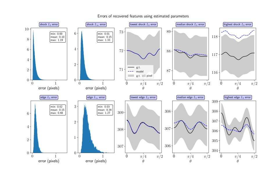
Figure 5: Errors of reconstructed shock and edge features reconstructed using the forward model on parameters estimates from the decoder on the testing set. The top row corresponds to shock features and the bottom row corresponds to edge features. The first two columns show histograms of the $L_{2}$ and $L_{\infty}$ errors, respectively, and the last three columns show examples of reconstructed shock and edge features (dotted blue line) representing the extreme cases of the distributions superimposed over the ground truth feature (black line) and an error bar of $\pm$1 pixels (gray region).

3.2 Model Sensitivity Studies

We now consider the effect of the training set size on predictive capability. Models are trained with various training set sizes ranging from 10% to 70%. After training, correlation coefficients are computed for each parameter and shown in Table 2. Monotonic improvement is generally observed across all parameters with $c_{v}$ as an exception. It is clear that there is significant degradation in performance when the sample size is too small. Additionally, we observe that the degradation is dependent on the parameter. We remark that, relative to other parameters, $F_{2},F_{4}$, and $F_{8},$ are learned with reasonable skill with the smallest training set; for harmonics, this makes sense given that $F_{2},F_{4}$, and $F_{8}$ are more densely sampled compared to other parameters (see Figure 4). Note that even at 30% of the available training data, the correlation coefficients for many of the parameters do not drop significantly. These insights are important for our future work on 3D problems that are not assumed to be symmetric, since the data generation is significantly more computationally expensive.

Training Set Size Performance Study

$f_{N_{d}}$	$F_{1}$	$F_{2}$	$F_{3}$	$F_{4}$	$F_{6}$	$F_{8}$	$v_{\rm impl}$	$\Gamma_{0}$	$s_{1}$	$c_{s}$	$c_{v}$
10%	0.575	0.954	0.607	0.900	0.595	0.880	0.536	0.007	0.604	0.631	-0.009
30%	0.866	0.976	0.893	0.956	0.903	0.972	0.914	0.011	0.942	0.899	-0.016
50%	0.924	0.996	0.938	0.966	0.927	0.987	0.940	0.076	0.974	0.941	0.000
70%	0.950	0.978	0.961	0.972	0.953	0.995	0.973	0.252	0.988	0.976	-0.023

Table 2: Correlation coefficients of parameter predictions evaluated on the testing set for a model trained using different data-set fractions ($f_{N_{d}}$).

In Figure 6c, we consider a study of comparing a baseline trained network to a network trained only using the $0^{\rm th}$ harmonic of the shock feature ($F_{0}^{(s)}$). Despite the significant decrease in the feature dimension, $v_{\rm impl}$ and many of the EOS parameters, including $s_{1}$, and $c_{s}$, can be recovered accurately. In contrast, poor accuracy is achieved in prediction of initial perturbation harmonic coefficients, which is intuitive given the geometric relation of initial perturbation and perturbations to the outgoing shock profile. It is also instructive to examine the temporal evolution of the magnitude of the harmonics, as seen for an example trajectory in Figure 6a-6b. Although the $0^{\rm th}$ harmonic of the shock is growing, there is no apparent growth trend in the higher harmonics of the shock. Therefore, the relative information content provided by the higher order harmonics diminishes in time.

Figure 6: (a): Line plot illustrating the dynamics of the $0^{\rm th}$ order harmonic coefficients of the shock, $F_{0}^{\rm(s)}$, and edge, $F_{1}^{\rm(e)}$ for a selected example in the dataset. (b): Corresponding line plot illustrating the dynamics of the next three higher order harmonic coefficients of the shock and edge. (c): Correlation coefficients of parameter predictions evaluated on the testing set for a model trained using the entire set of shock and edge features compared to a model trained only using the 0^th harmonic of the shock.

Next we consider a series of models trained on all but one profile and tested on the leftover profile. The results of this study are summarized in Figure 7b. Despite being omitted from training, parameter estimation of profiles 9, 10, and 19 can be performed with reasonable skill. However, profile 20 suffers from inaccuracies. As can be seen by Figure 7a, in examining the zeroth and first shock harmonics of all the profiles as a point cloud in high dimensional space, certain clusters emerge. Correspondingly, we observe that profiles 9, 10, 19 are clustered closely to other data while profile 20 forms it’s own cluster, offering an explanation for the degraded performance. The clusters are highly dependent the coefficients chosen in Table 4.

Figure 7: (a): Distribution of initial perturbation profiles in the dataset as a function of the $0^{\rm th}$ and $1^{\rm st}$ shock harmonics at $n=25$. (b): Correlation coefficients of initial velocity and EOS parameter predictions evaluated on profiles that were omitted from the training set.

We now consider the sensitivity of the parameter estimation with respect to the time frames considered for the features. In this study, three separate networks are trained using different time frames of the input features, either $\{25,26,27,28\}$, $\{30,31,32,33\}$, or $\{35,36,37,38\}$, and are compared to the baseline network using the frames $\{25,30,35,40\}$. As seen in Table 3, accuracy of the parameter estimates generally degrades when pushing the observable features to a later time. Over time, the ratios between the 0^th harmonic and higher order harmonics of the shock grow in magnitude, so it is likely the network has a tougher time distinguishing between features at later times. Despite this, using features spanning a larger time interval proves to be the most successful in parameter estimation.

Information Content Study

frames	$F_{1}$	$F_{2}$	$F_{3}$	$F_{4}$	$F_{6}$	$F_{8}$	$v_{\rm impl}$	$\Gamma_{0}$	$s_{1}$	$c_{s}$	$c_{v}$
$\{25,30,35,40\}$	0.967	0.995	0.990	0.991	0.988	0.984	0.995	0.037	0.993	0.987	-0.015
$\{25,26,27,28\}$	0.948	0.973	0.980	0.990	0.965	0.977	0.981	0.079	0.967	0.981	0.037
$\{30,31,32,33\}$	0.921	0.992	0.965	0.988	0.947	0.977	0.955	0.044	0.927	0.971	-0.004
$\{35,36,37,38\}$	0.890	0.992	0.941	0.987	0.939	0.978	0.921	0.044	0.854	0.938	0.055

Table 3: Correlation coefficients of EOS parameter and initial condition parameter predictions using different sets of time frames.

3.3 Combining Parameter Estimation with Hydrodynamic Simulation

In this section we demonstrate the utility of combining our parameter estimation model with a hydrodynamic solver. Since our model provides a two-way mapping between shock and edge features and parameters, the learned forward model is limited in that it cannot provide additional information on state variables (e.g. density) and other characteristics of the solution (e.g. RMI topology) that can be obtained from a full hydrodynamics solve. We explore the feasibility of recovering the density, shock and edge features, and the RMI topology using estimated parameters in a hydrodynamics solver. We also utilize this section to explore the scenario of model mismatch by relating shock and edge features arising from different EOS models (e.g. Tillotson and Sesame) to parameters of a Mie-Grünieson model.

In our first study, we consider three sets of features for which we generate ensembles ($N=25$) of predictions for each case by sampling the generator latent space. Each set of estimated parameters for each ensemble is then used as input into the hydrodynamic solver and the outputs are compared to that of the ground truth. Figure 8 compares the ground truth density field with the densities corresponding to the estimated parameters for the lowest, median, and highest root mean squared error (RMSE) for each case as well as the distribution of RMSE over each ensemble along with the standard deviation of the density fields. For each ensemble, the complex RMI surface is shown to be recovered with reasonable qualitative accuracy and additionally the ensembles RMSEs are acceptably low and bounded. The standard deviation of the density fields have noticeable peaks near the shocks and RMI. Figure 9 compares the extracted shock and edge features for the same three ensembles. The the $L_{2}$ errors for the edge feature are all captured accurately to within 0.5 pixels, the shock errors are larger and bounded by 1.5 pixels for each ensemble. Furthermore, Figure 10 shows a qualitative and quantitative comparison between the peak and trough points of the RMI for ensemble A. For this case, the peaks, troughs, and the growth of their distance are all captured accurately.

Figure 8: Comparison between three ground truth density fields and ensembles of density fields obtained through using estimated parameters in a hydrodynamics code. For each ensemble along the rows, this plot shows the ground truth density field, density fields corresponding to the lowest, median, and highest, RMSE, histogram of RMSEs, and standard deviation of density field. Each density field displays four quadrants corresponding to times $n=25,30,35,40$.

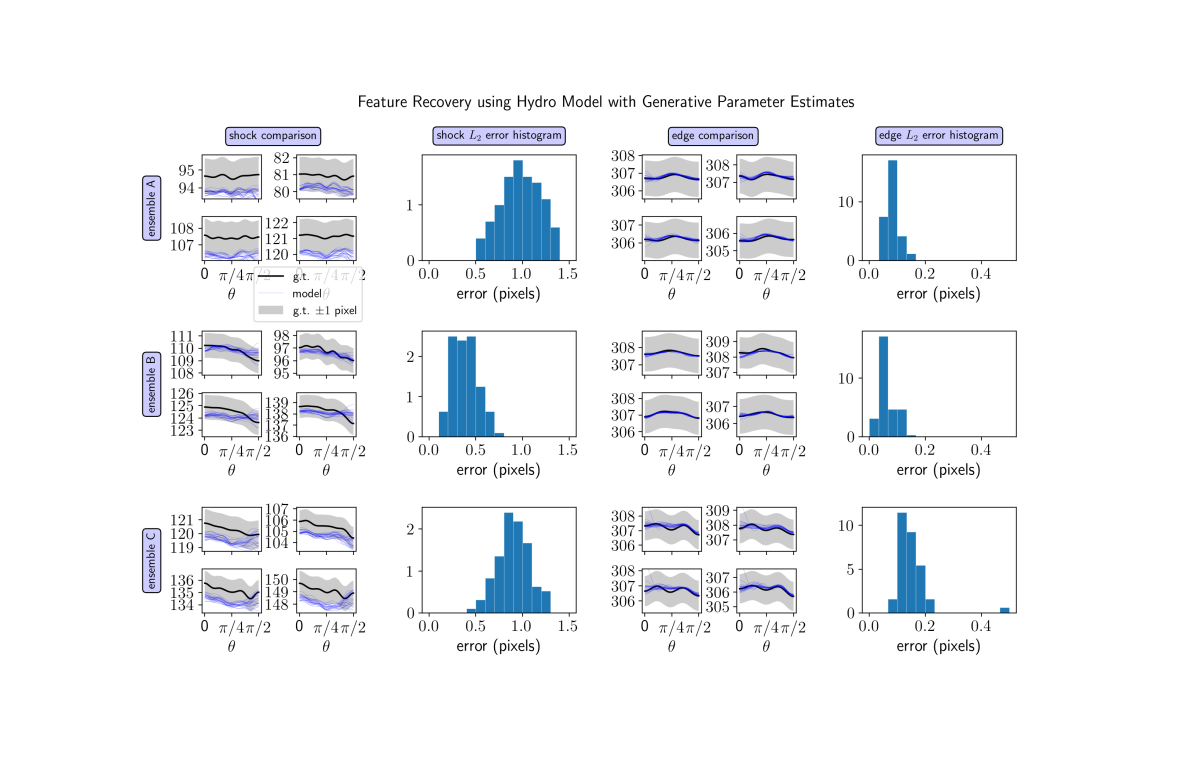
Figure 9: Comparison between three ground truth features (black lines) and ensembles of features (blue lines) obtained through using estimated parameters in a hydrodynamics code. For each ensemble along the rows, this plot shows the comparison of the shock features, histogram of shock $L_{2}$ errors, comparison of edge features, and histogram of edge $L_{2}$ errors. Each feature comparison plot displays four quadrants corresponding to times $n=25,30,35,40$.

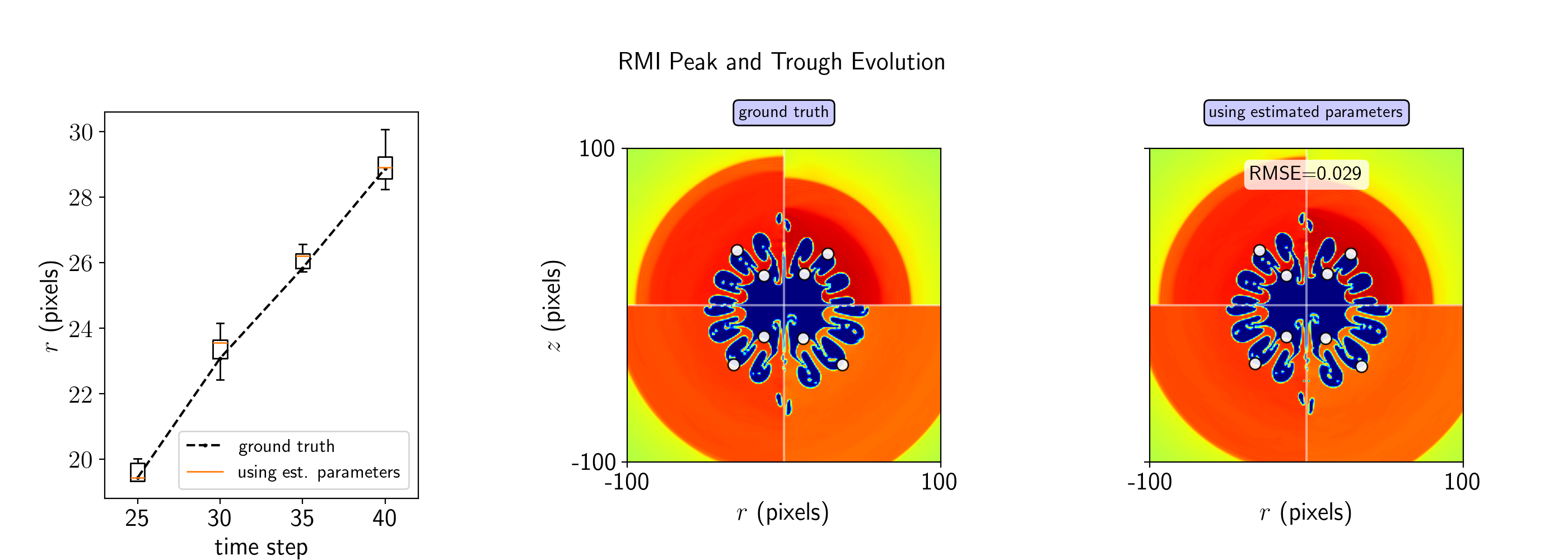
Figure 10: Example using estimated parameters of ensemble A in Figure 8 to predict peak-to-trough evolution of the RMI. Left: evolution of the maximum RMI peak-to-trough radial distance for the ground truth and estimated parameters. Each density field displays four quadrants corresponding to time steps $25,30,35,40$. Middle and right: density fields and identified peak and trough points of the RMI (white markers) for the ground truth field and field obtained using estimated parameters.

Next we explore the impact of model mismatch for our parameter estimation problem. In our study, we chose to use Mie-Grüneison (MG) as a guiding EOS model for our parameter estimation network. However there will always be model mismatch and uncertainty when comparing to experimental data or with simulations utilizing alternative models. In order to study the effect of model mismatch, we generate two sets of density time series using different EOS models - one using the Tillotson (TLN) EOS model [76] and one using the Sesame (SES) EOS model [77]. For each series, we extract features corresponding to the time frames $\{25,30,35,40\}$ and input them into our network to predict corresponding MG parameters and initial conditions. Figure 11 shows comparisons between the ground truth density field and shock and edge features for both the TLN EOS and SES EOS and the corresponding reconstructed density fields and and shock and edge features reconstructed using estimated parameters for the MG EOS model. For the TLN EOS, both the density field and shock and edge features are reconstructed to a reasonable accuracy. However, while the material interface edge is captured accurately for the SES EOS, large errors are present for the density field and shock. For both the TLN and SES EOS, the RMI topology predicted using the MG EOS is qualitatively similar to the ground truth RMI topology. Errors in feature and density consistency due to model mismatch arise from two modalities. First, the guiding EOS model on which parameter estimates are based on must be sufficiently expansive to approximate the unknown EOS model. Second, the features produced by the unknown EOS model must be adequately represented in the training data used to optimize the ML model. It is not surprising that our model is able to able to perform better on simulations produced using the TLN EOS. The MG and TLN EOS models are both globally described by a single equation, while the SES is a tabular model that interpolates multiple local models in different areas of the thermodynamic phase space. Additionally, the features for the simulation using the SES model are outliers compared to the features used in training.

Figure 11: Comparison between density fields and shock and edge features produced using the (a) Tillotson EOS and (b) Sesame EOS and the corresponding density fields and shock and edge features reconstructed using estimated parameters for the Mie-Grüneison EOS model. Predicted shock and edge features are denoted by dotted blue lines and the ground truth features are denoted by black lines with a surrounding gray region depicting an error bar of $\pm$1 pixels.

4 Discussion

In this paper, we demonstrate a new machine learning (ML)-based approach for recovering initial conditions and material parameters in ICF capsule implosions that utilizes hydrodynamic features, such as the outgoing shock profile and outer material edge, that are robustly identifiable in a noisy radiograph. We propose that our method can be used an experimental diagnostic to determine asymmetries in the drive that arise from the Ritchmeyer-Meshkov instability. This experiment can be performed by using an inert gas in lieu of D-T inside of the capsule or by inclusion of a suitable dopant to enable self-generated radiation to be imaged. Our ML approach involves a pipeline consisting of a radiographs-to-features network (R2FNet) and a features-to-parameters network (F2PNet). These networks can be trained independently and later combined during the testing stage. F2PNet also contains a surrogate model for the forward hydrodynamic mapping between parameters-to-features.

Our model problem consists of hydrodynamic simulations of an implosion of a nearly-spherical metallic shell. In our dataset, various equation of state (EOS) parameters and initial conditions on the surface and initial velocity are varied to produce multiple realizations of density field time series. For each simulation, we generated a time series of synthetic radiographs and extracted shock and edge features in the form of cosine harmonic coefficients. Through our results, we demonstrated that our approach is capable of recovering the EOS and initial condition parameters with reasonable accuracy. We also show that the parameter estimates can be successfully used in a surrogate model for the forward problem to accurately estimate the shock and edge features. Additionally, we show that the estimated parameters can be used in a (full-order) hydrodynamic solver to produce density fields with acceptable quantitative accuracy in terms of RMSE and errors in peak-to-trough distance of the RMI surface. We also investigated the ability of the model to estimate parameters when the reference simulation is generated with a different EOS model. Our findings imply that a sufficiently expansive parameter model is capable of representing unknown models.

Appendix A Cosine Coefficients for Inner Surface Perturbation Profile

The coefficients of the cosine harmonic series of the initial inner surface perturbation profile is scaled according to $F_{i}=R_{\rm in}\bar{F}_{i}/8,$ for $i=0,\dots,8$, where $\bar{F}_{0}=8$, $\bar{F}_{5}=\bar{F}_{7}=0$, and the rest of the coefficients are provided by Table 4.

profile	$\bar{F}_{1}$	$\bar{F}_{2}$	$\bar{F}_{3}$	$\bar{F}_{4}$	$\bar{F}_{6}$	$\bar{F}_{8}$
1	0	0	0	0	0	0.08
2	0	0	0	0.08	0	0
3	0	0.08	0	0	0	0
4	0	0	0	0	0	0.075
5	0	0	0	0.075	0	0
6	0	0.075	0	0	0	0
7	0	0.0075	0	0	0.0025	0.065
8	0.0075	0	0.0025	0.065	0	0
9	0.005	0.0657	0	0	0	0
10	0	0	0	0	0	0.06

profile	$\bar{F}_{1}$	$\bar{F}_{2}$	$\bar{F}_{3}$	$\bar{F}_{4}$	$\bar{F}_{6}$	$\bar{F}_{8}$
11	0	0	0	0.06	0	0
12	0	0.06	0	0	0	0
13	0	0	0	0	0	0.055
14	0	0	0	0.055	0	0
15	0	0.055	0	0	0	0
16	0	0.0075	0	0	0.0025	0.045
17	0.0075	0	0.0025	0.045	0	0
18	0.0051	0.0457	0	0	0	0
19	0	0	0	0.04	0	0
20	0	0.04	0	0	0	0

Table 4: Scaled cosine coefficients for the initial shell profile used for each profile.

Appendix B Radiograph-to-Features Network (R2FNet)

The radiograph-to-features network (R2FNet) is illustrated in Figure 12 and is built entirely from convolutions and fully connected linear layers. The first component of the architecture is a convolutional encoder which compresses the series of radiographs from their large ambient dimension to a much smaller latent dimension. The downsampling blocks used in this architecture are identical to the residual blocks used in [78], and are very similar to those found in BigGAN [79]. The network input consists of the four radiographs stacked together so that each timestep is represented by one input channel. The first downsampling block then increases the channel dimension to 64. Each further downsampling block adds an additional 64 channels, and all the downsampling blocks reduce the spatial dimensions by a factor of 2. In the downsampling blocks, the first 3${\times}$3 convolution increases the number of channels. Both networks use 7 downsampling blocks. The outputs of the encoder are then flattened into a vector. Subsequently, there are 3 linear layers - the first of which reduces the dimension by a factor of 16, the second maintains this dimension, and the final layer outputs the parameter predictions.

Radiograph-to-Features Network (R2FNet)

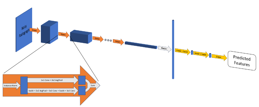
Figure 12: Diagram depicting the radiograph-to-features network (R2FNet). The input is a sequence of noisy radiographs and the output is a corresponding sequence of predicted shock and edge features.

Because the cosine harmonic coefficients of the features of interest have very different absolute scales, they are normalized before being used as targets for training the network. We apply z-score normalization to each coefficient by subtracting its population mean and dividing by its population standard deviation. The loss function used for training is a combination of the mean squared error of the predicted (normalized) coefficients and the mean squared error of the radius of the shock and radius of the edge, sampled on a grid of 500 equally spaced angles $\theta\in[0,\pi/2)$. The R2FNet is optimized using Adam [80], with a learning rate of $10^{-5}$, and a batch size of 8 using eight NVIDIA GeForce RTX 2080 Ti GPUs. The R2FNet achieved its minimum validation loss after approximately 8 hours.

Appendix C Features-to-Parameters Network (F2PNet)

Our features-to-parameters network (F2PNet) combines ideas from the conditional variational autoencoder (cVAE) [81, 82, 83] and the transformer [84], for estimating initial condition (IC) and EOS parameters based on observed outgoing shock and outer edge features. The F2PNet architecture is summarized by Figure 13. F2PNet consists of a forward model, which is a surrogate model for the hydrodynamics operator mapping parameters to features, and a generative parameter estimator, which represents the decoder of a cVAE. For all network inputs and outputs, each EOS parameter and IC parameter are linearly scaled to lie in the range $[0,1]$ and each shock feature is scaled according to its corresponding mean and standard deviation in the training set.

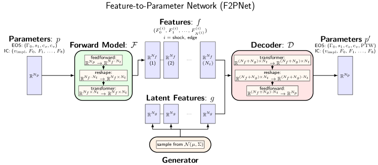
Figure 13: Diagram depicting the features-to-parameters network (F2PNet). The EOS and IC parameters represent the input to the forward model and output of the decoder. The late time shock and edge features are outputs of the encoder. The late time shock and edge features and the latent features randomly sampled from the generator are used as inputs to the decoder.

Consider parameters, $p\in\mathbb{R}^{N_{p}}$, late-time shock and edge features at $N_{t}$ times, $f\in\mathbb{R}^{N_{f}\times N_{t}}$, and generator features, $g\in\mathbb{R}^{N_{g}\times N_{t}}$. The forward model, $\mathcal{F}$, represents a surrogate forward model, predicting late-time shock and edge features from parameters. The first layer is a fully-connected feedforward neural network which outputs data that is reshaped into $\mathbb{R}^{N_{f}\times N_{t}}$. A transformer network, based on [84], is then applied to obtain late-time shock and edge features. The generator draws vectors $g\in\mathbb{R}^{N_{f}\cdot N_{t}}$ from the probability distribution $\mathcal{N}(\mu,\Sigma)$, where $\mu\in\mathbb{R}^{N_{f}\cdot N_{t}}$ and $\Sigma\in\mathbb{R}^{(N_{g}\cdot N_{t})\times(Ng\cdot Nt)}$ are learned parameters. The decoder, $\mathcal{D}$, performs the parameter estimation task given the late-time shock and edge features and randomly generated features. The first layer is a transformer network which outputs data in a shape $\mathbb{R}^{N_{t}\times(N_{f}+N_{g})}$. After reshaping, a fully-connected feedforward neural network is then applied to obtain the parameters.

The model architecture weights are trained using a loss of the form $\mathcal{L}=\mathcal{L}_{\rm decoder}+\mathcal{L}_{\rm forward}+\mathcal{L}_{\rm consistency}+\mathcal{L}_{\rm KL},$ where

$$\mathcal{L}_{\rm decoder}=\frac{1}{N_{d}}\sum_{i=1}^{N_{d}}\|\mathcal{D}(f_{i};g_{i})-p_{i}\|^{2},\quad\mathcal{L}_{\rm forward}=\frac{1}{N_{d}}\sum_{i=1}^{N_{d}}L_{2}(\mathcal{F}(p_{i}),f_{i})^{2},\quad\mathcal{L}_{\rm consistency}=\frac{\alpha}{N_{d}}\sum_{i=1}^{N_{d}}L_{2}(\mathcal{F}(\mathcal{D}(f_{i};g_{i})),f_{i}),$$

and $\mathcal{L}_{\rm KL}=D_{\rm KL}\left(\mathcal{N}(\mu,\Sigma)\;\|\;\mathcal{N}(0,I)\right)$. $\mathcal{L}_{\rm decoder}$ represents the mean squared error between the decoder’s prediction of parameters and the ground truth, $\mathcal{L}_{\rm forward}$ represents the squared $L_{2}$ error between the shock and edge curves defined by the forward model’s prediction of feature coefficients and that of the ground truth, $\mathcal{L}_{\rm consistency}$ represents a self-consistency loss using the same error metric as $\mathcal{L}_{\rm forward}$, but instead using the shock and edge curves reconstructed by applying the forward model to the decoder’s parameter estimates of the ground truth features, and $\mathcal{L}_{\rm KL}$ is the KL divergence between the generator probability distribution and a standard Gaussian distribution. The combination of $\mathcal{L}_{\rm decoder}$ and $\mathcal{L}_{\rm KL}$ represents the traditional VAE loss [81] while the addition of $\mathcal{L}_{\rm forward}$ and $\mathcal{L}_{\rm consistency}$ encourages accuracy and consistency of the forward model. In our study, we first pre-train the architecture without the self-consistency term ($\alpha=0$) to obtain a reasonable initial set of weights for the encoder and decoder, then later perform a second round of training using all of the terms ($\alpha=1$).

In summary, F2PNet combines the strengths of the transformer and conditional variational autoencoder to estimate parameters from temporal sequences of shock and edge features. The transformer provides the ability to capture long range temporal dependencies. Results are presented for an architecture that uses two transformer blocks in the encoder and decoder, each with 8 heads, $H=8$, a latent dimension of $k=64$, and a feedforward neural network with inner dimension 2048 and $\tanh$ activation functions. The feedforward neural networks in the encoder and decoder each have two layers with a hidden dimension of 200.

In our study, we also investigated the use of different network architectures, including networks without attention mechanisms. We discovered that applying attention greatly improves the prediction accuracy of the parameters and therefore we chose to make this a key component of F2PNet. Additionally, we investigated a probabilistic neural network, which models the posterior as a multivariate Gaussian distribution. However, since the posterior is generally a complex probability distribution, we decided to pursue a VAE-based architecture, which is capable of representing non-Gaussian distributions.

Author contributions statement

D.A.S, E.B., M.K., B.S.S., and B.N. conceived the parameter estimation approach. O.K. developed the feature extraction algorithm. D.A.S., E.B., and B.N. conducted the approach. D.A.S., E.B., M.K., and B.S.S. analyzed the results. All authors reviewed the manuscript.

Competing interests

The authors declare no competing interests.

References

- [1] Gittings, M. et al. The rage radiation-hydrodynamic code. \JournalTitleComputational Science & Discovery 1, 015005 (2008).
- [2] Fryxell, B. et al. Flash: An adaptive mesh hydrodynamics code for modeling astrophysical thermonuclear flashes. \JournalTitleThe Astrophysical Journal Supplement Series 131, 273 (2000).
- [3] Marinak, M., Haan, S., Dittrich, T., Tipton, R. & Zimmerman, G. A comparison of three-dimensional multimode hydrodynamic instability growth on various national ignition facility capsule designs with hydra simulations. \JournalTitlePhysics of Plasmas 5, 1125–1132 (1998).
- [4] Zimmerman, G., Kershaw, D., Bailey, D. & Harte, J. Lasnex code for inertial confinement fusion. Tech. Rep., California Univ. (1977).
- [5] Keller, D. et al. Draco—a new multidimensional hydrocode. In APS Division of Plasma Physics Meeting Abstracts, vol. 41, BP1–39 (1999).
- [6] Haines, B. M. et al. The development of a high-resolution eulerian radiation-hydrodynamics simulation capability for laser-driven hohlraums. \JournalTitlePhysics of Plasmas 29 (2022).
- [7] McGlaun, J. M., Thompson, S. & Elrick, M. Cth: A three-dimensional shock wave physics code. \JournalTitleInternational Journal of Impact Engineering 10, 351–360 (1990).
- [8] Weseloh, W. N. Pagosa: a multi-dimensional, multi-material parallel hydrodynamics code for material flow and deformation (u). Tech. Rep., Los Alamos National Laboratory (LANL), Los Alamos, NM (United States) (2011).
- [9] Summers, R., Wong, M., Boucheron, E. & Weatherby, J. Alegra–a massively parallel h-adaptive code for solid dynamics. Tech. Rep., Sandia National Lab.(SNL-NM), Albuquerque, NM (United States) (1997).
- [10] Abu-Shawareb, H. et al. Lawson criterion for ignition exceeded in an inertial fusion experiment. \JournalTitlePhysical review letters 129, 075001 (2022).
- [11] Weber, C. et al. Improving ICF implosion performance with alternative capsule supports. \JournalTitlePhysics of Plasmas 24 (2017).
- [12] Gaffney, J. et al. A review of equation-of-state models for inertial confinement fusion materials. \JournalTitleHigh Energy Density Physics 28, 7–24 (2018).
- [13] Lindl, J. Icf: recent achievements and perspectives. \JournalTitleIl Nuovo Cimento A (1965-1970) 106, 1467–1487 (1993).
- [14] Rosen, M. The physics of radiation driven icf hohlraums. Tech. Rep., Lawrence Livermore National Lab. (1995).
- [15] Lee, S. et al. Effects of parametric uncertainty on multi-scale model predictions of shock response of a pressed energetic material. \JournalTitleJournal of applied physics 125 (2019).
- [16] Rosen, M. D. The physics issues that determine inertial confinement fusion target gain and driver requirements: A tutorial. \JournalTitlePhysics of Plasmas 6, 1690–1699 (1999).
- [17] Thomas, V. A. & Kares, R. J. Drive asymmetry and the origin of turbulence in an icf implosion. \JournalTitlePhysical review letters 109, 075004 (2012).
- [18] Barker, L. & Hollenbach, R. Laser interferometer for measuring high velocities of any reflecting surface. \JournalTitleJournal of Applied Physics 43, 4669–4675 (1972).
- [19] Malone, R. M. et al. Overview of the line-imaging visar diagnostic at the national ignition facility (nif). In International Optical Design Conference, ThA5 (Optica Publishing Group, 2006).
- [20] Celliers, P. et al. Line-imaging velocimeter for shock diagnostics at the omega laser facility. \JournalTitleReview of scientific instruments 75, 4916–4929 (2004).
- [21] McCoy, C. A. & Knudson, M. D. Lagrangian technique to calculate window interface velocity from shock velocity measurements: Application for quartz windows. \JournalTitleJournal of Applied Physics 122 (2017).
- [22] Ahrens, T. J., Gust, W. & Royce, E. Material strength effect in the shock compression of alumina. \JournalTitleJournal of Applied Physics 39, 4610–4616 (1968).
- [23] Asay, J. & Lipkin, J. A self-consistent technique for estimating the dynamic yield strength of a shock-loaded material. \JournalTitleJournal of Applied Physics 49, 4242–4247 (1978).
- [24] Lipkin, J. & Asay, J. Reshock and release of shock-compressed 6061-t6 aluminum. \JournalTitleJournal of applied physics 48, 182–189 (1977).
- [25] Brown, J., Alexander, C., Asay, J., Vogler, T. & Ding, J. Extracting strength from high pressure ramp-release experiments. \JournalTitleJournal of Applied Physics 114 (2013).
- [26] Barnes, J. F., Blewett, P. J., McQueen, R. G., Meyer, K. A. & Venable, D. Taylor instability in solids. \JournalTitleJournal of Applied Physics 45, 727–732 (1974).
- [27] Colvin, J., Legrand, M., Remington, B., Schurtz, G. & Weber, S. A model for instability growth in accelerated solid metals. \JournalTitleJournal of applied physics 93, 5287–5301 (2003).
- [28] Barton, N. R. et al. A multiscale strength model for extreme loading conditions. \JournalTitleJournal of applied physics 109 (2011).
- [29] Smith, R. et al. High strain-rate plastic flow in al and fe. \JournalTitleJournal of Applied Physics 110 (2011).
- [30] Piriz, A. R., Cela, J. L., Tahir, N. A. & Hoffmann, D. H. Richtmyer-meshkov instability in elastic-plastic media. \JournalTitlePhysical Review E 78, 056401 (2008).
- [31] Piriz, A., Cela, J. L. & Tahir, N. Richtmyer–meshkov instability as a tool for evaluating material strength under extreme conditions. \JournalTitleNuclear Instruments and Methods in Physics Research Section A: Accelerators, Spectrometers, Detectors and Associated Equipment 606, 139–141 (2009).
- [32] Dimonte, G. et al. Use of the richtmyer-meshkov instability to infer yield stress at high-energy densities. \JournalTitlePhysical review letters 107, 264502 (2011).
- [33] Buttler, W. et al. Unstable richtmyer–meshkov growth of solid and liquid metals in vacuum. \JournalTitleJournal of Fluid Mechanics 703, 60–84 (2012).
- [34] Ortega, A. L., Lombardini, M., Pullin, D. & Meiron, D. Numerical simulations of the richtmyer-meshkov instability in solid-vacuum interfaces using calibrated plasticity laws. \JournalTitlePhysical Review E 89, 033018 (2014).
- [35] Mikaelian, K. O. Shock-induced interface instability in viscous fluids and metals. \JournalTitlePhysical Review E 87, 031003 (2013).
- [36] Plohr, J. N. & Plohr, B. J. Linearized analysis of richtmyer–meshkov flow for elastic materials. \JournalTitleJournal of Fluid Mechanics 537, 55–89 (2005).
- [37] Prime, M. B. et al. Using richtmyer–meshkov instabilities to estimate metal strength at very high rates. In Dynamic Behavior of Materials, Volume 1: Proceedings of the 2015 Annual Conference on Experimental and Applied Mechanics, 191–197 (Springer, 2016).
- [38] Thomas, V. A. & Kares, R. J. Drive asymmetry, turbulence and ignition failure in high convergence icf implosions. Tech. Rep., Los Alamos National Laboratory (LANL), Los Alamos, NM (United States) (2013).
- [39] Weber, C. et al. Mixing in icf implosions on the national ignition facility caused by the fill-tube. \JournalTitlePhysics of Plasmas 27 (2020).
- [40] Delorme, B. Experimental study of the initial conditions of the rayleigh-taylor instability at the ablation front in inertial confinement fusion. Tech. Rep., Universite de Bordeaux (2015).
- [41] Zhou, Y. et al. Turbulent mixing and transition criteria of flows induced by hydrodynamic instabilities. \JournalTitlePhysics of Plasmas 26 (2019).
- [42] Proano, E. S. & Rollin, B. Toward a better understanding of hydrodynamic instabilities in inertial fusion approaches. In 53rd AIAA/SAE/ASEE Joint Propulsion Conference, 4676 (2017).
- [43] Schaeffer, D. B. et al. Proton imaging of high-energy-density laboratory plasmas. \JournalTitleReviews of Modern Physics 95, 045007 (2023).
- [44] Strobl, M. et al. Advances in neutron radiography and tomography. \JournalTitleJournal of Physics D: Applied Physics 42, 243001 (2009).
- [45] Kozioziemski, B., Bachmann, B., Do, A. & Tommasini, R. X-ray imaging methods for high-energy density physics applications. \JournalTitleReview of Scientific Instruments 94 (2023).
- [46] Endo, T. et al. Dynamic behavior of rippled shock waves and subsequently induced areal-density-perturbation growth in laser-irradiated foils. \JournalTitlePhysical review letters 74, 3608 (1995).
- [47] Serino, D. A., Klasky, M. L., Nadiga, B. T., Xu, X. & Wilcox, T. Reconstructing richtmyer-meshkov instabilities from noisy radiographs using low dimensional features and attention-based neural networks. \JournalTitleOpt. Express 32, 43366–43386, DOI: 10.1364/OE.538495 (2024).
- [48] Zhai, Z., Zou, L., Wu, Q. & Luo, X. Review of experimental richtmyer–meshkov instability in shock tube: from simple to complex. \JournalTitleProceedings of the Institution of Mechanical Engineers, Part C: Journal of Mechanical Engineering Science 232, 2830–2849 (2018).
- [49] Yager-Elorriaga, D. A. et al. Studying the richtmyer–meshkov instability in convergent geometry under high energy density conditions using the decel platform. \JournalTitlePhysics of Plasmas 29 (2022).
- [50] Do, A. et al. High spatial resolution and contrast radiography of hydrodynamic instabilities at the national ignition facility. \JournalTitlePhysics of Plasmas 29 (2022).
- [51] Si, T., Long, T., Zhai, Z. & Luo, X. Experimental investigation of cylindrical converging shock waves interacting with a polygonal heavy gas cylinder. \JournalTitleJournal of Fluid Mechanics 784, 225–251 (2015).
- [52] Rupert, V. Shock-interface interaction: current research on the Richtmyer-Meshkov problem. In Shock Waves: Proceedings of the 18th International Symposium on Shock Waves, Held at Sendai, Japan 21–26 July 1991, 83–94 (Springer, 1992).
- [53] Brouillette, M. The Richtmyer-Meshkov instability. \JournalTitleAnnual Review of Fluid Mechanics 34, 445–468 (2002).
- [54] Zhou, Y. et al. Rayleigh–Taylor and Richtmyer–Meshkov instabilities: A journey through scales. \JournalTitlePhysica D: Nonlinear Phenomena 423, 132838 (2021).
- [55] Leinov, E. et al. Experimental and numerical investigation of the Richtmyer–Meshkov instability under re-shock conditions. \JournalTitleJournal of Fluid Mechanics 626, 449–475 (2009).
- [56] Holmes, R. L. et al. Richtmyer–Meshkov instability growth: experiment, simulation and theory. \JournalTitleJournal of Fluid Mechanics 389, 55–79 (1999).
- [57] Zhou, Y. Rayleigh–Taylor and Richtmyer–Meshkov instability induced flow, turbulence, and mixing. II. \JournalTitlePhysics Reports 723, 1–160 (2017).
- [58] Zhang, Q. & Graham, M. J. A numerical study of Richtmyer–Meshkov instability driven by cylindrical shocks. \JournalTitlePhysics of Fluids 10, 974–992 (1998).
- [59] Hossain, M. et al. High-precision inversion of dynamic radiography using hydrodynamic features. \JournalTitleOptics Express 30, 14432–14452 (2022).
- [60] Bello-Maldonado, P. D., Kolev, T. V., Rieben, R. N. & Tomov, V. Z. A matrix-free hyperviscosity formulation for high-order ale hydrodynamics. \JournalTitleComputers & Fluids 205, 104577 (2020).
- [61] Serino, D. A., Klasky, M., Burby, J. W. & Schei, J. L. Density reconstruction from noisy radiographs using an attention-based transformer network. In Optica Imaging Congress (3D, COSI, DH, FLatOptics, IS, pcAOP), JW2A.4 (Optica Publishing Group, 2023).
- [62] Nadiga, B. T. & Klasky, M. L. Degeneracy and deterministic/probabilistic inversions of radiographic data. LA-UR-23-25917 (2023). Sponsor: USDOE National Nuclear Security Administration (NNSA) ; USDOE ; LDRD.
- [63] Le Pape, S. et al. Observation of a reflected shock in an indirectly driven spherical implosion at the national ignition facility. \JournalTitlePhysical Review Letters 112, 225002 (2014).
- [64] Asch, M., Bocquet, M. & Nodet, M. Data assimilation: methods, algorithms, and applications (SIAM, 2016).
- [65] Smith, D. R. Variational methods in optimization (Courier Corporation, 1998).
- [66] Cai, Z., Chen, J. & Liu, M. Least-squares relu neural network (lsnn) method for scalar nonlinear hyperbolic conservation law. \JournalTitleApplied Numerical Mathematics 174, 163–176 (2022).
- [67] Biegler, L. T., Ghattas, O., Heinkenschloss, M. & van Bloemen Waanders, B. Large-scale pde-constrained optimization: an introduction. In Large-scale PDE-constrained optimization, 3–13 (Springer, 2003).
- [68] Tran, B. K., Southworth, B. S. & Leok, M. On properties of adjoint systems for evolutionary pdes. \JournalTitleJournal of Nonlinear Science 34, 95 (2024).
- [69] Raissi, M., Perdikaris, P. & Karniadakis, G. E. Physics-informed neural networks: A deep learning framework for solving forward and inverse problems involving nonlinear partial differential equations. \JournalTitleJournal of Computational physics 378, 686–707 (2019).
- [70] Cuomo, S. et al. Scientific machine learning through physics–informed neural networks: Where we are and what’s next. \JournalTitleJournal of Scientific Computing 92, 88 (2022).
- [71] Gautam, S. et al. Learning robust features for scatter removal and reconstruction in dynamic icf x-ray tomography. \JournalTitlearXiv preprint arXiv:2408.12766 (2024).
- [72] Merritt, E. C. et al. Experimental study of energy transfer in double shell implosions. \JournalTitlePhysics of Plasmas 26, 052702, DOI: 10.1063/1.5086674 (2019). https://pubs.aip.org/aip/pop/article-pdf/doi/10.1063/1.5086674/15643290/052702_1_online.pdf.
- [73] Hertel, E. S. Jr. & Kerley, G. I. CTH Reference Manual: The Equation of State Package. report SAND98-0947, Sandia National Laboratories (1998).
- [74] van Aarle, W. et al. The ASTRA toolbox: A platform for advanced algorithm development in electron tomography. \JournalTitleUltramicroscopy 157, 35–47, DOI: https://doi.org/10.1016/j.ultramic.2015.05.002 (2015).
- [75] Trujillo-Pino, A., Krissian, K., Alemán-Flores, M. & Santana-Cedrés, D. Accurate subpixel edge location based on partial area effect. \JournalTitleImage and Vision Computing 31, 72–90, DOI: https://doi.org/10.1016/j.imavis.2012.10.005 (2013).
- [76] Tillotson, J. H. Metallic equations of state for hypervelocity impact. \JournalTitleGeneral Atomic Report GA-3216. 1962. Technical Report 3216 (1962).
- [77] Johnson, J. The sesame database. Tech. Rep. LA-UR-94-1451, Los Alamos National Lab.(LANL), Los Alamos, NM (United States) (1994).
- [78] Whang, J. et al. Deblurring via stochastic refinement. In 2022 IEEE/CVF Conference on Computer Vision and Pattern Recognition (CVPR), 16272–16282, DOI: 10.1109/CVPR52688.2022.01581 (2022).
- [79] Brock, A., Donahue, J. & Simonyan, K. Large scale gan training for high fidelity natural image synthesis (2019). 1809.11096.
- [80] Kingma, D. P. & Ba, J. Adam: A method for stochastic optimization (2017). 1412.6980.
- [81] Kingma, D. P. & Welling, M. Auto-encoding variational Bayes. \JournalTitleCoRR abs/1312.6114 (2013).
- [82] Cinelli, L. P., Marins, M. A., Da Silva, E. A. B. & Netto, S. L. Variational methods for machine learning with applications to deep networks (Springer, 2021).
- [83] Kingma, D. P., Mohamed, S., Jimenez Rezende, D. & Welling, M. Semi-supervised learning with deep generative models. \JournalTitleAdvances in Neural Information Processing Systems 27 (2014).
- [84] Vaswani, A. et al. Attention is all you need. In Guyon, I. et al. (eds.) Advances in Neural Information Processing Systems, vol. 30 (Curran Associates, Inc., 2017).
Acknowledgements
This work was supported by the Laboratory Directed Research and Development program of Los Alamos National Laboratory under project number 20230068DR.