A matrix-free interior point continuous trajectory for linearly constrained convex programming
Abstract
Interior point methods for solving linearly constrained convex programming involve a variable projection matrix at each iteration to deal with the linear constraints. This matrix often becomes ill-conditioned near the boundary of the feasible region that results in wrong search directions and extra computational cost. A matrix-free interior point augmented Lagrangian continuous trajectory is therefore proposed and studied for linearly constrained convex programming. A closely related ordinary differential equation (ODE) system is formulated. In this ODE system, the variable projection matrix is no longer needed. By only assuming the existence of an optimal solution, we show that, starting from any interior feasible point, (i) the interior point augmented Lagrangian continuous trajectory is convergent; and (ii) the limit point is indeed an optimal solution of the original optimization problem. Moreover, with the addition of the strictly complementarity condition, we show that the associated Lagrange multiplier converges to an optimal solution of the Lagrangian dual problem. Based on the studied ODE system, several possible search directions for discrete algorithms are proposed and discussed.
1 Introduction
Consider the following linearly constrained convex programming problem
where , , is convex and twice continuously differentiable, is an by matrix with full row rank. As a blanket assumption, we assume that the optimal value for problem (1) is finite and attainable. In addition, the following notations are used in this paper:
The Lagrangian function associated with (1) is defined for every by
and the Lagrangian dual problem associated with (1) is
where .
In interior point methods, the linear constraint is maintained at each iteration, which means that an linear system is generally involved. For example, in the primal affine scaling algorithm [10] for problem (1) with , a projection matrix where is used at each iteration. However, if is very large, then the inverse of the matrix could be quite expensive. In addition, as moves to the boundary of , the matrix could become ill-conditioned. This paper focuses on avoiding this possible ill-conditioning problem caused by the linear constraints for problem (1). Our strategy is to only maintain the positivity of while relaxing the equality constraint . This can be accomplished by combining the traditional interior point methods with the augmented Lagrangian method. We call this new method the matrix-free interior point augmented Lagrangian method. Much attention will be paid to the trajectory of this method, which is actually the solution of an ordinary differential equation (ODE) system.
In particular, we are interested in the continuous solution trajectory of the following ODE system
| (1) |
where
Let us explain where the ODE system (1) comes from. Problem (1) can be written equivalently as
where is the indicator function of defined as
Then the Lagrangian function associated with problem (1) is defined for every as
and the augmented Lagrangian function associated with problem (1) is defined for every as
| (2) |
where is a parameter. To solve problem (1), the augmented Lagrangian method can be used. The augmented Lagrangian method was first proposed by Hestenes [12] and Powell [20]. Since then researchers have studied the augmented Lagrangian method in many different ways. For example, in [23, 24], the augmented Lagrangian method and the proximal point method were studied by Rockafellar, and its convergence rate was obtained. In [31], the exponential method of multipliers, which operates like the usual augmented Lagrangian method except that it uses an exponential penalty function in place of the usual quadratic, was analyzed by Tseng and Bertsekas. In [13], the augmented Lagrangian methods and proximal point methods for convex optimization were considered by Iusem, and by using the generalized distances (Bregman distances and divergences), the generalized proximal point methods and the generalized augmented Lagrangian methods were proposed and studied. In [2], the augmented Lagrangian methods with general lower-level constraints were considered by Andreani , and the global convergence was obtained by using the constant positive linear dependence constraint qualification. In [27], the augmented Lagrangian method for nonlinear semidefinite programming was studied by Sun , and the linear convergence rate was obtained under the constraint nondegeneracy condition and the strong second-order sufficient condition. Zhao [37] considered a Newton-CG augmented Lagrangian method for solving semidefinite programming problems from the perspective of approximate semismooth Newton methods, and the convergence rate was analyzed by characterizing the Lipschitz continuity of the corresponding solution mapping at the origin. However, the method in [37] may encounter numerical difficulty for degenerate semidefinite programming problems. In order to tackle this numerical difficulty, Yang [35] employed a majorized semismooth Newton-CG augmented Lagrangian method coupled with a convergent 3-block alternating direction method of multipliers introduced by Sun [28]. In [11], a new splitting version of the augmented Lagrangian method with full Jacobian decomposition for separable convex programming was proposed by He , and the worst-case convergence rate measured by the iteration complexity in both the ergodic and nonergodic senses was obtained.
Applying the augmented Lagrangian method to problem (1), from any initial point , for we have the following iteration scheme
Step 1. Compute
Step 2. Compute
where is the step size. In Step 1, we need to minimize a convex function over . There are many methods to solve this subproblem. One of them is the interior point method. Particularly, we can use a first-order interior point method which is extended directly from the method in [32]. In [32], Tseng proposed a first-order interior point method for linearly constrained smooth optimization which unifies and extends the first-order affine scaling method and the replicator dynamics method (see [4]) for standard quadratic programming. Notice that the method in [32] cannot be applied to the subproblem in Step 1 directly except in problem (1). However, we can just replace with in for to handle this, and the resulting search direction has the same form as in the ODE system (1) (we restrict ). In fact, if , the direction in the ODE system (1) is the first-order affine scaling direction. The affine scaling algorithm was first introduced by Dikin [8] in 1967. Since then many researchers have studied the affine scaling algorithm in many different ways. For instance, the affine scaling algorithm in linear programming was studied by Dikin [9], Saigal [25], Tseng and Luo [33], Tsuchiya [34], and so on. The affine scaling continuous trajectory was also studied for linear programming, for example, by Adler and Monteiro [1], Liao [14], Megiddo and Shub [17], Monteiro [18]. For convex quadratic programming and more general convex programming, the affine scaling algorithm was studied by Gonzaga and Carlos [10], Monteiro and Tsuchiya [19], Sun [29, 30], Tseng [32], Ye and Tse [36]. The affine scaling algorithm for convex semidefinite programming was studied by Qian [21]. Since this interior point method for the subproblem in Step 1 is an iterative method, in each iteration of the augmented Lagrangian method, can be updated several times and may be updated only once. Hence we may wonder at each iteration of the augmented Lagrangian method, whether could be only updated once. This is part of the motivation of this paper, and the ODE system (1) is exactly the continuous realization of this idea.
For simplicity, in what follows, denotes the 2-norm. stands for the class of th order continuously differentiable functions. Unless otherwise specified, denotes the th component of a vector , and denotes the identity matrix, the dimension of is clear from the context. For any index subset , we denote as the vector composed of those components of indexed by , and denote as the submatrix of composed by choosing the indexed rows and columns in .
The rest of this paper is organized as follows. First, a potential function for the ODE system (1) is introduced in Section 2. Furthermore, it is verified that the ODE system (1) has a unique solution in . With the help of this potential function, in Section 3, we prove that every accumulation point of the continuous trajectory of the ODE system (1) is an optimal solution for problem (1). In Section 4, we show the strong convergence of the continuous trajectory and verify that the limiting point has the maximal number of the positive components in among the optimal solutions. Then with the addition of the strictly complementarity condition, we show that the associated Lagrange multiplier converges to an optimal solution of the Lagrangian dual problem (1). In Section 5, two numerical examples are provided to show the performance of the solution trajectory of the ODE system (1). Several possible search directions for discrete algorithms which are derived from the ODE system (1) are discussed briefly in Section 6. Finally, some concluding remarks are drawn in Section 7.
2 Properties of the solution trajectory of the ODE system (1)
The following assumptions are made throughout this paper.
Assumption 2.1.
There exists a point such that is the optimal value of problem (1).
Assumption 2.2.
on .
Assumption 2.3.
The matrix has full row rank .
Theorem 2.4.
For the ODE system (1), there exists a unique solution with a maximal existence interval , in addition, for on the existence interval.
Proof.
By Assumption 2.2, the right-hand side of the ODE system (1) is locally Lipschitz continuous on . From Theorem IV.1.2 in [5], there exists a unique solution for the ODE system (1) on the maximal existence interval , for some or such that . Since , for on the existence interval. The proof is completed. ∎
Later in this section, it will be shown that (Theorem 2.9). To simplify the presentation, in the remaining of this paper, (or ) and will be replaced by (or ) and , respectively, whenever no confusion would occur.
The next three lemmas lay the foundation for our potential function which will be introduced in (4). Lemmas 2.6 and 2.7 are Lemmas 10 and 11 in [22], respectively.
Lemma 2.5.
(see [6]) Suppose is differentiable (i.e., its gradient exists at each point in ). Then is convex if and only if is convex and
| (3) |
holds for all , .
Proof.
See Section 3.1.3 in [6]. ∎
Lemma 2.6.
Let be any positive constant. Then for any scalar , and if and only if . Furthermore, as or .
Lemma 2.7.
Let be any positive constant and . Then for any scalar , and if and only if . Furthermore, as or .
Next we introduce a potential function for the ODE system (1). With the help of this potential function, the boundedness of the optimal solution set is no longer needed in the convergence proof of the ODE system (1). Instead, only the weaker Assumption 2.1 is needed. In 1983, Losert and Akin [15] introduced a kind of potential function for both the discrete and continuous dynamical systems in a classical model of population genetics. Their potential function can be extended for our purpose. In [22], a similar potential function is also used for the study of the generalized central paths for problem (1). In order to define our potential function, we first introduce some notations. For any , and . Obviously, for any , and . Then the potential function for the ODE system (1) can be defined as
| (4) |
where
| if | (5) | ||||
| if | (7) | ||||
| (9) | |||||
and is the variable, is the parameter.
Theorem 2.8.
Let be the solution of the ODE system (1) on the maximal existence interval . Then is bounded on .
Proof.
We can choose the in Assumption 2.1. Then there exist a and a such that satisfies the following KKT conditions for problem (1)
| (10) |
Hence the convex function attains the minimum at which implies
| (11) |
Since , we can define as follows
| (12) |
From Theorem 2.4, is well defined on , and from Lemma 2.5 and (11) we have
which indicates that
| (13) |
From Lemmas 2.6 and 2.7, we know that for if or , we must have . Hence from (13), must be bounded on . ∎
Theorem 2.9.
Let the maximal existence interval of the solution of the ODE system (1) be . Then .
Proof.
Assume . From Theorem 2.8, we know that there exists an such that and for all . Furthermore, from Assumption 2.2, we know that there exists an such that for every , we have
| (14) |
and for any , , we have
| (15) |
For any , from inequalities (14), (15), and , we know that (without loss of generality we assume )
| (16) |
furthermore, is continuous on , and it is not hard to see that exists. We denote this limit as . Evidently . According to the Extension Theorem in 2.5, [3], we know that the solution will go to the boundary of the open set . But because of the hypothesis, , and is bounded, so there must exist at least one such that . From inequality (14), we know that if ,
Integrating the above inequality, we have for every
Since as , as , but . This is a contradiction. Thus and the proof is completed. ∎
3 Optimality of the cluster point(s)
From Theorem 2.8, we know that the limit set is nonempty. In this section, we will show that for any , is an optimal solution for problem (1). First we need the following lemma.
Lemma 3.1.
(Barbalat’s Lemma [26]) If the differentiable function has a finite limit as , and is uniformly continuous, then as .
Theorem 3.2.
For any , is an optimal solution for problem (1).
Proof.
We can choose the in Assumption 2.1, and as the corresponding Lagrange multiplier for constraint (see the proof of Theorem 2.8). Note that when , we have . From Lemmas 2.6 and 2.7, it is easy to see that for all . Therefore, for all , is bounded below. This along with the fact that implies that has a finite limit as .
From Theorem 2.8, we know that the solution of the ODE system (1) is contained in the bounded closed set for some . From the proof of Theorem 2.8, we have
| (17) |
which is continuously differentiable with respect to according to Assumption 2.2, hence when is compact, there must exist a constant such that
Using inequality (16), we have
thus is uniformly continuous with respect to . Hence from Barbalat’s Lemma and (17), we have that
| (18) |
For any , from the definition of , we know that there exists a sequence with as such that and as . Then since is continuous at , from (3), (11), and (18), we have
which implies and
Furthermore, Theorem 2.4 and the definition of , for . Hence is an optimal solution for problem (1). Thus the theorem is proved. ∎
4 Convergence of the solution trajectory of the ODE system (1)
Now, it comes to the key results of the paper. To simplify the notation, we define
| (19) |
and , where is the solution of the ODE system (1). Let and . Theorem 4.3 below shows that converges as , and under the strict complementarity condition, converges to an optimal solution of the dual problem (1). First we need the weak convergence of the ODE system (1) and the following lemma.
Lemma 4.1.
([16]) Let be a twice continuously differentiable convex function. If is constant on a convex set then is constant on .
Theorem 4.2.
Proof.
From (2), we can define and from (19) we have
| (20) |
Furthermore, from Theorems 2.8 and 3.2, it is not hard to see that
| (21) |
From Theorem 2.8, we know that the solution of the ODE system (1) is contained in a bounded closed set for some . Moreover, is continuously differentiable with respect to according to Assumption 2.2, hence when is in this bounded closed set, there must exist a constant such that
thus is uniformly continuous with respect to . Hence from (20), (21), and Barbalat’s Lemma, we have that
Furthermore, from Theorem 3.2, we know
hence
which implies
Thus the proof is completed. ∎
Theorem 4.3.
Let be the solution of the ODE system (1). Then the following results hold.
-
(a)
For any , , and any optimal solution of problem (1), .
-
(b)
converges to an optimal solution of problem (1) which has the maximal number of positive components in among all optimal solutions.
-
(c)
If there exists a pair of primal and dual optimal solutions satisfying the strict complementarity, then converges to an optimal solution of problem (1).
Proof.
(a) It should be noticed that from (10), is an optimal solution of problem (1). Hence the optimal solution set of problem (1) is not empty. Assume . We can define as follows
| (22) |
for any . From Theorems 2.4 and 2.9, is well defined on , and from Lemma 2.5 and Theorem 3.2 we have
Since is an optimal solution of problem (1), we have
which implies
Furthermore is bounded below by zero, hence exists. Since , there exists with such that
This along with (22) and (4) implies
| (23) |
Similarly, since and , we have
which contradicts with (23). Hence the hypothesis is not true and we have . Similarly, we can show that and thus .
(b) Without loss of generality, we assume that the optimal solution in Assumption 2.1 has the maximal number of positive components in among all optimal solutions. For any , from Theorem 3.2, we know that is an optimal solution of problem (1). From (12), (13), and Lemmas 2.6 and 2.7, it is easy to see that for each , is bounded below by some positive constant . So from Theorem 3.2, must have the maximal number of positive components in among all optimal solutions and , .
where
| (28) |
From Lemmas 2.6, 2.7, and (4), it is straightforward to see that for any and . For any , we also have , hence is continuous at . Then since exists from the proof of (a), we have that
this along with (a) implies that . Thus .
(c) Without loss of generality, we assume that and satisfy the strict complementarity. According to Assumption 2.2 and Lemma 4.1, is constant on the optimal solution set of problem (1). For , if , then converges to by (a). In this case, from , (10), and (b), we have that converges to . Obviously, is an optimal solution of problem (1) by (10).
Now we consider the case of . For , from Theorem 4.2 and , we know that for or , . By the strict complementarity, for , , thus there exists a such that for we have that for with
Moreover, for or , for . Let . Then from , we have . Hence for , also satisfies the KKT conditions (10), which implies that is an optimal solution of problem (1) for . If there is a such that , then there exists a 2-dimensional plane passing through , , and . On this 2-dimensional plane, we denote the circle centered at with radius by and denote the circle centered at with radius by . Then from (a), we know that should be on the two circles and simultaneously. But this is impossible since the two circles and have only one point in common. Hence and converges as . This along with (b), we have that converges to .
5 Numerical examples
In this section, we show the performance of the solution trajectory of the ODE system (1) on two examples. The first example is from [22], and has the following form
| (30) |
where and are variables, the optimal solutions are on the -axis , and . For the details of this example, see Section 4 in [22]. The problem (30) is actually a specific instance in [7], where a class of examples are proposed to show that the central path may fail to converge. The problem (30) is a special case of problem (1) with .
We plot the central path and the solution trajectories of the ODE system (1) with different initial points for problem (30). For our solution trajectories, we let , , and . A Matlab solver ode23s is used to compute the trajectories of the ODE system (1). For the central path, a Matlab code provided by Prof. Karas of [7] is used. In Fig. 1 (a), cp represents the central path and sp represents the solution trajectory of the ODE system (1). Both paths have the same initial point . Fig. 1 (b) is just a magnified display of the solution trajectory in Fig. 1 (a). Fig. 2 shows the solution trajectories with different initial points.

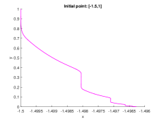
(a) Trajectories of cp and sp (b) Trajectory of sp
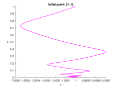
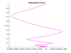
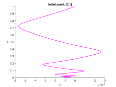
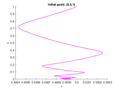
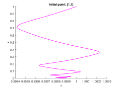
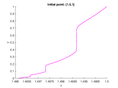
Fig. 1 and Fig. 2 clearly show that for problem (30), the central path is a zig-zag path with large swing, while the solution trajectories of the ODE system (1) do converge.
Next, we show the performance of the solution trajectory of the ODE system (1) and primal (first-order) affine scaling trajectory for the following problem
| (31) |
where , , , and
It is easy to verify that is the unique optimal solution of problem (31), and satisfies the KKT conditions of problem (31) which are equivalent to
This implies that is actually the optimal solution set of the corresponding dual problem.
The primal (first-order) affine scaling trajectory can be characterized by the following ODE system
| (32) |
where , , and needs to satisfy and . We plot the primal affine scaling trajectory and the solution trajectory of the ODE system (1) from Matlab solver ode23s. For the direction in (32), the involved linear system caused by the matrix is solved by left division operator “” in Matlab. For ode23s, the relative error tolerance “RelTol” is set as , and the absolute error tolerance “AbsTol” is set as . For our solution trajectory, we set , , and . In Fig. 3, the magenta trajectories and the blue trajectories represent the coordinate behaviors of the solution trajectory of the ODE system (1) and the primal affine scaling trajectory, respectively. The two green dashed lines show the behaviors of our solution trajectory , and the green line represents , which should converge to according to the definition of . The initial point for the primal affine scaling trajectory is , and the initial point for the solution trajectory of the ODE system (1) is and .
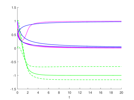
Fig. 3 shows that both the primal affine scaling trajectory and our solution trajectory of the ODE system (1) converge, and our solution trajectory actually converges faster than the primal affine scaling trajectory.
Table 1 lists the results at the end point of the solution trajectory of the ODE system (1) and the primal affine scaling trajectory for various integral intervals . In Table 1, sp represents the solution path of the ODE system (1), and ap represents the primal affine scaling path. means the minimum coordinate value of , and represents the condition number of the matrix (the inverse of is involved in the affine scaling direction) at point for the primal affine scaling trajectory. In Table 1, NaN means that ode23s failed due to the ill-conditioning.
| sp | ap | sp | ap | sp | ap | ap | |
|---|---|---|---|---|---|---|---|
| 10 | 2.7e-2 | 9.7e-2 | 1.6e-3 | 2.5e-12 | 1.5e-2 | 4.9e-2 | 1.2e+3 |
| 5.2e-4 | 1.3e-2 | 3.5e-5 | 4.1e-11 | 2.2e-4 | 6.3e-3 | 7.9e+4 | |
| 5.6e-6 | 1.3e-3 | 4.4e-7 | 2.8e-10 | 2.3e-6 | 6.6e-4 | 7.2e+6 | |
| 5.6e-8 | 1.3e-4 | 5.6e-9 | 1.1e-8 | 2.3e-8 | 6.7e-5 | 7.0e+8 | |
| 5.5e-10 | 1.3e-5 | 1.3e-10 | 5.1e-7 | 2.2e-10 | 6.7e-6 | 7.0e+10 | |
| 5.3e-12 | 1.3e-6 | 7.8e-13 | 2.2e-6 | 2.2e-12 | 6.6e-7 | 7.0e+12 | |
| 4.9e-14 | 1.1e-6 | 4.0e-15 | 2.6e-6 | 2.0e-14 | 8.9e-8 | 5.9e+14 | |
| 4.0e-16 | 1.1e-6 | 5.0e-16 | 2.5e-6 | 1.6e-16 | 7.2e-9 | 3.5e+15 | |
| 4.0e-18 | NaN | 0 | NaN | 1.7e-18 | NaN | NaN | |
Table 1 clearly shows that for the degenerate case where is singular at some point on the boundary of the feasible region, the interior point method could encounter ill-conditioning problem, while our method is matrix-free.
6 Further discussion
In this section, we discuss about the possible search directions and algorithms which derived from the ODE system (1). For the ODE system (1), the simplest implementation way is the explicit Euler scheme. In fact, from any initial point , this algorithm have the forms
| (33) |
and
| (34) |
where is the step size,
and
In order to guarantee the optimality of the algorithm, some line search strategies and restrictions may be needed to decide the step size .
At , some semi-implicit directions can also be generated by the ODE system (1). One possible way is that
where represents the step size. This can be calculated approximately as
which is a new search direction. If we want to follow the particular solution trajectory of the ODE system (1) with the initial point , should move a small along the search direction . However, because of the residual, the point may not be in . Moreover, our purpose is not simulating any particular solution trajectory of the ODE system (1), instead, we aim at finding the limit point of the solution path. Thanks to Theorem 4.3, the limit point of from any initial point is an optimal solution for problem (1). Hence we can do a line search along this search direction, and can be regarded as a positive parameter. This direction involves an inverse of a symmetric positive definite matrix, which needs too many calculations for large scale problems. Hence, in practice, the solution of the corresponding linear equations could be solved approximately.
Another semi-implicit search direction can be generated from the following form
where also represents the step size. Then can be calculated approximately as
Similar to the discussion of the first semi-implicit search direction, can be regarded as a positive parameter and the step size can be decided by a line search.
Now in order to obtain more search directions, we make a division of the index set . Let be nonempty index sets with such that for and . For the explicit Euler scheme of the ODE system (1), the iteration (33) can be divided to sequential steps according to the index division, which means that moves to sequentially from to at each iteration. Then when we calculate , we may use instead of for , and this generates a new iteration. But there comes a question: how to decide the step size? One possible solving way is to calculate the step size for each respectively. The may be different from each other, which seems unreasonable since then the search direction at each iteration can not be derived from the ODE system (1) directly, but this can be solved by bring in a weighted vector for the ODE system (1). Actually if we replace in the ODE system (1) by
where is a diagonal matrix with if , then corresponding to this weighted ODE system, the new iteration can be derived from the following semi-implicit form
It is evident that with step size equals to one, the above form generates the new iteration. Furthermore, it is easy to see that by similar proofs, the same results of the ODE system (1) hold for this weighted ODE system.
For the division of index set , there are many other search directions which can be generated from the ODE system (1). Here we enumerate two more possible implementations. One possible implementation way is the following semi-implicit form
Similarly, the can be calculated approximately as
| (35) | |||||
for , and can be regarded as a positive parameter and the step size can be decided by a line search. It is interesting to see that for this implementation, the iteration for can also be divided to sequential steps. Hence similar to the discussion before, when we calculate , we can use instead of for , and decide the step size by the line search respectively. However, this new search direction in this new iteration scheme seems not be able to be derived from the ODE system (1), since each may be not equal to . Hence in this situation, we may regard this new iteration scheme as a partially updated algorithm in the sense that at each iteration, for the in (35), we only move one along , and proceed this process from to sequentially and then loop.
In the above discussion, we only considered the . For , we can use or . Different choice can lead to different algorithms. It should be noticed that, some of the above search directions involve the inverse of the matrix or the block sub-matrix, but the condition number of them can be controlled by the restriction of the hyperparameters. In this section, we only discuss the possible search directions for discrete algorithms briefly, and the study of these algorithms can be the future research.
7 Concluding remarks
Ill-conditioning subproblems arise in the computation of many interior point algorithms for linearly constrained convex programming problems. In this paper, we have developed a matrix-free interior point augmented Lagrangian continuous trajectory for these problems. This continuous trajectory can be viewed as the solution of the ODE system (1) and only matrix-vector product is required in this ODE system (1). It has been proved that starting from any interior feasible point, this continuous trajectory would always converge to some optimal solution of the original problem. Therefore, a stepping stone is laid for developing a matrix-free numerical scheme to follow this convergent continuous trajectory. In particular, we discuss several possible search directions for discrete algorithms briefly, and further study could be the future research.
References
- [1] Ilan Adler and Renato DC Monteiro. Limiting behavior of the affine scaling continuous trajectories for linear programming problems. Mathematical Programming, 50:29–51, 1991.
- [2] Roberto Andreani, Ernesto G Birgin, José Mario Martínez, and María Laura Schuverdt. On augmented lagrangian methods with general lower-level constraints. SIAM Journal on Optimization, 18(4):1286–1309, 2008.
- [3] Dmitrij V Anosov, Vladimir Igorevich Arnold, and DV Anosov. Dynamical systems I: ordinary differential equations and smooth dynamical systems. Springer, 1988.
- [4] Immanuel M Bomze. Regularity versus degeneracy in dynamics, games, and optimization: a unified approach to different aspects. SIAM review, 44(3):394–414, 2002.
- [5] Nicolas Bourbaki. Functions of a real variable. Springer Berlin Heidelber, 2004.
- [6] Stephen Boyd and Lieven Vandenberghe. Convex optimization. Cambridge university press, 2004.
- [7] J Charles Gilbert, Clovis C Gonzaga, and Elizabeth Karas. Examples of ill-behaved central paths in convex optimization. Mathematical programming, 103(1):63–94, 2005.
- [8] II Dikin. Iterative solution of problems of linear and quadratic programming. In Doklady Akademii Nauk, volume 174, pages 747–748. Russian Academy of Sciences, 1967.
- [9] II Dikin. On the convergence of an iterative process. In Upravlyaemye Sistemy, volume 12, pages 54–60, 1974.
- [10] Clovis C Gonzaga and Luiz A Carlos. A primal affine scaling algorithm for linearly constrained convex programs. preprint, 1990.
- [11] Bingsheng He, Liusheng Hou, and Xiaoming Yuan. On full jacobian decomposition of the augmented lagrangian method for separable convex programming. SIAM Journal on Optimization, 25(4):2274–2312, 2015.
- [12] Magnus R Hestenes. Multiplier and gradient methods. Journal of optimization theory and applications, 4(5):303–320, 1969.
- [13] Alfredo N Iusem. Augmented lagrangian methods and proximal point methods for convex optimization. Investigación Operativa, 8(11-49):7, 1999.
- [14] Li-Zhi Liao. A study of the dual affine scaling continuous trajectories for linear programming. Journal of Optimization Theory and Applications, 163:548–568, 2014.
- [15] Viktor Losert and Ethen Akin. Dynamics of games and genes: Discrete versus continuous time. Journal of Mathematical Biology, 17:241–251, 1983.
- [16] Olvi L Mangasarian. A simple characterization of solution sets of convex programs. Operations Research Letters, 7(1):21–26, 1988.
- [17] N Megiddo and M Shub. “Boundary behavior of interior point algorithms for linear programming,” ibm research report rj5319, 1986.
- [18] Renato DC Monteiro. Convergence and boundary behavior of the projective scaling trajectories for linear programming. Mathematics of Operations Research, 16(4):842–858, 1991.
- [19] Renato DC Monteiro and Takashi Tsuchiya. Global convergence of the affine scaling algorithm for convex quadratic programming. SIAM Journal on Optimization, 8(1):26–58, 1998.
- [20] Michael JD Powell. A method for nonlinear constraints in minimization problems. Optimization, pages 283–298, 1969.
- [21] Xun Qian, Li-Zhi Liao, and Jie Sun. A strategy of global convergence for the affine scaling algorithm for convex semidefinite programming. Mathematical Programming, 179(1):1–19, 2020.
- [22] Xun Qian, Li-Zhi Liao, Jie Sun, and Hong Zhu. The convergent generalized central paths for linearly constrained convex programming. SIAM Journal on Optimization, 28(2):1183–1204, 2018.
- [23] R Tyrrell Rockafellar. Augmented lagrangians and applications of the proximal point algorithm in convex programming. Mathematics of operations research, 1(2):97–116, 1976.
- [24] R Tyrrell Rockafellar. Monotone operators and the proximal point algorithm. SIAM journal on control and optimization, 14(5):877–898, 1976.
- [25] Romesh Saigal. A simple proof of a primal affine scaling method. Annals of Operations Research, 62(1):303–324, 1996.
- [26] Jean-Jacques E Slotine. Applied nonlinear control. PRENTICE-HALL google schola, 2:1123–1131, 1991.
- [27] Defeng Sun, Jie Sun, and Liwei Zhang. The rate of convergence of the augmented lagrangian method for nonlinear semidefinite programming. Mathematical Programming, 114(2):349–391, 2008.
- [28] Defeng Sun, Kim-Chuan Toh, and Liuqin Yang. A convergent proximal alternating direction method of multipliers for conic programming with 4-block constraints. arXiv preprint arXiv:1404.5378, 2014.
- [29] Jie Sun. A convergence proof for an affine-scaling algorithm for convex quadratic programming without nondegeneracy assumptions. Mathematical Programming, 60(1):69–79, 1993.
- [30] Jie Sun. A convergence analysis for a convex version of dikin’s algorithm. Annals of Operations Research, 62:357–374, 1996.
- [31] Paul Tseng and Dimitri P Bertsekas. On the convergence of the exponential multiplier method for convex programming. Mathematical programming, 60(1):1–19, 1993.
- [32] Paul Tseng, Immanuel M Bomze, and Werner Schachinger. A first-order interior-point method for linearly constrained smooth optimization. Mathematical Programming, 127:399–424, 2011.
- [33] Paul Tseng and Zhi-Quan Luo. On the convergence of the affine-scaling algorithm. Mathematical Programming, 56(1):301–319, 1992.
- [34] Takashi Tsuchiya. Global convergence of the affine scaling methods for degenerate linear programming problems. Mathematical Programming, 52:377–404, 1991.
- [35] Liuqin Yang, Defeng Sun, and Kim-Chuan Toh. Sdpnal+: a majorized semismooth newton-cg augmented lagrangian method for semidefinite programming with nonnegative constraints. Mathematical Programming Computation, 7(3):331–366, 2015.
- [36] Yinyu Ye and Edison Tse. An extension of karmarkar’s projective algorithm for convex quadratic programming. Mathematical programming, 44:157–179, 1989.
- [37] Xin-Yuan Zhao, Defeng Sun, and Kim-Chuan Toh. A newton-cg augmented lagrangian method for semidefinite programming. SIAM Journal on Optimization, 20(4):1737–1765, 2010.