On convergence of Thurston’s iteration for transcendental entire functions with infinite post-singular set
Abstract.
Given an entire function with finitely many singular values, one can construct a quasiregular function by post-composing with a quasiconformal map equal to identity on some open set . It might happen that the -orbits of all singular values of are eventually contained in . The goal of this article is to investigate properties of Thurston’s pull-back map associated to such , especially in the case when is post-singularly infinite, that is, when acts on an infinite-dimensional Teichmüller space .
The main result yields sufficient conditions for existence of a -invariant set such that its projection to the subspace of associated to marked points in is bounded in the Teichmüller metric, while the projection to the subspace associated to the marked points in (generally there are infinitely many) is a small perturbation of identity. The notion of a fat spider is defined and used as a dynamically meaningful way define coordinates in the Teichmüller space.
The notion of asymptotic area property for entire functions is introduced. Roughly, it requires that the complement of logarithmic tracts in degenerates fast as shrinks. A corollary of the main result is that for a finite order entire function, if the degeneration is fast enough and singular values of escape fast, then is Thurston equivalent to an entire function.
1. Introduction
In complex dynamics, one investigates the long term behaviour of sequences of iterations , of a holomorphic function . In transcendental dynamics, the main focus is on the case when is a transcendental entire function, i.e., an entire function which is not a polynomial. Elementary examples are , , , where is a polynomial, etc.
The set of singular values of , denoted , is defined as the closure of the set of all critical or asymptotic values. In this article we mainly restrict to the case when is of finite type, that is, . Dynamical behaviour of singular values defines to a big extent the global dynamics of . One extreme of this behaviour is when all singular values escape (i.e., converge to under the iteration of ). As an analogue from polynomial dynamics one could think of the complement of the Mandelbrot set, which is the set of escaping parameters. Each point in the complement of the Mandelbrot set corresponds to a quadratic polynomial for which the critical value escapes. The mode of this escape is described by two parameters: potential and external angle. By analogy one can ask: how exactly the singular set of an entire function can escape? And more generally: which post-singularly infinite behaviour appears for entire functions?
A global strategy to answer such questions is the following.
-
(1)
Choose some meaningful (for the class of functions under consideration) dynamical behaviour (e.g., in terms of orbit portraits, speed of escape, combinatorics, etc.)
-
(2)
Construct a (topological) map whose “singular values” model the desired dynamical behaviour.
-
(3)
Decide if this map is “equivalent” to an entire map.
This article aims to address the third item in this list for some types of post-singular dynamics including escaping dynamics.
More precisely, let be an entire function of finite type and be a quasiconformal map equal to identity in some neighbourhood of . Consider the composition . The singular values of are naturally defined as the images of the singular values of under . This map is a quasiregular (rather than just topological) model from the second item of the list above. Denote by the union of singular orbits (under ) and assume that there is a Riemann domain containing , such that
-
(1)
,
-
(2)
is forward invariant,
-
(3)
every singular orbit has a non-empty intersection with .
Thus, models the post-singular dynamics which is absorbed by and eventually controlled by . It turns out that in many natural cases the “parameter space” of contains an entire function with “the same” dynamical behaviour of singular values.
On the formal level “the sameness” is described as
Definition 1.1 (Thurston equivalence).
We say that is Thurston equivalent to an entire map if there exist two homeomorphisms such that
-
(1)
on ,
-
(2)
the following diagram commutes
-
(3)
is isotopic to relative to .
Following [EL], we say that an entire function belongs to the parameter space of if there exist quasiconformal homeomorphisms such that . It is easy to see that for a finite type function , if is Thurston equivalent to an entire function , then belongs to the parameter space of . Thus, for the holomorphic realization of the model we must look in the parameter space of .
Note that the model map is quasiregular rather than just topological. On one hand, this is a strong restriction, on the other, in [Re] it is shown in much bigger generality that given two functions from the same parameter space, they are quasiconformally conjugate on the set points staying under iterations in some domain . This gives a hope that most of the models represented within the parameter space can be obtained with help of the construction above.
1.1. Asymptotic area property
Let us introduce the class of entire functions we are going to work with. It is defined by asymptotic area property which could be considered as a somewhat stronger version of the area property introduced in [ER]. A related discussion also appears in [EL].
Let be a transcendental entire function of bounded type. For a compact contained in denote and let
that is, is the cylindrical measure of the set , which could be either finite or infinite. Then, according to the definition in [ER], has area property if for every . However, we are interested in a parametrized version of this integral.
Let be an open bounded set, denote and consider the parametrized integral
Definition 1.2 (Asymptotic area property).
We say that has asymptotic area property (AAP) relative to an open set if
We say that has AAP if it has AAP relative to every open set .
Elementary examples of a function with are , , , for a non-constant polynomial .
The asymptotic area property does not imply the area property: as grows, on one hand, becomes bigger, on the other, cylindrical measure of is included starting from a bigger radius.
We will be mostly interested in the case when tends to as tends to . Let us restrict to it. The asymptotics of depends on the initial choice of the domain . However, in many cases (e.g. for finite type functions with bounded degrees of critical points) one can find a function such that for every , . If this is the case, we say that is a degeneration function for .
Next theorem is a corollary of the main result.
Theorem 1.3 (Singular values with fast speed of escape).
Let be a transcendental entire function of finite type having degeneration function for some , and satisfying the inequality for some constant and all big enough (it holds, in particular, for functions of finite order).
For a quasiconformal map equal to identity near , consider the quasiregular map with singular values and corresponding escaping singular orbits such that:
-
(1)
for some and all big enough, ,
-
(2)
the set , where is cylindrical distance, has a positive lower bound.
Then is Thurston equivalent to an entire function.
By cylindrical distance we understand the distance with respect to the conformal metric . It is defined on and coincides with the Euclidean metric in the logarithmic coordinates.
Note that generically the escaping points tend to escape even faster than in item (see e.g. [RRRS, Lemma 3.1]).
1.2. Infinite-dimensional Thurston theory
Given a quasiregular function , we need to be able to decide whether it is equivalent to an entire function. A general approach for answering such types of questions was developed by Thurston and Douady–Hubbard [DH, H2]: Thurston’s topological characterization of rational functions is a criterion allowing to decide whether a post-critically finite branched covering of the -sphere is equivalent to a rational map. The branched covering defines naturally a “pull-back map ” acting on the Teichmüller space of the complement to the post-critical set. The branched covering is Thurston equivalent to a rational map if and only if has a fixed point. It is easy to see that does not increase Teichmüller distances, which makes plausible existence of fixed points. Thus, the question of Thurston equivalence is reduced to the study of the properties of .
There are two major directions for the generalization of this classical result. The first one is by considering other classes of functions, for instance, transcendental entire and meromorphic functions. In this regard one should mention [HSS], generalizing the theory for the exponential family, and the PhD thesis of Sergey Shemyakov [She], encompassing more general families of entire functions. Another direction is by considering post-critically infinite dynamics. The corresponding generalization for hyperbolic rational functions is treated in [CT].
A subject of separate interest lies in the intersection of the two directions. The case of transcendental entire functions with the post-singular set which is infinite “near ” (e.g., if all singular values escape) cannot be reduced to the two cases above. The reason is that is an essential singularity for transcendental entire functions, hence one cannot apply the techniques from the rational case. Markus Förster shows in his PhD thesis [F] that every “mode” of escape in the exponential family can be realized as the post-singular “mode”. The approach is using pull-backs of “spiders” with infinitely many “legs” which can be interpreted as a version of Thurston’s pull-back map . These techniques were generalized in [Bo1, Bo2, Bo3] for the families where is a polynomial. An important feature of the construction is that one is considering the pull-back map defined on the infinite-dimensional Teichmüller space (of the complement of the set of marked points). Unfortunately, there are only weaker versions of Teichmüller’s theorems in this setup, hence different techniques are required (than in finite-dimensional case). We also note the in [CT], the authors reduce the infinite-dimensional setting to the finite-dimensional using quasiconformal surgery, hence apparently one cannot reproduce this approach in a neighbourhood of an essential singularity.
Following the strategy of [F, Bo1, Bo2, Bo3], in order to prove existence of a fixed point of , two major ingredients are required:
-
•
a -invariant pre-compact subset of the corresponding Teichmüller space,
-
•
should be strictly contracting on .
The two conditions imply existence of a fixed point by an elementary argument.
By strict contraction we mean that decreases the distances, but not necessarily with a uniform contraction factor smaller than one (hence one cannot apply the Banach Fixed Point Theorem). To address this problem we might use [Bo1, Lemma 4.1] saying that if the -images of two asymptotically conformal points are also asymptotically conformal (see Subsection 3.3 for the definition), then decreases the distances between them.
Thus, the set must contain only asymptotically conformal points. This is one of the reasons to consider entire functions satisfying asymptotic area property. For instance, think about such so that its singular orbits are very sparse near , e.g., separated by round annuli around the origin with moduli tending to . Then, if we apply to a Teichmüller equivalence class of a homeomorphism which is “nearly identity” near , after pulling-back its Beltrami coefficient via and integrating it, due to Teichmüller-Wittich theorem 2.12, we obtain a Teichmüller equivalence class of homeomorphism which is also “nearly identity” near . Roughly speaking, the main difficulty in the construction of is to arrange that the former neighbourhood of is contained inside of the latter. This would imply the invariance of under .
The main result of the present article is Theorem 7.5. At this point, we provide only a heuristic description of the result, for more details see Section 7.
-
***
Invariant set. Let be a finite type function and be a neighbourhood of . Assume that is such that the singular orbits of are absorbed by in the sense described above and be a domain such that .
If the first points belonging to on each post-singular orbit are -distant from each other (in cylindrical metric), the set is separated from the boundary of by an annulus of big enough modulus, and, for some universal constant and a constant depending on and , the product is small enough, then the corresponding extended Teichmüller space contains a -invariant set such that:
-
(1)
if we “forget” the post-singular points in , then the corresponding projection of to the finite-dimensional Teichmüller space is bounded in the Teichmüller metric;
-
(2)
every Teichmüller equivalence class in contains a homeomorphism which is -distant from identity on (in the -cylindrical metric).
-
(1)
By an extended Teichmüller space space we understand the set of Teichmüller equivalence classes after we relax the requirement for every homotopy class to contain a quasiconformal map. The reason for doing this is that in the infinite-dimensional setup, a point in the Teichmüller space and its -image do not necessarily belong to the same Teichmüller space. However, is well-defined as a map on the extended Teichmüller space.
By we denote the total amount of points in the set . In the proof of Theorem 7.5 it will be seen that roughly corresponds to the maximal dilatation of representatives in after “forgetting” the points in . The requirement for the product to be small is a strict way of saying that Thurston’s pull-back of the representative, or, more precisely, of its restriction to , is a quasiconformal map with presumably very big maximal dilatation, but supported on a set of very small area. In this setting, it is possible to prove a special type of Koebe-like distortion bounds and to show that the representative will be uniformly close identity on .
The proof of Theorem 7.5 has three major ingredients depending on the type of marked points.
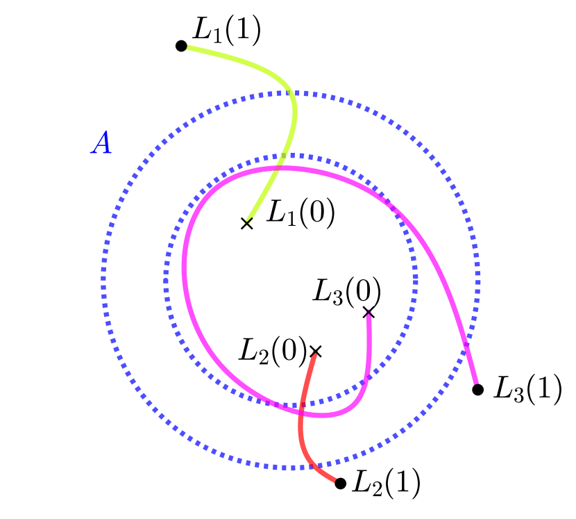
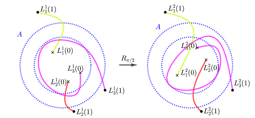
The marked points contained in are controlled with help of Koebe-like estimates obtained in Section 5. To control the behaviour of the marked points in , we define a special structure called fat spider. It has some similarity to the classical spider introduced in [HS] for encoding the combinatorics of post-critically finite polynomials, but the principles of functioning are quite different. First, the “body” of the classical spider is the point while the “body” of a fat spider is a big disk around (hence “fat”). The feet of a fat spider are finitely many marked points in the complement of the body and separated from it by an annulus of some definite modulus. Each feet is connected to the body by a homotopy class of paths (called “legs”) in the complement of marked points. To every leg we associate the maximal dilatation of a quasiconformal map which maps the underlying foot to the body along the leg and (via isotopy) relative to all other feet. Given a homeomorphism equal to identity on the body so that the images of all feet are separated from the body by the same annulus we can consider the push-forward of the spider, in which its legs are just push-forwards of the legs of the initial fat spider. If we also know the maximal dilatation associated to the legs of the pushed-forward spider, we have an estimate on the maximal dilatation of the homeomorpism, see Proposition 6.12. On the other hand, it is not difficult to define a lift (with augmentation) of a spider leg which corresponds to the map and for which it is convenient to compute the corresponding maximal dilatations. Note, that we do not have a standard spider in the sense of [HS], i.e., some invariant structure formed by external rays. Instead the spider legs change on every iteration on both the left and the right hand sides the commutative diagram for .
Finally there should be some ingredient which “glues” these two very different types of storing information about points in the Teichmüller space in order to keep this decomposition invariant under . This ingredient is the property of which we call -regularity of tracts. Roughly, this means the following. Consider some big and two punctured disks around : and , and two logarithmic tracts such that and , and assume that . Then we say that a pair of tracts is -regular if every point belonging to can be mapped to some point of the circle via a -quasiconformal map equal to identity outside of . This property allows to define a dynamically meaningful pull-back of a fat spider. It will be shown that for having finite order the value of can be estimated in terms of . For a more detailed version with marked points see Subsection 6.2.
1.3. Structure of the article
In Section 2 we briefly discuss some properties of entire functions and connections to the cylindrical metric. Afterwards we provide some basic notions from the theory of quasiconformal maps together with a rather lengthy list of statements we are going to use.
In Section 3 we define the (extended) Teichmüller space, introduce formally the -map and discuss its contraction properties. Finally, we prove a few semi-standard statements about different types of quasiconformal representatives in the Teichmüller equivalence classes.
Section 4 is devoted to asymptotic area property. In particular, we investigate dependence of the degeneration function on .
In Section 5 we discuss quasiconformal maps with small “total dilatation per area ratio” and show that locally they can be approximated by identity with the quantitative bounds depending only on the ratio (Proposition 5.3). In the proof of the main result (Theorem 7.5) this allows to control the behaviour of marked points near .
Section 6 consists of three parts. In Subsection 6.1 we introduce the homeomorphisms of a special type, called shifts, and investigate their properties. In Subsection 6.2 we define formally the -regularity and compute bounds for for entire functions of finite order (Proposition 6.9). Finally, in Subsection 6.3 we define fat spiders and show how the maximal dilatation of a homeomorphism can be bounded using the information about the underlying fat spiders (Proposition 6.12).
In Section 7 we first introduce a separating structure. This is in some sense an “environment” we are going to work in. It is needed in order to be able to prove Theorem 7.5 without fixing some particular and for many different types of dynamics altogether. We construct a standard fat spider and introduce the pull-back procedure (of standard spiders) corresponding to . Afterwards, we state and prove Theorem 7.5 and conclude the section with a rather simple Theorem 7.6 allowing to deduce existence of a fixed point for certain settings of Theorem 7.5.
1.4. Acknowledgements
I would like to thank Kevin Pilgrim for the series of fruitful discussions of aspects of Teichmüller theory during his visit to Saarbrücken. I would like to thank Nikolai Prochorov and Dierk Schleicher for their feedback, especially for the discussion related to the parameter spaces of entire functions. Also I would like to express my gratitude to Feliks Przytycki for his support during my stay at IMPAN.
1.5. Notations and agreements
We denote by the complex plane and the Riemann sphere, respectively.
For , we denote by the disk around of radius . If we omit the index , this means that , if we omit the center , this means that .
By we denote the disk with center at , and for , is the right half-plane .
For a subspace of a topological space we denote by its boundary and by the interior of .
For , by we denote the open round annulus between the circles and .
When we say that an isotopy is relative to some set , we imply that this isotopy is constant on . In particular, when it contains the identity map, this means that all maps along the isotopy are equal to identity on .
2. Standard notions and definitions
In this section we assemble definitions and results about transcendental entire functions and quasiconformal maps.
2.1. Logarithmic coordinates and cylindrical metric
We are mainly interested in the class of entire functions of finite type (also called Speiser class or class ) and occasionally we consider the entire functions of bounded type (also called Eremenko-Lyubich class or class ). For the former ones, the singular set is finite, for the latter ones — bounded.
Recall that the set of singular values is defined as the closure of the set of critical and asymptotic values. A critical value is the image of a critical point. We say that is an asymptotic value for if there exists a path such that and . In particular, is always a singular value for . However, when speaking about singular values, we always mean a finite singular value and denote their set by .
By the post-singular set of we understand the closure of the union of forward orbits of singular values (including the singular value itself). Note that very often we need to distinguish between the union of singular orbits (without taking the closure) and . In this case we denote this union using the letter .
For , the logarithmic coordinates are introduced as follows. Let be big enough, so that , and let . Then is a union of unbounded simply-connected connected components called (logarithmic) tracts of . Then the restriction can be lifted via the exponential map. The derived function is called logarithmic transform of and is denoted by .
is defined on the -periodic set of pre-images of tracts (also called tracts) under the exponential. The restriction of to each tract is a conformal map onto the right half-plane .
The logarithmic coordinates are well suited for orbits staying “near ”, in particular, for the escaping points. The most important feature of these coordinates is that for big enough , is expanding, and in a quite strong way [EL, Lemma 1]:
We will not require the explicit inequality in this article, but we will occasionally use the strong expansivity of .
The cylindrical area is defined on by the area element . For , we will denote by the distance between points in the cylindrical metric and call it cylindrical distance. Note that its pull-back under the exponential coincides with the Euclidean metric — we will use this property regularly throughout the article.
2.2. Quasiconformal maps
The most standard references are [A, BF, LV], though the latter one will be used most intensively in this article.
Definition 2.1 (Quadrilateral).
A quadrilateral is a Jordan domain together with a sequence of boundary points called vertices of the quadrilateral. The order of vertices agrees with the positive orientation with respect to . Arcs and are called -sides, arcs and are called -sides.
Every such quadrilateral is conformally equivalent to the unique canonical rectangle with the length of -sides equal to 1. For a quadrilateral , the length of the -sides of the canonical rectangle is called a modulus of and is denoted .
Analogously, every annulus is conformally equivalent to a unique round annulus for some . Then the modulus of is defined as . Note that it is more colloquial to have a factor in front of the logarithm. However, we will follow the convention in [LV].
A maximal dilatation can be defined both in terms of the moduli of quadrilaterals and of the moduli of annuli. The defined objects coincide.
Definition 2.2 (Maximal dilatation).
Let and be planar domains and be an orientation-preserving homeomorphism. The maximal dilatation of is called the number
,
where the supremum is taken over all quadrilaterals (resp. annuli) contained in together with its boundary.
Using we can define quasiconformal maps.
Definition 2.3 (Quasiconformal map).
An orientation-preserving homeomorphism of a plane domain is called quasiconformal if its maximal dilatation is finite. If , then is called -quasiconformal.
The inverse of a -quasiconformal map is also -quasiconformal, while the composition of a -quasiconformal and -quasiconformal map is -quasiconformal.
Quasinconformal maps can also be defined analytically.
Definition 2.4 (Quasiconformal map).
A homeomorphism of a plane domain is quasiconformal if there exists such that
-
(1)
has locally integrable, distributional derivatives and on , and
-
(2)
almost everywhere.
Such is called -quasiconformal, where .
Each quasiconformal map is determined up to a post-composition by a conformal map by its Beltrami coefficient.
Definition 2.5 (Beltrami coefficient).
The function is called the Beltrami coefficient of . It is defined almost everywhere on .
Providing the Beltrami coefficient is almost the same as proiding a quasiconformal map. Consider the Beltrami equation
where the partial derivatives and are defined in the sense of distributions and are locally integrable.
Theorem 2.6 (Measurable Riemann Mapping Theorem [GL]).
The Beltrami equation gives a one-to-one correspondence between the set of quasiconformal homeomorphisms of that fix the points and and the set of measurable complex-valued functions on for which .
We finish this subsection by providing a list of somewhat more advanced statements about quasiconformal maps.
Theorem 2.7 (Theorem 2.1, [McM]).
Any annulus of sufficiently large modulus contains an essential (i.e., separating the boundary components of ) round annulus with .
Lemma 2.8.
[LV, Section I.4.4, Rengel’s inequality] Let be a quadrilateral with (Euclidean) area and be Euclidean distances between its a-sides and b-sides respectively (measured along paths inside of ). Then
The inequality in each case is possible if and only if is a rectangle.
Lemma 2.9.
[LV, Chapter II, inequality (9.1)] Let be a -quasiconformal map such that and for some , . Then
For a quasiconformal map , let .
Lemma 2.10.
Let be a quadrilateral such that its -sides lie on different sides of a horizontal strip of height and let be a quasiconformal map of . Then
Proof.
The proof is the same as for the analogous inequality for rectangles in [LV, Chapter V, Section 6.3]. Following the notation of the book, we have to assign when be longs to the intersection of with the strip, and otherwise. ∎
Lemma 2.11.
[LV, Chapter V, inequality (6.9)] Let be a round annulus around and be a quasiconformal map of . Then
The following result is a part of the Teichmüller-Wittich theorem. In this article, we follow the exposition of [LV]. An alternative proof of the theorem can be found in [Shi]. Another reference for a similar type of results is [Bi].
Theorem 2.12.
[LV, Satz 6.1, Teichmüller–Wittich theorem] Let be a quasiconformal map such that and
Then is complex differentiable (conformal) at .
3. Teichmüller spaces and Thurston’s theory
3.1. Teichmüller spaces
Definition 3.1 (Teichmüller space of ).
For a set , the Teichmüller space of with the marked set is the set of quasiconformal homeomorphisms of modulo post-composition with an affine map and isotopy relative to (or, equivalently, relative to ).
By we denote the set of topological homeomorphisms of modulo post-composition with an affine map and isotopy relative to .
Remark 3.2.
A more standard definition of the Teichmüller space on a Riemann surface involves isotopy relative the ideal boundary rather than the topological boundary. For planar domains the two definitions are equivalent [GL].
Every Teichmüller space is equipped with the Teichmüller metric with respect to which is a complete metric space.
Definition 3.3 (Teichmüller distance).
Let . The Teichmüller distance is defined as
Clearly, is contained in and consists exactly of the equivalence classes containing a quasiconformal map. If is finite, then .
The points belonging to the set are called marked points. Since an isolated point is a removable singularity for a quasiconformal map, our setting agrees with the more colloquial one when one considers the Riemann sphere instead of : the formal difference lies in either “forgetting” about (as we do) or making it a marked point (not having any dynamical meaning later on).
For and , we denote by the projection of to , i.e. the Teichmüller equivalence class is defined as the image of the class under the forgetful map which “forgets” the marked points .
3.2. Setup of Thurston’s iteration
Let be a transcendental entire function of bounded type, be a quasiconformal map and . Further, let be a forward invariant set containing . The most important example for us is when is of finite type and all singular values of escape. In this case the union of the orbits of singular values can be chosen as .
The quasiregular map defines Thurston’s pull-back map
acting on the Teichmüller space , via the following diagram:
More precisely, due to Measurable Riemann Mapping Theorem, applied to the pull-back of the Beltrami coefficient of via , for every quasiconformal map there is another quasiconformal map such that is an entire function. Thus, define . The standard lifting argument shows that is well defined.
Note that according to our definition of we do not consider for an arbitrary topological homeomorphism because, generally speaking, if is infinite, the equivalence class might not contain any single quasiconformal map. If this is the case, there is no Beltrami coefficient to pull-back and integrate. And even if is defined, and might belong to different Teichmüller spaces (see [Bo1, Section 3.3]) which makes it umpossible to use the contracting properties of . However, this setup will still be useful if we restrict to finite type entire functions . Then the domain of definition of can be extended to as follows. Let for some topological homeomorphism . There is a quasiconformal map such that , i.e., a quasiconformal representative of the projection of to . Moreover, there exists an isotopy between and relative to . Thus, to obtain , we first choose some in the usual way and then lift the isotopy starting at . The terminal point will be . The usual lifting argument shows that such prolongation of is well defined and there is a map
Analogously, if are two sets (not necessarily forward invariant) such that and , one can interpret as a map
It will be clear from the context which exactly version of is under consideration.
Fixed points of correspond to the entire functions which are Thurston equivalent to .
Lemma 3.4.
[DH, Proposition 2.3] The quasiregular function is Thurston equivalent to an entire function if and only if has a fixed point.
However, in order to apply the contraction properties and deduce existence of a fixed point we need to act on some Teichmüller space (which is not always the case if is infinite). Very often one can deal with this obstacle by switching to a certain -invariant subset of .
3.3. Strict contraction
It is easy to see that if is contracting on , i.e., for every pair of distinct ,
where is the Teichmüller metric. For proof, one needs to pull-back their composition via one of the entire maps appearing on the right hand side of the Thurston diagrams (either for or ). The maximal dilatation will not increase.
However, this is not enough for deducing existence of a fixed point of and a stronger condition is required. In fact, can be strictly contracting on a particular subset of .
Definition 3.5 (Asymptotically conformal points [GL]).
A point is called asymptotically conformal if for every there is a compact set and a quasiconformal representative such that almost everywhere on .
Consider the quasiregular function constructed in the previous subsection. Then the pull-back map associated to tends to decrease distances between asymptotically conformal points if their -images are asymptotically conformal.
Lemma 3.6 (Strict contraction of ).
Assume that every singular value of is either escaping or strictly pre-periodic. Let be -invariant set containing only asymptotically conformal points.
Then some iterate is strictly contracting on , or, equivalently, if , then
Sketch of proof.
The lemma is a simple upgrade of [Bo1, Lemma 4.1] allowing orbits to merge. We show now what has to be modified by using the notation of [Bo1, Lemma 4.1]. Recall that an entire function has at most one omitted value which is necessarily an asymptotic value. Therefore, if does not contract strictly the distance between and , the quadratic differential cannot have poles associated to marked points not having singular values on its orbits (in particular on marked points belonging to cycles). This means that has finitely many poles and its pull-back coincides with , but the indices of the marked points with an associated pole are decreased by one. This procedure can be repeated at most finitely many times, say (depending only on the orbit portrait): otherwise we obtain an integrable quadratic differential without poles, hence equal to . Thus, we can take . ∎
3.4. Representatives of Teichmüller equivalence classes
We prove a few rather technical statements about existence of a suitable for us representative in Teichmüller equivalence classes. Similar statements are represented in the literature, but often in a slightly different form (e.g., without explicit boundss for the dilatation). Therefore, we provide them in the form suitable for ad hoc application and with proofs.
The lemma below, though elementary, will be used in multiple places throughout the article after trivial modifications (such as for disks of different radii).
Lemma 3.7.
Let be a -quasiconformal map such that and is conformal for some . If , then can be isotoped relative to to a -quasiconformal map so that it is conformal on and .
Analogously, if for some and , then can be isotoped relative to to a -quasiconformal map so that and .
Proof.
Construct an auxiliary isotopy of as follows. On the annulus define , while on let . Then the composition is the desired isotopy between and a -quasiconformal map , which is conformal on .
For the case we might consider the isotopy instead. ∎
Next two lemmas are providing bounds on the maximal dilatation if we isotope a quasiconformal map in a neighbourhood of a point in order to make it either conformal or equal to identity there. It is clear that the constant can be replaced by any other smaller than .
Lemma 3.8 (Conformality near puncture).
Let be a -quasiconformal map such that . Then is isotopic relative to to a -quasiconformal map such that is conformal and .
Proof.
Let : its particular value will be chosen later. Consider a quasiconformal map fixing the origin such that its Beltrami coefficient is equal to in and equal to the Beltrami coefficient of in . Then the map is -quasiconformal and conformal on .
Now, we construct a suitable isotopy of , which is conformal on . Note first that since the modulus of is at least , the image is contained in where . Indeed, if , then (use, for example, [LV, Formula I.6.1] with the Euclidean metric ), hence .
Assume that is chosen in such a way that has hyperbolic diameter (in ) not exceeding , i.e., . Then as in the proof of [Bo1, Lemma 4.2] we see that the quasisymmetry constant of the function is bounded independently of (by following the notation of [Bo1, Lemma 4.2]). It follows from [BF, Proposition 2.28] and the Alexander trick that can be isotoped relative to a quasiconformal map such that and its maximal dilatation is universally bounded.
Restrict to or, equivalently, . Then the composition is conformal on and has maximal dilatation not exceeding , for some universal constant .
Note that , but using Lemma 3.7 we can additionally isotope to a map having the maximal dilatation at most . ∎
Lemma 3.9 (Identity near puncture).
Let be two Riemann domains, be maximal radii so that and be a -quasiconformal map such that . Then is isotopic relative to to a -quasiconformal map such that and .
Sketch of proof.
First, let us prove the lemma for .
After applying Lemma 3.7 and Lemma 3.8 we might assume that is conformal on and has maximal dilatation . Let . From the Grötzsch inequality, . Applying also Lemma 2.9 we obtain
That is, contains a round disk around of a radius . After post-composing with the isotopy from Lemma 3.7, we might assume additionally that contains and has maximal dilatation . The Koebe -Theorem implies that is universally bounded from above and from below. The proof can be concluded by interpolation as in [BF, Proposition 2.28] together with the standard Koebe distortion argument applied to the conformal map (note that the “quasisymmetric” constants are universally bounded on if is close enough to ).
More generally, if are such that , pre- and post-composition of with the respective Riemann maps fixing reduces the problem to the solved case above. On the other hand, for the Riemann maps the derivatives at are universally bounded from above and below, hence one can isotope them to identity on with the universal bound on maximal dilatation. Thus, as in the case of the unit disks, .
Finally, let be arbitrary Riemann domains. Consider the map defined on the rescaled domain. Applying the conclusion of the previous paragraph we see that can be isotoped relative to to a map which is equal to on and has maximal dilatation . This new map can be isotoped to a map equal to identity on and having maximal dilatation . Using Lemma 3.7 and increasing the bounds we might extend the domain on which to . ∎
Next two statements are giving an answer to the following question. Given a Riemann domain with two marked points in it, how big is the maximal dilatation induced by moving one point into another by an isotopy relative to the boundary of the domain?
Lemma 3.10.
Let be an annulus and let points be contained in the bounded component of . Then there exists a -quasiconformal map equal to identity on the unbounded component of such that and .
Proof.
Let be the union of with the bounded component of . Without loss of generality we might assume that is the unit disk and for some . The annulus of the biggest modulus separating and from is the Grötzsch extremal domain (see [LV, Section II.1]). Therefore, we might assume that . Next, after changing coordinates via applying a Möbius transformation we assume that for some . From the central simmetry of one sees that it is enough to apply a half twist exchanging and and leaving the interval invariant, in order to provide a quasiconformal map exchanging and . Most easily this can be done for the round annulus of modulus equal to : direct computation shows that the induced maximal dilatation will be equal to . ∎
The lemma above can be restated in the form which is more convenient for us.
Corollary 3.11.
Let and . Then can be mapped to any other point of by a -quasiconformal map equal to identity on and with .
Proof.
We can restrict to the case when . As in the lemma above, if , then the annulus of maximal modulus in , separating them from is the complement in of the hyperbolic geodesic segment joining to . Thus, this modulus will be the smallest if and , i.e., the hyperbolic distance between them is equal to . After a holomorphic change of coordinates we might assume that and where .
The annulus of the largest modulus separating and from is the Grötzsch extremal domain having modulus (see [LV, Section II.1] for the definition of the function ). From [LV, Section 2.1, Equation (2.7)] and [LV, Section 2.1, Equation (2.11)], converges to a negative constant as . Using the estimate of Lemma 3.10, we obtain the required bound. ∎
We finish this subsection by a short computation needed to bound the maximal number of twists happening under a -quasiconformal automorphism of the thrice punctured sphere. The bound is quite rough, but it will be sufficient for our needs.
Lemma 3.12 (Twist angle in thrice punctured sphere).
Let and be a -quasiconformal homeomorphism isotopic relative to to an -twist of the annulus (in particular, ). Then for some universal constant ,
Proof.
Let be an isotopy relative to such that and . Since the Teichmüller metric on the 4-punctured sphere coincides with the hyperbolic metric, we have to bound from below the length of the geodesic segment in the homotopy class of the curve .
This length is commensurable with the length of the geodesic segment in , hence for some universal constant . Lifting this segment to the right half plane via we obtain a geodesic segment between points with the real parts equal to and the difference between their imaginary parts equal to . Then
and
∎
4. Asymptotic area property
In this section we in more details functions having asymptotic area property (AAP).
Let , be an open bounded set and denote . Consider the function
Recall from the Introduction (Definition 1.2) that has AAP relative to an open set if
and has AAP if it has AAP relative to every open set . It is easy to see from this definition that it is enough to check AAP only for bounded . Further, in the case when has finite type, one can restrict only to ’s being the union of arbitrarily small disjoint disks around singular values.
It is convenient to have some bound for which is independent of . Proposition 4.4 justifies this approach at least in some generality.
Definition 4.1 (Degeneration function).
Let have AAP. We will say that is an (area) degeneration function for if for every open ,
We are mainly interested in the setup when the degeneration function tends to as . Sometimes it is possible to provide a very precise asymptotics for . A particular example should be more enlightening here.
Example 4.2.
The exponential function has AAP with a degeneration function equal to .
Proof.
It is enough to prove the statement for where . If , then is a vertical strip bounded by the straight vertical lines and . Therefore, it is sufficient to prove the bound for .
For , the angular measure of in is equal to . Since is much smaller than and hence much smaller than as , we have . Finally,
∎
Similar computations show that any function where is a non-constant polynomial, as well as and , have degeneration functions equal to while for , it is .
Along with the integral we will need to consider its more general version depending on a parameter :
Clearly, the value of at coincides with the value of at , but computed for the function . It is natural to expect that and have with commensurable degeneration functions. This is indeed the case.
Lemma 4.3.
Let have AAP with respect to . Then for every ,
whenever is big enough.
Proof.
If , then trivially . Thus, we focus on the case .
Denote and fix some such that . Let us switch to the logarithmic coordinates with being some logarithmic transform of . Consider a parametrized nested family of tracts such that and let be the set of all such families modulo vertical translation by . Recall that the pull-back of the cylindrical metric under the exponential map is Euclidean metric and denote by the area of a measurable set inside of the right half-plane . Then we can write
Therefore, in order to prove the lemma, it is enough to show that for big enough (independent on the choice of the family in ), holds the inequality
| (4.1) |
Indeed, after summing up the right hand side of (4.1) over all families in , we obtain
Let us prove the inequality (4.1). By a small abuse of notation we assume that , i.e., is univalent, and for every , consider three horizontal segments , and . Let be the set of all such that has a non-empty intersection with the strip . By making big enough, we might assume that when . Then the length of of is smaller than , hence for every , the curve is contained in . On the other hand, if is much bigger than , due to Koebe distortion theorem applied to and a big disk centered at , the derivatives are uniformly commensurable along every (e.g., up to a multiplier ). This provides the desired bound on the area and finishes the proof of the lemma. ∎
More easily, if has AAP for , then for every , has AAP for , and for big enough , the values computed for do not exceed computed for where are some constants.
If is of finite type, using similar techniques we can prove an even stronger result.
Proposition 4.4 (AAP for finite type functions).
Let be a finite type entire function with bounded degrees of critical points and where ’s are bounded Riemann domains with pairwise disjoint closures.
If has AAP relative to , then it also has AAP relative to any other open set containing all singular values.
Moreover, for big enough and some constants , ,
Sketch of proof.
Choose some pairwise disjoint bounded Riemann domains such that and let be a Riemann map of mapping to . Denote and fix some numbers such that for every singular value , and . Without loss of generality we might assume that and .
In the setting as above we can switch to the “semi-logarithmic coordinates” in a sense that for every , there is a map defined on a disjoint union of Riemann domains. The setup is well-defined because we are only interested in the pre-images (or their parts) of under which are far from the origin. We need to consider cases depending on the type of the branched covering , where is a connected component of . We are going to work with each separately so let us suppress from the indices and locally use the notation .
-
(Regular value)
Let be a conformal map. Then from the Koebe 1/4-theorem and -periodicity of the exponential map follows that is universally bounded. Therefore, due to Koebe distortion theorem, the diameters of are uniformly bounded and the area of is commensurable with the are of . This means that the space in (compared to ) added inside of the regular pre-image domains has area commensurable to the area already included into for some and corresponding to a regular pre-image.
-
(Critical value)
Let be a branched covering of degree with the only critical point . Then there exists a lift of of the form and its inverse is a conformal map of . Since the degrees of critical points are bounded, we can proceed as in the previous case.
-
(Asymptotic value)
Let be a covering of infinite degree. We can switch to the genuine logarithmic coordinates by considering a conformal map defined by the relation . Then, similarly as in the proof of Lemma 4.3, by Koebe distortion argument, the -pre-images of segments have lengths bounded independently of . For the same reason, the area distortion near such segments is bounded, and the claim follows.
∎
Note that generically behaves well under composition of functions. That is, if and have AAP, then it is natural to expect that also has AAP. Indeed, if we switch to the logarithmic coordinates , then the pull-back of the cylindrical measure is the Euclidean measure. So, if the tracts of “fill” almost all space near , their preimage under should “fill” most of the area in the tracts of . For example, a very rough estimate shows that has AAP with magnitude .
5. Koebe-like estimates for quasiconformal maps with small dilatation per area
We will prove two quantitative estimates for the quasiconformal maps possibly having a very big maximal dilatation but supported on a small area. The computations rely heavily on the techniques from the proof of the Teichmüller–Wittich theorem 2.12 as presented in [LV, Chapter V.6].
Lemma 5.1 (Conditional Koebe distortion).
Let be a quasiconformal map such that and
If we restrict to such that for some parameter , then:
-
(1)
for every , is bounded from below by a constant depending only on ;
-
(2)
there exists a radius such that for every , is bounded from above by a constant depending only on .
Moreover, as , the radii can be chosen in such a way that for every ,
where as .
Proof.
From the Teichmüller–Wittich Theorem 2.12, we know that is conformal at , hence after rescaling we may assume that , i.e., as .
Let . From Lemma 2.11, we obtain
| (5.1) |
From Theorem 2.7, if is small enough, there exists a round annulus centered at so that . We may assume that is the maximal such annulus, i.e., its outer radius is equal to and its inner radius to . Due to the conformality at , by making small we have for any initially chosen .
Thus, as the inequality (5.1) rewrites as
which implies that is bounded from below by a constant depending only on (but note that it is also bounded from above by ). This proves the first part of the statement.
Choose (if possible) some such that where is the universal constant from Theorem 2.7. Then from the inequality
we see that , hence there exists a circle centered at and contained in . This means that
The estimate for follows almost immediately from the proof of [LV, Hilfssatz V.6.1] if we upgrade the input data. More precisely, we no longer need the maximal dilatation to estimate the quantity (notation of [LV]). Instead, use the uniform bounds obtained from the first part of the lemma, i.e., for and some constant depending only on . Then it follows from [LV, Chapter V, inequality (6.21)] together with the discussion in the subsequent paragraph, that is smaller than (tending to as ) if where depends only on . Then the required statement can be proved exactly as the first part of the lemma: the universal constant from Theorem 2.7 can be replaced by a constant arbitrarily close to . ∎
Before proving a similar statement for angular distortion, we need a short preparatory lemma. For (a small) , denote by the rectangle and consider the situation when such rectagle is divided into two quadrilaterals by an injective path contained in the interior of except of its endpoints belonging to different vertical sides of . The upper and the lower quadrilaterals are denoted by and , respectively. We assume that the orientation is chosen in such a way the and the horizontal sides of are the corresponding -sides of and .
Lemma 5.2.
Fix some . For every , there exist such that if simultaneously , and , then the path is contained inside of a horizontal strip of height at most .
Proof.
Let us consider the annulus obtained by gluing together with its mirror copy along the vertical sides. Then the union of with its mirror copy is a topological circle dividing into two annuli and , each of them being the quadrilaterals and , respectively, glued with their mirror copies.
Then and , (the relations follow immediately from [LV, Hilfssatz 6.5] after noticing that and have an axis of symmetry). Due to Theorem 2.7, if is big enough (that is, when is small enough), contains a round annulus such that for some universal constant . Then the curve is contained inside of the round annulus between and . However, by superadditivity of modulus,
Therefore
as . Since and are concentric round annuli, the claim follows. ∎
Now, we state and prove a key result that allows us to maintain and reproduce an “invariant structure” in Theorem 7.5. It says, that if the cylindrical integral is small for a quasiconformal map fixing , then this map is predictably close to identity on a neighbourhood of which is independent of the maximal dilatation, and depends only on the value of the integral.
Proposition 5.3 (Distortion of identity).
For every , there exist and a radius , so that the following statement holds.
If is a quasiconformal map such that , and
then for ,
Proof.
The first part of the proposition, about the radial distortion, is already proven in Lemma 5.1. To provide bounds for the angular distortion, let us switch to the logarithmic coordinates. This can be described by the following diagram where by we denote the left half-plane . The map is defined up to a vertical translation by , so we fix some choice of it.
If we denote
in the logarithmic coordinates the integral inequality rewrites as
where , and . Clearly, can be translated vertically without changing . Let us agree that for a curve, the difference between the supremum and the infimum of the imaginary parts of points belonging to the curve is called height of the curve. Thus, in order to prove the proposition, we need to show that for every there exist and such that if and , then for every , the height of is smaller than .
First, given , we show existence of and such that if and , then for at least one . Consider a (very long) rectangle such than and recall that from Lemma 5.1, we have the upper and the lower bound on if is close enough to . At the same time, we can choose even closer to , in the region where we have precise estimates for the map due to conformality of at , that is, by increasing we can make arbitrarily small (but here depends also on a particular map ). If for some , we have , and the claim is proven. Otherwise, has the same sign for all . Then we can literally repeat the computations in [LV, p.241-242] for the skewed (by translating the side vertically by ) quadrilateral and obtain the upper bound on which depends only on and tends to as and . Thus, more generally, we have shown that if , there exists (depending on ) so that .
Fix a number and consider a rectangle . Then, if is smaller than some , due to Lemma 5.1 and -periodicity of , the area of does not exceed , where depends only on and tends to as and . Let us subdivide into equal “horizontal” rectangles with horizontal sides equal to and vertical sides equal to . Let be one of them, such that its -image has area not exceeding .
Let be the distance between the b-sides of the quadrilateral . Applying the left side of Rengel’s inequality (2.8) to , we obtain
Combining the two inequalities above, we obtain an estimate on :
Note that the distance between images under of the lines and is bigger than for some . That is, there exists a curve joining the -sides of such that its height is smaller that some which can be made arbitrarily small by adjusting and . On the other hand, is contained in and hence has height not exceeding . Note that can be parametrized by the interval in such a way that , where can be arbitrarily close to . After translating vertically, we assume that is in a small neighbourhood of the lower side of . Due to -periodicity, the analogous statement holds for the upper side of .
Now, let be the distance between the a-sides of the quadrilateral . Applying the right side of Rengel’s inequality (2.8) to , we obtain
where is the quadrilateral with the reversed orientation of sides and is small compared to .
Combining the two inequalities, we obtain:
Exactly as for , this means that inside of the quadrilateral there is curve , parametrized by the interval such that , where can be arbitrarily close to .
Let us summarize what we have shown up to this moment. Given and , there are such and that the following statement holds. If there exists such that the rectangle of width and height with the lower left vertex can be -approximated by a quadrilateral (i.e., each side of is in the -neighbourhood of the corresponding side of ) such that is an -approximation of a translated copy of . Moreover, the sides of can be parametrized by the sides of via a function , respecting the sides, in such a way that .
Now, we want to improve the statement above by replacing the height by an arbitrarily small height (subject to good enough and ). Pick some and cut by a segment of the horizontal straight line into two quadrilaterals and , containing the “upper” and the “lower” side of , respectively. Since is an -approximation of , the modulus of is close to (see e.g. [LV, p. 29, Satz über die Modulkonvergenz]).
Let be the canonical conformal map from to the rectangle having height . Then and are smaller than and , respectively, and is close to . From Lemma 5.2 follows that is contained in a horizontal strip of height at most which can be made arbitrarily small by adjustments of and . On the other hand, uniformly as (see, e.g., [P, Theorem 2.11]). Therefore, is contained in a strip of a small height tending to as and containing the straight line .
If we fix some , this procedure can be performed for if and are good enough. That is, up to a small error, translates each vertically together with the subdivision into smaller rectangles. Recall that we have shown, that on every straight vertical line there is a point (hence also translates of ) such that is small. It belongs to at least one of the smaller rectangles in the subdivision. Hence . By adjusting and , we can make arbitrarily big and arbitrarily small. This finishes the proof of the proposition. ∎
6. Shifts and fat spiders
In this section we introduce all left-over tools needed to prove the main result. In Subsection 6.1 we define shifts and discuss the properties. -regularity of tracts and fat spiders are defined in Subsection 6.2 and Subsection 6.3, respectively.
6.1. Shifts and their properties
To simplify the notation, we make use of the following language.
Definition 6.1 (Shift).
Let have a non-empty interior , let a point either belong to or be a puncture (hence belonging to ), let be a (fixed endpoints) homotopy class of paths such that . We say that a homeomorphism is a shift (from to ) along in if there exists an isotopy such that on , , and .
Additionally, introduce the following notation.
-
(1)
By denote the extremal maximal dilatation in the Teichmüller isotopy class of the shift along . We say that is a -shift along if .
-
(2)
For ,
(hence for a fixed , ).
-
(3)
For sets , ,
If for some its path-connected component of does not contain a point of , we define
Note that unlike in the definition of there is no initially chosen homotopy class along which is moved in . In other words, is based on the Teichmüller distance in the Teichmüller space of while in the Teichmüller distance on the moduli spaces of is involved. We use the symbol “” to emphasize that play asymmetric role and to avoid confusion between them.
We prove a few statements about properties of shifts which we are going to use actively in the rest of the article.
Proposition 6.2.
Fix a real number . Let be a set containing at least points, are isolated in and be a -shift of in such that . Then is isotopic relative to to a -shift in with for a universal constant .
If, additionally, for and a set , is a -shift along in , then for the “semi-projected” path defined by the formula , we have
The bounds depend only on and .
The maps and play symmetric role in the proposition hence all statements are valid also for .
Proof.
Without loss of generality we might assume that and . Otherwise one can apply a quasiconformal change of coordinates equal to identity on in such a way that this will increase and at most by a multiplicative constant (depending only on ).
Let us first show that . It is enough to do this for . Assume that . By Lemma 2.9 applied to the circle and the map we have
To obtain the upper bound for , consider first the round annulus . Its image under is an annulus separating and from and . Since , its modulus is bounded from above by a constant depending only on . This implies that .
Next, consider the annulus , having modulus . Its image under the map separates and from and . Therefore, by Teichmüller’s theorem about separating annulus [LV, Section II.1.3], we have
where is a decreasing function. From [LV, Chapter II, Equation (2.14)],
hence .
Note also that we have shown along the way that
We will need this bound a bit later.
We are finally ready prove the estimates for . To simplify the notation, let , , (we will not use the inequality ) and prove the proposition for . Applying Lemma 3.9 to the disk around and the map , we obtain a map isotopic to relative to and equal to identity on where (as earlier, the bound is obtained from Lemma 2.9 applied to the circle ). The maximal dilatation of is equal to
If , then on . Otherwise, after applying Lemma 3.7 to the disk , we might assume that on and its maximal dilatation is equal to
The map cannot yet be taken as because their isotopy classes might differ by an additional -twist of the annulus . The multiplicity of this twist can be estimated by applying Lemma 3.12 to the map having maximal dilatation . For this, rescale the coordinates to make . Then the bound on stays the same:
Thus,
After post-composing with a quasiconformal -twist on the annulus , we obtain the desired map having dilatation .
If is a -shift along a path in , then the (properly adjusted) conjugacy from the proof of Lemma 3.7 (applied to and the map ) will replace by and yield a shift along in having maximal dilatation not exceeding
∎
Remark 6.3.
The homotopy type of the “semi-projected” path defined in Proposition 6.2 is independent of the choice of the representative in . Moreover, the notion is useful in the following context.
Assume that is a homeomorphism equal to identity on . Then and the maximal dilatation of the corresponding shift along might be estimated using solely the maximal dilatation of the shift along (and without using any information about ). Moreover, if is an “almost identity” on in a sense that for every , for some small enough , then differs from solely by concatenation with a short straight interval. Therefore, the corresponding dilatations differ only by a constant depending only on :
where depends on and .
Next two lemmas provide bounds on how change after application of a quasiconformal map and after lift under a branched covering map.
Lemma 6.4 (Quasiconformal change of coordinates).
Let be open sets, be a path and be a -quasiconformal map. Then
Proof.
For a shift along in , we can consider the induced shift along in . It is given by the formula . The estimate on follows. ∎
Lemma 6.5 (Lifting properties).
Let be a Riemann domain, be a holomorphic branched covering of degree with the only branching value , be a path starting at and be one of its (homeomorphic) lifts under starting at . Then .
Proof.
After conformal change of coordinates we may assume that , and (this will not change the values of and ). Then for , we have .
It is enough to show for every that if is a -quasiconformal shift mapping to , then there is a -quasiconformal shift mapping to . Without loss of generality we may assume that . Then the map is the required shift. ∎
Lemma 6.5 is suited for the situations where we lift a path containing a critical point. However, it is applicable only when is a Riemann domain. The last definition in this subsection allows usage of Lemma 6.5 in higher generality: we split the path homotopy type into a concatenation of two, so that the shift along the first one happens inside of some Riemann domain.
Definition 6.6 (-decomposability).
Let be a closed set and be an isolated point. For a path such that , we say that is -decomposable for if there exists and a Riemann domain containing such that
The homotopy class is called -decomposable for if it contains a -decomposable path.
It is clear that -decomposability yields a shift (along ) of a special form: first, the puncture is shifted relative to the boundary of a Riemann domain, afterwards it is shifted relative to (note that is also included as a puncture for the second shift).
6.2. -regularity of tracts
This subsection discusses the notion of the -regularity, which serves in Theorem 7.5 as a glue between two different types of storaging the information about the marked points: that a homeomorphism is “almost” identity near is encoded in terms of cylindrical metric, while the homotopy and moduli type information for marked points near the origin is encoded using “fat spiders” (see next subsection).
Definition 6.7 (-regularity).
For an entire function , consider a triple of tracts such that , for some and of a set .
For , we say that the triple is -regular if the following conditions are satisfied.
-
(1)
-
(2)
for every , there exists a Riemann domain such that
The triple is called -regular if hold for every pair of tracts .
Condition of Definition 6.7 means that we can shift any point of the boundary of which lies in to the circle with dilatation at most and relative to , and . Condition means the same for points of the set except that the corresponding point has to be “unmarked” and the shift “lives” on a Riemann domain without other marked points.
Remark 6.8.
One could replace condition by a simpler version: ,
However, this would make it more difficult to treat such singular portraits when a singular value is not the first point on a marked orbit.
Next proposition holds for all functions having finite (and some “modest” infinite) order.
Proposition 6.9 (-regularity for finite order).
Fix constants and . Let satisfy the inequality
for some constant and all big enough. Consider two radii , two tracts such that and a finite set .
Assume further that and for the set (where is the logarithmic transform of ) holds
-
(1)
,
-
(2)
all points in have Euclidean distance at least from each other.
If is big enough, then is -regular with and depending only on and .
Proof.
After choosing bigger we might assume that . In the logarithmic coordinates this implies on the vertical line .
Instead of working with and the set , we switch to their conformal images under . First, we focus on the statement for points in . Let us show that there exist -quasiconformal shifts of every point of the line to the line in such that .
This can be easily done by a most application of Corollary 3.11 together with intermediate “corrections”. More precisely, let be the set ordered by increase of the real parts. Assume first that and let be a point on the vertical line . Consider a round disk with center at with radius . The closed disk with the same center and radius intersects the vertical line at and the line at some other point . Due to Corollary 3.11 we can map to via a quasiconformal map equal to identity outside of and having maximal dilatation
Thus, any point of the line can be mapped to the line in such a way.
If there is a cluster of with consecutive differences of real parts less than , we can move through such cluster with some bounded dilatation depending only on and which are initially fixed. In any case, there is at most such clusters.
Composing all consecutive maps “between” and “through” the clusters, we conclude that the maximal dilatation of the resulting quasiconformal map is at most .
The real part of points in the set is generally smaller than . In order to obtain shifts equal to identity outside of , we simply need to “truncate” the construction above and recall that is expanding on tracts if is big enough.
The proof for points is identical, except that one replaces by . Possibility of the property that the corresponding shift is equal to identity outside of some Riemann domain is evident from the construction. ∎
6.3. Fat spiders
In this subsection we introduce a special description for certain type of points in (finite-dimensional) Teichmüller spaces.
Definition 6.10 (Fat spider ).
Let be an open annulus of finite modulus with (“body”) and (“ground”) being the unbounded and bounded components of , respectively, and be a subset of . Also, let be continuous paths such that all ’s are distinct and for every :
-
(1)
,
-
(2)
range of is ,
-
(3)
.
Then we say that a triple is a fat spider with separating annulus , removed set and legs (the homotopy type of the leg is defined in ).
Introduce also the notation , and . By we denote the maximal dilatation of the shifts in mapping along , i.e.,
Definition 6.11 (Fat spider map).
Let be two fat spiders on legs with the same separating annulus (and body ). We say that a homeomorphism is a fat spider map if and for every , .
The fat-spider-language helps to formulate compactly the following proposition which will play one of the key roles in the construction of the invariant subset of the Teichmüller space later.
Proposition 6.12 (Teichmüller metric for fat spider maps).
Fix a constant and a natural number . Let be two fat spiders on legs such that is a round annulus around the origin, and for all pairs .
If is a fat spider map, then is isotopic relative to to a -quasiconformal map with
where depends only on and is a universal constant.
Remark 6.13.
The cases are rather special. For the proposition is false, but luckily this will not cause any difficulties later. For one can immediately see that .
Proof.
Without loss of generality we might assume that the outer radius of is equal to . Otherwise apply a linear change of coordinates.
If is a -shift of along in , then due to Proposition 6.2, there exists a -shift of along in such that is isotopic relative to to and on , where for a universal constant .
We use inductive argument. Consider the homeomorphism
Note that it is isotopic relative to to a homeomorphism equal to identity on . This implies that the maximal dilatation induced by is bounded by the maximal dilatation induced by times the maximal dilatations of , i.e., .
At the same time, is isotopic to relative to . We repeat this procedure for (but without the leg ) and proceed inductively. After noticing that if , the corresponding induced maximal dilatation is equal to , we see that .
7. Invariant structure
In this section after a few preparational definitions we finally state and prove the main result: Theorem 7.5.
Let be a quasiregular function and with and be marked orbits.
Definition 7.1 ().
By we denote the number of pairs such that (in particular, can be equal to ).
Analogously, by we denote the number of ’s such that .
Let us return to the context of Thurston’s iteration, i.e., consider a captured quasiregular map as constructed in Subsection 3.2 with marked orbits containing all singular values.
We will need the following rather lengthy definition.
Definition 7.2 (Separating structure).
Let be a transcendental entire function of finite type and be a bounded domain. By a separating structure for and , where , , , , we understand the following list of interdependent objects and conditions on them:
-
(1)
a -quasiconformal map so that ;
-
(2)
marked orbits of the quasiregular map such that
-
(a)
,
-
(b)
,
-
(c)
,
-
(d)
is forward invariant,
-
(e)
;
-
(a)
-
(3)
the triple is -regular;
-
(4)
if and belong to the same asymptotic tract , then .
Clearly, a separating structure is not defined uniquely by its parameters but rather describes an “environment” to work in.
Note that the definition of a separating structure forbids marked cycles inside of , but allows them in general.
The coefficient at for the triple can be replaced by any other positive constant smaller than , the only condition is that it has to remain bigger than . The conclusions of all subsequent theorems will remain valid.
Denote by the local degree of at (i.e., unless is a critical point), denote
and let .
Lemma 7.3 (Initial fat spider).
Let be a separating structure for and let . Then there exists a fat spider with legs for such that
-
(1)
joins to a point ,
-
(2)
is -decomposable for where
where and are universal constants.
Proof.
For the statement is obvious so let us assume that .
The proof uses inductive argument. Consider a point , where is an asymptotic tract. From the -regularity, it follows that there exists a leg from to which is -decomposable for . That is, .
To construct , consider the pre-image of under which starts at . By Lemma 6.5 and Lemma 6.4, it is -decomposable where
There are two different types of prolongation of depending on the position of .
-
(1)
() Assign to be equal to where is the “semi-projection” in the circle similarly as defined in Proposition 6.2. The endpoint of belongs to and, due to Proposition 6.2 (note that there is at least one leg ),
for some universal constants and (universality is due to inequalities and ). Note that can be written as the concatenation of the three homotopy classes in the provided order: , reversed and . Thus, is -decomposable with
The decomposability takes place because we have a concatenation starting with a decomposable homotopy type.
-
(2)
() Note that where is an asymptotic tract. Exactly as in the case above, we see that is -decomposable for . Let be the concatenation of with a homotopy class of paths from to existing due to -regularity. Then, since , is -decomposable with
Proceeding by induction and “unifying” two cases, one can show existence of all such that
and
The claim of the lemma follows. ∎
Definition 7.4 (Standard spiders).
Let be a separating structure for a function (i.e., with some fixed choice of parameters). Denote by the set of fat spiders satisfying conditions of Lemma 7.3. We call it the set of standard (fat) spiders associated to the separating structure .
The main benefit of Definition 7.4 is that one can define a dynamically meaningful pull-back (via ) keeping the set invariant. In other words, there is a procedure (by a slight abuse of terminology called pull-back) producing from every standard spider a new standard spider by literally repeating the algorithm in the proof of Lemma 7.3: we take a pre-image of a leg under and choose its prolongation. From the proof it is clear that all bounds are invariant.
Note that this procedure does not define the spider uniquely. However, instead of artificially making some precise choice, we should rather think that the pull-back gives as its output some spider , a particular choice is irrelevant for us.
We are finally ready to describe the situation in which existence of a separating structure with “good” bounds implies existence of a certain invariant structure associated to Thurston’s pull-back map.
Theorem 7.5 (Invariant structure).
Let be a finite type entire function, be a union of Riemann domains with pairwise disjoint closures and each containing exactly one singular value and be a bounded domain. Fix a real number .
There are such universal constants and (non-universal) constants , , that existence of a separating structure for and satisfying inequalities , and
| (7.1) |
implies that there is a nonempty set of Teichmüller equivalence classes of (topological) homeomorphisms such that
-
(1)
is -invariant;
-
(2)
the projection of to is a bounded set;
-
(3)
every equivalence class contains a homeomorphism such that for every , we have .
Proof.
First, without loss of generality we might assume that . If , we just add an additional marked point (for example, non-marked pre-image of some ).
Let be some universal constant and be a parameter depending only on , their precise values we determine later. We will require a more elaborate description for than in the statement of the theorem. It is defined as the set of equivalence classes containing a homeomorphism satisfying the following list of conditions:
-
(1)
,
-
(2)
for , ,
-
(3)
there is a standard fat spider with -decomposable (for ) legs so that is a fat spider with the separating annulus and -decomposable (for ) legs so that
where and are universal constants from the definition of the standard spider.
Due to Proposition 6.12, it is clear that for any of this form, its projection to is bounded, hence it will suffice to prove -invariance in terms of the second description.
is non-empty because identity trivially satisfies the conditions for . In order to prove invariance of under we have to show that if (7.1) holds for big enough and small enough , then there is a homeomorphism satisfying the same conditions.
So, let be a homeomorphism satisfying . Note that from the definition of standard spider and since , for every , we have
and
In order to work with quasiconformal maps let us consider the isotopy class of relative to . It contains a homeomorphism equal to identity on . The fat spiders and the homotopy types of their legs project correspondingly and the maximal dilatation coefficients can only decrease, hence we keep denoting them and . Assuming that (i.e., ) and applying Proposition 6.12 to the spider map between fat spiders (with a new smaller separating annulus rather than the default ) and , we obtain a -quasiconformal map isotopic to relative to such that and
| (7.2) |
where and are universal constants (the constant from Proposition 6.12 is now universal because the modulus of the separating annulus is bounded from below by ). The constant is defined here.
Further, if is big enough, then due to Lemma 3.8, can be isotoped relative to to a -quasiconformal map which is conformal on and equal to identity on , where the constant depends only on . Therefore, the maximal dilatation of satisfies
where is a universal constant. Note that it is defined at this point.
From inequality (7.1), . Let be the pull-back of under normalized so that and as . The normalization is well defined due to Teichmüller–Wittich theorem. Applying Proposition 5.3 to the map and the round disk centered at , we see that there exists such that if and is small enough, then:
-
(1)
for every , we have ,
-
(2)
.
Note that if we assume that , then can be chosen as a universal constant. So, is defined at this point.
Denote . It is clear that for some (however, we “forgot” the marked points outside of ). The normalization of is uniquely determined by the one of . Therefore, we can recover a big part of information about the isotopy class of by lifting the isotopy (relative to ) between and .
By construction, we have on . Let us define the desired map by prescribing on and otherwise. For the moment we ignore the necessary condition that on . This flaw will be easily corrected later.
We show that for , . Indeed, if , then
Otherwise, if , consider the shortest (cylindrical) geodesic interval between and . On one hand, its lift under is a curve joining to . On the other, the expansion property of on logarithmic tracts shows that the lift of the interval under starting at and ending at has cylindrical length smaller than if is big enough. Thus, due to the triangle inequality,
One can see similarly that . Consider the shortest (cylindrical) geodesic interval between and . Again, due to the expansion property of , its lift under starting at and ending at has cylindrical length smaller than if is big enough. Thus, and property of yields the estimate.
Thus, if is a pulled-back spider of , then its image under is also a fat spider , though generally with a smaller separating annulus. Note that according to our definitions we cannot say that is obtained from by a pull-back via . However, as it is a homotopic image of , the bounds on the maximal dilatation induced by its legs can be computed with the help of . The following diagram illustrates the relations we have just described.
We will show that the legs are -decomposable for and compute the upper bounds for . Recall the construction algorithm for pulled-back spider: to obtain , first, we take a pre-image of a leg under starting at and, second, extend this pre-image in a way depending on whether its endpoint belongs to either or its complement.
However, there is an initial step when : a leg exists due to -regularity of tracts. More precisely, if are some tracts of corresponding to radii and , and , then there exists a Riemann domain , such that . We will show that there exists a Riemann domain such that
Consider the isotopy type of relative to and to those marked points such that . It contains a map which coincides with on and is equal to identity on except small disjoint (cylindrical) disks around ’s (assuming is small). We can assume that the maximal dilatation of on is smaller than two. Let be the pull-back of normalized as . Then the Riemann domain is contained in and, due to Lemma 6.4,
In other words, is -decomposable, where .
Now, assume that and consider the case when the lift of under starting at terminates at . Then, as in the construction of a standard spider, can be concatenated with some such that and the concatenation forms the leg . Since for a holomorphic map , is -decomposable by Lemma 6.5 and Lemma 6.4. Similarly as in last paragraph for (except that additionally must fix ), one shows that
Since the concatenation of a decomposable path with any other path remains decomposable, after taking product of the obtained bounds, we get
Assume now that . In this case is formed by concatenating , reversed and . After taking small enough, due to Proposition 6.2 and Remark 6.3 after it, we see that is -decomposable where
where can be made arbitrarily small by making small. Thus
Finally, recall that is not identity on but rather -distant from it. We might isotope it to make identity on by the price of moving points in by at most and changing the ’s by at most a multiplicative factor . This yields the upgraded homeomorphism satisfying properties and finishes the proof of the theorem. ∎
Existence of such -invariant set implies in many cases existence of a fixed point of . This is summarized in the following theorem. We stay in the setup of Theorem 7.5.
Theorem 7.6 (Fixed point in ).
Let be the invariant set constructed in Theorem 7.5. If, additionally,
-
(1)
for ,
-
(2)
for as ,
then contains a fixed point of and it is a unique fixed point in .
Proof.
Condition implies that every point of contains a quasiconformal representative and the same is true for the closure (which is also -invariant).
Condition together with the definition of a separating structure implies that all the marked orbits are either (pre-)periodic or escaping and the orbits of singular values are either strictly pre-periodic or escaping.
Moreover, from condition follows that every point of is asymptotically conformal. Therefore, due to Lemma 3.6, there exists an iterate such that its restriction to is strictly contracting. Since is a compact in the Teichmüller metric (by sequential compactness argument), must have a fixed point . From strict contraction of follows that is a unique fixed point of in , hence is fixed point of which is unique in . ∎
Theorem 7.6 has a somewhat restricted usage in the generality it is stated in. The reason is that in practice, in order to obtain the bounds needed for existence of an invariant structure, one might need to assume that tends to with some particular “speed” which is rather high.
However, the full generality might be useful if we already have an invariant structure and want to perturb it, e.g., by changing the map in which we keep bounds for parameters and approximately the same. The invariant structure will still exist, but the new map will have a quite different dynamical behaviour near (e.g., a slower speed of escape).
In some situations it is possible to upgrade Theorem 7.6 by allowing marked points near to come arbitrarily close to each other. In this setting the nearby points might be a source of non-compactness if they either rotate around each other or nearly collide. This kind of behaviour needs to be controlled separately. See [Bo3] for the corresponding constructions in the case when is the composition of a polynomial with the exponential map.
8. Applications
8.1. Escaping singular values
We can finally prove Theorem 1.3 from the Introduction. Recall that we have a quasiregular function with being the union of singular orbits , (and they all escape) and we want to show that it is Thurston equivalent to an entire function.
Proof of Theorem 1.3.
Let be a union of small disks, each around each singular value, so that their closures are pairwise disjoint. Make their radii small enough so that there exists an domain such that . Let be the lower bound of the pairwise cylindrical distances between marked point in . We want to apply Theorem 7.5 for some big enough . Note from the statement of Theorem 7.5 that depends only on . Since for every , as , for arbitrary big there is a separating structure where and are some numbers bigger or equal than . In order to turn into an invariant structure from Theorem 7.5, it is enough to provide upper bounds on and so that for big enough , the product (7.1) can be arbitrarily small. Note that in our setting, since we have a fixed , and are constant and both can be absorbed by in (7.1).
From Proposition 6.9, we obtain the bound for some constant and we can assume that is also absorbed by .
The inequality implies that for big enough and some constant , we have a bound .
Thus, for big enough and a constant ,
Therefore, due to Lemma 4.3, the product
tends to as tends to . Condition 7.1 is satisfied, hence is invariant structure and there exists a -invariant set from Theorem 7.5.
A simple application of Theorem 7.6 finishes the proof. ∎
8.2. Further applications
In the last subsection of the article we give a few heuristic explanations about less direct ways to use our constructions.
8.2.1. Perturbations of the orbit
As was mentioned after Theorem 7.6, in order to construct the invariant set of Theorem 7.5 in practice, we often need to be fixed in advance so that the singular orbits of behaved well, for instance, to escape “fast” and to form a “sparse” set.
However, our constructions also allow to construct some functions with a “slow” speed of escape of singular values. Let us discuss this on the example of the exponential family.
Let , and . Of course, the quasiregular function is Thurston equivalent (and simply equal) to the entire function , but at this point we are interested in perturbing the singular orbit. Denote and consider for big . From the proof of Theorem 1.3, the value of corresponding to the pair will be expressed as some degree of and we have a separating structure for with some fixed (and with ). Also, it will be invariant in the sense of Theorem 7.5. We can perturb this structure by changing to a different , having maximal dilatation , which is also equal to identity except of a small neighbourhood of the singular value . It is clear that the corresponding new separating structure will still be invariant if is big enough and the new singular orbit is absorbed by and is sparse on it.
Let us now look more closely at how we can perturb . Denote the new singular orbit by . Since the derivative of along the orbit tends to , we might assume that for , is contained in a “very small” neighbourhood of , for , can be any point in a square with horizontal sides, center at and the side length . The image of this square under is the annulus . If, for example some “slow escaping” orbit of passes through this annulus and is -sparse, we can assume that is a point on it. The obtained separating structure will still be invariant and the existence of the fixed point of the new will follow by Theorem 7.6.
In a similar way we can obtain finite singular orbits, though with cicles contained in .
8.2.2. Captured polynomials
Even though the techniques developed in this article are suited mainly for dealing with transcendental entire functions, as a byproduct we can also model the polynomials with escaping critical values. Note that the corresponding result is a rather simple subcase of [CT], though obtained differently, without considering iterations on infinite-dimensional Teichmüller space.
Let be a polynomial of degree and be a quasiconformal map equal to near so that all critical values of escape. Existence of Böttcher coordinates for polynomials implies that for every escaping orbit of , we have asymtotical equality and . We can find arbitrarily big so that the first points (on each critical orbit of ) which are outside of are distant from each other (in the cylindrical metric). Since depends only on , and whenever we consider with being conformal, there is an invariant structure with the given . Note, that the orbits outside of are not necessarily sparse, but we anyway can apply Theorem 7.6 because all as above are asymptotically conformal (because is conformal near ). That is, is Thurston equivalent to a polynomial.
References
- [A] Lars Ahlfors, Lectures on Quasiconformal Mappings. American Mathematical Society (2006)
- [Bi] Christopher J. Bishop, Quasiconformal maps with thin dilatations. Publ. Mat. 66/2 (2022), 715–727
- [Bo1] Konstantin Bogdanov, Infinite-dimensional Thurston theory and transcendental dynamics I: infinite-legged spiders. Fund. Math. 261 (2023), 157–200.
- [Bo2] Konstantin Bogdanov, Infinite-dimensional Thurston theory and transcendental dynamics II: classification of entire functions with escaping singular orbits. Adv. Math. 452 (2024).
- [Bo3] Konstantin Bogdanov, Infinite-dimensional Thurston theory and transcendental dynamics III: entire functions with escaping singular orbits in the degenerate case. arXiv:2104.12206
- [BF] Bodil Branner and Núria Fagella. Quasiconformal Surgery in Holomorphic Dynamics. Cambridge Studies in Advanced Mathematics. Cambridge: Cambridge University Press (2014).
- [CT] Guizhen Cui and Lei Tan, A Characterization of Hyperbolic Rational Maps. Inventiones Mathematicae 183.3 (2011), 451–516.
- [DH] Adrien Douady and John Hubbard, A proof of Thurstons’s topological characterization of rational functions. Acta Mathematica 171 (1993), 263–297.
- [ER] Adam Epstein and Lasse Rempe, On invariance of order and the area property for finite-type entire functions. Ann. Acad. Sci. Fenn. Math. 40 (2015), no. 2, 573-599.
- [EL] Alexandre Eremenko and Mikhail Lyubich, Dynamical properties of some classes of entire functions. Annales de l’institut Fourier, 42 (1992) no. 4, 989–1020.
- [F] Markus Förster, Exponential maps with escaping singular orbits. PhD Thesis, International University Bremen, 2006.
- [GL] Frederick P. Gardiner and Nikola Lakic, Quasiconformal Teichmüller theory. American Mathematical Society (2000).
- [H1] John Hubbard, Teichmüller theory and applications to geometry, topology, and dynamics. Volume 1: Teichmüller theory. Ithaca, NY: Matrix Editions (2006).
- [H2] John Hubbard, Teichmüller theory and applications to geometry, topology, and dynamics, Volume 2: Surface homeomorphisms and rational functions. Ithaca, NY: Matrix Editions (2016).
- [HS] John Hubbard and Dierk Schleicher, The spider algorithm. In: R. Devaney (ed.), Complex dynamics: the mathematics behind the Mandelbrot and Julia sets. Proc Symp Pure Math 49, Amer Math Soc (1994), 155–180.
- [HSS] John Hubbard, Dierk Schleicher, and Mitsuhiro Shishikura, Exponential Thurston maps and limits of quadratic differentials. Journal Amer Math Soc 22 (2009), 77–117.
- [LV] O. Lehto and K. I. Virtanen, Quasikonforme Abbildungen. Springer-Verlag Berlin Heidelberg (1965).
- [McM] Curt McMullen, Complex dynamics and renormalization (AM-135) 135. Princeton: Princeton University Press, 1995.
- [P] Cristian Pommerenke, Boundary behaviour of conformal maps. Springer-Verlag Berlin Heidelberg (1992).
- [Re] Lasse Rempe, Rigidity of escaping dynamics for transcendental entire functions. Acta Mathematica 203 (2009), 235–267.
- [RRRS] Günter Rottenfußer, Johannes Rückert, Lasse Rempe, and Dierk Schleicher, Dynamic rays of bounded-type entire functions. Annals of Mathematics 173 (2011), 77–125.
- [She] Sergey Shemyakov, A topological characterization of certain postsingularly finite entire functions : transcendental dynamics and Thurston theory. PhD Thesis, Aix-Marseille University, 2022.
- [Shi] Mitsuhiro Shishikura, Conformality of quasiconformal mappings at a point, revisited. Ann. Acad. Sci. Fenn., Math. 43/2 (2018), 981–990.