A study on nodal and isogeometric formulations for nonlinear dynamics of shear- and torsion-free rods

Abstract

[Abstract]In this work, we compare the nodal and isogeometric spatial discretization schemes for the nonlinear formulation of shear- and torsion-free rods introduced in ¹. We investigate the resulting discrete solution space, the accuracy, and the computational cost of these spatial discretization schemes. To fulfill the required $C^{1}$ continuity of the rod formulation, the nodal scheme discretizes the rod in terms of its nodal positions and directors using cubic Hermite splines. Isogeometric discretizations naturally fulfill this with smooth spline basis functions and discretize the rod only in terms of the positions of the control points ², which leads to a discrete solution in multiple copies of the Euclidean space $\mathbb{R}^{3}$. They enable the employment of basis functions of one degree lower, i.e. quadratic $C^{1}$ splines, and possibly reduce the number of degrees of freedom. When using the nodal scheme, since the defined director field is in the unit sphere $S^{2}$, preserving this for the nodal director variable field requires an additional constraint of unit nodal directors. This leads to a discrete solution in multiple copies of the manifold $\mathbb{R}^{3}\times S^{2}$, however, results in zero nodal axial stress values. Allowing arbitrary length for the nodal directors, i.e. a nodal director field in $\mathbb{R}^{3}$ instead of $S^{2}$ as within discrete rod elements, eliminates the constrained nodal axial stresses and leads to a discrete solution in multiple copies of $\mathbb{R}^{3}$. We discuss a strong and weak approach using the Lagrange multiplier method and penalty method, respectively, to enforce the unit nodal director constraint. We compare the resulting semi-discrete formulations and the computational cost of these discretization variants. We numerically demonstrate our findings via examples of a planar roll-up, a catenary, and a mooring line. For our computations, we employ an implicit time integration scheme that is a hybrid form of the mid-point rule and the trapezoidal rule, preserves the linear and angular momentum exactly, and approximates the energy accurately.

1 Introduction

Nonlinear rods find their broad applications in various areas of science and engineering, such as in the analysis of DNA molecules ^{3, 4}, microstructures ^{5, 6}, the dynamics of cables ^{7, 8}, the mechanical analysis of Möbius bands ⁹, or the stability of elastic knots ^{10, 11}, among others. Particularly in offshore and coastal engineering, cables or rods that are employed for towing or mooring of floating structures, belong to the most important research topics. For such applications of long and slender cables, where shear deformations can be neglected, shear-free rod models have been shown to accurately capture their deformations and behavior, and hence belong to the most relevant and interesting models. They are based on the assumption of cross-sections that remain flat and perpendicular to the tangent vector of the rod axis ^{12, 13}, which simplifies and reduces the number of kinematic degrees of freedom, compared e.g. to models capturing shear and/or torsion deformations. In general, shear-free models are developed on the basis of the Kirchhoff-Love theory. We note that another category of rod models that capture the shear deformations is generally based on the Simo-Reissner theory. For a comprehensive overview and review of different rod formulations developed based on these two theories, we refer to ¹⁴ and reference therein.

For linear shear-free rods, well-established models are the Euler-Bernoulli and Rayleigh models ^{15, 16}. For nonlinear shear-free rods, one of the most widely employed models is the Kirchhoff rod model, which can be considered a generalization of the Rayleigh rod model ^{17, 18, 19}. Various attempts have been made to develop shear-free nonlinear rod formulations and solve the resulting governing equations using finite element methods. There exists a variety of rod (beam) elements that are geometrically exact and able to capture large deformations ^{7, 20, 21, 22, 23, 24, 25, 26}. The developed rod elements of these formulations are Kirchhoff rod elements, for which Armero and Valverde give a general historic overview in ^{27, 28}. An alternative to the Kirchhoff rod elements is the so-called corotational shear-free beams ^{29, 30, 31}. We note that in general, the above mentioned rod formulations and elements are based on constrained variational statements, particularly in dynamics problems. Due to the non-integrable nature of vanishing shear deformations, it is generally not possible to formulate the governing equation of shear-free rods through a truly unconstrained variational statement ^{12, 13}. In the last few years, there have been attempts to tackle this. In ³², Romero and Gebhardt developed an unconstrained variational formulation for shear-free Kirchhoff rods but relied on certain simplification hypotheses. In their following work ¹, the authors introduced an unconstrained structural model for nonlinear initially straight rods that do not exhibit shear and torsion, where the isotropy of the cross-section no longer plays an essential role. This can be considered as a special case of the static and dynamic variational principles for the Kirchhoff rod model developed in ³², as well as a non-shearable counterpart of the torsion-free beam model introduced in ³³. In this work, we consider the shear- and torsion-free nonlinear rod formulation developed in ¹ that is a Kirchhoff rod model and in its simplest representation and does not include any non-integrable constraints such as the one enforcing non-twisting conditions. We note that in the context of Kirchhoff rods, the existence of membrane locking ³⁴ is reported, see e.g. ^{14, 27, 28}, which can be eliminated using, for instance, the approach of reduced/selective integration (see e.g. ^{35, 36, 37}) or approaches based on Hu-Washizu or Hellinger–Reissner variational principles (see e.g. ^{38, 39, 40}). For an overview of different locking-preventing techniques, we refer to e.g. ^{14, 41} and references therein.

To solve the governing equations of the rod formulation ¹, nodal finite elements and isogeometric discretizations have been employed in ¹ and ², respectively. The rod formulation ¹ requires at least $C^{1}$ continuity, which is naturally fulfilled using smooth spline basis functions when using isogeometric discretizations ^{42, 43}. This type of discretization has been widely employed for different structures such as rods and beams, e.g. in ^{22, 44, 45, 46}, and shells e.g. in ^{47, 48, 49, 50, 51, 52}. In ¹, to achieve $C^{1}$ continuity, the authors employed nodal finite elements and discretized the rod configuration in terms of its nodal positions and nodal directors using standard cubic Hermite splines. The obtained discrete solution belongs to multiple copies of the manifold $\mathbb{R}^{3}\times S^{2}$ since the nodal directors are constrained to the unit sphere $S^{2}$, i.e. unit nodal directors. We note that nodal finite elements are also employed for various structures including rods and beams ^{23, 53, 54, 55}, plates and shells ^{56, 57, 58, 59, 60}.

In this work, we give an overview and attempt to gain a deeper understanding of the discretization schemes based on nodal and isogeometric finite elements for the rod formulation ¹. We discuss and show that when using the nodal discretization scheme, since the defined director field of the continuous rod configuration lives in the unit sphere $S^{2}$, preserving this for the nodal director variable field requires an additional constraint of unit nodal directors and leads to zero nodal axial stress values. We discuss two approaches to enforce the unit nodal director constraint: strong enforcement using the Lagrange multiplier method that is also employed in ¹, and weak enforcement using the penalty method. While the former leads to a discrete solution in multiple copies of the manifold $\mathbb{R}^{3}\times S^{2}$, the latter strictly leads to a solution in multiple copies of the Euclidean space $\mathbb{R}^{3}$ that is the same when using isogeometric discretizations ². Allowing arbitrary length for the nodal directors, i.e. nodal directors in $\mathbb{R}^{3}$ instead of $S^{2}$ as the director field within rod elements, eliminates constrained nodal axial stress values and leads to a discrete solution in multiple copies of $\mathbb{R}^{3}$. Moreover, we highlight that using isogeometric discretizations enables the employment of basis functions of one degree lower, i.e. quadratic $C^{1}$ splines, and possibly reduces the number of degrees of freedom. We discuss the resulting semi-discrete formulation and matrix equations of each discretization variant. Strongly enforcing the unit nodal director constraint using the Lagrange multiplier method leads to matrix equations in the form of a saddle-point problem, where the unknown Lagrange multipliers can be eliminated using nullspace method. We discuss and compare the computational cost required for each variant. We numerically illustrate via the convergence study of a planar roll-up that preserving the nodal directors in the unit sphere leads to better accuracy in the deformations in different error norms. Our results of this pure bending example imply the effect of membrane locking on the stress resultants obtained with any of the studied discretizations. Via a static and dynamic example of cables commonly employed as mooring lines, we illustrate that all formulations approximately lead to the same final deformed configuration. For the static example, they lead to the same stress resultants, except axial stress resultants with zero nodal values when strongly enforcing the unit nodal director constraint. For the dynamic example, cubic $C^{1}$ isogeometric discretization leads to bending moments with larger oscillations and slightly larger responses, which can be due to remaining outliers and/or high-frequency modes (see also discussions in ²). Via these examples, we also numerically illustrate the computational cost required for each formulation in terms of the maximum number of iterations and averaged computing time per iteration. We show that on the one hand, all formulations require generally the same number of iterations, on the other hand, cubic $C^{1}$ isogeometric discretization requires the least time per iteration, with or without outlier removal. Using any of the formulations based on the nodal scheme requires approximately the same computing time, except the reduced saddle-point problem which requires significantly more time on fine meshes due to matrix reassembly in each iteration. We note that for our computations, we employ the same implicit time integration scheme as in ^{1, 2}, which is a hybrid combination of the midpoint and trapezoidal rules.

The structure of the paper is as follows: In Section 2, we briefly review the considered rod formulation introduced in ¹ and the employed implicit time integration scheme for our computations in Section 6. In Section 3, we discuss possible discrete solution spaces when using the isogeometric and nodal discretization schemes. We also give an overview of the corresponding semi-discrete formulations for each discretization variant, including those with strong and weak enforcement of the unit nodal director constraint. In Section 4, we discuss and compare the resulting matrix equations of these variants, for which we discuss the computational cost in Section 5. In Section 6, we numerically illustrate our findings via examples of a planar roll-up, a catenary, and a mooring line. In Section 7, we summarize our results and draw conclusions.

2 Preliminaries

In this section, we briefly review the variational formulation of nonlinear shear- and torsion-free rods in a continuous setting introduced in ¹. We then briefly recall and discuss the most important properties of the employed implicit time integration scheme for our computations in this work.

2.1 Variational formulation

Let the curve $\boldsymbol{\varphi}$ now be the configuration of Kirchhoff rods, dependent on the arc-length $s$ and time $t$, $\boldsymbol{\varphi}\,=\,\boldsymbol{\varphi}(s,\,t)$, $(s,\,t)\,\in\,[0,\,L]\,\times\,[0,\,T]$, that are initially straight, shear-, torsion-free, and transversely isotropic ¹. Next, let us consider the following set for the rod configurations:

$$\mathcal{D}:=\left\{\boldsymbol{\varphi}\,\in\,C^{2}\left([0,\,L],\mathbb{R}^{3}\right),\;\left|\boldsymbol{\varphi}^{\prime}\right|\,>\,0,\boldsymbol{\varphi}(0,\,t)=\mathbf{0},\;\boldsymbol{\varphi}^{\prime}\,(0,\,t)\,=\,\boldsymbol{E}_{3}\right\}\,,$$ (1)

where $C^{2}[0,\,L]$ is the space of $C^{2}$ continuous functions on $[0,\,L]$, $\boldsymbol{E}_{i}$, $i=1,2,3$, are the canonical Cartesian basis of $\mathbb{R}^{3}$. For simplicity and concreteness, we adopt for the notation here the clamped boundary condition at $s=0$.

We recall, from ¹, the strong form of the equations of motion governing the space-time evolution for the Kirchhoff rod:

$$\boldsymbol{n}^{\prime}+\left(\,\frac{1}{\left|\boldsymbol{\varphi}^{\prime}\right|}\,\boldsymbol{d}\,\times\,\nabla_{\boldsymbol{d}^{\prime}}\,\boldsymbol{m}\,\right)^{\prime}\,=\,A_{\rho}\,\ddot{\boldsymbol{\varphi}}\,+\,\left(\,\frac{1}{\left|\boldsymbol{\varphi}^{\prime}\right|}\,\boldsymbol{d}\,\times\,I_{\rho}\,\nabla_{\dot{\boldsymbol{d}}}\,\dot{\boldsymbol{d}}\right)^{\prime}\,-\,\boldsymbol{f}^{\text{ext}}\,,$$ (2)

where $\boldsymbol{n}$ and $\boldsymbol{m}$ are the stress measures, defined as:

$$\boldsymbol{n}\,=\,EA\,\boldsymbol{\epsilon}\,,\qquad\boldsymbol{m}\,=\,EI\,\boldsymbol{\kappa}\,,$$ (3)

respectively, which are conjugated with the following strain measures:

$$\boldsymbol{\epsilon}\,:=\,\boldsymbol{\varphi}^{\prime}\,-\,\boldsymbol{d}\,,\qquad\boldsymbol{\kappa}\,:=\,\boldsymbol{d}\,\times\,\boldsymbol{d}^{\prime}\,.$$ (4)

Here, $\boldsymbol{d}$ is the director of the curve $\boldsymbol{\varphi}$:

$$\boldsymbol{d}\,:=\,\frac{\boldsymbol{\varphi}^{\prime}}{\left|\boldsymbol{\varphi}^{\prime}\right|}\,,\quad$$ (5)

which is well-defined everywhere along $\boldsymbol{\varphi}$. The director $\boldsymbol{d}$ lives in the unit sphere $S^{2}\,:=\left\{\,\boldsymbol{d}\,\in\,\mathbb{R}^{3}\,|\right.$ $\left.\boldsymbol{d}\,\cdot\,\boldsymbol{d}\,=\,1\,\right\}$ that is a nonlinear, smooth, compact, two-dimensional manifold with no group structure ^{61, 62}. The tangent bundle associated with $S^{2}$ is also a manifold, which is given by $TS^{2}\,:=$ $\left\{\,(\boldsymbol{d},\boldsymbol{c})\,\in\,S^{2}\,\times\,\mathbb{R}^{3}\,,\boldsymbol{d}\,\cdot\,\boldsymbol{c}\,=\,0\,\right\}$.

Here, $A_{\rho}$ and $I_{\rho}$ are the mass per unit length and the inertia density, respectively, i.e. $A_{\rho}\,=\,\rho\,A$ and $I_{\rho}\,=\,\rho\,I$, where $\rho$ is the mass density, $A$ the cross-section area and $I$ the moment of inertia of the rod. $\boldsymbol{f}^{\text{ext}}$ is the external generalized forces, and the dot notation in the superscript denotes the derivative with respect to time $t$, i.e. $\dot{(\cdot)}\,=\,\partial(\cdot)/\partial\,t$. We note that since the director $\boldsymbol{d}$ is well-defined along the rod $\boldsymbol{\varphi}\,\in\,\mathcal{D}$ (see also (1)), the strain measures (4) are also well-defined at every point of the rod.

At time $t=0$, we require the following initial conditions:

$$\boldsymbol{\varphi}\,=\,\boldsymbol{\varphi}_{0}\quad \text{on }(s,\,t)\,\in\,[0,\,L]\,\times\,{0}\,,$$

$$\dot{\boldsymbol{\varphi}}\,=\,\mathbf{v}_{0}\quad \text{on }(s,\,t)\,\in\,[0,\,L]\,\times\,{0}\,.$$

Additionally, we require at all times the following boundary conditions; for instance, clamped-free ends:

on $$(s,\,t)\,\in\,{0}\,\times\,[0,\,T]:\,\boldsymbol{\varphi}\,=\,\mathbf{0}\,,\qquad\boldsymbol{\varphi}^{\prime}\,=\,\boldsymbol{E}_{3}\,,$$ (6a)

on $$(s,\,t)\,\in\,{L}\,\times\,[0,\,T]:\,\boldsymbol{n}\,+\,\frac{1}{\left|\boldsymbol{\varphi}^{\prime}\right|}\,\boldsymbol{d}\,\times\,\left(\,\nabla_{\boldsymbol{d}^{\prime}}\,\boldsymbol{m}\,-\,I_{\rho}\,\nabla_{\dot{\boldsymbol{d}}}\,\dot{\boldsymbol{d}}\,\right)\,=\,\mathbf{0}\,,$$ (6b)

$$\hskip 108.12054pt\frac{1}{\left|\boldsymbol{\varphi}^{\prime}\right|}\,\boldsymbol{d}\,\times\,\boldsymbol{m}\,=\,\mathbf{0}\,.$$ (6c)

According to ¹, the weak form corresponding to (2) is then:

$$\begin{split}\int_{0}^{S}\,&\delta\boldsymbol{\varphi}\,\cdot\,\left(\mathcal{M}\left(\boldsymbol{\varphi}^{\prime}\right)\,\hat{\nabla}_{\dot{\boldsymbol{\varphi}}}\,\dot{\boldsymbol{\varphi}}\,+\,\mathcal{B}\left(\boldsymbol{\varphi}^{\prime},\,\boldsymbol{\varphi}^{\prime\prime}\right)^{T}\,\boldsymbol{\sigma}\,-\,\boldsymbol{f}^{\text{ext}}\,\right)\,\mathrm{d}\,s\,=\,0\,,\end{split}$$ (7)

where the mass operator, $\mathcal{M}$, and the linearized strain operator, $\mathcal{B}$, are given by:

$$\mathcal{M}\,=\,\mathcal{M}\left(\boldsymbol{\varphi}^{\prime}\right)\,:=\,A_{\rho}\,\mathbf{I}\,+\,(\cdot)^{\prime\,T}\,I_{\rho}\,\frac{1}{\left|\boldsymbol{\varphi}^{\prime}\right|^{2}}\,\mathcal{P}_{\boldsymbol{d}}\,(\cdot)^{\prime}\,$$ (8)

$$\mathcal{B}\,=\,\mathcal{B}\left(\boldsymbol{\varphi}^{\prime},\,\boldsymbol{\varphi}^{\prime\prime}\right)\,:=\,\begin{bmatrix}\mathbf{I}\,-\,\frac{1}{\left|\boldsymbol{\varphi}^{\prime}\right|}\,\mathcal{P}_{\boldsymbol{d}}&\mathbf{0}\\ -\frac{1}{\left|\boldsymbol{\varphi}^{\prime}\right|^{2}}\,\left[\boldsymbol{\varphi}^{\prime\prime}\right]_{\times}\,\mathcal{H}_{\boldsymbol{d}}&\frac{1}{\left|\boldsymbol{\varphi}^{\prime}\right|}\,\left[\boldsymbol{d}\right]_{\times}\end{bmatrix}\;\begin{bmatrix}(\cdot)^{\prime}\\ (\cdot)^{\prime\prime}\end{bmatrix}\,.$$ (9)

Here, $\boldsymbol{\sigma}\,:=\,[\boldsymbol{n}\quad\boldsymbol{m}]^{T}$, $\mathcal{H}_{\boldsymbol{d}}$ is the Householder operator, $\mathcal{H}_{\boldsymbol{d}}\,:=\,\mathbf{I}\,-\,2\,\boldsymbol{d}\,\otimes\,\boldsymbol{d}$, and $[\boldsymbol{a}]_{\times}$ denotes the skew-symmetric matrix of a vector $\boldsymbol{a}\,=\,\left[a_{1}\quad a_{2}\quad a_{3}\right]^{T}$, i.e.:

$$[\boldsymbol{a}]_{\times}\,=\,\begin{bmatrix}0&-a_{3}&a_{2}\\ a_{3}&0&-a_{1}\\ -a_{2}&a_{1}&0\end{bmatrix}\,.$$

The field covariant derivative $\hat{\nabla}_{(\cdot)}\,(\cdot)$ is the extension of the covariant derivative, acting on smooth fields.

2.2 Time integration scheme

For our computations in Section 6, we apply the same implicit scheme that is employed in ^{1, 2}, which is a hybrid combination of the midpoint and trapezoidal rules. Such an implicit scheme achieves second-order accuracy, approximately preserves energy, and exactly preserves the linear and angular momentum ^{63, 64, 65}. We note that to exactly preserve the energy the strain measures must be quadratic ⁶⁶. The employed scheme is based on the one introduced in ⁶³ which is closely related to the Energy-Dissipative-Momentum-Conserving method ^{56, 67, 68, 69}. In this work, to serve our objective of comparing the nodal and isogeometric discretization schemes, we eliminate the dissipation terms of the original scheme ⁶³. This enables us to observe the occurrence and investigate the effects of all contents of the response, including the spurious high-frequency contents (see also ²). For more details on how the chosen implicit time integration scheme is applied to the semi-discrete rod formulation, we refer the readers to ^{1, 2}.

3 Nodal and isogeometric spatial discretizations

In this section, we discuss and compare the spatial discretization of the nonlinear rod formulation reviewed in the previous section, using either the isogeometric or nodal finite elements. We highlight the different resulting discrete solution spaces: using isogeometric discretizations leads to a discrete solution in multiple copies of the Euclidean space $\mathbb{R}^{3}$. Using nodal discretizations leads to a discrete solution in multiple copies either of $\mathbb{R}^{3}$ or the manifold $\mathbb{R}^{3}\times S^{2}$, where $S^{2}$ denotes the unit sphere. While the latter preserves the director field in $S^{2}$ along the complete rod, including the nodes, however, leads to zero nodal axial stress, the former leads to a discrete solution in multiple copies of $\mathbb{R}^{3}$ that is the same as using isogeometric discretizations and allows non-zero nodal axial stress. We discuss the unit nodal director constraint and its enforcement to preserve the nodal director field in $S^{2}$, as well as the resulting semi-discrete formulation. We start with the spatial discretization of the continuous rod configuration.

3.1 Spatially discrete rod configuration

The rod formulation (7) requires discretizations of at least $C^{1}$-continuity. As discussed in ², this can be naturally fulfilled using isogeometric discretizations based on smooth spline basis functions, $B_{i}$, $1\leq i\leq m$, of degree $p$ and conitnuity $C^{r}$, $1\leq r\leq p-1$. Here, $m$ denotes the number of the spline basis functions spanning the corresponding basis. The rod configuration $\boldsymbol{\varphi}(s,t)\in\mathcal{D}$ (1) can be spatially discretized as follows:

$$\boldsymbol{\varphi}(s,\,t)\,\approx\,\boldsymbol{\varphi}_{h}\,(s,\,t)\,=\,\sum_{i}^{m}\,B_{i}\,(s)\,\boldsymbol{x}_{i}\,(t)\,=\,\mathbf{B}(s)\,\boldsymbol{q}\,,$$ (10)

where $\boldsymbol{\varphi}_{h}\,=\,\boldsymbol{\varphi}_{h}\,(s,\,t)\in\mathbb{R}^{3}$ denotes the discrete rod configuration in space, which is expressed in terms of the time-dependent position of the $i^{\text{th}}$ control point, $\boldsymbol{x}_{i}\,\in\mathbb{R}^{3}$, and $\boldsymbol{q}\,=\,\boldsymbol{q}(t)\in(\mathbb{R}^{3})^{m}$ is the vector of unknown time-dependent coefficients. In this work, we refer to $\boldsymbol{q}$ as the discrete solution when using the isogeometric discretizations. The discrete director, $\boldsymbol{d}_{h}$, and strain/stress measures follow directly from their definitions in (5) and (3)-(4), respectively. We note that the discrete director field following (5) belongs to the unit sphere $S^{2}$ at any point along the rod.

An alternative to isogeometric discretizations is the nodal finite elements, as employed in ¹ for the studied rod formulation. To fulfill the required $C^{1}$ continuity, the rod $\boldsymbol{\varphi}(s,t)$ is discretized in terms of the nodal positions and directors using cubic Hermite spline functions as follows:

$$\boldsymbol{\varphi}_{h}(s,t)=\sum_{e=1}^{n_{e}}\left(H_{1}\boldsymbol{x}_{1}^{e}+H_{2}\boldsymbol{d}_{1}^{e}+H_{3}\boldsymbol{x}_{2}^{e}+H_{4}\boldsymbol{d}_{2}^{e}\right)=\mathbf{H}(s)\,\bar{\boldsymbol{q}}\,,$$ (11)

where $H_{i}$, $1\leq i\leq 4$, is the standard cubic Hermite spline function, $\boldsymbol{x}_{j}^{e}\in\mathbb{R}^{3}$ and $\boldsymbol{d}_{j}^{e}\in S^{2}$, $j=1,2$, is the nodal position and director at the $j$-th node of the $e$-th element, $1\leq e\leq n_{e}$, respectively. Here $n_{e}$ denotes the number of elements and $\bar{\boldsymbol{q}}=\bar{\boldsymbol{q}}(t)\in(\mathbb{R}^{3}\times S^{2})^{n_{n}}$ the vector of unknown time-dependent coefficients, where $n_{n}=n_{e}+1$ is the number of nodes. In this work, we refer to $\bar{\boldsymbol{q}}$ as the discrete solution when using nodal finite elements. We note that the nodal directors are here independent variables and the definition of the director in (5) is then valid merely within the finite elements, not at the nodes. Since the director field following (5) belongs to the unit sphere $S^{2}$, preserving this structure at the nodes requires an additional constraint of unit nodal directors:

$$\boldsymbol{d}_{j}^{e}\cdot\boldsymbol{d}_{j}^{e}=1\,,\quad 1\leq e\leq n_{e}\,,\;j=1,2\,.$$ (12)

In this work, we enforce this constraint either strongly using the Lagrange multiplier method, as employed in ¹, or weakly using the penalty method, which we discuss more in details in the next subsection.

We note that with $\boldsymbol{d}_{1}^{j}\in S^{2}$, $1\leq e\leq n_{e}$, $j=1,2$, the resulting discrete solution $\bar{\boldsymbol{q}}$ lives in multiple copies of the manifold $\mathbb{R}^{3}\times S^{2}$. Notably, with unit nodal director, we obtain the following at any $i$-th node:

$$\boldsymbol{\varphi}_{h}^{\prime}(s_{i},t)=\boldsymbol{d}_{i}^{e}\,,$$ (13)

and thus $\left|\boldsymbol{\varphi}_{h}^{\prime}(s_{i},t)\right|=1$ and $\boldsymbol{d}_{h}((s_{i},t))=\boldsymbol{\varphi}_{h}^{\prime}(s_{j},t)$, following (5). This leads to zero axial stress at the corresponding node:

$$\boldsymbol{n}_{h}=EA\,\boldsymbol{\epsilon}_{h}\,=\,EA\,\left(\boldsymbol{\varphi}_{h}^{\prime}\,-\,\boldsymbol{d}_{h}\right)=\boldsymbol{0}\,.$$ (14)

To tackle this, one can either employ isogeometric discretizations (10) or allow arbitrary length for the nodal directors, i.e. neglecting the unit nodal director constraint (12). This leads to a discrete solution in multiple copies of the Euclidean space $\mathbb{R}^{3}$ that is the same as using isogeometric discretizations. In this work, we consider all three variants of the spatial discretization: the isogeometric discretization scheme, the nodal discretization scheme with and without unit nodal director constraint. In the next subsection, we discuss the resulting semi-discrete formulation for each of these three formulations and the enforcement of the unit nodal director constraint.

3.2 Semi-discrete formulations

Using isogeometric discretizations, we recall from ² the semi-discrete formulation, obtained after introducing (10) into the weak form (7):

$$\text{Find }\boldsymbol{q}(t)\,\in\,\mathbb{R}^{3\,m},\,t\,\in\,(0,\,T],\text{ such that}:$$

$$\int_{0}^{S}\,\delta\boldsymbol{q}\,\cdot\,\left(\,\mathbf{M}(\boldsymbol{q})\,\nabla_{\dot{\boldsymbol{q}}}\,\dot{\boldsymbol{q}}\,+\,\mathbf{B}(\boldsymbol{q})^{T}\,\boldsymbol{\sigma}_{h}-\,\mathbf{B}^{T}\,\boldsymbol{f}^{\text{ext}}\,\right)\,\mathrm{d}\,s\,=\,\mathbf{0}\quad\forall\,\delta\boldsymbol{q}\,\in\,\mathbb{R}^{3\,m}\,.$$ (15)

We note that the initial conditions at $t=0$ follow from the initial conditions $\boldsymbol{\varphi}\,=\,\boldsymbol{\varphi}_{0}$ and $\dot{\boldsymbol{\varphi}}\,=\,\mathbf{v}_{0}$ discussed in the previous section.

Analogously, using nodal finite elements without considering the unit nodal director constraint leads to a similar semi-discrete formulation:

$$\text{Find }\bar{\boldsymbol{q}}(t)\,\in\,\mathbb{R}^{6\,n_{n}},\,t\,\in\,(0,\,T],\text{ such that}:$$

$$\int_{0}^{S}\,\delta\bar{\boldsymbol{q}}\,\cdot\,\left(\,\mathbf{M}(\bar{\boldsymbol{q}})\,\nabla_{\dot{\bar{\boldsymbol{q}}}}\,\dot{\bar{\boldsymbol{q}}}\,+\,\mathbf{B}(\bar{\boldsymbol{q}})^{T}\,\boldsymbol{\sigma}_{h}-\,\mathbf{H}^{T}\,\boldsymbol{f}^{\text{ext}}\,\right)\,\mathrm{d}\,s\,=\,\mathbf{0}\quad\forall\,\delta\bar{\boldsymbol{q}}\,\in\,\mathbb{R}^{6\,n_{n}}\,.$$ (16)

The bar over the coefficient vector $\bar{\boldsymbol{q}}$ is to distinguish this from the one associated with the isogeometric scheme above.

Using nodal finite elements with consideration of the unit nodal director constraint, one can enforce the constraint (12) strongly or weakly, as mentioned in the previous subsection. The strong enforcement using the Lagrange multiplier method leads to the following semi-discrete formulation:

$$\text{Find }\bar{\boldsymbol{q}}(t)\,\in\,(\mathbb{R}^{3}\times S^{2})^{n_{n}},\,t\,\in\,(0,\,T],\text{ such that}:$$

$$\int_{0}^{S}\,\delta\bar{\boldsymbol{q}}\,\cdot\,\left(\,\mathbf{M}(\bar{\boldsymbol{q}})\,\nabla_{\dot{\bar{\boldsymbol{q}}}}\,\dot{\bar{\boldsymbol{q}}}\,+\,\mathbf{B}(\bar{\boldsymbol{q}})^{T}\,\boldsymbol{\sigma}_{h}-\,\mathbf{H}^{T}\,\boldsymbol{f}^{\text{ext}}\,\right)\,\mathrm{d}\,s$$

$$\qquad\qquad\qquad+\,\delta\bar{\boldsymbol{q}}\cdot\mathbf{J}^{T}(\bar{\boldsymbol{q}})\,\boldsymbol{\lambda}\,+\,\delta\boldsymbol{\lambda}\cdot\boldsymbol{\Psi}\,=\,\mathbf{0}\quad\forall\,\delta\bar{\boldsymbol{q}}\,\in\,(\mathbb{R}^{3}\times S^{2})^{n_{n}}\,,\;\delta\boldsymbol{\lambda}\,\in\,\mathbb{R}^{n_{n}}\,,$$ (17)

where $\boldsymbol{\lambda}$ and $\boldsymbol{\Psi}$ are the vector of unknown Lagrange multipliers and the vector of unit director constraint at each node, that are:

$$\boldsymbol{\lambda}=\left[\lambda_{1}\;\ldots\;\lambda_{n_{n}}\right]^{T}\,,$$ (18)

$$\boldsymbol{\Psi}=\left[\boldsymbol{d}_{1}\cdot\boldsymbol{d}_{1}-1\;\ldots\;\boldsymbol{d}_{n_{n}}\cdot\boldsymbol{d}_{n_{n}}-1\right]^{T}\,,$$ (19)

respectively. The matrix $\mathbf{J}=\mathbf{J}(\bar{\boldsymbol{q}})$ results from the variation of $\boldsymbol{\Psi}$ that is:

$$\delta\boldsymbol{\Psi}=2\,\left[\delta\boldsymbol{d}_{1}\cdot\boldsymbol{d}_{1}\;\ldots\;\delta\boldsymbol{d}_{n_{n}}\cdot\boldsymbol{d}_{n_{n}}\right]^{T}=\mathbf{J}\,\delta\,\bar{\boldsymbol{q}}\,.$$ (20)

For the explicit expression of $\mathbf{J}$, we refer to Appendix A. We note that the strong enforcement using Lagrange multiplier method requires an additional variable field of the Lagrange multipliers in $\boldsymbol{\lambda}$. In this work, to eliminate this variable field we employ the nullspace matrix $\mathbf{D}=\mathbf{D}(\bar{\boldsymbol{q}})$ of the matrix $\mathbf{J}$, i.e. $\mathbf{J}\,\mathbf{D}=\mathbf{0}$. In particular, we consider $\delta\bar{\boldsymbol{q}}=\left(\mathbf{D}\delta\tilde{\boldsymbol{q}}\right)$ and obtain the following semi-discrete formulation:

$$\delta\tilde{\boldsymbol{q}}\,\cdot\,\left[\mathbf{D}(\bar{\boldsymbol{q}})^{T}\;\int_{0}^{S}\,\left(\,\mathbf{M}(\bar{\boldsymbol{q}})\,\nabla_{\dot{\bar{\boldsymbol{q}}}}\,\dot{\bar{\boldsymbol{q}}}\,+\,\mathbf{B}(\bar{\boldsymbol{q}})^{T}\,\boldsymbol{\sigma}_{h}-\,\mathbf{H}^{T}\,\boldsymbol{f}^{\text{ext}}\,\right)\,\mathrm{d}\,s\right]+\delta\boldsymbol{\lambda}\cdot\boldsymbol{\Psi}\,=\,\mathbf{0}\,.$$ (21)

For the explicit expression of $\mathbf{D}$, we refer to Appendix A.

Alternatively, one can weakly enforce the unit nodal director constraint (12) using the penalty method. The corresponding semi-discrete formulation is then:

$$\text{Find }\bar{\boldsymbol{q}}(t)\,\in\,\mathbb{R}^{6\,n_{n}},\,t\,\in\,(0,\,T],\text{ such that}:$$

$$\int_{0}^{S}\,\delta\bar{\boldsymbol{q}}\,\cdot\,\left(\,\mathbf{M}(\bar{\boldsymbol{q}})\,\nabla_{\dot{\bar{\boldsymbol{q}}}}\,\dot{\bar{\boldsymbol{q}}}\,+\,\mathbf{B}(\bar{\boldsymbol{q}})^{T}\,\boldsymbol{\sigma}_{h}-\,\mathbf{H}^{T}\,\boldsymbol{f}^{\text{ext}}\,\right)\,\mathrm{d}\,s\,+\,\beta\,\delta\bar{\boldsymbol{q}}\cdot\mathbf{J}^{T}(\bar{\boldsymbol{q}})\,\boldsymbol{\Psi}\,=\,\mathbf{0}\quad\forall\,\delta\bar{\boldsymbol{q}}\,\in\,\mathbb{R}^{6\,n_{n}}\,,$$ (22)

where $\beta$ is the penalty factor. We note that a weak enforcement does not strictly lead to unit nodal director since an infinite penalty factor cannot be employed for numerical computations. Hence, the resulting discrete solution $\bar{\boldsymbol{q}}$ is strictly in $(\mathbb{R}^{3})^{2n_{n}}$ instead of the manifold $(\mathbb{R}^{3}\times S^{2})^{n_{n}}$.

Discretization scheme		Semi-discrete formulation	Discrete solution
Isogeometric discretizations		Equation (3.2)	$\mathbb{R}^{3\,m}$
Note that the axial stress resultant is not constrained to zero at any point and the discrete director field lives in $S^{2}$ at any
point of the discrete rod configuration.
Nodal discretization scheme without unit nodal director constraint		Equation (3.2)	$\mathbb{R}^{6\,n_{n}}$
Note that the nodal axial stress is not constrained to zero, however, nodal directors and director defined within elements
live in different spaces: $\mathbb{R}^{3}$ and $S^{2}$, respectively.
Nodal discretization	strong enforcement using Lagrange	Equation (3.2)	$(\mathbb{R}^{3}\times S^{2})^{n_{n}}$
scheme with unit nodal	multiplier method
director constraint	strong enforcement with reduced equa-	Equation (21)	$(\mathbb{R}^{3}\times S^{2})^{n_{n}}$
	tions using Lagrange multiplier method
	and nullspace method
	weak enforcement using penalty method	Equation (3.2)	(strictly)1 $\mathbb{R}^{6\,n_{n}}$
Note that nodal axial stress is zero, however, the discrete director field lives in $S^{2}$ at any point of the discrete rod configura-
tion.
1 With a penalty factor $\beta\rightarrow\infty$, the discrete solution space becomes $(\mathbb{R}^{3}\times S^{2})^{n_{n}}$.

Table 1: Different semi-discrete formulations and discrete solution spaces for the shear- and torsion-free nonlinear rod ¹, using isogeometric and nodal discretizations.

In this work, we consider and compare all five semi-discrete formulations discussed above, for which we discuss the resulting matrix equations in the next section. We give an overview of these five formulations in Table 1.

4 Matrix equations

In this section, we review existing and derive matrix equations of five semi-discrete formulations studied in this work, as listed in Table 1. One obtains the corresponding matrix equations after employing the implicit time integration scheme reviewed in Section 2.2 and linearizing the resulting nonlinear residual. We start with reviewing the equations obtained with isogeometric discretizations.

Remark 4.1.

In this work, we focus on dynamics cases governed by the semi-discrete equations discussed in the previous section. For static cases, we refer to ² for more details on the corresponding semi-discrete and matrix equations.

4.1 Isogeometric discretizations

Using the implicit time integration scheme ^{1, 2} (see also Section 2.2) requires to evaluate the semi-discrete formulation (3.2) at the time instance $t_{n+\frac{1}{2}}$. This can be then approximated using the midpoint and trapezoidal rules, resulting in a system of nonlinear equations depending on the known discrete solution at $t_{n}$ and unknown solution at $t_{n+1}$. Using Newton-Raphson method, we solve the resulting equations for the discrete solution at $t_{n+1}$. When using isogeometric discretizations, we refer to ² for details of the approximation for each term of the semi-discrete formulation (3.2). We recall here the resulting linearized matrix equations:

$$\mathbf{A}\left(\boldsymbol{q}_{n+1}^{k-1},\boldsymbol{q}_{n},\dot{\boldsymbol{q}}_{n}\right)\,\Delta\boldsymbol{q}_{n+1}^{k}=\boldsymbol{F}^{\text{ext}}_{n+\frac{1}{2}}-\boldsymbol{F}\left(\boldsymbol{q}_{n+1}^{k-1},\boldsymbol{q}_{n},\dot{\boldsymbol{q}}_{n}\right)\,,$$ (23)

where $k$ denotes the iteration step of the Newton-Raphson scheme and the subscript refers to the time instance at which the term is evaluated. For the derivation and computation of the system matrix $\mathbf{A}$ and the force vector $\boldsymbol{F}$, we refer to ².

We note that the matrix $\mathbf{A}$ is a sparse and symmetric matrix. As discussed in ², the number of degrees of freedom (dofs) can be estimated based on the number of elements and the chosen spline basis functions. A discretization with $n_{e}$ elements using $C^{r}$ B-splines of degree $p$ leads to $3[ne(p-r)+r+1]$ dofs, assuming that the splines are defined on an open knot vector with interior knots repeated $(p-r)$-times. Also reported in ², using isogeometric discretizations can lead to responses with high-frequency contents in some cases, which can be reduced using the strong approach of outlier removal ⁷⁰. This outlier removal approach effectively and entirely removes the spurious outlier modes that correspond to the highest frequencies in the discrete spectrum, without compromising the accuracy. It requires the computation of the extraction operator $\mathbf{C}$ that builds constraints for outlier removal into the space of spline basis functions ^{2, 70}. $\mathbf{C}$ only depends on the spline space and required constraints, and hence is constant and can be computed only once before time integration. In each iteration at each time step, the system matrix is globally multiplied from left and right by $\mathbf{C}$, as well as the right-hand side from the left. (23) becomes:

$$\mathbf{C}^{T}\mathbf{A}\mathbf{C}\,\Delta\boldsymbol{q}_{n+1}^{k}=\mathbf{C}^{T}\left(\boldsymbol{F}^{\text{ext}}_{n+\frac{1}{2}}-\boldsymbol{F}\right)\,.$$ (24)

The resulting system matrix on the left-hand side remains sparse, symmetric, and has smaller dimensions than the original one.

4.2 Nodal discretization scheme without unit nodal director constraint

Neglecting the unit nodal director constraint when using the nodal discretization scheme, the resulting semi-discrete formulation (3.2) is similar to (3.2) obtained with isogeometric discretizations. Analogously, employing the same implicit time integration scheme ^{1, 2} (see also Section 2.2) leads to the following matrix equations:

$$\bar{\mathbf{A}}\left(\bar{\boldsymbol{q}}_{n+1}^{k-1},\bar{\boldsymbol{q}}_{n},\dot{\bar{\boldsymbol{q}}}_{n}\right)\,\Delta\bar{\boldsymbol{q}}_{n+1}^{k}=\bar{\boldsymbol{F}}^{\text{ext}}_{n+\frac{1}{2}}-\bar{\boldsymbol{F}}\left(\bar{\boldsymbol{q}}_{n+1}^{k-1},\bar{\boldsymbol{q}}_{n},\dot{\bar{\boldsymbol{q}}}_{n}\right)\,,$$ (25)

where $k$ denotes the iteration step of the Newton-Raphson scheme. For the derivation and computation of the system matrix $\bar{\mathbf{A}}$ and the force vector $\bar{\boldsymbol{F}}$, we refer to ¹. Similarly to (23), $\bar{\mathbf{A}}$ is a sparse and symmetric matrix.

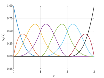
(a) Cubic $C^{1}$ B-splines

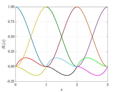
(b) Cubic Hermite splines

Figure 1: Cubic $C^{1}$ B-splines and cubic Hermite splines defined on an interval uniformly discretized in three elements. These two bases span the same function space.

When using nodal discretization scheme, the basis functions are the standard cubic Hermite splines. A discretization with $n_{e}$ elements leads to $6(n_{e}+1)$ dofs, i.e. the size of the vector $\Delta\bar{\boldsymbol{q}}$ consisting of unknown coefficients. We note that the cubic Hermite spline and the cubic $C^{1}$ B-splines span the same function space (see also Fig. 1).

4.3 Nodal discretization scheme with unit nodal director constraint

We now discuss the resulting matrix equations when enforcing the unit nodal director constraint (12) using different approaches. We focus here on the resulting equations for comparison purposes and refer to Appendix A for the derivation of associated matrices and further technical details.

4.3.1 Enforced constraint with Lagrange multipliers

Consider the semi-discrete formulation (3.2). Employing the implicit time integration scheme reviewed in Section 2.2 and linearizing the resulting nonlinear residual leads to the following matrix equations at the $k$-th iteration:

$$\underbrace{\begin{bmatrix}\bar{\mathbf{A}}+\mathbf{A}_{c}&\mathbf{J}^{T}_{n+\frac{1}{2}}\\ \mathbf{J}_{n+1}&\mathbf{0}\end{bmatrix}}_{\tilde{\mathbf{A}}}\,\begin{bmatrix}\Delta\bar{\boldsymbol{q}}_{n+1}^{k}\\ \Delta\boldsymbol{\lambda}_{n+\frac{1}{2}}^{k}\end{bmatrix}=\begin{bmatrix}\bar{\boldsymbol{F}}^{\text{ext}}_{n+\frac{1}{2}}-\bar{\boldsymbol{F}}-\mathbf{J}^{T}_{n+\frac{1}{2}}\boldsymbol{\lambda}_{n+\frac{1}{2}}\\ -\boldsymbol{\Psi}_{n+1}\end{bmatrix}\,,$$ (26)

where the matrix $\bar{\mathbf{A}}=\bar{\mathbf{A}}\left(\bar{\boldsymbol{q}}_{n+1}^{k-1},\bar{\boldsymbol{q}}_{n},\dot{\bar{\boldsymbol{q}}}_{n}\right)$ is the same as that in (25), $\mathbf{A}_{c}=\mathbf{A}_{c}\left(\boldsymbol{\lambda}_{n+\frac{1}{2}}^{k-1}\right)$ is the contribution of the unit nodal director constraint to the system matrix, i.e. the linearization of the term $\delta\bar{\boldsymbol{q}}\cdot\mathbf{J}^{T}(\bar{\boldsymbol{q}})\,\boldsymbol{\lambda}$ evaluated at $t_{n+\frac{1}{2}}$. For the derivation of $\mathbf{A}_{c}$, we refer to Appendix A.

We note that the two blocks of $\mathbf{J}^{T}$ and $\mathbf{J}$ of $\tilde{\mathbf{A}}$ are evaluated at two different time instances due to the holomonic type of the unit nodal director constraint, as discussed in ¹ Remark 2, p. 3834. Hence, $\tilde{\mathbf{A}}$ on the left-hand side of (26) is not a symmetric matrix, however, is a sparse matrix. (26) has the form of a saddle-point problem (SPP), for which we briefly recall the equivalence of the necessary and sufficient conditions for unique solution ⁷¹ p. 142:

• The matrix $\left(\bar{\mathbf{A}}+\mathbf{A}_{c}\right)$ is symmetric positive semi-definite, and

• The matrix $\mathbf{J}$ is full rank.

In general, these conditions are fulfilled for the studied rod formulation due to the definition of these matrices (see ² for $\bar{\mathbf{K}}$ and Appendix A for $\mathbf{A}_{c}$ and $\mathbf{J}$). We note that the number of degrees of freedom (dofs) is at most $(n_{e}+1)$ dofs more than that of (25), i.e. $7(n_{e}+1)$ dofs, due to at most $(n_{e}+1)$ additional unknown Lagrange multipliers. In cases of a clamped boundary condition or prescribed director, it requires a smaller number of unknown Lagrange multipliers. We note that here, we refer to the size of the vector $\left[\Delta\bar{\boldsymbol{q}}_{n+1}^{k}\;\Delta\boldsymbol{\lambda}_{n+\frac{1}{2}}^{k}\right]^{T}$ as the number of dofs, i.e. the number of unknown variables, for which we solve at each iteration.

4.3.2 Enforced constraint with Lagrange multiplier and nullspace methods

In this work, to eliminate the additional variable field of Lagrange multipliers in (3.2), i.e. to reduce the dimension of (26) to the same as that of (25), we employ the nullspace matrix $\mathbf{D}$ of the matrix $\mathbf{J}$, as discussed in the previous section. Consider the semi-discrete formulation (21), employing the implicit time integration scheme reviewed in Section 2.2 and linearizing the resulting nonlinear residual leads to the following matrix equations at the $k$-th iteration:

$$\underbrace{\begin{bmatrix}\mathbf{D}^{T}_{n+\frac{1}{2}}\bar{\mathbf{A}}+\mathbf{A}_{D}\\ \mathbf{J}_{n+1}\end{bmatrix}}_{\hat{\mathbf{A}}}\,\Delta\bar{\boldsymbol{q}}_{n+1}^{k}=\begin{bmatrix}\mathbf{D}^{T}_{n+\frac{1}{2}}\left(\bar{\boldsymbol{F}}^{\text{ext}}_{n+\frac{1}{2}}-\bar{\boldsymbol{F}}\right)\\ -\boldsymbol{\Psi}_{n+1}\end{bmatrix}\,,$$ (27)

where the counterpart $\mathbf{K}_{D}$ is the contribution of the nullspace matrix to the system matrix, i.e. the linearization of $\mathbf{D}^{T}_{n+\frac{1}{2}}$. For its derivation, we refer to Appendix A. We note that $\mathbf{D}^{T}_{n+\frac{1}{2}}$ depends on the nodal director from the previous iteration (see also Appendix A) and hence needs to be reassembled in each iteration and time step. Furthermore, the matrix multiplication by $\mathbf{D}^{T}_{n+\frac{1}{2}}$ is performed globally, also at each time step and iteration. The resulting matrix $\hat{\mathbf{K}}$ on the left-hand side of (27) is a sparse but not a symmetric matrix. The number of degrees of freedom is now the same as that of (25).

4.3.3 Enforced constrained with penalty method

An alternative approach is to weakly enforce the unit nodal director constraint (12) using the penalty method. Consider the semi-discrete formulation (3.2), employing the implicit time integration scheme reviewed in Section 2.2 and linearizing the resulting nonlinear residual leads to the following matrix equations at the $k$-th iteration:

$$\underbrace{\left(\bar{\mathbf{A}}+\mathbf{A}_{\beta,n+1}\right)}_{\check{\mathbf{A}}}\,\Delta\bar{\boldsymbol{q}}_{n+1}^{k}=\bar{\boldsymbol{F}}^{\text{ext}}_{n+\frac{1}{2}}-\bar{\boldsymbol{F}}-\beta\,\mathbf{J}^{T}_{n+1}\boldsymbol{\Psi}_{n+1}\,,$$ (28)

where $\mathbf{A}_{\beta,n+1}$ is the contribution of the penalty term to the system matrix, i.e. the linearization of the penalty term $\left(\beta\,\delta\bar{\boldsymbol{q}}\cdot\mathbf{J}^{T}(\bar{\boldsymbol{q}})\,\boldsymbol{\Psi}\right)$ evaluated at the time instance $t_{n+1}$. For its derivation, we refer to Appendix A. We note that the resulting matrix $\check{\mathbf{A}}$ on the left-hand side of (28) is a sparse and symmetric matrix. The number of degrees of freedom is the same as that of (25).

5 Computational cost

In this section, we discuss the computation cost corresponding to the five formulations discussed in the previous two sections, listed in Table 1. Particularly, we compare the sparsity, bandwidth, and symmetry of the system matrix. We also discuss the number of degrees of freedom (dofs) of each formulation. In Table 2, we give an overview of these properties for the five studied formulations. For the notation simplicity, we refer to the studied formulations using the abbreviations given in italics in Table 2.

Discretization scheme		Matrix equations	System matrix	Number of dofs1
Isogeometric discretizations (IGA)		Equation2 (23), (24)⋆	sparse, symmetric	$3[ne(p-r)+r+1]$
Nodal discretization scheme without unit nodal director		Equation (25)	sparse, symmetric	$6(n_{e}+1)$
constraint (Nodal $\mathbb{R}^{3}$)
Nodal discretization	strong enforcement using Lagrange	Equation (26)	sparse, non-	$7(n_{e}+1)$
scheme with unit	multiplier method (Nodal SPP)		symmetric
nodal director con-	strong enforcement with reduced	Equation (27)⋆⋆	sparse, non-	$6(n_{e}+1)$
straint	equations using Lagrange multi-		symmetric
	plier and nullspace methods
	(Nodal SPP-reduced)
	weak enforcement using penalty	Equation (28)	sparse, symmetric	$6(n_{e}+1)$
	method (Nodal-penalty)
⋆: Global matrix multiplication is required. The multiplier is a constant matrix.
⋆⋆: Global matrix multiplication is required. The multiplier is reassembled at each iteration and time step.
1 i.e. the size of the unknown increment vector on the left-hand side, for which we solve at each iteration.
2 Using the strong approach of outlier removal 70 leads to a smaller number of dofs than $3[ne(p-r)+r+1]$, depending on
the type of Dirichlet boundary conditions.

Table 2: Different matrix equations for the studied semi-discrete formulations listed in Table 1, using either isogeometric or nodal discretizations.

Focusing on the number of degrees of freedom (dofs) when using the nodal discretization scheme, we see that strongly enforcing the unit nodal director constraint using the Lagrange multiplier method (Nodal SPP) leads to the highest number of dofs due to the additional unknown Lagrange multipliers. This can be reduced to the same number of dofs $6(n_{e}+1)$ by eliminating the Lagrange multipliers using the nullspace method (Nodal SPP-reduced), or weakly enforcing the same constraint using the penalty method (Nodal-penalty), or neglecting the unit nodal director constraint (Nodal $\mathbb{R}^{3}$) (see Table 2). Focusing on the number of degrees of freedom (dofs) when using isogeometric discretizations, employing quadratic $C^{1}$ splines leads to $3(n_{e}+2)$ dofs, less than $6(n_{e}+1)$ when using nodal discretizations with the same number of elements. Using cubic $C^{1}$ splines that span the same function space as the cubic Hermite splines employed for the nodal scheme, leads to $6(n_{e}+1)$ dofs, the same as the smallest number of dofs when using the nodal scheme. Using cubic $C^{2}$ splines leads to either the same dofs of $6(n_{e}+1)$ when using one element, i.e. $n_{e}=1$, or less than $6(n_{e}+1)$ with $n_{e}>1$. Using splines of higher polynomial degrees $p$ and higher order of continuity $r$ may lead to more than $6(n_{e}+1)$ dofs, except the cases with a very large number of elements. In summary, the isogeometric discretization scheme enables quadratic basis functions that are one order lower than Hermite splines and a smaller number of dofs than using the nodal scheme, particularly when using a significantly large number of elements. We note that for the studied rod formulation, a significantly large number of elements is generally not required and thus the number of dofs is not decisive for the difference in the computational cost when using isogeometric or nodal discretizations.

Figure 2: Band structure of the system matrix using isogeometric and nodal discretization schemes with different approaches.

Focusing on the sparsity of the system matrix, we see that we obtain a sparse matrix in all cases. Moreover, as discussed above, a significantly large number of elements and thus also the number of dofs is generally not required, using either isogeometric or nodal discretizations requires similar memory storage for the system matrix. Another essential factor that affects the computational cost per iteration is the symmetry of the system matrix since solving a symmetric system generally requires less effort than solving a non-symmetric one when using a standard solver. As discussed in the previous section and summarized in Table 2, we observe that using the nodal discretization scheme with strong enforcement of the unit nodal director constraint leads to a non-symmetric matrix while all the other three approaches lead to a symmetric matrix. We note that Table 2 and this observation holds for Equations (23)-(28) which correspond to dynamics computations. In static cases, the strong enforcement using Lagrange multiplier method (Nodal SPP), however, leads to a symmetric system matrix, while the system matrix resulting from the strong enforcement with reduced equations using both Lagrange multiplier and nullspace methods (Nodal SPP-reduced) remains non-symmetric.

In Figure 2, we illustrate the band structure of the system matrix on the left-hand side of the matrix Equations (23)-(28) for the five studied formulations. For this illustration, we consider an exemplary fixed-fixed cable commonly employed for airborne wind turbines, which is a cable DuPont’s Kevlar 49 type 968. This type of cable has elastic constants of $E_{11}=81.8$ GPa, a mass density of $\rho=1.429\cdot 10^{3}$ kg/m³, an initial length of $L_{0}=300$ m, and a cross-sectional diameter of $0.007$ m. We discretize the cable with 20 elements in all cases and compute the matrices at the first time step and the second iteration to include the contribution of all terms. Since we want to focus on the symmetry and band structure of the system matrix, we employ cubic $C^{1}$ splines when using IGA to obtain the same number of dofs. For illustration purposes, we have removed the constrained degrees of freedom due to the fixed boundaries in all cases. Focusing on IGA (Figures 2a and b), we observe that the employed outlier removal approach ⁷⁰ does not change the band structure or the symmetry of the system matrix, but only reduces its dimension since constraints are directly built into the spline space, as discussed in ^{2, 70}. Focusing on the nodal scheme with strong enforcement of the unit nodal director constraint (Figures 2c and d), we see the larger system matrix when using Nodal SPP and a non-symmetric matrix when using Nodal SPP-reduced. The matrix obtained with Nodal SPP appears symmetric, however, is a non-symmetric matrix in dynamics computations since the top-right and bottom-left block matrices are evaluated at different time instances, as discussed in the previous section. Using the penalty method to weakly enforce the unit nodal director constraint or neglecting it (Figures 2e and f, respectively) leads again to a symmetric matrix. Furthermore, we can see in Figure 2 that using the isogeometric or nodal discretizations without strong enforcement of the unit nodal director constraint leads to a similar bandwidth of the system matrix. As discussed in ², this occurs regardless of the fact that spline basis functions employed for IGA have larger supports up to $p+1$ elements than that of nodal discretizations (see also ⁴³ p. 92-97). Notably, employing basis functions with larger support does not always lead to more evaluation per quadrature point. Using IGA, there are up to $p+1$ basis functions that have support in an element (see also Figure 1). For the studied rod formulation, using splines of $p<4$ leads to either less (if $p=2$) or the same (if $p=3$) number of active basis functions per element as using the nodal scheme.

In Table 2, we also highlight that using IGA with the strong outlier removal approach ⁷⁰ or Nodal SPP-reduced requires global matrix multiplication (see also Equations (24) and (27)). This increases the computational cost, particularly for significantly large systems. On the one hand, using IGA with the strong outlier removal approach involves a constant multiplier, the extraction operator $\mathbf{C}$, which does not require any reassembly or update per iteration. Using Nodal SPP-reduced, on the other hand, we need to reassemble the nullspace matrix $\mathbf{D}$ at each iteration since $\mathbf{D}$ depends on the nodal directors of the current configuration (see also Appendix A). Moreover, we note that compared to IGA and Nodal $\mathbb{R}^{3}$, i.e. the nodal discretization scheme without considering unit nodal director constraint, the enforcement of this constraint requires the evaluation of additional terms, such as the constraint or the penalty terms, and hence requires the assembly of additional matrices and vectors on the left- and right-hand sides of the matrix equations.

6 Numerical examples

In this section, we investigate the accuracy and computational cost of the studied semi-discrete rod formulations discussed in the previous sections (see also Tables 1 and 2). To gain more insights, we first numerically study the condition number of the system matrix which depends on different parameters such as the penalty factor, the employed outlier removal approach, and the length of the nodal directors. We then numerically illustrate via an example of a planar roll-up that preserving nodal directors in the unit sphere leads to better accuracy than nodal directors in $\mathbb{R}^{3}$. Via a static and dynamic analysis of exemplary cables, we show that cubic $C^{1}$ isogeometric discretization leads to the same responses in the static case, however, slightly larger responses in parts of the dynamic computation. We also illustrate that IGA with or without outlier removal averagely requires a smaller computational time per iteration than using any formulations based on the nodal scheme. For fine meshes, using Nodal SPP-reduced requires the most time per iteration compared to other approaches. We also numerically demonstrate via these examples that using the nodal scheme with strongly enforced unit nodal director constraint leads to zero nodal axial stress resultants, as discussed in the previous sections.

6.1 Numerical study of the condition number of the system matrix

The condition number of the system matrix in the matrix equations plays an essential role in ensuring the convergence of the Newton-Raphson iterative procedure, which is associated with the robustness of the corresponding formulation. Hence, to gain better insights into the influence of different parameters such as the penalty factor, the outlier removal approach, and the length of the nodal directors on this number, as well as insights into the robustness of each formulation for the same number of elements, we numerically study and compare this obtained with five semi-discrete formulations considered in this work (see also Tables 1 and 2). We consider an exemplary cable commonly employed for airborne wind turbines, which is a cable DuPont’s Kevlar 49 type 968. This type of cable has elastic constants of $E_{11}=81.8$ GPa, a mass density of $\rho=1.429\cdot 10^{3}$ kg/m³, an initial length of $L_{0}=300$ m, and a cross-sectional diameter of $0.007$ m. The cable is fixed on both ends and subjected to its self-weight. We discretize the cable with 40 elements using five formulations discussed in the previous sections. Since we focus on the condition number, we choose cubic $C^{1}$ splines for the isogeometric discretization to obtain the same number of dofs as the nodal scheme. We compute the condition number of the system matrix at the first load step and the first iteration for all formulations.

Figure 3: Condition number of the system matrix as a function of the penalty factor $\beta$.

Figure 4: Condition number of the system matrix as a function of the enforced length for the nodal directors.

We first investigate the effect of the penalty factor on the condition number of the system matrix when using Nodal-penalty. In Figure 3, we plot this number as a function of the penalty factor $\beta$ in a logarithmic scale. We compare the condition number obtained with Nodal-penalty (purple curve), Nodal $\mathbb{R}^{3}$ (green line), and IGA with (blue dashed line) and without (blue continuous line). We consider the system matrix employed for both static (Figure 3a) and dynamic cases (Figure 3b). Focusing on the purple curve, we observe that increasing the penalty factor $\beta$ increases the condition number in both cases. This necessarily means that a significantly large penalty factor can lead to ill-conditioning of the system matrix, reducing the robustness of the corresponding formulation Nodal-penalty. For the studied cable, the penalty terms start having an effect on the condition number of the system matrix when the penalty factor is larger than $10^{4}$ (see also inset figures in Figure 3). Using smaller penalty factors leads to approximately the same condition number as using Nodal $\mathbb{R}^{3}$ , as expected. Focusing on the green and blue lines, we see that using IGA generally leads to a smaller condition number than Nodal $\mathbb{R}^{3}$. In the static case, employing the strong approach of outlier removal ⁷⁰ slightly increases this to approximately the same condition number as using Nodal $\mathbb{R}^{3}$. In the dynamic case, however, the outlier removal approach reduces the condition number by several orders of magnitude. This is consistent with the observations and discussions in ² that using the outlier removal approach ⁷⁰ improves the robustness of isogeometric discretizations for dynamics computations. Based on this observation, in this work, we generally employ the outlier removal approach only for dynamic computations, unless it is stated otherwise. Furthermore, comparing the condition number obtained in the static and dynamic cases, we can see that the obtained condition number in the dynamic case is several orders of magnitude smaller than that in the static case. This necessarily means that the terms regarding the mass matrix improve the conditioning of the system matrix, improving the robustness of the studied formulations. We conclude that the penalty factor should be chosen as large as required to enforce the unit nodal director constraint such that it does not negatively affect the condition number of the resulting system matrix. For dynamics computations, the outlier removal approach ⁷⁰ improves the conditioning of the system matrix, leading to better robustness when using IGA, as discussed in ².

A well-established approach to improve the conditioning of the system matrix for thin-walled structures is the scaled director conditioning ^{57, 72, 73}. The idea is to scale the length of the director variable field to reduce the condition number of the resulting system matrix. Hence, we also investigate whether this approach improves the conditioning for the studied semi-discrete formulations when using the nodal discretization scheme. We employ this approach by replacing the constrained nodal directors $\boldsymbol{d}_{h}$ in the discretization (11) by $\frac{1}{\alpha_{d}}\hat{\boldsymbol{d}}_{h}$ and enforcing a length of $\alpha_{d}$ for $\hat{\boldsymbol{d}}_{h}$. We note that the resulting nodal directors are then still constrained to have a unit length. In Figure 4, we plot the condition number of the system matrix as a function of the scaling factor $\alpha_{d}$ when using Nodal-penalty (purple curve), Nodal SPP (orange curve), and Nodal SPP-reduced (dark red curve). When using Nodal-penalty, to avoid the effect of the penalty factor on the condition number, we choose a small penalty factor of $\beta=1.0$. For comparison purposes, we also include the condition number obtained when using Nodal $\mathbb{R}^{3}$ (green line) and IGA without outlier removal (blue line). The inset figures focus on the region close to the minimum of the condition number with respect to $\alpha_{d}$.

Focusing on the purple curve obtained with Nodal-penalty, we observe that we obtain a minimal value with $\alpha_{d}=10$. Increasing $\alpha_{d}$ increases the condition number that is then several orders of magnitude larger than that obtained with Nodal SPP or Nodal SPP-reduced using the same value of $\alpha_{d}>10$. Focusing on the dark red curve obtained with Nodal SPP-reduced, we see that we obtain a minimal value without scaling the enforced length, i.e. $\alpha_{d}=1.0$. Compared to the minimum obtained with Nodal-penalty or Nodal SPP, the obtained value is the smallest minimum that is slightly smaller than the condition number obtained with IGA in the static case and is the same as that in the dynamic case. Comparing the dark red and orange curves, we also see that reducing the system of equations using the nullspace method significantly improves the conditioning of the system matrix. Focusing on the orange curve obtained with Nodal SPP, we observe that we obtain a minimal condition number with $\alpha_{d}=10$ and $\alpha_{d}=100$ in the static and dynamic cases, respectively. The obtained minimal value is the same as the minimum when using Nodal-penalty in the static case and is one order of magnitude larger in the dynamic case. We conclude that when strongly enforcing the unit nodal director constraint, reducing the system of equations using nullspace method (Nodal SPP-reduced) also improves the conditioning of the system matrix and hence the robustness of the corresponding formulation. One does not need to employ the scaled director conditioning approach to further reduce the condition number. Using Nodal SPP-reduced can lead to a similar condition number as using IGA. When strongly enforcing the unit nodal director constraint using Nodal SPP or weakly enforcing this using Nodal-penalty, the scaled director conditioning approach can improve the conditioning, however, requires a parameter study in advance to estimate optimal scaling factors.

6.2 Convergence study of a planar roll-up

Figure 5: Deformed configurations of the clamped rod bent to a circle at different load steps, computed with cubic $C^{1}$ isogeometric discretization without outlier removal approach and a mesh of 8 elements.

Figure 6: Axial stress and bending moment resultants in the final configuration of a planar roll-up, computed with cubic isogeometric and nodal discretizations.

Figure 7: Convergence of relative errors of the clamped rod bent to a circle computed with cubic isogeometric and nodal discretizations.

We now investigate the accuracy and convergence achieved with the studied semi-discrete formulations. To this end, we consider a planar roll-up example of pure bending with a well-known final configuration and stress resultants. Since we focus on the accuracy achieved with different spatial discretization schemes, we employ cubic $C^{1}$ splines when using IGA throughout this subsection, which belong to the same space as the Hermit splines employed for nodal discretization schemes. We consider a rod with an initital length of $L=40$ m, axial stiffness of $EA=100$ N, and bending stiffness of $EI=200$ Nm², which we discretize with 40 elements in all cases. The rod is clamped at the left-end and subjected to a bending moment $M=2\pi EI/L$ that is to roll the rod to one full circle and is applied in 55 load steps, illustrated in Figure 5. We strongly enforce the Dirichlet boundary conditions in the standard way and employ a tolerance of $10^{-10}$ for the convergence of the Newton-Raphson method in all cases. Figure 5 also shows five snapshots of the deformed configurations, computed with the cubic $C^{1}$ isogeometric discretization. We obtained the same configurations when using Nodal-penalty, Nodal SPP, or Nodal SPP-reduced, and hence discarded these in Figure 5 purely for the sake of illustration clarity. For this example, using Nodal $\mathbb{R}^{3}$ leads to an ill-conditioned system matrix and thus the Newton-Raphson scheme does not converge. When using Nodal-penalty, based on empirical results, we observed that using small penalty factors $\beta\leq 10^{2}$ leads to an ill-conditioned system matrix, while using $\beta\leq 10^{6}$ requires more than 10 iterations per load step. Hence, we choose a penalty factor of $\beta=10^{6}$ for our computations, which requires a maximum of 8 iterations per load step. Using IGA, Nodal SPP, or Nodal SPP-reduced requires a maximum of 6 iterations per load step.

Figure 6 illustrates the axial stress resultants (Figures 6a and b) and the bending moment resultants (Figures 6c and d) in the circular configuration at the last load step, obtained with IGA and Nodal SPP. Using Nodal SPP-reduced or Nodal-penalty with $\beta=10^{6}$ leads to the same stress resultants as Nodal SPP. Hence, we compare the results obtained with IGA and Nodal SPP in Figure 6. We also include the reference value (black curves) of the stress resultants for this pure bending example. Focusing on the bending moment resultants in Figures 6c and d, we observe that both discretization schemes lead to stress resultants consisting of oscillations around the reference value along the rod. Focusing on the axial stress resultants in Figures 6a and b, we see that both schemes also lead to oscillating responses. When using Nodal SPP, this oscillation in the axial stress resultants is caused by zero nodal values since the nodal directors are constrained to a unit length, as discussed in Section 3.1. Nevertheless, the axial stress resultants oscillate around a non-zero value, when using either Nodal SPP or IGA. We note that based on empirical results, increasing the polynomial degree or continuity order when using IGA, or refining the mesh when using either one of the four aforementioned formulations reduces the magnitude of the oscillations in the stress resultants. These results imply the typical effect of membrane locking on stress resultants ³⁴. We note that for geometrically nonlinear problems, another locking phenomenon has been reported for shell structures in ⁷⁴. This requires further study in future work to identify whether this occurs for the studied rod formulation.

Figure 7 illustrates the convergence of the relative errors in $L^{2}$-, $H^{1}$-, and $H^{2}$-norms of the studied planar roll-up, obtained with isogeometric and nodal discretizations. We again obtain the same accuracy and convergence behavior in all three error norms when using Nodal-penalty, Nodal SPP, and Nodal SPP-reduced. Hence, we plot the results obtained with Nodal SPP (orange curves with circle markers) and compare with those obtained with IGA based on cubic $C^{1}$ (blue curves with cross markers) and $C^{2}$ (blue curves with triangle markers) splines. Focusing on the blue curves, we observe that increasing the continuity order of cubic spline functions increases the accuracy in all cases, as discussed also in ². Focusing on the convergence in the $L^{2}$- and $H^{1}$-norms (Figures 7a and b), we see that using IGA with either cubic $C^{1}$ or $C^{2}$ splines, on the one hand, leads to a similar convergence rate as Nodal SPP, on the other hand, leads to higher error level. For the errors in $H^{2}$-norm (Figure 7c), we have the same observations when using IGA with cubic $C^{1}$ splines. Using cubic $C^{2}$ splines leads to approximately the same error level and a slightly higher convergence rate. We conclude that using the nodal discretization scheme that preserves the nodal director field in the unit sphere leads to better accuracy in the deformations in different error norms than using IGA. The nodal scheme without this property, i.e. Nodal $\mathbb{R}^{3}$ or Nodal-penalty with small penalty factors, may lead to an ill-conditioned system matrix and hence is generally less robust than IGA, Nodal SPP, and Nodal SPP-reduced. Furthermore, we also study the convergence of the considered planar roll-up with different slenderness ratios in Appendix B. We observe the typical pre-asymptotic plateau in the convergence curves for large slenderness ratios, which becomes more severe with increasing slenderness ratios in all cases. This implies the effect of membrane locking on the accuracy of the spatial discretization schemes, which is consistent with the observations in the stress resultants discussed above. In this work, we focus on the comparison between different semi-discrete rod formulations and hence plan to investigate this locking effect and locking-preventing techniques for the studied rod formulation in future work.

6.3 Static analysis of a catenary

Figure 8: Final deformed configuration of an exemplary cable subjected to its weights and a linear wind profile with a prescribed fairlead position, computed with cubic $C^{1}$ isogeometric discretization without outlier removal.

Figure 9: Axial stress resultants in the final configuration of the cable in Figure 8, computed with isogeometric and nodal discretization schemes.

Figure 10: Bending moment resultants in the final configuration of the cable in Figure 8, computed with isogeometric and nodal discretization schemes.

Number of elements	IGA1	Nodal $\mathbb{R}^{3}$	Nodal SPP	Nodal SPP-reduced	Nodal-penalty2
$2^{3}$	21	21	12	24	20
$2^{4}$	13	13	13	13	13
$2^{5}$	21	21	17	15	13
$2^{6}$	18	$-$3	18	18	20
$2^{7}$	17	17	26	22	31
$2^{8}$	23	23	39	25	21
1 The maximum number of iterations is the same for both cases with and without outlier removal.
2 $\beta=10^{6}$.
3 The system matrix is ill-conditioned. The Newton-Raphson scheme did not converge.

Table 3: Maximum number of iterations for the Newton-Raphson scheme when using different discretization schemes. This occurred once at the 52^nd load step, when we start moving the right-end of the cable in Figure 8 to the final fairlead position.

Figure 11: Computation time per iteration, averaged over all iterations and load steps, required when using isogeometric and nodal discretization schemes for the cable in Figure 8.

We now investigate the performance of the considered semi-discrete rod formulations, in terms of the obtained responses and computational time, for examples that are relevant and common for studying mooring lines in offshore wind engineering. The first example is a static analysis of an exemplary cable of the DuPont’s Kevlar 49 type 968, which is also considered in Section 6.1. The cable lies initially straight along the $X$-axis and is fixed at its left-end while we move the right-end from the initial position of $(L_{0},0,0)$ to a prescribed fairlead position of $(50,0,280)$. We consider the self-weight of the cable and the following linear wind profile along the $Z$-axis (see also Figure 8):

$$v_{\text{wind}}(z)=15\,\frac{z}{100}\;[\text{m/s}]\,.$$ (29)

To activate the inertial stiffness of the cable, we first prestress the cable by moving the right-end to $(L_{0}+0.01,0,0)$ in one load step. We then apply the self-weight in 50 load steps while keeping the right-end at the prestressed position. After the self-weight is fully applied, we move the right-end to the prescribed fairlead position in 400 load steps. We compute the response of this cable using the five semi-discrete formulations: IGA, Nodal $\mathbb{R}^{3}$, Nodal-penalty, Nodal SPP, and Nodal SPP-reduced. We discretize the cable in 40 elements and employ a tolerance of $10^{-10}$ for the convergence of the Newton-Raphson method in all cases. We again focus on the performance of different discretization schemes and hence employ basis functions in the same function space, i.e. cubic $C^{1}$ and Hermite splines. When using nodal discretizations, we enforce the homogeneous boundary condition at the left-end in the standard way but using the extraction operator to enforce this when using IGA for the sake of implementation when employing the outlier removal approach ⁷⁰. Nevertheless, the prescribed right-end is enforced at each step in the standard way for all formulations. The maximum number of iterations for all formulations is 18 when we start moving the right-end to the fairlead position, i.e. at the 52^nd load step. For all remaining load steps, all formulations require a maximum of 6 iterations.

Figure 8 illustrates the final configuration of the studied cable obtained with cubic $C^{1}$ isogeometric discretization without outlier removal. Using either Nodal $\mathbb{R}^{3}$, Nodal-penalty, Nodal SPP, Nodal SPP-reduced, or IGA with outlier removal leads to the same configuration. Hence, for illustration clarity, we plot only one result in Figure 8. In Figure 9, we plot the axial stress resultants obtained with each formulation. When using IGA, the outlier removal approach does not affect the accuracy (see also ^{2, 70}), we refer to IGA for both cases with and without outlier removal in the following. Focusing on the blue and green curves obtained with IGA and Nodal $\mathbb{R}^{3}$, respectively, in Figure 8a, we observe that these two schemes lead to the same result. This is expected since we employ basis functions in the same function space for these schemes. We note that the axial stress resultants obtained with these two formulations consist of slight oscillations, which may be due to membrane locking, as discussed in the previous example of a planar roll-up. We also see that using Nodal-penalty with a penalty factor of $\beta=10^{3}$ (purple curve in Figure 8a), the unit nodal director constraint is not enforced effectively, leading approximately to the same axial stress resultants as using IGA or Nodal $\mathbb{R}^{3}$. Increasing $\beta$ enforces this constraint more effectively, however, leading to constrained nodal axial stress values and thus to oscillations in the axial stress resultants, as illustrated in Figure 8b for a larger value of $\beta=10^{6}$. We note that for this example, a penalty factor of $\beta=10^{6}$ is not enough to enforce the unit nodal director constraint and hence the nodal axial stresses are not zero. Strongly enforcing this constraint using either Nodal SPP or Nodal SPP-reduced leads to axial stress resultants with zero nodal values, i.e. oscillating resultants, as discussed in Section 3.1. We also see that reducing the system of equations of Nodal SPP using the nullspace method does not affect the accuracy and thus leads to the same results. Figure 10 illustrates the bending moment resultants obtained with the five aforementioned formulations. We observe that all formulations lead to approximately the same result. We see a slight difference in nodal values due to the enforced unit nodal director constraint, either weakly or strongly.

In terms of computational cost, we investigate the maximal number of iterations and computing time per iteration when using the studied formulations under mesh refinement. In Table 3, we list the maximum number of iterations required for the 52^nd load step. Focusing on the first two columns, we observe that using IGA and Nodal $\mathbb{R}^{3}$ requires the same number of iterations. Using Nodal $\mathbb{R}^{3}$, however, can lead to an ill-conditioned system matrix, e.g. for the mesh of $2^{6}$ elements for the studied cable. Compared with these two formulations, using Nodal SPP requires fewer iterations for coarser meshes and, nonetheless, more iterations for finer meshes. We also see that using Nodal SPP-reduced and Nodal-penalty requires approximately the same number of iterations as IGA or Nodal $\mathbb{R}^{3}$. In Figure 11, we plot the averaged computing time per iteration and load step when using the aforementioned formulations. We observe that using IGA (blue curves) requires slightly less time for computing per iteration than using any of the nodal schemes. We see that using outlier removal (blue dashed curve) requires approximately the same time as without outlier removal (blue solid curve). This is expected since we employ the extraction operator to enforce the homogeneous boundary condition, i.e. we perform a global matrix multiplication in each iteration in both cases. We note that although we enforce the boundary condition in a more expensive way when using IGA than the standard way when using the nodal scheme, IGA requires less time per iteration than the nodal scheme. This necessarily means that for this example, the global multiplication is not decisive for the computational cost per iteration. Focusing on the green, orange, and purple curves, we observe that using Nodal $\mathbb{R}^{3}$, Nodal SPP, and Nodal-penalty requires the same computing time per iteration. Using Nodal SPP-reduced requires approximately the same time on coarser meshes, however, significantly more computational effort on finer meshes. This is due to the reassembly of the nullspace matrix $\mathbf{D}$ at each iteration, as discussed in Section 5.

We conclude that for the static analysis of the studied cable, the cubic isogeometric and nodal discretizations show approximately the same accuracy in the deformed configuration and bending moment resultants. A nodal scheme with strongly enforced unit nodal director constraint leads to zero nodal axial stresses and hence oscillating axial stress resultants. A nodal scheme without this constraint leads to the same axial stress as the isogeometric scheme. In general, all studied semi-discrete formulations require a similar number of iterations for this example. However, Nodal $\mathbb{R}^{3}$ seems to be the least robust formulation compared to others since it can lead to an ill-conditioned system matrix. Per iteration, IGA requires the smallest computing time despite the global matrix multiplication with the constant extraction operator. Nodal $\mathbb{R}^{3}$, Nodal-penalty, and Nodal SPP require approximately the same computing time despite the evaluation of additional penalty terms and a larger system of equations of the saddle-point problem. Nodal SPP-reduced requires approximately the same computing time as these three formulations on coarser meshes, however, significantly more computational effort on finer meshes.

Figure 12: Snapshots of a mooring line subjected to a logarithmic current speed profile in open water, computed with cubic $C^{1}$ isogeometric discretization and the outlier removal approach ⁷⁰. The snapshots in the last 10 seconds and the final configuration from ⁷⁵ Ch. 7.6.4, p. 257 (black solid curve) are not distinguishable in this axis scale. The horizontal black dashed line represents the numerical barrier.

Figure 13: Axial stress and bending moment resultants in the final configuration (at $t=T$) of the mooring line in Figure 12, computed with isogeometric and nodal discretization schemes.

Figure 14: Time history of the displacement and velocity of the fairlead of the mooring line in Figure 12, computed with isogeometric and nodal discretization schemes.

Figure 15: Time history of the energy of the mooring line in Figure 12, computed with isogeometric and nodal discretization schemes.

Figure 16: Computation time per iteration, averaged over all iterations and load steps, required when using isogeometric and nodal discretization schemes for the mooring line in Figure 12.

6.4 A dynamics example of mooring lines

The second example of mooring lines considered in this work is a cable commonly employed in offshore wind engineering adapted from ⁷⁵ Ch. 7.6.4, p. 257. The cable has an initial length of $L_{0}=627$ m, a weight per unit length when submerged in water of $w_{s}=2.46$ kN/m, a Young modulus of $E=5.6\cdot 10^{10}$ N/m², and a cross-sectional area of $A=0.0159$ m². The cable’s left-end is fixed on the seabed while its right-end is also moved to a fairlead position with a prescribed point load in this case. This point load and the final configuration of the cable are provided by the author of ⁷⁵. We note that F.G. Nielsen computed the final configuration by finding cable parts that rest on the seabed and deform due to the point load and cable’s self-weights when submerged in water, considering the cable a sort of an elastic catenary and neglecting the effects of the water current. The provided solution is not based on a dynamic analysis but on a static one. In our computations, we want to capture and investigate the responses when the right-end is moved and the possible effects of the water current. Hence, we simulate the moving procedure as a dynamic analysis of the studied cable and consider the following logarithmic current speed profile (see also Figure 12):

$$v_{\text{wind}}(z)=2\,\log\left(1+\frac{9}{z_{\text{seabed}}}\,z\right)\;[\text{m/s}]\,,$$ (30)

which can be employed for open water (see e.g. ⁷⁶). We simulate the seabed at $z_{\text{seabed}}=100$ m as a numerical barrier using the so-called barrier function ^{77, 78, 79}. The main idea is to add a penalty term of the barrier function to the weak form (7), which introduces increasing energy/work when the distance between the rod and the barrier decreases and vice versa, i.e. the energy required to keep a distance between all point of the current configuration and the barrier. We note that this necessarily means that there is a numerical gap between the discrete rod configuration and the barrier, which can be regulated with the penalty factor associated with the barrier term. For more details on the barrier function and the linearization of associated terms for the studied rod formulation, we refer to ⁷⁹. For our computation, we consider a numerical barrier at $z=-0.5$ m such that a part of final configuration rests at a height of $z=0$. We choose a reciprocal function as the barrier function and an associated penalty factor of 25. We enforce the cable’s weight and the prescribed point load at the right-end in 10 seconds with a time step of $0.01$ s. We continue the simulation with the constant final values of these forces in 20 seconds with the same time step, such that a part of the cable deforms and rests “on” the numerical barrier and reaches the final configuration. Similar to the static analysis above, we compute the response of this cable using the five semi-discrete formulations: IGA, Nodal $\mathbb{R}^{3}$, Nodal-penalty, Nodal SPP, and Nodal SPP-reduced. We discretize the cable in 40 elements and employ a tolerance of $10^{-10}$ for the convergence of the Newton-Raphson method in all cases. We again focus on the performance of different discretization schemes and hence employ basis functions in the same function space, i.e. cubic $C^{1}$ and Hermite splines. We enforce the homogeneous boundary condition on the left boundary in the same way as described in the static analysis above. The number of iterations is 4 for all studied formulations at each time step.

Figure 12 illustrates six snapshots every 5 seconds of the simulation, computed with cubic $C^{1}$ isogeometric discretization and outlier removal. We also include the provided final configuration of ⁷⁵ Ch. 7.6.4, p. 257 (black solid curve) and the numerical barrier (black dashed horizontal line). Also for this example, we obtain indistinguishable configurations when using IGA without outlier removal or the other four formulations based on the nodal discretization scheme. Hence, we also plot the results of one formulation here purely for illustration clarity. Since we obtain the same responses when using IGA with and without outlier removal, we refer to IGA for both of these cases in the following. Comparing the configuration during the last 10 seconds with the provided solution of ⁷⁵ Ch. 7.6.4, p. 257, we see that they approximately overlap each other. This necessarily means that the effect of the considered current speed on the final configuration is negligible. Figure 13 illustrates the axial stress and bending moment resultants in the final configuration of the studied cable, computed with the aforementioned formulations. Focusing on axial stress resultants (Figure 13a), we observe that using IGA (blue curve) or Nodal $\mathbb{R}^{3}$ (green curve) leads to similar axial stresses. We see that using Nodal-penalty (purple curve) with a penalty factor of $\beta=10^{6}$ does not effectively enforce the unit nodal director constraint and thus leads to the same axial stress resultants as Nodal $\mathbb{R}^{3}$. Strongly enforcing this constraint using either Nodal SPP (orange curve) or Nodal SPP-reduced (dark red curve), however, leads to zero nodal axial stresses, as observed and discussed in previous sections and examples. We note that also for this example, reducing the system of equations of Nodal SPP using Nodal SPP-reduced leads to the same stress resultants. Focusing on the bending moment (Figure 13b), we observe that using IGA leads to results consisting of oscillations with larger amplitude than that obtained with the other four formulations based on the nodal scheme. This is caused by the lower accuracy in deformations in different error norms achieved with the chosen cubic $C^{1}$ splines and mesh size for this example and can be improved by refining the mesh and/or the continuity order (see also the convergence study in Section 6.2). We note that using any of the four formulations based on the nodal discretization scheme leads to bending moments that also oscillate but with significantly smaller amplitude. The nodal values obtained with these formulations differ from each other due to the enforced unit nodal director constraint.

Figure 14 illustrates the time history of the displacement and velocity at the right-end of the cable, i.e. the fairlead. We observe that all four formulations based on the nodal scheme lead to the same responses. Using IGA leads to slightly larger displacements between $t=10$ and $t\approx 28$ seconds and oscillating velocity with larger amplitude. We see that at $t=30$ seconds, i.e. towards the end of the simulation, we obtain again approximately the same responses. This necessarily means that for this example, using IGA requires longer computation to reach the same final responses. We note that the reason for this observed difference might be the remaining outliers and/or activated high-frequency modes when using IGA (see also ²). In Figure 15, we plot the time history of the potential, kinetic, and total energy obtained with the studied formulations. We observe that using the formulations based on the nodal scheme leads to approximately the same energy responses. We also see a slight difference in these responses when strongly enforcing the unit nodal director constraint. This is expected since this constraint leads to different nodal stress resultants. Focusing on the blue curves obtained with IGA, we observe that it leads to slightly larger energy than using the nodal scheme, which is due to slightly larger responses observed in Figure 14. Towards the end of the computation, we again obtain approximately the same energy responses as using the nodal discretization scheme.

In terms of computational cost, we also investigate the number of iterations and computing time per iteration when using the studied formulations under mesh refinement. For this dynamic example, all formulations require the same number of iterations per time step that is 4 iterations per time step. In Figure 16, we plot the averaged computing time per iteration and time step when using the studied formulations. We have the same observations as in the static analysis above: IGA (blue curves) requires the least computing time per iteration despite the global matrix multiplication for enforcing the boundary conditions and employing the outlier removal approach ⁷⁰. Using Nodal $\mathbb{R}^{3}$, Nodal SPP, Nodal-penalty, and Nodal SPP-reduced requires the same computing time per iteration. One exception is Nodal SPP-reduced for computations on fine meshes, which requires significantly more computational effort due to the reassembly of the nullspace matrix per iteration.

We conclude that for the dynamic analysis of the exemplary mooring line, all four formulations based on the nodal discretization scheme lead to approximately the same responses, except the axial stress resultants which are constrained to zero nodal value when strongly enforcing the unit nodal director constraint. For this example, using cubic $C^{1}$ isogeometric discretization leads to approximately the same final configuration, however, different stress resultants, particularly bending moments with larger oscillations. It also shows slightly larger displacement and velocity responses during parts of the simulation, which may be due to the remaining outliers and/or activated high-frequency modes. Hence, using cubic $C^{1}$ IGA may require longer computation, finer meshes, or cubic splines of higher continuity order to obtain the same responses as using the nodal scheme. Nevertheless, IGA requires the least time per iteration, with or without outlier removal, despite the global matrix multiplication. Using any of the four formulations based on the nodal scheme requires approximately the same computing time, except Nodal SPP-reduced which requires significantly more time on finer meshes.

7 Summary and conclusions

In this work, we discussed and compared the nodal and isogeometric spatial discretization schemes for the nonlinear formulation of shear- and torsion-free rods ¹. We showed that while the latter leads to a discrete solution in multiple copies of $\mathbb{R}^{3}$, the former leads to a discrete solution in multiple copies of either the same space or the manifold $\mathbb{R}^{3}\times S^{2}$. Preserving the unit sphere $S^{2}$ structure of the director field at the nodes leads to a discrete solution in multiple copies of $\left(\mathbb{R}^{3}\times S^{2}\right)$ and requires an additional unit nodal director constraint, which leads to zero nodal axial stress values, i.e. oscillating axial stress resultants. We studied five semi-discrete formulations and corresponding matrix equations of different discretization variants: isogeometric discretizations (IGA), nodal discretization without considering unit nodal director constraint (Nodal $\mathbb{R}^{3}$), nodal discretization with a strongly enforced nodal director constraint using Lagrange multiplier method (Nodal SPP), nodal discretization with a reduced system of equations of Nodal SPP using nullspace method (Nodal SPP-reduced), and nodal discretization with a weakly enforced nodal director constraint using penalty method (Nodal-penalty). We discussed the computational cost related to each of these five formulations and showed that Nodal SPP leads to the largest system of equations in the form of a saddle-point problem, compared to the other three formulations based on the nodal scheme. IGA enables quadratic and higher-order contunuous basis functions, possibly leading to a smaller system. We also showed that formulations with a strongly enforced unit nodal director constraint lead to a non-symmetric system matrix for dynamic computations, possibly requiring more computational effort for solving significantly large system of equations. We numerically illustrated via examples of a catenary and mooring line that all studied formulations generally require the same number of iterations and using IGA requires the least time per iteration, with or without outlier removal. Using formulations based on the nodal scheme requires approximately the same computing time, except Nodal SPP-reduced which requires significantly more time on fine meshes due to the reassembly of the nullspace matrix in each iteration.

Furthermore, we numerically studied the condition number of the resulting system matrix, gaining insights into the robustness of the studied formulations. We illustrated for an exemplary cable that IGA leads to slightly smaller condition number than Nodal $\mathbb{R}^{3}$, which is similar to that obtained with Nodal SPP-reduced. We showed for this example that choosing small penalty factor and employing the scaled director conditioning ^{57, 72, 73} improves the conditioning and hence the robustness when using Nodal SPP or Nodal-penalty. We then numerically illustrated via a pure bending example of a planar roll-up that preserving the nodal director field in the unit sphere leads to better accuracy in the deformations in different error norms. Our numerical results imply the effect of membrane locking on all studied semi-discrete formulations, particularly oscillations in stress resultants and convergence of errors in the deformations. We showed for two examples of a catenary and a mooring line that all formulations approximately lead to the same final deformed configuration. For the dynamics example, however, cubic $C^{1}$ isogeometric discretization leads to slightly larger responses and hence may require longer computation to reach the same final responses as using the nodal discretization scheme. This may be due to the remaining outliers and/or activated high-frequency modes.

The results presented in this work give an overview and deeper understanding of different spatial discretization schemes for the nonlinear rod formulation ¹. There are a number of avenues for future work. One aspect is to investigate and eliminate the effect of membrane locking on the studied semi-discrete rod formulations. To this end, we are particularly interested in approaches such as reduced/selective integration ^{35, 36, 37} or those based on variational multiscale stabilization (see e.g. ⁸⁰). For the considered nonlinear rod formulation, it is particularly interesting to identify whether other locking phenomena occur, such as those reported in ⁷⁴ for geometrically nonlinear shell structures. A second aspect for future work is the development of other strain measures that can address zero nodal axial stress values while preserving the nodal director field in the unit sphere for nodal discretizations.

*Acknowledgments

T.-H. Nguyen, B.A. Roccia, and C.G. Gebhardt gratefully acknowledge the financial support from the European Research Council through the ERC Consolidator Grant “DATA-DRIVEN OFFSHORE” (Project ID 101083157). D. Schillinger gratefully acknowledges financial support from the German Research Foundation (Deutsche Forschungsgemeinschaft) through the DFG Emmy Noether Grant SCH 1249/2-1 and the standard DFG grant SCH 1249/5-1.

Appendix A Variation and linearization of the unit nodal director constraint

We recall Equation (20) that defines the matrix $\mathbf{J}$ resulting from the variation of $\boldsymbol{\Psi}$:

$$\delta\boldsymbol{\Psi}=2\,\left[\delta\boldsymbol{d}_{1}\cdot\boldsymbol{d}_{1}\;\ldots\;\delta\boldsymbol{d}_{n_{n}}\cdot\boldsymbol{d}_{n_{n}}\right]^{T}=\mathbf{J}\,\delta\,\bar{\boldsymbol{q}}\,,$$ (31)

where $n_{n}$ is the number of nodes. This necessary means:

$$\mathbf{J}=2\,\begin{bmatrix}\mathbf{0}&\mathbf{d}_{1}^{T}&\mathbf{0}&\ldots&\\ &&\mathbf{0}&\mathbf{d}_{2}^{T}&\mathbf{0}&\ldots\\ &&&\ldots&&\\ &&&&\mathbf{0}&\mathbf{d}_{n_{n}}^{T}\end{bmatrix}\,.$$ (32)

The nullspace matrix $\mathbf{D}$ of $\mathbf{J}$, such that $\mathbf{J}\,\mathbf{D}=\mathbf{0}$, is:

$$\mathbf{D}=\begin{bmatrix}\boldsymbol{E}_{1}&\boldsymbol{E}_{2}&\boldsymbol{E}_{3}&\mathbf{0}&\mathbf{0}&\ldots&&&\\ &&\mathbf{0}&\hat{\mathbf{d}}_{1}^{2}&\hat{\mathbf{d}}_{1}^{3}&\mathbf{0}&\ldots&&\\ &&&&\mathbf{0}&\boldsymbol{E}_{1}&\boldsymbol{E}_{2}&\boldsymbol{E}_{3}&\ldots\\ &&&&&&&\ldots&\ldots&\\ &&&&&&&\mathbf{0}&\hat{\mathbf{d}}_{n}^{2}&\hat{\mathbf{d}}_{n}^{3}\end{bmatrix}\,,$$ (33)

where $\hat{\mathbf{d}}_{i}^{2}$ and $\hat{\mathbf{d}}_{i}^{3}$ are two dual vectors of the $i$-th nodal director $\mathbf{d}_{i}$ and are computed as: $\hat{\mathbf{d}}_{i}^{j}=[\mathbf{d}_{i}]_{\times}\,\boldsymbol{E}_{j}$, $j=1,2,3$, i.e.

$$\hat{\mathbf{d}}_{i}^{1}=\begin{bmatrix}0\\ d_{i}^{3}\\ -d_{i}^{2}\end{bmatrix}\,,\quad\hat{\mathbf{d}}_{i}^{2}=\begin{bmatrix}-d_{i}^{3}\\ 0\\ d_{i}^{1}\end{bmatrix}\,,\quad\hat{\mathbf{d}}_{i}^{3}=\begin{bmatrix}d_{i}^{2}\\ -d_{i}^{1}\\ 0\end{bmatrix}\,.$$ (34)

Here, $d_{i}^{j}$ is the $j$-th component of the director $\mathbf{d}_{i}$. We note that $\hat{\mathbf{d}}_{i}^{j}$, $j=1,2,3$, are linear dependent. In particular, one of these three dual vectors can always be expressed as a linear combination of the other two. Hence, an arbitrary pair of these three vectors consists two linear independent vectors. For our computations in this work, we choose $\hat{\mathbf{d}}_{i}^{2}$ and $\hat{\mathbf{d}}_{i}^{3}$ for $\mathbf{D}$.

Consider the matrix equations (26). The counterpart $\mathbf{A}_{c}=\mathbf{A}_{c}(\boldsymbol{\lambda})$, i.e. the contribution of the unit nodal director constraint to the system matrix, results from the linearization of the term $\delta\bar{\boldsymbol{q}}\cdot\mathbf{J}^{T}(\bar{\boldsymbol{q}})\,\boldsymbol{\lambda}$ evaluated at $t_{n+\frac{1}{2}}$, but with respect to $\bar{\boldsymbol{q}}_{n+1}$. $\mathbf{A}_{c}$ is then:

$$\mathbf{A}_{c}=\mathbf{A}_{c}\left(\boldsymbol{\lambda}_{n+\frac{1}{2}}\right)=\begin{bmatrix}\mathbf{0}&\lambda_{1}\mathbf{I}&&&\\ &\mathbf{0}&\lambda_{2}\mathbf{I}&&\\ &&&\ldots&\\ &&&\mathbf{0}&\lambda_{n_{n}}\mathbf{I}\end{bmatrix}\,.$$ (35)

Consider the matrix equations (27). The counterpart $\mathbf{A}_{D}$, i.e. the contribution of the nullspace matrix to the system matrix, results from the linearization of the nullspace matrix $\mathbf{D}^{T}_{n+\frac{1}{2}}$ with respect to $\bar{\boldsymbol{q}}_{n+1}$. The $i$-th column of $\mathbf{A}_{D}$, $i=1,\ldots,6n_{n}$, is then:

$$\mathbf{A}_{D,i}=\left(\Delta_{i}\,\mathbf{D}_{n+\frac{1}{2}}\right)^{T}\left(\bar{\boldsymbol{F}}^{\text{ext}}_{n+\frac{1}{2}}-\bar{\boldsymbol{F}}\right)\,,$$ (36)

where $\Delta_{i}\,\mathbf{D}_{n+\frac{1}{2}}$ is the linearization of $\mathbf{D}_{n+\frac{1}{2}}$ with respect to the $i$-th degree of freedom (dof). Since $\mathbf{D}$ only depends on the nodal director, not the nodal position (see (33)), one needs to compute $\mathbf{A}_{D}$ for only three dofs at each $j$-th node, $j=1,\ldots,n_{n}$, that are: $i=6j-2,\,6j-1,\,6j$. For these dofs, the non-zero $3\times 2$ block matrix of $\Delta_{i}\,\mathbf{D}_{n+\frac{1}{2}}$ expands on the $(6j-2:6j)$-th rows and $(5j-1:5j)$ columns and takes the following form:

$$\Delta_{6j-2}\mathbf{D}=\frac{1}{2}\,\begin{bmatrix}\boldsymbol{E}_{3}&-\boldsymbol{E}_{2}\end{bmatrix}\,,$$ (37a)

$$\Delta_{6j-1}\mathbf{D}=\frac{1}{2}\,\begin{bmatrix}\mathbf{0}&\boldsymbol{E}_{1}\end{bmatrix}\,,$$ (37b)

$$\Delta_{6j}\mathbf{D}=\frac{1}{2}\,\begin{bmatrix}-\boldsymbol{E}_{1}&\mathbf{0}\end{bmatrix}\,.$$ (37c)

Here, $\boldsymbol{E}_{i}$, $i=1,2,3$, are the canonical Cartesian basis of $\mathbb{R}^{3}$. We note that the factor $\frac{1}{2}$ results from the chain rule employed when linearizing $\mathbf{D}_{n+\frac{1}{2}}$ with respect to $\bar{\boldsymbol{q}}_{n+1}$.

Consider the matrix equations (28). The counterpart $\mathbf{A}_{\beta}$, i.e. the contribution of the penalty term to the system matrix, results from the linearization of the penalty term $\left(\beta\,\delta\bar{\boldsymbol{q}}\cdot\mathbf{J}^{T}(\bar{\boldsymbol{q}})\,\boldsymbol{\Psi}\right)$ evaluated at the time instance $t_{n+1}$ with respect to $\bar{\boldsymbol{q}}_{n+1}$. $\mathbf{A}_{\beta}$ is then:

$$\mathbf{A}_{\beta}=\mathbf{A}_{\beta}\left(\bar{\boldsymbol{q}}_{n+1}\right) =\beta\,\mathbf{J}^{T}\,\mathbf{J}$$

$$+\,2\beta\,\begin{bmatrix}\mathbf{0}&\left(\boldsymbol{d}_{1}\cdot\boldsymbol{d}_{1}-1\right)\mathbf{I}&&&\\ &\mathbf{0}&\left(\boldsymbol{d}_{2}\cdot\boldsymbol{d}_{2}-1\right)\mathbf{I}&&\\ &&&\ldots&\\ &&&\mathbf{0}&\left(\boldsymbol{d}_{n_{n}}\cdot\boldsymbol{d}_{n_{n}}-1\right)\mathbf{I}\end{bmatrix}\,.$$ (38)

Appendix B Convergence study of a planar roll-up with different slenderness ratios

Figure 17: Convergence of relative errors of the clamped rod bent to a circle computed with cubic $C^{1}$ isogeometric discretizations and Nodal SPP.

Figure 18: Convergence of relative errors of the clamped rod bent to a circle computed with cubic $C^{2}$ isogeometric discretizations.

For the pure-bending example of a planar roll-up studied in Section 6.2, we now investigate the accuracy and convergence behavior obtained with the studied semi-discrete formulations for different slenderness ratios. We consider the planar roll-up with a circular cross-section and hence employ the ratio of the initial length $L$ to the cross-sectional radius $R$, i.e. a slenderness ratio $L/R$. In Figure 17, we plot the convergence of the relative errors in $L^{2}$-, $H^{1}$-, and $H^{2}$-norms of the studied planar roll-up, obtained with cubic $C^{1}$ isogeometric discretization and Nodal SPP. To investigate possible effect of higher-order continuous splines in this context, we also plot the convergence curves obtained with cubic $C^{2}$ isogeometric discretization in Figure 18. We note that here, we also obtain the same accuracy and convergence behavior in all three error norms when using Nodal-penalty, Nodal SPP, and Nodal SPP-reduced, while using Nodal $\mathbb{R}^{3}$ again leads to ill-conditioned system matrix for certain meshes. Hence, we illustrate only the results obtained with Nodal SPP (Figures 17b, d, and f) and compare with those obtained with IGA. We observe a pre-asymptotic plateau in the convergence curves with large slenderness ratios, which becomes more severe with increasing slenderness ratio, in all error norms when using either isogeometric or nodal discretization scheme. This result implies the well-known effect of membrane locking on the accuracy and convergence behavior of employed discretizations. Comparing the error levels in all three error norms obtained with cubic $C^{1}$ isogeometric discretization and Nodal SPP (see Figure 17), we see that membrane locking leads to higher error levels when using Nodal SPP, i.e. its effect on Nodal SPP is more severe than on cubic $C^{1}$ IGA. Using cubic $C^{2}$ IGA, however, leads to the same error levels as Nodal SPP (see Figure 18). We note that there are various locking-preventing approaches, that are well-established for both isogeometric and nodal discretization, for example, the approach of reduced/selective integration ^{35, 36, 37} or approaches based on Hu-Washizu or Hellinger–Reissner variational principles ^{38, 39, 40}. We plan to investigate the locking effect and locking-preventing techniques for the studied semi-discrete rod formulations in future work.

References

- 1 Gebhardt CG, Romero I. On a nonlinear rod exhibiting only axial and bending deformations: mathematical modeling and numerical implementation. Acta Mechanica 2021; 232(10): 3825–3847.
- 2 Nguyen TH, Roccia BA, Hiemstra RR, Gebhardt CG, Schillinger D. Nonlinear dynamic analysis of shear- and torsion-free rods using isogeometric discretization and outlier removal. Computational Mechanics 2024.
- 3 Schlick T. Modeling superhelical DNA: recent analytical and dynamic approaches. Current Opinion in Structural Biology 1995; 5(2): 245–262.
- 4 Shi Y, Hearst JE. The Kirchhoff elastic rod, the nonlinear Schrödinger equation, and DNA supercoiling. The Journal of Chemical Physics 1994; 101(6): 5186–5200.
- 5 Cyron C, Wall W. Numerical method for the simulation of the Brownian dynamics of rod-like microstructures with three-dimensional nonlinear beam elements. International Journal for Numerical Methods in Engineering 2012; 90(8): 955–987.
- 6 Müller KW, Meier C, Wall WA. Resolution of sub-element length scales in Brownian dynamics simulations of biopolymer networks with geometrically exact beam finite elements. Journal of Computational Physics 2015; 303: 185–202.
- 7 Boyer F, De Nayer G, Leroyer A, Visonneau M. Geometrically Exact Kirchhoff Beam Theory: Application to Cable Dynamics. Journal of Computational and Nonlinear Dynamics 2011; 6(4).
- 8 Coyne J. Analysis of the formation and elimination of loops in twisted cable. IEEE Journal of Oceanic Engineering 1990; 15(2): 72–83.
- 9 Moore A, Healey T. Computation of elastic equilibria of complete Möbius bands and their stability. Mathematics and Mechanics of Solids 2019; 24(4): 939–967.
- 10 Audoly B, Clauvelin N, Neukirch S. Elastic Knots. Phys. Rev. Lett. 2007; 99: 164301.
- 11 Ivey TA, Singer DA. Knot Types, Homotopies and Stability of Closed Elastic Rods. Proceedings of the London Mathematical Society 1999; 79(2): 429–450.
- 12 Giusteri GG, Fried E. Importance and Effectiveness of Representing the Shapes of Cosserat Rods and Framed Curves as Paths in the Special Euclidean Algebra. Journal of Elasticity 2018; 132(1): 43–65.
- 13 O’Reilly OM. Modeling Nonlinear Problems in the Mechanics of Strings and Rods. Interaction of Mechanics and MathematicsCham: Springer International Publishing . 2017.
- 14 Meier C, Popp A, Wall WA. Geometrically Exact Finite Element Formulations for Slender Beams: Kirchhoff–Love Theory Versus Simo–Reissner Theory. Archives of Computational Methods in Engineering 2019; 26(1): 163–243.
- 15 Antman S. The theory of rods. In: Springer Berlin. 1972 (pp. 641–703).
- 16 Han SM, Benaroya H, Wei T. Dynamics of transversely vibrating beams using four engineering theories. Journal of Sound and Vibration 1999; 225(5): 935–988.
- 17 Antman SS. Kirchhoff’s problem for nonlinearly elastic rods. Quarterly of Applied Mathematics 1974; 32(3): 221–240.
- 18 Antman SS. Nonlinear Problems of Elasticity. 107 of Applied Mathematical Sciences. New York: Springer-Verlag . 2005.
- 19 Langer J, Singer DA. Lagrangian Aspects of the Kirchhoff Elastic Rod. SIAM Review 1996; 38(4): 605–618.
- 20 Raknes S, Deng X, Bazilevs Y, Benson D, Mathisen K, Kvamsdal T. Isogeometric rotation-free bending-stabilized cables: Statics, dynamics, bending strips and coupling with shells. Computer Methods in Applied Mechanics and Engineering 2013; 263: 127–143.
- 21 Greco L, Cuomo M. An implicit multi patch B-spline interpolation for Kirchhoff–Love space rod. Computer Methods in Applied Mechanics and Engineering 2014; 269: 173–197.
- 22 Greco L, Cuomo M. An isogeometric implicit mixed finite element for Kirchhoff space rods. Computer Methods in Applied Mechanics and Engineering 2016; 298: 325–349.
- 23 Boyer F, Primault D. Finite element of slender beams in finite transformations: a geometrically exact approach. International Journal for Numerical Methods in Engineering 2004; 59(5): 669–702.
- 24 Bauer A, Breitenberger M, Philipp B, Wüchner R, Bletzinger KU. Nonlinear isogeometric spatial Bernoulli beam. Computer Methods in Applied Mechanics and Engineering 2016; 303: 101–127.
- 25 Weiss H. Dynamics of Geometrically Nonlinear Rods: I. Mechanical Models and Equations of Motion. Nonlinear Dynamics 2002; 30: 357–381.
- 26 Zhang Z, Qi Z, Wu Z, Fang H. A Spatial Euler-Bernoulli Beam Element for Rigid-Flexible Coupling Dynamic Analysis of Flexible Structures. Shock and Vibration 2015; 2015: 1–15.
- 27 Armero F, Valverde J. Invariant Hermitian finite elements for thin Kirchhoff rods. I: The linear plane case. Computer Methods in Applied Mechanics and Engineering 2012; 213-216: 427–457.
- 28 Armero F, Valverde J. Invariant Hermitian finite elements for thin Kirchhoff rods. II: The linear three-dimensional case. Computer Methods in Applied Mechanics and Engineering 2012; 213-216: 458–485.
- 29 Hsiao KM, Yang RT, Lee AC. A consistent finite element formulation for non-linear dynamic analysis of planar beam. International Journal for Numerical Methods in Engineering 1994; 37(1): 75–89.
- 30 Hsiao KM, Lin JY, Lin WY. A consistent co-rotational finite element formulation for geometrically nonlinear dynamic analysis of 3-D beams. Computer Methods in Applied Mechanics and Engineering 1999; 169(1-2): 1–18.
- 31 Le TN, Battini JM, Hjiaj M. A consistent 3D corotational beam element for nonlinear dynamic analysis of flexible structures. Computer Methods in Applied Mechanics and Engineering 2014; 269: 538–565.
- 32 Romero I, Gebhardt CG. Variational principles for nonlinear Kirchhoff rods. Acta Mechanica 2020; 231(2): 625–647.
- 33 Romero I, Urrecha M, Cyron C. A torsion-free non-linear beam model. International Journal of Non-Linear Mechanics 2014; 58: 1–10.
- 34 Stolarski H, Belytschko T. Membrane locking and reduced integration for curved elements. Journal of Applied Mechanics, Transactions ASME 1982; 49(1): 172–176.
- 35 Noor AK, Peters JM. Mixed Models and Reduced/Selective Integration Displacement Models for Nonlinear Shell Analysis.. American Society of Mechanical Engineers, Applied Mechanics Division, AMD 1981; 48(April 1980): 119–146.
- 36 Adam C, Hughes TJ, Bouabdallah S, Zarroug M, Maitournam H. Selective and reduced numerical integrations for NURBS-based isogeometric analysis. Computer Methods in Applied Mechanics and Engineering 2015; 284(August): 732–761.
- 37 Zou Z, Hughes TJ, Scott MA, Sauer RA, Savitha EJ. Galerkin formulations of isogeometric shell analysis: Alleviating locking with Greville quadratures and higher-order elements. Computer Methods in Applied Mechanics and Engineering 2021; 380: 113757.
- 38 Cannarozzi M, Molari L. A mixed stress model for linear elastodynamics of arbitrarily curved beams. International Journal for Numerical Methods in Engineering 2008; 74(1): 116–137.
- 39 Choit Jk, Lim Jk. General curved beam elements based on the assumed strain fields. Computers & Structures 1995; 55(3): 379–386.
- 40 Lee P, Sin H. Locking-free straight beam element based on curvature. Communications in Numerical Methods in Engineering 1993; 9(12): 1005–1011.
- 41 Nguyen TH, Hiemstra RR, Schillinger D. Leveraging spectral analysis to elucidate membrane locking and unlocking in isogeometric finite element formulations of the curved Euler–Bernoulli beam. Computer Methods in Applied Mechanics and Engineering 2022; 388: 114240.
- 42 Hughes TJR, Cottrell JA, Bazilevs Y. Isogeometric analysis: CAD, finite elements, NURBS, exact geometry and mesh refinement. Computer methods in applied mechanics and engineering 2005; 194(39-41): 4135–4195.
- 43 Cottrell JA, Hughes TJR, Bazilevs Y. Isogeometric analysis: Towards Integration of CAD and FEA. John Wiley & Sons. 1st ed. 2009.
- 44 Cazzani A, Malagù M, Turco E. Isogeometric analysis of plane-curved beams. Mathematics and Mechanics of Solids 2016; 21(5): 562–577.
- 45 Bouclier R, Elguedj T, Combescure A. Locking free isogeometric formulations of curved thick beams. Computer Methods in Applied Mechanics and Engineering 2012; 245-246: 144–162.
- 46 Weeger O, Wever U, Simeon B. Isogeometric analysis of nonlinear Euler–Bernoulli beam vibrations. Nonlinear Dynamics 2013; 72(4): 813–835.
- 47 Alaydin M, Benson D, Bazilevs Y. An updated Lagrangian framework for Isogeometric Kirchhoff–Love thin-shell analysis. Computer Methods in Applied Mechanics and Engineering 2021; 384: 113977.
- 48 Benson D, Hartmann S, Bazilevs Y, Hsu MC, Hughes T. Blended isogeometric shells. Computer Methods in Applied Mechanics and Engineering 2013; 255: 133–146.
- 49 Borković A, Marussig B, Radenković G. Geometrically exact static isogeometric analysis of arbitrarily curved plane Bernoulli–Euler beam. Thin-Walled Structures 2022; 170: 108539.
- 50 Echter R, Oesterle B, Bischoff M. A hierarchic family of isogeometric shell finite elements. Computer Methods in Applied Mechanics and Engineering 2013; 254: 170–180.
- 51 Kiendl J, Bletzinger KU, Linhard J, Wüchner R. Isogeometric shell analysis with Kirchhoff-Love elements. Computer Methods in Applied Mechanics and Engineering 2009; 198(49-52): 3902–3914.
- 52 Oesterle B, Geiger F, Forster D, Fröhlich M, Bischoff M. A study on the approximation power of NURBS and the significance of exact geometry in isogeometric pre-buckling analyses of shells. Computer Methods in Applied Mechanics and Engineering 2022; 397: 115144.
- 53 Meier C, Popp A, Wall WA. An objective 3D large deformation finite element formulation for geometrically exact curved Kirchhoff rods. Computer Methods in Applied Mechanics and Engineering 2014; 278: 445–478.
- 54 Zhao Z, Ren G. A quaternion-based formulation of Euler–Bernoulli beam without singularity. Nonlinear Dynamics 2012; 67(3): 1825–1835.
- 55 Kim JG, Kim YY. A new higher-order hybrid-mixed curved beam element. International Journal for Numerical Methods in Engineering 1998; 43(5): 925–940.
- 56 Romero I, Armero F. Numerical integration of the stiff dynamics of geometrically exact shells: an energy-dissipative momentum-conserving scheme. International Journal for Numerical Methods in Engineering 2002; 54(7): 1043–1086.
- 57 Klöppel T, Gee MW, Wall WA. A scaled thickness conditioning for solid- and solid-shell discretizations of thin-walled structures. Computer Methods in Applied Mechanics and Engineering 2011; 200(9): 1301-1310.
- 58 KIM YY, KIM JG. A Simple and Efficient Mixed Finite Element for Axisymmetric Shell Analysis. International Journal for Numerical Methods in Engineering 1996; 39(11): 1903–1914.
- 59 Bischoff, M.; Bletzinger KU. Stabilized DSG plate and shell elements. Trends in Computational Structural Mechanics 2001: 253–263.
- 60 Bathe KJ, Dvorkin EN. Short Communication a Four-Node Plate Bending Element Based on Mindlin / Reissner Plate Theory and. International Journal for Numerical Methods in Engineering 1985; 21(March 1984): 367–383.
- 61 Eisenberg M, Guy RD. A Proof of the Hairy Ball Theorem. American Mathematical Monthly 1979; 86: 571-574.
- 62 Romero I, Arnold M. Computing with Rotations: Algorithms and Applications. In: Chichester, UK: John Wiley & Sons, Ltd. 2017 (pp. 1–27).
- 63 Gebhardt CG, Romero I, Rolfes R. A new conservative/dissipative time integration scheme for nonlinear mechanical systems. Computational Mechanics 2020; 65(2): 405–427.
- 64 Guo J, Zhang Y, Wei C, Zhao Y. Energy–momentum integration and analysis for sliding contact coupling dynamics in large flexible multibody system. Nonlinear Dynamics 2022.
- 65 Wen W, Li H, Liu T, Deng S, Duan S. A novel hybrid sub-step explicit time integration method with cubic B-spline interpolation and momentum corrector technique for linear and nonlinear dynamics. Nonlinear Dynamics 2022.
- 66 Gonzalez O. Time integration and discrete Hamiltonian systems. Journal of Nonlinear Science 1996; 6(5): 449–467.
- 67 Armero F, Romero I. On the formulation of high-frequency dissipative time-stepping algorithms for nonlinear dynamics. Part I: low-order methods for two model problems and nonlinear elastodynamics. Computer Methods in Applied Mechanics and Engineering 2001; 190(20-21): 2603–2649.
- 68 Armero F, Romero I. On the formulation of high-frequency dissipative time-stepping algorithms for nonlinear dynamics. Part II: second-order methods. Computer Methods in Applied Mechanics and Engineering 2001; 190(51-52): 6783–6824.
- 69 Armero F, Romero I. Energy-dissipative momentum-conserving time-stepping algorithms for the dynamics of nonlinear Cosserat rods. Computational Mechanics 2003; 31(1-2): 3–26.
- 70 Hiemstra RR, Hughes TJ, Reali A, Schillinger D. Removal of spurious outlier frequencies and modes from isogeometric discretizations of second-and fourth-order problems in one, two, and three dimensions. Computer Methods in Applied Mechanics and Engineering 2021; 387: 114115.
- 71 Boffi D, Brezzi F, Fortin M. Mixed Finite Element Methods and Applications. Springer Berlin, Heidelberg. 1st ed. 2013.
- 72 Wall W, Gee M, Ramm E. The challenge of a three-dimensional shell formulation-the conditioning problem. In: Proc. IASS-IACM 2000 Fourth International Colloquium on Computation for Shells & Spatial Structures 2000: 1-21.
- 73 Gee M, Ramm E, Wall WA. Parallel multilevel solution of nonlinear shell structures. Computer Methods in Applied Mechanics and Engineering 2005; 194(21): 2513-2533.
- 74 Willmann T, Bieber S, Bischoff M. Investigation and elimination of nonlinear Poisson stiffening in 3d and solid shell finite elements. International Journal for Numerical Methods in Engineering 2023; 124(1): 235–263.
- 75 Gunnar Nielsen F. Offshore Wind Energy: Environmental Conditions and Dynamics of Fixed and Floating Turbines. Cambridge University Press. . 2024.
- 76 Montserrat F. Estuarine Ecosystem Engineering: biogeomorphology in the estuarine intertidal. PhD thesis. Delft University of Technology, Delft, The Netherland; 2011.
- 77 Fiacco AV, McCormick GP. Nonlinear programming: sequential unconstrained minimization techniques. SIAM . 1990.
- 78 Wriggers P, Laursen T. Computational contact mechanics. 2. Springer . 2006.
- 79 Roccia BA, Nguyen TH, Veseth P, Nielsen FG, Gebhardt CG. On the use of an advanced Kirchhoff rod model to study mooring lines. In preparation 2024.
- 80 Aguirre A, Codina R, Baiges J. A variational multiscale stabilized finite element formulation for Reissner–Mindlin plates and Timoshenko beams. Finite Elements in Analysis and Design 2023; 217: 103908.