Leveraging turbulence data with physics informed neural networks

Abstract

Physics informed neural network (PINN) can enhance the value of turbulence diagnostics data in fusion experiments. For example, it can predict a missing field in a physical system with information provided by measured data and the model equations of the system. We investigate effects of the noise in the data and the spatial resolution of diagnostics channels in the prediction of a missing field in a physical system using the PINN and existing data. We also discuss how spatio-temporal dynamics captured by turbulence diagnostics can directly test model equations of plasma turbulence.

1 Introduction

Density or temperature fluctuation is now routinely measurable with sufficient accuracy and resolution in two-dimensional space in many fusion plasma devices. These measurements have been used to reveal the spectral and statistical characteristics of plasma turbulence, improving our understanding on turbulence transport in fusion plasmas [1].

Recent developments of physics informed neural networks (PINNs) allow leveraging turbulence measurements in novel ways. Measurements can be used to predict a missing field in a target physics system or to directly validate the model equations [2]. For example, accurate and high-resolution measurement of velocity fluctuation is very challenging in fusion plasmas, though it is crucial to estimate transport by turbulent fluctuations. Direct measurement of velocity fluctuation in fusion plasmas is often limited in the particular wavenumber or real space. Previously, density or temperature fluctuation measurements in two-dimensional space could be utilized to estimate the velocity fluctuation based on image-velocimetry techniques [3]. However, image-velocimetry techniques are vulnerable to noises and the resolution is limited by the original diagnostics or data averaging process to reduce noise. Using a PINN, a missing velocity field in a physics system can be well predicted with other existing measurements of physically related fields. Density or temperature turbulence measurements in fusion plasmas can be used to predict a turbulent velocity field of a physics system.

In this work, we investigate two practical issues in the PINN prediction of a missing velocity field with typical turbulence data, i.e. the noise in the data and the spatial resolution of diagnostic channels. This PINN velocity predictor could provide an accurate and high-resolution prediction of a velocity field with significant noises and a poor spatial-resolution of given data. Although we consider a simple physics system here, with a more improved model the predicted velocity fluctuation would provide a more useful information about turbulence transport in fusion plasmas.

The rest of this paper is organized as follows. In section 2, PINN and physics models are introduced. We used a Python framework called DeepXDE [4] to construct and train PINN for 2D Navier-Stokes [5, 6] and Hasegawa-Wakatani systems [7]. For the Hasegawa-Wakatani system, HW2D [8] is used to solve the model equations and generate numerical data for training and comparison. In section 3, results of the PINN velocity prediction are provided for two aforementioned physics systems. In section 4, we discuss the realistic application of the PINN velocity predictor and its implication for turbulence model validation.

2 Method

2.1 Physics Informed Neural Network

An artificial neural network is an attempt by analogy to achieve functions of brain (learning, recollecting, inferring, etc) by mimicking bio-chemical reactions of neurons in brain. Instead of flows of electric charges, flows of numbers connect an artificial neuron to others. Inputs to each neuron are summed with different weights for different connections and determine the output through a nonlinear activation function. In the simplest feed-forward form, neurons are placed in layers with one directional hierarchy to construct a network, i.e. outputs of neurons in one layer become inputs to neurons in next layer. Eventually, this network composed of multiple layers takes a given input in numbers and return a desired output in numbers through a training. Known sets of inputs and outputs are used to update parameters (connection weights and bias) of the network to minimize the difference between the network’s outputs and known outputs, or the loss. By increasing the number of neurons and layers, or the dimension of associated parameter hyperspace, the network can learn more complicated features.

In a physics informed neural network (PINN) [2], it takes spatio-temporal coordinates of the system as inputs and returns values of physics variables at the given coordinates as outputs. Then, we know that physics variables and their spatial or temporal derivatives satisfy the physics law of the system often expressed in partial differential equations. In addition to the data set, this information can be used to train the neural network. For example, residuals of the equations for physics variables and their derivatives are added to the loss. A neural network trained using both the data and the physics law information is called PINN (see figure 1).

PINNs have shown that they can provide sufficiently approximate solution for inverse and ill-posed problems which are difficult to be solved by conventional methods [9]. Also, their performance is more robust against noise in the data than classical neural network [10]. These characteristics of PINNs are suited for our purpose, predicting the velocity field using the experimental measurements of other physically related fields.

2.2 The two-dimensional (2D) Navier-Stokes system

We first consider the 2D $(x,y)$ incompressible Navier-Stokes fluid system where the time $(t)$ evolution of velocity fields $u$ ($x$ component of the fluid velocity) and $v$ ($y$ component of the fluid velocity) and the scalar pressure field $p$ is described by the following equations.

$$0=\frac{\partial u}{\partial t}+\left(u\frac{\partial u}{\partial x}+v\frac{\partial u}{\partial y}\right)+\frac{\partial p}{\partial x}-\frac{1}{\mathrm{Re}}\left(\frac{\partial^{2}u}{\partial x^{2}}+\frac{\partial^{2}u}{\partial y^{2}}\right)$$ (1)

$$0=\frac{\partial v}{\partial t}+\left(u\frac{\partial v}{\partial x}+v\frac{\partial v}{\partial y}\right)+\frac{\partial p}{\partial y}-\frac{1}{\mathrm{Re}}\left(\frac{\partial^{2}v}{\partial x^{2}}+\frac{\partial^{2}v}{\partial y^{2}}\right)$$ (2)

$$0=\frac{\partial u}{\partial x}+\frac{\partial v}{\partial y}$$ (3)

where $\mathrm{Re}$ is the Reynolds number taken as 1 here. The first two equations are the 2D Navier-Stokes equations in the absence of body force, and the last equation is the continuity equation for the incompressible fluid.

This system is known to have the exact 2D solution, called 2D Taylor’s decaying vortices, as follows.

$$u(x,y,t)=-\cos(x)\sin(y)e^{-2t}$$ (4)

$$v(x,y,t)=\sin(x)\cos(y)e^{-2t}$$ (5)

$$p(x,y,t)=-0.25(\cos(2x)+\cos(2y))e^{-4t}$$ (6)

The computational spatio-temporal domain is bounded as $\pi/2\leq x\leq 3\pi/2$, $0\leq y\leq 2\pi$, and $0\leq t\leq 2$. The above solution within this domain is used to generate the hypothetical measurement data sets for training of a PINN.

We presume that only the pressure measurement is available using the $10\times 20=200$ channels distributed regularly in $(x,y)$ space. Total 20 measurements are taken with the uniform time interval to construct the pressure data sets $\{p_{j}\}$ at the $(x,y,t)$ coordinates shown as red dots in figure 1. Note that the Gaussian noise of different levels is added to the data to investigate the robustness of a PINN prediction against common additive noise in the actual experimental condition.

A fully connected feed-forward network with $(x,y,t)$ as inputs and $(u,v,p)$ as outputs is designed using a Python framework, DeepXDE, to have 7 hidden layers and 64 neurons per each hidden layer: $(\hat{u},\hat{v},\hat{p})=\mathrm{NN}(x,y,t;\boldsymbol{\theta})$ where $\hat{~{}}$ means the predicted values by the network and $\boldsymbol{\theta}$ indicates all connection weights and bias of the network. The network parameters $\boldsymbol{\theta}$ are initialized by the normal Glorot scheme and a tangent hyperbolic function is used for the activation function. The total loss of the network is defined as the weighted sum of the pressure data loss $L_{\mathrm{data}}=\frac{1}{N_{\mathrm{data}}}\sum_{j}\|\hat{p}(x_{j},y_{j},t_{j})-p(x_{j},y_{j},t_{j})\|_{2}^{2}$ and the physics loss $L_{\mathrm{phys}}=\frac{1}{N_{\mathrm{phys}}}\sum_{j}\|f(x_{j},y_{j},t_{j};\hat{u},\hat{v},\hat{p};\frac{\partial\hat{u}}{\partial x},\frac{\partial\hat{u}}{\partial y},\frac{\partial\hat{u}}{\partial t},\cdots)\|_{2}^{2}$. $f$s are the residuals of equations (1–3) at the randomly distributed $(x,y,t)$ coordinates shown as blue dots in figure 1. $N_{\mathrm{data}}$ and $N_{\mathrm{phys}}$ mean the number of coordinate points used to calculate each loss. Automatic differentiation implemented in TensorFlow [11] is used within the DeepXDE framework [4] to calculate derivatives of outputs with respect to inputs. Weighting the physics loss higher (10–30 times) than the data loss ($w_{\mathrm{phys}}>w_{\mathrm{data}}$) results in the better training with the missing data. The PINN is trained by successive optimization of the network parameters to reduce the total loss using Adam [12] (learning rate is set as 1e-3) and L-BFGS [13] algorithms. The NVIDIA CUDA acceleration facilitated the training on the KAIROS-GPU server in KFE.

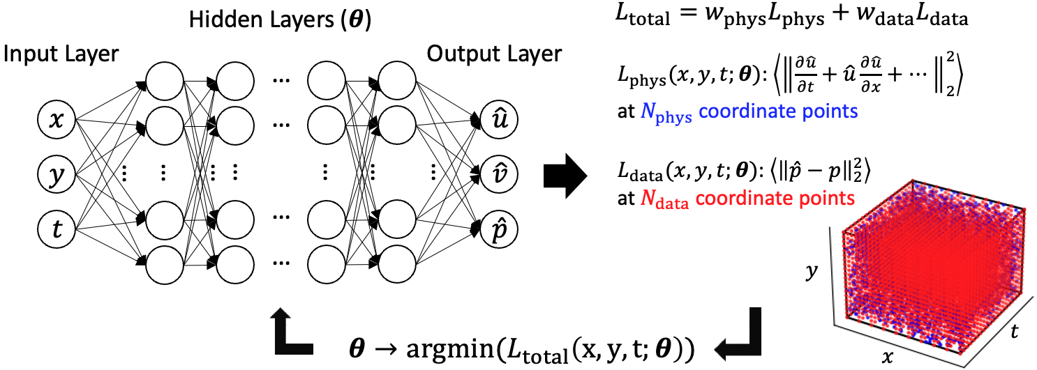
Figure 1: Physics informed neural network for the 2D Navier-Stokes system

2.3 The two-dimensional (2D) Hasegawa-Wakatani system

Next, we consider the 2D Hasegawa-Wakatani system where the time $(t)$ evolution of the density ($n$), the electrostatic potential ($\phi$), and the vorticity ($\Omega$) fields is described by the following equations.

$$0=\frac{\partial n}{\partial t}-c_{1}(\phi-n)+[\phi,n]+\kappa_{n}\frac{\partial\phi}{\partial y}+\nu\nabla^{4}n$$ (7)

$$0=\frac{\partial\Omega}{\partial t}-c_{1}(\phi-n)+[\phi,\Omega]+\nu\nabla^{4}\Omega$$ (8)

$$0=\Omega-\nabla^{2}\phi$$ (9)

where $[a,b]=\frac{\partial a}{\partial x}\frac{\partial b}{\partial y}-\frac{\partial b}{\partial x}\frac{\partial a}{\partial y}$, $c_{1}$ is the adiabatic coefficient taken as 1, $\kappa_{n}$ is the density gradient scale length taken as 1, and $\nu$ is the diffusion coefficient taken as 5e-6. Although this set of equations would not be sufficiently sophisticated to describe fusion plasma turbulence in toroidal geometry, it contains fundamental dynamics and complexity of the drift wave turbulence in fusion plasmas. It can be a minimal test bed for the PINN prediction of turbulent velocity field (the $E\times B$ velocity $\mathbb{v}_{E\times B}=\frac{1}{B^{2}}\mathbb{B}\times\nabla\phi$ where $\mathbb{B}$ is the magnetic field vector) with limited density turbulence measurements.

The equations are numerically solved using a verified Python solver called HW2D [8]. The simulation is run sufficiently long ($t\leq 500$: the nonlinear saturation phase is reached around $t\sim 150$ and the calculation time step $\delta t=0.025$) over the $0\leq x\leq 41.902$ and $0\leq y\leq 41.902$ space with 512 x 512 grid points ($\delta x=\delta y=0.082$), but the domain of interest for the PINN training is restricted as $0\leq x\leq 4.1$, $0\leq y\leq 2.05$, and $309\leq t\leq 321$ due to the limited computational memory.

We presume that only the density measurement is available from the channels distributed regularly in $(x,y)$ space. Measurements are taken with the uniform time interval to construct the density data sets $\{n_{j}\}$ at the $(x,y,t)$ coordinates. Note that the number of channels is varied to investigate the effect of the spatial resolution of diagnostic channels for the reasonable PINN prediction with the fourth-order derivatives in the equations.

The neural network of the same architecture as in the previous case is used: $(\hat{n},\hat{\phi},\hat{\Omega})=\mathrm{NN}(x,y,t;\boldsymbol{\theta})$. It is left for future work to explore the possibility of the improvement by changing the network architecture and relevant hyperparameters.

3 Result

3.1 The two-dimensional (2D) Navier-Stokes system

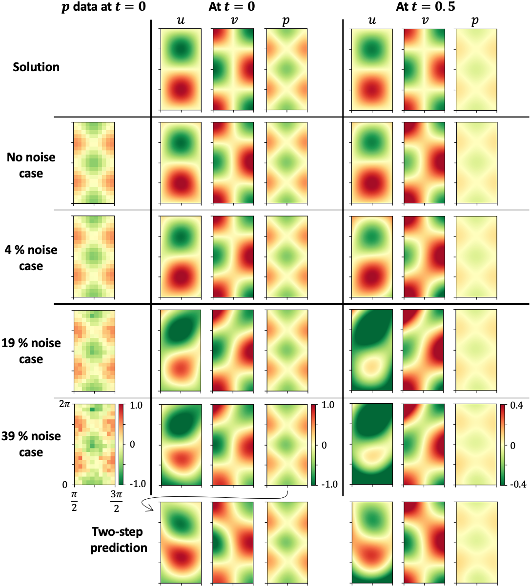
Figure 2: The PINN prediction of the 2D Navier-Stokes system

Results of the PINN prediction of velocity $u$, $v$ and pressure $p$ fields of the 2D Navier-Stokes system are summarized in figure 2. The solutions at two different times $t=0$ and $t=0.5$ are plotted at the top, showing rapidly decaying vortices (the narrower color scales were used at the later time). Each PINN, $(\hat{u},\hat{v},\hat{p})=\mathrm{NN}(x,y,t;\boldsymbol{\theta})$, is trained with the pressure data sets $\{p_{j}\}$ at the same $(x,y,t)$ coordinates including different amount of noise. Examples of the pressure data at $t=0$, with the Gaussian noise of different standard deviations, are shown in the first column. The PINN predictions of $u$, $v$, and $p$ at $t=0$ and $t=0.5$ are shown for different levels of the noise in the corresponding columns and rows (4 % means that the standard deviation of the noise is 4 % of the standard deviation of the pure data).

Figure 2 shows that the PINN can predict the velocity fields with only the pressure data provided thanks to the additional physics information. Obviously, the PINN prediction shows the better agreement with the lower noise level, but it is notable that the results with the 39 % noise level still capture the characteristic vortex structure. As time flows and the vortex decays, the deviation becomes more evident with the larger noise.

The pressure prediction seems to be more robust against the noise than the velocity fields prediction. This implies that we can design a two-step noise-robust PINN prediction of the velocity fields: The first PINN aims to refine the pressure data, and the second PINN predicts the velocity fields with the refined pressure data generated by the first PINN (with the arbitrarily resolution in the $(x,y,t)$ space). The result shown at the bottom of figure 2 corresponds to the two-step PINN prediction using the pressure prediction of the 39 % noise case as the training data of the second PINN. To prevent the second PINN from converging to the same minimum loss point in the parameter hyperspace as the first PINN, the second PINN should be configured slightly differently (it can have different activation function such as the swish function or additional hidden layer). Compared to the result of the 39 % noise case, the two-step prediction clearly shows the improvement, meaning a more noise-robust PINN prediction of velocity fields with the pressure data alone in the 2D Navier-Stokes system.

3.2 The two-dimensional (2D) Hasegawa-Wakatani system

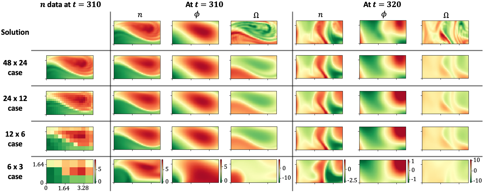
Figure 3: The PINN prediction of the 2D Hasegawa-Wakatani system

Results of the PINN prediction of the density $n$, the electrostatic potential $\phi$ (the $E\times B$ velocity $\mathbb{v}_{E\times B}=\frac{1}{B^{2}}\mathbb{B}\times\nabla\phi$) and the vorticity $\Omega$ fields of the 2D Hasegawa-Wakatani system are shown in figure  3. The solutions at $t=310$ and $t=320$ are plotted at the top, compared with the predictions by the PINNs trained with the density data sets of different spatial resolutions. Each PINN, $(\hat{n},\hat{\phi},\hat{\Omega})=\mathrm{NN}(x,y,t;\boldsymbol{\theta})$, is trained with the density data sets $\{n_{j}\}$ obtained by different number of channels in the $(x,y)$ space. Due to the limited computational memory, the narrower time domain was chosen for the larger channel number case, but the temporal resolution of measurements was kept constant as 5 measurements per $\Delta t=1$. Examples of the density data at $t=310$ are shown in the first column for different channel number cases. The PINN predictions of $n$, $\phi$, and $\Omega$ at two times are shown for different channel number cases in the corresponding columns and rows. The 48 x 24 case means 48 (24) channels are uniformly distributed along $x$ ($y$) direction and separated by $\Delta x=\Delta y=0.089$. Note that the simulation grid step is $\delta x=\delta y=0.082$.

With given only the density measurements, the PINN could capture the key characteristics of the potential (velocity) field down to the 12 x 6 case. Some fine structure in the density field could be reproduced in the 48 x 24 case, but as the number of channels decreases it is lost in the prediction. On the other hand, the fine structure in the vorticity field could not be reproduced at all. Changing the network architecture or renormalizing fields to be on the same scale might be helpful to improve the prediction of the vorticity field.

4 Discussion

The velocity field in a physical system could be predicted by the PINN with other limited data. The pressure or density data was prepared to resemble the actual experimental environment, obtained by the channels distributed in the two-dimensional space and each measurement is separated by the uniform time interval. The effects of the noise is investigated in the 2D Navier-Stokes system. The key characteristics of the velocity field is captured by the PINN even in the 39 % noise case for the time when the vortex does not decay much. In addition, a more noise-robust two-step PINN prediction was introduced. The effects of the channel spatial resolution is investigated in the 2D Hasegawa-Wakatani system. Capturing a finer structure requires the higher spatial resolution of provided data, but the 12 x 6 case already provides almost equivalent prediction to the 48 x 24 case.

Besides the noise and the spatial resolution, the point spread function of the diagnostic channel is another crucial factor that must be taken into account when applying the PINN velocity predictor in practice. Turbulence diagnostics in tokamak plasmas such as beam emission spectroscopy (BES) and electron cyclotron emission imaging (ECEI) utilize optics and analogue/digital filters to obtain a signal whose power depends on plasma fields such as density and temperature in a finite region. In other words, the measured signal of the diagnostic channel contains the integrated information over the finite region. The point spread function of a channel relates local values of plasma fields in the region with the measured signal by the channel. It should be narrow enough not to average out the spatial variation in the structure of interest, but also large enough for the measured signal power not to be buried in noise. Due to effects of the point spread function, the measured signal of a diagnostic channel does not exactly reflect local values of plasma fields which would be ideal for the training of the PINN velocity predictor.

One may consider effects of the point spread function as noise in the data and anticipate that the PINN can predict a velocity field directly using the measured data by diagnostics. Or, one can consider deduction of the plasma fields from the measured data as another inverse problem that can be solved by an artificial neural network. All data sets (the density and temperature field and the corresponding synthetic data of diagnostics) for the training of the network can be freely generated using forward modeling tools [14]. Then, a two-step prediction of the velocity field would be possible: from the measured turbulence data by diagnostics to the density or temperature field and from the density or temperature field to the velocity field. Our work shows that the second step can be facilitated using the PINN with a physics model even with minor errors in the first step.

On the other hand, our work shows that the PINN can inversely identify a solution satisfying physics model equations of a turbulence system with the given measurements, unless the noise is too strong or the spatial resolution of the measurements is insufficient. This implies a way to test model equations with measured turbulence data. Due to the chaotic behavior of turbulence, it was not meaningful to directly compare the observed spatio-temporal dynamics of turbulent structures in experiments with that obtained in the forward calculation of model equations. It is almost impossible to match all the initial and boundary conditions between the experiment and the simulation, and normally the reproducible statistical quantities in the steady state are compared [15]. However, the initial and boundary condition still affect the steady state [16]. By comparing the minimum losses between PINNs trained with the turbulence model synthetic data and the experimentally measured data, it could be decided whether a model is appropriate to describe the evolution of measured plasma field in the experiment or not.

Reference

References

- [1] M. J. Choi, “Spectral data analysis methods for the two-dimensional imaging diagnostics,” arXiv, p. 1907.09184, 2019.
- [2] M. Raissi, A. Yazdani, and G. E. Karniadakis, “Hidden fluid mechanics: Learning velocity and pressure fields from flow visualizations,” Science, vol. 367, no. 6481, p. 1026, 2020.
- [3] Y. W. Enters, S. Thomas, M. Hill, and I. Cziegler, “Testing image-velocimetry methods for turbulence diagnostics,” Review of Scientific Instruments, vol. 94, no. 7, p. 075101, 2023.
- [4] L. Lu, X. Meng, Z. Mao, and G. E. Karniadakis, “DeepXDE: A Deep Learning Library for Solving Differential Equations,” SIAM Review, vol. 63, no. 1, p. 208, 2021.
- [5] G. Taylor, “LXXV. On the decay of vortices in a viscous fluid,” Philosophical Magazine Series 6, vol. 46, no. 274, p. 671, 1923.
- [6] H. Wang, Y. Liu, and S. Wang, “Dense velocity reconstruction from particle image velocimetry/particle tracking velocimetry using a physics-informed neural network,” Physics of Fluids, vol. 34, no. 1, p. 017116, 2022.
- [7] A. Hasegawa and M. Wakatani, “Plasma Edge Turbulence,” Physical Review Letters, vol. 50, no. 9, p. 682, 1983.
- [8] R. Greif, “HW2D: A reference implementation of the Hasegawa-Wakatani model for plasma turbulence in fusion reactors,” Journal of Open Source Software, vol. 8, no. 92, p. 5959, 2023.
- [9] J. Seo, “Solving real-world optimization tasks using physics-informed neural computing,” Scientific Reports, vol. 14, no. 1, p. 202, 2024.
- [10] A. Mathews, M. Francisquez, J. W. Hughes, D. R. Hatch, B. Zhu, and B. N. Rogers, “Uncovering turbulent plasma dynamics via deep learning from partial observations,” Physical Review E, vol. 104, no. 2, p. 025205, 2021.
- [11] M. Abadi, P. Barham, J. Chen, Z. Chen, A. Davis, J. Dean, M. Devin, S. Ghemawat, G. Irving, M. Isard, M. Kudlur, J. Levenberg, R. Monga, S. Moore, D. G. Murray, B. Steiner, P. Tucker, V. Vasudevan, P. Warden, M. Wicke, Y. Yu, and X. Zheng, “Tensorflow: a system for large-scale machine learning,” in Proceedings of the 12th USENIX Conference on Operating Systems Design and Implementation, OSDI’16, (USA), p. 265, USENIX Association, 2016.
- [12] T. Tieleman, “Lecture 6.5‐rmsprop: Divide the gradient by a running average of its recent magnitude,” COURSERA: Neural networks for machine learning, vol. 4, no. 2, p. 26, 2012.
- [13] J. F. Bonnans, J. C. Gilbert, C. Lemaréchal, and C. A. Sagastizáchal, Numerical Optimization: Theoretical and Practical Aspects. Universitext, Heidelberg: Springer Berlin, 2 ed., 2006.
- [14] M. J. Choi, “syndia: First release,” Apr. 2022.
- [15] M. J. Choi, J.-M. Kwon, L. Qi, P. H. Diamond, T. S. Hahm, H. Jhang, J. Kim, M. Leconte, H.-S. Kim, J. Kang, B.-H. Park, J. Chung, J. Lee, M. Kim, G. S. Yun, Y. U. Nam, J. Kim, W.-H. Ko, K. D. Lee, J. W. Juhn, and t. K. Team, “Mesoscopic transport in KSTAR plasmas: avalanches and the E × B staircase,” Plasma Physics and Controlled Fusion, vol. 66, no. 6, p. 065013, 2024.
- [16] G. Dif-Pradalier, P. Ghendrih, Y. Sarazin, E. Caschera, F. Clairet, Y. Camenen, P. Donnel, X. Garbet, V. Grandgirard, Y. Munschy, L. Vermare, and F. Widmer, “Transport barrier onset and edge turbulence shortfall in fusion plasmas,” Communications Physics, vol. 5, no. 1, p. 229, 2022.