Optimal and Feasible Contextuality-based Randomness Generation

Abstract

Semi-device-independent (SDI) randomness generation protocols based on Kochen-Specker contextuality offer the attractive features of compact devices, high rates, and ease of experimental implementation over fully device-independent (DI) protocols. Here, we investigate this paradigm and derive four results to improve the state-of-art. Firstly, we introduce a family of simple, experimentally feasible orthogonality graphs (measurement compatibility structures) for which the maximum violation of the corresponding non-contextuality inequalities allows to certify the maximum amount of $\log_{2}d$ bits from a qu$d$it system with projective measurements for $d\geq 3$. We analytically derive the Lovasz theta and fractional packing number for this graph family, and thereby prove their utility for optimal randomness generation in both randomness expansion and amplification tasks. Secondly, a central additional assumption in contextuality-based protocols over fully DI ones, is that the measurements are repeatable and satisfy an intended compatibility structure. We frame a relaxation of this condition in terms of $\epsilon$-orthogonality graphs for a parameter $\epsilon>0$, and derive quantum correlations that allow to certify randomness for arbitrary relaxation $\epsilon\in[0,1)$. Thirdly, it is well known that a single qubit is non-contextual, i.e., the qubit correlations can be explained by a non-contextual hidden variable (NCHV) model. We show however that a single qubit is almost contextual, in that there exist qubit correlations that cannot be explained by $\epsilon$-faithful NCHV models for small $\epsilon>0$. Finally, we point out possible attacks by quantum and general consistent (non-signalling) adversaries for certain classes of contextuality tests over and above those considered in DI scenarios.

Introduction.– Contextuality is a defining feature of quantum theory, distinguishing it from classical (non-contextual) hidden variable theories. The phenomenon of contextuality (specifically Kochen-Specker contextuality aka outcome contextuality) shows that outcomes cannot be assigned to quantum measurements (in Hilbert spaces of dimension $d\geq 3$) independently of the particular contexts in which the measurements are realized. The fact that the measurements of quantum observables may not be thought of as revealing pre-determined properties implies a fundamental or intrinsic randomness that can be exploited in quantum randomness expansion and amplification protocols ekert1991quantum ; herrero2017quantum . Such protocols offer the promise of high-quality quantum-certified secure random bits that would be crucial for several cryptographic protocols.

While fully device-independent (DI) protocols based on tests of quantum nonlocality have been developed in recent years for the tasks of randomness generation, expansion and amplification pironio2010random ; pironio2013security ; brown2019framework ; liu2021device ; colbeck2012free ; gallego2013full ; ramanathan2016randomness ; brandao2016realistic ; ramanathan2018practical ; kessler2020device ; zhao2022tilted ; ramanathan2021no ; ramanathan2023finite , their experimental implementation is highly demanding, with the requirement of high-fidelity entanglement distributed between multiple devices and high detection efficiencies. In contrast, contextuality can be tested in a single quantum system, which significantly simplifies the experimental requirements to observe the violation of non-contextuality inequalities. The price to pay however is the additional assumption that the measurements obey specified compatibility relations and each measurement does not influence the marginal distribution of outcomes of compatible measurements. As such, contextuality-based protocols are said to be semi-device-independent (SDI), note however that other than these basic assumptions, no other assumption is required on the state, measurements or dimension of the system. The SDI framework thus offers a practical compromise between security and feasibility, allowing for compact, experimentally feasible high-rate protocols.

While multiple investigations of contextuality-based SDI protocols have been carried out in recent years abbott2012strong ; abbott2014value ; abbott2015variant ; um2020randomness ; um2013experimental ; singh2017quantum ; singh2024local ; ramanathan2020gadget ; liu2023optimal , several fundamental open questions remain. Is there a contextuality test that certifies the maximum theoretical amount of $\log_{2}d$ bits from projective measurements on a $d$-dimensional quantum system for arbitrary $d\geq 3$ acin2016optimal ; borkala2022device ; sarkar2023self ; farkas2024maximal , in the practical experimental situation where the measurements are chosen using weakly random seeds, where the measurements are non-ideal and under a relaxation of the assumption that the measurements conform to a specified compatibility structure? It is well-known that experiments can only refute non-contextual hidden variable (NCHV) models that are $\epsilon$-faithful, meaning that quantum effects that are $\epsilon$-close can only be assigned different values in the NCHV model with $\epsilon$ probability. Can all quantum correlations be explained by $\epsilon$-faithful NCHV models for some threshold value of $\epsilon$, or can quantum theory refute such models for arbitrary $\epsilon$? It is well known that a single qubit is non-contextual since its correlations can be explained by a NCHV model. However, since only $\epsilon$-faithful NCHV models can be refuted in any experiment, could a single qubit system be $\epsilon$-contextual and thereby still be useful for some tasks? Finally, what kind of attacks can be carried out by an adversary holding quantum (or more general non-signalling) correlations on contextuality-based SDI protocols over and above those in the fully device-independent setting?

In this paper, we answer the above fundamental questions paving the way for practical realizations of optimal contextuality-based protocols. We first introduce a family of measurement structures (represented as orthogonality graphs) and a family of non-contextuality inequalities parametrised by dimension $d\geq 3$ and derive their maximal value in NCHV, quantum and general consistent or non-disturbing theories. We prove that observing the maximum quantum violation of these inequalities certifies $\log_{2}d$ bits of randomness, and that furthermore the certification is possible even when the measurements are chosen with an arbitrarily weak source of randomness. We then revisit the notion of $\epsilon$-ontologically faithful NCHV models (so-called $\epsilon$-ONC models) introduced by Winter winter2014does for the practical situation wherein one cannot distinguish precisely between a projector and an arbitrarily close POVM element. We derive a tight bound on the value achieved by $\epsilon$-ONC models for general non-contextuality inequalities and use it to show that quantum theory cannot be explained by such models for arbitrary $\epsilon\in[0,1)$. Thirdly, we prove that a single qubit is almost contextual in that there exist qubit correlations that cannot be explained by $\epsilon$-ONC models for a small parameter $\epsilon>0$. Finally, we investigate the security of contextuality-based protocols by deriving a class of attacks when certain tests of contextuality are used, by both quantum and general non-signalling adversaries.

Certifying $\log_{2}d$ bits of randomness from qudit systems for $d\geq 3$.– In a randomness generation protocol, the optimal amount of randomness that can be certified from a qu$d$it system using projective measurements is $\log_{2}d$. We introduce a family of non-contextuality inequalities for each dimension $d\geq 3$ to achieve this optimal value. More precisely, we show that when the maximum quantum values of these non-contextuality expressions are achieved, one of the measurement setttings necessarily yields $d$ outcomes each occurring with uniform probability $1/d$.

The corresponding measurement structures are illustrated in Fig. 1 as orthogonality graphs. Specifically, the measurement structure in dimension $d$ is defined by a finite set consisting of $5\cdot d$ rank-one projectors $S_{d}=\{|v_{i,j}\rangle\langle v_{i,j}|\}_{i=1,\ldots,d;j=1,\ldots,5}$. The projectors exhibit the following orthogonality structure: (1) projectors in $\{|v_{i,1}\rangle\langle v_{i,1}|\}_{i=1}^{d}$ are mutually orthogonal, and (2) for each $i\in\{1,\ldots,d\}$, the projector $|v_{i,j}\rangle\langle v_{i,j}|$ is orthogonal to $|v_{i,j+1}\rangle\langle v_{i,j+1}|$ with $j+1$ taken modulo $5$. The corresponding orthogonality graph $\mathcal{G}_{d}=(\mathcal{V}_{d},\mathcal{E}_{d})$ is drawn with each vertex in $\mathcal{V}_{d}$ representing a projector in $S_{d}$ and two vertices connected by an edge if and only if the corresponding projectors are orthogonal. From the orthogonality relations among the projectors in $S_{d}$, we see that the orthogonality graph $\mathcal{G}_{d}$ contains a central maximum clique of size $d$ along with $d$ cycles of length $5$ ($C_{5}$), with every vertex in the maximum clique associated with a single $C_{5}$.

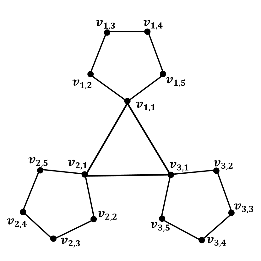
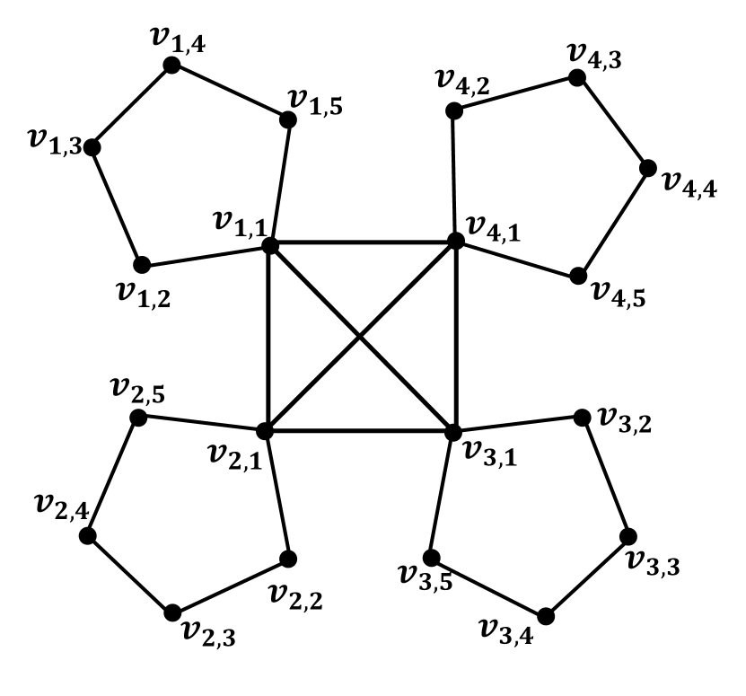
Figure 1: The orthogonality graphs $\mathcal{G}_{3}$, $\mathcal{G}_{4}$ for rank-one projector sets $S_{3}$ and $S_{4}$ described in the main text.

From the set of projectors, one can also construct a set of binary observables defined by $A_{i,j}:=\mathbb{I}-2|v_{i,j}\rangle\langle v_{i,j}|$, with eigenvalues $\{+1,-1\}$, whose compatibility structure follows directly from the orthogonality relations of the projectors. Compatible observables can, in principle, be jointly measured, and their measurement outcomes in quantum theory are unaffected by the order in which they are measured. We now present the following non-contextuality expression $\mathcal{I}_{d}$ for any $d\geq 3$, ensuring that each term (referring to one context) in $\mathcal{I}_{d}$ consists of compatible observables:

$$\mathcal{I}_{d}:=2\prod_{i=1}^{d}A_{i,1}+\sum_{i=1}^{d}\sum_{j=1}^{5}A_{i,j}A_{i,j+1}$$ (1)

The non-contextual hidden variable (NCHV) bound and quantum bound of the above non-contextuality expression are directly related to the weighted independence number and Lovász theta number of the orthogonality graph. To be precise, we rewrite the expression $\mathcal{I}_{d}$ using the orthogonality relations as:

$$\begin{split}\mathcal{I}_{d}&=2\mathbb{I}-4\sum_{i=1}^{d}|v_{i,1}\rangle\langle v_{i,1}|+\sum_{i=1}^{d}\left(5\mathbb{I}-4\sum_{j=1}^{5}|v_{i,j}\rangle\langle v_{i,j}|\right)\\ &=(5d+2)\mathbb{I}-4\sum_{i=1}^{d}\left(2|v_{i,1}\rangle\langle v_{i,1}|+\sum_{j=2}^{5}|v_{i,j}\rangle\langle v_{i,j}|\right).\end{split}$$ (2)

The NCHV lower bound for the expectation value of $\mathcal{I}_{d}$ is calculated based on all possible $\{0,1\}$non-contextual assignments for projectors in $S_{d}$, which is equivalent to the weighted independence number of the orthogonality graph $\mathcal{G}_{d}$, with weight $2$ assigned to vertices $v_{i,1}\ \forall i$ and weight $1$ to the other vertices. Denote this set of weights to the vertices of the graph by $\bm{w}$. Quantum theory allows to achieve a value lower than the NCHV bound, characterized by the weighted Lovász theta number of the orthogonality graph $\mathcal{G}_{d}$ (given by a semidefinite program). In general consistent (no-disturbance) theories, the value of the non-contextuality expression is characterized in terms of the weighted fractional packing number $\alpha^{*}(\mathcal{G}_{d},\bm{w})$ (given by a linear program). See App. A for a brief explanation of these parameters in relation to quantum contextuality.

$$\langle\mathcal{I}_{d}\rangle\overset{\text{NCHV}}{\geq}(5d+2)-4\alpha(\mathcal{G}_{d},\bm{w})\overset{\text{Q}}{\geq}(5d+2)-4\theta(\mathcal{G}_{d},\bm{w}).$$ (3)

$d$	3	4	5	6	7	8	$d\geq 9$
$\alpha^{*}(\mathcal{G}_{d},\bm{w})$	8	10	12	14	16	18	$2d+2$
$\theta(\mathcal{G}_{d},\bm{w})$	7.6753	9.8030	11.8869	13.9419	15.9762	17.9944	$2d+2$
$\alpha(\mathcal{G}_{d},\bm{w})$	7	9	11	13	15	17	$2d+1$

Table 1: The weighted fractional packing number, weighted independence number and weighted Lovász theta number of the orthogonality graphs $\mathcal{G}_{d}$.

The NCHV, quantum and no-disturbance (consistent) lower bounds of the non-contextual expression $\mathcal{I}_{d}$ are given by the values in Table 1. Furthermore, we also show that any quantum correlation achieving $\theta(\mathcal{G}_{d},\bm{w})$ necessarily yields uniform probabilities $1/d$ for the central clique, for arbitrary $d\geq 3$. In particular, we show the following (proof in Appendix B).

Theorem 1.

The weighted independence number of the graph $\mathcal{G}_{d}$ is $\alpha(\mathcal{G}_{d},\bm{w})=2d+1$ for any $d\geq 3$, where vertices $v_{i,1}\ \forall i$ are assigned weight $2$ and all other vertices are assigned weight $1$. The weighted Lovász theta number for these weights is $\theta(\mathcal{G}_{d},\bm{w})=2d+2$ for $d\geq 9$, with the value for $3\leq d\leq 8$ being given as in the Table 1. The weighted fractional packing number is $\alpha^{*}(\mathcal{G}_{d},\bm{w})=2d+2$ for $d\geq 3$. Furthermore, for any quantum correlation achieving the weighted Lovász theta number, there exists a measurement setting (a context) $c^{*}$ that produces $d$ outcomes, each occurring with a uniform probability of $1/d$.

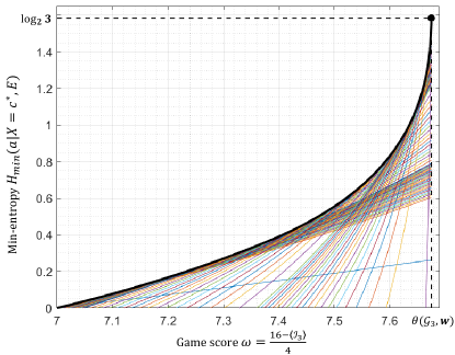
Figure 5: The min-entropy $H_{\text{min}}(a|X=c^{*},E)$ versus the game score $\omega:=\frac{(5d+1)-\langle\mathcal{I}_{d}\rangle}{4}$ curve for $d=3$ with a family of min-tradeoff functions.

Use in randomness expansion and amplification.– The above contextuality tests may be used in SDI randomness expansion protocols brown2019framework wherein the task is to expand a short fully random seed into a larger string of uniformly random bits. The Entropy Accumulation Theorem (EAT) provides a lower bound on the total output randomness for the protocol. We give the detailed description of the protocol in the App. F where we review the definition of EAT channels  arnon2018practical ; dupuis2020entropy , adapting them to the contextuality scenario. Note that at this stage, we assume that the observables satisfy the intended compatibility structure. In the next section, we show how the tests certify randomness even when this assumption is relaxed. We plot the randomness quantified by the min-entropy $H_{\text{min}}(a|X=c^{*},E)$ as a function of the game score $\omega:=\frac{(5d+2)-\langle\mathcal{I}_{d}\rangle}{4}$ for $d=3$ in Figure 5. As can be seen, the observation of the maximum value $\theta(\mathcal{G}_{d},\bm{w})$ certifies $\log_{2}3$ bits of randomness. We also remark on the simplicity of the orthogonality graph and the noise tolerance of the resulting inequality, features that make these tests suitable for optimal randomness expansion. Additionally, we plot a family of convex, differentiable functions $\{f_{\hat{\omega}}(\omega)\}_{\hat{\omega}}$ as candidates for the min-tradeoff function in the protocol. After selecting the parameter $\omega_{exp}$, an appropriate function from this family should be applied as $f_{\text{min}}$ in the protocol to lower bound the total randomness (see App. F).

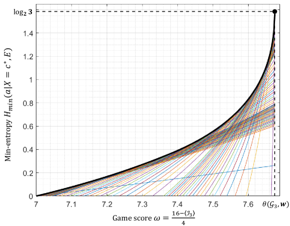
Figure 2: The min-entropy $H_{\text{min}}(a|X=c^{*},E)$ (and a family of min-tradeoff functions) versus the game score $\omega:=\frac{(5d+2)-\langle\mathcal{I}_{d}\rangle}{4}$ for $d=3$.

Finally, we note that the derived non-contextuality inequalities also make ideal candidates for randomness amplification protocols colbeck2012free ; gallego2013full ; ramanathan2016randomness ; brandao2016realistic ; ramanathan2018practical ; kessler2020device ; zhao2022tilted ; ramanathan2021no ; ramanathan2023finite . In this class of protocols, one starts with a weak seed such as a Santha-Vazirani source where each bit has a small amount of randomness defined by $0\leq\kappa<1/2$ conditioned on any adversarial side information. That is, we have $1/2-\kappa\leq\text{Pr}[X_{j}=0|X_{0},X_{1},\ldots,X_{j-1}]\leq 1/2+\kappa$ for all $j$. The task of randomness amplification is to extract private, fully random bits from such a weakly random source. It is well-known that in order to achieve randomness amplification from sources of arbitrary $\kappa<1/2$, one requires quantum correlations that achieve (or get arbitrary close to) the general consistent (non-signalling) bound for the test. The fact that the derived inequalities certify the maximum amount of $\log_{2}d$ bits for $d\geq 9$ under the condition that $\alpha(\mathcal{G}_{d},\bm{w})<\theta(\mathcal{G}_{d},\bm{w})=\alpha^{*}(\mathcal{G}_{d},\bm{w})$ thus make them ideal candidates for this task.

In this regard, it is important to note that not all contextuality tests are useful for randomness expansion and amplification (see App. G). Indeed, one can devise attacks by quantum adversaries (who share quantum correlations with the device implementing the protocol) on protocols that are only based on the observed value of a state-independent contextuality inequality. Furthermore, for the specific class of parity proofs based on magic arrangements which include the famous Peres-Mermin magic square and the Mermin star, one can devise attacks by hybrid classical adversaries who share only classical correlations with the device but are allowed to prepare general consistent behaviors for the device.

Relaxed $\epsilon$-Non-Contextuality for Experimental Feasibility.– The central additional assumption made in our SDI protocols in contrast to fully device-independent protocols is that of non-contextuality, the idea that the “same” projector is measured in multiple contexts. That is, an outcome i in one measurement and an outcome j in another measurement (which may require completely different experiments) are identified with each other. In particular, we assume in the NCHV model that the random variables $f_{i},f_{j}\in\{0,1\}$ associated to these outcomes are identical. Similarly, in the quantum model, we assume that the associated projectors (or more generally POVM elements or quantum effects) are identical. For practical contextuality experiments (and the resulting SDI protocols), this is clearly not feasible since experiments cannot distinguish perfectly between a projector $P_{i}$ and an arbitrarily close POVM element $Q_{i}$ (a positive semidefinite operator $\leq\textbf{1}$). The general NCHV model though may assign different values ($0$ and $1$) to arbitrarily close quantum effects, so that one has a “nullification” of the Bell-Kochen-Specker argument. Indeed, Meyer, Clifton and Kent meyer1999finite ; kent1999noncontextual ; clifton2000simulating have provided such a nullification, by showing that for each $d\geq 3$ there exists a dense set of complete projective measurements consisting of rank-one projectors, with the property that every projector occurs in only one measurement. As such, in actual experimental situations and SDI protocols, we do not certify quantum contextuality against arbitrary NCHV models but are forced to consider so-called $\epsilon$-ontologically faithful non-contextual models for a parameter $\epsilon\in[0,1)$, formally introduced by Winter in winter2014does . Here, we adapt the definition for orthogonality graphs, give a tighter upper bound for non-contextuality inequalities than considered in winter2014does , and use it to show that quantum contextuality can be certified for arbitrary $\epsilon$.

Definition 1.

An $\epsilon$-ontologically faithful non-contextual ($\epsilon$-ONC) model for an orthogonality graph $G=(V,E)$ with maximal clique set $\Gamma$ consists of a family of random variables $f_{v}^{C}\in\{0,1\}$ for vertices $v\in V$ and contexts $C\in\Gamma$ such that

$$\sum_{v\in C}f_{v}^{C}\leq 1,\quad\forall C\in\Gamma,$$

$$\text{Pr}\left[f_{v}^{C}\neq f_{v}^{C^{\prime}}\right]\leq\epsilon,\quad\forall C,C^{\prime}\in\Gamma,\;\forall v\in C\cap C^{\prime}.$$ (4)

In other words, in the relaxed NCHV model, we treat the observable corresponding to vertex $v$ appearing in different contexts $C$ and $C^{\prime}$ as almost identical, i.e., the probability that the corresponding random variables $f_{v}^{C}$ and $f_{v}^{C^{\prime}}$ are assigned different values $0$ and $1$ is at most $\epsilon$. We give a graph-theoretic representation for the above model and refine the upper bound on the maximum value of a non-contextuality inequality in such $\epsilon$-ONC models. To incorporate $\epsilon$-orthogonality, we construct from a given orthogonality graph $G$ a new $\epsilon$-orthogonality graph with additional $\epsilon$-edges. While normal edges indicate strict orthogonality, an $\epsilon$-edge indicates that the quantum effects are “almost” orthogonal.

Definition 2.

An $\epsilon$-orthogonality graph $G_{\epsilon}$ for a set $V$ is defined as a triple $G_{\epsilon}=(V,E,\widetilde{E}_{\epsilon})$, where $V$ is the set of vertices, $E$ is the normal edge set representing strict orthogonality, and $\widetilde{E}_{\epsilon}$ is the $\epsilon$-edge set representing $\epsilon$-orthogonality.

In a graph two vertices connected by a normal edge have zero “independence”, they cannot belong to the same independent set. On the other hand, non-adjacent vertices have complete “independence”. $\epsilon$-edges offer an intermediate level of independence between two vertices. This translates into the idea that the probability that two purportedly orthogonal projectors are both assigned value $1$ is at most $\epsilon$.

We now proceed to calculate the maximum value in $\epsilon$-ONC models of a non-contextuality inequality with uniform weights for a given orthogonality graph $G=(V,E)$. From the given graph $G$, we construct an $\epsilon$-orthogonality graph $G_{\epsilon}$ with weights w depending on the number of contexts each projector is measured in, and calculate the maximum value as $\alpha_{\epsilon}(G_{\epsilon},\textbf{w})$. To do this, we define two related normal graphs: $G^{\prime}_{\epsilon}=(V,E)$, which includes only the normal edges of $G_{\epsilon}$ (and is thus just a bunch of disjoint maximal cliques), and $G^{\prime\prime}_{\epsilon}=(V,E\cup\widetilde{E}_{\epsilon})$, which treats the $\epsilon$-edges as normal edges. We show in App. C that

$$\alpha_{\epsilon}(G_{\epsilon},\textbf{w})=\epsilon\cdot\alpha(G^{\prime}_{\epsilon},\textbf{w})+(1-\epsilon)\cdot\alpha(G^{\prime\prime}_{\epsilon},\textbf{w}).$$ (5)

This parameter is the solution to an integer program:

$$\begin{split}\alpha_{\epsilon}(G_{\epsilon},\bm{w}):=\max_{\bm{x},\bm{y}}&\quad\epsilon\cdot\bm{w}^{T}\bm{x}+(1-\epsilon)\cdot\bm{w}^{T}\bm{y}\\ \text{s.t.}&\quad x_{i}+x_{j}\leq 1\quad\forall(i,j)\in E,\\ &\quad y_{i}+y_{j}\leq 1\quad\forall(i,j)\in E\cup\widetilde{E}_{\epsilon},\\ &\quad x_{i},y_{i}\in\{0,1\}\quad\forall i\in V.\end{split}$$ (6)

Having established the value of non-contextuality inequalities under the experimentally testable $\epsilon$-ONC models, we now show that there exist quantum correlations that exceed this value for certain inequalities for arbitrary value of $\epsilon\in[0,1)$.

Theorem 2.

There exist non-contextuality inequalities and corresponding optimal quantum correlations that certify contextuality against $\epsilon$-ONC models, for arbitrary $\epsilon\in[0,1)$.

We prove this theorem (details are in Appendix C) by showing that the threshold $\epsilon$ for orthogonality graphs correspond to odd cycles $C_{n}$ is given by $\epsilon\leq 1-\frac{\pi^{2}}{4n}$. Therefore, for any $\epsilon\in[0,1)$, the optimal quantum correlations for the odd cycle $C_{n}$ with odd $n\geq\left\lceil\frac{\pi^{2}}{4(1-\epsilon)}\right\rceil$, serve to certify contextuality.

$\epsilon$-Contextuality for a single Qubit system.– It has long been known that a single qubit is non-contextual, the KS theorem only applies to Hilbert spaces of dimension $\geq 3$ and an explicit NCHV model has been derived to explain the correlations in a single qubit kochen1990problem ; bell1966problem . Some arguments for qubit contextuality exist cabello2003kochen , but these use POVMs instead of projectors grudka2008there . On the other hand, as we have seen above, experimentally we only refute $\epsilon$-ONC models. In this latter class of models, we consider that projectors that are $\epsilon$-close (in a measure such as operator norm) are assigned different values with probability at most $\epsilon$. We have also seen that the maximum value of a non-contextuality inequality under $\epsilon$-ONC models is given by the epsilon independence number of a corresponding graph $G_{\epsilon}$.

While the graph $G_{\epsilon}$ is intended to capture near-orthogonalities due to inevitable experimental imperfections, one can also ask for the theoretical maximum value attained by quantum correlations under such near-orthogonalities. One can correspondingly write the $\epsilon$-Lovász theta number associated with an orthogonal representation of the graph that allows vectors corresponding to vertices connected by $\epsilon$-edges to have an overlap quantified by $\epsilon$.

$$\begin{split}\theta_{\epsilon}(G_{\epsilon},\bm{w}):=\max_{|\psi\rangle,\{|v_{i}\rangle\}}&\quad\sum_{i\in V}w_{i}|\langle\psi|v_{i}\rangle|^{2}\\ \text{subject to:}&\quad\||\psi\rangle\|^{2}=1,\||v_{i}\rangle\|^{2}=1,\forall i\in V,\\ &\quad\langle v_{i}|v_{j}\rangle=0,\forall(i,j)\in E,\\ &\quad|\langle v_{p}|v_{q}\rangle|\leq\epsilon,\forall(p,q)\in\widetilde{E}_{\epsilon},\end{split}$$ (7)

This parameter is effectively bounded by the solution of an SDP relaxation of the optimization problem in Eq. (6) (proof in App. D).

Lemma 1.

For any $\epsilon$-graph $G_{\epsilon}$ with vertex weights $\bm{w}$, the $\epsilon$-Lovász theta number is lower-bounded by the SDP relaxation of the $\epsilon$-independence number, i.e., $\theta_{\epsilon}(G_{\epsilon},\bm{w})\geq\theta^{\prime}_{\epsilon}(G_{\epsilon},\bm{w})$, where

$$\begin{split}\theta^{\prime}_{\epsilon}(G_{\epsilon},\bm{w}):=\max_{X,Y}&\quad\epsilon\cdot(\sqrt{\bm{w}}^{T}X\sqrt{\bm{w}})+(1-\epsilon)\cdot(\sqrt{\bm{w}}^{T}Y\sqrt{\bm{w}})\\ \text{s.t.}&\quad X_{ij}=0,\;\;\forall(i,j)\in E,\\ &\quad Y_{ij}=0,\;\;\forall(i,j)\in E\cup\widetilde{E}_{\epsilon},\\ &\quad X_{ii}=Y_{ii},\;\;\forall i\in V,\\ &\quad\operatorname{Tr}(X)=1,\;\;\operatorname{Tr}(Y)=1,\\ &\quad X\succeq 0,\;\;Y\succeq 0.\end{split}$$ (8)

Now interestingly, the above $\epsilon$-orthogonality relations enable non-trivial $\epsilon$-orthogonality graph structures in qubit systems. Indeed, we use it to show that for any $\epsilon\in(0,\frac{1}{\sqrt{2}})$, qubit systems with projective measurements exhibit $\epsilon$-contextuality (details in Appendix E). That is, for these values of $\epsilon$, one can find graphs $G_{\epsilon}$ and weights $\bm{w}$ such that $\theta_{\epsilon}(G_{\epsilon},\bm{w})>\alpha_{\epsilon}(G_{\epsilon},\bm{w})$.

Theorem 3.

There exist non-contextuality inequalities and corresponding qubit correlations that certify quantum contextuality against $\epsilon$-ONC models for $\epsilon\in(0,\frac{1}{\sqrt{2}})$, thereby exhibiting $\epsilon$-contextuality for a qubit.

Conclusions and Open Questions.– In this paper, we have derived a family of contextuality tests to certify the maximum possible amount of $\log d$ bits of randomness from $d$-dimensional quantum systems. The tests are experimentally feasible and incorporate practical constraints including measurement settings being chosen with arbitrarily weak random seeds and a relaxation of the assumption that the measurements exactly conform to a prescribed compatibility structure. We have also seen that in this practical situation, even a single qubit is almost contextual, thereby introducing a possibility of utilising single qubit systems in contextuality applications. A few open questions still remain. The first is to implement the prescribed tests in an actual experimental protocol and identify the advantage in rates and detection efficiency over other implementations such as those based on self-testing singh2024local . The second is to establish, in the tradition of contextuality investigations, the minimum orthogonality graphs that certify $\log d$ bits for arbitrary $d\geq 3$, and identify ones that give the best tolerance to noise, weak seeds and relaxations of the classical non-contextual model. For this purpose, it would be useful to identify graphs such that their Lovasz theta equals the fractional packing number, for which constructive methods have been developed based on local complementation orbits cabello2013exclusivity .

Additional references cited in the Appendix: cabello2014graph ; milgrom2002envelope ; lovasz1979shannon ; renner2004smooth ; navascues2007bounding ; navascues2008convergent ; yu2012state ; arkhipov2012extending .

Acknowledgments.– We acknowledge support from the General Research Fund (GRF) Grant No. 17211122, and the Research Impact Fund (RIF) Grant No. R7035-21.

Appendix A Kochen-Specker contextuality

Quantum contextuality is a foundational feature of quantum mechanics that challenges classical explanations of nature by rejecting non-contextual hidden-variable (NCHV) models. In quantum mechanics, a projective measurement $M$ consists of a set of orthogonal projectors $M=\{P_{1},P_{2},\ldots\}$, where each projector satisfies $P_{i}P_{j}=\delta_{ij}P_{i}$ and $\sum_{i}P_{i}=\mathbb{I}$. Each projector $P_{i}$ represents an outcome $i$ of the measurement $M$, and the probability of obtaining this outcome $i$ when measuring $M$ on a quantum state $|\psi\rangle$ is given by $p_{\psi}(i|M)=\langle\psi|P_{i}|\psi\rangle$. If distinct projective measurements $M$ and $M^{\prime}$ share the same projector $P$, the outcome probabilities for $P$ when testing these two measurements on the same state $|\psi\rangle$ are identical and equal to $\langle\psi|P|\psi\rangle$. This implies a form of non-contextuality in quantum measurements: the probabilities of measurement outcomes depend only on the projectors themselves (and the state being tested) rather than the specific measurement context to which the projectors belong.

Classical theory attempts to explain this quantum phenomenon through hidden-variable models that obey the non-contextual feature. Non-contextual hidden-variable (NCHV) models assume the existence of hidden variables $\lambda$ (with an associated distribution) that predetermine measurement outcomes, such that the probability of measuring $M$ and obtaining outcome $i$ can be expressed as

$$p_{\psi}(i|M)=\sum_{\lambda}q_{\psi}(\lambda)f_{\lambda}(i),$$ (9)

where $q_{\psi}(\lambda)>0$ and $\sum_{\lambda}q_{\psi}(\lambda)=1$ is the probability distribution of hidden variables $\lambda$ associated with the state $|\psi\rangle$. The response function $f_{\lambda}$ is defined over the projectors $\{P_{i}\}$, regardless of the measurement context to which each $P_{i}$ belongs, and satisfies $f_{\lambda}(i)\in\{0,1\}$ with $\sum_{i,P_{i}\in M}f_{\lambda}(i)=1$.

The conflict between quantum contextuality and NCHV models was studied by Bell, Kochen and Specker, who focused on the infeasibility of defining a response function $f_{\lambda}$ that exhibits non-contextual properties. Specifically, the Kochen-Specker (KS) theorem kochen1990problem states that there exists a finite set of vectors (rank-one projectors) $\mathcal{V}=\{|v_{1}\rangle,\ldots,|v_{n}\rangle\}\subset\mathbb{C}^{d}$ in a $d$-dimensional Hilbert space for $d\geq 3$ for which it is impossible to find a $\{0,1\}$-assignment function $f:\mathcal{V}\rightarrow\{0,1\}$ satisfying:

1. Exclusivity condition: $f(|v\rangle)+f(|v^{\prime}\rangle)\leq 1$ for any two orthogonal vectors $|v\rangle$ and $|v^{\prime}\rangle$;

2. Completeness condition: $\sum_{|v\rangle\in C\subset\mathcal{V}}f(|v\rangle)=1$ for every size $d$ ($|C|=d$) mutually orthogonal vectors $C$ set.

The set $\mathcal{V}$ that satisfies these properties is referred to as a KS set or a proof of the KS theorem.

Reasoning about quantum contextuality has traditionally been approached using graph-theoretic representations. For any set of vectors $\mathcal{V}$, one can define an orthogonality graph $G$, where each vector $|v\rangle\in\mathcal{V}$ corresponds to a vertex $v$ in $G$, and two vertices $v_{1},v_{2}$ are connected by an edge if and only if $\langle v_{1}|v_{2}\rangle=0$. The feasibility of the $\{0,1\}$-assignment problem for a given set of vectors can then be formulated as the problem of $\{0,1\}$-coloring its orthogonality graph. A $\{0,1\}$-coloring of a graph $G$ is a map $f:V_{G}\rightarrow\{0,1\}$ that satisfies:

1. For every clique $C$ in $G$, it holds that $\sum_{v\in C}f(v)\leq 1$;

2. For every maximal clique $C$ in $G$ of size $\omega(G)$, there exists exactly one vertex $v\in C$ such that $f(v)=1$.

Here, $V_{G}$ denotes the vertex set of $G$, a clique is a set of mutually adjacent vertices, and $\omega(G)$ is the size of the largest clique in $G$.

For a given orthogonality graph $G$, we can label each vertex $v_{i}$ as an input-output event $(v_{i}|C_{v_{i}})$, where $C_{v_{i}}$ is a clique containing vertex $v_{i}$. By interpreting orthogonality between vertices as exclusivity between events, we can define a non-contextual expression $\mathcal{I}_{G}:=\sum_{i,v_{i}\in V_{G}}w_{i}p(v_{i}|C_{v_{i}})$, where $\bm{w}>\bm{0}$ represents weights assigned to each vertex. The non-contextual expression $\mathcal{I}_{G}$ is analogous to a Bell expression in the quantum nonlocality scenario. Moreover, the classical (NCHV), quantum, and post-quantum bounds of $\mathcal{I}_{G}$ are characterized by the weighted independence number, weighted Lovász theta number, and weighted fractional packing number of $G$, respectively cabello2014graph .

In this manuscript, each rank-one projector $P_{i}$ (or equivalently, each vector $|v_{i}\rangle$ in the contextuality set) is translated to an observable defined as $A_{i}\equiv\mathbb{I}-2P_{i}$, with eigenvalues $\{+1,-1\}$. The compatibility relations among these observables arise directly from the orthogonality relations of the corresponding projectors. Every set of compatible observables defines a context. Compatible observables can in principle be jointly measured, and their measurement outcomes remain invariant under different orders of sequential implementation.

Appendix B Proof of Theorem  1

Proof.

We have already established the relationships between the NCHV and quantum bounds of the non-contextual expression $\mathcal{I}_{d}$ with the independence number and Lovász theta number of the corresponding graph $\mathcal{G}_{d}$, we now focus on the weighted version of the orthogonality graph $(\mathcal{G}_{d},\bm{w})$ and study its graph properties.

The independence number of the weighted orthogonality graph $(\mathcal{G}_{d},\bm{w})$ is given by $\alpha(\mathcal{G}_{d},\bm{w})=2d+1$. This follows from the fact that $\mathcal{G}_{d}$ contains $d$ disjoint $C_{5}$ cycles (hereafter denoted by $C_{5,i}$), each of which has an independence number of 2 when weights are not considered. Since the vertices $v_{i,1}$ have a weight of 2, higher than the other vertices with weight 1, and form a clique in $\mathcal{G}_{d}$, the maximal independent set must include exactly one vertex from $\{v_{i,1}\}_{i=1}^{d}$. Therefore, the weighted independence number is generally $2d-1+2=2d+1$.

The Lovász theta number for the graph $\mathcal{G}_{d}$ with vertex weights $\bm{w}$ is defined as $\theta(\mathcal{G}_{d},\bm{w}):=\max_{\{|v_{i,j}\rangle,|\psi\rangle\}}\sum_{i=1}^{d}\sum_{j=1}^{5}w_{i,j}|\langle v_{i,j}|\psi\rangle|^{2}$. We claim that there exists a set of vectors $\{|{v}_{i,j}\rangle\}$ and a state $|{\psi}\rangle$ that achieve the Lovász theta number with the property $|\langle{v}_{i,j}|{\psi}\rangle|^{2}=|\langle{v}_{i^{\prime},j}|{\psi}\rangle|^{2},\forall i\neq i^{\prime},\forall j$. This is justified by noting that the Lovász theta number for a graph $G=(V,E)$ with weights $\bm{w}$ can be computed using the following semidefinite program (SDP):

$$\begin{split}\max_{X}&\quad\sum_{i=1}^{d}w_{i}X_{0,i}\\ \text{s.t.}&\quad X_{i,j}=0,\forall(i,j)\in E,\\ &\quad X_{0,0}=1,\\ &\quad X_{i,i}=X_{0,i},\forall 1\leq i\leq n,\\ &\quad X\in\mathbb{S}_{+}^{|V|+1}.\end{split}$$ (10)

From the optimal solution $X^{*}$ of the above SDP, the contribution of each vertex to the Lovász theta number can be directly determined as $|\langle{v}_{i}|{\psi}\rangle|^{2}=X^{*}_{0,i}$.

For the graph $\mathcal{G}_{d}$ under consideration, assume that from an optimal Lovász theta SDP solution $\widetilde{X}$, we find $\widetilde{X}_{0,(i,j)}\neq\widetilde{X}_{0,(i^{\prime},j)}$ for some specific $i,i^{\prime}$. There exists a mapping $f$ that interchanges the vertices $v_{i,j}$ and $v_{i^{\prime},j}$ for all $j$ in the graph $\mathcal{G}_{d}$. Denoting the resulting graph as $\mathcal{G}^{\prime}_{d}$ and the matrix obtained by interchanging the corresponding pairs of rows and columns of $\widetilde{X}$ as $X^{\prime}$, we see from the symmetry of $\mathcal{G}_{d}$ that $\mathcal{G}_{d}$ and $\mathcal{G}^{\prime}_{d}$ are isomorphic. Consequently, $X^{\prime}$ is also an optimal solution to the original SDP for $\mathcal{G}_{d}$, satisfying $X^{\prime}_{0,(i,j)}=\widetilde{X}_{0,(i^{\prime},j)}$ and $X^{\prime}_{0,(i^{\prime},j)}=\widetilde{X}_{0,(i,j)}$ for all $j$. Thus, by constructing $X^{*}:=\frac{1}{2}(\widetilde{X}+X^{\prime})$, we obtain an optimal solution for the original SDP for $\mathcal{G}_{d}$ that ensures $X^{*}_{0,(i,j)}=X^{*}_{0,(i^{\prime},j)}$ for all $j$.

Since the vertices $v_{i,1}$ form a clique of size $d$, the sum of their contributions to the usual Lovász theta number is at most $1$, i.e., $\sum_{i=1}^{d}|\langle{v}_{i,1}|{\psi}\rangle|^{2}\leq 1$. Each of these contributions is equal and therefore at most $1/d$. Without loss of generality, we assume $|\langle{v}_{i,1}|{\psi}\rangle|^{2}=1/t$ for all $i$, where $t\geq d$. In the following, we will demonstrate that $t=d$ when the Lovász theta number is achieved.

Based on the above discussion, it is clear that the Lovász theta number for the graph $\mathcal{G}_{d}$ is equivalent to $d$ times the Lovász theta number of a single $C_{5,i}$ under the condition $|\langle{v}_{i,1}|{\psi}\rangle|^{2}=1/t$. This equivalence holds because, apart from $v_{i,1}$, the other vertices in $C_{5,i}$ do not share neighbors with any vertices outside of $C_{5,i}$. Thus, from the solution of the Lovász theta SDP for the graph $\mathcal{G}_{d}$, we can directly obtain the Lovász theta number for $C_{5,i}$ under the condition $|\langle{v}_{i,1}|{\psi}\rangle|^{2}=1/t$. Focusing on the Lovász theta number of $C_{5,1}$ under the condition $|\langle{v}_{1,1}|{\psi}\rangle|^{2}=1/t$, it is known that the minimum dimension of an orthogonal representation for $C_{5}$ is $3$. Without loss of generality, we parameterize the orthogonal representation for the relevant $C_{5,1}$ as follows:

$$|{\psi}\rangle=\left(\frac{1}{\sqrt{t}},\sqrt{\frac{t-1}{t}}\cos\gamma,\sqrt{\frac{t-1}{t}}\sin\gamma\right)^{T},$$

$$|v_{1,1}\rangle=\begin{pmatrix}1\\ 0\\ 0\end{pmatrix},\quad|v_{1,2}\rangle=\begin{pmatrix}0\\ \cos\gamma_{1}\\ \sin\gamma_{1}\end{pmatrix},\quad|v_{1,3}\rangle=\begin{pmatrix}\sin\phi_{1}\\ -\cos\phi_{1}\sin\gamma_{1}\\ \cos\phi_{1}\cos\gamma_{1}\end{pmatrix},$$

$$|v_{1,4}\rangle=\begin{pmatrix}\sin\phi_{2}\\ -\cos\phi_{2}\sin\gamma_{2}\\ \cos\phi_{2}\cos\gamma_{2}\end{pmatrix},\quad|v_{1,5}\rangle=\begin{pmatrix}0\\ \cos\gamma_{2}\\ \sin\gamma_{2}\end{pmatrix},$$

where the following condition holds:

$$\sin\phi_{1}\sin\phi_{2}+\cos\phi_{1}\cos\phi_{2}\cos(\gamma_{1}-\gamma_{2})=0.$$ (11)

By symmetry, there is a solution to the SDP such that the contribution of $v_{1,2}$ to the Lovász theta number equals that of $v_{1,5}$, and similarly for $v_{1,3}$ and $v_{1,4}$. This yields $\gamma=\frac{\gamma_{1}+\gamma_{2}}{2}$ and $\phi_{1}=-\phi_{2}=:\phi$. Under these conditions, defining $k:=\frac{\gamma_{2}-\gamma_{1}}{2}$, Eq. (11) simplifies to

$$\cos^{2}\phi=\frac{1}{2\cos^{2}k},\quad\sin^{2}\phi=\frac{2\cos^{2}k-1}{2\cos^{2}k}.$$

The corresponding weighted Lovász theta number is then calculated as:

$$\begin{split}\theta[(C_{5,1},\bm{w}),t]:&=\max_{\{|v_{1,j}\rangle,|\psi\rangle\}}\sum_{j=1}^{5}w_{1,j}|\langle v_{1,j}|\psi\rangle|^{2}\\ &=\max_{\gamma,\gamma_{1},\gamma_{2},\phi_{1},\phi_{2}}2\cdot\frac{1}{t}+\frac{t-1}{t}\sum_{i=1}^{2}\cos^{2}(\gamma-\gamma_{i})+\sum_{i=1}^{2}\big{(}\frac{1}{\sqrt{t}}\sin\phi_{i}+\sqrt{\frac{t-1}{t}}\cos\phi_{i}\sin(\gamma-\gamma_{i})\big{)}^{2}\\ &=\max_{k,\phi}2\cdot\frac{1}{t}+2\cdot\frac{t-1}{t}\cos^{2}k+2\cdot\big{(}\frac{1}{\sqrt{t}}\sin\phi+\sqrt{\frac{t-1}{t}}\cos\phi\sin k\big{)}^{2}\\ &=\max_{k}2\cdot\frac{1}{t}+2\cdot\frac{t-1}{t}\cos^{2}k+\frac{1}{t\cos^{2}k}\cdot\big{(}\sqrt{2\cos^{2}k-1}+\sqrt{t-1}\sin k\big{)}^{2}\\ &\xlongequal{x:=\cos^{2}k}\max_{x}\frac{5}{t}-1+\frac{2(t-1)}{t}\cdot x+\frac{t-2}{t}\cdot\frac{1}{x}+\frac{2\sqrt{t-1}}{t}\cdot\frac{\sqrt{-2x^{2}+3x-1}}{x}\end{split}$$ (12)

Assume that for a given $t$, the solution to the maximization problem in the last line above is $x^{*}_{t}$ with $x^{*}_{t}\in[1/2,1]$. According to the Envelope theorem milgrom2002envelope , suppose $f(a):=\max_{b}g(a,b)$, where $g(a,b)$ is a real-valued, continuously differentiable function in both $a$ and $b$, and there exists an optimal point $b^{*}(a)$ such that $f(a)=g(a,b^{*}(a))$. Then, the derivative of $f(a)$ with respect to $a$ is given by $\frac{df}{da}=\frac{\partial g}{\partial a}\big{|}_{b=b^{*}(a)}$. Thus, we have

$$\frac{d\theta[(C_{5,1},\bm{w}),t]}{dt}=-\frac{5-2x^{*}_{t}-\frac{2}{x^{*}_{t}}}{t^{2}}+\frac{(t-1)^{-1/2}t-2(t-1)^{1/2}}{t^{2}}\cdot\frac{\sqrt{-2{x^{*}_{t}}^{2}+3x^{*}_{t}-1}}{x^{*}_{t}}\leq 0.$$ (13)

The above inequality holds because $t\geq d\geq 3$ implies $(t-1)^{-1/2}t-2(t-1)^{1/2}<0$, and $x^{*}_{t}\in[1/2,1]$ implies $5-2x^{*}_{t}-\frac{2}{x^{*}_{t}}\geq 0$. Therefore, $\theta[(C_{5,1},\bm{w}),t]$ is a monotonically decreasing function of $t$, which means that, in order to achieve the Lovász theta number of the graph $\mathcal{G}_{d}$, we must have $t=d$ and hence $|\langle{v}_{i,1}|{\psi}\rangle|^{2}=1/d$ for all $i$.

In general, we have that the Lovász theta number of $\mathcal{G}_{d}$ is given by:

$$\theta(\mathcal{G}_{d},\bm{w})=d\cdot\theta[(C_{5,1},\bm{w}),d]=d\cdot\left(\max_{x}\frac{5}{d}-1+\frac{2(d-1)}{d}\cdot x+\frac{d-2}{d}\cdot\frac{1}{x}+\frac{2\sqrt{d-1}}{d}\cdot\frac{\sqrt{-2x^{2}+3x-1}}{x}\right).$$ (14)

Taking the derivative of the above equation with respect to $x$ and setting the result to zero, we find that for $d\geq 9$, the solutions of the differential equation are $x^{*}_{t}=\frac{3}{4}\pm\frac{1}{4}\sqrt{\frac{d-9}{d-1}}$, which gives $\theta[(C_{5,1},\bm{w}),d]=2+\frac{2}{d}$ and $\theta(\mathcal{G}_{d},\bm{w})=2d+2$. For $3\leq d\leq 9$, the solution of the differential equation is more complex, so we provide the numerical solutions in the following table.

dimension $d$	3	4	5	6	7	8	$d\geq 9$
$\theta[(C_{5,1},\bm{w}),d]$	2.5585	2.4508	2.3774	2.3237	2.2823	2.2493	$2+\frac{2}{d}$
$\theta(\mathcal{G}_{d},\bm{w})$	7.6753	9.8030	11.8869	13.9419	15.9762	17.9944	$2d+2$
$\alpha(\mathcal{G}_{d},\bm{w})$	7	9	11	13	15	17	$2d+1$
$\alpha^{*}(\mathcal{G}_{d},\bm{w})$	8	10	12	14	16	18	$2d+2$

Table 2: The weighted Lovász theta number of $C_{5}$ under the condition that one vertex contributes $1/d$ to the Lovász theta function, alongside the weighted independence number, weighted Lovász theta number and weighted fractional packing number of the orthogonality graphs $\mathcal{G}_{d}$.

Finally, we compute the weighted fractional packing number of the graph $\alpha^{*}(\mathcal{G}_{d},\bm{w})$. This is given by the following linear program:

$$\alpha^{*}(\mathcal{G}_{d},\bm{w}) = \max\sum_{v\in V(\mathcal{G}_{d})}w_{v}p_{v},$$

s.t. $$\;\sum_{v\in C}p_{v}\leq 1,\quad\forall C\in\Gamma(\mathcal{G}_{d}),$$

$$\;0\leq p_{v}\leq 1,\quad\forall v\in V(\mathcal{G}_{d}),$$

where $\Gamma(\mathcal{G}_{d})$ denotes the set of all cliques in the graph $\mathcal{G}_{d}$. One can now find a clique cover in the graph given by the central clique $\{v_{1,1},\ldots,v_{d,1}\}$ along with the edges $\{v_{i,2},v_{i,3}\}$ and $\{v_{i,4},v_{i,5}\}$ for $i=1,\ldots,d$. With the weight $2$ for the central clique and the constraint $\sum_{v\in C}p_{v}\leq 1$ for each clique, we see that the upper bound for the weighted fractional packing number is $2d+2$ which is tight since it can be achieved by an assignment $p_{v}=1/2$ for the vertices $\{v_{i,2},v_{i,3}\}$ and $\{v_{i,4},v_{i,5}\}$ for $i=1,\ldots,d$ and $p_{v}=1/d$ for the vertices in $\{v_{1,1},\ldots,v_{d,1}\}$. ∎

Appendix C Quantum Violations of $\epsilon$-ONC Models for arbitrary relaxation

In the main text, we have motivated the NCHV model relaxing the strict orthogonality relations into the $\epsilon$-orthogonality and discussed its graph-theoretic representations. In this section, we elaborate on the construction of the $\epsilon$-orthogonality graph and then prove Theorem. 2.

Recall that the $\epsilon$-ONC model is defined as:

Definition 3.

An $\epsilon$-ontologically faithful non-contextual ($\epsilon$-ONC) model for an orthogonality graph $G=(V,E)$ with maximal clique set $\Gamma$ consists of a family of random variables $f_{v}^{C}\in\{0,1\}$ for vertices $v\in V$ and contexts $C\in\Gamma$ such that

$$\sum_{v\in C}f_{v}^{C}\leq 1,\quad\forall C\in\Gamma,$$

$$\text{Pr}\left[f_{v}^{C}\neq f_{v}^{C^{\prime}}\right]\leq\epsilon,\quad\forall C,C^{\prime}\in\Gamma,\;\forall v\in C\cap C^{\prime}.$$ (16)

Firstly, given a vector set or their corresponding orthogonality graph $G=(V,E)$, we demonstrate how to construct the vertex-weighted $\epsilon$-graph $(G_{\epsilon},\bm{w})$ such that it aligns with the definition of the $\epsilon$-ONC model and its $\epsilon$-independence number provides an upper bound on the classical value of the corresponding non-contextuality inequality.

Construction 1.

To construct the $\epsilon$-graph $(G_{\epsilon},\bm{w})$ for the given vector set $\mathcal{V}=\{|v_{1}\rangle,\dots,|v_{n}\rangle\}\subset\mathbb{C}^{d}$, proceed as follows:

1. Construct the orthogonality graph $G=(V,E)$ for the vector set $\mathcal{V}$. By default, assign a weight of 1 to each vertex in $V$.

2. For each vertex $i\in V$, if it belongs to $n_{i}$ distinct cliques $C_{1},\ldots,C_{n_{i}}$ where none of them is a subset of any other (i.e., $C_{j}\not\subset C_{k}$ for all $j,k\in[n_{i}]$):

   • Delete vertex $i$ and all its related edges. Then, add $n_{i}$ new vertices $i^{(1)},\ldots,i^{(n_{i})}$ to the graph, each assigned a weight of $\frac{1}{n_{i}}$.

   • For each new vertex $i^{(j)},j\in[n_{i}]$, connect it with the vertices in $C_{j}$ using normal edges.

   • For each vertex $i^{(j)},j\in[n_{i}]$, connect it with vertices in the other cliques $C_{k}$ (for all $k\in[n_{i}]$, $k\neq j$) using $\epsilon$-edges.

The resulting graph is $G_{\epsilon}$ with the vertex weights $w$ as described.

Now, let us compute the maximum value of a general non-contextuality expression for a given orthogonality graph $G=(V,E)$ with maximal clique set $\Gamma$. The general non-contextuality expression is given as

$$\sum_{v\in V}\gamma_{v}p_{v}=\sum_{C\in\Gamma}\;\sum_{v\in C}\;\frac{\gamma_{v}}{n_{v}}\cdot\text{Pr}[v|C],$$ (17)

where $n_{v}$ denotes the number of contexts (maximal cliques) in which vertex $v$ appears, i.e., $n_{v}=|\Gamma^{(v)}|$ where $\Gamma^{(v)}:=\{C\in\Gamma|v\in C\}$. And $\text{Pr}[v|C]$ denotes the probability of getting the outcome corresponding to $v$ when measuring the context $C$. Of course in quantum theory, the probability of getting outcome $v$ is independent of the context, i.e., $Pr[v|C]=|\langle\psi|v\rangle|^{2}$ independent of the context $C$.

We now maximize the above non-contextuality expression over $\epsilon$-ONC models as

$$\sum_{v\in C}\;\frac{\gamma_{v}}{n_{v}}\cdot\text{Pr}[v|C] = \sum_{v\in C}\;\frac{\gamma_{v}}{n_{v}}\cdot f_{v}^{C}.$$ (18)

with $f_{v}^{C},\in\{0,1\}$. Consider a set of non-contextual hidden variables $\lambda$ with $\left(f_{v}^{C}\right)_{\lambda}\in\{0,1\}$, and $q_{\lambda}\geq 0$, $\sum_{\lambda}q_{\lambda}=1$. Let $\kappa$ denote the set of hidden variable models that assign different values $0$ and $1$ to the "same" vertex $v$ appearing in different contexts, i.e.,

$$\Omega:=\big{\{}\lambda:\exists v\in C\cap C^{\prime}\;\text{s.t.}\;\left(f_{v}^{C}\right)_{\lambda}\neq\left(f_{v}^{C^{\prime}}\right)_{\lambda}\;\text{for}\;\;C,C^{\prime}\in\Gamma\big{\}}.$$ (19)

For $\lambda\notin\Omega$, it is straightforward to see that the maximum value of a non-contextuality expression is just $\alpha(G,\bm{\gamma})$, the weighted independence number of the original graph $G$ with weights $\gamma_{v}$, since such $\lambda$ simply correspond to the NCHV models for $G$. This is also equal to $\alpha(G^{\prime\prime}_{\epsilon},\bm{w}\odot\bm{\gamma})$ where $\bm{w}\odot\bm{\gamma}$ denotes the Hadamard product of the two vectors as we show in Lemma 2. For $\lambda\in\Omega$, each of the maximal clique conditions $\sum_{v\in C}p_{v}\leq 1$ can be saturated, and we get that the value of the non-contextuality expression is $\alpha(G^{\prime}_{\epsilon},\bm{w}\odot\bm{\gamma})$, recall that $G^{\prime}_{\epsilon}$ is simply a bunch of disjoint maximal cliques.

We thus write the $\epsilon$-ONC value as

$$\sum_{v\in C}\;\frac{\gamma_{v}}{n_{v}}\cdot\text{Pr}[v|C] = \sum_{\lambda}q_{\lambda}\sum_{v\in C}\;\frac{\gamma_{v}}{n_{v}}\cdot\left(f_{v}^{C}\right)_{\lambda}$$ (20)

$$= \sum_{\lambda\in\Omega}q_{\lambda}\sum_{v\in C}\;\frac{\gamma_{v}}{n_{v}}\cdot\left(f_{v}^{C}\right)_{\lambda}+\sum_{\lambda\notin\Omega}q_{\lambda}\sum_{v\in C}\;\frac{\gamma_{v}}{n_{v}}\cdot\left(f_{v}^{C}\right)_{\lambda}$$

$$\leq \sum_{\lambda\in\Omega}\alpha(G^{\prime}_{\epsilon},\bm{w}\odot\bm{\gamma})+\sum_{\lambda\notin\Omega}\alpha(G,\bm{\gamma})$$

$$\leq \epsilon\cdot\alpha(G^{\prime}_{\epsilon},\bm{w}\odot\bm{\gamma})+(1-\epsilon)\cdot\alpha(G,\bm{\gamma}),$$

where we have used the fact that $\alpha(G,\bm{\gamma})\leq\alpha(G^{\prime}_{\epsilon},\bm{w}\odot\bm{\gamma})$ which comes from the fact every maximal clique can have at most one vertex in the maximum independent set.

Lemma 2.

For any $\epsilon$-graph $G_{\epsilon}=(V,\{E,\widetilde{E}_{\epsilon}\})$ constructed according to Construction 1, we have $\alpha(G,\bm{\gamma})=\alpha(G^{\prime\prime}_{\epsilon},\bm{w}\odot\bm{\gamma})$, where $G$ is the original orthogonality graph of $\mathcal{V}$, and $G^{\prime\prime}_{\epsilon}=(V,E^{\prime})$ with $E^{\prime}=E\cup\widetilde{E}_{\epsilon}$ treats the $\epsilon$-edges as normal edges. The weights $\bm{w}$ are given as described in Construction 1.

Proof.

Based on Construction 1, in the graph $G^{\prime\prime}_{\epsilon}$ (which treats $\epsilon$-edges as normal edges), the neighboring vertices of any vertex in $\{i^{(1)},\ldots,i^{(n_{i})}\}$ are the same as those of the corresponding vertex $i$ in the original graph $G$.

Suppose the maximum independent set of $G$ is $I$, then $\alpha(G)=|I|$. Consider the vertex set for $G^{\prime\prime}_{\epsilon}$ defined as $I^{\prime}:=\bigcup_{i\in I}\{i^{(1)},\ldots,i^{(n_{i})}\}$. We claim that $I^{\prime}$ is an independent set in $G^{\prime\prime}_{\epsilon}$. First, the vertices $i^{(p)},i^{(q)}$ for all $p,q\in[n_{i}]$ with $p\neq q$ are independent due to the definition in Construction 1. Second, any two vertices $i^{(p)},j^{(q)}$ for all $i\neq j,p\in[n_{i}],q\in[n_{j}]$ are independent, simply because the corresponding vertices $i,j$ in $G$ are independent. Since the weight for each vertex $i^{(k)}$ is $\frac{1}{n_{i}}$, we have $\alpha(G^{\prime\prime}_{\epsilon},\bm{w})\geq|I|$.

On the other hand, suppose the maximum independent set of $G^{\prime\prime}_{\epsilon}$ is $I$. We can construct an independent set $I^{\prime}$ for $G$ by including vertex $i$ in $I^{\prime}$ whenever any $i^{(k)}\in I$ for some $k\in[n_{i}]$. Since the set of neighboring vertices for each vertex in $\{i^{(1)},\ldots,i^{(n_{i})}\}$ is the same, if $i^{(k)}\in I$ for some $k\in[n_{i}]$, then $\{i^{(1)},\ldots,i^{(n_{i})}\}\subseteq I$. Therefore, $|I|=\alpha(G^{\prime\prime}_{\epsilon},\bm{w})$. Consequently, we have $\alpha(G)\geq\alpha(G^{\prime\prime}_{\epsilon},\bm{w})$.

With these two arguments, we conclude that $\alpha(G)=\alpha(G^{\prime\prime}_{\epsilon},\bm{w})$. The argument extends to the weighted version $\alpha(G,\bm{\gamma})$ in a straightforward manner. ∎

We now proceed to prove the main theorem of this section that quantum mechanics cannot be described by the $\epsilon$-ONC model for any arbitrary $\epsilon\in[0,1)$.

Theorem 4.

Quantum theory violates the $\epsilon$-orthogonality non-contextual hidden-vThere exist non-contextuality inequalities and corresponding optimal quantum correlations that certify contextuality against $\epsilon$-ONC models, for arbitrary $\epsilon\in[0,1)$.

Proof.

To prove this theorem, we demonstrate that for any $\epsilon\in[0,1)$, there exists an inequality that reveals the gap between the quantum correlation set and the $\epsilon$-orthogonality NCHV correlation set. Specifically, we show that for each $\epsilon\in[0,1)$, there is always a graph $G$ for which the inequality $\alpha_{\epsilon}\left(G_{\epsilon},\bm{w}\right)\leq\theta_{\epsilon}\left(G_{\epsilon},\bm{w}\right)$ holds, where $G_{\epsilon}$ is the $\epsilon$-graph of $G$ constructed as per Construction 1.

Our particular graph of interest in this context is the odd cycle $C_{n}$, where $n\geq 3$ is an odd number. The odd cycle $C_{n}$ consists of $n$ vertices $V=\{1,2,\ldots,n\}$ and $n$ edges $\{i,i+1\}$ for $i=1,\ldots,n$ with addition taken modulo $n$. Each maximaul clique contains 2 vertices, and each vertex belongs to two cliques. An example of the odd cycle $C_{5}$ is shown in Fig. 3. The odd cycle graph $C_{n}$ has been extensively studied in the literature, and it is known that its independence number is $\alpha(C_{n})=\frac{n-1}{2}$. Additionally, the Lovász theta number for $C_{n}$ is given by lovasz1979shannon :

$$\theta(C_{n})=\frac{n\cos{\left(\frac{\pi}{n}\right)}}{1+\cos{\left(\frac{\pi}{n}\right)}}.$$ (21)

This value is achieved using an orthonormal representation $\{|v_{i}\rangle\},i=\{0,\ldots,n-1\}$ in $\mathbb{C}^{3}$, along with a unit vector $|\psi\rangle\in\mathbb{C}^{3}$, such that $\theta(C_{n})=\sum_{i=0}^{n-1}|\langle\psi|v_{i}\rangle|^{2}$.

Applying the method described in Construction 1, we obtain the corresponding $\epsilon$-graph $C_{n,\epsilon}$ for an odd cycle. In this graph, there are $2n$ vertices, each with weight $\frac{1}{2}$, $n$ normal edges, and $2n$ $\epsilon$-edges. Fig. 3 provides an example of the $\epsilon$-graph for $C_{5}$, illustrating how the original odd cycle is extended by incorporating $\epsilon$-edges.

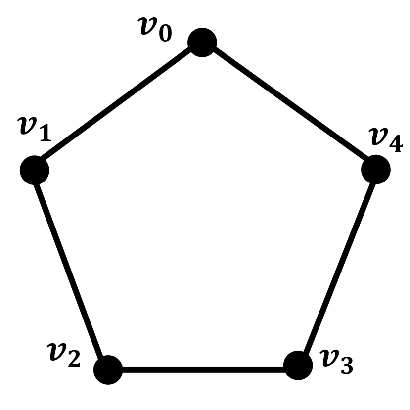
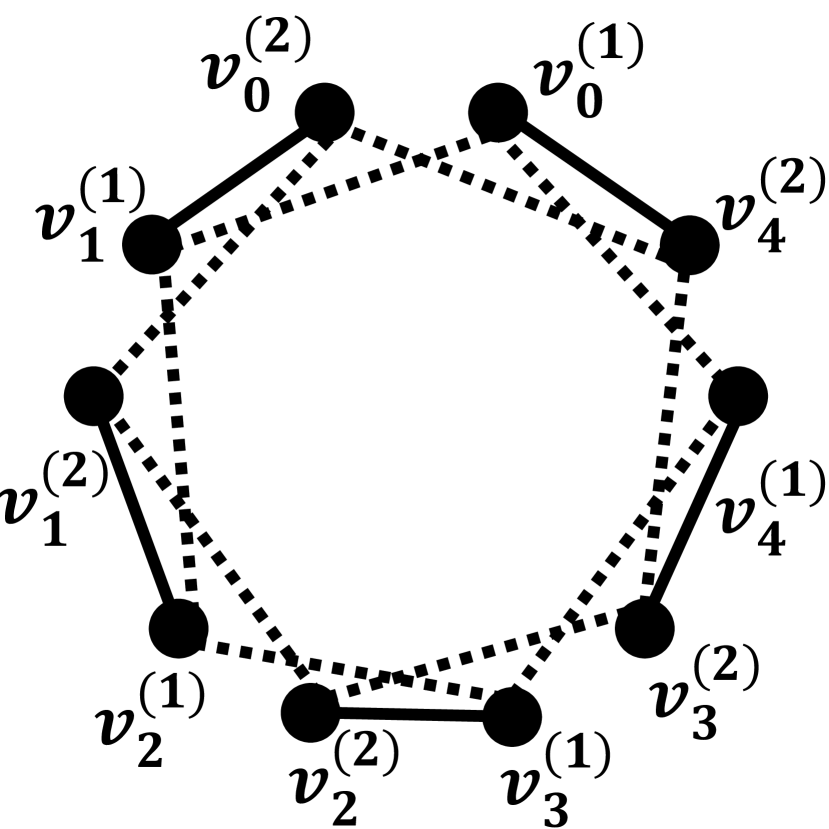
Figure 3: An example of (a) $C_{n},n=5$ and its $\epsilon$-graph (b) $C_{5,\epsilon}$. Note that the weight of each vertex in (a) is $1$, while the weight of each vertex in (b) is $\frac{1}{2}$.

The $\epsilon$-independence number $\alpha_{\epsilon}\left(C_{n,\epsilon},\bm{w}\right)$ is given by the convex combination of the independence numbers of two related graphs, $C_{n,\epsilon}^{\prime}$ and $C_{n,\epsilon}^{\prime\prime}$, with coefficients $\epsilon$ and $1-\epsilon$, respectively. The graph $C_{n,\epsilon}^{\prime}$ is a copy of $C_{n,\epsilon}$ with all the $\epsilon$-edges removed, resulting in $C_{n,\epsilon}^{\prime}$ being composed of $n$ disjoint cliques, each with a weight of $\frac{1}{2}$ on every vertex. It is straightforward to see that $\alpha(C_{n,\epsilon}^{\prime},\bm{w})=\frac{n}{2}$. The graph $C_{n,\epsilon}^{\prime\prime}$ is a copy of $C_{n,\epsilon}$ where all the $\epsilon$-edges are treated as normal edges. By Lemma 2, we have $\alpha(C_{n,\epsilon}^{\prime\prime},\bm{w})=\alpha(C_{n})=\frac{n-1}{2}$. Therefore, the $\epsilon$-independence number of $C_{n,\epsilon}$ is given by:

$$\alpha_{\epsilon}(C_{n,\epsilon},\bm{w})=\epsilon\cdot\frac{n}{2}+(1-\epsilon)\cdot\frac{n-1}{2}=\frac{n-1+\epsilon}{2}.$$ (22)

Thus for any odd-cycle $C_{n}$, the threshold $\epsilon$ is calculated as:

$$\begin{split}\alpha_{\epsilon}(C_{n,\epsilon})\leq\theta(C_{n})\Rightarrow\frac{n-1+\epsilon}{2}&\leq\frac{n\cos{\left(\frac{\pi}{n}\right)}}{1+\cos{\left(\frac{\pi}{n}\right)}}\\ \Rightarrow\epsilon&\leq 1-n+\frac{2n\cos{\left(\frac{\pi}{n}\right)}}{1+\cos{\left(\frac{\pi}{n}\right)}}\\ &=1+\frac{2n\left(\cos^{2}{\frac{\pi}{2n}}-\sin^{2}{\frac{\pi}{2n}}\right)-2n\cos^{2}{\frac{\pi}{2n}}}{2\cos^{2}{\frac{\pi}{2n}}}\\ &=1-n\tan^{2}{\frac{\pi}{2n}}\\ &\leq 1-n\cdot\left(\frac{\pi}{2n}\right)^{2}=1-\frac{\pi^{2}}{4n}\\ \end{split}$$ (23)

In other words, for any $\epsilon\in[0,1)$, we find that $\alpha_{\epsilon}(C_{n,\epsilon})\leq\theta(C_{n})$ when the length of the odd cycle satisfies $n\geq\lceil\frac{\pi^{2}}{4(1-\epsilon)}\rceil$.

∎

Appendix D Proof of Lemma. 1

Proof.

Suppose that $X^{*}$ and $Y^{*}$ are the maximizers corresponding to the solution of the SDP problem (8). We define the matrix $Z$ as:

$$Z:=\epsilon\cdot X^{*}+(1-\epsilon)\cdot Y^{*}.$$ (24)

This construction ensures that $Z\succeq 0$, $\operatorname{Tr}Z=1$, $Z_{ij}=0$ for all $(i,j)\in E$, and $Z_{ij}=\epsilon\cdot X^{*}_{ij}$ for all $(i,j)\in\widetilde{E}_{\epsilon}$. Additionally, we have $Z_{ii}=X^{*}_{ii}=Y^{*}_{ii}$ for all $i\in V$. Since $Z$ is positive semi-definite, its Cholesky decomposition yields $|V|$ vectors $v_{1}^{*},v_{2}^{*},\ldots,v_{|V|}^{*}$ such that $Z_{ij}={v_{i}^{*}}^{T}\cdot v_{j}^{*}$.

Next, we define the following unit vectors:

$$\begin{split}\widetilde{u_{i}}&:=\frac{v_{i}^{*}}{\|v_{i}^{*}\|}\quad\forall i\in V,\\ \widetilde{\psi}&:=\frac{\sum_{i=1}^{|V|}v_{i}^{*}}{\|\sum_{i=1}^{|V|}v_{i}^{*}\|}.\end{split}$$ (25)

The set of vectors $\{\widetilde{u_{i}}\},i\in V$ is an orthonormal representation of $G^{\prime}_{\epsilon}$, satisfying the strict orthogonality constraints arising from the normal edges. Moreover, this set also satisfies the $\epsilon$-orthogonality conditions for the $\epsilon$-edges. Specifically, for any $(i,j)\in\widetilde{E}_{\epsilon}$, we have:

$$\begin{split}\left|\widetilde{u_{i}}^{T}\cdot\widetilde{u_{j}}\right|=\frac{\left|{v_{i}^{*}}^{T}\cdot v_{j}^{*}\right|}{\|v_{i}^{*}\|\cdot\|v_{j}^{*}\|}=\frac{\left|Z_{ij}\right|}{\sqrt{Z_{ii}}\cdot\sqrt{Z_{jj}}}=\frac{\left|\epsilon\cdot X^{*}_{ij}\right|}{\sqrt{X^{*}_{ii}}\cdot\sqrt{X^{*}_{jj}}}\leq\epsilon.\end{split}$$ (26)

The last inequality holds because $X^{*}$ is also positive semi-definite and can be Cholesky decomposed into a set of vectors $\{x_{i}\},i\in V$, where $x_{i}^{T}\cdot x_{j}=X^{*}_{ij}$. Thus, $\frac{\left|X^{*}_{ij}\right|}{\sqrt{X^{*}_{ii}}\cdot\sqrt{X^{*}_{jj}}}=\frac{\left|x_{i}^{T}\cdot x_{j}\right|}{\|x_{i}\|\cdot\|x_{j}\|}=\left|\widetilde{x_{i}}^{T}\cdot\widetilde{x_{j}}\right|\leq 1$, where $\widetilde{x_{i}},\forall i\in V$ are normalized vectors from $x_{i}$.

Furthermore, since $\operatorname{Tr}Z=1$, we have $\sum_{i=1}^{|V|}\|v_{i}^{*}\|^{2}=1$. Given that

$$\theta^{\prime}_{\epsilon}(G_{\epsilon},\bm{w})=\epsilon\cdot(\sqrt{\bm{w}}^{T}X^{*}\sqrt{\bm{w}})+(1-\epsilon)\cdot(\sqrt{\bm{w}}^{T}Y^{*}\sqrt{\bm{w}})=\sqrt{\bm{w}}^{T}Z\sqrt{\bm{w}},$$ (27)

it follows that $\theta^{\prime}_{\epsilon}(G_{\epsilon},\bm{w})=\left(\sum_{i\in V}\sqrt{w_{i}}\cdot v_{i}^{*}\right)^{2}$

Thus, we have:

$$\begin{split}\sum_{i\in V}w_{i}\left(\widetilde{\psi}^{T}\cdot\widetilde{u_{i}}\right)^{2}&=\left(\sum_{i\in V}\|v_{i}^{*}\|^{2}\right)\left(\sum_{i\in V}w_{i}\left(\widetilde{\psi}^{T}\cdot\widetilde{u_{i}}\right)^{2}\right)\\ &\geq\left(\sum_{i\in V}\|v_{i}^{*}\|\cdot\sqrt{w_{i}}\left(\widetilde{\psi}^{T}\cdot\widetilde{u_{i}}\right)\right)^{2}\\ &=\left(\sum_{i\in V}\sqrt{w_{i}}\cdot\left(\widetilde{\psi}^{T}\cdot v_{i}^{*}\right)\right)^{2}\\ &=\left(\widetilde{\psi}^{T}\cdot\sum_{i\in V}\sqrt{w_{i}}\cdot v_{i}^{*}\right)^{2}\\ &=\left(\sum_{i\in V}\sqrt{w_{i}}\cdot v_{i}^{*}\right)^{2}=\theta^{\prime}_{\epsilon}(G_{\epsilon},\bm{w}).\end{split}$$ (28)

Thus, we have constructed a feasible, though not necessarily optimal, solution to the problem in Eq. (7) based on the solution to Eq. (8). This concludes the proof of the lemma. ∎

Appendix E $\epsilon$-Contextuality for a single Qubit system. – Proof of Theorem. 3

Proof.

Consider a set of $2n$ qubit states defined as $S:=\{|v_{k}^{0}\rangle,|v_{k}^{1}\rangle\}$ for $k=1,\ldots,n$, where

$$|v_{k}^{0}\rangle=\cos\left(\frac{k\pi}{2n}\right)|0\rangle+\sin\left(\frac{k\pi}{2n}\right)|1\rangle,\qquad|v_{k}^{1}\rangle=-\sin\left(\frac{k\pi}{2n}\right)|0\rangle+\cos\left(\frac{k\pi}{2n}\right)|1\rangle.$$ (29)

For all $k=1,\ldots,n$, we find that $|v_{k}^{0}\rangle$ is orthogonal to $|v_{k}^{1}\rangle$. Additionally, $|v_{k}^{0}\rangle$ is $\epsilon$-orthogonal to $|v_{k+1}^{1}\rangle$, and similarly $|v_{k}^{1}\rangle$ is $\epsilon$-orthogonal to $|v_{k+1}^{0}\rangle$ for all $k=1,\ldots,n-1$. Furthermore, $|v_{n}^{0}\rangle$ is $\epsilon$-orthogonal to $|v_{1}^{0}\rangle$, and $|v_{n}^{1}\rangle$ is $\epsilon$-orthogonal to $|v_{1}^{1}\rangle$. We calculate the corresponding parameter to be $\epsilon=|\sin\left(\frac{\pi}{2n}\right)|$. To establish $\epsilon$-edges, we implicitly assume $n\geq 2$, thus we have $\epsilon\leq\frac{1}{\sqrt{2}}$.

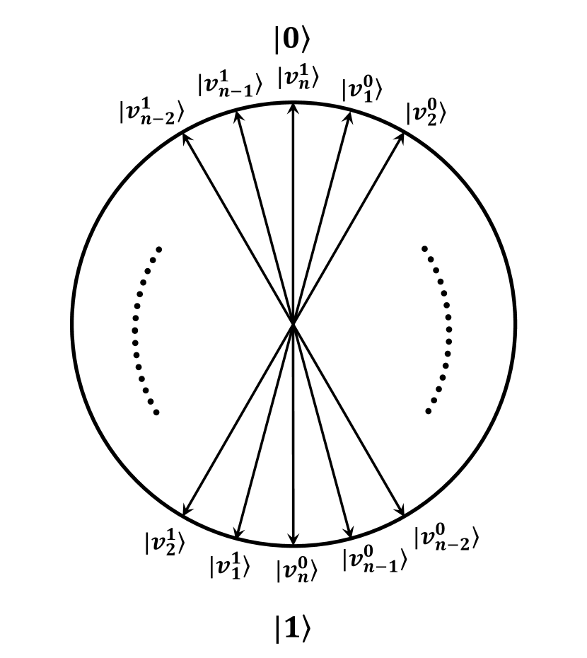
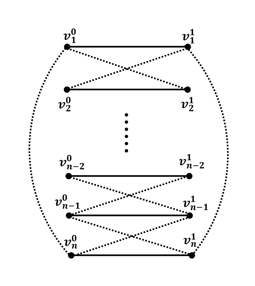
Figure 4: (a) The set of qubit states $S$ shown on the XZ plane of the Bloch sphere. (b) The $\epsilon$-orthogonality graph of $S$.

The $\epsilon$-orthogonality graph $G_{\epsilon}$ of these vectors is illustrated in Fig. 4, containing $n$ normal edges and $2n$ $\epsilon$-orthogonal edges. Each vertex has a weight of $1$. Since the vectors form $n$ complete bases in a Hilbert space of dimension $2$, we have:

$$\sum_{k=1}^{n}\left(|v_{k}^{0}\rangle\langle v_{k}^{0}|+|v_{k}^{1}\rangle\langle v_{k}^{1}|\right)=n\cdot\mathbb{I}_{2},$$ (30)

thus achieving $\theta_{\epsilon}(G_{\epsilon},\bm{w})=n$ with any qubit state for the particular projectors represented in $S$.

Recall that the independence number of the $\epsilon$-orthogonality graph $G_{\epsilon}$ can be computed from two related graphs: $G^{\prime}_{\epsilon}$ (including only the normal edges) and $G^{\prime\prime}_{\epsilon}$ (including all edges, treating the $\epsilon$-edges as normal). It’s straightforward to verify that $\alpha(G^{\prime}_{\epsilon})=n$ and $\alpha(G^{\prime\prime}_{\epsilon})=n-1$. Hence,

$$\alpha_{\epsilon}(G_{\epsilon})=\epsilon\cdot\alpha(G^{\prime}_{\epsilon})+(1-\epsilon)\cdot\alpha(G^{\prime\prime}_{\epsilon})=n-1+\epsilon.$$ (31)

Therefore, for any $\epsilon\in(0,\frac{1}{\sqrt{2}})$, there exists a finite set of $2n$ vectors as defined in $S$ with $n\geq\lceil\frac{\pi}{2\arcsin(\epsilon)}\rceil$ that exhibits the smooth version of the state-independent qubit contextuality argument. For large $n$, we see that a single qubit system is arbitrarily close to being contextual. ∎

Appendix F Using the derived quantum correlations in an SDI protocol

The quantum correlations certifying $\log_{2}d$ bits of randomness may be used in contextuality-based SDI randomness expansion protocols wherein the task is to expand a short fully random seed into a larger string of uniformly random bits. In these protocols, some initial randomness is required to perform the contextuality tests. To achieve a net positive generation rate, spot-checking protocols are commonly used. More precisely, an honest user runs the device for $N$ rounds, and each round is designated either as a test round with a low probability $\gamma\in(0,1)$, or as a randomness generation round with a high probability $(1-\gamma)$. In a test round, initial randomness is used to select an input (a context) to implement the contextuality test; and in a randomness generation round, a specific input setting $c^{*}$ (the context corresponding to a clique of size $d$ in the orthogonality graph $\mathcal{G}_{d}$) is chosen to generate raw randomness. At the end of the protocol, the quality of the raw randomness is assessed by analyzing the observed input-output data from the test rounds. Provided the protocol does not abort, the randomness accumulated during the randomness generation rounds is extracted by applying a suitable quantum-proof randomness extractor. We give a specific contextuality-based randomness expansion protocol below.

The uncertainty of a variable $A$ given side information $B$, evaluated for a joint state $\rho_{AB}$, is lower bounded by the conditional $\epsilon$-smooth min-entropy renner2004smooth , denoted as $H_{min}^{\epsilon}(A|B)_{\rho_{AB}}$. The Entropy Accumulation Theorem (EAT) arnon2018practical ; dupuis2020entropy is an information-theoretic tool that provides a way to lower bound the conditional $\epsilon$-smooth min-entropy accumulated over multiple rounds of a protocol, it allows the elevation of i.i.d. analyses to the non-i.i.d. setting. EAT achieves this by relating it to an average quantity that is straightforward to calculate, subject to some correction terms. For an $N$-round protocol such as shown below, under the condition that the protocol does not abort, the EAT states that

$$H_{min}^{\epsilon}(\bm{A}|\bm{X}E)\geq Nf_{\text{min}}(\omega)-O(\sqrt{N}),$$ (32)

where $\bm{A}$ represents the $N$-round outputs of the device, $\bm{X}$ denotes the $N$-round inputs, and $E$ is the adversary’s side information. The function $f_{\text{min}}(\omega)$, known as the min-tradeoff function, is a convex, differentiable function that maps the game score $\omega$ to $\mathbb{R}$ and lower bounds the worst-case von Neumann entropy:

$$f_{\text{min}}(\omega)\leq\inf H(A|XE),$$ (33)

where the right-hand side represents the single-round conditional von Neumann entropy compatible with the game score $\omega$.

To apply this theorem, it is necessary to confirm that the protocol setting meets the EAT requirements. In the following, we review the definitions of EAT channels as presented in arnon2018practical ; dupuis2020entropy , adapting them to the single-party setting required for our scenario, showing that the contextuality-based SDI randomness expansion protocol described in the main text meets the EAT requirements.

Protocol 1 Contextuality-based SDI QRE
Parameters:
$N$: number of rounds.
$\gamma\in(0,1)$: probability of a test round.
$c^{*}$: distinguished context for generation rounds.
$g$: a one-to-one function that maps outcomes of $c^{*}$ to $[d]$.
$\omega_{\text{exp}}$: expected score of $\mathcal{I}_{d}$ for an honest implementation.
$\delta$: width of the statistical confidence interval for game score.
$f_{\text{min}}$: min-trade off function.
$\epsilon_{\text{ext }}\in(0,1)$: extractor error.
$\epsilon_{s}\in(0,1)$: smoothing parameter.
$\epsilon_{\text{EAT}}\in(0,1)$: entropy accumulation error. (Choose to $\leq\epsilon_{\mathrm{ext}}+2\epsilon_{s}$)
$R_{\text{ext}}$: quantum-proof $(k,\epsilon_{\mathrm{ext}}+2\epsilon_{s})$-strong extractor.
$l_{\text{ext}}$: entropy loss induced by $R_{\text{ext}}$.
Protocol 1. For every round $i\in[N]$, choose $T_{i}\in\{0,1\}$ such that $T_{i}=1$ with probability $\gamma$. If $T_{i}=1$: Test round: Play a single round of $\mathcal{I}_{d}$ where the inputs $\{c\}$ (the contexts) are chosen uniformly at random using the initial private randomness. Record the input $c_{i}$ and the outputs $A_{i}$ of the sequential measurements in this context. Set the product of $A_{i}$ (outputs of the sequential measurements in this context) as the score $\omega_{i}$ of this round. Else $T_{i}=0$: Randomness generation round: Input $c^{*}$ into the device and record the outputs $A_{i}$ of the sequential measurements in this context. Set the score of this round as $\omega_{i}=0$. Record $g(A_{i})$ as the raw randomness $r_{i}$. 2. Compute the empirical score $\omega_{\text{obs}}:=\frac{\sum_{i=1}^{N}\omega_{i}}{\gamma\cdot N}.$ If $\omega_{\text{exp}}-\delta<\omega_{\text{obs}}<\omega_{\text{exp}}+\delta$: Extraction: Apply a strong quantum-proof randomness extractor $R_{\text{ext}}$ to the raw randomness string $\bm{r}$ to extract $Nf_{min}(\omega_{\text{exp}}-\delta)-l_{\text{ext}}$ bits of $\epsilon_{\text{ext}}+2\epsilon_{s}$-close to uniform random outputs. Else: Abort: Abort the protocol.

Definition 4.

(EAT Channels)
The EAT Channels $\mathcal{M}_{i}:R_{i-1}\rightarrow R_{i}A_{i}X_{i}W_{i}$ for $i\in[N]$ are completely positive trace-preserving (CPTP) maps such that

• $A_{i}X_{i}W_{i}$ are finite-dimensional classical random variables ($A_{i}$ is measurement outcome, $X_{i}$ is measurement input, $W_{i}$ is a random variable evaluating the game score of the contextuality test), $R_{i}$ are arbitrary quantum registers (holding information about the quantum state at the $i$-th round).

• For any input state $\rho_{R_{i-1}R^{\prime}}$ where $R^{\prime}$ is a register isomorphic to $R_{i-1}$, the classical value $W_{i}$ (the game score of the contextuality test at the $i$-th round) can be measured from the marginal $\rho_{A_{i}X_{i}}$ (the classical random variables at the round) of the output state $\rho_{R_{i}A_{i}X_{i}W_{i}R^{\prime}}=\left(\mathcal{M}_{i}\otimes\mathcal{I}_{R^{\prime}}\right)\left(\rho_{R_{i-1}R^{\prime}}\right)$ without changing the state.

• For any initial state $\rho_{R_{0}E}$, the final state $\rho_{\mathcal{A}^{N}\mathcal{X}^{N}\mathcal{W}^{N}E}=((\text{Tr}_{R_{N}}\circ\mathcal{M}_{N}\circ\cdots\mathcal{M}_{1})\otimes\mathcal{I}_{E})\rho_{R_{0}E}$ satisfies the Markov condition $\mathcal{A}^{i-1}\leftrightarrow\mathcal{X}^{i-1}E\leftrightarrow X_{i}$ for each $i\in[N]$. Here $\mathcal{A}^{i-1}=A_{1},A_{2},\ldots,A_{i-1}$ and similarly for the other random variables.

The channels $\mathcal{M}_{i}$ describe the actions of the device, including the choice of input settings $X_{i}$ determined by some initial private randomness, the device output $A_{i}$, and the observed game score $W_{i}$. The first condition in the EAT channels, compatible with the protocol structure, specifies that the inputs $X_{i}$, outputs $A_{i}$, and observed game score $W_{i}$ are classical, while the arbitrary quantum register $R_{i}$ represents the quantum state stored by the device after the $i$-th round. The last condition reflects the sequential nature of the protocol, where the Markov chain condition implies that the device input $X_{i}$ in the $i$-th round is conditionally independent of previous outputs $\mathcal{A}^{i-1}$. This holds because the device inputs are derived from an initial private random seed. Together, the second and last conditions characterize the adversary, who is permitted to hold a purification $E$ of the initial state of the device, and the joint state evolves with the sequential interaction through the application of the sequence of EAT channels.

Now, we recall the efficient derivation of min-tradeoff functions via the dual program of semidefinite programs, following the approach outlined in brown2019framework . In this work, we employ the min-entropy $H_{\text{min}}(A|XE)$ to bound the von Neumann entropy $H(A|XE)$ from below. The min-entropy is calculated through the guessing probability as follows:

$$H_{\text{min}}(A|XE):=-\log_{2}p_{\text{guess}}(A|XE).$$ (34)

The guessing probability represents the probability that an adversary, Eve, applies the best possible strategy using her system $E$ to guess the outcome $A$ of a measurement setting $X=x^{*}$. Suppose the state shared between the device and Eve is $\rho_{AE}$, the guessing probability is defined as

$$p_{\text{guess}}(A|X=x^{*},E):=\max_{\bm{p}}\sum_{a\in A}p(a,e=a|X=x^{*},E)=\max_{\{P_{e}\},\rho_{AE}}\sum_{a}\text{Tr}(P_{a}\otimes P_{e=a}\rho_{AE}),$$ (35)

where $\{P_{e}\}$ denotes the projective measurement on Eve’s system. In (semi-)device-independent scenarios, Eve can optimize her choice of measurement $\{P_{e}\}$ and the shared state $\rho_{AE}$ to maximize her guessing probability, covering all states and measurements that the device might use to achieve the best performance.

However, this optimization problem is challenging to efficiently solve because the objective function is nonlinear, and the optimal dimension of the quantum system is unknown, making the problem difficult to directly manage. We can relax this problem by employing the NPA (Navascués-Pironio-Acín) hierarchy navascues2007bounding ; navascues2008convergent , which replaces the tensor product structure of operators with commutation relations, translating the optimization problem into a SDP that can be efficiently computed. The NPA hierarchy introduces a sequence of correlation sets $\mathrm{Q}_{k}$, forming an outer approximation to the quantum correlation set, where $\mathrm{Q}_{1}\supsetneq\mathrm{Q}_{2}\supsetneq\mathrm{Q}_{3}\supsetneq\cdots\supsetneq\mathrm{Q}$. The solutions of these SDPs yield increasingly tighter upper bounds on the guessing probability.

The guessing probability must also be compatible with the observed game score $\omega$ for the contextuality test $\mathcal{I}_{d}$ (in our case, we use $\mathcal{I}_{3}$ presented in the main text). Thus, the relaxed guessing probability SDP can be expressed as

$$\begin{split}{p^{(k)}_{\text{guess}}}(\omega)=\max_{\bm{p}}&\quad\sum_{a\in A}p(a,e=a|X=x^{*},E)\\ \text{s.t.}&\quad\bm{p}\in\mathrm{Q}_{k},\\ &\quad\mathcal{I}(\bm{p})=\omega.\end{split}$$ (36)

This program can be expressed in a standard form:

$$\begin{split}{p^{(k)}_{\text{guess}}}(\omega)=\max_{P}&\quad\text{Tr}[GP]\\ \text{s.t.}&\quad\text{Tr}\left[S_{i}P\right]=s_{i}\quad\text{for all }i,\\ &\quad\text{Tr}\left[IP\right]=\omega,\\ &\quad P\geq 0,\end{split}$$ (37)

where each matrix $S_{i}$ and value $s_{i}$ corresponds to constraints on the NPA moment matrix $P$, such as commutation conditions for operators, the non-negative, normalization and no-signaling conditions for corresponding probabilities. The dual program is given by

$$\begin{split}{d^{(k)}_{\text{guess}}}(\omega)=\min_{\bm{\lambda}}&\quad\lambda_{0}\omega+\sum_{i}\lambda_{i}s_{i}\\ \text{s.t.}&\quad\lambda_{0}I+\sum_{i}\lambda_{i}S_{i}\geq G.\end{split}$$ (38)

According to the weak duality theorem, the solution to the dual program provides an upper bound on the solution of the primal SDP. The optimal solution for the Lagrange multipliers $\hat{\bm{\lambda}}$ at any fixed game score $\hat{\omega}$ forms an affine function $g_{\hat{\omega}}(\omega)$ that bounds the guessing probability curve ${p^{(k)}_{\text{guess}}}(\omega)$ from above for any $\omega$. Assuming strong duality holds, i.e., ${d^{(k)}_{\text{guess}}}(\hat{\omega})={p^{(k)}_{\text{guess}}}(\hat{\omega})$, then $g_{\hat{\omega}}(\omega)$ is tangent to the guessing probability curve ${p^{(k)}_{\text{guess}}}(\omega)$ at $\hat{\omega}$. This can be seen by observing that for any feasible solution $P$ of the primal program with game score $\omega$, we have:

$$\begin{split}0&\leq\text{Tr}\left[(\hat{\lambda}_{0}I+\sum_{i}\hat{\lambda}_{i}S_{i}-G)P\right]\\ &=\hat{\lambda}_{0}\text{Tr}[IP]+\sum_{i}\hat{\lambda}_{i}\text{Tr}[S_{i}P]-\text{Tr}[GP]\\ &=\hat{\lambda}_{0}\omega+\sum_{i}\hat{\lambda}_{i}s_{i}-\text{Tr}[GP]\\ &=g_{\hat{\omega}}(\omega)-\text{Tr}[GP].\end{split}$$ (39)

Thus, from the optimal solution of the dual program, we obtain a family of affine functions $\{g_{\hat{\omega}}(\omega)\}_{\hat{\omega}}$ that upper bound the guessing probability curve. The family of functions $\{f_{\hat{\omega}}(\omega):=-\log_{2}\left(g_{\hat{\omega}}(\omega)\right)\}_{\hat{\omega}}$ provides a lower bound on the min-entropy $H_{\text{min}}(A|X=x^{*},E)$ (and hence also on the von Neumann entropy $H(A|X=x^{*},E)$) for each game score $\omega$. Notably, since $g_{\hat{\omega}}(\omega)>0$ for all $\hat{\omega}$ as it upper bounds the guessing probability, the family of functions $\{f_{\hat{\omega}}(\omega)\}_{\hat{\omega}}$ are convex and differentiable, making them suitable candidates for the min-tradeoff function in the EAT theorem.

We numerically calculated the min-entropy curve with respect to the game score for $\mathcal{I}_{3}$ and generated a family of min-tradeoff functions accordingly, plotting them as below. Similar curves (and even possible enhancements achieved by computing the conditional von Neumann entropy) will be derived in forthcoming experimental implementations of contextuality-based SDI protocols.

Appendix G Attacks on SDI protocols for certain contextuality tests.

G.1 Attacks on state-independent contextuality-based protocols by a quantum adversary

State-independent contextuality (SI-C) as the name implies, allows for a contextuality test that does not depend on the choice of a particular quantum state. An SI-C can be written as a non-contextuality inequality for which the quantum value can be achieved by a set of observables $\{A_{i}\}_{i}$ acting on a fixed finite-dimensional Hilbert space with any state $\rho$ in the underlying space. Any KS set leads to a non-contextuality inequality of this type. Furthermore, it is also known that there are SI-C sets that do not correspond to a KS set yu2012state .

It is reasonably straightforward to observe that SI-C-based randomness certification protocols are not secure against a quantum adversary, even when the quantum values of these inequalities are observed. This is because the quantum value for a state-independent non-contextuality inequality in a Hilbert space of dimension $d$ can even be achieved by a maximally mixed state $\mathbb{I}/d$. When a quantum adversary shares the bipartite maximally entangled state $|\psi\rangle_{D,E}=\frac{1}{\sqrt{d}}\sum_{i=0}^{d-1}|i,i\rangle$ with the device operating the randomness certification protocol, the reduced system of the device can still observe the quantum value of the state-independent non-contextuality inequality. Furthermore, such an adversary is able to steer the state of the device depending on the publicly announced measurements made on the device, and thereby perfectly guess the corresponding measurement outcomes.

More specifically, in the contextuality test, a context $C$ includes $2\leq k\leq d$ mutually commuting observables $A_{1},\dots,A_{k}$ (with $A_{i}:=\mathbb{I}-2P_{i}$, where $P_{i}$ is a projector). By sharing a maximally entangled state, and the adversary measuring the same context with the device, the adversary’s outcome for each observable $A_{i}$ in this context is fully correlated with the outcome of the device:

$$\begin{split}\langle A_{i}\otimes A_{i}\rangle_{D,E}&=\langle\psi|_{D,E}(\mathbb{I}-2P_{i})\otimes(\mathbb{I}-2P_{i})|\psi\rangle_{D,E}\\ &=\langle\psi|_{D,E}\left(\mathbb{I}\otimes\mathbb{I}-2P_{i}\otimes\mathbb{I}-2\mathbb{I}\otimes P_{i}+4P_{i}\otimes P_{i}\right)|\psi\rangle_{D,E}\\ &=1+\langle\psi|_{D,E}\left(-2P_{i}\otimes(P_{i}+P_{i}^{\perp})-2(P_{i}+P_{i}^{\perp})\otimes P_{i}+4P_{i}\otimes P_{i}\right)|\psi\rangle_{D,E}\\ &=1-2\langle\psi|_{D,E}\left(P_{i}\otimes P_{i}^{\perp}+P_{i}^{\perp}\otimes P_{i}\right)|\psi\rangle_{D,E}=1.\end{split}$$ (40)

To circumvent this attack, one needs to use a private random source to choose the input settings, wherein the measurement settings used are not publicly known to the adversary. Alternatively, the honest user needs to perform several tests incorporating the full input-output statistics of the device.

G.2 Attacks on magic arrangement-based protocols by classical consistent adversaries

In this subsection, we present attacks on a specific class of protocols that use contextuality tests built upon magic arrangements. These are a well-known class of parity proofs that include the famous Peres-Mermin magic square and the Mermin star. Here, we consider attacks by classical adversaries (who share only classical correlations with the device implementing the protocol) who are nevertheless able to prepare general consistent (non-disturbing) behaviors for the device.

A class of quantum contextuality proofs is represented by the signed arrangements arkhipov2012extending $A=(V,E,l)$, where $V$ is the vertex set, $E$ is the hyperedge set, such that each vertex lies in exactly two hyperedges, and $l:E\to\{+1,-1\}$ is the labeling of each hyperedge with a sign of $+1$ or $-1$. The famous Peres-Mermin Magic Square contextuality proof can be understood as a signed arrangement shown in Fig. 7, where the labeling $l$ of the sign $+1$ is represented by the solid lines and the sign $-1$ is represented by the dashed lines in the figure. A classical realization of a signed arrangement $A=(V,E,l)$ is a map $f_{c}:V\to\{+1,-1\}$ such that $\prod_{v\in e}f_{c}(v)=l(e),\forall e\in E$. On the other hand, a quantum realization of a signed arrangement $A=(V,E,l)$ is a map $f_{q}$ that maps vertices to observables acting on a fixed finite-dimensional Hilbert space, such that the eigenvalues of each observable are $+1$ and $-1$, the observables commute if the corresponding vertices appear in a common hyperedge, and $\prod_{v\in e}f_{q}(v)=l(e)\mathbb{I}$ holds for any $e\in E$. The magic arrangements are those which are not classically realizable but are quantumly realizable.

In arkhipov2012extending , Arkhipov proved that the classical and quantum realizability of a signed arrangement $A=(V,E,l)$ depends on $l$ only via its parity, i.e., $\prod_{e\in E}l(e)$. Furthermore, it is necessary and sufficient for the parity of the magic arrangement to be $-1$. On the other hand, the intersection graph (we will formally define the intersection graph of a given arrangement later) of a magic arrangement is necessarily nonplanar. In other words, the intersection graph of a magic arrangement must contain the intersection graph of the magic square, i.e., the graph $K_{3,3}$, or the intersection graph of the magic pentagram, i.e., the graph $K_{5}$, as its topological minor. (We will formally define a graph topological minor later.) Thus, there is a systematic way to find the quantum realization of a magic arrangement directly from the quantum realization of the magic square or the magic pentagram.

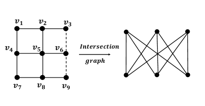
Figure 6: The Magic Square and its intersection graph $K_{3,3}.$ The sign of the dashed hyperedge is $-1$ and others are $+1$.

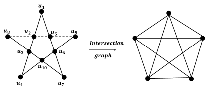
Figure 7: The Magic Pentagram and its intersection graph $K_{5}.$ The sign of the dashed hyperedge is $-1$ and others are $+1$.

In this section, we are interested in attacks by a no-signaling adversary who can prepare arbitrary no-signaling behaviors for the device. In the contextuality test for a single system, the no-signaling conditions are reduced to the non-disturbance conditions, which indicate that the probability of the outcome of each vertex is independent of which hyperedge it belongs to. Denote $\bm{v}_{e}$ as a string of outcomes of vertices in hyperedge $e$, and denote $n_{e}$ as the number of vertices in hyperedge $e$, so $\bm{v}_{e}\in\{+1,-1\}^{n_{e}}$. Denote $[\bm{v}_{e}]_{v}$ as the value of vertex $v$ for a given output string $\bm{v}_{e}$, and $\overline{[\bm{v}_{e}]}_{v}$ as the outcome string without the value of $v$. The no-signaling realization of a signed arrangement $A=(V,E,l)$ is a behavior $\{p(\bm{v}_{e}|e)\}$ such that

$$\sum_{\bm{v}_{e}:\prod_{v\in e}[\bm{v}_{e}]_{v}=l(e)}p(\bm{v}_{e}|e)=1,\forall e\in E.$$ (41)

In addition, the non-disturbance condition holds:

$$p(v|e)=\sum_{\overline{[\bm{v}_{e}]}_{v}}p(\bm{v}_{e}|e)=\sum_{\overline{[\bm{v}_{e^{\prime}}]}_{v}}p(\bm{v}_{e^{\prime}}|e^{\prime})=p(v|e^{\prime}),\forall v\in V,\forall e,e^{\prime}\in E\text{ that }v\in e,e^{\prime}.$$ (42)

Proposition 1.

The no-signaling realizability of a signed arrangement $A=(V,E,l)$ depends on $l$ only via its parity $\prod_{e\in E}l(e)$.

Arkhipov proved this proposition for classical and quantum realizations in arkhipov2012extending . Here, we provide a proof for the no-signaling realization, motivated by his result.

Proof.

To prove this proposition, we show that the no-signaling realizability of $A=(V,E,l)$ is the same as that of $A^{\prime}=(V,E,l^{\prime})$ when the parities of their labelling functions are the same, i.e., $\prod_{e\in E}l(e)=\prod_{e\in E}l^{\prime}(e)$. Specifically, suppose that $A$ has a no-signaling realization $\{p(\bm{v}_{e}|e)\}$. We will construct a corresponding no-signaling realization $\{p^{\prime}(\bm{v}_{e}|e)\}$ for $A^{\prime}$.

First, suppose that $l^{\prime}$ is obtained by flipping the signs $l$ assigns to two hyperedges $a$ and $b$ that contain a common vertex $v^{*}$. We can construct the no-signaling realization $\{p^{\prime}(\bm{v}_{e}|e)\}$ for $A^{\prime}$ as follows:

$$p^{\prime}(\overline{[\bm{v}_{e}]}_{v^{*}},v^{*}|e):=\begin{cases}p(\overline{[\bm{v}_{e}]}_{v^{*}},-v^{*}|e),&\text{when }e=a\text{ or }b;\\ p(\overline{[\bm{v}_{e}]}_{v^{*}},v^{*}|e),&\text{otherwise.}\end{cases}$$ (43)

where $-v^{*}$ denotes the negation of the value of $v^{*}$. In this way, we have:

$$\sum_{\bm{v}_{e}:\prod_{v\in e}[\bm{v}_{e}]_{v}=l^{\prime}(e)}p^{\prime}(\bm{v}_{e}|e)=\sum_{\bm{v}_{e}:\prod_{v\in e}[\bm{v}_{e}]_{v}=l(e)}p(\bm{v}_{e}|e),\forall e\in E.$$ (44)

Note that for an arrangement, each vertex belongs to exactly two hyperedges. Thus, the non-disturbance conditions hold for the no-signaling realization $\{p^{\prime}(\bm{v}_{e}|e)\}$ by the above construction. Specifically, we have:

$$\begin{split}p^{\prime}(v^{*}|e)&=p(-v^{*}|e),\quad\text{where }e=a\text{ or }b;\\ p^{\prime}(v|e)&=p(v|e),\quad\forall v\in V\setminus v^{*},\forall e\ni v.\end{split}$$ (45)

Now, suppose that $l^{\prime}$ is obtained by flipping the signs $l$ assigns to two hyperedges $a$ and $b$ that do not share any common vertex. Ignoring the labelling function $l$, an arrangement is simply a finite, connected hypergraph. Therefore, there must be a path $e_{0},e_{1},\ldots,e_{n}$ of distinct edges starting at $e_{0}=a$ and ending at $e_{n}=b$, such that any pair of adjacent hyperedges $e_{i},e_{i+1}$ ($i\in\{0,\ldots,n-1\}$) intersects at a vertex $v_{i}$. For each $v_{i}$, updating the no-signaling realization $\{p(\bm{v}_{e}|e)\}$ as in Eq. (43) results in the desired no-signaling realization $\{p^{\prime}(\bm{v}_{e}|e)\}$ for $A^{\prime}$. By repeatedly updating the no-signaling realizations, one can go from one labelling to any other one of equal parity.

∎

Proposition 2.

Suppose that an intersection graph $H$ is a topological minor of an intersection graph $G$, and the parity of their vertex labelings are the same, If the arrangement of $H$ has a no-signaling realization then the arrangement of $G$ also has a no-signaling realization.

Proof.

We prove that from the no-signaling realization $\{p(\bm{v}_{e}|e)\}$ of the arrangement corresponding to $H$, we can construct a no-signaling realization of the arrangement corresponding to $G$. To do this, we first need to formally define the intersection graph of a given arrangement and the concept of a graph topological minor.

Definition 5.

arkhipov2012extending The intersection graph of a signed arrangement $A=(V,E,l)$ is a graph $G=(V^{\prime},E^{\prime})$, where $V^{\prime}=E$, and there is an edge between $e_{1},e_{2}\in V^{\prime}$ for each vertex in $V$ that is in the intersection $e_{1}\cap e_{2}$. The labeling $l$ of hyperedges in $A$ is automatically translated into the labeling of vertices in $G$, which we denote by $l^{\prime}$.

Suppose that the vertex labeling of $H$ is $l^{\prime}$. For any vertex $v$ of $H$, assign the same sign $l^{\prime}(v)$ to the corresponding vertex $\phi(v)$ in $G$, and assign the label $+1$ to the other vertices in $G$.

Definition 6.

arkhipov2012extending A graph $H$ is a topological minor of $G$ if there exists an embedding of $H$ in $G$ consisting of an injective map $\phi$ that takes each vertex $v$ of $H$ to a vertex $\phi(v)$ of $G$, and a map from each edge $(u,v)$ of $H$ to a simple path from $\phi(u)$ to $\phi(v)$ in $G$, such that these paths are disjoint except at their endpoints.

Now, we construct the no-signaling realization of $G$ using the above inclusion map as follows. For each edge $e$ of $H$, the outcome of each edge (i.e., the outcomes of the corresponding vertices in the arrangement) is correlated with the outcome of $e$ in $H$, consistent with the probabilities given in the behavior $\{p(\bm{v}_{e}|e)\}$. The remaining edges in $G$ are assigned value $+1$. The resulting box $\{p^{\prime}(\bm{v}_{e}|e)\}$ is a valid no-signaling realization of the arrangement of $G$. Specifically, for each vertex $\phi(v)$ of $G$, the outcomes of the edges connected to it are either correlated with the outcomes of edges connected to $v$ in $H$ or are $+1$. The labelling of $\phi(v)$ is equal to the labelling of $v$ in $H$. Thus, the product of the outcomes of edges connected to $\phi(v)$ must equal its parity. For the other vertices of $G$, their parity is $+1$, and the edges connected to them always yield $+1$. On the other hand, the marginal probability of the outcome of each edge of $G$ is well-defined because it is either always $+1$ or correlated with the outcome of the edge of $H$, consistent with $\{p(\bm{v}_{e}|e)\}$. Thus, the non-disturbance conditions hold. Combined with Proposition 1, we obtain the claimed result. ∎

Proposition 3.

Magic arrangement-based randomness generation protocols are not secure against classical adversaries who can prevent consistent behaviors for the device.

Proof.

To prove this, we show that for both the magic square and the magic pentagram, for any hyperedge $e^{*}\in E$, there always exists a no-signaling realization that assigns deterministic outcomes to the vertices belonging to $e^{*}$. Specifically, for any hyperedge $e^{*}\in E$, there exists a no-signaling realization $\{p(\bm{v}_{e}|e)\}$ such that $p(\bm{v}_{e^{*}}|e^{*})\in\{0,1\}$. Thus, a no-signaling adversary capable of preparing arbitrary no-signaling boxes for the device can perfectly predict the outcome of $e^{*}$. Furthermore, since the intersection graph of any magic arrangement always contains $K_{3,3}$ or $K_{5}$ as a topological minor, and due to the no-signaling realizations constructed in Proposition 1 and Proposition 2, this no-signaling attack holds for any magic arrangement.

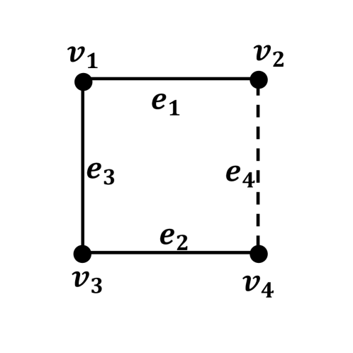
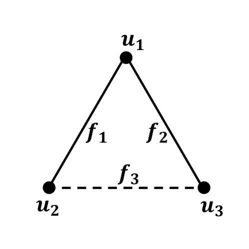
Figure 8: Two signed arrangements with parity $-1$. (a) $K_{2,2}$ contains four vertices and four hyperedges, with the sign of $e_{4}$ being $-1$ and the others being $+1$. (b) $K_{3}$ contains three vertices and three hyperedges, with the sign of $f_{3}$ being $-1$ and the others being $+1$.

Let’s consider two signed arrangements with parity $-1$, as shown in Fig. 8. Fig. 8 represents $K_{2,2}$, which contains four vertices $v_{1},\ldots,v_{4}$ and four hyperedges $e_{1},\ldots,e_{4}$. Fig. 8 represents $K_{3}$, which contains three vertices $u_{1},u_{2},u_{3}$ and three hyperedges $f_{1},f_{2},f_{3}$. The labels of the hyperedges $e_{4}$ and $f_{3}$ are $-1$, while the others are $+1$. The no-signaling realization for Fig. 8 is $\{p_{K_{2,2}}(\bm{v}_{e}|e)\}$, which satisfies the following identities:

$$\begin{split}p_{K_{2,2}}(v_{1}=v_{2}=+1|e_{1})=p_{K_{2,2}}(v_{1}=v_{2}=-1|e_{1})=\frac{1}{2},\;p_{K_{2,2}}(v_{1}=+1,v_{2}=-1|e_{1})=p_{K_{2,2}}(v_{1}=-1,v_{2}=+1|e_{1})=0;\\ p_{K_{2,2}}(v_{3}=v_{4}=+1|e_{2})=p_{K_{2,2}}(v_{3}=v_{4}=-1|e_{2})=\frac{1}{2},\;p_{K_{2,2}}(v_{3}=+1,v_{4}=-1|e_{2})=p_{K_{2,2}}(v_{3}=-1,v_{4}=+1|e_{2})=0;\\ p_{K_{2,2}}(v_{1}=v_{3}=+1|e_{3})=p_{K_{2,2}}(v_{1}=v_{3}=-1|e_{3})=\frac{1}{2},\;p_{K_{2,2}}(v_{1}=+1,v_{3}=-1|e_{3})=p_{K_{2,2}}(v_{1}=-1,v_{3}=+1|e_{3})=0;\\ p_{K_{2,2}}(v_{2}=+1,v_{4}=-1|e_{4})=p_{K_{2,2}}(v_{2}=-1,v_{4}=+1|e_{4})=\frac{1}{2},\;p_{K_{2,2}}(v_{2}=v_{4}=+1|e_{4})=p_{K_{2,2}}(v_{2}=v_{4}=-1|e_{4})=0.\end{split}$$ (46)

The marginal probability of the outcome for each vertex is $\frac{1}{2}$, i.e., $p_{K_{2,2}}(v_{i}|e)=\frac{1}{2}$ for all $v_{i}$ and for all $e\ni v_{i}$, ensuring the non-disturbance conditions hold. It is also easy to verify that for each edge, the product of the outcomes of the vertices belonging to that edge is always equal to the labeling of that edge. Similarly, a valid no-signaling realization for Fig. 8 is $\{p_{K_{3}}(\bm{v}_{e}|e)\}$, which satisfies the following identities:

$$\begin{split}p_{K_{3}}(u_{1}=u_{2}=+1|f_{1})=p_{K_{3}}(u_{1}=u_{2}=-1|f_{1})=\frac{1}{2},\;p_{K_{3}}(u_{1}=+1,u_{2}=-1|f_{1})=p_{K_{3}}(u_{1}=-1,u_{2}=+1|f_{1})=0;\\ p_{K_{3}}(u_{1}=u_{3}=+1|f_{2})=p_{K_{3}}(u_{1}=u_{3}=-1|f_{2})=\frac{1}{2},\;p_{K_{3}}(u_{1}=+1,u_{3}=-1|f_{2})=p_{K_{3}}(u_{1}=-1,u_{3}=+1|f_{2})=0;\\ p_{K_{3}}(u_{2}=+1,u_{3}=-1|f_{3})=p_{K_{3}}(u_{2}=-1,u_{3}=+1|f_{3})=\frac{1}{2},\;p_{K_{3}}(u_{2}=u_{3}=+1|f_{3})=p_{K_{3}}(u_{2}=u_{3}=-1|f_{3})=0.\end{split}$$ (47)

Both $K_{2,2}$ and $K_{3}$ are isomorphic to their respective intersection graphs. It’s straightforward to see that Fig. 8 is a topological minor of the graph $K_{3,3}$, the intersection graph of the magic square. For any hyperedge $c^{*}$ of the magic square, there exists an injective map $\phi$ from $K_{2,2}$ to $K_{3,3}$, as defined in Definition 6, such that the preimage of $c^{*}$ is empty. Due to the construction presented in Proposition 2, there exists a no-signaling realization of the magic square such that the output of $c^{*}$ is deterministic.

A similar phenomenon occurs for the magic pentagram. This is because Fig. 8 is a topological minor of the graph $K_{5}$, the intersection graph of the magic pentagram. For any hyperedge $c^{*}$ of the magic pentagram, there exists an injective map $\phi$ from $K_{3}$ to $K_{5}$, as defined in Definition 6, such that the preimage of $c^{*}$ is empty. ∎

References

- (1) A. K. Ekert. Quantum cryptography based on Bell’s theorem. Physical Review Letters 67(6): 661 (1991).
- (2) M. Herrero-Collantes and J. C. Garcia-Escartin. Quantum random number generators. Reviews of Modern Physics 89(1): 015004 (2017).
- (3) S. Pironio, A. Acín, S. Massar, A. Boyer de la Giroday, D. N. Matsukevich, P. Maunz, S. Olmschenk, D. Hayes, L. Luo, T. A. Manning, and C. Monroe. Random numbers certified by Bell’s theorem. Nature 464(7291): 1021 – 1024 (2010).
- (4) S. Pironio and S. Massar. Security of practical private randomness generation. Physical Review A 87(1): 012336 (2013).
- (5) P. J. Brown, S. Ragy, and R. Colbeck. A framework for quantum-secure device-independent randomness expansion. IEEE Transactions on Information Theory 66(5): 2964–2987 (2019).
- (6) W.-Z. Liu, M.-H. Li, S. Ragy, S.-R. Zhao, B. Bai, Y. Liu, P. J. Brown, J. Zhang, R. Colbeck, J. Fan, et al. Device-independent randomness expansion against quantum side information. Nature Physics 17(4): 448–451 (2021).
- (7) R. Colbeck and R. Renner. Free randomness can be amplified. Nature Physics 8(6): 450 – 453 (2012).
- (8) R. Gallego, L. Masanes, G. De La Torre, C. Dhara, L. Aolita, and A. Acín. Full randomness from arbitrarily deterministic events. Nature Communications 4(1): 1 – 7 (2013).
- (9) R. Ramanathan, F. G. S. L. Brandão, K. Horodecki, M. Horodecki, P. Horodecki, and H. Wojewódka. Randomness Amplification under Minimal Fundamental Assumptions on the Devices. Physical Review Letters 117(23): 230501 (2016).
- (10) F. G. S. L. Brandão, R. Ramanathan, A. Grudka, K. Horodecki, M. Horodecki, P. Horodecki, T. Szarek, and H. Wojewódka. Realistic noise-tolerant randomness amplification using finite number of devices. Nature Communications 7(1): 1 – 6 (2016).
- (11) R. Ramanathan, M. Horodecki, H. Anwer, S. Pironio, K. Horodecki, M. Grünfeld, S. Muhammad, M. Bourennane, and P. Horodecki. Practical no-signaling proof randomness amplification using Hardy paradoxes and its experimental implementation. arXiv: 1810.11648 (2018).
- (12) M. Kessler and R. Arnon-Friedman. Device-Independent Randomness Amplification and Privatization. IEEE Journal on Selected Areas in Information Theory 1(2): 568 – 584 (2020).
- (13) S. Zhao, R. Ramanathan, Y. Liu, and P. Horodecki. Tilted Hardy paradoxes for device-independent randomness extraction. Quantum 7, 1114 (2023).
- (14) R. Ramanathan, M. Banacki, and P. Horodecki. No-signaling-proof randomness extraction from public weak sources. arXiv: 2108.08819 (2021).
- (15) R. Ramanathan. Finite device-independent extraction of a block min-entropy source against quantum adversaries. arXiv preprint arXiv:2304.09643 (2023).
- (16) A. A. Abbott, C. S. Calude, J. Conder, and K. Svozil. Strong Kochen-Specker theorem and incomputability of quantum randomness. Physical Review A 86(6): 062109 (2012).
- (17) A. A. Abbott, C. S. Calude, and K. Svozil. Value-indefinite observables are almost everywhere. Physical Review A 89(3): 032109 (2014).
- (18) A. A. Abbott, C. S. Calude, and K. Svozil. A variant of the Kochen-Specker theorem localising value indefiniteness. Journal of Mathematical Physics 56(10) (2015).
- (19) J. Singh, K. Bharti, and A. Arvind. Quantum key distribution protocol based on contextuality monogamy. Physical Review A 95(6): 062333 (2017).
- (20) J. Singh, C. Foreman, K. Bharti, and A. Cabello. Local contextuality-based self-tests are sufficient for randomness expansion secure against quantum adversaries. arXiv preprint arXiv:2409.20082 (2024).
- (21) M. Um, X. Zhang, J. Zhang, Y. Wang, S. Yangchao, D.-L. Deng, L.-M. Duan, and K. Kim. Experimental certification of random numbers via quantum contextuality. Scientific Reports 3(1): 1627 (2013).
- (22) M. Um, Q. Zhao, J. Zhang, P. Wang, Y. Wang, M. Qiao, H. Zhou, X. Ma, and K. Kim. Randomness expansion secured by quantum contextuality. Physical Review Applied 13(3): 034077 (2020).
- (23) R. Ramanathan, M. Rosicka, K. Horodecki, S. Pironio, M. Horodecki, and P. Horodecki. Gadget structures in proofs of the Kochen-Specker theorem. Quantum, 4: 308, (2020).
- (24) Y. Liu, R. Ramanathan, K. Horodecki, M. Rosicka, and P. Horodecki. Optimal measurement structures for contextuality applications. npj Quantum Information, 9(1):63 (2023).
- (25) A. Acín, S. Pironio, T. Vértesi, and P. Wittek. Optimal randomness certification from one entangled bit. Physical Review A 93(4): 040102 (2016).
- (26) J. J. Borkała, C. Jebarathinam, S. Sarkar, and R. Augusiak. Device-independent certification of maximal randomness from pure entangled two-qutrit states using non-projective measurements. Entropy 24(3): 350 (2022).
- (27) S. Sarkar, J. J. Borkała, C. Jebarathinam, O. Makuta, D. Saha, and R. Augusiak. Self-testing of any pure entangled state with the minimal number of measurements and optimal randomness certification in a one-sided device-independent scenario. Physical Review Applied 19(3): 034038 (2023).
- (28) M. Farkas, J. Volčič, S. A. L. Storgaard, R. Chen, and L. Mančinska. Maximal device-independent randomness in every dimension. arXiv preprint arXiv:2409.18916 (2024).
- (29) A. Winter. What does an experimental test of quantum contextuality prove or disprove? Journal of Physics A: Mathematical and Theoretical 47(42): 424031 (2014).
- (30) R. Arnon-Friedman, F. Dupuis, O. Fawzi, R. Renner, and T. Vidick. Practical device-independent quantum cryptography via entropy accumulation. Nature Communications 9(1): 459 (2018).
- (31) F. Dupuis, O. Fawzi, and R. Renner. Entropy accumulation. Communications in Mathematical Physics 379(3): 867–913 (2020).
- (32) D. A. Meyer. Finite precision measurement nullifies the Kochen-Specker theorem. Physical Review Letters 83(19): 3751 (1999).
- (33) A. Kent. Noncontextual hidden variables and physical measurements. Physical Review Letters 83(19): 3755 (1999).
- (34) R. Clifton and A. Kent. Simulating quantum mechanics by non-contextual hidden variables. Proceedings of the Royal Society of London. Series A: Mathematical, Physical and Engineering Sciences 456(2001): 2101–2114 (2000).
- (35) J. S. Bell. On the problem of hidden variables in quantum mechanics. Reviews of Modern Physics 38(3): 447 (1966).
- (36) S. Kochen and E. P. Specker. The problem of hidden variables in quantum mechanics. Ernst Specker Selecta: 235–263 (1990).
- (37) A. Cabello. Kochen-Specker theorem for a single qubit using positive operator-valued measures. Physical Review Letters 90(19): 190401 (2003).
- (38) A. Grudka and P. Kurzyński. Is there contextuality for a single qubit? Physical Review Letters 100(16): 160401 (2008).
- (39) A. Cabello, M. G. Parker, G. Scarpa, and S. Severini. Exclusivity structures and graph representatives of local complementation orbits. Journal of Mathematical Physics 54(7) (2013).
- (40) A. Cabello, S. Severini, and A. Winter. Graph-theoretic approach to quantum correlations. Physical Review Letters 112(4): 040401 (2014).
- (41) P. Milgrom and I. Segal. Envelope theorems for arbitrary choice sets. Econometrica 70(2): 583–601 (2002).
- (42) L. Lovász. On the Shannon capacity of a graph. IEEE Transactions on Information Theory 25(1): 1–7 (1979).
- (43) R. Renner and S. Wolf. Smooth Rényi entropy and applications. In International Symposium on Information Theory, 2004. ISIT 2004. Proceedings., p. 233. IEEE (2004).
- (44) M. Navascués, S. Pironio, and A. Acín. Bounding the set of quantum correlations. Physical Review Letters 98(1): 010401 (2007).
- (45) M. Navascués, S. Pironio, and A. Acín. A convergent hierarchy of semidefinite programs characterizing the set of quantum correlations. New Journal of Physics 10(7): 073013 (2008).
- (46) S. Yu and C. H. Oh. State-independent proof of Kochen-Specker theorem with 13 rays. Physical Review Letters 108(3): 030402 (2012).
- (47) A. Arkhipov. Extending and characterizing quantum magic games. arXiv preprint arXiv:1209.3819 (2012).