A canonical foliation on null infinity in perturbations of Kerr

Abstract

Kerr stability for small angular momentum has been proved by Klainerman-Szeftel, Giorgi-Klainerman-Szeftel and Shen in the series of works [29, 30, 31, 19, 40]. Some of the most basic conclusions of the result, concerning various physical quantities on the future null infinity $\mathscr{I}^{+}$ are derived in Section 3.8 of [31]. Further important conclusions were later derived in [1] and [8]. In this paper, based on the existence and uniqueness results for GCM spheres of [29, 30], we establish the existence of a canonical foliation on $\mathscr{I}^{+}$ for which the null energy, linear momentum, center of mass and angular momentum are well defined and satisfy the expected physical laws of gravitational radiation. The rigid character of this foliation eliminates the usual ambiguities related to these quantities in the physics literature. We also show that under the initial assumption of [31, 19], the center of mass of the black hole has a large deformation (recoil) after the perturbation.

Dedicated to Demetrios Christodoulou and Roger Penrose.

Keywords

Kerr stability, future null infinity, outgoing PG foliation, intrinsic GCM spheres, geodesic foliation, LGCM foliation, regularity up to null infinity, supertranslation ambiguity, Bondi mass loss, center of mass, angular momentum, gravitational wave recoil, black hole kick.

Contents

1. 1 Introduction
   1. 1.1 Kerr stability for small angular momentum
   2. 1.2 General covariant modulated (GCM) procedure
      1. 1.2.1 Null horizontal structures
      2. 1.2.2 Deformations of spheres and frame transformations
      3. 1.2.3 Basis of $\ell=1$ modes
      4. 1.2.4 GCM spheres and incoming geodesic foliation
   3. 1.3 First version of main results
      1. 1.3.1 Regularity of conformal metric up to $\mathscr{I}^{+}$
      2. 1.3.2 Limiting GCM (LGCM) foliation on $\mathscr{I}^{+}$
      3. 1.3.3 Absence of supertranslation and spatial translation
      4. 1.3.4 Physical laws on $\mathscr{I}^{+}$
      5. 1.3.5 Gravitational wave recoil
   4. 1.4 Structure of the paper
   5. 1.5 Acknowledgements
2. 2 Preliminaries
   1. 2.1 Null horizontal structures
   2. 2.2 Hodge systems
   3. 2.3 Outgoing PG structures
   4. 2.4 $\operatorname{KSAF^{+}}$ spacetime $(\mathcal{M},{\bf g})$
   5. 2.5 Schematic notation $\Gamma_{g}$ and $\Gamma_{b}$
   6. 2.6 Commutation formulae
   7. 2.7 Main equations for an outgoing PG structure
      1. 2.7.1 Main equations in complex notations
      2. 2.7.2 Linearized equations in complex notation
      3. 2.7.3 Transport equations for metric components
   8. 2.8 Null frame transformation
3. 3 Asymptotic behavior near future null infinity
   1. 3.1 Limits of geometric quantities
   2. 3.2 Limits of pointwise physical quantities
   3. 3.3 Taylor expansions near future null infinity
4. 4 Conformal quantities and regularity up to $\mathscr{I}^{+}$
   1. 4.1 Asymptotic behavior of metric components
   2. 4.2 Conformal compactification of $\mathcal{M}$
   3. 4.3 Regularity up to $\mathscr{I}^{+}$ in perturbations of Kerr
   4. 4.4 Regularity up to $\mathscr{I}^{+}$ for other spacetimes
5. 5 Existence of Limiting GCM (LGCM) foliation
   1. 5.1 Definition of Limiting GCM (LGCM) foliation
   2. 5.2 Intrinsic GCM spheres
   3. 5.3 Construction of Limiting GCM (LGCM) foliation
      1. 5.3.1 Construction of a sequence of incoming null cones
      2. 5.3.2 Estimates for the sequence of incoming null cones
      3. 5.3.3 Limiting process
   4. 5.4 Proof of Theorem 5.4
6. 6 Absence of supertranslation ambiguity and spatial translation freedom
7. 7 Physical quantities in the LGCM foliation
8. 8 Displacement of the center of mass in Kerr stability
   1. 8.1 Total flux of physical quantities
   2. 8.2 Gravitational wave recoil
9. A Asymptotic behavior of geometric quantities
   1. A.1 Main equations in general setting
   2. A.2 Proof of Theorem 3.9
10. B Notations and conventions

1 Introduction

The definitions of conserved quantities such as mass and angular momentum have been among the most controversial problems of general relativity, see [45, 24] for a more recent survey. Among these challenges, a major issue is the definition of an angular momentum for a distant observer at null infinity. The difficulty, rooted in the equivalence principle, is due to the absence of a local energy-momentum density for the gravitational field. Indeed, the symmetric energy-momentum of matter $T_{\mu\nu}$, verifying the local conservation laws ${\bf D}^{\nu}T_{\mu\nu}=0$, is obtained by taking the variation of the corresponding action integral $\int L_{M}\operatorname{dvol}_{\bf g}$ of matter. The conserved quantities can then be defined, in causal regions of a spacetime that admits a Killing vectorfield $X$, by integrating the divergence ${\bf D}^{\mu}P_{\mu}=0$, with $P_{\mu}=T_{\mu\nu}X^{\nu}$. In the particular case of a Kerr spacetime this leads to a well defined of local versions of energy and angular momentum for the corresponding matter field. The same procedure applied to the gravitational action $\int\mathbf{R}\operatorname{dvol}_{\bf g}$ leads, however, to the Einstein tensor $\mathbf{R}_{\mu\nu}-\frac{1}{2}{\bf g}_{\mu\nu}\mathbf{R}$, that is, the left hand side of the actual Einstein field equations.

In view of these difficulties, mathematical physicists have given up on a local notion of energy-momentum for general gravitational fields and restrict instead to asymptotically flat metrics where the null energy and angular momentum can be defined as limits of appropriate quantities at spacelike and null infinity. The definitions of the correct limits (ADM quantities) at $i_{0}$ have been well understood since the seminal [2] paper. The first definitions at null infinity, due to [4, 38, 35], have generated much more controversy due to the ad hoc, non dynamical, definition of null infinity. Indeed, to be able to define the Bondi mass and angular momentum, one has to make specific asymptotic assumptions about the behavior of the metric at null infinity, which can only be verified by a rigorous, evolutionary, mathematical construction from prescribed initial data. The first such result, for general perturbations of Minkowski spacetime, is due to [13]. In the context of general perturbations of a slowly rotating Kerr spacetime, this was first achieved in the sequence of papers [31, 19, 29, 30, 40].

Prior to such a construction, the definition of the main physical quantities at null infinity, especially the angular momentum remained subject to possible ambiguities due to the presence of supertranslations, an infinite-dimensional subgroup of the Bondi-Metzner-Sachs (BMS) group of transformations that leave invariant the (ad hoc) boundary conditions at null infinity. In fact, as Penrose clarified in [36], the notion of angular momentum carried away by gravitational radiation can be altered by supertranslations. Therefore, it is crucial to establish a rigorous definition of angular momentum that is free of supertranslation ambiguity We refer to [24] for traditional attempts to define the null angular momentum and to [9, 10, 30, 37] for recent mathematical approaches to the problem. To address this ambiguity, which can be traced down to the freedom of choosing specific sections of $\mathscr{I}^{+}$, there are two possible approaches:

1. Modify the definitions of angular momentum and center of mass to ensure supertranslation invariance.

2. Find a canonical foliation on $\mathscr{I}^{+}$ that anchors these definitions in a rigid fashion.

The first approach was taken by Chen-Keller-Wang-Wang-Yau [7, 10], whose definition of angular momentum ($J_{CWY}$) is supertranslation invariant between various foliations on $\mathscr{I}^{+}$ in the Bondi-Sachs gauge. Notably, the expression of $J_{CWY}$ was first discovered by taking the limit of an appropriate notion of quasilocal angular momentum for compact 2D surfaces of a given spacetime; see [9, 25].

In this paper, we rely instead on the constructive approach introduced in the context of Schwarzschild [28] and Kerr stability [31]. We recall, see Section 1.1, that the final Kerr spacetime was derived in [31] as a limit of finite GCM admissible spacetimes. These come equipped with specified GCM foliations and quasilocal notions of mass and angular momentum, defined on their essential boundaries $\Sigma_{*}$, see Figure 2 below. We give a rigorous definition of future null infinity $\mathscr{I}^{+}$ as the limit of a sequence of incoming null cones ${\underline{C}}_{n}$ and show that $\mathscr{I}^{+}$, defined constructively in this way, inherits a canonical GCM foliation and a canonical definition of the null angular momentum compatible with the foliation. We show that the definition is unique, thus circumventing the problem of supertranslation ambiguity. the null energy, linear momentum, and center of mass on $\mathscr{I}^{+}$ are defined in a similar way. Moreover, the familiar physical laws for these quantities hold in the canonical GCM foliation. Finally we show that under the initial assumption of [28, 31], the center of mass of the final black hole has a large deformation (recoil) relative to the reference Kerr spacetime before perturbation.

As can be seen from the text above, the General Covariant Modulation (GCM) procedure plays a fundamental role in our approach, as it addresses three key aspects of the Kerr black hole stability problem. From an analytic point of view, it is an infinite-dimensional modulation procedure designed to handle the full diffeomorphism group. group of Einstein equations, making it possible to treat the stability problem as a Cauchy evolution problem. Geometrically, it provides a rigid, canonical, foliation at null infinity that eliminates the above-mentioned supertranslation ambiguities. From a physical point of view, the GCM procedure determines the center-of-mass frame of the final black hole, providing the best adapted framework for the definition of the main physical quantities at null infinity and the derivation of their evolution laws.

1.1 Kerr stability for small angular momentum

The main result stated in [31] and proved in the sequence of papers [31, 19, 29, 30, 40] can be summarized as follows.

Theorem 1.1.

The future globally hyperbolic development of a general asymptotically flat initial data set, sufficiently close (in a suitable topology) to a $Kerr(a_{0},m_{0})$ initial data set, for sufficiently small $|a_{0}|/m_{0}$, has a complete future null infinity $\mathscr{I}^{+}$ and converges in its causal past $\mathcal{J}^{-1}(\mathscr{I}^{+})$ to another nearby Kerr spacetime $Kerr(a_{f},m_{f})$ with parameters $(a_{f},m_{f})$ close to the initial ones $(a_{0},m_{0})$.

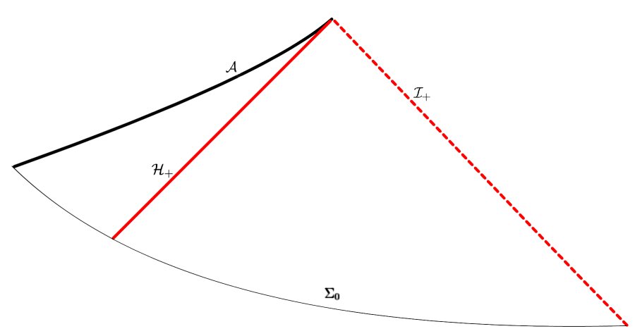
Figure 1: The Penrose diagram of the final space-time in Theorem 1.1 with initial hypersurface $\Sigma_{0}$, future space-like boundary $\mathcal{A}$, and $\mathscr{I}^{+}$ the complete future null infinity. The hypersurface $\mathcal{H}_{+}$ is the future event horizon of the final Kerr.

The proof of Theorem 1.1 is based on a limiting argument for a continuous family of such spacetimes $\mathcal{M}={}^{(ext)}\mathcal{M}\cup{\,{}^{(top)}\mathcal{M}}\cup{\,{}^{(int)}\mathcal{M}}$, represented graphically in Figure 2, together with a set of bootstrap assumptions (BA) for the connection and curvature coefficients, relative to the adapted frames. The main features of these spacetimes are as follows:

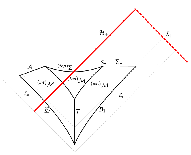
Figure 2: The Penrose diagram of a finite GCM admissible space-time $\mathcal{M}={}^{(ext)}\mathcal{M}\cup{\,{}^{(top)}\mathcal{M}}\cup{\,{}^{(int)}\mathcal{M}}$. The future boundary $\Sigma_{*}$ initiates at the GCM sphere $S_{*}$. The past boundary of $\mathcal{M}$, $\mathcal{B}_{1}\cup\underline{\mathcal{B}}_{1}$, is included in the initial layer $\mathcal{L}_{0}$, in which the spacetime is assumed given.

• The capstone of the entire construction is the sphere $S_{*}$, on the future boundary $\Sigma_{*}$ of ${}^{(ext)}\mathcal{M}$, which verifies a set of specific extrinsic and intrinsic conditions denoted by the acronym GCM.

• The spacelike hypersurface $\Sigma_{*}$, initialized at $S_{*}$, verifies a set of additional GCM conditions.

• Once $\Sigma_{*}$ is specified the whole GCM admissible spacetime $\mathcal{M}$ is determined by a more conventional construction, based on geometric transport type equations.

• The construction, which also allows us to specify adapted null frames, is made possible by the covariance properties of the Einstein vacuum equations.

• The past boundary $\mathcal{B}_{1}\cup\underline{\mathcal{B}}_{1}$ of $\mathcal{M}$, which is itself to be constructed, is included in the initial layer $\mathcal{L}_{0}$ in which the spacetime is assumed to be known, i.e. a small vacuum perturbation of a Kerr solution.

Assuming that a given finite, GCM admissible spacetime $\mathcal{M}$ saturates the bootstrap assumptions BA we reach a contradiction as follows:

• First, improve the BA for some of the components of the curvature tensor with respect to the frame. These verify equations (called Teukolsky equations) that decouple, up to terms quadratic in the perturbation, and are treated by wave equation methods.

• Use the information provided by these curvature coefficients together with the gauge choice on $\mathcal{M}$, induced by the GCM condition on $\Sigma_{*}$, to improve BA for all other Ricci and curvature components.

• Use these improved estimates to extend $\mathcal{M}$ to a strictly larger spacetime $\mathcal{M}^{\prime}$ and then construct a new GCM sphere $S_{*}^{\prime}$, a new boundary $\Sigma_{*}^{\prime}$ that initiates on $S_{*}^{\prime}$, and a new GCM admissible spacetime $\mathcal{M}^{\prime}$, with $\Sigma_{*}^{\prime}$ as the boundary, strictly larger than $\mathcal{M}$.

• The final spacetime $\big{(}\mathcal{M}_{\infty},{\bf g}_{\infty}\big{)}$, $\mathcal{M}_{\infty}={}^{(ext)}\mathcal{M}\cup{\,{}^{(int)}\mathcal{M}}$, derived in the proof of Theorem 1.1, is equipped with specified PG structures in both ${}^{(ext)}\mathcal{M}$ and ${\,{}^{(int)}\mathcal{M}}$. In particular, ${}^{(ext)}\mathcal{M}$ has an outgoing PG structure $\big{\{}(e_{3},e_{4};\mathcal{H}),r,\theta,u)\big{\}}$, as well as a set of $\ell=1$ basis $J^{(p)}$, for $p=+,0,-$, relative to each, the null connections and the curvature components have specified decay properties.

Remark 1.2.

The final state $\mathcal{M}_{\infty}$ verifies all the relevant properties described in Section 3.4 in [31] in which the precise version of Theorem 1.1 is given. In this paper, we are only interested in the limits at future null infinity, that is, we are only interested in ${}^{(ext)}\mathcal{M}_{\infty}$, the external part of $\mathcal{M}_{\infty}$. We refer to these as $\operatorname{KSAF^{+}}$ spacetimes, (see Definition 2.18 for more explanations). Since there is no danger of confusion, we simply denote them by $\mathcal{M}$. Thus, a $\operatorname{KSAF^{+}}$ spacetime $\mathcal{M}$ is future null complete and verifies all the properties of ${}^{(ext)}\mathcal{M}_{\infty}$ described in the main theorem of [31]. In particular $\operatorname{KSAF^{+}}$ spacetimes verify all the assumptions made in [29, 30, 40] concerning the existence of GCM spheres and GCM hypersurfaces.

Remark 1.3.

Section 3.8 of [31] contains various conclusions concerning the completeness of $\mathscr{I}^{+}$, the existence of a future event horizon, the definition of Bondi mass and angular momentum at null infinity, and the derivation of the Bondi mass loss formula. All these follow easily from the decay properties embodied in the main result of [31], (see Section 3.4.3 in [31]) and the basic equations of motion. Using the same ingredients, a memory-type result for the angular momentum was later derived by An-He-Shen [1]. The regularity of the horizon was recently proved by Chen-Klainerman [8]. It is important to note that all these conclusions remain true for the full sub-extremal range $|a|<m$ provided that similar decay estimates hold.

1.2 General covariant modulated (GCM) procedure

The GCM spheres introduced in [29, 30] play an essential role throughout this paper. For the sake of this introduction, we review the main definitions needed to understand the statements of the results of Section 1.3. A more comprehensive discussion of these is given in Section 2.

1.2.1 Null horizontal structures

We use in what follows the language of null horizontal structures $e_{3},e_{4},\mathcal{H}$ developed in [19] and [31] and summarized here in section 2.1. In a first approximation, we need the definitions of the Ricci coefficients $\chi,{\underline{\chi}},\zeta$, with the first two decomposed into $\widehat{\chi},\operatorname{tr}\chi,{}^{(a)}\operatorname{tr}\chi$ and, respectively, $\widehat{{\underline{\chi}}},\operatorname{tr}{\underline{\chi}},{}^{(a)}\operatorname{tr}{\underline{\chi}}$, and the curvature components $\beta,\rho,{}^{*}\rho,\underline{\beta}$. We also need the mass aspect functions

$$\mu:=-\operatorname{div}\zeta-\rho+\frac{1}{2}\widehat{\chi}\cdot\widehat{{\underline{\chi}}},\qquad\quad{\underline{\mu}}:=\operatorname{div}\zeta-\rho+\frac{1}{2}\widehat{\chi}\cdot\widehat{{\underline{\chi}}}.$$

Recall that in the canonical outgoing geodesic foliation of Schwarzschild, we have

$$\operatorname{tr}\chi=\frac{2}{r},\qquad\quad\operatorname{tr}{\underline{\chi}}=-\frac{2\Upsilon}{r},\quad\qquad\mu=\frac{2m}{r^{3}},$$ (1.1)

where we denoted

$$\Upsilon:=1-\frac{2m}{r}.$$ (1.2)

Note that $r$ and $m$ coincide with the area radius and Hawking mass of surfaces $S$ of fixed $r$, i.e.

$$r:=\sqrt{\frac{|S|}{4\pi}},\qquad\qquad\frac{2m}{r}:=1+\frac{1}{16\pi}\int_{S}\operatorname{tr}\chi\operatorname{tr}{\underline{\chi}}.$$

We now introduce the following definition of outgoing principle geodesic (PG) structure, which plays an essential role in this paper.

Definition 1.4.

An outgoing PG structure consists of a null pair $(e_{3},e_{4})$ and the induced horizontal structure $\mathcal{H}$, together with a scalar function r such that:

1. $e_{4}$ is a null outgoing geodesic vectorfield, i.e. ${\bf D}_{4}e_{4}=0$,

2. $r$ is an affine parameter, i.e. $e_{4}(r)=1$,

3. the gradient of $r$, defined by $\operatorname{grad}r:={\bf g}^{\alpha\beta}\partial_{\beta}r\partial_{\alpha}$, is perpendicular to $\mathcal{H}$.

Remark 1.5.

By abuse of language, we call an outgoing PG structure $\{S(u,r),(e_{3},e_{4},\mathcal{H})\}$ simply an outgoing PG $S(u,r)$–foliation. The asymptotic properties of $\operatorname{KSAF^{+}}$ spacetimes, mentioned in Remark 1.2, are defined relative to a given outgoing PG structure.

1.2.2 Deformations of spheres and frame transformations

We consider a spacetime region $(\mathcal{M},{\bf g})$ endowed with an outgoing PG $S(u,r)$–foliation. The construction of GCM spheres in [29, 30] was obtained by deforming a given background sphere $S(u,r)$ by a map $\Psi:S(u,r)\to S^{\prime}\subset\mathcal{M}$ of the form

$$\Psi(u,r,\theta^{1},\theta^{2})=\left(u+U(\theta^{1},\theta^{2}),r+R(\theta^{1},\theta^{2}),\theta^{1},\theta^{2}\right)$$ (1.3)

with $(U,R)$ smooth functions on $S$, vanishing at a fixed point of $S$, and $(\theta^{1},\theta^{2})$ spherical coordinates on $S$. Given such a deformation, we identify, at any point on $S^{\prime}$, two important null frames:

1. The null frame $(e_{3},e_{4},e_{1},e_{2})$ of the background outgoing PG foliation;

2. A new null frame $(e^{\prime}_{3},e^{\prime}_{4},e^{\prime}_{1},e^{\prime}_{2})$ adapted to $S^{\prime}$ (i.e. $e_{1}^{\prime}$, $e_{2}^{\prime}$ tangent to $S^{\prime}$), obtained according to the transformation formulae (1.4).

In general, two null frames $(e_{3},e_{4},e_{1},e_{2})$ and $(e_{3}^{\prime},e_{4}^{\prime},e_{1}^{\prime},e_{2}^{\prime})$ are related by a frame transformation as follows:

$$\begin{split}e_{4}^{\prime}&=\lambda\left(e_{4}+f^{b}e_{b}+\frac{1}{4}|f|^{2}e_{3}\right),\\ e_{a}^{\prime}&=\left(\delta_{ab}+\frac{1}{2}{\underline{f}}_{a}f_{b}\right)e_{b}+\frac{1}{2}{\underline{f}}_{a}e_{4}+\left(\frac{1}{2}f_{a}+\frac{1}{8}|f|^{2}{\underline{f}}_{a}\right)e_{3},\\ e_{3}^{\prime}&=\lambda^{-1}\left(\left(1+\frac{1}{2}f\cdot{\underline{f}}+\frac{1}{16}|f|^{2}|{\underline{f}}|^{2}\right)e_{3}+\left({\underline{f}}^{b}+\frac{1}{4}|{\underline{f}}|^{2}f^{b}\right)e_{b}+\frac{1}{4}|{\underline{f}}|^{2}e_{4}\right),\end{split}$$ (1.4)

where the scalar function $\lambda$ and the 1-forms $f$ and ${\underline{f}}$ are called the transition functions from $(e_{3},e_{4},e_{1},e_{2})$ to $(e_{3}^{\prime},e_{4}^{\prime},e_{1}^{\prime},e_{2}^{\prime})$.

1.2.3 Basis of $\ell=1$ modes

We introduce the following generalization of the $\ell=1$ spherical harmonics of the standard sphere, which are used to define the GCM conditions.

Definition 1.6.

On an $\varepsilon$–almost round sphere $(S,g^{S})$, in the sense of

$$\left\|K^{S}-\frac{1}{(r^{S})^{2}}\right\|_{L^{\infty}(S)}\leq\frac{\varepsilon}{(r^{S})^{2}},$$ (1.5)

where $K^{S}$ denotes the Gauss curvature of $S$ and $r^{S}$ denotes the area radius of $S$.

1. We define an $\varepsilon$–approximate basis of $\ell=1$ modes on $S$ to be a triplet of functions $J^{(p)}$ on $S$ verifying

   $$\begin{split}(r^{2}\Delta+2)J^{(p)}&=O(\varepsilon),\qquad p=0,+,-,\\ \frac{1}{|S|}\int_{S}J^{(p)}J^{(q)}&=\frac{1}{3}\delta_{pq}+O(\varepsilon),\qquad p,q=0,+,-,\\ \frac{1}{|S|}\int_{S}J^{(p)}&=O(\varepsilon),\qquad p=0,+,-,\end{split}$$ (1.6)

   where $\varepsilon>0$ is a sufficiently small constant.

2. Let $(\Phi,u)$ be the unique, up to isometries of $\mathbb{S}^{2}$, uniformization, as in Corollary 3.8 of [30], that is, a unique diffeomorphism $\Phi:\mathbb{S}^{2}\to S$ and a unique centered conformal factor $u$ s.t.

   $$\Phi^{\#}(g^{S})=(r^{S})^{2}e^{2u}\gamma_{0}.$$

   We define the canonical choice of $\varepsilon$–approximate basis of $\ell=1$ modes on $S$ by

   $$J^{S}:=J^{\mathbb{S}^{2}}\circ\Phi^{-1},$$

   where $J^{\mathbb{S}^{2}}$ denotes the standard $\ell=1$ spherical harmonic on round sphere.

Remark 1.7.

On an $\varepsilon$–almost round sphere $(S,g^{S})$, the canonical choice of $\varepsilon$–approximate basis $J^{(S,p)}$ of $\ell=1$ modes on $S$ satisfy an addition property

$$\frac{1}{|S|}\int_{S}J^{(S,p)} =0,\qquad p=0,+,-.$$

This is a simple consequence of the centered (balancing) condition of the conformal factor $u$ in the definition.

Assuming the existence of such a basis $J^{(p)}$, $p\in\{-,0,+\}$, we define, for any scalar function $h$ on $S$,

$$(h)^{S}_{\ell=1}:=\left\{\frac{1}{|S|}\int_{S}hJ^{(p)},\quad p=-,0,+\right\}.$$ (1.7)

A scalar function $h$ on $S$ is said to be supported on $\ell\leq 1$ modes, i.e. $(h)^{S}_{\ell\geq 2}=0$, if there exist constants $A_{0},B_{-},B_{0},B_{+}$ such that

$$h=A_{0}+B_{-}J^{(-)}+B_{0}J^{(0)}+B_{+}J^{(+)}.$$ (1.8)

1.2.4 GCM spheres and incoming geodesic foliation

The idea behind GCM spheres in perturbations of Kerr, is that of finding 2-surfaces verifying conditions as close as possible to (1.1). In fact, the GCM spheres are topological spheres ${\mathbf{S}}$ endowed with a null frame $(e_{3}^{\mathbf{S}},e_{4}^{\mathbf{S}},e_{1}^{\mathbf{S}},e_{2}^{\mathbf{S}})$ adapted to ${\mathbf{S}}$ (i.e. $e_{1}^{\mathbf{S}},e_{2}^{\mathbf{S}}$ tangent to ${\mathbf{S}}$), relative to which the null expansions $\operatorname{tr}\chi^{\mathbf{S}}$, $\operatorname{tr}{\underline{\chi}}^{\mathbf{S}}$ and mass aspect function $\mu^{\mathbf{S}}$ satisfy:

$$\operatorname{tr}\chi^{\mathbf{S}}-\frac{2}{r^{\mathbf{S}}}=0,\qquad\left(\operatorname{tr}{\underline{\chi}}^{\mathbf{S}}+\frac{2\Upsilon^{\mathbf{S}}}{r^{\mathbf{S}}}\right)_{\ell\geq 2}=0,\qquad\left(\mu^{\mathbf{S}}-\frac{2m^{\mathbf{S}}}{(r^{\mathbf{S}})^{3}}\right)_{\ell\geq 2}=0,$$ (1.9)

where $r^{\mathbf{S}}$ and $m^{\mathbf{S}}$ denote the area radius and Hawking mass of ${\mathbf{S}}$ and $\Upsilon^{\mathbf{S}}$ is defined as in (1.2). A GCM sphere is called an intrinsic GCM sphere if in additional to (1.9), it satisfies:

$$\operatorname{tr}{\underline{\chi}}^{\mathbf{S}}=-\frac{2\Upsilon^{\mathbf{S}}}{r^{\mathbf{S}}},\qquad\qquad(\operatorname{div}^{\mathbf{S}}\beta^{\mathbf{S}})_{\ell=1}=0,$$ (1.10)

w.r.t. the canonical choice of $\varepsilon$–approximate basis of $\ell=1$ modes of ${\mathbf{S}}$. Note that all the quantities we have introduced above, based on the definitions made in Section 1.2.1, are well defined on a given sphere. We now recall the definition of an incoming geodesic foliation. To this end, we need to define the transverse Ricci coefficients, see Section 2.1,

$$\eta_{a}=\frac{1}{2}{\bf g}({\bf D}_{3}e_{4},e_{a}),\qquad{\underline{\xi}}_{a}=\frac{1}{2}{\bf g}({\bf D}_{3}e_{3},e_{a}),\qquad{\underline{\omega}}=\frac{1}{4}{\bf g}({\bf D}_{3}e_{3},e_{4}).$$

Recall that the incoming geodesic conditions (see Sections 2.3–2.4 in [31]) are given by:

$$\eta=0,\qquad\quad{\underline{\xi}}=0,\qquad\quad{\underline{\omega}}=0.$$ (1.11)

Remark 1.8.

Emanating from an intrinsic GCM sphere ${\mathbf{S}}$, we can construct an incoming null cone ${\underline{C}}$, endowed with an incoming geodesic foliation. We have by construction that (1.9) and (1.10) hold on the last sphere ${\mathbf{S}}$ while (1.11) holds on the null cone ${\underline{C}}$.

1.3 First version of main results

We are now ready to state simple versions of our main results and discuss the main ideas in their proofs.

1.3.1 Regularity of conformal metric up to $\mathscr{I}^{+}$

Let $(\mathcal{M},{\bf g})$ be a $\operatorname{KSAF^{+}}$ spacetime as defined in Remark 1.2. We denote $(\widetilde{\mathcal{M}},\widetilde{{\bf g}})$ its Penrose compactification:

$$\widetilde{\mathcal{M}}:=\mathcal{M}\cup\mathscr{I}^{+},\qquad\quad\widetilde{{\bf g}}:=\varrho^{2}{\bf g}.$$ (1.12)

with $\varrho:=r^{-1}$ the boundary defining function and the future null infinity $\mathscr{I}^{+}$ is defined by:

$$\mathscr{I}^{+}:=\{\varrho=0\}.$$

Theorem 1.9.

Let $(\mathcal{M},{\bf g})$ be a $\operatorname{KSAF^{+}}$ spacetime and let $(\widetilde{\mathcal{M}},\widetilde{{\bf g}})$ be the compactified spacetime defined in (1.12). Then we have

$$\widetilde{{\bf g}}\in C^{{k_{small}}}(\mathcal{M})\cap C^{1,\frac{1}{2}+\delta_{dec}}(\widetilde{\mathcal{M}}),$$

where ${k_{small}}$ is an integer that denotes the regularity of the decay estimates of [31] and $0<\delta_{dec}\ll 1$ is a fixed small constant.

Theorem 1.9 is restated as Theorem 4.7 in Section 4. The proof is based on the asymptotic behaviors of the metric components of $\operatorname{KSAF^{+}}$ spacetimes.

1.3.2 Limiting GCM (LGCM) foliation on $\mathscr{I}^{+}$

The following theorem shows the existence of a canonical foliation on the future null infinity $\mathscr{I}^{+}$, which is called a Limiting GCM (LGCM) foliation.

Theorem 1.10.

Let $(\mathcal{M},{\bf g})$ be a $\operatorname{KSAF^{+}}(a_{f},m_{f})$ spacetime, endowed with a background outgoing PG $S(u,r)$–foliation. Then, there exists a sphere foliation $S^{\prime}(u^{\prime},r^{\prime})$ and a null frame $(e^{\prime}_{3},e^{\prime}_{4},e_{1}^{\prime},e_{2}^{\prime})$ near $\mathscr{I}^{+}$, relative to which the Ricci coefficients and curvature components have the following asymptotic behavior:

$$\begin{split}\lim_{u\to\infty}\lim_{C_{u},r\to\infty}r^{2}\left(\operatorname{tr}\chi^{\prime}-\frac{2}{r^{\prime}}\right)&=0,\qquad\quad\;\,\lim_{u\to\infty}\lim_{C_{u},r\to\infty}r^{2}\left(\operatorname{tr}{\underline{\chi}}^{\prime}+\frac{2}{r^{\prime}}\right)=4m_{f},\\ \lim_{u\to\infty}\lim_{C_{u},r\to\infty}(r^{3}\mu^{\prime})_{\ell\geq 2}&=0,\qquad\qquad\quad\,\lim_{u\to\infty}\lim_{C_{u},r\to\infty}(\operatorname{div}^{\prime}\beta^{\prime})_{\ell=1}=0,\\ \lim_{C_{u},r\to\infty}\left(r^{2}\,{}^{(a)}\operatorname{tr}\chi^{\prime},r^{2}\,{}^{(a)}\operatorname{tr}{\underline{\chi}}^{\prime}\right)&=0,\qquad\qquad\lim_{u\to\infty}\lim_{C_{u},r\to\infty}r^{5}(\operatorname{div}^{\prime}\beta^{\prime})_{\ell=1}=2a_{f}m_{f},\end{split}$$ (1.13)

where the modes are taken w.r.t. to an approximate basis of $\ell=1$ modes $J^{(p)}$ introduced in Definition 1.6. We also have the following asymptotic behavior:

$$\lim_{C_{u},r\to\infty}(r\eta,r{\underline{\xi}},r{\underline{\omega}})=0.$$ (1.14)

Moreover, a sphere foliation near $\mathscr{I}^{+}$ that satisfies (1.13) and (1.14) is called a Limiting GCM (LGCM) foliation.

Theorem 1.10 is restated as Theorem 5.4 and proved in Section 5.4, which constructs the desired foliation from the background foliation of $(\mathcal{M},{\bf g})$. The construction is based on a limiting process, which shows that a sequence of incoming null cones, emanating from intrinsic GCM spheres, endowed with incoming geodesic foliation, converges to the desired foliation on $\mathscr{I}^{+}$.

1.3.3 Absence of supertranslation and spatial translation

The next theorem illustrates the uniqueness of the LGCM foliation defined in Theorem 1.10.

Theorem 1.11.

Let $(\mathcal{M},{\bf g})$ be a $\operatorname{KSAF^{+}}$ spacetime. Any two LGCM foliations of $(\mathcal{M},{\bf g})$ near $\mathscr{I}^{+}$, differ by a translation along $\mathscr{I}^{+}$. More precisely, denoting $(f,{\underline{f}},\lambda)$ the transition functions from the frame of the first LGCM to that of the second, as defined by (1.4), we must have

$$\lim_{C_{u},r\to\infty}(rf,r{\underline{f}},r\overset{\circ}{\lambda})=0.$$ (1.15)

Theorem 1.11 is restated as Theorem 6.1 and proved in Section 6, based on the fact that, since the GCM conditions (1.13) hold for both LGCM foliations near $i^{+}$ we can derive an elliptic system for $(f,{\underline{f}},\lambda)$ near $i^{+}$, which implies that (1.15) holds near $i^{+}$. Since geodesic conditions (1.14) hold for both LGCM foliations, we obtain a transport system for $(f,{\underline{f}},\lambda)$ along $\mathscr{I}^{+}$, from which the uniqueness of $(f,{\underline{f}},\lambda)$ on $\mathscr{I}^{+}$ follows easily.

Remark 1.12.

The condition (1.15) implies that the physical quantities defined in two different LGCM foliations coincide with each other. This eliminates the supertranslation ambiguity and spatial translation, see Remark 6.2 for more explanations.

1.3.4 Physical laws on $\mathscr{I}^{+}$

The uniqueness of the LGCM foliation, proved in Theorem 1.11, allows us to make unambiguous definitions of the main physical quantities (energy, linear and angular momentum and center of mass) at null infinity.

Definition 1.13.

Relative to the associated LGCM foliation of a $\operatorname{KSAF^{+}}$ spacetime, constructed by Theorem 1.10, we introduce the following limiting quantities

• Define the shear ${}^{({LG})}\Theta$ and news ${}^{({LG})}{\underline{\Theta}}$ at $\mathscr{I}^{+}$:

  $${}^{({LG})}\Theta:=\lim_{C_{u},r\to\infty}r^{2}\,{}^{({LG})}\widehat{\chi},\qquad\quad{}^{({LG})}{\underline{\Theta}}:=\lim_{C_{u},r\to\infty}r\,{}^{({LG})}\widehat{{\underline{\chi}}}.$$ (1.16)

• Define the energy ${}^{({LG})}\mathcal{E}$, linear momentum ${}^{({LG})}\mathcal{P}$, center of mass ${}^{({LG})}\mathcal{C}$ and angular momentum ${}^{({LG})}\mathcal{J}$ as follows:

  $$\begin{split}{}^{({LG})}\mathcal{E}&:=\lim_{C_{u},r\to\infty}\frac{r^{3}}{2}\left({}^{({LG})}\mu+{}^{({LG})}{\underline{\mu}}\right)_{\ell=0},\\ {}^{({LG})}\mathcal{P}&:=\lim_{C_{u},r\to\infty}\frac{r^{3}}{2}\left({}^{({LG})}\mu+{}^{({LG})}{\underline{\mu}}\right)_{\ell=1},\\ {}^{({LG})}\mathcal{C}&:=\lim_{C_{u},r\to\infty}r^{5}\left({}^{({LG})}\operatorname{div}{}^{({LG})}\beta\right)_{\ell=1},\\ {}^{({LG})}\mathcal{J}&:=\lim_{C_{u},r\to\infty}r^{5}\left({}^{({LG})}\operatorname{curl}{}^{({LG})}\beta\right)_{\ell=1}.\end{split}$$ (1.17)

• For any $1$–form $f$ and tensorfield $U$ satisfying

  $$\lim_{C_{u},r\to\infty}f=\mathscr{F},\qquad\quad\lim_{C_{u},r\to\infty}U={\mathscr{U}},$$

  we define the limiting differential operators:

  $$(\overset{\circ}{\operatorname{div}}\,,\overset{\circ}{\operatorname{curl}}\,)\mathscr{F}:=\lim_{C_{u},r\to\infty}r(\operatorname{div},\operatorname{curl})f,\qquad(\overset{\circ}{\nabla}_{3},\overset{\circ}{\nabla}){\mathscr{U}}:=\lim_{C_{u},r\to\infty}(\nabla_{3},r\nabla)U.$$ (1.18)

Remark 1.14.

The shear $\Theta$ and news ${\underline{\Theta}}$ defined in (1.16) describe the nonlinear terms in the evolution of physical quantities defined in (1.17), see Theorem 1.15 below. Note also that relative to a coordinates chart $(u,\theta,\varphi)$ on $\mathscr{I}^{+}$, the limiting differential operators $\overset{\circ}{\nabla}_{3}$ and $\overset{\circ}{\nabla}_{a}$ with $a=1,2$, defined in (1.18), are linear combinations of $\partial_{u}$, $\partial_{\theta}$ and $\partial_{\varphi}$.

We are now ready to describe the evolution of physical quantities along $\mathscr{I}^{+}$ in the LGCM foliation.

Theorem 1.15.

Let $(\mathcal{M},{\bf g})$ be a $\operatorname{KSAF^{+}}$ spacetime. Then in the LGCM foliation, the null energy, linear momentum, center of mass and angular momentum introduced in Definition 1.13 satisfy the following evolution equations:

$$\begin{split}\partial_{u}\left({}^{({LG})}\mathcal{E}\right)&=-\frac{1}{4}\left(\big{|}{}^{({LG})}{\underline{\Theta}}\big{|}^{2}\right)_{\ell=0},\\ \partial_{u}\left({}^{({LG})}\mathcal{P}\right)&=-\frac{1}{4}\left(\big{|}{}^{({LG})}{\underline{\Theta}}\big{|}^{2}\right)_{\ell=1},\\ \partial_{u}\left({}^{({LG})}\mathcal{C}\right)&={}^{({LG})}\mathcal{P}+\left(\frac{1}{2}{}^{({LG})}\Theta\cdot{}^{({LG})}{\underline{\Theta}}+{}^{({LG})}\overset{\circ}{\operatorname{div}}\,\left({}^{({LG})}\overset{\circ}{\operatorname{div}}\,{}^{({LG})}{\underline{\Theta}}\cdot{}^{({LG})}\Theta\right)\right)_{\ell=1},\\ \partial_{u}\left({}^{({LG})}\mathcal{J}\right)&=\left(\frac{1}{2}{}^{({LG})}\Theta\wedge{}^{({LG})}{\underline{\Theta}}+{}^{({LG})}\overset{\circ}{\operatorname{curl}}\,\left({}^{({LG})}\overset{\circ}{\operatorname{div}}\,{}^{({LG})}{\underline{\Theta}}\cdot{}^{({LG})}\Theta\right)\right)_{\ell=1},\end{split}$$ (1.19)

where all the modes are taken w.r.t. the $\ell=1$ basis $J^{(p)}$ of the LGCM foliation.

Theorem 1.15 is restated as Theorem 7.7 and proved in Section 7. The evolution laws in (1.19) follow by taking the limits of the null structure equations in the direction $e_{3}$.

Remark 1.16.

The first equation in (1.19) implies the Bondi mass loss formula. It was first derived and used by Christodoulou [11] in connection with his famous memory effect. The last equation in (1.19) was derived and used in [1] to derive an angular momentum memory type effect. See Remark 7.8 for more explanations about (1.19).

1.3.5 Gravitational wave recoil

Theorem 1.17.

Let $(\mathcal{M},{\bf g})$ be the final spacetime derived in the proof of Theorem 1.1 and let $\mathcal{L}_{0}$ be the initial layer region, endowed with a $S^{(0)}$–foliation, given as the initial assumption in [31]. Let $S(1,r)$ be a leaf of the LGCM foliation constructed in Theorem 1.10 and let $S^{(0)}_{1}$ be a leaf of the initial layer foliation that has a point common to $S(1,r)$. We define the center of mass on $S(1,r)$ and $S^{(0)}_{1}$ as in (1.17):

$$\mathcal{C}_{1}:=r^{5}(\operatorname{div}\beta)_{\ell=1,S(1,r)},\qquad\mathcal{C}^{(0)}_{1}:=(r^{(0)})^{5}\left(\operatorname{div}^{(0)}\beta^{(0)}\right)_{\ell=1,S^{(0)}}.$$

Then, we have

$$\mathcal{C}_{1}-\mathcal{C}^{(0)}_{1}=O\left(\varepsilon_{0}r^{\frac{1}{2}-\delta_{dec}}\right).$$

Theorem 1.17 is restated as Theorem 8.5 and proved in Section 8 by combining the evolution equations of the center of mass in (1.19) with the initial perturbation assumption of [31].

Remark 1.18.

Theorem 1.17 encodes the fact that there is a large displacement of the center of mass of the initial layer foliation relative to that of the LGCM foliation. This leads to non trivial technical difficulties encountered in the proof of Theorem M0 in [31]. The large deformation of the center of mass is sometimes referred to as gravitational wave recoil or black hole kick in the physical literature, see [16, 21, 47]. See also Remark 8.6 for more explanations.

Remark 1.19.

The initial assumption in [31] implies that

$$\operatorname{div}^{(0)}\beta^{(0)}=O\left(\frac{\varepsilon_{0}}{r^{\frac{9}{2}+\delta_{dec}}}\right).$$

Hence, we have

$$\mathcal{C}^{(0)}_{1}=(r^{(0)})^{5}\left(\operatorname{div}^{(0)}\beta^{(0)}\right)_{\ell=1,S^{(0)}}=O(\varepsilon_{0}r^{\frac{1}{2}-\delta_{dec}}),$$

which implies the non triviality of kick. However, under stronger assumptions of the decay rates of the initial data for a black hole stability problem, one can show that the black hole kick has size $O(\varepsilon_{0})$, see Theorem 8.8 for more details.

1.4 Structure of the paper

• In Section 2, we introduce the basic geometric setup and recall the fundamental notions and the basic equations. We also establish the null frame transformation formulae.

• In Section 3, we study the asymptotic behavior of the null Ricci and curvature components. More precisely, we prove the existence of their appropriate weighted limits and deduce their Taylor expansions in terms of $r^{-1}$ near future null infinity $\mathscr{I}^{+}$.

• In Section 4, we introduce the Penrose conformal compactification of the $\operatorname{KSAF^{+}}$ spacetime $(\mathcal{M},{\bf g})$, with $\mathscr{I}^{+}$ its future null boundary. We show that the regularity of the conformal metric up to $\mathscr{I}^{+}$ is determined by its decay properties in $r$.

• In Section 5, we recall the main definitions and results of the GCM spheres introduced in [29, 30] and construct a sequence of incoming null cones embedded in $(\mathcal{M},{\bf g})$, which converges to $\mathscr{I}^{+}$. We prove that in the limit they induce a canonical foliation on $\mathscr{I}^{+}$, called a Limiting GCM (LGCM) foliation.

• In Section 6, we show that the LGCM foliation defined in Section 5 is unique on $\mathscr{I}^{+}$ up to a trivial transformation. Thus, LGCM foliations exclude Pernrose’s supertranslation ambiguity and also the freedom of spatial translation on $\mathscr{I}^{+}$.

• In Section 7, we use LGCM foliation to define the null energy, linear momentum, center of mass and angular momentum on $\mathscr{I}^{+}$. In view of the uniqueness of LGCM foliation, these quantities are unambiguously defined. We derive the basic evolution laws for these physical quantities along null infinity and draw comparisons with the ones for the classical mechanics of isolated systems.

• In Section 8, we compare the center of mass for the initial layer foliation, introduced as the initial assumptions of [31] on $\mathcal{L}_{0}$, and the LGCM foliation of $\mathscr{I}^{+}$. We show that there is a large deformation of the two centers of mass near $\mathscr{I}^{+}\cap\mathcal{L}_{0}$. This phenomenon corresponds to a gravitational wave recoil, or black hole kick in the physics literature, see for example [16, 21, 47].

• In Appendix A, we recall the main equations and commutation identities in [19, 31] that are used in this paper. We also provide the proof of Theorem 3.9, which describes the asymptotic behavior of all geometric quantities near $\mathscr{I}^{+}$.

• In Appendix B, we summarize all the limiting quantities we defined in this paper for the convenience of the reader.

1.5 Acknowledgements

The authors are very grateful to Xinliang An, Elena Giorgi, Taoran He, Jérémie Szeftel, Mu-Tao Wang and Pin Yu for their interest in this work and for many helpful discussions and comments.

2 Preliminaries

We summarize the general formalism introduced in [19] and the main assumptions in [31], which will be used in this paper, see also Appendix A for more details.

2.1 Null horizontal structures

Let $(\mathcal{M},{\bf g})$ be a Lorentzian spacetime. Consider a fixed null pair of vectorfields $(e_{3},e_{4})$, i.e.

$${\bf g}(e_{3},e_{3})={\bf g}(e_{4},e_{4})=0,\qquad{\bf g}(e_{3},e_{4})=-2,$$

and denote by $\mathcal{H}$ the vector space of horizontal vectorfields $X$ on $\mathcal{M}$, i.e. ${\bf g}(e_{3},X)={\bf g}(e_{4},X)=0$. A null frame $(e_{3},e_{4},e_{1},e_{2})$ on $\mathcal{M}$ consists, in addition to the null pair $(e_{3},e_{4})$, of a choice of horizontal vectorfields $(e_{1},e_{2})$, such that

$${\bf g}(e_{a},e_{b})=\delta_{ab}\qquad a,b=1,2.$$

However, the commutator $[X,Y]$ of two horizontal vectorfields may not be horizontal. We say that the pair $(e_{3},e_{4})$ is integrable if $\mathcal{H}$ forms an integrable distribution, i.e. $X,Y\in\mathcal{H}$ implies $[X,Y]\in\mathcal{H}$. As is well known, the principal null pair in Kerr fails to be integrable, see also Remark 2.1. Given an arbitrary vectorfield $X$ we denote by ${}^{(h)}X$ its horizontal projection,

$${}^{(h)}X=X+\frac{1}{2}{\bf g}(X,e_{3})e_{4}+\frac{1}{2}{\bf g}(X,e_{4})e_{3}.$$

For any $X,Y\in\mathbf{O}(\mathcal{M})$ we define $\gamma(X,Y)={\bf g}(X,Y)$ and

$$\chi(X,Y)={\bf g}({\bf D}_{X}e_{4},Y),\qquad{\underline{\chi}}(X,Y)={\bf g}({\bf D}_{X}e_{3},Y).$$

Observe that $\chi$ and ${\underline{\chi}}$ are symmetric if and only if the horizontal structure is integrable. Indeed this follows easily from the formulae,

$$\chi(X,Y)-\chi(Y,X) ={\bf g}({\bf D}_{X}e_{4},Y)-{\bf g}({\bf D}_{Y}e_{4},X)=-{\bf g}(e_{4},[X,Y]),$$

$${\underline{\chi}}(X,Y)-{\underline{\chi}}(Y,X) ={\bf g}({\bf D}_{X}e_{3},Y)-{\bf g}({\bf D}_{Y}e_{3},X)=-{\bf g}(e_{3},[X,Y]).$$

We define their trace $\operatorname{tr}\chi$, $\operatorname{tr}{\underline{\chi}}$, and anti-trace ${}^{(a)}\operatorname{tr}\chi$, ${}^{(a)}\operatorname{tr}{\underline{\chi}}$ as follows

$$\operatorname{tr}\chi:=\delta^{ab}\chi_{ab},\qquad\operatorname{tr}{\underline{\chi}}:=\delta^{ab}{\underline{\chi}}_{ab},\qquad{}^{(a)}\operatorname{tr}\chi:=\in^{ab}\chi_{ab},\qquad{}^{(a)}\operatorname{tr}{\underline{\chi}}:=\in^{ab}{\underline{\chi}}_{ab}.$$

Accordingly, we decompose $\chi,{\underline{\chi}}$ as follows

$$\chi_{ab} =\widehat{\chi}_{ab}+\frac{1}{2}\delta_{ab}\operatorname{tr}\chi+\frac{1}{2}\in_{ab}{}^{(a)}\operatorname{tr}\chi,$$

$${\underline{\chi}}_{ab} =\widehat{{\underline{\chi}}}_{ab}+\frac{1}{2}\delta_{ab}\operatorname{tr}{\underline{\chi}}+\frac{1}{2}\in_{ab}{}^{(a)}\operatorname{tr}{\underline{\chi}}.$$

where $\widehat{\chi}$ and $\widehat{{\underline{\chi}}}$ are the symmetric traceless parts of $\chi$ and ${\underline{\chi}}$ respectively.

Remark 2.1.

The non integrability of $(e_{3},e_{4})$ corresponds to non vanishing ${}^{(a)}\operatorname{tr}\chi$ and ${}^{(a)}\operatorname{tr}{\underline{\chi}}$. This is the case of the principal null frame of Kerr for which ${}^{(a)}\operatorname{tr}\chi$ and ${}^{(a)}\operatorname{tr}{\underline{\chi}}$ are indeed non trivial. The quantities $\operatorname{tr}\chi$ and $\operatorname{tr}{\underline{\chi}}$ are also called null expansions.

We define the horizontal covariant operator $\nabla$ as follows:

$$\nabla_{X}Y:=^{(h)}({\bf D}_{X}Y)={\bf D}_{X}Y-\frac{1}{2}{\underline{\chi}}(X,Y)e_{4}-\frac{1}{2}\chi(X,Y)e_{3},\quad X,Y\in\mathcal{H}.$$

Note that,

$$\nabla_{X}Y-\nabla_{Y}X=[X,Y]-\frac{1}{2}\left({}^{(a)}\operatorname{tr}{\underline{\chi}}\,e_{4}+{}^{(a)}\operatorname{tr}\chi\,e_{3}\right)\in(X,Y).$$

Note that $\nabla$ acts like a Levi-Civita connection i.e., for all $X,Y,Z\in\mathcal{H}$,

$$Z\gamma(X,Y)=\gamma(\nabla_{Z}X,Y)+\gamma(X,\nabla_{Z}Y).$$

We can then define connection and curvature coefficients similar to those in the integrable case, as in [13].

Definition 2.2.

Given a null pair $(e_{3},e_{4})$ and $e_{a}$ a basis of the horizontal space $\mathcal{H}$ we define.

1. Ricci coefficients

   $${\underline{\chi}}_{ab} ={\bf g}({\bf D}_{a}e_{3},e_{b}),\quad\,\,\chi_{ab}={\bf g}({\bf D}_{a}e_{4},e_{b}),\quad\,\,\,\,{\underline{\xi}}_{a}=\frac{1}{2}{\bf g}({\bf D}_{3}e_{3},e_{a}),\quad\,\,\,\xi_{a}=\frac{1}{2}{\bf g}({\bf D}_{4}e_{4},e_{a}),$$

   $${\underline{\omega}} =\frac{1}{4}{\bf g}({\bf D}_{3}e_{3},e_{4}),\quad\,\,\omega=\frac{1}{4}{\bf g}({\bf D}_{4}e_{4},e_{3}),\quad{\underline{\eta}}_{a}=\frac{1}{2}{\bf g}({\bf D}_{4}e_{3},e_{a}),\quad\quad\eta_{a}=\frac{1}{2}{\bf g}({\bf D}_{3}e_{4},e_{a}),$$

   $$\zeta_{a} =\frac{1}{2}{\bf g}({\bf D}_{a}e_{4},e_{3}).$$

2. Curvature coefficients

   $$\alpha_{ab} =\mathbf{R}_{a4b4},\qquad\quad\,\beta_{a}=\frac{1}{2}\mathbf{R}_{a434},\qquad\quad\underline{\beta}_{a}=\frac{1}{2}\mathbf{R}_{a334},\qquad\quad\underline{\alpha}_{ab}=\mathbf{R}_{a3b3},$$

   $$\rho =\frac{1}{4}\mathbf{R}_{3434},\qquad\;\,{}^{*}\rho=\frac{1}{4}{}^{*}\mathbf{R}_{3434},$$

3. Mass aspect function and conjugate mass aspect function

   $$\mu:=-\operatorname{div}\zeta-\rho+\frac{1}{2}\widehat{\chi}\cdot\widehat{{\underline{\chi}}},\qquad{\underline{\mu}}:=\operatorname{div}\zeta-\rho+\frac{1}{2}\widehat{\chi}\cdot\widehat{{\underline{\chi}}}$$

4. We define the following complex notations according to [18]

   $$A:=\alpha+i{}^{*}\alpha,\quad B:=\beta+i{}^{*}\beta,\quad P:=\rho+i\sigma,\quad{\underline{B}}:=\underline{\beta}+i{}^{*}\underline{\beta},\quad{\underline{A}}:=\underline{\alpha}+i{}^{*}\underline{\alpha},$$

   and

   $$X =\chi+i{}^{*}\chi,\quad{\underline{X}}={\underline{\chi}}+i{}^{*}{\underline{\chi}},\quad H=\eta+i{}^{*}\eta,\quad\underline{H}={\underline{\eta}}+i{}^{*}{\underline{\eta}},\quad Z=\zeta+i{}^{*}\zeta,$$

   $$\Xi =\xi+i{}^{*}\xi,\quad\;\;{\underline{\Xi}}={\underline{\xi}}+i{}^{*}{\underline{\xi}}.$$

   In particular, note that

   $$\operatorname{tr}X=\operatorname{tr}\chi-i{}^{(a)}\operatorname{tr}\chi,\quad\widehat{X}=\widehat{\chi}+i{}^{*}\widehat{\chi},\quad\operatorname{tr}{\underline{X}}=\operatorname{tr}{\underline{\chi}}-i{}^{(a)}\operatorname{tr}{\underline{\chi}},\quad\widehat{{\underline{X}}}=\widehat{{\underline{\chi}}}+i{}^{*}\widehat{{\underline{\chi}}}.$$

2.2 Hodge systems

Definition 2.3.

For tensor fields defined on a $2$–sphere $S$, we denote by $\mathfrak{s}_{0}:=\mathfrak{s}_{0}(S)$ the set of pairs of scalar functions, $\mathfrak{s}_{1}:=\mathfrak{s}_{1}(S)$ the set of $1$–forms and $\mathfrak{s}_{2}:=\mathfrak{s}_{2}(S)$ the set of symmetric traceless $2$–tensors.

Definition 2.4.

Given $\xi\in\mathfrak{s}_{1}$, we define its Hodge dual

$${{}^{*}\xi}_{a}:=\in_{ab}\xi^{b}.$$

Clearly ${}^{*}\xi\in\mathfrak{s}_{1}$ and

$${}^{*}(^{*}\xi)=-\xi.$$

Given $U\in\mathfrak{s}_{2}$, we define its Hodge dual

$${{}^{*}U}_{ab}:=\in_{ac}{U^{a}}_{b}.$$

Observe that ${}^{*}U\in\mathfrak{s}_{2}$ and

$${}^{*}(^{*}U)=-U.$$

Definition 2.5.

Given $\xi,\eta\in\mathfrak{s}_{1}$, we denote

$$\xi\cdot\eta :=\delta^{ab}\xi_{a}\eta_{b},$$

$$\xi\wedge\eta :=\in^{ab}\xi_{a}\eta_{b},$$

$$(\xi\widehat{\otimes}\eta)_{ab} :=\xi_{a}\eta_{b}+\xi_{b}\eta_{a}-\delta_{ab}\xi\cdot\eta.$$

Given $\xi\in\mathfrak{s}_{1}$, $U\in\mathfrak{s}_{2}$, we denote

$$(\xi\cdot U)_{a}:=\delta^{bc}\xi_{b}U_{ac}.$$

Given $U,V\in\mathfrak{s}_{2}$, we denote

$$U\wedge V :=\in^{ab}U_{ac}V_{cb},$$

$$U\cdot V :=\delta^{ab}U_{ac}V_{cb}.$$

Definition 2.6.

For a given $\xi\in\mathfrak{s}_{1}$, we define the following differential operators:

$$\operatorname{div}\xi :=\delta^{ab}\nabla_{a}\xi_{b},$$

$$\operatorname{curl}\xi :=\in^{ab}\nabla_{a}\xi_{b},$$

$$(\nabla\widehat{\otimes}\xi)_{ab} :=\nabla_{a}\xi_{b}+\nabla_{b}\xi_{a}-\delta_{ab}(\operatorname{div}\xi).$$

Definition 2.7.

We define the following Hodge type operators:

• $d_{1}$ takes $\mathfrak{s}_{1}$ into $\mathfrak{s}_{0}$ and is given by:

  $$d_{1}\xi:=(\operatorname{div}\xi,\operatorname{curl}\xi),$$

• $d_{2}$ takes $\mathfrak{s}_{2}$ into $\mathfrak{s}_{1}$ and is given by:

  $$(d_{2}U)_{a}:=\nabla^{b}U_{ab},$$

• $d_{1}^{*}$ takes $\mathfrak{s}_{0}$ into $\mathfrak{s}_{1}$ and is given by:

  $$d_{1}^{*}(f,f_{*})_{a}:=-\nabla_{a}f+\in_{ab}\nabla_{b}f_{*},$$

• $d_{2}^{*}$ takes $\mathfrak{s}_{1}$ into $\mathfrak{s}_{2}$ and is given by:

  $$d_{2}^{*}\xi:=-\frac{1}{2}\nabla\widehat{\otimes}\xi.$$

Proposition 2.8.

We have the following identities:

$$\begin{split}d_{1}^{*}d_{1}&=-\Delta_{1}+\mathbf{K},\qquad\qquad d_{1}d_{1}^{*}=-(\Delta_{0},\Delta_{0}),\\ d_{2}^{*}d_{2}&=-\frac{1}{2}\Delta_{2}+\mathbf{K},\qquad\quad\;d_{2}d_{2}^{*}=-\frac{1}{2}(\Delta_{1}+\mathbf{K}).\end{split}$$ (2.1)

where $\mathbf{K}$ denotes the Gauss curvature on $S$.

Proof.

See for example (2.2.2) in [13]. ∎

Definition 2.9.

We define derivatives of complex quantities as follows

• For two scalar functions $u$ and $v$, we define

  $$\mathcal{D}(u+iv):=(\nabla+i{}^{*}\nabla)(u+iv).$$

• For a 1-form $f$, we define

  $$\mathcal{D}\cdot(f+i{}^{*}f):=(\nabla+i{}^{*}\nabla)\cdot(f+i{}^{*}f),$$

  $$\mathcal{D}\widehat{\otimes}(f+i{}^{*}f):=(\nabla+i{}^{*}\nabla)\widehat{\otimes}(f+i{}^{*}f).$$

• For a symmetric traceless 2-form $u$, we define

  $$\mathcal{D}\cdot(U+i{}^{*}U):=(\nabla+i{}^{*}\nabla)\cdot(U+i{}^{*}U).$$

Proposition 2.10.

The following statements hold for all $p\in(1,+\infty)$:

1. Let $\phi\in\mathfrak{s}_{0}$ be a solution of $\Delta\phi=f$. Then, we have

   $$\|\nabla^{2}\phi\|_{L^{p}}+r^{-1}\|\nabla\phi\|_{L^{p}}+r^{-2}\|\phi-\overline{\phi}\|_{L^{p}} \lesssim\|f\|_{L^{p}}.$$

2. Let $\phi\in\mathfrak{s}_{0}$ be a solution of $\left(\Delta+\frac{2}{r^{2}}\right)\phi=f$. Then, we have

   $$\|\nabla^{2}\phi\|_{L^{p}}+r^{-1}\|\nabla\phi\|_{L^{p}}+r^{-2}\|\phi\|_{L^{p}} \lesssim\|f\|_{L^{p}}+r^{-2}|(\phi)_{\ell=1}|.$$

3. Let $\xi\in\mathfrak{s}_{1}$ be a solution of $d_{1}\xi=(f,f_{*})$. Then we have

   $$\|\nabla\xi\|_{L^{p}}+r^{-1}\|\xi\|_{L^{p}}\lesssim\|(f,f_{*})\|_{L^{p}}.$$

4. Let $U\in\mathfrak{s}_{2}$ be a solution of $d_{2}U=f$. Then we have

   $$\|\nabla U\|_{L^{p}}+r^{-1}\|U\|_{L^{p}}\lesssim\|f\|_{L^{p}}.$$

Proof.

See Corollary 2.3.1.1 in [13]. ∎

Definition 2.11.

We define the following weighted differential operator

$$\mathfrak{d}=(\nabla_{3},r\nabla_{4},\not{\mathfrak{d}}),$$

with $\not{\mathfrak{d}}$ defined as follows:

$$\not{\mathfrak{d}}(f,f_{*}) :=rd_{1}^{*}(f,f_{*}),\qquad\forall(f,f_{*})\in\mathfrak{s}_{0},$$

$$\not{\mathfrak{d}}\xi :=rd_{1}\xi,\qquad\qquad\qquad\;\forall\xi\in\mathfrak{s}_{1},$$

$$\not{\mathfrak{d}}U :=rd_{2}U,\qquad\qquad\quad\;\;\;\forall U\in\mathfrak{s}_{2}.$$

Moreover, for any quantity $X$, we denote

$$\not{\mathfrak{d}}^{\leq k}X:=\left(X,\,\not{\mathfrak{d}}X,\,\not{\mathfrak{d}}^{2}X,\ldots,\,\not{\mathfrak{d}}^{k}X\right),\qquad k\in\mathbb{N}.$$ (2.2)

We now introduce the definition of the approximate basis of $\ell=1$ modes on almost round spheres, which plays an essential role throughout this paper.

Definition 2.12.

On an $\varepsilon$-almost round sphere $(S,g^{S})$, in the sense of

$$\left\|K^{S}-\frac{1}{(r^{S})^{2}}\right\|_{L^{\infty}(S)}\leq\frac{\varepsilon}{(r^{S})^{2}}.$$ (2.3)

1. We define an $\varepsilon$–approximate basis of $\ell=1$ modes on $S$ to be a triplet of functions $J^{(p)}$ on $S$ verifying

   $$\begin{split}(r^{2}\Delta+2)J^{(p)}&=O(\varepsilon),\qquad p=0,+,-,\\ \frac{1}{|S|}\int_{S}J^{(p)}J^{(q)}&=\frac{1}{3}\delta_{pq}+O(\varepsilon),\qquad p,q=0,+,-,\\ \frac{1}{|S|}\int_{S}J^{(p)}&=O(\varepsilon),\qquad p=0,+,-,\end{split}$$ (2.4)

   where $\varepsilon>0$ is a sufficiently small constant.

2. Let $(\Phi,u)$ be the unique, up to isometries of $\mathbb{S}^{2}$, uniformization in Corollary 3.8. of [30], that is, a unique diffeomorphism $\Phi:\mathbb{S}^{2}\to S$ and a unique centered conformal factor $u$ s.t.

   $$\Phi^{\#}(g^{S})=(r^{S})^{2}e^{2u}\gamma_{0}.$$

   We define the canonical choice of $\varepsilon$–approximate basis of $\ell=1$ modes on $S$ by

   $$J^{S}:=J^{\mathbb{S}^{2}}\circ\Phi^{-1},$$

   where $J^{\mathbb{S}^{2}}$ denotes the standard $\ell=1$ spherical harmonic on round sphere.

Proposition 2.13.

For an $\varepsilon$–approximate basis of $\ell=1$ modes $J^{(p)}$ defined in Definition 2.12, we have

$$d_{2}^{*}d_{1}^{*}J^{(p)}=r^{-2}O(\varepsilon).$$ (2.5)

Proof.

See Lemma 5.37 in [31]. ∎

Definition 2.14.

Given a scalar function $f$ defined on a sphere $S$, we define the $\ell=1$ modes of $f$ w.r.t. a choice of $\varepsilon$–approximate basis of $\ell=1$ modes $J^{(p)}$ by the triplet

$$(f)_{\ell=1}:=\left\{\frac{1}{|S|}\int_{S}fJ^{(p)},\quad p=0,+,-\right\}.$$

2.3 Outgoing PG structures

We now recall the definition of outgoing Principal Geodesic (PG) structure, which was introduced and developed in Chapter 2 of [31].

Definition 2.15.

An outgoing PG structure consists of a null pair $(e_{3},e_{4})$ and the induced horizontal structure $\mathcal{H}$, together with a scalar function r such that:

1. $e_{4}$ is a null outgoing geodesic vectorfield, i.e. ${\bf D}_{4}e_{4}=0$,

2. $r$ is an affine parameter, i.e. $e_{4}(r)=1$,

3. the gradient of $r$, defined by $\operatorname{grad}r:={\bf g}^{\alpha\beta}\partial_{\beta}r\partial_{\alpha}$, is perpendicular to $\mathcal{H}$.

Lemma 2.16.

Given an outgoing PG structure as above, we have

$$\xi=0,\qquad\xi=0,\qquad{\underline{\eta}}+\zeta=0.$$

Proof.

See Lemma 2.17 in [31]. ∎

Remark 2.17.

By abuse of language, we call an outgoing PG structure $\{S(u,r),(e_{3},e_{4},\mathcal{H})\}$ simply an outgoing PG $S(u,r)$–foliation.

2.4 $\operatorname{KSAF^{+}}$ spacetime $(\mathcal{M},{\bf g})$

As mentioned in Remark 1.2, all our results, (except those in Section 8), apply to any $\operatorname{KSAF^{+}}$ spacetime $(\mathcal{M},{\bf g})$, which verifies the same properties as the final spacetime ${}^{(ext)}\mathcal{M}_{\infty}$ in Theorem 1.1. We state below the definition of a $\operatorname{KSAF^{+}}$ spacetime, which contains some of the main features of $\mathcal{M}$. More information can be found in Chapter 2 of [31].

Definition 2.18.

A spacetime $(\mathcal{M},{\bf g})$ is called a Klainerman-Szeftel Asymptotically Flat Future Complete spacetime with final parameters $(a,m)$ $(\operatorname{KSAF^{+}}(a,m)$ spacetime$)$, if it satisfies the following properties:

• $\mathcal{M}$ is equipped with an outgoing PG structure $\{S(u,r),(e_{3},e_{4};\mathcal{H})\}$ in the sense of Defintion 2.15.

• $\mathcal{M}$ is endowed with a pair of constants $(a,m)$.

• $\mathcal{M}$ is endowed with a scalar function $q:=r+ia\cos\theta$, with $\theta$ a scalar function satisfying

  $$e_{4}(\theta)=0.$$

• $\mathcal{M}$ is endowed with complex horizontal 1-forms $\mathfrak{J}$ and $\mathfrak{J}_{\pm}$ satisfying

  $$\nabla_{4}(q\mathfrak{J})=0,\qquad\qquad\nabla_{4}(q\mathfrak{J}_{\pm})=0.$$ (2.6)

• $\mathcal{M}$ is endowed with a retarded time function $u$ verifying $e_{4}(u)=0$.

• The initial layer region is defined by:

  $$\mathcal{L}_{0}:=\left\{p\in\mathcal{M}\big{/}\,0\leq u(p)\leq 3\right\}.$$

• Specific decay rates in $u$ and $r$ hold for all linearized Ricci and curvature coefficients Moreover precisely, the following decay estimates hold on $\mathcal{M}$:

  $$\begin{split}|\mathfrak{d}^{\leq{k_{small}}}(A,B)|&\lesssim\frac{\varepsilon_{0}}{r^{\frac{7}{2}+\delta_{dec}}},\\ \left|\mathfrak{d}^{\leq{k_{small}}}\left(\widecheck{\operatorname{tr}X},\,\widehat{X},\,\widecheck{Z},\,\widecheck{\operatorname{tr}{\underline{X}}},r\widecheck{P}\right)\right|&\lesssim\frac{\varepsilon_{0}}{r^{2}u^{\frac{1}{2}+\delta_{dec}}},\\ \left|\mathfrak{d}^{\leq{k_{small}}}(\widecheck{H},\,\widehat{{\underline{X}}},\,\widecheck{{\underline{\omega}}},\,{\underline{\Xi}},\,r{\underline{B}},{\underline{A}})\right|&\lesssim\frac{\varepsilon_{0}}{ru^{1+\delta_{dec}}},\end{split}$$ (2.7)

  where $\varepsilon_{0}$ is a constant small enough which describe the size of perturbation while ${k_{small}}$ is a sufficient large integer and $\delta_{dec}>0$ is a sufficiently small constant, which are used to describe the decay estimates in [31].

• The spacetime $(\mathcal{M},{\bf g})$ is covered by three coordinate systems:

  • in the $(u,r,\theta,\varphi)$ coordinates system, we have for $\frac{\pi}{4}<\theta<\frac{3\pi}{4}$,

    $${\bf g}={\bf g}_{a,m}+\Big{(}du,dr,rd\theta,r\sin\theta d\varphi\Big{)}^{2}O\left(\frac{\varepsilon_{0}}{u^{1+\delta_{dec}}}\right),$$

  • in the $(u,r,x^{1},x^{2})$ coordinates system, with $x^{1}=J^{(+)}$ and $x^{2}=J^{(-)}$, we have, for $0\leq\theta<\frac{\pi}{3}$ and for $\frac{2\pi}{3}<\theta\leq\pi$,

    $${\bf g} ={\bf g}_{a,m}+\Big{(}du,dr,rdx^{1},rdx^{2}\Big{)}^{2}O\left(\frac{\varepsilon_{0}}{u^{1+\delta_{dec}}}\right).$$

    See Section 3.4.3 in [31] and Proposition 2.22 below for more details.

Remark 2.19.

In the sequel, a $\operatorname{KSAF^{+}}(a,m)$ spacetime $(\mathcal{M},{\bf g})$ is simply called a $\operatorname{KSAF^{+}}$ spacetime if we do not need to describe its parameters $(a,m)$.

2.5 Schematic notation $\Gamma_{g}$ and $\Gamma_{b}$

Definition 2.20.

The Ricci coefficients and curvature components on $\mathcal{M}$ can be divided into the following groups:

1. The set $\Gamma_{g}$ with

   $$\Gamma_{g} :=\Big{\{}rB,\quad rA,\quad r\Xi,\quad\omega,\quad\widecheck{\underline{H}},\quad\widecheck{\operatorname{tr}X},\quad\widehat{X},\quad\widecheck{Z},\quad r\widecheck{P},\quad\widecheck{\operatorname{tr}{\underline{X}}}\Big{\}}.$$

2. The set $\Gamma_{b}=\Gamma_{b,1}\cup\Gamma_{b,2}\cup\Gamma_{b,3}\cup\Gamma_{b,4}$ with

   $$\Gamma_{b,1} :=\Big{\{}\widecheck{H},\quad\widehat{{\underline{X}}},\quad\widecheck{{\underline{\omega}}},\quad{\underline{\Xi}},\quad r{\underline{B}},\quad{\underline{A}}\Big{\}},$$

   $$\Gamma_{b,2} :=\Big{\{}r^{-1}\widecheck{e_{3}(r)},\quad\widecheck{\mathcal{D}q},\quad\widecheck{\mathcal{D}\overline{q}},\quad\widecheck{\mathcal{D}u},\quad r^{-1}\widecheck{e_{3}(u)}\Big{\}},$$

   $$\Gamma_{b,3} :=\Big{\{}\widecheck{\mathcal{D}(J^{(0)})},\quad\widecheck{\mathcal{D}(J^{(\pm)})},\quad e_{3}(J^{(0)}),\quad\widecheck{e_{3}(J^{(\pm)})}\Big{\}},$$

   $$\Gamma_{b,4} :=\left\{r\widecheck{\overline{\mathcal{D}}\cdot\mathfrak{J}},\quad r\mathcal{D}\widehat{\otimes}\mathfrak{J},\quad r\widecheck{\nabla_{3}\mathfrak{J}},\quad r\widecheck{\overline{\mathcal{D}}\cdot\mathfrak{J}_{\pm}},\quad r\mathcal{D}\widehat{\otimes}\mathfrak{J}_{\pm},\quad r\widecheck{\nabla_{3}\mathfrak{J}_{\pm}}\right\}.$$

Using the schematic notation $\Gamma_{g}$ and $\Gamma_{b}$, the decay estimates in a $\operatorname{KSAF^{+}}$ spacetime can be summarized in the following proposition.

Proposition 2.21.

Let $(\mathcal{M},{\bf g})$ be a $\operatorname{KSAF^{+}}$ spacetime endowed with an outgoing PG structure. Then, we have for $k\leq{k_{small}}$,

$$\sup_{\mathcal{M}}\Big{(}r^{\frac{7}{2}+\delta_{dec}}|\mathfrak{d}^{k}(A,B)|+r^{4}u^{1+\delta_{dec}}|\mathfrak{d}^{k-1}\nabla_{3}(A,B)|\Big{)} \lesssim\varepsilon_{0},$$

$$\sup_{\mathcal{M}}\Big{(}ru^{1+\delta_{dec}}|\mathfrak{d}^{k}\Gamma_{b}|+r^{2}u^{\frac{1}{2}+\delta_{dec}}|\mathfrak{d}^{k}\Gamma_{g}|+r^{2}u^{1+\delta_{dec}}|\mathfrak{d}^{k-1}\nabla_{3}\Gamma_{g}|\Big{)} \lesssim\varepsilon_{0}.$$

Proof.

See Proposition 6.49 in [31]. ∎

Proposition 2.22.

The spacetime $\operatorname{KSAF^{+}}$ spacetime $(\mathcal{M},{\bf g})$ is covered by three coordinate charts $\{(u,r,\theta,\varphi):\frac{\pi}{4}<\theta<\frac{3\pi}{4}\}$, $\{(u,r,x^{1},x^{2}):0\leq\theta<\frac{\pi}{3}\}$ and $\{(u,r,x^{1},x^{2}):\frac{2\pi}{3}<\theta\leq\pi\}$ where $x^{1}=\sin\theta\cos\varphi$ and $x^{2}=\sin\theta\sin\varphi$. More precisely, we have:

• in the $(u,r,\theta,\varphi)$ coordinates system for $\frac{\pi}{4}<\theta<\frac{3\pi}{4}$, ${\bf g}$ is given by:

  $${\bf g}= -2(du+dr)du+\left(1+\frac{2mr}{|q|^{2}}\right)\Big{(}du-a(\sin\theta)^{2}d\varphi\Big{)}^{2}+|q|^{2}\Big{[}(d\theta)^{2}+(\sin\theta)^{2}(d\varphi)^{2}\Big{]}$$

  $$+\Big{(}du,dr,rd\theta,r\sin\theta d\varphi\Big{)}^{2}(\sin\theta)^{-2}(r\Gamma_{b,2}\cup r\Gamma_{b,3}\cup r\Gamma_{b,4});$$

• in the $(u,r,x^{1},x^{2})$ coordinates system for $0\leq\theta<\frac{\pi}{3}$ or $\frac{2\pi}{3}<\theta\leq\pi$, ${\bf g}$ is given by

  $${\bf g} =-2(du+dr)du+\left(1+\frac{2mr}{|q|^{2}}\right)\Big{(}du-a(-x^{2}dx^{1}+x^{1}dx^{2})\Big{)}^{2}$$

  $$+\frac{|q|^{2}}{1-(x^{1})^{2}-(x^{2})^{2}}\Bigg{[}\Big{(}1-(x^{2})^{2}\Big{)}(dx^{1})^{2}+2x^{1}x^{2}dx^{1}dx^{2}+\Big{(}1-(x^{1})^{2}\Big{)}(dx^{2})^{2}\Bigg{]}$$

  $$+\Big{(}du,dr,rdx^{1},rdx^{2}\Big{)}^{2}(\cos\theta)^{-2}(r\Gamma_{b,2}\cup r\Gamma_{b,3}\cup r\Gamma_{b,4});$$

• in the $(u,r,\theta,\varphi)$ coordinates system for $\frac{\pi}{4}<\theta<\frac{3\pi}{4}$, ${\bf g}^{-1}$ is given by:

  $${\bf g}^{-1}={\bf g}^{-1}_{a,m}+\begin{pmatrix}r^{-2}&1&r^{-2}&r^{-2}\\ 1&1&r^{-1}&r^{-1}\\ r^{-2}&r^{-1}&r^{-2}&r^{-2}\\ r^{-2}&r^{-1}&r^{-2}&r^{-2}\end{pmatrix}(\sin\theta)^{-4}(r\Gamma_{b,2}\cup r\Gamma_{b,3}\cup r\Gamma_{b,4});$$

• in the $(u,r,x^{1},x^{2})$ coordinates system for $0\leq\theta<\frac{\pi}{3}$ or $\frac{2\pi}{3}<\theta\leq\pi$, ${\bf g}^{-1}$ is given by:

  $${\bf g}^{-1}={\bf g}^{-1}_{a,m}+\begin{pmatrix}r^{-2}&1&r^{-2}&r^{-2}\\ 1&1&r^{-1}&r^{-1}\\ r^{-2}&r^{-1}&r^{-2}&r^{-2}\\ r^{-2}&r^{-1}&r^{-2}&r^{-2}\end{pmatrix}(r\Gamma_{b,2}\cup r\Gamma_{b,3}\cup r\Gamma_{b,4}).$$

Proof.

See Proposition 4.1 and Corollary 4.5 in [31]. ∎

2.6 Commutation formulae

We have the following commutation formulae in the outgoing PG structure.

Lemma 2.23.

Let $U_{A}=U_{a_{1}\ldots a_{k}}$ be a general $k$-horizontal tensorfield. Then, the following commutation identities hold:

$$[\nabla_{3},\nabla_{b}]U_{A} =-{\underline{\chi}}_{bc}\nabla_{c}U_{A}+(\eta_{b}-\zeta_{b})\nabla_{3}U_{A}+\sum_{i=1}^{k}\big{(}{\underline{\chi}}_{a_{i}b}\eta_{c}-{\underline{\chi}}_{bc}\eta_{a_{i}}\big{)}U_{a_{1}\ldots}\,^{c}\,{}_{\ldots a_{k}}$$

$$+\sum_{i=1}^{k}\Big{(}\chi_{a_{i}c}{\underline{\xi}}_{c}-\chi_{bc}\,{\underline{\xi}}_{a_{i}}-\in_{a_{i}c}{}^{*}\underline{\beta}_{b}\Big{)}U_{a_{1}\ldots}\,^{c}\,{}_{\ldots a_{k}}+{\underline{\xi}}_{b}\nabla_{4}U_{A},$$

$$[\nabla_{4},\nabla_{b}]U_{A} =-\chi_{bc}\nabla_{c}U_{A}+\sum_{i=1}^{k}\big{(}\chi_{a_{i}b}{\underline{\eta}}_{c}-\chi_{bc}{\underline{\eta}}_{a_{i}}\big{)}U_{a_{1}\ldots c\ldots a_{k}}+\in_{a_{i}c}{}^{*}\beta_{b}\,U_{a_{1}\ldots}\,^{c}\,{}_{\ldots a_{k}},$$

$$[\nabla_{4},\nabla_{3}]U_{A} =-2(\zeta_{b}+\eta_{b})\nabla_{b}U_{A}-2{\underline{\omega}}\nabla_{4}U_{A}-2\sum_{i=1}^{k}\big{(}\eta_{a_{i}}\zeta_{b}-\zeta_{a_{i}}\eta_{b}+\in_{a_{i}b}{}^{*}\rho)U_{a_{1}\ldots}\,^{b}\,{}_{\ldots a_{k}}.$$

Proof.

See Lemma 2.2 in [31]. ∎

Lemma 2.24.

The following commutation formulae are valid.

1. For a scalar complex function $F$, we have

   $$[\nabla_{4},\mathcal{D}]F=-\frac{1}{2}\operatorname{tr}X\mathcal{D}F+r^{-1}\Gamma_{g}\cdot\not{\mathfrak{d}}F.$$ (2.8)

2. For an anti-self dual horizontal 1-form $U$, we have

   $$[\nabla_{4},\mathcal{D}\widehat{\otimes}]U=-\frac{1}{2}\operatorname{tr}X(\mathcal{D}\widehat{\otimes}U-Z\widehat{\otimes}U)+r^{-1}\Gamma_{g}\cdot\not{\mathfrak{d}}^{\leq 1}U,$$ (2.9)

   $$[\nabla_{4},{\overline{\mathcal{D}}}\cdot]U=-\frac{1}{2}\overline{\operatorname{tr}X}\big{(}{\overline{\mathcal{D}}}\cdot U+\overline{Z}\cdot U)+r^{-1}\Gamma_{g}\cdot\not{\mathfrak{d}}^{\leq 1}U.$$ (2.10)

3. For an anti-self dual symmetric traceless horizontal 2-form $U$, we have

   $$[\nabla_{4},{\overline{\mathcal{D}}}\cdot]U=-\frac{1}{2}\overline{\operatorname{tr}X}\big{(}{\overline{\mathcal{D}}}\cdot U+2\overline{Z}\cdot U)+r^{-1}\Gamma_{g}\cdot\not{\mathfrak{d}}^{\leq 1}U.$$ (2.11)

Moreover, the $\Gamma_{g}$ appearing in (2.8)–(2.11) contain only $\widehat{X}$, $\widecheck{Z}$ and $B$.

Proof.

See Section 4.2 in [19]. ∎

Corollary 2.25.

We have the following schematic commutation formulae:

$$[\nabla_{4},q\mathcal{D}]U =Z\cdot U+\Gamma_{g}\cdot\not{\mathfrak{d}}^{\leq 1}U,$$

$$[\nabla_{4},\overline{q}{\overline{\mathcal{D}}}]U =\overline{Z}\cdot U+\Gamma_{g}\cdot\not{\mathfrak{d}}^{\leq 1}U,$$

$$[\nabla_{4},\nabla_{3}]U =\eta\cdot\nabla U-2{\underline{\omega}}\nabla_{4}U+O(r^{-3})\not{\mathfrak{d}}^{\leq 1}U+O(r^{-1})\Gamma_{g}\cdot\not{\mathfrak{d}}^{\leq 1}U,$$

where $\Gamma_{g}$ appeared here contains only $\widehat{\chi}$, $\widecheck{\zeta}$, ${}^{*}\rho$ and $\beta$.

Proof.

It follows directly from Lemmas 2.23 and 2.24. ∎

2.7 Main equations for an outgoing PG structure

We recall the null structure equations and the Bianchi equations for an outgoing PG structure, see Appendix A.1 for these equations in the general setting.

2.7.1 Main equations in complex notations

Proposition 2.26.

In an outgoing PG structure, the null structure equations are given by:

$$\nabla_{4}\operatorname{tr}X+\frac{1}{2}(\operatorname{tr}X)^{2} =-\frac{1}{2}\widehat{X}\cdot\overline{\widehat{X}},$$

$$\nabla_{4}\widehat{X}+\Re(\operatorname{tr}X)\widehat{X} =-A,$$

$$\nabla_{4}\operatorname{tr}{\underline{X}}+\frac{1}{2}\operatorname{tr}X\operatorname{tr}{\underline{X}} =-\mathcal{D}\cdot\overline{Z}+Z\cdot\overline{Z}+2\overline{P}-\frac{1}{2}\widehat{X}\cdot\overline{\widehat{{\underline{X}}}},$$

$$\nabla_{4}\widehat{{\underline{X}}}+\frac{1}{2}\operatorname{tr}X\,\widehat{{\underline{X}}} =-\frac{1}{2}\mathcal{D}\widehat{\otimes}Z+\frac{1}{2}Z\widehat{\otimes}Z-\frac{1}{2}\overline{\operatorname{tr}{\underline{X}}}\widehat{X},$$

$$\nabla_{3}\operatorname{tr}{\underline{X}}+\frac{1}{2}(\operatorname{tr}{\underline{X}})^{2}+2{\underline{\omega}}\,\operatorname{tr}{\underline{X}} =\mathcal{D}\cdot\overline{{\underline{\Xi}}}-{\underline{\Xi}}\cdot\overline{Z}+\overline{{\underline{\Xi}}}\cdot(H-2Z)-\frac{1}{2}\widehat{{\underline{X}}}\cdot\overline{\widehat{{\underline{X}}}},$$

$$\nabla_{3}\widehat{{\underline{X}}}+\Re(\operatorname{tr}{\underline{X}})\widehat{{\underline{X}}}+2{\underline{\omega}}\,\widehat{{\underline{X}}} =\frac{1}{2}\mathcal{D}\widehat{\otimes}{\underline{\Xi}}+\frac{1}{2}{\underline{\Xi}}\widehat{\otimes}(H-3Z)-{\underline{A}},$$

$$\nabla_{3}\operatorname{tr}X+\frac{1}{2}\operatorname{tr}{\underline{X}}\operatorname{tr}X-2{\underline{\omega}}\operatorname{tr}X =\mathcal{D}\cdot\overline{H}+H\cdot\overline{H}+2P-\frac{1}{2}\widehat{{\underline{X}}}\cdot\overline{\widehat{X}},$$

$$\nabla_{3}\widehat{X}+\frac{1}{2}\operatorname{tr}{\underline{X}}\,\widehat{X}-2{\underline{\omega}}\widehat{X} =\frac{1}{2}\mathcal{D}\widehat{\otimes}H+\frac{1}{2}H\widehat{\otimes}H-\frac{1}{2}\overline{\operatorname{tr}X}\widehat{{\underline{X}}},$$

$$\nabla_{4}Z+\operatorname{tr}XZ =-\widehat{X}\cdot\overline{Z}-B,$$

$$\nabla_{4}H+\frac{1}{2}\overline{\operatorname{tr}X}(H+Z) =-\frac{1}{2}\widehat{X}\cdot(\overline{H}+\overline{Z})-B,$$

$$\nabla_{3}Z+\frac{1}{2}\operatorname{tr}{\underline{X}}(Z+H)-2{\underline{\omega}}(Z-H) =-2\mathcal{D}{\underline{\omega}}-\frac{1}{2}\widehat{{\underline{X}}}\cdot(\overline{Z}+\overline{H})+\frac{1}{2}\operatorname{tr}X{\underline{\Xi}}-{\underline{B}}+\frac{1}{2}\overline{{\underline{\Xi}}}\cdot\widehat{X},$$

$$\nabla_{3}Z+\nabla_{4}{\underline{\Xi}} =-\frac{1}{2}\overline{\operatorname{tr}{\underline{X}}}(Z+H)-\frac{1}{2}\widehat{{\underline{X}}}\cdot(\overline{Z}+\overline{H})-{\underline{B}},$$

$$\frac{1}{2}\overline{\mathcal{D}}\cdot\widehat{X}+\frac{1}{2}\widehat{X}\cdot\overline{Z} =\frac{1}{2}\mathcal{D}\,\overline{\operatorname{tr}X}+\frac{1}{2}\overline{\operatorname{tr}X}Z-i\Im(\operatorname{tr}X)H-B,$$

$$\frac{1}{2}\overline{\mathcal{D}}\cdot\widehat{{\underline{X}}}-\frac{1}{2}\widehat{{\underline{X}}}\cdot\overline{Z} =\frac{1}{2}\mathcal{D}\,\overline{\operatorname{tr}{\underline{X}}}-\frac{1}{2}\overline{\operatorname{tr}{\underline{X}}}Z-i\Im(\operatorname{tr}{\underline{X}})(-Z+{\underline{\Xi}})+{\underline{B}},$$

$$\nabla_{4}{\underline{\omega}}-(2\eta+\zeta)\cdot\zeta =\rho.$$

The Bianchi equations are given by:

$$\nabla_{3}A-\frac{1}{2}\mathcal{D}\widehat{\otimes}B =-\frac{1}{2}\operatorname{tr}{\underline{X}}A+4{\underline{\omega}}A+\frac{1}{2}(Z+4H)\widehat{\otimes}B-3\overline{P}\widehat{X},$$

$$\nabla_{4}B-\frac{1}{2}\overline{\mathcal{D}}\cdot A =-2\overline{\operatorname{tr}X}B+\frac{1}{2}A\cdot\overline{Z},$$

$$\nabla_{3}B-\mathcal{D}\overline{P} =-\operatorname{tr}{\underline{X}}B+2{\underline{\omega}}B+\overline{{\underline{B}}}\cdot\widehat{X}+3\overline{P}H+\frac{1}{2}A\cdot\overline{{\underline{\Xi}}},$$

$$\nabla_{4}P-\frac{1}{2}\mathcal{D}\cdot\overline{B} =-\frac{3}{2}\operatorname{tr}XP-\frac{1}{2}Z\cdot\overline{B}-\frac{1}{4}\widehat{{\underline{X}}}\cdot\overline{A},$$

$$\nabla_{3}P+\frac{1}{2}\overline{\mathcal{D}}\cdot{\underline{B}} =-\frac{3}{2}\overline{\operatorname{tr}{\underline{X}}}P-\frac{1}{2}(\overline{2H-Z})\cdot{\underline{B}}+{\underline{\Xi}}\cdot\overline{B}-\frac{1}{4}\overline{\widehat{X}}\cdot{\underline{A}},$$

$$\nabla_{4}{\underline{B}}+\mathcal{D}P =-\operatorname{tr}X{\underline{B}}+\overline{B}\cdot\widehat{{\underline{X}}}+3PZ,$$

$$\nabla_{3}{\underline{B}}+\frac{1}{2}\overline{\mathcal{D}}\cdot{\underline{A}} =-2\overline{\operatorname{tr}{\underline{X}}}\,{\underline{B}}-2{\underline{\omega}}\,{\underline{B}}-\frac{1}{2}{\underline{A}}\cdot(\overline{-2Z+H})-3P\,{\underline{\Xi}},$$

$$\nabla_{4}{\underline{A}}+\frac{1}{2}\mathcal{D}\widehat{\otimes}{\underline{B}} =-\frac{1}{2}\overline{\operatorname{tr}X}{\underline{A}}+\frac{5}{2}Z\widehat{\otimes}{\underline{B}}-3P\widehat{{\underline{X}}}.$$

Proof.

See Proposition 2.19 in [31]. ∎

2.7.2 Linearized equations in complex notation

The following proposition provides the linearized main equations in the $e_{4}$ direction.

Proposition 2.27.

In an outgoing PG structure, the linearized null structure equations in the $e_{4}$ direction are given by:

$$\nabla_{4}(\widecheck{\operatorname{tr}X})+\frac{2}{q}\widecheck{\operatorname{tr}X} =\Gamma_{g}\cdot\Gamma_{g},$$

$$\nabla_{4}\widehat{X}+\frac{2r}{|q|^{2}}\widehat{X} =-A+\Gamma_{g}\cdot\Gamma_{g},$$

$$\nabla_{4}\widecheck{Z}+\frac{2}{q}\widecheck{Z} =-B+r^{-2}\Gamma_{g}+\Gamma_{g}\cdot\Gamma_{g},$$

$$\nabla_{4}\widecheck{H}+\frac{1}{\overline{q}}\widecheck{H} =-B+r^{-1}\Gamma_{g}+\Gamma_{b}\cdot\Gamma_{g},$$

$$\nabla_{4}\widecheck{\operatorname{tr}{\underline{X}}}+\frac{1}{q}\widecheck{\operatorname{tr}{\underline{X}}} =r^{-1}\Gamma_{g}+\Gamma_{b}\cdot\Gamma_{g},$$

$$\nabla_{4}\widehat{{\underline{X}}}+\frac{1}{q}\widehat{{\underline{X}}} =-\frac{1}{2}\mathcal{D}\widehat{\otimes}\widecheck{Z}+r^{-1}\Gamma_{g}+\Gamma_{b}\cdot\Gamma_{g},$$

$$\nabla_{4}\widecheck{{\underline{\omega}}} =\Re(\widecheck{P})+r^{-2}\Gamma_{b}+\Gamma_{b}\cdot\Gamma_{g},$$

$$\nabla_{4}{\underline{\Xi}}+\frac{1}{q}{\underline{\Xi}} =O(r^{-1})\not{\mathfrak{d}}^{\leq 1}\widecheck{{\underline{\omega}}}+r^{-2}\Gamma_{b}+\Gamma_{b}\cdot\left(\widecheck{{\underline{\omega}}},\Gamma_{g}\right).$$

The linearized Bianchi equations in the $e_{4}$ direction are given by:

$$\nabla_{4}B+\frac{4}{\overline{q}}B =\frac{1}{2}\overline{\mathcal{D}}\cdot A+\frac{aq}{2|q|^{2}}\overline{\mathfrak{J}}\cdot A+\Gamma_{g}\cdot(B,A),$$

$$\nabla_{4}\widecheck{P}+\frac{3}{q}\widecheck{P} =\frac{1}{2}\mathcal{D}\cdot\overline{B}-\frac{a\overline{q}}{2|q|^{2}}\mathfrak{J}\cdot\overline{B}+O(r^{-3})\widecheck{\operatorname{tr}X}+r^{-1}\Gamma_{g}\cdot\Gamma_{g}+\Gamma_{b}\cdot A,$$

$$\nabla_{4}{\underline{B}}+\frac{2}{q}{\underline{B}} =-\mathcal{D}\widecheck{P}+O(r^{-2})\widecheck{P}+O(r^{-3})\widecheck{Z}+O(r^{-4})\widecheck{\mathcal{D}\cos\theta}+r^{-1}\Gamma_{b}\cdot\Gamma_{g},$$

$$\nabla_{4}{\underline{A}}+\frac{1}{\overline{q}}{\underline{A}} =O(r^{-1})\not{\mathfrak{d}}^{\leq 1}{\underline{B}}+O(r^{-3})\widehat{{\underline{X}}}+\Gamma_{g}\cdot\Gamma_{b}.$$

Proof.

See Lemma 6.15 in [31]. ∎

2.7.3 Transport equations for metric components

Proposition 2.28.

The following equations hold true for the coordinates $(u,r,\theta,\varphi)$ associated to an outgoing PG structure

$$e_{4}(e_{3}(r)) =-2{\underline{\omega}},$$

$$\nabla_{4}(\mathcal{D}u)+\frac{1}{2}\operatorname{tr}X(\mathcal{D}u) =-\frac{1}{2}\widehat{X}\cdot\overline{\mathcal{D}}u,$$

$$e_{4}(e_{3}(u)) =-\Re\Big{(}(Z+H)\cdot\overline{\mathcal{D}}u\Big{)},$$

$$\nabla_{4}(\mathcal{D}\cos\theta)+\frac{1}{2}\operatorname{tr}X(\mathcal{D}\cos\theta) =-\frac{1}{2}\widehat{X}\cdot\overline{\mathcal{D}}(\cos\theta),$$

$$e_{4}(e_{3}(\cos\theta)) =-\Re\Big{(}(Z+H)\cdot\overline{\mathcal{D}}(\cos\theta)\Big{)}.$$

Proof.

See Proposition 6.10 in [31]. ∎

Proposition 2.29.

The following equations hold true for the coordinates $(u,r,\theta,\varphi)$ associated to an outgoing PG structure

$$\nabla_{4}(q\mathcal{D}J^{(p)}) =Z\cdot J^{(p)}+\Gamma_{g}\cdot\not{\mathfrak{d}}^{\leq 1}J^{(p)},$$

$$\nabla_{4}(\nabla_{3}J^{(p)}) =\eta\cdot\nabla J^{(p)}+O(r^{-3})\not{\mathfrak{d}}^{\leq 1}J^{(p)}+r^{-1}\Gamma_{g}\cdot\not{\mathfrak{d}}^{\leq 1}J^{(p)},$$

$$\nabla_{4}\left(|q|^{2}\overline{\mathcal{D}}\cdot\mathfrak{J}\right) =\overline{Z}\cdot q\mathfrak{J}+\Gamma_{g}\cdot\not{\mathfrak{d}}^{\leq 1}(q\mathfrak{J}),$$

$$\nabla_{4}\left(|q|^{2}\overline{\mathcal{D}}\cdot\mathfrak{J}_{\pm}\right) =\overline{Z}\cdot q\mathfrak{J}_{\pm}+\Gamma_{g}\cdot\not{\mathfrak{d}}^{\leq 1}(q\mathfrak{J}_{\pm}),$$

$$\nabla_{4}\left(|q|^{2}\overline{\mathcal{D}}\widehat{\otimes}\mathfrak{J}\right) =\overline{Z}\cdot q\mathfrak{J}+\Gamma_{g}\cdot\not{\mathfrak{d}}^{\leq 1}(q\mathfrak{J}),$$

$$\nabla_{4}\left(|q|^{2}\overline{\mathcal{D}}\widehat{\otimes}\mathfrak{J}_{\pm}\right) =\overline{Z}\cdot q\mathfrak{J}_{\pm}+\Gamma_{g}\cdot\not{\mathfrak{d}}^{\leq 1}(q\mathfrak{J}_{\pm}),$$

$$\nabla_{4}(\nabla_{3}(q\mathfrak{J})) =H\cdot\nabla(q\mathfrak{J})+O(r^{-3})\not{\mathfrak{d}}^{\leq 1}(q\mathfrak{J})+r^{-1}\Gamma_{g}\cdot\not{\mathfrak{d}}^{\leq 1}(q\mathfrak{J}),$$

$$\nabla_{4}(\nabla_{3}(q\mathfrak{J}_{\pm})) =H\cdot\nabla(q\mathfrak{J}_{\pm})+O(r^{-3})\not{\mathfrak{d}}^{\leq 1}(q\mathfrak{J}_{\pm})+r^{-1}\Gamma_{g}\cdot\not{\mathfrak{d}}^{\leq 1}(q\mathfrak{J}_{\pm}),$$

where $J^{(p)}$ is defined in Definition 2.12 and $\mathfrak{J}$, $\mathfrak{J}_{\pm}$ are introduced in (2.6).

Proof.

The proof follows directly from that

$$\nabla_{4}(J^{(p)})=0,\qquad\nabla_{4}(q\mathfrak{J})=0,\qquad\nabla_{4}(q\mathfrak{J}_{\pm})=0,$$

and Corollary 2.25. ∎

2.8 Null frame transformation

Consider two null frames $(e_{4},e_{3},e_{1},e_{2})$ and $(e_{4}^{\prime},e_{3}^{\prime},e_{1}^{\prime},e_{2}^{\prime})$ on a $\operatorname{KSAF^{+}}$ spacetime $(\mathcal{M},{\bf g})$ with $\mathcal{H}=\{e_{3},e_{4}\}^{\perp}$ and $\mathcal{H}^{\prime}=\{e_{3}^{\prime},e_{4}^{\prime}\}^{\perp}$ the corresponding horizontal structures. We also denote $(\Gamma^{\prime},R^{\prime})$ and $(\Gamma,R)$ the connection coefficients and curvature components relative to the two frames. We denote by $\nabla,\nabla\widehat{\otimes},\operatorname{div},\operatorname{curl},\nabla_{3},\nabla_{4}$ the standard operators corresponding to $\mathcal{H}$ and by $\nabla^{\prime},\nabla^{\prime}\widehat{\otimes}^{\prime},\operatorname{div}^{\prime},\operatorname{curl}^{\prime},\nabla^{\prime}_{3},\nabla^{\prime}_{4}$ those corresponding to $\mathcal{H}^{\prime}$. The goal is to establish the transformation formulae between the Ricci and curvature coefficients of the two frames.

Lemma 2.30.

A general transformation between two null frames $(e_{4},e_{3},e_{1},e_{2})$ and $(e_{4}^{\prime},e_{3}^{\prime},e_{1}^{\prime},e_{2}^{\prime})$ on $\mathcal{M}$ can be written in the following form:

$$\begin{split}e_{4}^{\prime}&=\lambda\left(e_{4}+f^{b}e_{b}+\frac{1}{4}|f|^{2}e_{3}\right),\\ e_{a}^{\prime}&=\left(\delta_{a}^{b}+\frac{1}{2}{\underline{f}}_{a}f^{b}\right)e_{b}+\frac{1}{2}{\underline{f}}_{a}e_{4}+\left(\frac{1}{2}f_{a}+\frac{1}{8}|f|^{2}{\underline{f}}_{a}\right)e_{3},\\ e_{3}^{\prime}&=\lambda^{-1}\left(\left(1+\frac{1}{2}f\cdot{\underline{f}}+\frac{1}{16}|f|^{2}|{\underline{f}}|^{2}\right)e_{3}+\left({\underline{f}}^{b}+\frac{1}{4}|{\underline{f}}|^{2}f^{b}\right)e_{b}+\frac{1}{4}|{\underline{f}}|^{2}e_{4}\right),\end{split}$$ (2.12)

where $(f,{\underline{f}},\lambda)$ are called the transition functions of the frame transformation.

Proof.

See Lemma 2.10 in [31]. ∎

Remark 2.31.

As a consequence of the above lemma, $(f,{\underline{f}})$ can be regarded as horizontal vectors on both $\mathcal{H}=\{e_{3},e_{4}\}^{\perp}$ and $\mathcal{H}^{\prime}=\{e_{3}^{\prime},e_{4}^{\prime}\}^{\perp}$, see Definition 2.32 and Remark 2.33 in [20] for more explanations.

The following propositions will be used frequently throughout this paper.

Proposition 2.32.

Under a null frame transformation of the type (2.12), the Ricci coefficients transform as follows:

• The transformation formulae for $\xi$ and ${\underline{\xi}}$ are given by

  $$\lambda^{-2}\xi^{\prime} =\xi+\frac{1}{2}\lambda^{-1}\nabla^{\prime}_{4}f+\frac{1}{4}\operatorname{tr}\chi\,f+O(r^{-2})f+f\cdot\Gamma_{g}+\operatorname{l.o.t.},$$

  $$\lambda^{2}{\underline{\xi}}^{\prime} ={\underline{\xi}}+\frac{1}{2}\lambda\nabla_{3}^{\prime}{\underline{f}}+\frac{1}{4}\operatorname{tr}{\underline{\chi}}\,{\underline{f}}+O(r^{-2}){\underline{f}}+{\underline{f}}\cdot\Gamma_{b}+\operatorname{l.o.t.}$$

• The transformation formulae for $\chi$ are given by

  $$\lambda^{-1}\operatorname{tr}\chi^{\prime} =\operatorname{tr}\chi+\operatorname{div}^{\prime}f+f\cdot\eta+O(r^{-2})f+(f,{\underline{f}})\cdot\Gamma_{g}+\operatorname{l.o.t.},$$

  $$\lambda^{-1}{}^{(a)}\operatorname{tr}\chi^{\prime} ={}^{(a)}\operatorname{tr}\chi+\operatorname{curl}^{\prime}f+f\wedge\eta+O(r^{-2})f+(f,{\underline{f}})\cdot\Gamma_{g}+\operatorname{l.o.t.},$$

  $$\lambda^{-1}\widehat{\chi}^{\prime} =\widehat{\chi}+\nabla^{\prime}\widehat{\otimes}f+f\widehat{\otimes}\eta+O(r^{-2})f+(f,{\underline{f}})\cdot\Gamma_{g}+\operatorname{l.o.t.}$$

• The transformation formulae for ${\underline{\chi}}$ are given by

  $$\lambda\operatorname{tr}{\underline{\chi}}^{\prime} =\operatorname{tr}{\underline{\chi}}+\operatorname{div}^{\prime}{\underline{f}}+f\cdot{\underline{\xi}}+O(r^{-2}){\underline{f}}+{\underline{f}}\cdot\Gamma_{g}+\operatorname{l.o.t.},$$

  $$\lambda{}^{(a)}\operatorname{tr}{\underline{\chi}}^{\prime} ={}^{(a)}\operatorname{tr}{\underline{\chi}}+\operatorname{curl}^{\prime}{\underline{f}}+f\wedge{\underline{\xi}}+O(r^{-2}){\underline{f}}+{\underline{f}}\cdot\Gamma_{g}+\operatorname{l.o.t.},$$

  $$\lambda\widehat{{\underline{\chi}}}^{\prime} =\widehat{{\underline{\chi}}}+\nabla^{\prime}\widehat{\otimes}{\underline{f}}+f\widehat{\otimes}{\underline{\xi}}+O(r^{-2}){\underline{f}}+{\underline{f}}\cdot\Gamma_{g}+\operatorname{l.o.t.}$$

• The transformation formula for $\zeta$ is given by

  $$\zeta^{\prime} =\zeta-\nabla^{\prime}(\log\lambda)-\frac{1}{4}\operatorname{tr}{\underline{\chi}}f-{\underline{\omega}}\,f+\frac{1}{4}\operatorname{tr}\chi\,{\underline{f}}-\frac{1}{2}\widehat{{\underline{\chi}}}\cdot f$$

  $$+O(r^{-2})(f,{\underline{f}})+r^{-1}(f,{\underline{f}})\cdot\not{\mathfrak{d}}^{\leq 1}(f,{\underline{f}})+(f,{\underline{f}})\cdot\Gamma_{g}+\operatorname{l.o.t.}$$

• The transformation formulae for $\eta$ and ${\underline{\eta}}$ are given by

  $$\eta^{\prime} =\eta+\frac{1}{2}\lambda\nabla_{3}^{\prime}f+\frac{1}{4}\operatorname{tr}\chi\,{\underline{f}}-{\underline{\omega}}\,f+O(r^{-2}){\underline{f}}+{\underline{f}}\cdot\Gamma_{g}+\operatorname{l.o.t.},$$

  $${\underline{\eta}}^{\prime} ={\underline{\eta}}+\frac{1}{2}\lambda^{-1}\nabla^{\prime}_{4}{\underline{f}}+\frac{1}{4}\operatorname{tr}{\underline{\chi}}\,f+\frac{1}{2}f\cdot\widehat{{\underline{\chi}}}+O(r^{-2})f+(f,{\underline{f}})\cdot\Gamma_{g}+\operatorname{l.o.t.}$$

• The transformation formulae for $\omega$ and ${\underline{\omega}}$ are given by

  $$\lambda^{-1}\omega^{\prime} =\omega-\frac{1}{2}\lambda^{-1}e^{\prime}_{4}(\log\lambda)+(f,{\underline{f}})\cdot\Gamma_{g}+\operatorname{l.o.t.},$$

  $$\lambda{\underline{\omega}}^{\prime} ={\underline{\omega}}+\frac{1}{2}\lambda e_{3}^{\prime}(\log\lambda)-\frac{1}{2}{\underline{f}}\cdot\eta+\frac{1}{2}f\cdot{\underline{\xi}}-\frac{1}{4}\lambda{\underline{f}}\cdot\nabla_{3}^{\prime}f+O(r^{-2}){\underline{f}}+{\underline{f}}\cdot\Gamma_{g}+\operatorname{l.o.t.},$$

where $\operatorname{l.o.t.}$ denote expressions of the type

$$\operatorname{l.o.t.}=O\left((f,{\underline{f}})^{2}\right)\cdot\Gamma.$$

Proof.

See Proposition 3.3 in [29]. ∎

Proposition 2.33.

Under a transformation of type (2.12), the curvature components transform as follows:

$$\lambda^{-2}\alpha^{\prime} =\alpha+\big{(}f\widehat{\otimes}\beta-{}^{*}f\widehat{\otimes}{}^{*}\beta\big{)}+O(f^{2})(\rho,{}^{*}\rho)+O(f^{3})\underline{\beta}+O(f^{4})\underline{\alpha},$$

$$\lambda^{-1}\beta^{\prime} =\beta+\frac{3}{2}\big{(}f\rho+{}^{*}f{}^{*}\rho\big{)}+\frac{1}{2}\alpha\cdot{\underline{f}}+O(f^{2})\underline{\beta}+O(f^{3})\underline{\alpha},$$

$$\rho^{\prime} =\rho+{\underline{f}}\cdot\beta-f\cdot\underline{\beta}+O\big{(}(f,{\underline{f}})^{2}\big{)}(\alpha,\rho,{}^{*}\rho,\underline{\alpha}),$$

$${}^{*}\rho^{\prime} ={}^{*}\rho-{\underline{f}}\cdot{}^{*}\beta-f\cdot{}^{*}\underline{\beta}+O\big{(}(f,{\underline{f}})^{2}\big{)}(\alpha,\rho,{}^{*}\rho,\underline{\alpha}),$$

$$\lambda\underline{\beta}^{\prime} =\underline{\beta}-\frac{3}{2}\big{(}{\underline{f}}\rho+{}^{*}{\underline{f}}{}^{*}\rho\big{)}-\frac{1}{2}\underline{\alpha}\cdot f+O({\underline{f}}^{2})\beta+O({\underline{f}}^{3})\alpha,$$

$$\lambda^{2}\underline{\alpha}^{\prime} =\underline{\alpha}-\big{(}{\underline{f}}\widehat{\otimes}\underline{\beta}-{}^{*}{\underline{f}}\widehat{\otimes}{}^{*}\underline{\beta}\big{)}+O({\underline{f}}^{2})(\rho,{}^{*}\rho)+O({\underline{f}}^{3})\beta+O({\underline{f}}^{4})\alpha.$$

The mass aspect function $\mu$ transforms as follows:

$$\mu^{\prime} =\mu+(\Delta^{\prime}+V)\overset{\circ}{\lambda}+\left({\underline{\omega}}+\frac{1}{4}\operatorname{tr}{\underline{\chi}}\right)(\operatorname{tr}\chi^{\prime}-\operatorname{tr}\chi)-\left(\omega+\frac{1}{4}\operatorname{tr}\chi\right)(\operatorname{tr}{\underline{\chi}}^{\prime}-\operatorname{tr}{\underline{\chi}})$$

$$+r^{-2}\not{\mathfrak{d}}^{\leq 1}\left((f,{\underline{f}},\overset{\circ}{\lambda})\cdot\not{\mathfrak{d}}^{\leq 1}(f,{\underline{f}},\overset{\circ}{\lambda})+(f,{\underline{f}},\overset{\circ}{\lambda})\cdot r\Gamma_{b}\right),$$

with

$$V:=-\frac{1}{2}\operatorname{tr}\chi\operatorname{tr}{\underline{\chi}}-\operatorname{tr}\chi\,{\underline{\omega}}-\operatorname{tr}{\underline{\chi}}\,\omega,\qquad\quad\overset{\circ}{\lambda}:=\lambda-1.$$

Proof.

See Proposition 3.3 and Lemma 4.3 in [29]. ∎

3 Asymptotic behavior near future null infinity

In this section, we study the asymptotic behavior of the geometric quantities near the future null infinity. Throughout Section 3, we focus on the outgoing PG structure of a $\operatorname{KSAF^{+}}$ spacetime $(\mathcal{M},{\bf g})$.

3.1 Limits of geometric quantities

Lemma 3.1.

Let $h$ be a horizontal tensor field defined in $(\mathcal{M},{\bf g})$ and let $p>1$ be a constant. Assume that we have

$$\lim_{C_{u},r\to\infty}h=0,\qquad\lim_{C_{u},r\to\infty}r^{p}\nabla_{4}(h)=h_{\infty},$$

where $h_{\infty}$ is a function depending on $u$ and $\theta^{a}$. Then, we have

$$\lim_{r\to\infty}r^{p-1}h=\frac{h_{\infty}}{1-p}.$$

Proof.

We have, consistent with L’hôpital’s rule,

$$\lim_{C_{u},r\to\infty}r^{p-1}h=\lim_{C_{u},r\to\infty}\frac{h}{r^{1-p}}=\lim_{C_{u},r\to\infty}\frac{\nabla_{4}h}{e_{4}(r^{1-p})}=\lim_{C_{u},r\to\infty}\frac{e_{4}(h)}{(1-p)(r^{-p})}=\frac{h_{\infty}}{1-p}.$$

This concludes the proof of Lemma 3.1. ∎

Proposition 3.2.

For each fixed $u$, the following limits exist on $\mathscr{I}^{+}$:

$$(\mathscr{J},\mathscr{J}_{\pm}) :=\lim_{C_{u},r\to\infty}r(\mathfrak{J},\mathfrak{J}_{\pm}),$$

$$(\mathscr{X},\underline{\mathscr{X}}) :=\lim_{C_{u},r\to\infty}r^{2}\left(\widecheck{\operatorname{tr}\chi},\operatorname{tr}{\underline{\chi}}+\frac{2}{r}\right),$$

$$(\Theta,{\underline{\Theta}}) :=\lim_{C_{u},r\to\infty}(r^{2}\widehat{\chi},r\widehat{{\underline{\chi}}}),$$

$$\left({}^{(a)}\mathscr{X},{}^{(a)}\underline{\mathscr{X}}\right) :=\lim_{C_{u},r\to\infty}r^{2}\left({}^{(a)}\operatorname{tr}\chi,{}^{(a)}\operatorname{tr}{\underline{\chi}}\right),$$

$$({\mathscr{Z}},\mathscr{H},\underline{\mathscr{Y}}) :=\lim_{C_{u},r\to\infty}r(r\zeta,\eta,{\underline{\xi}}),$$

$$(\mathscr{M},\underline{\mathscr{M}},\mathscr{P},{}^{*}\mathscr{P}) :=\lim_{C_{u},r\to\infty}r^{3}(\mu,{\underline{\mu}},\rho,{}^{*}\rho),$$

$$\underline{\mathscr{B}} :=\lim_{C_{u},r\to\infty}r^{2}\underline{\beta},$$

$$\underline{\mathscr{A}} :=\lim_{C_{u},r\to\infty}r\underline{\alpha},$$

$${\underline{\mathscr{W}}}_{1} :=\lim_{C_{u},r\to\infty}r{\underline{\omega}},$$

$${\underline{\mathscr{W}}}_{2} :=\lim_{C_{u},r\to\infty}r(r{\underline{\omega}}-{\underline{\mathscr{W}}}_{1}).$$

Moreover, we have the following identities:

$$\begin{split}\mathscr{M}&=-\overset{\circ}{\operatorname{div}}\,{\mathscr{Z}}-\mathscr{P}+\frac{1}{2}\Theta\cdot{\underline{\Theta}},\\ \underline{\mathscr{M}}&=\overset{\circ}{\operatorname{div}}\,{\mathscr{Z}}-\mathscr{P}+\frac{1}{2}\Theta\cdot{\underline{\Theta}},\\ {\underline{\mathscr{W}}}_{1}&=0,\\ {\underline{\mathscr{W}}}_{2}&=-\frac{\mathscr{P}}{2}-\mathscr{H}\cdot{\mathscr{Z}},\\ \underline{\mathscr{X}}&=-\mathscr{X}+2\overset{\circ}{\operatorname{div}}\,{\mathscr{Z}}-2\mathscr{P}+\Theta\cdot{\underline{\Theta}},\\ {}^{(a)}\underline{\mathscr{X}}&=-{}^{(a)}\mathscr{X}+2\overset{\circ}{\operatorname{curl}}\,{\mathscr{Z}}-2{}^{*}\mathscr{P}+\Theta\wedge{\underline{\Theta}},\\ \overset{\circ}{\operatorname{div}}\,\Theta&=\frac{1}{2}\overset{\circ}{\nabla}\mathscr{X}+{\mathscr{Z}}-{}^{*}\overset{\circ}{\nabla}\,{}^{(a)}\mathscr{X}-{}^{(a)}\mathscr{X}\,{}^{*}\mathscr{H},\\ \overset{\circ}{\operatorname{div}}\,{\underline{\Theta}}&=\underline{\mathscr{B}}.\end{split}$$ (3.1)

Remark 3.3.

Notice that we have from Proposition 2.21 that $r{\underline{\omega}}=O(\varepsilon_{0})$. However, we can prove that ${\underline{\mathscr{W}}}_{1}=0$, see (3.6) below.

Proof of Theorem 3.2.

The existence of $\mathscr{J}$ and $\mathscr{J}_{\pm}$ follow directly from

$$\nabla_{4}(q\mathfrak{J})=0,\qquad\nabla_{4}(q\mathfrak{J}_{\pm})=0,$$

and the fact that $q=r+ia\cos\theta$.

Next, we have from Proposition 2.27 and the definitions of $\Gamma_{g}$ and $\Gamma_{b}$:

$$\begin{split}\nabla_{4}(q^{2}\widecheck{\operatorname{tr}X})&=r^{2}\Gamma_{g}\cdot\Gamma_{g},\\ \nabla_{4}(|q|^{2}\widehat{X})&=O(r^{2})A+r^{2}\Gamma_{g}\cdot\Gamma_{g},\\ \nabla_{4}(q^{2}\widecheck{Z})&=O(r^{2})B+O(1)\Gamma_{g}+r^{2}\Gamma_{g}\cdot\Gamma_{g},\\ \nabla_{4}(\overline{q}\widecheck{H})&=O(r)B+\Gamma_{g}+r\Gamma_{g}\cdot\Gamma_{b},\\ \nabla_{4}(q\widehat{\underline{X}})&=\not{\mathfrak{d}}^{\leq 1}\Gamma_{g}+r\Gamma_{g}\cdot\Gamma_{b},\\ \nabla_{4}(q^{3}P)&=O(r^{2})\not{\mathfrak{d}}^{\leq 1}B+r^{3}\Gamma_{b}\cdot(A,B),\\ \nabla_{4}(q^{2}{\underline{B}})&=O(1)\not{\mathfrak{d}}^{\leq 1}\Gamma_{g}+r\Gamma_{g}\cdot\Gamma_{b},\\ \nabla_{4}(\overline{q}{\underline{A}})&=O(1)\not{\mathfrak{d}}^{\leq 1}{\underline{B}}+r^{-2}\Gamma_{b}+r\Gamma_{g}\cdot\Gamma_{b},\end{split}$$ (3.2)

where $\Gamma_{g}$ and $\Gamma_{b}$ are defined in Definition 2.20. Thus, we deduce from Proposition 2.21

$$\nabla_{4}\left(q^{2}\widecheck{\operatorname{tr}X},\,|q|^{2}\widehat{X},\,\overline{q}H,\,q\widehat{\underline{X}},q^{2}{\underline{B}},\overline{q}{\underline{A}}\right) =O\left(\frac{\varepsilon_{0}}{r^{2}}\right),$$

$$\nabla_{4}\left(q^{3}P,q^{2}Z\right) =O\left(\frac{\varepsilon_{0}}{r^{\frac{3}{2}+\delta_{dec}}}\right).$$

The integrability of the right hand sides implies that the limit quantities $\mathscr{X}$, ${}^{(a)}\mathscr{X}$, $\Theta$, ${\underline{\Theta}}$, ${\mathscr{Z}}$, $\mathscr{P}$, $\mathscr{Q}$, $\mathscr{H}$, $\underline{\mathscr{B}}$, $\underline{\mathscr{A}}$, $\mathscr{M}$ and $\underline{\mathscr{M}}$ are well defined.

Next, since $\left|r^{2}\widecheck{\operatorname{tr}{\underline{X}}}\right|\lesssim\varepsilon_{0}$,

$$\lim_{C_{u},r\to\infty}q\operatorname{tr}{\underline{X}}=-2.$$

We also have from Proposition 2.26

$$\nabla_{4}\operatorname{tr}{\underline{X}}+\frac{1}{q}\operatorname{tr}{\underline{X}}=-\frac{1}{2}\widecheck{\operatorname{tr}X}\operatorname{tr}{\underline{X}}-\mathcal{D}\cdot\overline{Z}+Z\cdot\overline{Z}+2\overline{P}-\frac{1}{2}\widehat{X}\cdot\overline{\widehat{{\underline{X}}}},$$ (3.3)

which implies

$$\nabla_{4}(q\operatorname{tr}{\underline{X}})=-\frac{q}{2}\widecheck{\operatorname{tr}X}\operatorname{tr}{\underline{X}}-q\mathcal{D}\cdot\overline{Z}+qZ\cdot\overline{Z}+2q\overline{P}-\frac{q}{2}\widehat{X}\cdot\overline{\widehat{{\underline{X}}}}.$$

Multiplying it by $r^{2}$ and taking $r\to\infty$, we obtain

$$\begin{split}\lim_{C_{u},r\to\infty}r^{2}\nabla_{4}(q\operatorname{tr}{\underline{X}})&=(\mathscr{X}-i{}^{(a)}\mathscr{X})-(\overset{\circ}{\nabla}+i\overset{\circ}{\nabla})\cdot({\mathscr{Z}}-i{}^{*}{\mathscr{Z}})+2(\mathscr{P}-i{}^{*}\mathscr{P})\\ &-\frac{1}{2}(\Theta+i\Theta)\cdot({\underline{\Theta}}-i{\underline{\Theta}}).\end{split}$$ (3.4)

Applying Lemma 3.1 with $p=2$ and $h=q\operatorname{tr}{\underline{X}}+2$, we deduce the existence of the following limit:

$$\underline{\mathscr{X}}-i{}^{(a)}\underline{\mathscr{X}}:=\lim_{C_{u},r\to\infty}r^{2}\left(\operatorname{tr}{\underline{X}}+\frac{2}{q}\right)=-\lim_{C_{u},r\to\infty}r^{2}\nabla_{4}(q\operatorname{tr}{\underline{X}}).$$

Moreover, we have from (3.4)

$$\underline{\mathscr{X}} =-\mathscr{X}+2\overset{\circ}{\operatorname{div}}\,{\mathscr{Z}}-2\mathscr{P}+\Theta\cdot{\underline{\Theta}},$$

$${}^{(a)}\underline{\mathscr{X}} =-{}^{(a)}\mathscr{X}+2\overset{\circ}{\operatorname{curl}}\,{\mathscr{Z}}-2{}^{*}\mathscr{P}+\Theta\wedge{\underline{\Theta}}.$$

Next, we have from Proposition 2.26

$$\nabla_{4}{\underline{\omega}}=\rho+2\eta\cdot\zeta+\zeta\cdot\zeta.$$

Thus, we obtain

$$\lim_{C_{u},r\to\infty}r^{3}\nabla_{4}{\underline{\omega}}=\lim_{C_{u},r\to\infty}r^{3}\rho+2r\eta\cdot r^{2}\zeta+r^{-1}r^{2}\zeta\cdot r^{2}\zeta=\mathscr{P}+2\mathscr{H}\cdot{\mathscr{Z}}.$$ (3.5)

Hence, we have from Lemma 3.1:

$${\underline{\mathscr{W}}}_{2}:=\lim_{C_{u},r\to\infty}r^{2}{\underline{\omega}}=-\frac{1}{2}\lim_{C_{u},r\to\infty}r^{3}\nabla_{4}{\underline{\omega}}=-\frac{\mathscr{P}}{2}-\mathscr{H}\cdot{\mathscr{Z}}.$$

Note that the existence of ${\underline{\mathscr{W}}}_{2}$ immediately implies that

$${\underline{\mathscr{W}}}_{1}:=\lim_{C_{u},r\to\infty}r{\underline{\omega}}=0.$$ (3.6)

Finally, we recall from Proposition 2.27

$$\nabla_{4}{\underline{\Xi}}+\frac{1}{q}{\underline{\Xi}}=r^{-1}\not{\mathfrak{d}}^{\leq 1}{\underline{\omega}}+r^{-2}\Gamma_{b}+\Gamma_{b}\cdot(\widecheck{{\underline{\omega}}},\Gamma_{g}).$$

Hence, we obtain

$$r^{2}\nabla_{4}(q{\underline{\Xi}})=O(\varepsilon_{0}),$$

which implies the existence of the following limit:

$$\underline{\mathscr{Y}}:=\lim_{C_{u},r\to\infty}q{\underline{\Xi}}.$$

It remains to prove the last two identities in (3.1). To this end, we have from Proposition A.1

$$\operatorname{div}\widehat{\chi}+\zeta\cdot\widehat{\chi} =\frac{1}{2}\nabla\operatorname{tr}\chi+\frac{1}{2}\operatorname{tr}\chi\,\zeta-\frac{1}{2}{}^{*}\nabla{}^{(a)}\operatorname{tr}\chi-\frac{1}{2}{}^{(a)}\operatorname{tr}\chi{}^{*}\zeta-{}^{(a)}\operatorname{tr}\chi{}^{*}\eta-\beta,$$

$$\operatorname{div}\widehat{{\underline{\chi}}}-\zeta\cdot\widehat{{\underline{\chi}}} =\frac{1}{2}\nabla\operatorname{tr}{\underline{\chi}}-\frac{1}{2}\operatorname{tr}{\underline{\chi}}\,\zeta-\frac{1}{2}{}^{*}\nabla{}^{(a)}\operatorname{tr}{\underline{\chi}}+{}^{(a)}\operatorname{tr}{\underline{\chi}}{}^{*}\zeta-{}^{(a)}\operatorname{tr}\chi{}^{*}{\underline{\xi}}+\underline{\beta}.$$

Taking $r\to\infty$ and combining with the existence of the limits, we infer

$$\overset{\circ}{\operatorname{div}}\,\Theta =\frac{1}{2}\overset{\circ}{\nabla}\mathscr{X}+{\mathscr{Z}}-{}^{*}\overset{\circ}{\nabla}\,{}^{(a)}\mathscr{X}-{}^{(a)}\mathscr{X}\,{}^{*}\mathscr{H},$$

$$\overset{\circ}{\operatorname{div}}\,{\underline{\Theta}} =\underline{\mathscr{B}}.$$

This concludes the proof of Proposition 3.2. ∎

3.2 Limits of pointwise physical quantities

Proposition 3.4.

For each fixed $u$, the following limit exists:

$$\mathfrak{M}:=\lim_{C_{u},r\to\infty}\frac{r^{3}}{2}(\mu+{\underline{\mu}}),$$

Moreover, the following identity holds:

$$\mathfrak{M}=\frac{\mathscr{M}+\underline{\mathscr{M}}}{2}=-\mathscr{P}+\frac{1}{2}\Theta\cdot{\underline{\Theta}}.$$

We call $\mathfrak{M}$ the Bondi mass aspect function.

Remark 3.5.

Note that $\mathfrak{M}$ is closely connected to the Bondi mass aspect function on the future null infinity in the Bondi-Sachs gauge, see Definition A.5 in [7]. In Section 7, we use $\mathfrak{M}$ relative to a LGCM foliation to define the null energy and linear momentum.

Proof of Proposition 3.4.

We have from Proposition 3.2

$$\lim_{C_{u},r\to\infty}\frac{r^{3}}{2}(\mu+{\underline{\mu}})=\frac{\mathscr{M}+\underline{\mathscr{M}}}{2}=-\mathscr{P}+\frac{1}{2}\Theta\cdot{\underline{\Theta}}.$$

where we used the first two equations of (3.1) in the last step. This concludes the proof of Proposition 3.4. ∎

We now consider the limit of $r^{4}\beta$ on the future null infinity, closely connected to the angular momentum aspect on the future null infinity in the Bondi-Sachs gauge, see Definition A.5 in [7]. We have from Proposition 2.27

$$\nabla_{4}(\overline{q}^{4}B)=\frac{\overline{q}^{4}}{2}\overline{\mathcal{D}}\cdot A+\frac{a\overline{q}^{3}}{2}\overline{\mathfrak{J}}\cdot A+r^{4}\Gamma_{g}\cdot(B,A).$$ (3.7)

Due to the lack of integrability of $\overline{q}^{4}(\overline{\mathcal{D}}\cdot A)$, the limit $\mathcal{B}:=\lim_{C_{u},r\to\infty}r^{4}\beta$ may not exist. To overcome this difficulty, we proceed as in the proof of Theorem M4 in [31] by considering instead the corresponding equation for $r^{5}(d_{1}\beta)_{\ell=1}$, which eliminates the first term on the R.H.S. of (3.7), since it is supported on the $\ell\geq 2$ modes. We recall the following lemma.

Lemma 3.6.

We introduce the following renormalized quantities:

$$\begin{split}[B]_{ren}&:=B-\frac{3a}{2}\overline{\widecheck{P}}\mathfrak{J}-\frac{a}{4}\overline{\mathfrak{J}}\cdot A,\\ [\overline{\mathcal{D}}\cdot]_{ren}&:=\overline{\mathcal{D}}\cdot-\frac{a}{2}\overline{\mathfrak{J}}\cdot\nabla_{4}-\frac{a}{2}\overline{\mathfrak{J}}\cdot\nabla_{3}.\end{split}$$ (3.8)

Then, the following identities hold true

$$\begin{split}&\;\;\;\,\,\,\nabla_{4}\left(\int_{S(r,u)}\frac{rJ^{(0)}}{\Sigma}[\overline{\mathcal{D}}\cdot]_{ren}\left(r^{4}[B]_{ren}\right)\right)\\ &=O(1)\mathfrak{d}^{\leq 1}\widehat{X}+O(r)\mathfrak{d}^{\leq 2}B+O(r^{2})\mathfrak{d}^{\leq 1}\nabla_{3}B+O(r)\mathfrak{d}^{\leq 2}\widecheck{P}+O(1)\mathfrak{d}^{\leq 1}\widecheck{\operatorname{tr}X}\\ &+O(r^{2})\mathfrak{d}^{\leq 1}\nabla_{3}A+O(r)\mathfrak{d}^{\leq 2}A+r^{4}\mathfrak{d}^{\leq 1}\big{(}\Gamma_{g}\cdot(B,A)\big{)}+r^{4}\mathfrak{d}^{\leq 1}\big{(}\Gamma_{b}\cdot\nabla_{3}A\big{)}\\ &+r^{2}\mathfrak{d}^{\leq 2}\big{(}\Gamma_{g}\cdot\Gamma_{g}\big{)}+O\left(\frac{r^{2}\varepsilon}{u^{\frac{1}{2}+\delta_{dec}}}\right)\mathfrak{d}^{\leq 1}\Big{(}A,B,r^{-1}\widecheck{P}\Big{)},\end{split}$$ (3.9)

and

$$\begin{split}&\;\;\;\,\,\,\nabla_{4}\left(\int_{S(r,u)}\frac{rJ^{(\pm)}}{\Sigma}[\overline{\mathcal{D}}\cdot]_{ren}\left(r^{4}[B]_{ren}\right)\right)\mp\frac{a}{r^{2}}\int_{S(r,u)}\frac{rJ^{(\mp)}}{\Sigma}[\overline{\mathcal{D}}\cdot]_{ren}\left(r^{4}[B]_{ren}\right)\\ &=O(1)\mathfrak{d}^{\leq 1}\widehat{X}+O(r)\mathfrak{d}^{\leq 2}B+O(r^{2})\mathfrak{d}^{\leq 1}\nabla_{3}B+O(r)\mathfrak{d}^{\leq 2}\widecheck{P}\\ &+O(1)\mathfrak{d}^{\leq 1}\widecheck{\operatorname{tr}X}+O(r^{2})\mathfrak{d}^{\leq 1}\nabla_{3}A+O(r)\mathfrak{d}^{\leq 2}A+r^{4}\mathfrak{d}^{\leq 1}\big{(}\Gamma_{g}\cdot(B,A)\big{)}\\ &+r^{4}\mathfrak{d}^{\leq 1}\big{(}\Gamma_{b}\cdot\nabla_{3}A\big{)}+r^{2}\mathfrak{d}^{\leq 2}\big{(}\Gamma_{g}\cdot\Gamma_{g}\big{)}+O\left(\frac{r^{2}\varepsilon}{u^{\frac{1}{2}+\delta_{dec}}}\right)\mathfrak{d}^{\leq 1}\Big{(}A,B,r^{-1}\widecheck{P}\Big{)},\end{split}$$ (3.10)

where we denoted

$$\Sigma^{2}:=(r^{2}+a^{2})^{2}-a^{2}(\sin\theta)^{2}\Delta,\qquad\quad\Delta:=r^{2}-2mr+a^{2}.$$

Proof.

See Proposition 6.43 in [31]. ∎

Proposition 3.7.

For each fixed $u$, the following limits exist on $\mathscr{I}^{+}$:

$$(\mathfrak{B},{}^{*}\mathfrak{B}):=\lim_{C_{u},r\to\infty}r^{5}(\operatorname{div}\beta,\operatorname{curl}\beta)_{\ell=1}.$$

Proof.

We have from Lemma 3.6 that for $p=0,+,-$,

$$\;\;\;\,\,\,\nabla_{4}\left(\int_{S(u,r)}\frac{rJ^{(p)}}{\Sigma}[\overline{\mathcal{D}}\cdot]_{ren}\left(r^{4}[B]_{ren}\right)\right)+O(r^{-2})\left(\int_{S(u,r)}\frac{rJ^{(p)}}{\Sigma}[\overline{\mathcal{D}}\cdot]_{ren}\left(r^{4}[B]_{ren}\right)\right)$$

$$=\mathfrak{d}^{\leq 2}\Gamma_{g}+O(r^{2})\mathfrak{d}^{\leq 1}\nabla_{3}(A,B)+r^{4}\mathfrak{d}^{\leq 1}\big{(}\Gamma_{g}\cdot(A,B)\big{)}+r^{4}\mathfrak{d}^{\leq 1}\big{(}\Gamma_{b}\cdot\nabla_{3}A\big{)}$$

$$+r^{2}\mathfrak{d}^{\leq 2}\big{(}\Gamma_{g}\cdot\Gamma_{g}\big{)}+O\left(\frac{r^{2}\varepsilon}{u^{\frac{1}{2}+\delta_{dec}}}\right)\mathfrak{d}^{\leq 1}\Big{(}A,B,r^{-1}\widecheck{P}\Big{)}.$$

Combining with Proposition 2.21, we infer

$$\nabla_{4}\left(\int_{S(u,r)}\frac{rJ^{(p)}}{\Sigma}[\overline{\mathcal{D}}\cdot]_{ren}\left(r^{4}[B]_{ren}\right)\right)=O\left(r^{-{\frac{3}{2}-\delta_{dec}}}\right).$$

Hence, we deduce the existence of the following limit:

$$\lim_{C_{u},r\to\infty}\left(r[\overline{\mathcal{D}}\cdot]_{ren}\left(r^{4}[B]_{ren}\right)\right)_{\ell=1}.$$

Combining with Proposition 3.2, we infer the existence of the following limit:

$$\lim_{C_{u},r\to\infty}r^{5}(\overline{\mathcal{D}}\cdot B)_{\ell=1}.$$

Noticing that we have from Definition 2.9

$$\overline{\mathcal{D}}\cdot B=2\operatorname{div}\beta+2i\operatorname{curl}\beta,$$

this concludes the proof of Proposition 3.7. ∎

3.3 Taylor expansions near future null infinity

Definition 3.8.

Let $U$ be a horizontal tensorfield defined on a $\operatorname{KSAF^{+}}$ spacetime $(\mathcal{M},{\bf g})$. We denote

$$U=O^{+}_{k}(r^{-m}),$$

if it satisfies for all $0\leq l\leq k$

$$|\nabla_{4}^{l}U|\lesssim r^{-m-l}.$$

We have the following theorem, which describes the asymptotic behaviors of all geometric quantities near the future null infinity $\mathscr{I}^{+}$.

Theorem 3.9.

Let $(\mathcal{M},{\bf g})$ be a $\operatorname{KSAF^{+}}$ spacetime endowed with an outgoing PG foliation. Then, we have the following Taylor expansions:

$$\begin{split}\operatorname{tr}\chi&=\frac{2}{r}+\frac{\mathscr{X}}{r^{2}}+O^{+}_{1}\left({r^{-\frac{5}{2}-\delta_{dec}}}\right),\\ {}^{(a)}\operatorname{tr}\chi&=\frac{{}^{(a)}\mathscr{X}}{r^{2}}+O^{+}_{1}\left({r^{-\frac{5}{2}-\delta_{dec}}}\right),\\ \zeta&=\frac{{\mathscr{Z}}}{r^{2}}+O^{+}_{1}\left({r^{-\frac{5}{2}-\delta_{dec}}}\right),\\ \widehat{\chi}&=\frac{\Theta}{r^{2}}+O^{+}_{1}\left({r^{-\frac{5}{2}-\delta_{dec}}}\right),\\ (\mu,{\underline{\mu}})&=\frac{(\mathscr{M},\underline{\mathscr{M}})}{r^{3}}+O^{+}_{1}\left({r^{-\frac{7}{2}-\delta_{dec}}}\right),\\ (\rho,{}^{*}\rho)&=\frac{(\mathscr{P},{}^{*}\mathscr{P})}{r^{3}}+O^{+}_{1}\left({r^{-\frac{7}{2}-\delta_{dec}}}\right),\end{split}$$ (3.11)

and

$$\begin{split}\operatorname{tr}{\underline{\chi}}&=-\frac{2}{r}+\frac{\underline{\mathscr{X}}}{r^{2}}+O^{+}_{1}\left({r^{-\frac{5}{2}-\delta_{dec}}}\right),\\ {}^{(a)}\operatorname{tr}{\underline{\chi}}&=\frac{{}^{(a)}\underline{\mathscr{X}}}{r^{2}}+O^{+}_{1}\left({r^{-\frac{5}{2}-\delta_{dec}}}\right),\\ {\underline{\omega}}&=\frac{{\underline{\mathscr{W}}}_{2}}{r^{2}}+O^{+}_{1}\left({r^{-\frac{5}{2}-\delta_{dec}}}\right),\\ \widehat{{\underline{\chi}}}&=\frac{{\underline{\Theta}}}{r}+\frac{-\Theta+\frac{1}{2}\mathscr{X}{\underline{\Theta}}+\frac{1}{2}{}^{*}{\underline{\Theta}}\,{}^{(a)}\mathscr{X}+\overset{\circ}{\nabla}\widehat{\otimes}{\mathscr{Z}}}{r^{2}}+O^{+}_{1}\left(r^{-\frac{5}{2}-\delta_{dec}}\right),\\ \eta&=\frac{\mathscr{H}}{r}+\frac{\frac{1}{2}\mathscr{X}\mathscr{H}+\Theta\cdot\mathscr{H}+{\mathscr{Z}}-\frac{1}{2}{}^{(a)}\mathscr{X}\,{}^{*}\mathscr{H}}{r^{2}}+O^{+}_{1}\left(r^{-\frac{5}{2}-\delta_{dec}}\right),\\ {\underline{\xi}}&=\frac{\underline{\mathscr{Y}}}{r}+\frac{\frac{1}{2}\mathscr{X}\underline{\mathscr{Y}}-2\overset{\circ}{\nabla}{\underline{\mathscr{W}}}_{2}-{}^{(a)}\underline{\mathscr{X}}\,{}^{*}\mathscr{H}+\Theta\cdot\underline{\mathscr{Y}}+\frac{1}{2}{}^{(a)}\mathscr{X}\,{}^{*}\underline{\mathscr{Y}}}{r^{2}}+O^{+}_{1}\left(r^{-\frac{5}{2}-\delta_{dec}}\right),\\ \underline{\beta}&=\frac{\underline{\mathscr{B}}}{r^{2}}+\frac{\overset{\circ}{\nabla}\mathscr{P}-{}^{*}\overset{\circ}{\nabla}\,{}^{*}\mathscr{P}+\mathscr{X}\underline{\mathscr{B}}+{}^{(a)}\mathscr{X}\,{}^{*}\underline{\mathscr{B}}}{r^{3}}+O^{+}_{1}\left(r^{-\frac{7}{2}-\delta_{dec}}\right),\\ \underline{\alpha}&=\frac{\underline{\mathscr{A}}}{r}+\frac{\overset{\circ}{\nabla}\widehat{\otimes}\underline{\mathscr{B}}+\frac{1}{2}(\mathscr{X}\underline{\mathscr{A}}+{}^{(a)}\mathscr{X}{}^{*}\underline{\mathscr{A}})}{r^{2}}+\frac{\underline{\mathscr{A}}_{3}}{r^{3}}+O^{+}_{1}\left(r^{-\frac{7}{2}-\delta_{dec}}\right),\end{split}$$ (3.12)

where

$$\underline{\mathscr{A}}_{3} :=\frac{1}{2}\overset{\circ}{\nabla}\widehat{\otimes}\left(\overset{\circ}{\nabla}\mathscr{P}-{}^{*}\overset{\circ}{\nabla}\,{}^{*}\mathscr{P}+\mathscr{X}\underline{\mathscr{B}}+{}^{(a)}\mathscr{X}\,{}^{*}\underline{\mathscr{B}}\right)-\frac{5}{2}{\mathscr{Z}}\widehat{\otimes}\underline{\mathscr{B}}+\frac{3}{2}(\mathscr{P}{\underline{\Theta}}+{}^{*}\mathscr{P}{}^{*}{\underline{\Theta}})$$

$$+\frac{\mathscr{X}}{4}\left(\overset{\circ}{\nabla}\widehat{\otimes}\underline{\mathscr{B}}+\frac{1}{2}(\mathscr{X}\underline{\mathscr{A}}+{}^{(a)}\mathscr{X}{}^{*}\underline{\mathscr{A}})\right)+\frac{{}^{(a)}\mathscr{X}}{4}{}^{*}\left(\overset{\circ}{\nabla}\widehat{\otimes}\underline{\mathscr{B}}+\frac{1}{2}(\mathscr{X}\underline{\mathscr{A}}+{}^{(a)}\mathscr{X}{}^{*}\underline{\mathscr{A}})\right).$$

Proof.

The expansions follow easily from the transport equations in the $e_{4}$ direction of these quantities and the existence of the limits in Proposition 3.2, see Appendix A.2. ∎

4 Conformal quantities and regularity up to $\mathscr{I}^{+}$

In this section, we deduce the regularity of the conformal metric up to the boundary. In Sections 4.1–4.3, we work in a given $\operatorname{KSAF^{+}}$ spacetime, while in Section 4.4 we consider the same problems in other contexts.

4.1 Asymptotic behavior of metric components

Definition 4.1.

We divide the metric components $G$ into the following two groups $G:=G_{\nabla}\cup G_{3}$:

$$\begin{split}G_{\nabla}&:=\Big{\{}q\mathcal{D}u,\;q\mathcal{D}\cos\theta,\;q\mathcal{D}J^{(p)},\;|q|^{2}\overline{\mathcal{D}}\cdot\mathfrak{J},\;q^{2}\mathcal{D}\widehat{\otimes}\mathfrak{J},\;|q|^{2}\overline{\mathcal{D}}\cdot\mathfrak{J}_{\pm},\;q^{2}\mathcal{D}\widehat{\otimes}\mathfrak{J}_{\pm}\Big{\}},\\ G_{3}&:=\Big{\{}e_{3}(r),\;e_{3}(u),\;e_{3}(\cos\theta),\;e_{3}(J^{(p)}),\;\nabla_{3}\mathfrak{J},\;\nabla_{3}\mathfrak{J}_{\pm}\Big{\}}.\end{split}$$ (4.1)

Remark 4.2.

Definition 4.1 separates the metric components $G$ into two groups according to their transport equations in the direction $e_{4}$. Denoting ${\widecheck{G}}:=G-G_{Kerr}$ the linearized metric components, we have from Definition 2.20 that

$${\widecheck{G}}=r\Gamma_{b,2}\cup r\Gamma_{b,3}\cup r\Gamma_{b,4}.$$

Proposition 4.3.

We have the following Taylor expansion for metric components:

$$G=G^{[0]}+\frac{G^{[1]}}{r}+{\mathcal{E}rr}_{G}.$$ (4.2)

where we denoted

$$G^{[0]}:=\lim_{C_{u},r\to\infty}G,\qquad G^{[1]}:=-\lim_{C_{u},r\to\infty}r^{2}\nabla_{4}G,$$

and ${\mathcal{E}rr}_{G}$ is a remainder term satisfying

$$\lim_{C_{u},r\to\infty}r^{2}\nabla_{4}({\mathcal{E}rr}_{G})=0,\qquad(r^{2}\nabla_{4})^{2}({\mathcal{E}rr}_{G})=O^{+}_{0}\left(r^{\frac{1}{2}-\delta_{dec}}\right).$$ (4.3)

Proof.

We have from Remark 4.2 and Proposition 2.21

$$|G_{\nabla}|\lesssim 1,\qquad\quad|G_{3}|\lesssim 1.$$

Moreover, we have from Propositions 2.28 and 2.29

$$r^{2}\nabla_{4}(G_{\nabla})=r^{2}Z\cdot(J^{(p)},q\mathfrak{J},q\mathfrak{J}_{\pm})+r^{2}\Gamma_{g}\cdot G_{\nabla}.$$ (4.4)

The boundedness of the R.H.S. of (4.4) implies the existence of the following limit:

$$G_{\nabla}^{[0]}:=\lim_{C_{u},r\to\infty}G_{\nabla}.$$

Moreover, plugging it into (4.4), we deduce the existence of the following limit:

$$G_{\nabla}^{[1]}=-\lim_{C_{u},r\to\infty}r^{2}\nabla_{4}(G_{\nabla}).$$

Next, differentiating (4.4) by $r^{2}\nabla_{4}$ and applying Theorem 3.9, we obtain

$$(r^{2}\nabla_{4})^{2}(G_{\nabla}) =r^{2}\nabla_{4}(r^{2}Z)\cdot(J^{(p)},q\mathfrak{J},q\mathfrak{J}_{\pm})+r^{2}\nabla_{4}(r^{2}\Gamma_{g})\cdot G_{\nabla}+r^{2}\Gamma_{g}\cdot r^{2}\nabla_{4}(G_{\nabla})$$

$$=O^{+}_{0}\left(r^{\frac{1}{2}-\delta_{dec}}\right)\cdot(J^{(p)},q\mathfrak{J},q\mathfrak{J}_{\pm},G_{\nabla})+O^{+}_{0}(1)$$

$$=O^{+}_{0}\left(r^{\frac{1}{2}-\delta_{dec}}\right).$$

Similarly, we have from Propositions 2.28 and 2.29

$$r^{2}\nabla_{4}(G_{3})=r^{2}{\underline{\omega}}+r\eta\cdot G_{\nabla}+\left(r\Gamma_{g}+O(r^{-1})\right)\cdot(J^{(p)},q\mathfrak{J},q\mathfrak{J}_{\pm},G_{\nabla})=O^{+}_{0}(1).$$ (4.5)

Hence, the following limits exist:

$$G_{3}^{[0]}=\lim_{C_{u},r\to\infty}G_{3},\qquad G_{3}^{[1]}=-\lim_{C_{u},r\to\infty}r^{2}\nabla_{4}(G_{3}).$$

Differentiating (4.5) by $r^{2}\nabla_{4}$ and applying Theorem 3.9 and (4.4), we infer

$$(r^{2}\nabla_{4})^{2}(G_{3}) =r^{2}\nabla_{4}(r^{2}{\underline{\omega}})+r^{2}\nabla_{4}(r\eta)\cdot G_{\nabla}+\left(r\eta+r\Gamma_{g}+O(r^{-1})\right)\cdot r^{2}\nabla_{4}(G_{\nabla})+O^{+}_{0}(1)$$

$$=O^{+}_{0}\left(r^{\frac{1}{2}-\delta_{dec}}\right)+O(1)\cdot r^{2}\nabla_{4}(G_{\nabla})+O^{+}_{0}(1)$$

$$=O^{+}_{0}\left(r^{\frac{1}{2}-\delta_{dec}}\right).$$

Hence, we deduce that for $G=G_{\nabla}\cup G_{3}$, the following limits exist:

$$G^{[0]}=\lim_{C_{u},r\to\infty}G,\qquad G^{[1]}=-\lim_{C_{u},r\to\infty}r^{2}\nabla_{4}G.$$

Moreover, we have

$$(r^{2}\nabla_{4})^{2}(G)=(r^{2}\nabla_{4})^{2}\left(G-G^{[0]}-\frac{G^{[1]}}{r}\right)=O^{+}_{0}\left(r^{\frac{1}{2}-\delta_{dec}}\right).$$

Taking the error term as follows:

$${\mathcal{E}rr}_{G}:=G-G^{[0]}-\frac{G^{[1]}}{r},$$

This concludes the proof of Proposition 4.3 with the error term ${\mathcal{E}rr}_{G}=G-G^{[0]}-\frac{G^{[1]}}{r}$. ∎

4.2 Conformal compactification of $\mathcal{M}$

Definition 4.4.

Let $(\mathcal{M},{\bf g})$ be a $\operatorname{KSAF^{+}}$ spacetime. We define the conformal metric $\widetilde{{\bf g}}$ on $\mathcal{M}$ as follows:

$$\widetilde{{\bf g}}:=\varrho^{2}{\bf g},\qquad\quad\varrho:=r^{-1}.$$ (4.6)

Here, $\varrho$ is called the boundary defining function and we define the future null infinity as follows:

$$\mathscr{I}^{+}:=\{\varrho=0\}.$$

We then denote

$$\widetilde{\mathcal{M}}:={}^{(ext)}\mathcal{M}\cup\mathscr{I}^{+},$$

and extend the domain of the metric $\widetilde{{\bf g}}$ by continuity to $\mathscr{I}^{+}$. The spacetime $(\widetilde{\mathcal{M}},\widetilde{{\bf g}})$ is called the conformal compactification of $(\mathcal{M},{\bf g})$.

We recall from Proposition 2.22 that $\mathcal{M}$ is covered by three coordinates charts $\{(u,r,\theta,\varphi):\frac{\pi}{4}<\theta<\frac{3\pi}{4}\}$, $\{(u,r,x^{1},x^{2}):0\leq\theta<\frac{\pi}{3}\}$, and $\{(u,r,x^{1},x^{2}):\frac{2\pi}{3}<\theta\leq\pi\}$. Thus, we have the following lemma that describes the conformal metric $\widetilde{{\bf g}}$ on $\mathcal{M}$.

Lemma 4.5.

The inverse of the conformal metric $\widetilde{{\bf g}}$ on $\mathcal{M}$ has the following expressions:

• In the $(u,\varrho,\theta,\varphi)$ coordinates system for $\frac{\pi}{4}<\theta<\frac{3\pi}{4}$, we have

  $$\widetilde{{\bf g}}^{-1}=\widetilde{{\bf g}}^{-1}_{a,m}+\begin{pmatrix}1&1&1&1\\ 1&\varrho^{2}&\varrho&\varrho\\ 1&\varrho&1&1\\ 1&\varrho&1&1\end{pmatrix}(\sin\theta)^{-4}{\widecheck{G}}.$$

• In the $(u,\varrho,x^{1},x^{2})$ coordinates system for $0\leq\theta<\frac{\pi}{3}$ or $\frac{2\pi}{3}<\theta\leq\pi$, we have

  $$\widetilde{{\bf g}}^{-1}=\widetilde{{\bf g}}^{-1}_{a,m}+\begin{pmatrix}1&1&1&1\\ 1&\varrho^{2}&\varrho&\varrho\\ 1&\varrho&1&1\\ 1&\varrho&1&1\end{pmatrix}{\widecheck{G}}.$$

Proof.

We have from Proposition 2.22 and Remark 4.2 that, in the $(u,r,\theta,\varphi)$ coordinates system for $\frac{\pi}{4}<\theta<\frac{3\pi}{4}$, ${\bf g}^{-1}$ is given by:

$${\bf g}^{-1}={\bf g}^{-1}_{a,m}+\begin{pmatrix}r^{-2}&1&r^{-2}&r^{-2}\\ 1&1&r^{-1}&r^{-1}\\ r^{-2}&r^{-1}&r^{-2}&r^{-2}\\ r^{-2}&r^{-1}&r^{-2}&r^{-2}\end{pmatrix}(\sin\theta)^{-4}{\widecheck{G}}.$$

Noticing that $\partial_{\varrho}=-r^{2}\partial_{r}$, we have

$${\bf g}^{rr} =r^{4}{\bf g}^{\varrho\varrho},\qquad{\bf g}^{ur}=-r^{2}{\bf g}^{\varrho u},\qquad{\bf g}^{r\theta}=-r^{2}{\bf g}^{\varrho\theta},\qquad{\bf g}^{r\varphi}=-r^{2}{\bf g}^{\varrho\varphi}.$$

Thus, we obtain that in the $(u,\varrho,\theta,\varphi)$ coordinates system for $\frac{\pi}{4}<\theta<\frac{3\pi}{4}$

$${\bf g}^{-1}={\bf g}^{-1}_{a,m}+\begin{pmatrix}r^{-2}&r^{-2}&r^{-2}&r^{-2}\\ r^{-2}&r^{-4}&r^{-3}&r^{-3}\\ r^{-2}&r^{-3}&r^{-2}&r^{-2}\\ r^{-2}&r^{-3}&r^{-2}&r^{-2}\end{pmatrix}(\sin\theta)^{-4}{\widecheck{G}},$$

which implies from (4.6)

$$\widetilde{{\bf g}}^{-1}=r^{2}{\bf g}^{-1}=\widetilde{{\bf g}}^{-1}_{a,m}+\begin{pmatrix}1&1&1&1\\ 1&\varrho^{2}&\varrho&\varrho\\ 1&\varrho&1&1\\ 1&\varrho&1&1\end{pmatrix}(\sin\theta)^{-4}{\widecheck{G}},$$

where $\widetilde{{\bf g}}_{a,m}$ denotes the conformal Kerr metric. Similarly, we also have in the $(u,\varrho,x^{1},x^{2})$ coordinates system for $0\leq\theta<\frac{\pi}{3}$ or $\frac{2\pi}{3}<\theta\leq\pi$,

$$\widetilde{{\bf g}}^{-1}=\widetilde{{\bf g}}^{-1}_{a,m}+\begin{pmatrix}1&1&1&1\\ 1&\varrho^{2}&\varrho&\varrho\\ 1&\varrho&1&1\\ 1&\varrho&1&1\end{pmatrix}{\widecheck{G}}.$$

This concludes the proof of Lemma 4.5. ∎

4.3 Regularity up to $\mathscr{I}^{+}$ in perturbations of Kerr

The following fundamental lemma plays an essential role in describing the regularity up to the future null infinity.

Lemma 4.6.

Let $(\mathcal{M},{\bf g})$ be a $\operatorname{KSAF^{+}}$ spacetime. Then, the linearized metric components ${\widecheck{G}}$ have the following regularity up to the boundary:

$${\widecheck{G}}\in C^{1,\frac{1}{2}+\delta_{dec}}(\widetilde{\mathcal{M}}).$$

Proof.

We have from Proposition 4.3

$$G=G^{[0]}+G^{[1]}\varrho+{\mathcal{E}rr}_{G}.$$ (4.7)

Considering ${\mathcal{E}rr}_{G}$ as a function of $\varrho$, we have from (4.3)

$$\lim_{\varrho\to 0}\partial_{\varrho}{\mathcal{E}rr}_{G}=0,\qquad\quad\partial_{\varrho}^{2}{\mathcal{E}rr}_{G}=O^{+}_{0}(\varrho^{-\frac{1}{2}+\delta_{dec}}).$$

Hence, we have from fundamental calculus that

$$|\partial_{\varrho}{\mathcal{E}rr}_{G}(\varrho_{1})-\partial_{\varrho}{\mathcal{E}rr}_{G}(\varrho_{2})|\lesssim\left|\int_{\varrho_{1}}^{\varrho_{2}}\partial_{\varrho}^{2}{\mathcal{E}rr}_{G}(\varrho^{\prime})d\varrho^{\prime}\right|\lesssim\left|\int_{\varrho_{1}}^{\varrho_{2}}{\varrho^{\prime}}^{-\frac{1}{2}+\delta_{dec}}d\varrho^{\prime}\right|\lesssim\left|\rho_{2}^{\frac{1}{2}+\delta_{dec}}-\rho_{1}^{\frac{1}{2}+\delta_{dec}}\right|.$$

Notice that for any $\gamma\in(0,1)$ and $x,y>0$, the following inequality holds:

$$x^{\gamma}+y^{\gamma}\geq(x+y)^{\gamma}.$$

Thus, we obtain

$$|\partial_{\varrho}{\mathcal{E}rr}_{G}(\varrho_{1})-\partial_{\varrho}{\mathcal{E}rr}_{G}(\varrho_{2})|\lesssim|\varrho_{2}-\varrho_{1}|^{\frac{1}{2}+\delta_{dec}}.$$

Recalling the definition of Hölder space, we obtain

$$\partial_{\varrho}{\mathcal{E}rr}_{G}\in C^{0,\frac{1}{2}+\delta_{dec}}(\widetilde{\mathcal{M}}),$$

which implies

$${\mathcal{E}rr}_{G}\in C^{1,\frac{1}{2}+\delta_{dec}}(\widetilde{\mathcal{M}}).$$

Combining with (4.7), we deduce

$$G\in C^{1,\frac{1}{2}+\delta_{dec}}(\widetilde{\mathcal{M}}).$$

Recalling that the Kerr metric components $G_{Kerr}$ are smooth function of $\varrho$, we infer that

$${\widecheck{G}}=G-G_{Kerr}\in C^{1,\frac{1}{2}+\delta_{dec}}(\widetilde{\mathcal{M}}).$$

This concludes the proof of Lemma 4.6. ∎

We now clarify the regularity of $\widetilde{{\bf g}}$ in the manifold with boundary $\widetilde{\mathcal{M}}$, which includes regularity in the interior region $\mathcal{M}$, along and toward the boundary $\mathscr{I}^{+}$.

Theorem 4.7.

The conformal metric $\widetilde{{\bf g}}$ defined on the compactified spacetime $\widetilde{\mathcal{M}}$ satisfies:

$$\widetilde{{\bf g}}\in C^{{k_{small}}}(\mathcal{M})\cap C^{1,\frac{1}{2}+\delta_{dec}}(\widetilde{\mathcal{M}}).$$

Proof.

We have from Lemma 4.5 that in the coordinate chart $(u,\varrho,\theta,\varphi)$:

$$\widetilde{{\bf g}}^{-1}=(\widetilde{{\bf g}}_{a,m})^{-1}+\begin{pmatrix}1&1&1&1\\ 1&\varrho^{2}&\varrho&\varrho\\ 1&\varrho&1&1\\ 1&\varrho&1&1\end{pmatrix}(\sin\theta)^{-4}{\widecheck{G}},$$ (4.8)

where $\widetilde{{\bf g}}_{a,m}$ denotes the conformal Kerr metric, which is a smooth function of $\varrho$. Combining with Lemma 4.6, we deduce in the coordinates chart $(u,\varrho,\theta,\varphi)$, for $\frac{\pi}{4}<\theta<\frac{3\pi}{4}$,

$$\begin{pmatrix}1&1&1&1\\ 1&\varrho^{2}&\varrho&\varrho\\ 1&\varrho&1&1\\ 1&\varrho&1&1\end{pmatrix}(\sin\theta)^{-4}{\widecheck{G}}\in C^{1,\frac{1}{2}+\delta_{dec}}(\widetilde{\mathcal{M}}).$$ (4.9)

Similarly, we also have in the coordinate chart $(u,\varrho,x^{1},x^{2})$, for $0\leq\theta<\frac{\pi}{3}$ or $\frac{2\pi}{3}<\theta\leq\pi$,

$$\begin{pmatrix}1&1&1&1\\ 1&\varrho^{2}&\varrho&\varrho\\ 1&\varrho&1&1\\ 1&\varrho&1&1\end{pmatrix}{\widecheck{G}}\in C^{1,\frac{1}{2}+\delta_{dec}}(\widetilde{\mathcal{M}}).$$ (4.10)

Combining (4.8)–(4.10), we obtain

$$\widetilde{{\bf g}}^{-1}=\widetilde{{\bf g}}^{-1}_{a,m}+\operatorname{Err}\left(\widetilde{{\bf g}}^{-1}\right),\qquad\quad\operatorname{Err}\left(\widetilde{{\bf g}}^{-1}\right)\in C^{1,\frac{1}{2}+\delta_{dec}}(\widetilde{\mathcal{M}}).$$

Hence, we have

$$\widetilde{{\bf g}} =\left(\widetilde{{\bf g}}^{-1}_{a,m}+\operatorname{Err}\left(\widetilde{{\bf g}}^{-1}\right)\right)^{-1}$$

$$=\Big{(}\widetilde{{\bf g}}_{a,m}^{-1}\cdot\left(I+\widetilde{{\bf g}}_{a,m}\cdot\operatorname{Err}\left(\widetilde{{\bf g}}^{-1}\right)\right)\Big{)}^{-1}$$

$$=\left(I+\widetilde{{\bf g}}_{a,m}\cdot\operatorname{Err}\left(\widetilde{{\bf g}}^{-1}\right)\right)^{-1}\cdot\widetilde{{\bf g}}_{a,m}$$

$$=\sum_{k=0}^{\infty}(-1)^{k}\left(\widetilde{{\bf g}}_{a,m}\cdot\operatorname{Err}\left(\widetilde{{\bf g}}^{-1}\right)\right)^{k}\cdot\widetilde{{\bf g}}_{a,m}$$

$$\in C^{1,\frac{1}{2}+\delta_{dec}}(\widetilde{\mathcal{M}}),$$

where we used the fact that $\widetilde{{\bf g}}_{a,m}$ is smooth and that $C^{1,\frac{1}{2}+\delta_{dec}}(\widetilde{\mathcal{M}})$ forms a Banach algebra. Moreover, as an immediate consequence of Proposition 2.21, we have

$$\widetilde{{\bf g}}\in C^{{k_{small}}}(\mathcal{M}).$$

This concludes the proof of Theorem 4.7. ∎

4.4 Regularity up to $\mathscr{I}^{+}$ for other spacetimes

We now study the regularity of the conformal metric up to the future null infinity $\mathscr{I}^{+}$ in different contexts of stability problems in general relativity. To this end, we introduce the following definition.

Definition 4.8.

Let $s\in(1,\infty)\setminus\{2\mathbb{Z}+1\}$ and $q\in\mathbb{N}$. A perturbation of a particular solution $(\mathcal{M}_{(0)},{\bf g}_{(0)})$ of Einstein vacuum equations is called $(s,q)$–asymptotic if, the conformal compactified spacetime $(\widetilde{\mathcal{M}},\widetilde{{\bf g}})$ in Definition 4.4 of the perturbed spacetime $(\mathcal{M},{\bf g})$ satisfies:

$$\begin{split}\left|\partial_{\varrho}^{\leq\left\lfloor\frac{s-1}{2}\right\rfloor}\mathfrak{d}^{\leq q}(\widetilde{{\bf g}}-\widetilde{{\bf g}}_{(0)})_{\mu\nu}\right|&\lesssim 1,\qquad\qquad\quad\,\,\mu,\nu=u,\varrho,\theta,\varphi,\\ \left|\partial_{\varrho}^{\left\lfloor\frac{s+1}{2}\right\rfloor}\mathfrak{d}^{\leq q}(\widetilde{{\bf g}}-\widetilde{{\bf g}}_{(0)})_{\mu\nu}\right|&\lesssim r^{1-\left\{\frac{s-1}{2}\right\}},\qquad\mu,\nu=u,\varrho,\theta,\varphi,\end{split}$$ (4.11)

where $\lfloor x\rfloor$ denotes the largest integer less than or equal to $x$ and $\{x\}:=x-\lfloor x\rfloor$.

Remark 4.9.

The decay parameter $s$ and the regularity parameter $q$ introduced here are related to the $(s,q)$–asymptotically flat initial data introduced in [41, 43, 44].

The following theorem explains the regularity of the conformal metric $\widetilde{{\bf g}}$ up to the future null infinity in stability problems.

Theorem 4.10.

Let $s\in(1,\infty)\setminus\{2\mathbb{Z}+1\}$ and $q\in\mathbb{N}$ satisfying

$$q>\frac{s-1}{2}.$$ (4.12)

Let $(\mathcal{M},{\bf g})$ be a general $(s,q)$–asymptotic perturbation of a particular solution $(\mathcal{M}_{(0)},{\bf g}_{(0)})$ of Einstein vacuum equations. Then, we have

$$\widetilde{{\bf g}}\in C^{q}(\mathcal{M})\cap C^{\left\lfloor\frac{s-1}{2}\right\rfloor,\left\{\frac{s-1}{2}\right\}}(\widetilde{\mathcal{M}}),$$

where $(\widetilde{\mathcal{M}},\widetilde{{\bf g}})$ denotes the conformal compactification of $(\mathcal{M},{\bf g})$, defined as in Definition 4.4.

Proof.

We have from (4.11)

$$\left|\partial_{\varrho}^{\leq\left\lfloor\frac{s-1}{2}\right\rfloor}\mathfrak{d}^{\leq q}(\widetilde{{\bf g}}_{\mu\nu}-(\widetilde{{\bf g}}_{(0)})_{\mu\nu})\right| \lesssim 1,$$

$$\left|\partial_{\varrho}\left(\partial_{\varrho}^{\left\lfloor\frac{s-1}{2}\right\rfloor}\mathfrak{d}^{\leq q}(\widetilde{{\bf g}}_{\mu\nu}-(\widetilde{{\bf g}}_{(0)})_{\mu\nu})\right)\right| \lesssim\rho^{\left\{\frac{s-1}{2}\right\}-1}.$$

Proceeding as in Lemma 4.6, we deduce that

$$\partial_{\varrho}^{\leq\left\lfloor\frac{s-1}{2}\right\rfloor}\mathfrak{d}^{\leq q}(\widetilde{{\bf g}}_{\mu\nu}-(\widetilde{{\bf g}}_{(0)})_{\mu\nu})\in C^{0,\left\{\frac{s-1}{2}\right\}}(\widetilde{\mathcal{M}}).$$

Combining with (4.12), we obtain

$$\widetilde{{\bf g}}_{\mu\nu}-(\widetilde{{\bf g}}_{(0)})_{\mu\nu}\in C^{\left\lfloor\frac{s-1}{2}\right\rfloor,\left\{\frac{s-1}{2}\right\}}(\widetilde{\mathcal{M}}).$$ (4.13)

Moreover, we have from (4.11)

$$|\mathfrak{d}^{\leq q}(\widetilde{{\bf g}}-\widetilde{{\bf g}}_{(0)})|\lesssim 1,\quad\mbox{ in }\,\mathcal{M},$$

which implies

$$\widetilde{{\bf g}}-\widetilde{{\bf g}}_{(0)}\in C^{q}(\mathcal{M}).$$ (4.14)

Combining (4.13) and (4.14), we obtain

$$\widetilde{{\bf g}}-\widetilde{{\bf g}}_{(0)}\in C^{q}(\mathcal{M})\cap C^{\left\lfloor\frac{s-1}{2}\right\rfloor,\left\{\frac{s-1}{2}\right\}}(\widetilde{\mathcal{M}}).$$ (4.15)

Since ${\bf g}_{(0)}$ is a particular solution of the Einstein vacuum equations, such as Minkowski spacetime, Schwarzschild black hole or Kerr black hole, we have

$$\widetilde{{\bf g}}_{(0)}\in C^{\infty}(\widetilde{\mathcal{M}}).$$

Combining with (4.15), this concludes the proof of Theorem 4.10. ∎

Remark 4.11.

Various choices of the decay rate parameter $s$ have been made in the literature on stability problems. The table below (Table 4.11) summarizes these choices along with the corresponding regularity of the conformal metric $\widetilde{{\bf g}}$:

[ht] Decay rates $s$ in various stability results and the corresponding regularity of $\widetilde{{\bf g}}$. Decay Rate $s$ Stability Results in Vacuum Case Regularity of $\widetilde{{\bf g}}$ $1-2\delta$^* [44] for exterior stability of Minkowski^** Discontinuous $1+2\delta$ [43] for global stability of Minkowski $C^{0,\delta}(\widetilde{\mathcal{M}})$ $2$ [3] for global stability of Minkowski $C^{0,\frac{1}{2}}(\widetilde{\mathcal{M}})$ $3+2\delta$ [33, 34, 23, 22] for global or exterior stability of Minkowski $C^{1,\delta}(\widetilde{\mathcal{M}})$ $3+2\delta$ [41, 42] for exterior stability of Minkowski and Kerr $C^{1,\delta}(\widetilde{\mathcal{M}})$ $4$ [13, 26, 20] for global or exterior stability of Minkowski $C^{1,\frac{1}{2}}(\widetilde{\mathcal{M}})$ $4+2\delta$ [28] for stability of Schwarzschild black holes $C^{1,\frac{1}{2}+\delta}(\widetilde{\mathcal{M}})$ $4+2\delta$ [29, 30, 31, 19, 40] for stability of slowly rotating Kerr black holes $C^{1,\frac{1}{2}+\delta}(\widetilde{\mathcal{M}})$ $6+2\delta$ [14] for stability of Schwarzschild black holes $C^{2,\frac{1}{2}+\delta}(\widetilde{\mathcal{M}})$ $7+2\delta$ [27, 6] for exterior stability of Minkowski and Kerr $C^{3,\delta}(\widetilde{\mathcal{M}})$

• Here and the lines below, $\delta$ denotes a fixed constant satisfying $0<\delta\ll 1$.

• In [44], the decay rates of the initial data correspond to the case $s=1$, but the final decay estimates correspond to the case $s=1-2\delta$.

Remark 4.12.

The work of Christodoulou [12] strongly suggests that for most important physical applications, the conformal metric is not more regular than $C^{1,\gamma}$ for $\gamma\in(0,1)$.

5 Existence of Limiting GCM (LGCM) foliation

Throughout this section, we focus on the far region:

$${}^{(far)}\mathcal{M}:=\mathcal{M}\cap\left\{r\geq\frac{\delta_{*}}{\varepsilon_{0}}u^{1+\delta_{dec}}\right\},$$ (5.1)

where $\delta_{*}>0$ is a small constant fixed in [31] and $0<\varepsilon_{0}\ll 1$ measures the size of perturbation of initial data.

5.1 Definition of Limiting GCM (LGCM) foliation

Definition 5.1.

Let $(\mathcal{M},{\bf g})$ be a $\operatorname{KSAF^{+}}(a,m)$ spacetime endowed with an outgoing PG structure $\{S(u,r),(e_{3},e_{4},e_{1},e_{2})\}$. A sphere foliation $S(u^{\prime},r^{\prime})$ in ${}^{(far)}\mathcal{M}$, associated with a null frame $(e^{\prime}_{3},e^{\prime}_{4},e^{\prime}_{1},e^{\prime}_{2})$, is called a Limiting GCM (LGCM) foliation (associated to the background PG structure $\{S(u,r),(e_{3},e_{4},e_{1},e_{2})\}$), if the following conditions are verified:

1. The transition functions $(f,{\underline{f}},\overset{\circ}{\lambda})$ from $(e_{3},e_{4},e_{1},e_{2})$ to $(e_{3}^{\prime},e_{4}^{\prime},e_{1}^{\prime},e_{2}^{\prime})$ verify the following estimate in ${}^{(far)}\mathcal{M}$:

   $$\|(f,{\underline{f}},\overset{\circ}{\lambda})\|_{\mathfrak{h}_{4}(S^{\prime})}\lesssim 1,$$ (5.2)

   where for any sphere $S$, $\mathfrak{h}_{k}(S)$ denotes the $k$–th order Sobolev space on $S$:

   $$\|f\|_{\mathfrak{h}_{k}(S)}:=\sum_{i=0}^{k}\left\|(\not{\mathfrak{d}}^{S})^{i}f\right\|_{L^{2}(S)},\qquad\quad\not{\mathfrak{d}}^{S}:=r\nabla^{S}.$$

2. The spheres $S^{\prime}(u^{\prime},r^{\prime})$ are the level sets of two scalar functions $u^{\prime}$ and $r^{\prime}$, which satisfy the following estimates in ${}^{(far)}\mathcal{M}$:

   $$\begin{split}e^{\prime}_{a}(u^{\prime})&=O(r^{-2}),\qquad e^{\prime}_{3}(u^{\prime})=2+O(r^{-1}),\qquad\,e^{\prime}_{4}(u^{\prime})=O(r^{-2}),\\ e^{\prime}_{a}(r^{\prime})&=O(r^{-2}),\qquad\,e^{\prime}_{3}(r^{\prime})=-1+O(\varepsilon_{0}),\qquad e^{\prime}_{4}(r^{\prime})=1+O(r^{-1}),\\ |r^{\prime}-r|&\lesssim 1.\end{split}$$ (5.3)

3. Letting $r^{\prime}\to\infty$, the spheres $S^{\prime}(u^{\prime},r^{\prime})$ induce a $S^{\prime}(u^{\prime})$–foliation on $\mathscr{I}^{+}$. Moreover, the spheres $(S^{\prime}(u^{\prime}),r^{-2}{\bf g}|_{S^{\prime}(u^{\prime})})$ are round spheres.

4. There exists a $r^{-1}$–approximate basis of $\ell=1$ modes ${J^{\prime}}^{(p)}$ on every $S^{\prime}(u^{\prime},r^{\prime})$ in the sense of Definition 2.12. Moreover, we have

   $$e^{\prime}_{4}({J^{\prime}}^{(p)})=O(r^{-2}),\qquad\quad e_{3}^{\prime}({J^{\prime}}^{(p)})=O(r^{-1}).$$ (5.4)

5. Related to the null frame $(e^{\prime}_{3},e^{\prime}_{4},e^{\prime}_{1},e^{\prime}_{2})$, the scalar functions $u^{\prime}$ and $r^{\prime}$, and the $r^{-1}$–approximate $\ell=1$ basis ${J^{\prime}}^{(p)}$ on $S^{\prime}(u^{\prime},r^{\prime})$, all the limiting quantities defined in Propositions 3.2 and 3.7 exist.

6. The following limiting intrinsic GCM conditions hold at $i^{+}$:

   $$\begin{split}\lim_{u^{\prime}\to\infty}\left(\mathscr{X}^{\prime},\underline{\mathscr{X}}^{\prime}\right)&=(0,4m),\qquad\lim_{u^{\prime}\to\infty}(\mathscr{M}^{\prime})_{\ell\geq 2}=0,\qquad\lim_{u^{\prime}\to\infty}\mathfrak{B}^{\prime}=0.\end{split}$$ (5.5)

7. The basis of $\ell=1$ modes ${J^{\prime}}^{(p)}$ is calibrated at $i^{+}$ as follows:

   $$\lim_{u^{\prime}\to\infty}({}^{*}\mathfrak{B}^{\prime})_{\ell=1,0}=2am,\qquad\quad\lim_{u^{\prime}\to\infty}({}^{*}\mathfrak{B}^{\prime})_{\ell=1,\pm}=0.$$ (5.6)

8. The following limiting integrability conditions hold on $\mathscr{I}^{+}$:

   $${}^{(a)}\mathscr{X}^{\prime}=0,\qquad\quad{}^{(a)}\underline{\mathscr{X}}^{\prime}=0.$$ (5.7)

9. The following limiting incoming geodesic conditions hold on $\mathscr{I}^{+}$:

   $$\mathscr{H}^{\prime}=0,\qquad\quad\underline{\mathscr{Y}}^{\prime}=0,\qquad\quad{\underline{\mathscr{W}}}_{1}^{\prime}=0.$$ (5.8)

Remark 5.2.

In [30], a sphere ${\mathbf{S}}$ is called an intrinsic GCM sphere if it satisfies:

$$\begin{split}\operatorname{tr}\chi^{\mathbf{S}}&=\frac{2}{r^{\mathbf{S}}},\qquad\qquad\;\;\operatorname{tr}{\underline{\chi}}^{\mathbf{S}}=-\frac{2\Upsilon^{\mathbf{S}}}{r^{\mathbf{S}}},\qquad\quad\;\,(\mu^{\mathbf{S}})_{\ell\geq 2}=0,\\ {}^{(a)}\operatorname{tr}\chi^{\mathbf{S}}&=0,\qquad\qquad{}^{(a)}\operatorname{tr}{\underline{\chi}}^{\mathbf{S}}=0,\qquad\quad\;\,\left(\operatorname{div}^{\mathbf{S}}\beta^{\mathbf{S}}\right)_{\ell=1}=0,\end{split}$$ (5.9)

where $r^{\mathbf{S}}$ and $m^{\mathbf{S}}$ denote respectively the area radius and Hawking mass of ${\mathbf{S}}$ and

$$\Upsilon^{\mathbf{S}}:=1-\frac{2m^{\mathbf{S}}}{r^{\mathbf{S}}}.$$

Moreover, the modes in (5.9) are defined w.r.t. the canonical choice of $\varepsilon$–approximate basis of $\ell=1$ modes ${J^{(p,{\mathbf{S}})}}$. The conditions in (5.5) and (5.7) are the limiting version of (5.9).

Remark 5.3.

We recall that an incoming geodesic foliation satisfies:

$$\eta=\zeta,\qquad\quad{\underline{\xi}}=0,\qquad\quad{\underline{\omega}}=0.$$ (5.10)

However, the existence of ${\mathscr{Z}}$ implies that

$$\lim_{C_{u},r\to\infty}r\eta=\lim_{C_{u},r\to\infty}r\zeta=0.$$

Thus, the condition (5.8) is the limiting version of (5.10).

The following theorem implies the existence of the Limiting GCM (LGCM) foliation in a given $\operatorname{KSAF^{+}}$ spacetime $(\mathcal{M},{\bf g})$.

Theorem 5.4.

Let $(\mathcal{M},{\bf g})$ be a $\operatorname{KSAF^{+}}(a,m)$ spacetime endowed with a background outgoing PG $S(u,r)$–foliation. Then, there exists a LGCM foliation, denoted by $\{S(u^{\prime},r^{\prime}),(e^{\prime}_{3},e^{\prime}_{4},e^{\prime}_{1},e^{\prime}_{2})\}$, associated to the outgoing PG $S(u,r)$–foliation in the sense of Definition 5.1.

Remark 5.5.

The LGCM foliation $\{S(u^{\prime},r^{\prime}),(e^{\prime}_{3},e^{\prime}_{4},e^{\prime}_{1},e^{\prime}_{2})\}$ constructed in Theorem 5.4 is not strictly speaking an outgoing PG foliation. In fact, related to the null frame $(e^{\prime}_{3},e^{\prime}_{4},e^{\prime}_{1},e^{\prime}_{2})$, the quantities $\xi^{\prime}$, $\omega^{\prime}$ and $\zeta^{\prime}+{\underline{\eta}}^{\prime}$ do not necessarily vanish, but have a higher order in $r^{-1}$.

The rest of Section 5 focuses on the proof of Theorem 5.4. To this end, we first review the main results of intrinsic GCM spheres in Section 5.2. In Section 5.3, we construct an auxiliary sequence of incoming null cones $\{{\underline{C}}_{n}\}_{n\in\mathbb{N}}$, initiating from the intrinsic GCM spheres ${\mathbf{S}}_{*,n}$. In Section 5.4, we prove Theorem 5.4 by showing, in an appropriate sense, that the sequence $\{{\underline{C}}_{n}\}_{n\in\mathbb{N}}$ converges to $\mathscr{I}^{+}$.

5.2 Intrinsic GCM spheres

We review the following main results in [29, 30] that will be used in this section.

Definition 5.6.

We say that ${\mathbf{S}}$ is a deformation of $S:=S(u,r)$ if there exist smooth scalar functions $U,R$ defined on $S$ and a map $\Psi:S\to{\mathbf{S}}$ verifying, on either coordinate chart $(\theta^{1},\theta^{2})$ of $S$,

$$\Psi(u,s,\theta^{1},\theta^{2})=\left(u+U(\theta^{1},\theta^{2}),r+R(\theta^{1},\theta^{2}),\theta^{1},\theta^{2}\right),$$ (5.11)

where $U$ and $R$ are two scalar functions defined on $S$.

Definition 5.7.

Given a deformation $\Psi:S\to{\mathbf{S}}$ we say that a new frame $(e_{3}^{\prime},e_{4}^{\prime},e_{1}^{\prime},e_{2}^{\prime})$ on ${\mathbf{S}}$, obtained from the standard frame $(e_{3},e_{4},e_{1},e_{2})$ by the general frame transformation (2.12) through the transition functions $(f,{\underline{f}},\lambda)$, is ${\mathbf{S}}$–adapted if the horizontal vectorfields $e^{\prime}_{1},e^{\prime}_{2}$ are tangent to ${\mathbf{S}}$.

Proposition 5.8.

Consider a deformation map $\Psi:S\to{\mathbf{S}}$ generated by the functions $U$, $R$ in the sense of (5.11). Let $(e^{\prime}_{3},e^{\prime}_{4},e^{\prime}_{1},e^{\prime}_{2})$ be a ${\mathbf{S}}$–adapted frame on ${\mathbf{S}}$. Then, we have

$$\partial_{\theta^{a}}U =f+O(\varepsilon_{0})f+O(f,{\underline{f}})^{2},$$

$$\partial_{\theta^{a}}R =\frac{1}{2}(-\Upsilon f+{\underline{f}})+O(\varepsilon_{0})f+O(f,{\underline{f}})^{2},$$

where $(f,{\underline{f}})$ are defined in Definition 5.7.

Proof.

See Proposition 5.14 in [29]. ∎

In the following, we state a simple version of Theorem 7.3 in [30], which is the main result of that paper, concerning the construction of intrinsic GCM spheres.

Theorem 5.9 (Construction of intrinsic GCM spheres [30]).

Let $(\mathcal{M},{\bf g})$ be a $\operatorname{KSAF^{+}}(a,m)$ spacetime. Let $S:=S(u,r)$ denotes a leaf of the background outgoing PG foliation satisfying

$$r=\frac{\delta_{*}}{\varepsilon_{0}}u^{1+\delta_{dec}}.$$ (5.12)

Then, there exist a unique deformation $\Psi:S\to{\mathbf{S}}$ which satisfies the following properties:

1. The following intrinsic GCM conditions hold on ${\mathbf{S}}$:

   $$\begin{split}\operatorname{tr}\chi^{\mathbf{S}}=\frac{2}{r^{\mathbf{S}}},\qquad\operatorname{tr}{\underline{\chi}}^{\mathbf{S}}+\frac{2\Upsilon^{\mathbf{S}}}{r^{\mathbf{S}}}=0,\qquad\big{(}\mu^{\mathbf{S}}\big{)}_{\ell\geq 2}=0,\qquad\left(\operatorname{div}^{\mathbf{S}}\beta^{\mathbf{S}}\right)_{\ell=1}=0,\end{split}$$ (5.13)

   where all the modes are defined w.r.t. ${J^{(p,{\mathbf{S}})}}$, which is the canonical choice of $\varepsilon_{0}r^{-1}$–approximate basis of $\ell=1$ modes for ${\mathbf{S}}$ in the sense of Definition 2.12.

2. The $\varepsilon_{0}r^{-1}$–approximate $\ell=1$ basis ${J^{(p,{\mathbf{S}})}}$ is calibrated as follows:

   $$\left(\operatorname{curl}^{\mathbf{S}}\beta^{\mathbf{S}}\right)_{\ell=1,0}=\frac{2a^{\mathbf{S}}m^{\mathbf{S}}}{(r^{\mathbf{S}})^{5}},\qquad\quad\left(\operatorname{curl}^{\mathbf{S}}\beta^{\mathbf{S}}\right)_{\ell=1,\pm}=0,$$ (5.14)

   where $a^{\mathbf{S}}$ is a constant on ${\mathbf{S}}$ which represents the angular momentum on ${\mathbf{S}}$, $m^{\mathbf{S}}$ is the Hawking mass of ${\mathbf{S}}$ and $r^{\mathbf{S}}$ is the area radius of ${\mathbf{S}}$. We also have the following estimates:

   $$|a^{\mathbf{S}}-a|\lesssim\frac{\varepsilon_{0}}{u^{\frac{1}{2}+\delta_{dec}}},\qquad|m^{\mathbf{S}}-m|\lesssim\frac{\varepsilon_{0}}{u^{\frac{1}{2}+\delta_{dec}}},\qquad|r^{\mathbf{S}}-r|\lesssim\frac{\varepsilon_{0}}{u^{\frac{1}{2}+\delta_{dec}}}.$$ (5.15)

3. Denoting $(f,{\underline{f}},\lambda)$ the transition functions from the outgoing PG frame $(e_{3},e_{4},e_{1},e_{2})$ to the ${\mathbf{S}}$–adapted null frame $(e_{3}^{\mathbf{S}},e_{4}^{\mathbf{S}},e_{1}^{\mathbf{S}},e_{2}^{\mathbf{S}})$, we have

   $$\|(f,{\underline{f}},\overset{\circ}{\lambda})\|_{\mathfrak{h}_{{k_{small}}+3}({\mathbf{S}})}\lesssim 1.$$ (5.16)

4. Let $U$ and $R$ be the scalar functions on $S$ defined by (5.11). Then, we have

   $$\|(U,R)\|_{\mathfrak{h}_{{k_{small}}+4}(S)}\lesssim r.$$

We call such ${\mathbf{S}}$ the intrinsic GCM sphere, which is a deformation of the background sphere $S=S(u,r)$ with $u$ and $r$ satisfying (5.12).

Proof.

See Theorem 7.3 and Corollary 7.7 in [30] and Step 7 of Theorem M7 in [31]. ∎

Corollary 5.10.

Let $(\mathcal{M},{\bf g})$ be a $\operatorname{KSAF^{+}}(a,m)$ spacetime and let $S:=S(u,r)$ be a leaf of the background outgoing PG foliation that satisfies (5.12). Then, we have the following estimates on the intrinsic GCM sphere ${\mathbf{S}}$, which is a deformation of the background sphere $S$:

$$\begin{split}\left\|\operatorname{tr}\chi^{\mathbf{S}}-\frac{2}{r}\right\|_{\mathfrak{h}_{{k_{small}}+2}({\mathbf{S}})}&\lesssim\frac{\varepsilon_{0}}{ru^{\frac{1}{2}+\delta_{dec}}},\qquad\quad\left\|\operatorname{tr}{\underline{\chi}}^{\mathbf{S}}+\frac{2}{r}\right\|_{\mathfrak{h}_{{k_{small}}+2}({\mathbf{S}})}\lesssim\frac{\varepsilon_{0}}{ru^{\frac{1}{2}+\delta_{dec}}},\\ (\mu^{\mathbf{S}})_{\ell\geq 2}&=0,\qquad\qquad\qquad\qquad\qquad\;\left(\operatorname{div}^{\mathbf{S}}\beta^{\mathbf{S}}\right)_{\ell=1}=0,\\ \left|\left(\operatorname{curl}^{\mathbf{S}}\beta^{\mathbf{S}}\right)_{\ell=1,0}-\frac{2am}{r^{5}}\right|&\lesssim\frac{\varepsilon_{0}}{r^{5}u^{\frac{1}{2}+\delta_{dec}}},\qquad\qquad\;\;\;\left|\left(\operatorname{curl}^{\mathbf{S}}\beta^{\mathbf{S}}\right)_{\ell=1,\pm}\right|\lesssim\varepsilon_{0}.\end{split}$$ (5.17)

Moreover, we have the following identities for ${J^{(p,{\mathbf{S}})}}$ on ${\mathbf{S}}$:

$$\begin{split}\Delta^{\mathbf{S}}{J^{(p,{\mathbf{S}})}}+\frac{2}{(r^{\mathbf{S}})^{2}}{J^{(p,{\mathbf{S}})}}&=O\left(\frac{\varepsilon_{0}}{r^{3}}\right),\\ \frac{1}{|{\mathbf{S}}|}\int_{\mathbf{S}}{J^{(p,{\mathbf{S}})}}J^{(q,{\mathbf{S}})}&=\frac{4\pi}{3}\delta_{pq}+O\left(\frac{\varepsilon_{0}}{r}\right),\\ \frac{1}{|{\mathbf{S}}|}\int_{\mathbf{S}}{J^{(p,{\mathbf{S}})}}&=0.\end{split}$$ (5.18)

Proof.

The proof follows directly from (5.13)–(5.15). ∎

5.3 Construction of Limiting GCM (LGCM) foliation

5.3.1 Construction of a sequence of incoming null cones

In this section, we construct a sequence of incoming null cones ${\underline{C}}_{n}$ in ${}^{(far)}\mathcal{M}$, endowed with geodesic foliations.

Definition 5.11.

Let $(\mathcal{M},{\bf g})$ be a $\operatorname{KSAF^{+}}$ spacetime endowed with an outgoing PG $S(u,r)$–foliation. Let $u_{n}\to\infty$ be a sequence, and define

$$r_{n}:=\frac{\delta_{*}}{\varepsilon_{0}}u_{n}^{1+\delta_{dec}}.$$ (5.19)

We proceed as follows to construct a sequence of incoming null cones ${\underline{C}}_{n}$:

1. For each fixed $n\in\mathbb{N}$, we denote $S_{*,n}:=S(u_{n},r_{n})$. Applying Theorem 5.9 and (5.19), we construct from $S_{*,n}$, a unique intrinsic GCM sphere ${\mathbf{S}}_{*,n}$, with an adapted null frame $\left(e_{3}^{{\mathbf{S}}_{*,n}},e_{4}^{{\mathbf{S}}_{*,n}},e_{1}^{{\mathbf{S}}_{*,n}},e_{2}^{{\mathbf{S}}_{*,n}}\right)$ and a canonical choice of $\varepsilon_{0}r^{-1}$–approximate basis of $\ell=1$ modes $J^{(p,{\mathbf{S}}_{*,n})}$.

2. For each fixed $n\in\mathbb{N}$, emanating from ${\mathbf{S}}_{*,n}$, we construct a unique incoming null cone ${\underline{C}}_{n}$ contained in ${}^{(far)}\mathcal{M}$ and extended to the initial layer region $\mathcal{L}_{0}$, endowed with an incoming geodesic foliation:

   $${\underline{C}}_{n}=\bigcup_{s}\,\widetilde{{\mathbf{S}}}_{n}(s),$$

   where $s$ is an affine parameter of the incoming geodesic foliation. See Figure 3 for a description of ${\underline{C}}_{n}$, ${\mathbf{S}}_{*,n}$ and $\widetilde{{\mathbf{S}}}_{n}(s)$.

   Figure 3: Construction of the incoming null cone ${\underline{C}}_{n}$. ${\mathbf{S}}_{*,n}$ is the intrinsic GCM sphere deformed from a background sphere $S_{*,n}=S(u_{n},r_{n})$ and ${\underline{C}}_{n}$ is the incoming null cone emanating from ${\mathbf{S}}_{*,n}$. $\widetilde{{\mathbf{S}}}_{n}(s)$ is a leaf of the geodesic foliation of ${\underline{C}}_{n}$ and it coincides with a background sphere $S(u_{s},r_{s})$ at south pole $p_{s}$. The spheres $\widetilde{{\mathbf{S}}}_{n}(s)$ on ${\underline{C}}_{n}$ will be relabeled by the background function $u$ in (5.21).

3. For any fixed $n\in\mathbb{N}$ and $s$, we denote $p_{s}$ the South Pole of $\widetilde{{\mathbf{S}}}_{n}(s)$. Then, there is a unique background sphere $S(u_{s},r_{s})$, such that $p_{s}\in S(u_{s},r_{s})$. We define a function $\Phi_{n}$ as follows:

   $$r_{s}:=\Phi_{n}(u_{s}).$$

   Notice that we have by definition and (5.19)

   $$\Phi_{n}(u_{n})=r_{n}=\frac{\delta_{*}}{\varepsilon_{0}}u_{n}^{1+\delta_{dec}}.$$

4. Let $\Psi_{n}$ be the deformation map from $S(u_{s},\Phi_{n}(u_{s}))$ to $\widetilde{{\mathbf{S}}}_{n}(s)$. Then, $\Psi_{n}$ is defined by two scalar functions $U_{n}$ and $R_{n}$ as follows:

   $$\begin{split}\Psi_{n}:S(u_{s},\Phi_{n}(u_{s}))&\to\widetilde{{\mathbf{S}}}_{n}(s),\\ (u_{s},\Phi_{n}(u_{s}),\theta^{1},\theta^{2})&\to\left(u_{s}+U_{n}(u_{s},\theta^{1},\theta^{2}),\Phi_{n}(u_{s})+R_{n}(u_{s},\theta^{1},\theta^{2}),\theta^{1},\theta^{2}\right).\end{split}$$ (5.20)

   Since $\widetilde{{\mathbf{S}}}_{n}(s)=\Psi_{n}(S(u_{s},\Phi_{n}(u_{s}))$, we have

   $${\underline{C}}_{n}=\bigcup_{1\leq u_{s}\leq u_{n}}\widetilde{{\mathbf{S}}}_{n}(s)=\bigcup_{1\leq u_{s}\leq u_{n}}\Psi_{n}(S(u_{s},\Phi_{n}(u_{s}))).$$

5. In the sequel, we use the parameter $u_{s}$ instead of $s$ to label all the leaves of the geodesic foliation. More precisely, we define

   $${\mathbf{S}}_{n}(u_{s}):=\Psi_{n}(S(u_{s},\Phi_{n}(u_{s})))=\widetilde{{\mathbf{S}}}_{n}(s).$$ (5.21)

   Hence, we have

   $${\underline{C}}_{n}=\bigcup_{1\leq u\leq u_{n}}{\mathbf{S}}_{n}(u)=\bigcup_{1\leq u\leq u_{n}}\Psi_{n}(u,\Phi_{n}(u)).$$

See Figure 4 for a geometric illustration of the sequence of incoming null cones ${\underline{C}}_{n}$ constructed in Definition 5.11.

Figure 4: Illustration of ${\underline{C}}_{n}$ and ${\underline{C}}_{m}$ with $n<m$. For any fixed $n\in\mathbb{N}$, ${\underline{C}}_{n}$ is foliated by the spheres ${\mathbf{S}}_{n}(u)$ for $1\leq u\leq u_{n}$. The sequence of the intrinsic spheres ${\mathbf{S}}_{*,n}$ converges to the timelike infinity $i^{+}$ while the sequence of the incoming null cones ${\underline{C}}_{n}$ approach the future null infinity $\mathscr{I}^{+}$ when $n\to\infty$.

5.3.2 Estimates for the sequence of incoming null cones

The goal of this section is to prove Proposition 5.12 stated below, in which we obtain the estimates on ${\underline{C}}_{n}$.

Proposition 5.12.

Let $(\mathcal{M},{\bf g})$ be a $\operatorname{KSAF^{+}}$ spacetime endowed with an outgoing PG $S(u,r)$–foliation. Let ${\underline{C}}_{n}$ be the sequence of incoming null cones constructed in Definition 5.11. For any fixed $n\in\mathbb{N}$ and $u\in[1,u_{n}]$, we introduce the following shorthand notation:

$${\mathbf{S}}:={\mathbf{S}}_{n}(u),\qquad S:=S(u,\Phi_{n}(u)).$$ (5.22)

Then, the following properties hold on ${\underline{C}}_{n}$:

1. Let $(f_{n},{\underline{f}}_{n},\lambda_{n})$ be the transition functions from the background null frame $(e_{3},e_{4},e_{1},e_{2})$ to the adapted null frame $(e_{3}^{\mathbf{S}},e_{4}^{\mathbf{S}},e_{1}^{\mathbf{S}},e_{2}^{\mathbf{S}})$ on ${\mathbf{S}}$. Then, we have

   $$\begin{split}\|(f_{n},{\underline{f}}_{n},\overset{\circ}{\lambda}_{n})\|_{\mathfrak{h}_{{k_{small}}+3}({\mathbf{S}})}\lesssim 1,\qquad\|\nabla_{3}^{\mathbf{S}}(f_{n},{\underline{f}}_{n},\overset{\circ}{\lambda}_{n})\|_{\mathfrak{h}_{{k_{small}}+2}({\mathbf{S}})}\lesssim\frac{\varepsilon_{0}}{u^{1+\delta_{dec}}}.\end{split}$$ (5.23)

2. Let $U_{n}$ and $R_{n}$ be the scalar functions defined in (5.20). Then, we have

   $$\begin{split}\left\|(U_{n},R_{n})\right\|_{\mathfrak{h}_{{k_{small}}+4}(S)}\lesssim r,\qquad\left\|\nabla_{3}(U_{n},R_{n})\right\|_{\mathfrak{h}_{{k_{small}}+3}(S)}\lesssim\frac{\varepsilon_{0}r}{u^{1+\delta_{dec}}}.\end{split}$$ (5.24)

3. There exists an $\varepsilon_{0}r^{-1}$–approximate basis of $\ell=1$ modes ${J^{(p,{\mathbf{S}})}}$ on spheres ${\mathbf{S}}$ along ${\underline{C}}_{n}$ satisfying

   $$e_{3}^{\mathbf{S}}({J^{(p,{\mathbf{S}})}})=0\quad\mbox{ on }\,{\underline{C}}_{n},\qquad{J^{(p,{\mathbf{S}})}}=J^{(p,{\mathbf{S}}_{*,n})}\quad\mbox{ on }\,{\mathbf{S}}_{*,n},$$ (5.25)

   where $J^{(p,{\mathbf{S}}_{*,n})}$ denotes the canonical choice of $\varepsilon_{0}r^{-1}$–approximate basis of $\ell=1$ modes on ${\mathbf{S}}_{*,n}$.

4. With respect to the $\ell=1$ basis ${J^{(p,{\mathbf{S}})}}$, the following estimates hold on ${\underline{C}}_{n}$:

   $$\begin{split}\left|(\operatorname{div}^{\mathbf{S}}\beta^{\mathbf{S}})_{\ell=1}\right|&\lesssim\frac{\varepsilon_{0}}{r^{5}u^{\delta_{dec}}},\qquad\quad\;\;\left\|(\mu^{\mathbf{S}})_{\ell\geq 2}\right\|_{\mathfrak{h}_{{k_{small}}+1}({\mathbf{S}}_{n})}\lesssim\frac{\varepsilon_{0}}{r^{3}u^{\delta_{dec}}},\\ \left\|\operatorname{tr}\chi^{\mathbf{S}}-\frac{2}{r}\right\|_{\mathfrak{h}_{{k_{small}}+2}({\mathbf{S}}_{n})}&\lesssim\frac{\varepsilon_{0}}{r^{2}u^{\delta_{dec}}},\qquad\left\|\operatorname{tr}{\underline{\chi}}^{\mathbf{S}}+\frac{2\Upsilon}{r}\right\|_{\mathfrak{h}_{{k_{small}}+2}({\mathbf{S}}_{n})}\lesssim\frac{\varepsilon_{0}}{r^{2}u^{\delta_{dec}}},\\ \left|(\operatorname{curl}^{\mathbf{S}}\beta^{\mathbf{S}})_{\ell=1,0}-\frac{2am}{r^{5}}\right|&\lesssim\frac{\varepsilon_{0}}{r^{5}u^{\delta_{dec}}},\qquad\qquad\quad\;\;\,\left|(\operatorname{curl}^{\mathbf{S}}\beta^{\mathbf{S}})_{\ell=1,\pm}\right|\lesssim\frac{\varepsilon_{0}}{r^{5}u^{\delta_{dec}}}.\end{split}$$ (5.26)

Proof.

As an immediate consequence of Theorem 5.9, the following estimates hold respectively on ${\mathbf{S}}_{*,n}$ and $S_{*,n}=S(u_{n},r_{n})$:

$$\|(f_{n},{\underline{f}}_{n},\overset{\circ}{\lambda}_{n})\|_{\mathfrak{h}_{{k_{small}}+3}({\mathbf{S}}_{*,n})}\lesssim 1,\qquad\quad\|(U_{n},R_{n})\|_{\mathfrak{h}_{{k_{small}}+4}(S_{*,n})}\lesssim r.$$ (5.27)

We have from Proposition 2.32 that on ${\underline{C}}_{n}$:

$$\lambda^{2}{\underline{\xi}}^{\mathbf{S}} ={\underline{\xi}}+\frac{1}{2}\lambda_{n}\nabla_{3}^{\mathbf{S}}{\underline{f}}_{n}+O(r^{-2}),$$

$$\eta^{\mathbf{S}}-\zeta^{\mathbf{S}} =\eta-\zeta+\frac{1}{2}\lambda_{n}\nabla_{3}^{\mathbf{S}}f_{n}+O(r^{-2}),$$

$$\lambda{\underline{\omega}}^{\mathbf{S}} ={\underline{\omega}}+\frac{1}{2}\lambda_{n}\nabla_{3}^{\mathbf{S}}\overset{\circ}{\lambda}_{n}+O(r^{-2}).$$

Applying the incoming geodesic conditions ${\underline{\xi}}^{\mathbf{S}}=0,{\underline{\omega}}^{\mathbf{S}}=0,\eta^{\mathbf{S}}=\zeta^{\mathbf{S}}$ and the decay properties of $\xi$, ${\underline{\omega}}$, $\eta$ and $\zeta$ in Proposition 2.21, we obtain

$$\|\nabla_{3}^{\mathbf{S}}(f_{n},{\underline{f}}_{n},\overset{\circ}{\lambda}_{n})\|_{\mathfrak{h}_{{k_{small}}+2}({\mathbf{S}})}\lesssim\frac{\varepsilon_{0}}{u^{1+\delta_{dec}}}.$$ (5.28)

Combining with (5.27), we infer

$$\sup_{1\leq u\leq u_{n}}\|(f_{n},{\underline{f}}_{n},\overset{\circ}{\lambda}_{n})\|_{\mathfrak{h}_{{k_{small}}+2}({\mathbf{S}})}\lesssim 1,$$ (5.29)

which implies (5.23). Combining with Proposition 5.8, we easily deduce

$$\begin{split}\sup_{1\leq u\leq u_{n}}\|(U_{n},R_{n})\|_{\mathfrak{h}_{{k_{small}}+3}(S)}&\lesssim r,\\ \sup_{1\leq u\leq u_{n}}\left\|\nabla_{3}(U_{n},R_{n})\right\|_{\mathfrak{h}_{{k_{small}}+2}(S)}&\lesssim\frac{\varepsilon_{0}r}{u^{1+\delta_{dec}}}.\end{split}$$ (5.30)

This concludes the proof of (5.24).

We then define ${J^{(p,{\mathbf{S}})}}$ on ${\underline{C}}_{n}$ by the following transport equation:

$$e_{3}^{\mathbf{S}}(J^{(p,{\mathbf{S}})})=0,\quad\mbox{ on }\,{\underline{C}}_{n},\qquad J^{(p,{\mathbf{S}})}=J^{(p,{\mathbf{S}}_{*,n})}\quad\mbox{ on }\,{\mathbf{S}}_{*,n}.$$

Integrating it along ${\underline{C}}_{n}$ and combining with (5.18), we obtain that the following identities for ${J^{(p,{\mathbf{S}})}}$ hold on ${\underline{C}}_{n}$:

$$\Delta^{\mathbf{S}}{J^{(p,{\mathbf{S}})}}+\frac{2}{r^{2}}{J^{(p,{\mathbf{S}})}} =O\left(\frac{\varepsilon_{0}}{r^{3}}\right),$$

$$\frac{1}{|{\mathbf{S}}|}\int_{\mathbf{S}}{J^{(p,{\mathbf{S}})}}J^{(q,{\mathbf{S}})} =\frac{4\pi}{3}\delta_{pq}+O\left(\frac{\varepsilon_{0}}{r}\right),$$

$$\frac{1}{|{\mathbf{S}}|}\int_{\mathbf{S}}{J^{(p,{\mathbf{S}})}} =O\left(\frac{\varepsilon_{0}}{r}\right),$$

which implies that ${J^{(p,{\mathbf{S}})}}$ is an $\varepsilon_{0}r^{-1}$–approximate basis of $\ell=1$ modes on ${\underline{C}}_{n}$, this concludes (5.25). Next, we have from Proposition 2.26

$$\nabla_{3}^{\mathbf{S}}\left(\operatorname{tr}\chi^{\mathbf{S}}-\frac{2}{r},\operatorname{tr}{\underline{\chi}}^{\mathbf{S}}+\frac{2\Upsilon}{r}\right) =O\left(\frac{\varepsilon_{0}}{r^{2}u^{1+\delta_{dec}}}\right),$$

$$\nabla_{3}^{\mathbf{S}}(\operatorname{div}^{\mathbf{S}}\beta^{\mathbf{S}},\operatorname{curl}^{\mathbf{S}}\beta^{\mathbf{S}}) =O\left(\frac{\varepsilon_{0}}{r^{5}u^{1+\delta_{dec}}}\right),$$

$$\nabla_{3}^{\mathbf{S}}(\mu^{\mathbf{S}}) =O\left(\frac{\varepsilon_{0}}{r^{3}u^{1+\delta_{dec}}}\right).$$

Integrating them along ${\underline{C}}_{n}$ and applying Theorem 5.9 and Lemma 2.23, we easily obtain (5.26). This concludes the proof of Proposition 5.12. ∎

5.3.3 Limiting process

In this section, we study the limits of the quantities defined on the sequence of incoming null cones ${\underline{C}}_{n}$, constructed in Definition 5.11. To this end, we first recall the following version of Arzelà-Ascoli Lemma.

Lemma 5.13 (Arzelà-Ascoli).

Let $K$ be a compact metric space and let $\phi_{n}\in C(K)$ be a sequence of functions defined on $K$. Assume that

1. $\phi_{n}$ is uniformly bounded, that is

   $$\sup_{x\in K}|\phi_{n}(x)|\leq M,\qquad\forall\,n\in\mathbb{N}.$$

   where $M$ is a constant independent of $n$.

2. $\phi_{n}$ is equicontinuous, that is

   $$\forall\varepsilon>0,\;\exists\delta>0\;\mbox{ such that for all }\;d(x_{1},x_{2})<\delta\Rightarrow|\phi_{n}(x_{1})-\phi_{n}(x_{2})|<\varepsilon,\quad\forall\,n\in\mathbb{N}.$$

Then, there exists a subsequence of $\phi_{n}$, which converges uniformly to a function $\phi\in C(K)$.

Proof.

See for example Theorem 4.25 in [5]. ∎

Proposition 5.14.

Let $(\mathcal{M},{\bf g})$ be a $\operatorname{KSAF^{+}}$ spacetime endowed with an outgoing PG $S(u,r)$–foliation and let ${\underline{C}}_{n}$ be the sequence of incoming null cones constructed in Definition 5.11. We define the following sequence:

$$\mathcal{Q}_{n}:=\left(U_{n},R_{n},rf_{n},r{\underline{f}}_{n},r\overset{\circ}{\lambda}_{n},J^{(p,{\mathbf{S}}_{n}(u))}\right),$$ (5.31)

where all quantities are defined in Proposition 5.12. Then, there exists a subsequence of $\mathcal{Q}_{n}$, still denoted by $\mathcal{Q}_{n}$, s.t. the following limit exists:

$$\lim_{n\to\infty}\mathcal{Q}_{n}=\left(U_{\infty},R_{\infty},F,{\underline{F}},\Lambda,{J^{\prime}}^{(p)}\right),$$ (5.32)

which can be viewed as functions defined on $\mathscr{I}^{+}$.

Remark 5.15.

In order to describe the limit of the sequence of incoming null cones ${\underline{C}}_{n}\to\mathscr{I}^{+}$, we prove in Proposition 5.14, the convergence of the quantities in (5.31). Using their limits, we construct in Step 1 of Section 5.4, a new $S^{\prime}$–foliation of ${}^{(far)}\mathcal{M}$. This allows us to avoid the convergence of a sequence of submanifolds in ${}^{(far)}\mathcal{M}$.

Proof of Proposition 5.14.

We consider the components of $\mathcal{Q}_{n}$ as functions on $[1,u_{n}]\times\mathbb{S}^{2}$. In view of (5.23)–(5.25), the sequence $\{\mathcal{Q}_{n}\}$ is uniformly bounded and equicontinuous on $[1,u_{n}]\times\mathbb{S}^{2}$. Let $m_{1}\geq 4$, then $\mathcal{Q}_{n}$ is well defined in $[1,m_{1}]\times\mathbb{S}^{2}$ for $n$ large enough. Applying Lemma 5.13 to functions $\mathcal{Q}_{n}$ on the compact set $[1,m_{1}]\times\mathbb{S}^{2}$, we deduce that there exists a subsequence, denoted by $\{\mathcal{Q}^{(m_{1})}_{n}\}$, which converges uniformly on $[1,m_{1}]\times\mathbb{S}^{2}$. Next, denoting $m_{2}=2m_{1}$, the sequence $\{\mathcal{Q}^{(m_{1})}_{n}\}$ is well defined on $[1,m_{2}]\times\mathbb{S}^{2}$ for $n$ large enough. We have from Lemma 5.13 that there exists a subsequence, denoted by $\{\mathcal{Q}^{(m_{2})}_{n}\}$, which converges uniformly on $[1,m_{2}]\times\mathbb{S}^{2}$. Proceeding as above, for any $m_{k}=2^{k-1}m_{1}$, we deduce the existence of a subsequence of $\mathcal{Q}_{n}$, denoted by $\{\mathcal{Q}^{(m_{k})}_{n}\}$, which converges uniformly on $[1,m_{k}]\times\mathbb{S}^{2}$. Using the standard diagonal argument, we deduce that the subsequence $\{\mathcal{Q}^{(m_{n})}_{n}\}$ converges to a well defined group of functions on $\mathbb{R}\times\mathbb{S}^{2}$. We then denote

$$\left(U_{\infty},R_{\infty},F,{\underline{F}},\Lambda,{J^{\prime}}^{(p)}\right):=\lim_{n\to\infty}\mathcal{Q}^{(m_{n})}_{n}=\lim_{n\to\infty}\left(U_{n},R_{n},rf_{n},r{\underline{f}}_{n},r\overset{\circ}{\lambda}_{n},J^{(p,{\mathbf{S}}_{n}(u))}\right).$$

This concludes the proof of Proposition 5.14. ∎

5.4 Proof of Theorem 5.4

We are now ready to prove Theorem 5.4. The proof is divided into 6 steps as follows:

• In Step 1, we construct $S^{\prime}$–foliation using the functions $(U_{\infty},R_{\infty},F,{\underline{F}},\Lambda,{J^{\prime}}^{(p)})$ on $\mathscr{I}^{+}$, which are obtained in Proposition 5.14.

• In Step 2, we use the null transformation formulae in Propositions 2.32 and 2.33 to show the existence of the limiting quantities in the new $S^{\prime}$–foliation, constructed in Step 1.

• In Step 3, we apply the null transformation formulae on ${\underline{C}}_{n}$. Taking $n\to\infty$ and applying Proposition 5.14, we derive several identities of $(U_{\infty},R_{\infty},F,{\underline{F}},\Lambda,{J^{\prime}}^{(p)})$ in relation to the limiting quantities obtained in Propositions 3.2 and 3.7.

• In Step 4, we use the identities for $(U_{\infty},R_{\infty},F,{\underline{F}},\Lambda,{J^{\prime}}^{(p)})$ derived in Step 3 to prove that the LGCM conditions (5.5)–(5.8) hold in the $S^{\prime}$–foliation.

• In Step 5, we derive the essential properties of the new parameters $u^{\prime}$ and $r^{\prime}$ introduced in Step 1 through the relation (5.36). Moreover, $u^{\prime}$ will be reparameterized in (5.48).

• In Step 6, we show that ${J^{\prime}}^{(p)}$ is a $r^{-1}$–approximate basis of $\ell=1$ modes on the spheres $S^{\prime}(u^{\prime},r^{\prime})$ in the sense of Definition 2.12.

• Combining the above results, we deduce that all the desired properties of $S^{\prime}$–foliation stated in Definition 5.1 are verified. This concludes the proof of the fact that the $S^{\prime}$–foliation is a LGCM foliation of ${}^{(far)}\mathcal{M}$.

Step 1. Construction of $S^{\prime}$–foliation.

Let $(U_{\infty},R_{\infty},F,{\underline{F}},\Lambda,{J^{\prime}}^{(p)})$ be the functions on $\mathscr{I}^{+}$ obtained in Proposition 5.14, we define a $S^{\prime}$–foliation of ${}^{(far)}\mathcal{M}$ as follows:

1. For any fixed background sphere $S(u_{0},r_{0})$, we define a new sphere $S^{\prime}$ by the following deformation map $\Psi$:

   $$\begin{split}\Psi:S(u_{0},r_{0})&\rightarrow S^{\prime},\\ \left(u_{0},r_{0},\theta^{1},\theta^{2}\right)&\rightarrow\left(u_{0}+U_{\infty}(u_{0},\theta^{1},\theta^{2}),r_{0}+R_{\infty}(u_{0},\theta^{1},\theta^{2}),\theta^{1},\theta^{2}\right),\end{split}$$ (5.33)

   where $(\theta^{1},\theta^{2})$ can be any of the three coordinates charts. We define two scalar functions $u^{\prime}$ and $r^{\prime}$ on $\mathcal{M}$ such that they are constants on each such $S^{\prime}$

   $$u^{\prime}\big{|}_{S^{\prime}}=u_{0},\qquad\quad r^{\prime}\big{|}_{S^{\prime}}=r_{0}.$$ (5.34)

   Notice that we have from (5.34)

   $$u^{\prime}(p)=u_{0},\qquad\quad r^{\prime}(p)=r_{0},$$

   with

   $$p=(u_{0}+U_{\infty}(u_{0},\theta^{1},\theta^{2}),r_{0}+R_{\infty}(u_{0},\theta^{1},\theta^{2}),\theta^{1},\theta^{2})\in\Psi(S(u_{0},r_{0})).$$

   Hence, we have, at any $p\in\Psi(S(u_{0},r_{0}))$,

   $$u^{\prime}(p) =u_{0}=u(p)-U_{\infty}(u_{0},\theta^{1},\theta^{2})=u(p)-U_{\infty}(\Psi^{-1}(p)),$$

   $$r^{\prime}(p) =r_{0}=r(p)-R_{\infty}(u_{0},\theta^{1},\theta^{2})=r(p)-R_{\infty}(\Psi^{-1}(p)).$$

   We define the following scalar functions on $S^{\prime}$:

   $$U^{\#}:=U_{\infty}\circ\Psi^{-1},\qquad R^{\#}:=R_{\infty}\circ\Psi^{-1}.$$ (5.35)

   Viewing $\Psi$ as globally defined on ${}^{(far)}\mathcal{M}$, and similarly $U^{\#}$ and $R^{\#}$ as globally defined, we have in the spacetime $\mathcal{M}$:

   $$u^{\prime}=u-U^{\#},\qquad r^{\prime}=r-R^{\#}.$$ (5.36)

   By construction, $S^{\prime}$ is given by the level sets of $u^{\prime}$ and $r^{\prime}$. In the sequel, we denote $S^{\prime}=S^{\prime}(u^{\prime},r^{\prime})$. Moreover, $u^{\prime}$ will be reparametrize by (5.48) in Step 5.

2. We introduce the following transition functions:

   $$f=\frac{F}{r},\qquad\quad{\underline{f}}=\frac{{\underline{F}}}{r},\qquad\quad\lambda=1+\frac{\Lambda}{r}.$$ (5.37)

   Starting with the background frame $(e_{3},e_{4},e_{1},e_{2})$, we use the transformation formula (2.12), with the $(f,{\underline{f}},\lambda)$ as above, to define the new frame

3. Considering ${J^{\prime}}^{(p)}$ as a function of $(u,\theta^{1},\theta^{2})$, we extend it on any $S^{\prime}(u^{\prime},r^{\prime})$, which is the deformation of a background sphere $S(u,r)$, as follows:

   $${J^{\prime}}^{(p)}(u+U_{\infty}(u,\theta^{1},\theta^{2}),r+R_{\infty}(u,\theta^{1},\theta^{2}),\theta^{1},\theta^{2})={J^{\prime}}^{(p)}(u,\theta^{1},\theta^{2}).$$ (5.38)

   The properties of ${J^{\prime}}^{(p)}$ will be deduced in Step 6.

4. The background function $u$ (of the background outgoing PG foliation) induces a $u$–foliation on $\mathscr{I}^{+}$. We denote by $S(u)$ the corresponding spheres on $\mathscr{I}^{+}$. The new $S^{\prime}(u^{\prime},r^{\prime})$–foliation of ${}^{(far)}\mathcal{M}$ induces a $S^{\prime}(u^{\prime})$–foliation on $\mathscr{I}^{+}$ as follows:

   $$\Psi:S(u) \rightarrow S^{\prime}(u^{\prime}),$$

   $$\left(u,\theta^{1},\theta^{2}\right) \rightarrow\left(u+U_{\infty}(u,\theta^{1},\theta^{2}),\theta^{1},\theta^{2}\right).$$

Step 2. Null transformation formulae and limiting quantities.

As an immediate consequence of (5.23), (5.24) and (5.32), we have

$$\|(F,{\underline{F}},\Lambda)\|_{\mathfrak{h}_{{k_{small}}+1}(S^{\prime})}\lesssim r,\qquad\|(U_{\infty},R_{\infty})\|_{\mathfrak{h}_{{k_{small}}+2}(S)}\lesssim r.$$ (5.39)

Combining with (5.36) and (5.37), we deduce

$$(f,{\underline{f}},\overset{\circ}{\lambda})=O(r^{-1}),\qquad\quad r^{\prime}=r-R^{\#},$$ (5.40)

where $R^{\#}$ was defined in (5.35). Under the assumptions in (5.40), the transformation formulae in Proposition 2.32 can be written as follows:

$$\begin{split}r^{2}\left(\operatorname{tr}\chi^{\prime}-\frac{2}{r^{\prime}}\right)&=r^{2}\left(\operatorname{tr}\chi-\frac{2}{r}\right)-2R^{\#}+r\operatorname{div}^{\prime}(rf)+rf\cdot r\eta+O(r^{-1}),\\ r^{2}\,{}^{(a)}\operatorname{tr}\chi^{\prime}&=r^{2}\,{}^{(a)}\operatorname{tr}\chi+r\operatorname{curl}^{\prime}(rf)+rf\wedge r\eta+O(r^{-1}),\\ r^{2}\left(\operatorname{tr}{\underline{\chi}}^{\prime}+\frac{2}{r^{\prime}}\right)&=r^{2}\left(\operatorname{tr}{\underline{\chi}}+\frac{2}{r}\right)+2R^{\#}+r\operatorname{div}^{\prime}(r{\underline{f}})+rf\cdot r{\underline{\xi}}+O(r^{-1}),\\ r^{2}\,{}^{(a)}\operatorname{tr}{\underline{\chi}}^{\prime}&=r^{2}\,{}^{(a)}\operatorname{tr}{\underline{\chi}}+r\operatorname{curl}^{\prime}(r{\underline{f}})+rf\wedge r{\underline{\xi}}+O(r^{-1}),\\ r^{2}\zeta^{\prime}&=r^{2}\zeta-r\nabla^{\prime}(r\overset{\circ}{\lambda})+\frac{1}{2}(rf+r{\underline{f}})+O(r^{-1}),\\ r\eta^{\prime}&=r\eta+\frac{1}{2}\nabla^{\prime}_{3}(rf)+O(r^{-1}),\\ r{\underline{\xi}}^{\prime}&=r{\underline{\xi}}+\frac{1}{2}\nabla^{\prime}_{3}(r{\underline{f}})+O(r^{-1}),\\ r{\underline{\omega}}^{\prime}&=r{\underline{\omega}}+\frac{1}{2}\nabla^{\prime}_{3}(r\overset{\circ}{\lambda})+O(r^{-1}).\end{split}$$ (5.41)

The transformation formulae in Proposition 2.33 can be written as follows:

$$\begin{split}r^{3}\mu^{\prime}&=r^{3}\mu+(r^{2}\Delta^{\prime}+2)(r\overset{\circ}{\lambda})+\mathcal{L}[\mu](rf,r{\underline{f}},r\overset{\circ}{\lambda})+O(r^{-1}),\\ r^{5}\operatorname{div}^{\prime}\beta^{\prime}&=r^{5}\operatorname{div}\beta+\frac{3r^{3}\rho}{2}r\operatorname{div}^{\prime}(rf)+\mathcal{L}[\operatorname{div}\beta](rf,r{\underline{f}},r\overset{\circ}{\lambda})+O(r^{-1}),\\ r^{5}\operatorname{curl}^{\prime}\beta^{\prime}&=r^{5}\operatorname{curl}\beta+\frac{3r^{3}\rho}{2}r\operatorname{curl}^{\prime}(rf)+\mathcal{L}[\operatorname{curl}\beta](rf,r{\underline{f}},r\overset{\circ}{\lambda})+O(r^{-1}),\\ r^{3}\rho^{\prime}&=r^{3}\rho+\mathcal{L}[\rho](rf,r{\underline{f}},r\overset{\circ}{\lambda})+O(r^{-1}),\\ r^{3}{}^{*}\rho^{\prime}&=r^{3}{}^{*}\rho+\mathcal{L}[{}^{*}\rho](rf,r{\underline{f}},r\overset{\circ}{\lambda})+O(r^{-1}),\\ r^{2}\underline{\beta}^{\prime}&=r^{2}\underline{\beta}+\mathcal{L}[\underline{\beta}](rf,r{\underline{f}},r\overset{\circ}{\lambda})+O(r^{-1}),\\ r\underline{\alpha}^{\prime}&=r\underline{\alpha}+\mathcal{L}[\underline{\alpha}](rf,r{\underline{f}},r\overset{\circ}{\lambda})+O(r^{-1}),\end{split}$$ (5.42)

where $\mathcal{L}[...](rf,r{\underline{f}},r\overset{\circ}{\lambda})$ denote error terms of the following type:

$$\not{\mathfrak{d}}^{\leq 1}\left((rf,r{\underline{f}},r\overset{\circ}{\lambda})^{k}\cdot\left(r\Gamma_{b},r^{2}\Gamma_{g}\right)\right),\qquad 1\leq k\leq 3.$$

Combining with Proposition 3.2 and (5.37), we deduce that all the limiting quantities defined in Proposition 3.2 related to $(e^{\prime}_{3},e^{\prime}_{4},e^{\prime}_{1},e^{\prime}_{2})$ also exist.

We now focus on the existence of $(\mathfrak{B}^{\prime},{}^{*}\mathfrak{B}^{\prime})$ defined as in Proposition 3.7. For any scalar function $h$ on a sphere $S$ with a $\ell=1$ basis $J^{(p)}$, we introduce the following shorthand notations:

$$(h)_{\ell=0,S}:=\frac{1}{|S|}\int_{S}h,\qquad\quad(h)_{\ell=1,S,J^{(p)}}:=\frac{1}{|S|}\int_{S}hJ^{(p)},\qquad p=0,+,-.$$

We also denote

$$(h)_{\ell\geq 1,S}:=h-(h)_{\ell=0,S},\qquad(h)_{\ell\geq 2,S,J^{(p)}}:=h-(h)_{\ell=0,S}-(h)_{\ell=1,S,J^{(p)}}.$$

Then, we have from (5.38)

$$\begin{split}&\quad\;|S^{\prime}|\,(r^{5}d_{1}\beta)_{\ell=1,S^{\prime},{J^{\prime}}^{(p)}}\\ &=\int_{\mathbb{S}^{2}}\left(r^{5}d_{1}\beta\sqrt{\det{\bf g}}\right)(u+U_{\infty},r+R_{\infty},\theta^{1},\theta^{2}){J^{\prime}}^{(p)}(u,\theta^{1},\theta^{2})d\theta^{1}d\theta^{2}\\ &=\int_{\mathbb{S}^{2}}\left(r^{5}d_{1}\beta\sqrt{\det{\bf g}}\right)(u,r,\theta^{1},\theta^{2}){J^{\prime}}^{(p)}(u,\theta^{1},\theta^{2})d\theta^{1}d\theta^{2}\\ &+\int_{\mathbb{S}^{2}}\int_{0}^{1}\partial_{u}\left(r^{5}d_{1}\beta\sqrt{\det{\bf g}}\right)(u+tU_{\infty},r+tR_{\infty},\theta^{1},\theta^{2})dt\,(U_{\infty}\,{J^{\prime}}^{(p)})(u,\theta^{1},\theta^{2})d\theta^{1}d\theta^{2}\\ &+\int_{\mathbb{S}^{2}}\int_{0}^{1}\partial_{r}\left(r^{5}d_{1}\beta\sqrt{\det{\bf g}}\right)(u+tU_{\infty},r+tR_{\infty},\theta^{1},\theta^{2})dt\,(R_{\infty}\,{J^{\prime}}^{(p)})(u,\theta^{1},\theta^{2})d\theta^{1}d\theta^{2}.\end{split}$$ (5.43)

Note that the existence of the following limits follows directly from Propositions 2.26 and 3.2:

$$\lim_{C_{u},r\to\infty}\left(\partial_{u}\left(r^{5}d_{1}\beta\sqrt{\det{\bf g}}\right),\partial_{r}\left(r^{5}d_{1}\beta\sqrt{\det{\bf g}}\right)\right).$$

Moreover, we have from Proposition 3.7 that the following limit exists:

$$\lim_{C_{u},r\to\infty}\frac{1}{|S^{\prime}|}\int_{\mathbb{S}^{2}}\left(r^{5}d_{1}\beta\sqrt{\det{\bf g}}\right)(u,r,\theta^{1},\theta^{2}){J^{\prime}}^{(p)}(u,\theta^{1},\theta^{2})d\theta^{1}d\theta^{2}.$$

Hence, we infer the existence of the following limit:

$$\lim_{C_{u},r\to\infty}(r^{5}d_{1}\beta)_{\ell=1,S^{\prime},{J^{\prime}}^{(p)}}.$$

Combining with (5.42), (5.37) and Proposition 3.2, we deduce the existence of the following limit:

$$(\mathfrak{B}^{\prime},{}^{*}\mathfrak{B}^{\prime}):=\lim_{C_{u^{\prime}},r^{\prime}\to\infty}{r^{\prime}}^{5}\left(\operatorname{div}^{\prime}\beta^{\prime},\operatorname{curl}^{\prime}\beta^{\prime}\right)_{\ell=1,S^{\prime},{J^{\prime}}^{(p)}}.$$

We recall from Proposition 2.1.43 in [19] that the horizontal Gauss curvature is defined by

$${}^{(h)}K:=-\frac{1}{4}\operatorname{tr}\chi\,\operatorname{tr}{\underline{\chi}}-\frac{1}{4}{}^{(a)}\operatorname{tr}\chi\,{}^{(a)}\operatorname{tr}{\underline{\chi}}+\frac{1}{2}\widehat{\chi}\cdot\widehat{{\underline{\chi}}}-\rho.$$

As an immediate consequence of Proposition 2.21, we have

$${}^{(h)}K-\frac{1}{r^{2}}=O\left(\frac{\varepsilon_{0}}{r^{3}}\right).$$

Combining with (5.41) and (5.42), we easily obtain that on $S^{\prime}$

$$r^{2}\,{}^{(h)}K^{\prime}-1=O\left(\frac{1}{{r}}\right).$$

Letting $r^{\prime}\to\infty$, we deduce that for any fixed $u^{\prime}$, $(S^{\prime}(u^{\prime}),r^{-2}{\bf g}|_{S^{\prime}(u^{\prime})})$ is a round sphere on $\mathscr{I}^{+}$.

Step 3. Identities for $(U_{\infty},R_{\infty},F,{\underline{F}},\Lambda,{J^{\prime}}^{(p)})$.

Let ${\underline{C}}_{n}$ be the incoming null cone constructed in Proposition 5.12, together with the transition functions $(f_{n},{\underline{f}}_{n},\lambda_{n})$. Then, we have from (5.41) that, the following hold on ${\underline{C}}_{n}$:

$$r^{2}\,{}^{(a)}\operatorname{tr}\chi^{\mathbf{S}} =r^{2}\,{}^{(a)}\operatorname{tr}\chi+r\operatorname{curl}^{\mathbf{S}}(rf_{n})+rf_{n}\wedge r\eta+O(r^{-1}),$$

$$r^{2}\,{}^{(a)}\operatorname{tr}{\underline{\chi}}^{\mathbf{S}} =r^{2}\,{}^{(a)}\operatorname{tr}{\underline{\chi}}+r\operatorname{curl}^{\mathbf{S}}(r{\underline{f}}_{n})+rf_{n}\wedge r{\underline{\xi}}+O(r^{-1}),$$

$$r(\eta^{\mathbf{S}}-\zeta^{\mathbf{S}}) =r(\eta-\zeta)+\frac{1}{2}\nabla^{\mathbf{S}}_{3}(rf_{n})+O(r^{-1}),$$

$$r{\underline{\xi}}^{\mathbf{S}} =r{\underline{\xi}}+\frac{1}{2}\nabla^{\mathbf{S}}_{3}(r{\underline{f}}_{n})+O(r^{-1}),$$

$$r{\underline{\omega}}^{\mathbf{S}} =r{\underline{\omega}}+\frac{1}{2}\nabla^{\mathbf{S}}_{3}(r\overset{\circ}{\lambda}_{n})+O(r^{-1}).$$

Applying the incoming geodesic conditions and Proposition 2.21, we deduce

$$r^{2}\,{}^{(a)}\operatorname{tr}\chi+r\operatorname{curl}^{\mathbf{S}}(rf_{n})+rf_{n}\wedge r\eta =O(r^{-1}),$$

$$r^{2}\,{}^{(a)}\operatorname{tr}{\underline{\chi}}+r\operatorname{curl}^{\mathbf{S}}(r{\underline{f}}_{n})+rf_{n}\wedge r{\underline{\xi}} =O(r^{-1}),$$

$$r\eta+\frac{1}{2}\nabla_{3}^{\mathbf{S}}(rf_{n}) =O(r^{-1}),$$

$$r{\underline{\xi}}+\frac{1}{2}\nabla_{3}^{\mathbf{S}}(r{\underline{f}}_{n}) =O(r^{-1}),$$

$$r{\underline{\omega}}+\frac{1}{2}\nabla_{3}^{\mathbf{S}}(r\overset{\circ}{\lambda}_{n}) =O(r^{-1}).$$

For any fixed $u$, taking $n\to\infty$ and applying Propositions 3.2 and 5.12, we infer

$$\begin{split}{}^{(a)}\mathscr{X}+\overset{\circ}{\operatorname{curl}}\,^{\prime}(F)+F\wedge\mathscr{H}&=0,\\ {}^{(a)}\underline{\mathscr{X}}+\overset{\circ}{\operatorname{curl}}\,^{\prime}({\underline{F}})+F\wedge\underline{\mathscr{Y}}&=0,\\ \mathscr{H}+\frac{1}{2}\overset{\circ}{\nabla}_{3}^{\prime}F&=0,\\ \underline{\mathscr{Y}}+\frac{1}{2}\overset{\circ}{\nabla}_{3}^{\prime}{\underline{F}}&=0,\\ \overset{\circ}{\nabla}_{3}^{\prime}\Lambda&=0.\end{split}$$ (5.44)

Next, we have from (5.41) and (5.42) that on ${\underline{C}}_{n}$:

$$\left(r^{5}\operatorname{div}^{\mathbf{S}}\beta^{\mathbf{S}}\right)_{\ell=1,{\mathbf{S}},{J^{(p,{\mathbf{S}})}}} =(r^{5}\operatorname{div}\beta)_{\ell=1,{\mathbf{S}},{J^{(p,{\mathbf{S}})}}}+\frac{3}{2}\left(r^{4}\rho\operatorname{div}^{\mathbf{S}}(rf_{n})\right)_{\ell=1,{\mathbf{S}},{J^{(p,{\mathbf{S}})}}}$$

$$+\mathcal{L}[\operatorname{div}\beta](rf_{n},r{\underline{f}}_{n},r\overset{\circ}{\lambda}_{n})+O(r^{-1}),$$

$$\left(r^{5}\operatorname{curl}^{\mathbf{S}}\beta^{\mathbf{S}}\right)_{\ell=1,{\mathbf{S}},{J^{(p,{\mathbf{S}})}}} =(r^{5}\operatorname{curl}\beta)_{\ell=1,{\mathbf{S}},{J^{(p,{\mathbf{S}})}}}+\frac{3}{2}\left(r^{4}\rho\operatorname{curl}^{\mathbf{S}}(rf_{n})\right)_{\ell=1,{\mathbf{S}},{J^{(p,{\mathbf{S}})}}}$$

$$+\mathcal{L}[\operatorname{curl}\beta](rf_{n},r{\underline{f}}_{n},r\overset{\circ}{\lambda}_{n})+O(r^{-1}),$$

$$(r^{3}\mu^{\mathbf{S}})_{\ell\geq 2,{\mathbf{S}},{J^{(p,{\mathbf{S}})}}} =(r^{3}\mu)_{\ell\geq 2,{\mathbf{S}},{J^{(p,{\mathbf{S}})}}}+\left((r^{2}\Delta^{\mathbf{S}}+2)(r\overset{\circ}{\lambda}_{n})\right)_{\ell\geq 2,{\mathbf{S}},{J^{(p,{\mathbf{S}})}}}$$

$$+\mathcal{L}[\mu](rf_{n},r{\underline{f}}_{n},r\overset{\circ}{\lambda}_{n})+O(r^{-1}),$$

$$r^{2}\left(\operatorname{tr}\chi^{\mathbf{S}}-\frac{2}{r^{\mathbf{S}}}\right) =r^{2}\left(\operatorname{tr}\chi-\frac{2}{r}\right)+r\operatorname{div}^{\mathbf{S}}(rf_{n})-2R^{\#}_{n}+rf_{n}\cdot r\eta+O(r^{-1}),$$

$$r^{2}\left(\operatorname{tr}{\underline{\chi}}^{\mathbf{S}}+\frac{2}{r^{\mathbf{S}}}\right) =r^{2}\left(\operatorname{tr}{\underline{\chi}}+\frac{2}{r}\right)+r\operatorname{div}^{\mathbf{S}}(r{\underline{f}}_{n})+2R^{\#}_{n}+rf_{n}\cdot r{\underline{\xi}}+O(r^{-1}),$$

where we denoted

$$R^{\#}_{n}:=R_{n}\circ\Psi_{n}^{-1}.$$

Combining with (5.26), we have on ${\underline{C}}_{n}$:

$$(r^{5}\operatorname{div}\beta)_{\ell=1,{\mathbf{S}},{J^{(p,{\mathbf{S}})}}}+\frac{3}{2}(r^{4}\rho\operatorname{div}^{\mathbf{S}}(rf_{n}))_{\ell=1,{\mathbf{S}},{J^{(p,{\mathbf{S}})}}}+\mathcal{L}[\operatorname{div}\beta](rf_{n},r{\underline{f}}_{n},r\overset{\circ}{\lambda}_{n}) =O\left(\frac{\varepsilon_{0}}{u^{\delta_{dec}}}\right),$$

$$(r^{5}\operatorname{curl}\beta)_{\ell=1,{\mathbf{S}},{J^{(p,{\mathbf{S}})}}}-(2am,0,0)$$

$$+\frac{3}{2}(r^{4}\rho\operatorname{curl}^{\mathbf{S}}(rf_{n}))_{\ell=1,{\mathbf{S}},{J^{(p,{\mathbf{S}})}}}+\mathcal{L}[\operatorname{curl}\beta](rf_{n},r{\underline{f}}_{n},r\overset{\circ}{\lambda}_{n}) =O\left(\frac{\varepsilon_{0}}{u^{\delta_{dec}}}\right),$$

$$(r^{3}\mu)_{\ell\geq 2,{\mathbf{S}},{J^{(p,{\mathbf{S}})}}}+\left((r^{2}\Delta^{\mathbf{S}}+2)(r\overset{\circ}{\lambda}_{n})\right)_{\ell\geq 2,{\mathbf{S}},{J^{(p,{\mathbf{S}})}}}+\mathcal{L}[\mu](rf_{n},r{\underline{f}}_{n},r\overset{\circ}{\lambda}_{n}) =O\left(\frac{\varepsilon_{0}}{u^{\delta_{dec}}}\right),$$

$$r^{2}\left(\operatorname{tr}\chi-\frac{2}{r}\right)+r\operatorname{div}^{\mathbf{S}}(rf_{n})-2R^{\#}_{n}+rf_{n}\cdot r\eta =O\left(\frac{\varepsilon_{0}}{u^{\delta_{dec}}}\right),$$

$$r^{2}\left(\operatorname{tr}{\underline{\chi}}+\frac{2}{r}\right)-4m+r\operatorname{div}^{\mathbf{S}}(r{\underline{f}}_{n})+2R^{\#}_{n}+rf_{n}\cdot r{\underline{\xi}} =O\left(\frac{\varepsilon_{0}}{u^{\delta_{dec}}}\right).$$

For any fixed $u$, taking $n\to\infty$ and applying Propositions 3.2 and 5.12, we infer

$$\begin{split}\lim_{C_{u},r\to\infty}(r^{5}\operatorname{div}\beta)_{\ell=1,S^{\prime},{J^{\prime}}^{(p)}}+\frac{3}{2}(\mathscr{P}\overset{\circ}{\operatorname{div}}\,^{\prime}F)_{\ell=1,S^{\prime},{J^{\prime}}^{(p)}}+\mathcal{L}[\operatorname{div}\beta](F,{\underline{F}},\Lambda)&=O\left(\frac{\varepsilon_{0}}{u^{\delta_{dec}}}\right),\\ \lim_{C_{u},r\to\infty}(r^{5}\operatorname{curl}\beta)_{\ell=1,S^{\prime},{J^{\prime}}^{(p)}}-(2am,0,0)\\ +\frac{3}{2}(\mathscr{P}\overset{\circ}{\operatorname{curl}}\,^{\prime}F)_{\ell=1,S^{\prime},{J^{\prime}}^{(p)}}+\mathcal{L}[\operatorname{curl}\beta](F,{\underline{F}},\Lambda)&=O\left(\frac{\varepsilon_{0}}{u^{\delta_{dec}}}\right),\\ (\mathscr{M})_{\ell\geq 2,S^{\prime},{J^{\prime}}^{(p)}}+((\overset{\circ}{\Delta}^{\prime}+2)\Lambda)_{\ell\geq 2,S^{\prime},{J^{\prime}}^{(p)}}+\mathcal{L}[\mu](F,F,\Lambda)&=O\left(\frac{\varepsilon_{0}}{u^{\delta_{dec}}}\right),\\ \mathscr{X}+\overset{\circ}{\operatorname{div}}\,^{\prime}F-2R^{\#}+F\cdot\mathscr{H}&=O\left(\frac{\varepsilon_{0}}{u^{\delta_{dec}}}\right),\\ \underline{\mathscr{X}}-4m+\overset{\circ}{\operatorname{div}}\,^{\prime}{\underline{F}}+2R^{\#}+F\cdot\underline{\mathscr{Y}}&=O\left(\frac{\varepsilon_{0}}{u^{\delta_{dec}}}\right),\end{split}$$ (5.45)

where $\left(\overset{\circ}{\operatorname{div}}\,^{\prime},\overset{\circ}{\operatorname{curl}}\,^{\prime},\overset{\circ}{\Delta}^{\prime},{J^{\prime}}^{(p)}\right)$ are defined w.r.t. $S^{\prime}(u^{\prime})$.

Step 4. Limiting GCM (LGCM) conditions.

We have from (5.37) and (5.41)

$$r^{2}\left(\operatorname{tr}\chi^{\prime}-\frac{2}{r^{\prime}}\right) =r^{2}\left(\operatorname{tr}\chi-\frac{2}{r}\right)+r\operatorname{div}^{\prime}F-2R^{\#}+F\cdot r\eta+O(r^{-1}),$$

$$r^{2}\,{}^{(a)}\operatorname{tr}\chi^{\prime} =r^{2}\,{}^{(a)}\operatorname{tr}\chi+r\operatorname{curl}^{\prime}F+F\wedge r\eta+O(r^{-1}),$$

$$r^{2}\left(\operatorname{tr}{\underline{\chi}}^{\prime}+\frac{2}{r^{\prime}}\right) =r^{2}\left(\operatorname{tr}{\underline{\chi}}+\frac{2}{r}\right)+r\operatorname{div}^{\prime}{\underline{F}}+2R^{\#}+F\cdot r{\underline{\xi}}+O(r^{-1}),$$

$$r^{2}\,{}^{(a)}\operatorname{tr}{\underline{\chi}}^{\prime} =r^{2}\,{}^{(a)}\operatorname{tr}{\underline{\chi}}+r\operatorname{curl}^{\prime}{\underline{F}}+F\wedge r{\underline{\xi}}+O(r^{-1}),$$

$$r\eta^{\prime} =r\eta+\frac{1}{2}\nabla^{\prime}_{3}F+O(r^{-1}),$$

$$r{\underline{\xi}}^{\prime} =r{\underline{\xi}}+\frac{1}{2}\nabla^{\prime}_{3}{\underline{F}}+O(r^{-1}),$$

$$r{\underline{\omega}}^{\prime} =r{\underline{\omega}}+\frac{1}{2}\nabla^{\prime}_{3}\Lambda+O(r^{-1}).$$

Taking $r\to\infty$ and combining with (5.44) and (5.45), we deduce

$$\begin{split}\mathscr{X}^{\prime}&=\mathscr{X}+\overset{\circ}{\operatorname{div}}\,^{\prime}F-2R^{\#}+F\cdot\mathscr{H}=O\left(\frac{\varepsilon_{0}}{u^{\delta_{dec}}}\right),\\ {}^{(a)}\mathscr{X}^{\prime}&={}^{(a)}\mathscr{X}+\overset{\circ}{\operatorname{curl}}\,^{\prime}F+F\wedge\mathscr{H}=0,\\ \underline{\mathscr{X}}^{\prime}&=\underline{\mathscr{X}}+\overset{\circ}{\operatorname{div}}\,^{\prime}{\underline{F}}+2R^{\#}+F\cdot\underline{\mathscr{Y}}=4m+O\left(\frac{\varepsilon_{0}}{u^{\delta_{dec}}}\right),\\ {}^{(a)}\underline{\mathscr{X}}^{\prime}&={}^{(a)}\underline{\mathscr{X}}+\overset{\circ}{\operatorname{curl}}\,^{\prime}{\underline{F}}+F\wedge\underline{\mathscr{Y}}=0,\\ \mathscr{H}^{\prime}&=\mathscr{H}+\frac{1}{2}\overset{\circ}{\nabla}^{\prime}_{3}F=0,\\ \underline{\mathscr{Y}}^{\prime}&=\underline{\mathscr{Y}}+\frac{1}{2}\overset{\circ}{\nabla}^{\prime}_{3}{\underline{F}}=0,\\ {\underline{\mathscr{W}}}_{1}^{\prime}&={\underline{\mathscr{W}}}_{1}+\frac{1}{2}\overset{\circ}{\nabla}^{\prime}_{3}\Lambda=0.\end{split}$$ (5.46)

Next, we have from (5.37) and (5.42)

$$r^{3}\mu^{\prime} =r^{3}\mu+(r^{2}\Delta^{\prime}+2)\Lambda+\mathcal{L}[\mu](F,{\underline{F}},\Lambda)+O(r^{-1}),$$

$$r^{5}\operatorname{div}^{\prime}\beta^{\prime} =r^{5}\operatorname{div}\beta+\frac{3r^{3}\rho}{2}r\operatorname{div}^{\prime}F+\mathcal{L}[\operatorname{div}\beta](F,{\underline{F}},\Lambda)+O(r^{-1}),$$

$$r^{5}\operatorname{curl}^{\prime}\beta^{\prime} =r^{5}\operatorname{curl}\beta+\frac{3r^{3}\rho}{2}r\operatorname{curl}^{\prime}F+\mathcal{L}[\operatorname{curl}\beta](F,{\underline{F}},\Lambda)+O(r^{-1}),$$

which implies from Proposition 3.2 and (5.45)

$$\begin{split}(\mathscr{M}^{\prime})_{\ell\geq 2,S^{\prime},{J^{\prime}}^{(p)}}&=(\mathscr{M})_{\ell\geq 2,S^{\prime},{J^{\prime}}^{(p)}}+\left((\overset{\circ}{\Delta}^{\prime}+2)\Lambda\right)_{\ell\geq 2,S^{\prime},{J^{\prime}}^{(p)}}+\mathcal{L}[\mu](F,{\underline{F}},\Lambda)\\ &=O\left(\frac{\varepsilon_{0}}{u^{\delta_{dec}}}\right),\\ \mathfrak{B}^{\prime}&=\lim_{C_{u},r\to\infty}(r^{5}\operatorname{div}\beta)_{\ell=1,S^{\prime},{J^{\prime}}^{(p)}}+\frac{3\mathscr{P}}{2}(\overset{\circ}{\operatorname{div}}\,^{\prime}F)_{\ell=1,S^{\prime},{J^{\prime}}^{(p)}}+\mathcal{L}[\operatorname{div}\beta](F,{\underline{F}},\Lambda)\\ &=O\left(\frac{\varepsilon_{0}}{u^{\delta_{dec}}}\right),\\ {}^{*}\mathfrak{B}^{\prime}&=\lim_{C_{u},r\to\infty}(r^{5}\operatorname{curl}\beta)_{\ell=1,S^{\prime},{J^{\prime}}^{(p)}}+\frac{3\mathscr{P}}{2}(\overset{\circ}{\operatorname{curl}}\,^{\prime}F)_{\ell=1,S^{\prime},{J^{\prime}}^{(p)}}+\mathcal{L}[\operatorname{curl}\beta](F,{\underline{F}},\Lambda)\\ &=(2am,0,0)+O\left(\frac{\varepsilon_{0}}{u^{\delta_{dec}}}\right).\end{split}$$ (5.47)

Combining (5.46) and (5.47), we deduce that the conditions (5.5)–(5.8) hold.

Step 5. Properties of $u^{\prime}$ and $r^{\prime}$.

We denote

$$U^{\#}_{n}:=U_{n}\circ\Psi_{n}^{-1},\qquad R_{n}^{\#}:=R_{n}\circ\Psi_{n}^{-1}.$$

Since the null frame $e_{a}^{{\mathbf{S}}_{n}}$ is adapted to ${\mathbf{S}}_{n}$, we have on ${\underline{C}}_{n}$

$$re_{a}^{{\mathbf{S}}_{n}}(u-U^{\#}_{n},r-R^{\#}_{n})=0,\qquad a=1,2.$$

Combining with (2.12), we infer

$$\left(re_{a}+\frac{1}{2}(rf_{n})_{a}e_{3}\right)(u-U^{\#}_{n},r-R^{\#}_{n})=O(r^{-1}),\qquad a=1,2.$$

Combining once again with (2.12) and (5.37), we obtain

$$re^{\prime}_{a}(u^{\prime},r^{\prime}) =\left(re_{a}+\frac{1}{2}F_{a}e_{3}\right)(u-U^{\#},r-R^{\#})+O(r^{-1})$$

$$=\left(re_{a}+\frac{1}{2}(rf_{n})_{a}e_{3}\right)\left(u-U^{\#},r-R^{\#}\right)-\frac{1}{2}(F-rf_{n})_{a}e_{3}\left(u-U^{\#},r-R^{\#}\right)+O(r^{-1})$$

$$=O(r^{-1}).$$

We also have in ${}^{(far)}\mathcal{M}$

$$e^{\prime}_{3}(r^{\prime}) =e_{3}(r-R^{\#})=-1+O(\varepsilon_{0}),$$

$$e^{\prime}_{4}(r^{\prime}) =\lambda\left(e_{4}+f_{a}e_{a}+\frac{1}{4}|f|^{2}e_{3}\right)(r)=1+O(r^{-1}),$$

$$e^{\prime}_{4}(u^{\prime}) =\lambda\left(e_{4}+f_{a}e_{a}+\frac{1}{4}|f|^{2}e_{3}\right)(u-U^{\#})=O(r^{-2}).$$

Moreover, we have from Proposition 5.12

$$|r^{\prime}-r|=|R^{\#}|=\lim_{n\to\infty}|R_{n}^{\#}|\lesssim 1.$$

Next, we have from Lemma 2.23

$$re^{\prime}_{a}(e^{\prime}_{3}(u^{\prime}))=e^{\prime}_{3}(re^{\prime}_{a}(u^{\prime}))+[re^{\prime}_{a},e^{\prime}_{3}](u^{\prime})=-r\eta_{a}^{\prime}e_{3}^{\prime}(u^{\prime})+O(r^{-1})=O(r^{-1}).$$

Hence, we deduce that on $\mathscr{I}^{+}$

$$\overset{\circ}{\nabla}^{\prime}(e^{\prime}_{3}(u^{\prime}))=0,$$

which implies

$$e^{\prime}_{3}(u^{\prime})=z^{\prime}+O(r^{-1}),$$

where $z^{\prime}$ is a function only depends on $u^{\prime}$ satisfying

$$z^{\prime}=2+O(\varepsilon_{0}).$$

We now introduce a new parameter

$$u^{\prime\prime}:=h(u^{\prime}),$$ (5.48)

where $h$ is a one variable function satisfying

$$\frac{dh}{du^{\prime}}=\frac{2}{z^{\prime}}=1+O(\varepsilon_{0}).$$ (5.49)

Then, we have

$$e^{\prime}_{3}(u^{\prime\prime})=\frac{dh}{du^{\prime}}\left(e^{\prime}_{3}(u^{\prime})\right)=2+O(r^{-1}).$$

Taking $u^{\prime\prime}$ as the new parameter, still denoted by $u^{\prime}$, and combining with (5.49), we deduce that all the desired estimates in (5.3) hold.

Step 6. Properties of ${J^{\prime}}^{(p)}$.

Differentiating (5.38) by $e_{4}$, we obtain

$$e_{4}({J^{\prime}}^{(p)})=0\quad\mbox{ on }\,S^{\prime}(u^{\prime},r^{\prime}).$$

Combining with (2.12) and (5.37), we infer

$$e_{4}^{\prime}({J^{\prime}}^{(p)})=\lambda\left(e_{4}+f_{a}e_{a}+\frac{1}{4}|f|^{2}e_{3}\right){J^{\prime}}^{(p)}=O(r^{-2}).$$ (5.50)

Next, recalling that ${J^{\prime}}^{(p)}$ is obtained in Proposition 5.14 as the limit of $J^{(p,{\mathbf{S}}_{n}(u))}$, we have from (5.25) that on ${\underline{C}}_{n}$

$$e_{3}^{{\mathbf{S}}_{n}(u)}(J^{(p,{\mathbf{S}}_{n}(u))})=0,$$

which implies from (2.12)

$$e_{3}(J^{(p,{\mathbf{S}}_{n}(u))})=O(r^{-1}).$$

Taking $n\to\infty$ and applying Proposition 5.14, we easily obtain on $\mathscr{I}^{+}$

$$e_{3}^{\prime}({J^{\prime}}^{(p)})=0.$$

Applying Lemma 2.23, we have

$$e^{\prime}_{4}(e^{\prime}_{3}({J^{\prime}}^{(p)}))=O(r^{-2}).$$

Integrating it in the direction of $e^{\prime}_{4}$, we deduce

$$e^{\prime}_{3}({J^{\prime}}^{(p)})=O(r^{-1}).$$ (5.51)

Combining (5.50) and (5.51), we obtain (5.4). Recalling from Proposition 5.12 that $J^{(p,{\mathbf{S}}_{n}(u))}$ is a $\varepsilon_{0}r^{-1}$–approximate basis of $\ell=1$ modes, we have

$$(r^{2}\Delta^{\mathbf{S}}+2){J^{(p,{\mathbf{S}})}} =O\left(\frac{\varepsilon_{0}}{r}\right),$$

$$\frac{1}{|{\mathbf{S}}|}\int_{\mathbf{S}}{J^{(p,{\mathbf{S}})}}J^{(q,{\mathbf{S}})} =\frac{4\pi}{3}\delta_{pq}+O\left(\frac{\varepsilon_{0}}{r}\right),$$

$$\frac{1}{|{\mathbf{S}}|}\int_{\mathbf{S}}{J^{(p,{\mathbf{S}})}} =O\left(\frac{\varepsilon_{0}}{r}\right).$$

Taking $n\to\infty$ and recalling that the spheres $S^{\prime}(u^{\prime})$ on $\mathscr{I}^{+}$ are round spheres, we infer

$$\begin{split}(\overset{\circ}{\Delta}^{\prime}+2){J^{\prime}}^{(p)}&=0,\\ \int_{\mathbb{S}^{2}}{J^{\prime}}^{(p)}{J^{\prime}}^{(q)}d\sigma_{\mathbb{S}^{2}}&=\frac{4\pi}{3}\delta_{pq},\\ \int_{\mathbb{S}^{2}}{J^{\prime}}^{(p)}d\sigma_{\mathbb{S}^{2}}&=0.\end{split}$$ (5.52)

Next, we have from (5.50) and Lemma 2.23

$$e_{4}^{\prime}\left((r^{2}\Delta^{\prime}+2){J^{\prime}}^{(p)}\right) =O(r^{-2}),$$

$$e_{4}^{\prime}\left(\frac{1}{|S^{\prime}|}\int_{S^{\prime}}{J^{\prime}}^{(p)}{J^{\prime}}^{(q)}\right) =O(r^{-2}),$$

$$e_{4}^{\prime}\left(\frac{1}{|S^{\prime}|}\int_{S^{\prime}}{J^{\prime}}^{(p)}\right) =O(r^{-2}).$$

Combining with (5.52), we deduce that ${J^{\prime}}^{(p)}$

$$(r^{2}\Delta^{\prime}+2){J^{\prime}}^{(p)} =O(r^{-1}),$$

$$\frac{1}{|S^{\prime}|}\int_{S^{\prime}}{J^{\prime}}^{(p)}{J^{\prime}}^{(q)} =\frac{4\pi}{3}\delta_{pq}+O(r^{-1}),$$

$$\frac{1}{|S^{\prime}|}\int_{S^{\prime}}{J^{\prime}}^{(p)} =O(r^{-1}),$$

which implies that ${J^{\prime}}^{(p)}$ is a $r^{-1}$–approximate basis of $\ell=1$ modes on the spheres $S^{\prime}(u^{\prime},r^{\prime})$ in the sense of Definition 2.12.

Combining the above results, we deduce that $\{S^{\prime}(u^{\prime},r^{\prime}),(e_{3}^{\prime},e_{4}^{\prime},e_{1}^{\prime},e_{2}^{\prime})\}$ satisfies all the desired properties in Definition 5.1. Hence, $\{S^{\prime}(u^{\prime},r^{\prime}),(e_{3}^{\prime},e_{4}^{\prime},e_{1}^{\prime},e_{2}^{\prime})\}$ is a LGCM foliation as desired. This concludes the proof of Theorem 5.4.

6 Absence of supertranslation ambiguity and spatial translation freedom

The purpose of this section is to prove the following theorem, which implies the uniqueness of the LGCM foliation introduced in Definition 5.1.

Theorem 6.1.

Let $(\mathcal{M},{\bf g})$ be a $\operatorname{KSAF^{+}}(a,m)$ spacetime. Assume that there are two LGCM foliations $S^{\prime}(u^{\prime},r^{\prime})$ and $S^{\prime\prime}(u^{\prime\prime},r^{\prime\prime})$ associated to the background outgoing PG $S(u,r)$–foliation of $\mathcal{M}$. We denote $(f,{\underline{f}},\lambda)$ the transition functions from the null frame $(e^{\prime\prime}_{3},e^{\prime\prime}_{4},e^{\prime\prime}_{1},e^{\prime\prime}_{2})$ of the $S^{\prime\prime}$–foliation to the null frame $(e_{3}^{\prime},e_{4}^{\prime},e_{1}^{\prime},e_{2}^{\prime})$ of the $S^{\prime}$–foliation. Then, we have

$$f=o(r^{-1}),\qquad{\underline{f}}=o(r^{-1}),\qquad\lambda=1+o(r^{-1}).$$

Moreover, the spheres of $S^{\prime}$–foliation and $S^{\prime\prime}$–foliation coincide on $\mathscr{I}^{+}$.

Remark 6.2.

Theorem 6.1 implies that the conditions of the LGCM foliation completely fix the foliation on $\mathscr{I}^{+}$. Combining with (5.41) and (5.42), all the limiting quantities, hence the physical quantities, in $S^{\prime}$–foliation and $S^{\prime\prime}$–foliation coincide. This avoids supertranslation ambiguity and spatial translation freedom.

Proof of Theorem 6.1.

As an immediate consequence of (5.2) and (5.3), we have

$$\|(f,{\underline{f}},\overset{\circ}{\lambda})\|_{\mathfrak{h}_{4}(S^{\prime})}\lesssim 1,\qquad\quad|r^{\prime}-r^{\prime\prime}|\lesssim 1.$$ (6.1)

The proof is then divided into 2 steps as follows.

Step 1. We first prove the uniqueness at $i^{+}$. To this end, we deduce an elliptic system for $(f,{\underline{f}},\overset{\circ}{\lambda},r^{\prime}-r^{\prime\prime})$ from the LGCM conditions (5.5)–(5.7) of $S^{\prime}$–foliation and $S^{\prime\prime}$–foliation, Using this elliptic system, we can prove that $(rf,r{\underline{f}},r\overset{\circ}{\lambda},r^{\prime}-r^{\prime\prime})$ vanishes at $i^{+}$.

We have from Propositions 2.32 and 2.33

$$r^{2}\left(\operatorname{tr}\chi^{\prime}-\frac{2}{r^{\prime}}\right) =r^{2}\left(\operatorname{tr}\chi^{\prime\prime}-\frac{2}{r^{\prime\prime}}\right)+r^{2}\operatorname{div}^{\prime}f+2(r^{\prime}-r^{\prime\prime})+2r\overset{\circ}{\lambda}+O(r^{-1}),$$

$$r^{2}\,{}^{(a)}\operatorname{tr}\chi^{\prime} =r^{2}\,{}^{(a)}\operatorname{tr}\chi^{\prime\prime}+r^{2}\operatorname{curl}^{\prime}f+O(r^{-1}),$$

$$r^{2}\left(\operatorname{tr}{\underline{\chi}}^{\prime}+\frac{2}{r^{\prime}}\right) =r^{2}\left(\operatorname{tr}{\underline{\chi}}^{\prime\prime}+\frac{2}{r^{\prime\prime}}\right)+r^{2}\operatorname{div}^{\prime}{\underline{f}}+2(r^{\prime\prime}-r^{\prime})+2r\overset{\circ}{\lambda}+O(r^{-1}),$$

$$r^{2}\,{}^{(a)}\operatorname{tr}{\underline{\chi}}^{\prime} =r^{2}\,{}^{(a)}\operatorname{tr}{\underline{\chi}}^{\prime\prime}+r^{2}\operatorname{curl}^{\prime}{\underline{f}}+O(r^{-1}).$$

Taking $r\to\infty$, we deduce

$$\mathscr{X}^{\prime} =\mathscr{X}^{\prime\prime}+\lim_{C_{u},r\to\infty}\left(2(r^{\prime}-r^{\prime\prime})+r\operatorname{div}^{\prime}(rf)+2r\overset{\circ}{\lambda}\right),$$

$${}^{(a)}\mathscr{X}^{\prime} ={}^{(a)}\mathscr{X}^{\prime\prime}+\lim_{C_{u},r\to\infty}\left(r\operatorname{curl}^{\prime}(rf)\right),$$

$$\underline{\mathscr{X}}^{\prime} =\underline{\mathscr{X}}^{\prime\prime}+\lim_{C_{u},r\to\infty}\left(2(r^{\prime\prime}-r^{\prime})+r\operatorname{div}^{\prime}(r{\underline{f}})+2r\overset{\circ}{\lambda}\right),$$

$${}^{(a)}\underline{\mathscr{X}}^{\prime} ={}^{(a)}\underline{\mathscr{X}}^{\prime\prime}+\lim_{C_{u},r\to\infty}\left(r\operatorname{curl}^{\prime}(r{\underline{f}})\right).$$

Combining with (5.5) and (5.7), we infer

$$\lim_{u\to\infty}\lim_{C_{u},r\to\infty}\left(2(r^{\prime}-r^{\prime\prime})+r\operatorname{div}^{\prime}(rf)+2r\overset{\circ}{\lambda}\right) =0,$$ (6.2)

$$\lim_{C_{u},r\to\infty}\left(r\operatorname{curl}^{\prime}(rf)\right) =0,$$ (6.3)

$$\lim_{u\to\infty}\lim_{C_{u},r\to\infty}\left(2(r^{\prime}-r^{\prime\prime})+r\operatorname{div}^{\prime}(r{\underline{f}})+2r\overset{\circ}{\lambda}\right) =0,$$ (6.4)

$$\lim_{C_{u},r\to\infty}\left(r\operatorname{curl}^{\prime}(r{\underline{f}})\right) =0.$$ (6.5)

We also have from Proposition 5.42

$$r^{3}\mu^{\prime} =r^{3}\mu^{\prime\prime}+(r^{2}\Delta^{\prime}+2)(r\overset{\circ}{\lambda})-\frac{r^{2}}{2}\left(\operatorname{div}^{\prime}f+\operatorname{div}^{\prime}{\underline{f}}\right)+\operatorname{Err}[\varepsilon_{0}]+O(r^{-1}),$$ (6.6)

$$r^{5}\operatorname{div}^{\prime}\beta^{\prime} =r^{5}\operatorname{div}^{\prime\prime}\beta^{\prime\prime}+\frac{3}{2}r^{5}\rho\operatorname{div}^{\prime}f+\operatorname{Err}[\varepsilon_{0}]+O(r^{-1}),$$ (6.7)

$$r^{5}\operatorname{curl}^{\prime}\beta^{\prime} =r^{5}\operatorname{curl}^{\prime\prime}\beta^{\prime\prime}+\frac{3}{2}r^{5}\rho\operatorname{curl}^{\prime}f+\operatorname{Err}[\varepsilon_{0}]+O(r^{-1}),$$ (6.8)

where we denoted

$$\operatorname{Err}[\varepsilon_{0}]:=O(\varepsilon_{0})\not{\mathfrak{d}}^{\leq 1}(rf,r{\underline{f}},r\overset{\circ}{\lambda},r^{\prime}-r^{\prime\prime}).$$ (6.9)

Projecting (6.8) to the $r^{-1}$–approximate $\ell=1$ basis ${J^{\prime}}^{(p)}$ on the spheres $S^{\prime}$ and taking $r\to\infty$, we deduce

$${}^{*}\mathfrak{B}^{\prime}=\lim_{C_{u},r\to\infty}\left(r^{5}\operatorname{curl}^{\prime\prime}\beta^{\prime\prime}\right)_{\ell=1,S^{\prime},{J^{\prime}}^{(p)}}+\operatorname{Err}[\varepsilon_{0}],$$

where we used (6.3). Note that we have by definition

$${}^{*}\mathfrak{B}^{\prime\prime}=\lim_{C_{u},r\to\infty}\left(r^{5}\operatorname{curl}^{\prime\prime}\beta^{\prime\prime}\right)_{\ell=1,S^{\prime\prime},{J^{\prime\prime}}^{(p)}}.$$

Combining the above two identities and taking $u\to\infty$, we easily deduce from (5.6)

$${J^{\prime\prime}}^{(p)}-{J^{\prime}}^{(p)}=\operatorname{Err}[\varepsilon_{0}].$$ (6.10)

Next, proceeding as in (LABEL:newBkexists), we have

$$(r^{5}\operatorname{div}^{\prime\prime}\beta^{\prime\prime})_{\ell=1,S^{\prime},{J^{\prime}}^{(p)}}-(r^{5}\operatorname{div}^{\prime\prime}\beta^{\prime\prime})_{\ell=1,S^{\prime\prime},{J^{{}^{\prime\prime}}}^{(p)}}=\operatorname{Err}[\varepsilon_{0}].$$

Combining with (6.7), we obtain

$$\mathfrak{B}^{\prime}=\mathfrak{B}^{\prime\prime}+\frac{3}{2}\mathscr{P}\lim_{C_{u},r\to\infty}r\operatorname{div}^{\prime}(rf)+\operatorname{Err}[\varepsilon_{0}].$$

Similarly, we have

$$(\mathscr{M}^{\prime})_{\ell\geq 2,S^{\prime},{J^{\prime}}^{(p)}} =(\mathscr{M}^{\prime\prime})_{\ell\geq 2,S^{\prime\prime},{J^{\prime\prime}}^{(p)}}+\lim_{C_{u},r\to\infty}(r^{2}\Delta^{\prime}+2)(r\overset{\circ}{\lambda})_{\ell\geq 2,S^{\prime},J^{(p)}}$$

$$-\lim_{C_{u},r\to\infty}\frac{r^{2}}{2}\left(\operatorname{div}^{\prime}f+\operatorname{div}^{\prime}{\underline{f}}\right)_{\ell\geq 2,S^{\prime},J^{(p)}}+\operatorname{Err}[\varepsilon_{0}].$$

Combining the above estimates, we infer that

$$\lim_{u\to\infty}\lim_{C_{u},r\to\infty}\left(2(r^{\prime}-r^{\prime\prime})+r\operatorname{div}^{\prime}(rf)+2r\overset{\circ}{\lambda}\right) =0,$$ (6.11)

$$\lim_{C_{u},r\to\infty}\left(r\operatorname{curl}^{\prime}(rf)\right) =0,$$ (6.12)

$$\lim_{u\to\infty}\lim_{C_{u},r\to\infty}\left(2(r^{\prime\prime}-r^{\prime})+r\operatorname{div}^{\prime}(r{\underline{f}})+2r\overset{\circ}{\lambda}\right) =0,$$ (6.13)

$$\lim_{C_{u},r\to\infty}\left(r\operatorname{curl}^{\prime}(r{\underline{f}})\right) =0,$$ (6.14)

$$\lim_{u\to\infty}\frac{3}{2}\mathscr{P}\lim_{C_{u},r\to\infty}r\operatorname{div}^{\prime}(rf)_{\ell=1,S^{\prime}} =\operatorname{Err}[\varepsilon_{0}],$$ (6.15)

$$\lim_{u\to\infty}\lim_{C_{u},r\to\infty}\left((r^{2}\Delta^{\prime}+2)(r\overset{\circ}{\lambda})_{\ell\geq 2,S^{\prime}}-\frac{r^{2}}{2}\left(\operatorname{div}^{\prime}f+\operatorname{div}^{\prime}{\underline{f}}\right)_{\ell\geq 2,S^{\prime}}\right) =\operatorname{Err}[\varepsilon_{0}].$$ (6.16)

We also have from (2.12) and (5.3)

$$e^{\prime}_{a}(r^{\prime\prime}-r^{\prime}) =e^{\prime\prime}_{a}(r^{\prime\prime})+\frac{1}{2}f_{a}e_{3}^{\prime\prime}(r^{\prime\prime})+\frac{1}{2}{\underline{f}}_{a}e^{\prime\prime}_{4}(r^{\prime\prime})+O(r^{-2})$$

$$=-\frac{1}{2}f_{a}+\frac{1}{2}{\underline{f}}_{a}+\operatorname{Err}[\varepsilon_{0}]+O(r^{-2}),$$

which implies

$$\Delta^{\prime}(r^{\prime\prime}-r^{\prime})=-\frac{1}{2}\operatorname{div}^{\prime}(f-{\underline{f}})+\operatorname{Err}[\varepsilon_{0}]+O(r^{-3}).$$ (6.17)

Combining the (6.11) and (6.12), we infer

$$\lim_{u\to\infty}\lim_{C_{u},r\to\infty}\left(r\operatorname{div}^{\prime}(rf+r{\underline{f}})+2r\overset{\circ}{\lambda}\right) =0,$$ (6.18)

$$\lim_{u\to\infty}\lim_{C_{u},r\to\infty}\left(-2\Delta^{\prime}(r^{\prime\prime}-r^{\prime})-4(r^{\prime\prime}-r^{\prime})+2r\overset{\circ}{\lambda}\right) =0.$$ (6.19)

Injecting them into (6.16), we obtain

$$\lim_{u\to\infty}\lim_{C_{u},r\to\infty}\left(r\operatorname{div}^{\prime}(rf+r{\underline{f}}),\;r\overset{\circ}{\lambda},\;r^{\prime}-r^{\prime\prime}\right)_{\ell\geq 2}=\operatorname{Err}[\varepsilon_{0}].$$ (6.20)

Next, we have from (6.15) and the fact that $\mathscr{P}\neq 0$

$$\lim_{u\to\infty}\lim_{C_{u},r\to\infty}r\operatorname{div}^{\prime}(rf)_{\ell=1}=\operatorname{Err}[\varepsilon_{0}].$$ (6.21)

Projecting (6.19) onto its $\ell=1$ modes, we deduce

$$\lim_{u\to\infty}\lim_{C_{u},r\to\infty}(r\overset{\circ}{\lambda})_{\ell=1}=\operatorname{Err}[\varepsilon_{0}].$$

Next, projecting (6.18) onto its $\ell=0$ modes, we infer

$$\lim_{u\to\infty}\lim_{C_{u},r\to\infty}(r\overset{\circ}{\lambda})_{\ell=0}=\operatorname{Err}[\varepsilon_{0}].$$ (6.22)

Hence, we infer

$$\lim_{u\to\infty}\lim_{C_{u},r\to\infty}r\overset{\circ}{\lambda}=\operatorname{Err}[\varepsilon_{0}].$$

Injecting it into (6.11), we obtain

$$\lim_{u\to\infty}\lim_{C_{u},r\to\infty}\left(2(r^{\prime}-r^{\prime\prime})+r\operatorname{div}^{\prime}(rf)\right)=\operatorname{Err}[\varepsilon_{0}].$$

Projecting it onto its $\ell\geq 2$ modes and applying (6.20), we deduce

$$\lim_{u\to\infty}\lim_{C_{u},r\to\infty}\left(r\operatorname{div}^{\prime}(rf)\right)_{\ell\geq 2}=\operatorname{Err}[\varepsilon_{0}].$$

Combining with (6.21), we infer

$$\lim_{u\to\infty}\lim_{C_{u},r\to\infty}r\operatorname{div}^{\prime}(rf)=\operatorname{Err}[\varepsilon_{0}].$$ (6.23)

Next, we have from (6.22) and (6.18)

$$\lim_{u\to\infty}\lim_{C_{u},r\to\infty}\left(r\operatorname{div}^{\prime}(rf+r{\underline{f}})\right) =\operatorname{Err}[\varepsilon_{0}],$$

combining with (6.23), we deduce

$$\lim_{u\to\infty}\lim_{C_{u},r\to\infty}r\operatorname{div}^{\prime}(r{\underline{f}})=\operatorname{Err}[\varepsilon_{0}].$$ (6.24)

Finally, we have from (6.22), (6.23) and (6.11)

$$\lim_{u\to\infty}\lim_{C_{u},r\to\infty}(r^{\prime}-r^{\prime\prime}) =\operatorname{Err}[\varepsilon_{0}].$$

Combining the above identities and applying Proposition 2.10, we obtain that the following identity hold at $i^{+}$:

$$\lim_{u\to\infty}\lim_{C_{u},r\to\infty}\not{\mathfrak{d}}^{\leq 1}\left(rf,r{\underline{f}},r\overset{\circ}{\lambda},r^{\prime}-r^{\prime\prime},{J^{\prime}}^{(p)}-{J^{\prime\prime}}^{(p)}\right)=\operatorname{Err}[\varepsilon_{0}].$$ (6.25)

Combining with (6.9), we deduce for $\varepsilon_{0}$ small enough

$$\lim_{u\to\infty}\lim_{C_{u},r\to\infty}\not{\mathfrak{d}}^{\leq 1}\left(rf,r{\underline{f}},r\overset{\circ}{\lambda},r^{\prime}-r^{\prime\prime},{J^{\prime}}^{(p)}-{J^{\prime\prime}}^{(p)}\right)=0.$$ (6.26)

Step 2. We now prove the uniqueness on $\mathscr{I}^{+}$. To this end, we deduce a transport system for $(f,{\underline{f}},\overset{\circ}{\lambda},r^{\prime}-r^{\prime\prime})$ from the limiting geodesic conditions (5.8) of $S^{\prime}$–foliation and $S^{\prime\prime}$–foliation, Combining this transport system and (6.26) obtained in Step 1, we can prove that $(rf,r{\underline{f}},r\overset{\circ}{\lambda},r^{\prime}-r^{\prime\prime})$ vanishes on $\mathscr{I}^{+}$.

We have from (5.41)

$$r\eta^{\prime} =r\eta^{\prime\prime}+\frac{1}{2}\nabla_{3}^{\prime}(rf)+O(r^{-1}),$$

$$r{\underline{\xi}}^{\prime} =r{\underline{\xi}}^{\prime\prime}+\frac{1}{2}\nabla_{3}^{\prime}(r{\underline{f}})+O(r^{-1}),$$

$$r{\underline{\omega}}^{\prime} =r{\underline{\omega}}^{\prime\prime}+\frac{1}{2}\nabla_{3}^{\prime}(r\overset{\circ}{\lambda})+O(r^{-1}).$$

Taking $r\to\infty$, we obtain

$$\mathscr{H}^{\prime} =\mathscr{H}^{\prime\prime}+\frac{1}{2}\lim_{C_{u},r\to\infty}\nabla^{\prime}_{3}(rf),$$

$$\underline{\mathscr{Y}}^{\prime} =\underline{\mathscr{Y}}^{\prime\prime}+\frac{1}{2}\lim_{C_{u},r\to\infty}\nabla^{\prime}_{3}(r{\underline{f}}),$$

$${\underline{\mathscr{W}}}_{1}^{\prime} ={\underline{\mathscr{W}}}_{1}^{\prime\prime}+\frac{1}{2}\lim_{C_{u},r\to\infty}\nabla^{\prime}_{3}(r\overset{\circ}{\lambda}).$$

Applying (5.8) for both $S^{\prime}$–foliation and $S^{\prime\prime}$–foliation, we deduce

$$\lim_{C_{u},r\to\infty}\nabla^{\prime}_{3}(rf,r{\underline{f}},r\overset{\circ}{\lambda})=0.$$

We also have

$$e_{3}(r^{\prime\prime}-r^{\prime})=\frac{r}{2}\left(\overline{\operatorname{tr}{\underline{\chi}}^{\prime\prime}}-\overline{\operatorname{tr}{\underline{\chi}}^{\prime}}\right)+O(r^{-1})=O(r^{-1}),$$

Combining with (6.26), we infer

$$\lim_{C_{u},r\to\infty}(rf,r{\underline{f}},r\overset{\circ}{\lambda},r^{\prime}-r^{\prime\prime})=0.$$ (6.27)

Finally, we have from (2.12), (5.3) and (6.27)

$$e^{\prime}_{a}(u^{\prime}-u^{\prime\prime}) =-e^{\prime}_{a}(u^{\prime\prime})+O(r^{-2})=-\left(e^{\prime\prime}_{a}+\frac{1}{2}f_{a}e^{\prime\prime}_{3}+\frac{1}{2}{\underline{f}}_{a}e^{\prime\prime}_{4}\right)(u^{\prime\prime})=o(r^{-1}),$$

$$e^{\prime}_{3}(u^{\prime}-u^{\prime\prime}) =2-e^{\prime\prime}_{3}(u^{\prime\prime})+O(r^{-1})=O(r^{-1}),$$

$$e^{\prime}_{4}(u^{\prime}-u^{\prime\prime}) =-\lambda\left(e^{\prime\prime}_{4}+f_{a}e^{\prime\prime}_{a}+\frac{1}{4}|f|^{2}e^{\prime\prime}_{3}\right)u^{\prime\prime}+O(r^{-2})=O(r^{-2}).$$

We deduce thtat

$$\lim_{C_{u^{\prime}},r\to\infty}(u^{\prime}-u^{\prime\prime})=C,$$

where $C$ is a constant. This implies that the spheres of $S^{\prime}$–foliation and $S^{\prime\prime}$–foliation coincide on $\mathscr{I}^{+}$. This concludes the proof of Theorem 6.1. ∎

7 Physical quantities in the LGCM foliation

In this section, we deduce the physical laws in the LGCM foliation constructed in Theorem 5.4. Throughout Section 7, all quantities are defined w.r.t. a given LGCM foliation near $\mathscr{I}^{+}$.

Definition 7.1.

Given a $S(u)$–foliation on $\mathscr{I}^{+}$ and a standard $\ell=1$ basis $J^{(p)}$ on the standard round spheres $\mathbb{S}^{2}$ on $\mathscr{I}^{+}$, induced from a LGCM foliation introduced in Definition 5.1, we define the null energy $\mathcal{E}$, linear momentum $\mathcal{P}$, angular momentum $\mathcal{J}$ and center of mass $\mathcal{C}$ of $u$-section of $\mathscr{I}^{+}$ as follows:

$$\begin{split}\mathcal{E}(u)&:=(\mathfrak{M})_{\ell=0,S(u)}=\int_{\mathbb{S}^{2}}\mathfrak{M}(u,\cdot)d\sigma_{\mathbb{S}^{2}},\\ \mathcal{P}^{0,\pm}(u)&:=(\mathfrak{M})_{\ell=1,S(u),J^{(p)}}=\int_{\mathbb{S}^{2}}\mathfrak{M}(u,\cdot)\,J^{(0,\pm)}(\cdot)d\sigma_{\mathbb{S}^{2}},\\ \mathcal{J}^{(0,\pm)}(u)&:=\mathfrak{B}(u)=\int_{\mathbb{S}^{2}}\overset{\circ}{\operatorname{curl}}\,\mathcal{B}(u,\cdot)\,J^{(0,\pm)}(\cdot)d\sigma_{\mathbb{S}^{2}},\\ \mathcal{C}^{0,\pm}(u)&:={}^{*}\mathfrak{B}(u)=\int_{\mathbb{S}^{2}}\overset{\circ}{\operatorname{div}}\,\mathcal{B}(u,\cdot)\,J^{(0,\pm)}(\cdot)d\sigma_{\mathbb{S}^{2}},\end{split}$$ (7.1)

where $\mathcal{B}$ is the formal limit $\lim_{C_{u},r\to\infty}r^{4}\beta$, see Remark 7.2 below.

Remark 7.2.

Notice that $\mathcal{B}$ does not necessarily exist in a $\operatorname{KSAF^{+}}$ spacetime. However, by the Bianchi equation of $\nabla_{4}\beta$, we can show that $\mathcal{J}^{(0,\pm)}(u)$ and $\mathcal{C}^{(0,\pm)}(u)$ exist, see Proposition 3.7.

Remark 7.3.

We now describe the classical physical quantities defined in the Bondi-Sachs gauge. Take $(u,x^{a})$, where $a=1,2$ and $x^{1}=\theta,x^{2}=\phi$, to be the limiting Bondi-Sachs coordinates of null infinity $\mathscr{I}^{+}=(\mathbb{R}\times\mathbb{S}^{2},0\oplus\sigma_{\mathbb{S}^{2}})$ in the Bondi-Sachs gauge, and let

$$\mathfrak{M}=\mathfrak{M}(u,x^{a}),\qquad\mathcal{B}=\mathcal{B}(u,x^{a}),\qquad\Theta=\Theta(u,x^{a}),$$

to be the Bondi mass aspect function, angular momentum aspect $1$-form and the shear tensor of $u$–constant sections along $\mathscr{I}^{+}$. Then the Bondi energy $\mathcal{E}_{Bondi}$, Bondi linear momentum $\mathcal{P}_{Bondi}^{0,\pm}$, Dray-Strubel angular momentum $\mathcal{J}^{(0,\pm)}_{DS}$ [15] and Flanagan-Nichols center of mass $\mathcal{C}^{0,\pm}_{FN}$ [17] of $u$-constant section on $\mathscr{I}^{+}$ are defined by

$$\mathcal{E}_{Bondi}(u) :=\int_{\mathbb{S}^{2}}\mathfrak{M}(u,\cdot)d\sigma_{\mathbb{S}^{2}},$$

$$\mathcal{P}^{0,\pm}_{Bondi}(u) :=\int_{\mathbb{S}^{2}}\mathfrak{M}(u,\cdot)\,J^{(0,\pm)}(\cdot)d\sigma_{\mathbb{S}^{2}},$$

$$\mathcal{J}^{(0,\pm)}_{DS}(u) :=\int_{\mathbb{S}^{2}}\overset{\circ}{\operatorname{curl}}\,\left(\mathcal{B}-\frac{1}{4}\Theta\cdot\overset{\circ}{\operatorname{div}}\,\Theta\right)(u,\cdot)\,J^{(0,\pm)}(\cdot)d\sigma_{\mathbb{S}^{2}},$$

$$\mathcal{C}^{0,\pm}_{FN}(u) :=\int_{\mathbb{S}^{2}}\overset{\circ}{\operatorname{div}}\,\left(\mathcal{B}-\frac{1}{2}u\overset{\circ}{\nabla}\mathfrak{M}-\frac{1}{4}\Theta\cdot\overset{\circ}{\operatorname{div}}\,\Theta-\frac{1}{16}\overset{\circ}{\nabla}|\Theta|^{2}\right)(u,\cdot)\,J^{(0,\pm)}(\cdot)d\sigma_{\mathbb{S}^{2}}.$$

where $J^{(0,\pm)}$ is a standard basis of $\ell=1$ modes on the standard round sphere $(\mathbb{S}^{2},\sigma_{\mathbb{S}^{2}})$. We can see that our definitions of $\mathcal{E},\mathcal{P}$ are the same as $\mathcal{E}_{Bondi},\mathcal{P}_{Bondi}$ and the definitions of $\mathcal{J},\mathcal{C}$ are the leading order terms of $\mathcal{J}_{DS},\mathcal{C}_{FN}$.

Remark 7.4.

The angular momentum $\mathcal{J}_{DS}$, first proposed by Dray and Streubel [15], was not introduced with the intention of resolving the supertranslation ambiguity. Instead, they define an angular momentum quantity conjugate to the BMS symmetry, corresponding to a fixed rotational Killing field on the spheres of constant $u$. The center of mass $\mathcal{C}_{FN}$ is a quantity conjugate to the BMS symmetry, corresponding to a boost [17]. General BMS charges conjugate to any BMS symmetry can be defined using the Hamiltonian framework, see [46].

Remark 7.5.

The Chen-Wang-Yau’s supertranslation-invariant definitions of angular momentum and center of mass for a $u$-section of $\mathscr{I}^{+}$ can be regarded as modifications of the classical definitions $\mathcal{J}^{(0,\pm)}_{DS}$ and $\mathcal{C}^{0,\pm}_{FN}$, using the closed and co-closed potential functions of the shear tensor on the corresponding $u$-section. See [7] for more details on Chen-Wang-Yau’s angular momentum and center of mass.

Lemma 7.6.

In the LGCM foliation, the following equations hold on $\mathscr{I}^{+}$:

$$\nabla_{3}\mathscr{P} =-\overset{\circ}{\operatorname{div}}\,\underline{\mathscr{B}}-\frac{1}{2}\Theta\cdot\underline{\mathscr{A}},$$

$$\nabla_{3}\Theta =-{\underline{\Theta}},$$

$$\nabla_{3}{\underline{\Theta}} =-\underline{\mathscr{A}},$$

$$\nabla_{3}(\mathfrak{B},{}^{*}\mathfrak{B}) =\overset{\circ}{d}_{1}\left(\overset{\circ}{d}^{*}_{1}(-\mathscr{P},{}^{*}\mathscr{P})+2\underline{\mathscr{B}}\cdot\Theta\right)_{\ell=1},$$

$$\overset{\circ}{\operatorname{div}}\,{\underline{\Theta}} =\underline{\mathscr{B}},$$

$$\overset{\circ}{\operatorname{div}}\,\Theta =\frac{1}{2}\overset{\circ}{\nabla}\mathscr{X}+{\mathscr{Z}},$$

$$\overset{\circ}{\operatorname{curl}}\,{\mathscr{Z}} ={}^{*}\mathscr{P}-\frac{1}{2}\Theta\wedge{\underline{\Theta}}.$$

Proof.

The proof follows by combining Propositions 2.26, 3.2 and 3.7, together with the fact that $\mathscr{H}=0$ within the LGCM foliation, as defined in Definition 5.1. ∎

In the following theorem, we derive the laws of black hole dynamics on $\mathscr{I}^{+}$.

Theorem 7.7.

In the LGCM foliation, the null energy, linear momentum, angular momentum and center of mass of a perturbed Kerr black hole satisfy the following evolution equations:

$$\partial_{u}\mathcal{E} =-\frac{1}{4}\left(|{\underline{\Theta}}|^{2}\right)_{\ell=0},$$ (7.2)

$$\partial_{u}\mathcal{P} =-\frac{1}{4}\left(|{\underline{\Theta}}|^{2}\right)_{\ell=1},$$ (7.3)

$$\partial_{u}\mathcal{C} =\mathcal{P}+\left(\frac{1}{2}\Theta\cdot{\underline{\Theta}}+\overset{\circ}{\operatorname{div}}\,\left(\overset{\circ}{\operatorname{div}}\,{\underline{\Theta}}\cdot\Theta\right)\right)_{\ell=1},$$ (7.4)

$$\partial_{u}\mathcal{J} =\left(\frac{1}{2}\Theta\wedge{\underline{\Theta}}+\overset{\circ}{\operatorname{curl}}\,\left(\overset{\circ}{\operatorname{div}}\,{\underline{\Theta}}\cdot\Theta\right)\right)_{\ell=1}.$$ (7.5)

Remark 7.8.

The linear part of the evolutions obeys the rule of classical mechanics for an isolated system, while the nonlinear part of the evolutions are described by the shears $\Theta$ and news ${\underline{\Theta}}$ that reflect the nontrivial nature of gravitational radiation. Note that (7.5) was established by An-He-Shen as an angular momentum memory effect, see Theorem 10 in [1].

Proof of Theorem 7.7.

The proof is divided into 2 steps.

Step 1. Recall that the Bondi mass aspect is defined by:

$$\mathfrak{M}=-\mathscr{P}+\frac{1}{2}\Theta\cdot{\underline{\Theta}}.$$ (7.6)

We have from Lemma 7.6

$$\overset{\circ}{\nabla}_{3}\mathfrak{M} =\overset{\circ}{\operatorname{div}}\,\underline{\mathscr{B}}+\frac{1}{2}\Theta\cdot\underline{\mathscr{A}}-\frac{1}{2}{\underline{\Theta}}\cdot{\underline{\Theta}}-\frac{1}{2}\Theta\cdot\underline{\mathscr{A}}$$

$$=-\frac{1}{2}|{\underline{\Theta}}|^{2}+\overset{\circ}{\operatorname{div}}\,\overset{\circ}{\operatorname{div}}\,{\underline{\Theta}}.$$

Then, we have from (7.1)

$$\begin{split}\overset{\circ}{\nabla}_{3}\mathcal{E}&=\int_{\mathbb{S}^{2}}(\nabla_{3}\mathfrak{M})d\sigma_{\mathbb{S}^{2}}=-\frac{1}{2}\int_{\mathbb{S}^{2}}|{\underline{\Theta}}|^{2}d\sigma_{\mathbb{S}^{2}}=-\frac{1}{2}\left(|{\underline{\Theta}}|^{2}\right)_{\ell=0},\\ \overset{\circ}{\nabla}_{3}\mathcal{P}&=\int_{\mathbb{S}^{2}}(\nabla_{3}\mathfrak{M})J^{(p)}d\sigma_{\mathbb{S}^{2}}=-\frac{1}{2}\int_{\mathbb{S}^{2}}|{\underline{\Theta}}|^{2}J^{(p)}d\sigma_{\mathbb{S}^{2}}=-\frac{1}{2}\left(|{\underline{\Theta}}|^{2}\right)_{\ell=1}.\end{split}$$ (7.7)

Step 2. We recall from (7.6) and Lemma 7.6

$$(-\mathscr{P},{}^{*}\mathscr{P})=(\mathfrak{M},\overset{\circ}{\operatorname{curl}}\,{\mathscr{Z}})+\frac{1}{2}(\Theta\cdot{\underline{\Theta}},\Theta\wedge{\underline{\Theta}}).$$

We compute from Lemma 7.6

$$\overset{\circ}{\nabla}_{3}(\mathfrak{B},{}^{*}\mathfrak{B}) =-\overset{\circ}{\Delta}(-\mathscr{P},{}^{*}\mathscr{P})_{\ell=1}+\overset{\circ}{d}_{1}\left(2\underline{\mathscr{B}}\cdot\Theta\right)_{\ell=1}$$

$$=2(-\mathscr{P},{}^{*}\mathscr{P})_{\ell=1}+2\overset{\circ}{d}_{1}\left(\overset{\circ}{\operatorname{div}}\,{\underline{\Theta}}\cdot\Theta\right)_{\ell=1}$$

$$=\left(2(\mathfrak{M},\overset{\circ}{\operatorname{curl}}\,{\mathscr{Z}})+(\Theta\cdot{\underline{\Theta}},\Theta\wedge{\underline{\Theta}})+2\overset{\circ}{d}_{1}\left(\overset{\circ}{\operatorname{div}}\,{\underline{\Theta}}\cdot\Theta\right)\right)_{\ell=1}$$

$$=2\left(\mathcal{P},(\overset{\circ}{\operatorname{curl}}\,{\mathscr{Z}})_{\ell=1}\right)+(\Theta\cdot{\underline{\Theta}},\Theta\wedge{\underline{\Theta}})_{\ell=1}+2\overset{\circ}{d}_{1}\left(\overset{\circ}{\operatorname{div}}\,{\underline{\Theta}}\cdot\Theta\right)_{\ell=1},$$

where we used the fact that $\overset{\circ}{d}_{1}\overset{\circ}{d}^{*}_{1}=-(\overset{\circ}{\Delta}_{0},\overset{\circ}{\Delta}_{0})$, which follows from Proposition 2.8. We notice that by Lemma 7.6

$$\left(\overset{\circ}{\operatorname{curl}}\,{\mathscr{Z}}\right)_{\ell=1}=\overset{\circ}{\operatorname{curl}}\,\left(\overset{\circ}{\operatorname{div}}\,\Theta-\frac{1}{2}\overset{\circ}{\nabla}\mathscr{X}\right)_{\ell=1}=\overset{\circ}{\operatorname{curl}}\,\left(\overset{\circ}{\operatorname{div}}\,\Theta\right)_{\ell=1}=0.$$

Therefore, we deduce the following evolution equation of center of mass $\mathcal{C}$ and angular momentum $\mathcal{J}$ along the LGCM foliation,

$$\begin{split}\overset{\circ}{\nabla}_{3}\mathcal{C}&=\overset{\circ}{\nabla}_{3}(\mathfrak{B})=2\mathcal{P}+\left(\Theta\cdot{\underline{\Theta}}+2\overset{\circ}{\operatorname{div}}\,\left(\overset{\circ}{\operatorname{div}}\,{\underline{\Theta}}\cdot\Theta\right)\right)_{\ell=1},\\ \overset{\circ}{\nabla}_{3}\mathcal{J}&=\nabla_{3}({}^{*}\mathfrak{B})=\left(\Theta\wedge{\underline{\Theta}}+2\overset{\circ}{\operatorname{curl}}\,\left(\overset{\circ}{\operatorname{div}}\,{\underline{\Theta}}\cdot\Theta\right)\right)_{\ell=1}.\end{split}$$ (7.8)

Recalling that we have in LGCM foliation

$$e_{3}(u)=2,\qquad e_{3}(J^{(p)})=0\qquad\mbox{ on }\;\mathscr{I}^{+},$$

which implies

$$e_{3}=2\partial_{u}\quad\mbox{ on }\,\mathscr{I}^{+}.$$

Injecting it into (7.7) and (7.8), this concludes the proof of Theorem 7.7. ∎

Remark 7.9.

We can also derive evolution equations for the physical quantities relative to the background outgoing PG foliation. Indeed, if we set as in Definition 7.1

$$\left({}^{(PG)}\mathcal{E},{}^{(PG)}\mathcal{P},{}^{(PG)}\mathcal{C},{}^{(PG)}\mathcal{J}\right):=\left({}^{(PG)}\mathfrak{M}_{\ell=0},{}^{(PG)}\mathfrak{M}_{\ell=1},{}^{(PG)}\mathfrak{B},{}^{(PG)}{}^{*}\mathfrak{B}\right),$$

the same computations as above lead to distorted evolution equations. We have the following evolution equation for ${}^{(PG)}\mathcal{E}$:

$$\partial_{u}\left({}^{(PG)}\mathcal{E}\right) =\left(-\frac{1}{4}\left|{}^{(PG)}{\underline{\Theta}}\right|^{2}+{}^{(PG)}\mathscr{H}\cdot\left({}^{(PG)}\overset{\circ}{\operatorname{div}}\,{}^{(PG)}{\underline{\Theta}}\right)\right)_{\ell=0}$$

$$+\frac{1}{4}\left(\left({}^{(PG)}\overset{\circ}{\nabla}\widehat{\otimes}{}^{(PG)}\mathscr{H}\right)\cdot{}^{(PG)}{\underline{\Theta}}+\left({}^{(PG)}\mathscr{H}\widehat{\otimes}{}^{(PG)}\mathscr{H}\right)\cdot{}^{(PG)}{\underline{\Theta}}\right)_{\ell=0}.$$

The distortions are due to the fact that ${}^{(PG)}\mathscr{H}$ is nonzero. This illustrates the importance of the disappearance of $\mathscr{H}$ in LGCM foliation.

8 Displacement of the center of mass in Kerr stability

Definition 8.1.

Let $(\mathcal{M},{\bf g})$ be a $\operatorname{KSAF^{+}}$ spacetime endowed with an outgoing PG $S(u,r)$–foliation and a LGCM foliation $S^{\prime}(u^{\prime},r^{\prime})$ constructed in Theorem 5.4. Let $S^{\prime}_{1}$ be a leaf of the LGCM foliation on $\mathscr{I}^{+}$, which intersects the initial layer region $\mathcal{L}_{0}$. We then calibrate $u^{\prime}$ by assuming

$$u^{\prime}=1\qquad\mbox{ on }\;S^{\prime}_{1}.$$

8.1 Total flux of physical quantities

Proposition 8.2.

Let $(\mathcal{M},{\bf g})$ be a $\operatorname{KSAF^{+}}$ spacetime endowed with an outgoing PG $S(u,r)$–foliation and we denote $S^{\prime}(u^{\prime},r^{\prime})$ the leaves of the LGCM foliation, constructed in Theorem 5.4. Then, the total flux of energy $\mathcal{E}^{\prime}(u^{\prime})$, linear momentum $\mathcal{P}^{\prime}(u^{\prime})$, angular momentum $\mathcal{J}^{\prime}(u^{\prime})$ and center of mass $\mathcal{C}^{\prime}(u^{\prime})$ verify the following estimates:

$$\delta\mathcal{E}^{\prime} :=\mathcal{E}^{\prime}(+\infty)-\mathcal{E}^{\prime}(1)=O(\varepsilon_{0}),$$

$$\delta\mathcal{P}^{\prime} :=\mathcal{P}^{\prime}(+\infty)-\mathcal{P}^{\prime}(1)=O(\varepsilon_{0}),$$

$$\delta\mathcal{J}^{\prime} :=\mathcal{J}^{\prime}(+\infty)-\mathcal{J}^{\prime}(1)=O(\varepsilon_{0}),$$

$$\delta\mathcal{C}^{\prime} :=\mathcal{C}^{\prime}(+\infty)-\mathcal{C}^{\prime}(1)=O(\varepsilon_{0}).$$

Proof.

We have from Proposition 2.21 and Theorem 7.7

$$\begin{split}\partial_{u^{\prime}}\mathcal{E}^{\prime}&=O\left(\frac{\varepsilon_{0}}{{u^{\prime}}^{2+2\delta_{dec}}}\right),\\ \partial_{u^{\prime}}\mathcal{P}^{\prime}&=O\left(\frac{\varepsilon_{0}}{{u^{\prime}}^{2+2\delta_{dec}}}\right),\\ \partial_{u^{\prime}}\mathcal{J}^{\prime}&=O\left(\frac{\varepsilon_{0}}{{u^{\prime}}^{\frac{3}{2}+2\delta_{dec}}}\right),\\ \partial_{u^{\prime}}\mathcal{C}^{\prime}&=2\mathcal{P}+O\left(\frac{\varepsilon_{0}}{{u^{\prime}}^{\frac{3}{2}+2\delta_{dec}}}\right).\end{split}$$ (8.1)

Integrating the first three equations of (8.1), we deduce

$$\delta\mathcal{E}^{\prime},\delta\mathcal{P}^{\prime},\delta\mathcal{J}^{\prime}=O(\varepsilon_{0}).$$ (8.2)

Next, we have from (5.5)

$$\mathcal{C}^{\prime}(+\infty)=\lim_{u^{\prime}\to\infty}\mathcal{C}^{\prime}(u^{\prime})=\lim_{u^{\prime}\to\infty}\mathfrak{B}^{\prime}(u^{\prime})=0.$$

Thus, we deduce from the last equation of (8.1) that

$$\mathcal{P}^{\prime}(+\infty)=\lim_{u^{\prime}\to\infty}\mathcal{P}^{\prime}(u^{\prime})=0.$$

We then integrate (8.1) backwardly to deduce

$$\mathcal{P}^{\prime}(u^{\prime})=\mathcal{P}^{\prime}(+\infty)-\int^{\infty}_{u^{\prime}}O\left(\frac{\varepsilon_{0}}{{u^{\prime\prime}}^{2+2\delta_{dec}}}\right)du^{\prime\prime}=O\left(\frac{\varepsilon_{0}}{{u^{\prime}}^{1+2\delta_{dec}}}\right).$$

Integrating the last equation of (8.1) once again, we obtain

$$\delta\mathcal{C}^{\prime}=\int^{+\infty}_{1}\left(O\left(\frac{\varepsilon_{0}}{{u^{\prime}}^{1+2\delta_{dec}}}\right)+O\left(\frac{\varepsilon_{0}}{{u^{\prime}}^{\frac{3}{2}+2\delta_{dec}}}\right)\right)du^{\prime}=O(\varepsilon_{0}).$$

Combining with (8.2), this concludes the proof of Proposition 8.2. ∎

Remark 8.3.

The LGCM foliations along future null infinity enable the definition of well-behaved physical quantities and provide a coherent framework for measuring the total flux of conserved charges throughout the evolution. Moreover, it selects a future inertial reference frame that encapsulates the stabilizing mechanism of the Einstein vacuum evolution. Consequently, although the final center of mass may deviate significantly from that of the reference Kerr spacetime, (see Section 8.2 below), the total shift in the center of mass during the Einstein vacuum evolution remains small, reflecting the underlying Kerr stability result.

8.2 Gravitational wave recoil

Definition 8.4.

Let $(\mathcal{M},{\bf g})$ be the final spacetime derived in the proof of Theorem 1.1, endowed with an outgoing PG $S(u,r)$–foliation and a LGCM foliation $S^{\prime}(u^{\prime},r^{\prime})$ constructed in Theorem 5.4. Moreover, we assume that $u^{\prime}$ is fixed as in Definition 8.1. We then define

$$S^{\prime}_{1}(r^{\prime}):=S^{\prime}(1,r^{\prime}).$$

Moreover, we assume that the initial layer region $\mathcal{L}_{0}$ is endowed with a foliation $S^{(0)}(u^{(0)},r^{(0)})$ and a null frame $\left(e_{3}^{(0)},e_{4}^{(0)},e_{1}^{(0)},e_{2}^{(0)}\right)$. We denote by $S^{(0)}_{1}$ a sphere of the initial layer foliation that has a common point with $S^{\prime}_{1}(r^{\prime})$.

The following theorem compares the difference of the center of mass at $S^{\prime}_{1}(r^{\prime})$ and $S^{(0)}_{1}$.

Theorem 8.5.

Let $(\mathcal{M},{\bf g})$ be the final spacetime derived in the proof of Theorem 1.1 and let $S^{\prime}_{1}(r^{\prime})$ and $S^{(0)}_{1}$ be the spheres introduced in Definition 8.4. As in Definition 7.1, the center of mass on the spheres $S_{1}^{\prime}(r^{\prime})$ and $S^{(0)}_{1}$ are defined respectively as follows:

$$\mathcal{C}^{\prime}_{1}:=r^{5}(\operatorname{div}^{\prime}\beta^{\prime})_{\ell=1,S^{\prime}_{1}(r^{\prime})},\qquad\mathcal{C}^{(0)}_{1}:=r^{5}(\operatorname{div}\beta)_{\ell=1,S^{(0)}_{1}}.$$ (8.3)

Then, we have for $r\gg\varepsilon_{0}^{-3}$

$$\mathcal{C}^{\prime}_{1}-\mathcal{C}_{1}^{(0)}=O\left(\varepsilon_{0}r^{\frac{1}{2}-\delta_{dec}}\right).$$ (8.4)

Proof.

We first have from Proposition 8.2

$$\mathcal{C}^{\prime}(+\infty)=0,\qquad\quad\mathcal{C}^{\prime}_{1}=O(\varepsilon_{0}).$$ (8.5)

We also have from the initial assumption of [31]

$$\operatorname{div}^{(0)}\beta^{(0)}-\operatorname{div}_{Kerr}\beta_{Kerr}=O\left(\frac{\varepsilon_{0}}{{r}^{\frac{9}{2}+\delta_{dec}}}\right),$$ (8.6)

with $\operatorname{div}_{Kerr}\beta_{Kerr}$ denotes the Kerr value. We recall from Lemma 2.52 in [31] that

$$\operatorname{div}_{Kerr}\beta_{Kerr}=O(r^{-6}).$$

Combining with (8.3), we obtain for $r\gg\varepsilon_{0}^{-3}$

$$\big{|}\mathcal{C}^{(0)}_{1}\big{|}\lesssim r^{-1}+r^{5}\frac{\varepsilon_{0}}{r^{\frac{9}{2}+\delta_{dec}}}\lesssim\varepsilon_{0}r^{\frac{1}{2}-\delta_{dec}}.$$

Combining with (8.5), we obtain that (8.4) hold for $r\gg\varepsilon_{0}^{-3}$. This concludes the proof of Theorem 8.5. ∎

Remark 8.6.

Theorem 8.5 reflects the fact that the LGCM foliation $S^{\prime}(u^{\prime},r^{\prime})$ captures the center of mass frame of the final Kerr solution, while the initial data layer foliation $S^{(0)}(u^{(0)},r^{(0)})$ captures the center of mass frame of the initial Kerr solution. The behavior of $\mathcal{C}^{\prime}_{1}-\mathcal{C}_{1}^{(0)}$ is consistent with the presence of a Lorentz boost between these two centers of mass frames. More precisely, denoting $(f,{\underline{f}},\lambda)$ the transition functions from the initial layer frame $\left(e_{3}^{(0)},e_{4}^{(0)},e_{1}^{(0)},e_{2}^{(0)}\right)$ to the LG frame $(e^{\prime}_{3},e^{\prime}_{4},e^{\prime}_{1},e^{\prime}_{2})$, we have from Step 13 of Theorem M0 in [31]

$$|f|\lesssim\frac{\varepsilon_{0}}{r},\qquad\quad|({\underline{f}},\overset{\circ}{\lambda})|\lesssim\varepsilon_{0}.$$

The anomalous behavior of ${\underline{f}}$ and $\overset{\circ}{\lambda}$ reflects that there is a large displacement between the two centers of mass, which is related to the so-called black hole kick in physical literature, see for example [16, 21, 47].

Remark 8.7.

In the proof of Theorem 8.5, (8.6) implies that the difference of the center of mass of the initial data and that of the reference Kerr initial data has size $O(\varepsilon_{0}r^{\frac{1}{2}-\delta_{dec}})$. However, (8.2) shows that the difference in the center of mass of the initial data and that of the final data only has size $O(\varepsilon_{0})$. See Figure 5 for a schematic illustration of the three centers of mass $\mathcal{C}_{Kerr}$, $\mathcal{C}^{(0)}_{1}$ and $\mathcal{C}^{\prime}_{1}$.

Figure 5: Comparison of three centers of mass $\mathcal{C}_{Kerr}$, $\mathcal{C}^{(0)}_{1}$ and $\mathcal{C}^{\prime}_{1}$. The center of mass of the perturbed initial data, denoted by $\mathcal{C}^{(0)}_{1}$, is far away from that of the reference Kerr initial data, denoted by $\mathcal{C}_{Kerr}$. However, $\mathcal{C}^{(0)}_{1}$ is close to the center of mass of the final state, denoted by $\mathcal{C}^{\prime}_{1}$.

Theorem 8.8.

Let $(\mathcal{M},{\bf g})$ be a perturbation of a particular solution of the Einstein vacuum equation, endowed with a sphere foliation and a null frame $(e_{3},e_{4},e_{1},e_{2})$. Let $\Gamma_{g}$ and $\Gamma_{b}$ be defined as in Definition 2.20. Let $s>3$, $q\in\mathbb{N}$ and $0<\varepsilon_{0}\ll 1$ and we assume that the following decay estimates hold:

$$\sup_{\mathcal{M}}|\mathfrak{d}^{\leq q}\Gamma_{g}|\lesssim\frac{\varepsilon_{0}}{r^{2}u^{\frac{s-3}{2}}},\qquad\sup_{\mathcal{M}}|\mathfrak{d}^{\leq q}\Gamma_{b}|\lesssim\frac{\varepsilon_{0}}{ru^{\frac{s-1}{2}}},$$

We also define $S_{1}^{\prime}(r^{\prime})$ and $S^{(0)}$ as in Definition 8.4. Then, the center of mass $\mathcal{C}^{\prime}_{1}$ and $\mathcal{C}^{(0)}_{1}$ on the spheres $S^{\prime}_{1}(r^{\prime})$ and $S^{(0)}$ respectively, defined as in Theorem 8.5, satisfy the following estimate for $r$ large enough:

$$\Big{|}\mathcal{C}^{\prime}_{1}-\mathcal{C}^{(0)}_{1}\Big{|}\lesssim\Bigg{\{}\begin{aligned} \varepsilon_{0}&r^{\frac{5-s}{2}}\qquad 3<s<5,\\ \varepsilon_{0}&\qquad\qquad\quad\;\;\,s>5.\end{aligned}$$ (8.7)

Remark 8.9.

Various choices of the parameter $s$ have been made in the literature on the stability of Schwarzschild and Kerr. In particular:

• $s>3$ is used in [42] for the Kerr stability in the external region.

• $s=4+2\delta_{dec}$ is used in [28] for the stability of Schwarzschild and in the series of works [29, 30, 31, 19, 40] on the stability of slowly rotating Kerr black holes.

• $s=6+2\delta_{dec}$ is used in [14] for the stability of Schwarzschild.

• $s>7$ is used in [6] for Kerr stability in the external region.

Remark 8.10.

Theorem 8.8 shows that under stronger decay assumptions on the initial data, that is, in case $s>5$, the displacement of the center of mass has size $O(\varepsilon_{0})$, which refers to the disappearance of the black hole kick. In other words, the three centers of mass described in Figure 5 are close to each other in the case $s>5$. However, in the case of $s\in(3,5)$, the center of mass of the perturbed initial data can have a large displacement, as in Figure 5. This refers to the non triviality of the black hole kick.

Proof of Theorem 8.8.

Proceeding as in Proposition 8.2, we have

$$\mathcal{C}^{\prime}(+\infty)=0,\qquad\quad\mathcal{C}^{\prime}_{1}=O(\varepsilon_{0}).$$ (8.8)

Next, we have from the initial assumption

$$\operatorname{div}^{(0)}\beta^{(0)}=O\left(\frac{\varepsilon_{0}}{r^{\frac{s+5}{2}}}\right).$$

Hence, we have on $S_{1}^{(0)}$

$$\left|\mathcal{C}^{(0)}_{1}\right|\lesssim\left|(r^{5}\operatorname{div}^{(0)}\beta^{(0)})_{\ell=1}\right|\lesssim\frac{\varepsilon_{0}r^{5}}{r^{\frac{s+5}{2}}}\lesssim\varepsilon_{0}r^{\frac{5-s}{2}}.$$

Combining with (8.8), we obtain that (8.7) hold for $r$ large enough. This concludes the proof of Theorem 8.8. ∎

Appendix A Asymptotic behavior of geometric quantities

A.1 Main equations in general setting

We state in the following the null structure equations and the Bianchi equations in the general setting. We assume given a vacuum spacetime endowed with a general null frame $(e_{3},e_{4},e_{1},e_{2})$ relative to which we define our connection and curvature coefficients.

Proposition A.1.

The connection coefficients verify the following equations:

$$\nabla_{3}\operatorname{tr}{\underline{\chi}} =-|\widehat{{\underline{\chi}}}|^{2}-\frac{1}{2}\big{(}\operatorname{tr}{\underline{\chi}}^{2}-{}^{(a)}\operatorname{tr}{\underline{\chi}}^{2}\big{)}+2\operatorname{div}{\underline{\xi}}-2{\underline{\omega}}\operatorname{tr}{\underline{\chi}}+2{\underline{\xi}}\cdot(\eta+{\underline{\eta}}-2\zeta),$$

$$\nabla_{3}{}^{(a)}\operatorname{tr}{\underline{\chi}} =-\operatorname{tr}{\underline{\chi}}{}^{(a)}\operatorname{tr}{\underline{\chi}}+2\operatorname{curl}{\underline{\xi}}-2{\underline{\omega}}{}^{(a)}\operatorname{tr}{\underline{\chi}}+2{\underline{\xi}}\wedge(-\eta+{\underline{\eta}}+2\zeta),$$

$$\nabla_{3}\widehat{{\underline{\chi}}} =-\operatorname{tr}{\underline{\chi}}\,\widehat{{\underline{\chi}}}+\nabla\widehat{\otimes}{\underline{\xi}}-2{\underline{\omega}}\widehat{{\underline{\chi}}}+{\underline{\xi}}\widehat{\otimes}(\eta+{\underline{\eta}}-2\zeta)-\underline{\alpha},$$

$$\nabla_{3}\operatorname{tr}\chi =-\widehat{{\underline{\chi}}}\cdot\widehat{\chi}-\frac{1}{2}\operatorname{tr}{\underline{\chi}}\operatorname{tr}\chi+\frac{1}{2}{}^{(a)}\operatorname{tr}{\underline{\chi}}{}^{(a)}\operatorname{tr}\chi+2\operatorname{div}\eta+2{\underline{\omega}}\operatorname{tr}\chi+2\big{(}\xi\cdot{\underline{\xi}}+|\eta|^{2}\big{)}+2\rho,$$

$$\nabla_{3}{}^{(a)}\operatorname{tr}\chi =-\widehat{{\underline{\chi}}}\wedge\widehat{\chi}-\frac{1}{2}({}^{(a)}\operatorname{tr}{\underline{\chi}}\operatorname{tr}\chi+\operatorname{tr}{\underline{\chi}}{}^{(a)}\operatorname{tr}\chi)+2\operatorname{curl}\eta+2{\underline{\omega}}{}^{(a)}\operatorname{tr}\chi+2{\underline{\xi}}\wedge\xi-2{}^{*}\rho,$$

$$\nabla_{3}\widehat{\chi} =-\frac{1}{2}\big{(}\operatorname{tr}\chi\,\widehat{{\underline{\chi}}}+\operatorname{tr}{\underline{\chi}}\,\widehat{\chi}\big{)}-\frac{1}{2}\big{(}-{}^{*}\widehat{{\underline{\chi}}}\,{}^{(a)}\operatorname{tr}\chi+{}^{*}\widehat{\chi}\,{}^{(a)}\operatorname{tr}{\underline{\chi}}\big{)}+\nabla\widehat{\otimes}\eta+2{\underline{\omega}}\widehat{\chi}+{\underline{\xi}}\widehat{\otimes}\xi+\eta\widehat{\otimes}\eta,$$

$$\nabla_{4}\operatorname{tr}{\underline{\chi}} =-\widehat{\chi}\cdot\widehat{{\underline{\chi}}}-\frac{1}{2}\operatorname{tr}\chi\operatorname{tr}{\underline{\chi}}+\frac{1}{2}{}^{(a)}\operatorname{tr}\chi{}^{(a)}\operatorname{tr}{\underline{\chi}}+2\operatorname{div}{\underline{\eta}}+2\omega\operatorname{tr}{\underline{\chi}}+2\big{(}\xi\cdot{\underline{\xi}}+|{\underline{\eta}}|^{2}\big{)}+2\rho,$$

$$\nabla_{4}{}^{(a)}\operatorname{tr}{\underline{\chi}} =-\widehat{\chi}\wedge\widehat{{\underline{\chi}}}-\frac{1}{2}({}^{(a)}\operatorname{tr}\chi\operatorname{tr}{\underline{\chi}}+\operatorname{tr}\chi{}^{(a)}\operatorname{tr}{\underline{\chi}})+2\operatorname{curl}{\underline{\eta}}+2\omega{}^{(a)}\operatorname{tr}{\underline{\chi}}+2\xi\wedge{\underline{\xi}}+2{}^{*}\rho,$$

$$\nabla_{4}\widehat{{\underline{\chi}}} =-\frac{1}{2}\big{(}\operatorname{tr}{\underline{\chi}}\,\widehat{\chi}+\operatorname{tr}\chi\,\widehat{{\underline{\chi}}}\big{)}-\frac{1}{2}\big{(}-{}^{*}\widehat{\chi}\,{}^{(a)}\operatorname{tr}{\underline{\chi}}+{}^{*}\widehat{{\underline{\chi}}}\,{}^{(a)}\operatorname{tr}\chi\big{)}+\nabla\widehat{\otimes}{\underline{\eta}}+2\omega\widehat{{\underline{\chi}}}+\xi\widehat{\otimes}{\underline{\xi}}+{\underline{\eta}}\widehat{\otimes}{\underline{\eta}},$$

$$\nabla_{4}\operatorname{tr}\chi =-|\widehat{\chi}|^{2}-\frac{1}{2}\big{(}\operatorname{tr}\chi^{2}-{}^{(a)}\operatorname{tr}\chi^{2}\big{)}+2\operatorname{div}\xi-2\omega\operatorname{tr}\chi+2\xi\cdot({\underline{\eta}}+\eta+2\zeta),$$

$$\nabla_{4}{}^{(a)}\operatorname{tr}\chi =-\operatorname{tr}\chi{}^{(a)}\operatorname{tr}\chi+2\operatorname{curl}\xi-2\omega{}^{(a)}\operatorname{tr}\chi+2\xi\wedge(-{\underline{\eta}}+\eta-2\zeta),$$

$$\nabla_{4}\widehat{\chi} =-\operatorname{tr}\chi\,\widehat{\chi}+\nabla\widehat{\otimes}\xi-2\omega\widehat{\chi}+\xi\widehat{\otimes}({\underline{\eta}}+\eta+2\zeta)-\alpha.$$

Also,

$$\nabla_{3}\zeta+2\nabla{\underline{\omega}} =-\widehat{{\underline{\chi}}}\cdot(\zeta+\eta)-\frac{1}{2}\operatorname{tr}{\underline{\chi}}(\zeta+\eta)-\frac{1}{2}{}^{(a)}\operatorname{tr}{\underline{\chi}}({}^{*}\zeta+{}^{*}\eta)+2{\underline{\omega}}(\zeta-\eta)$$

$$+\widehat{\chi}\cdot{\underline{\xi}}+\frac{1}{2}\operatorname{tr}\chi\,{\underline{\xi}}+\frac{1}{2}{}^{(a)}\operatorname{tr}\chi{}^{*}{\underline{\xi}}+2\omega{\underline{\xi}}-\underline{\beta},$$

$$\nabla_{4}\zeta-2\nabla\omega =\widehat{\chi}\cdot(-\zeta+{\underline{\eta}})+\frac{1}{2}\operatorname{tr}\chi(-\zeta+{\underline{\eta}})+\frac{1}{2}{}^{(a)}\operatorname{tr}\chi(-{}^{*}\zeta+{}^{*}{\underline{\eta}})+2\omega(\zeta+{\underline{\eta}})$$

$$-\widehat{{\underline{\chi}}}\cdot\xi-\frac{1}{2}\operatorname{tr}{\underline{\chi}}\,\xi-\frac{1}{2}{}^{(a)}\operatorname{tr}{\underline{\chi}}{}^{*}\xi-2{\underline{\omega}}\xi-\beta,$$

$$\nabla_{3}{\underline{\eta}}-\nabla_{4}{\underline{\xi}} =-\widehat{{\underline{\chi}}}\cdot({\underline{\eta}}-\eta)-\frac{1}{2}\operatorname{tr}{\underline{\chi}}({\underline{\eta}}-\eta)+\frac{1}{2}{}^{(a)}\operatorname{tr}{\underline{\chi}}({}^{*}{\underline{\eta}}-{}^{*}\eta)-4\omega{\underline{\xi}}+\underline{\beta},$$

$$\nabla_{4}\eta-\nabla_{3}\xi =-\widehat{\chi}\cdot(\eta-{\underline{\eta}})-\frac{1}{2}\operatorname{tr}\chi(\eta-{\underline{\eta}})+\frac{1}{2}{}^{(a)}\operatorname{tr}\chi({}^{*}\eta-{}^{*}{\underline{\eta}})-4{\underline{\omega}}\xi-\beta,$$

and

$$\nabla_{3}\omega+\nabla_{4}{\underline{\omega}}-4\omega{\underline{\omega}}-\xi\cdot{\underline{\xi}}-(\eta-{\underline{\eta}})\cdot\zeta+\eta\cdot{\underline{\eta}}=\rho.$$

Also,

$$\operatorname{div}\widehat{\chi}+\zeta\cdot\widehat{\chi} =\frac{1}{2}\nabla\operatorname{tr}\chi+\frac{1}{2}\operatorname{tr}\chi\,\zeta-\frac{1}{2}{}^{*}\nabla{}^{(a)}\operatorname{tr}\chi-\frac{1}{2}{}^{(a)}\operatorname{tr}\chi{}^{*}\zeta-{}^{(a)}\operatorname{tr}\chi{}^{*}\eta-{}^{(a)}\operatorname{tr}{\underline{\chi}}{}^{*}\xi-\beta,$$

$$\operatorname{div}\widehat{{\underline{\chi}}}-\zeta\cdot\widehat{{\underline{\chi}}} =\frac{1}{2}\nabla\operatorname{tr}{\underline{\chi}}-\frac{1}{2}\operatorname{tr}{\underline{\chi}}\,\zeta-\frac{1}{2}{}^{*}\nabla{}^{(a)}\operatorname{tr}{\underline{\chi}}+\frac{1}{2}{}^{(a)}\operatorname{tr}{\underline{\chi}}{}^{*}\zeta-{}^{(a)}\operatorname{tr}{\underline{\chi}}{}^{*}{\underline{\eta}}-{}^{(a)}\operatorname{tr}\chi{}^{*}{\underline{\xi}}+\underline{\beta},$$

and

$$\operatorname{curl}\zeta =-\frac{1}{2}\widehat{\chi}\wedge\widehat{{\underline{\chi}}}+\frac{1}{4}\big{(}\operatorname{tr}\chi{}^{(a)}\operatorname{tr}{\underline{\chi}}-\operatorname{tr}{\underline{\chi}}{}^{(a)}\operatorname{tr}\chi\big{)}+\omega{}^{(a)}\operatorname{tr}{\underline{\chi}}-{\underline{\omega}}{}^{(a)}\operatorname{tr}\chi+{}^{*}\rho.$$

Proof.

See Proposition 2.2.5 in [19]. ∎

Proposition A.2.

The curvature components verify the following equations:

$$\nabla_{3}\alpha-\nabla\widehat{\otimes}\beta =-\frac{1}{2}\big{(}\operatorname{tr}{\underline{\chi}}\,\alpha+{}^{(a)}\operatorname{tr}{\underline{\chi}}{}^{*}\alpha)+4{\underline{\omega}}\alpha+(\zeta+4\eta)\widehat{\otimes}\beta-3(\rho\widehat{\chi}+{}^{*}\rho{}^{*}\widehat{\chi}),$$

$$\nabla_{4}\beta-\operatorname{div}\alpha =-2(\operatorname{tr}\chi\,\beta-{}^{(a)}\operatorname{tr}\chi{}^{*}\beta)-2\omega\beta+\alpha\cdot(2\zeta+{\underline{\eta}})+3(\xi\rho+{}^{*}\xi{}^{*}\rho),$$

$$\nabla_{3}\beta-(\nabla\rho+{}^{*}\nabla{}^{*}\rho) =-(\operatorname{tr}{\underline{\chi}}\,\beta+{}^{(a)}\operatorname{tr}{\underline{\chi}}{}^{*}\beta)+2{\underline{\omega}}\,\beta+2\underline{\beta}\cdot\widehat{\chi}+3(\rho\eta+{}^{*}\rho{}^{*}\eta)+\alpha\cdot{\underline{\xi}},$$

$$\nabla_{4}\rho-\operatorname{div}\beta =-\frac{3}{2}(\operatorname{tr}\chi\,\rho+{}^{(a)}\operatorname{tr}\chi{}^{*}\rho)+(2{\underline{\eta}}+\zeta)\cdot\beta-2\xi\cdot\underline{\beta}-\frac{1}{2}\widehat{{\underline{\chi}}}\cdot\alpha,$$

$$\nabla_{4}{}^{*}\rho+\operatorname{curl}\beta =-\frac{3}{2}(\operatorname{tr}\chi\,{}^{*}\rho-{}^{(a)}\operatorname{tr}\chi\rho)-(2{\underline{\eta}}+\zeta)\cdot{}^{*}\beta-2\xi\cdot{}^{*}\underline{\beta}+\frac{1}{2}\widehat{{\underline{\chi}}}\cdot{}^{*}\alpha,$$

$$\nabla_{3}\rho+\operatorname{div}\underline{\beta} =-\frac{3}{2}(\operatorname{tr}{\underline{\chi}}\,\rho-{}^{(a)}\operatorname{tr}{\underline{\chi}}{}^{*}\rho)-(2\eta-\zeta)\cdot\underline{\beta}+2{\underline{\xi}}\cdot\beta-\frac{1}{2}\widehat{\chi}\cdot\underline{\alpha},$$

$$\nabla_{3}{}^{*}\rho+\operatorname{curl}\underline{\beta} =-\frac{3}{2}(\operatorname{tr}{\underline{\chi}}\,{}^{*}\rho+{}^{(a)}\operatorname{tr}{\underline{\chi}}\rho)-(2\eta-\zeta)\cdot{}^{*}\underline{\beta}-2{\underline{\xi}}\cdot{}^{*}\beta-\frac{1}{2}\widehat{\chi}\cdot{}^{*}\underline{\alpha},$$

$$\nabla_{4}\underline{\beta}+\nabla\rho-{}^{*}\nabla{}^{*}\rho =-(\operatorname{tr}\chi\,\underline{\beta}+{}^{(a)}\operatorname{tr}\chi{}^{*}\underline{\beta})+2\omega\,\underline{\beta}+2\beta\cdot\widehat{{\underline{\chi}}}-3(\rho{\underline{\eta}}-{}^{*}\rho{}^{*}{\underline{\eta}})-\underline{\alpha}\cdot\xi,$$

$$\nabla_{3}\underline{\beta}+\operatorname{div}\underline{\alpha} =-2(\operatorname{tr}{\underline{\chi}}\,\underline{\beta}-{}^{(a)}\operatorname{tr}{\underline{\chi}}{}^{*}\underline{\beta})-2{\underline{\omega}}\underline{\beta}-\underline{\alpha}\cdot(-2\zeta+\eta)-3({\underline{\xi}}\rho-{}^{*}{\underline{\xi}}{}^{*}\rho),$$

$$\nabla_{4}\underline{\alpha}+\nabla\widehat{\otimes}\underline{\beta} =-\frac{1}{2}\big{(}\operatorname{tr}\chi\,\underline{\alpha}+{}^{(a)}\operatorname{tr}\chi{}^{*}\underline{\alpha})+4\omega\underline{\alpha}+(\zeta-4{\underline{\eta}})\widehat{\otimes}\underline{\beta}-3(\rho\widehat{{\underline{\chi}}}-{}^{*}\rho{}^{*}\widehat{{\underline{\chi}}}).$$

Proof.

See Proposition 2.2.6 in [19]. ∎

A.2 Proof of Theorem 3.9

The following fundamental lemma is useful for treating the remainder terms of geometric quantities of a Taylor expansion of $r^{-1}$.

Lemma A.3.

Let $p>0$, $m\geq 0$ and let $U$ be a tensor field defined on a $\operatorname{KSAF^{+}}$ spacetime $(\mathcal{M},{\bf g})$ which satisfies

$$\lim_{C_{u},r\to\infty}r^{m}U=0,\qquad|\nabla_{4}(r^{m}U)|\lesssim r^{-p-1}.$$ (A.1)

Then, we have

$$U=O^{+}_{1}(r^{-m-p}).$$ (A.2)

Proof.

We have from (A.1)

$$r^{m}U\lesssim\lim_{C_{u},r\to\infty}r^{m}U+\int_{r}^{\infty}\nabla_{4}(s^{m}U)ds\lesssim\int_{r}^{\infty}s^{-p-1}ds\lesssim r^{-p},$$

which implies

$$|U|\lesssim r^{-m-p}.$$

Moreover, we have

$$|\nabla_{4}U|\leq|r^{-m}\nabla_{4}(r^{m}U)|+|r^{-m}e_{4}(r^{m})U|\lesssim r^{-m-p-1}.$$

This concludes the proof of Lemma A.3. ∎

We are now ready to prove Theorem 3.9.

Proof of Theorem 3.9.

The Taylor expansions in (3.11) follow directly from Lemmas 3.2 and A.3 and (3.2)–(3.5). We now focus on (3.12).

We have from Proposition A.1

$$\nabla_{4}(r\operatorname{tr}{\underline{\chi}})=-r\widehat{\chi}\cdot\widehat{{\underline{\chi}}}-\frac{r}{2}\widecheck{\operatorname{tr}\chi}\operatorname{tr}{\underline{\chi}}+\frac{r}{2}{}^{(a)}\operatorname{tr}\chi{}^{(a)}\operatorname{tr}{\underline{\chi}}-2r\operatorname{div}\zeta+2r|\zeta|^{2}+2r\rho,$$

which implies from (3.11) and (3.1)

$$r^{2}\nabla_{4}\left(r\operatorname{tr}{\underline{\chi}}+2-\frac{\underline{\mathscr{X}}}{r}\right) =-r^{3}\widehat{\chi}\cdot\widehat{{\underline{\chi}}}-\frac{r^{3}}{2}\widecheck{\operatorname{tr}\chi}\operatorname{tr}{\underline{\chi}}-2r^{3}\operatorname{div}\zeta+2r^{3}\rho+\underline{\mathscr{X}}+O(r^{-1})$$

$$=-\Theta\cdot{\underline{\Theta}}+\mathscr{X}-2\overset{\circ}{\operatorname{div}}\,{\mathscr{Z}}+2\mathscr{P}+\underline{\mathscr{X}}+O^{+}_{1}\left(r^{-\frac{1}{2}-\delta_{dec}}\right)+O^{+}_{0}(r^{-1})$$

$$=O^{+}_{0}\left(r^{-\frac{1}{2}-\delta_{dec}}\right).$$

Hence, we deduce from Lemma A.3

$$\operatorname{tr}{\underline{\chi}}=-\frac{2}{r}+\frac{\underline{\mathscr{X}}}{r^{2}}+O^{+}_{1}\left(r^{-\frac{5}{2}-\delta_{dec}}\right).$$

Similarly, we have from Proposition A.1

$$\nabla_{4}(r{}^{(a)}\operatorname{tr}{\underline{\chi}})=-r\widehat{\chi}\wedge\widehat{{\underline{\chi}}}-\frac{r}{2}\left({}^{(a)}\operatorname{tr}\chi\operatorname{tr}{\underline{\chi}}+\widecheck{\operatorname{tr}\chi}{}^{(a)}\operatorname{tr}{\underline{\chi}}\right)-2r\operatorname{curl}\zeta+2r{}^{*}\rho,$$

which implies from (3.11) and (3.1)

$$r^{2}\nabla_{4}\left(r{}^{(a)}\operatorname{tr}{\underline{\chi}}-\frac{{}^{(a)}\underline{\mathscr{X}}}{r}\right) =-\Theta\wedge{\underline{\Theta}}+{}^{(a)}\mathscr{X}-2\overset{\circ}{\operatorname{curl}}\,{\mathscr{Z}}+2{}^{*}\mathscr{P}+{}^{(a)}\underline{\mathscr{X}}$$

$$+O^{+}_{1}\left(r^{-\frac{1}{2}-\delta_{dec}}\right)+O^{+}_{0}(r^{-1})$$

$$=O^{+}_{0}\left(r^{-\frac{1}{2}-\delta_{dec}}\right).$$

Hence, we deduce from Lemma A.3

$${}^{(a)}\operatorname{tr}{\underline{\chi}}=\frac{{}^{(a)}\underline{\mathscr{X}}}{r^{2}}+O^{+}_{1}\left(r^{-\frac{5}{2}-\delta_{dec}}\right).$$

Next, we have from Proposition A.1

$$\nabla_{4}{\underline{\omega}}=\rho+2\eta\cdot\zeta+\zeta\cdot\zeta.$$

Combining with Proposition 3.2, (3.11) and (3.1), we deduce

$$r^{3}\nabla_{4}\left({\underline{\omega}}-\frac{{\underline{\mathscr{W}}}_{2}}{r^{2}}\right) =r^{3}\rho+2r^{3}\eta\cdot\zeta+r^{3}\zeta\cdot\zeta+2{\underline{\mathscr{W}}}_{2}$$

$$=\mathscr{P}+2\mathscr{H}{\mathscr{Z}}+O^{+}_{1}\left(r^{-\frac{1}{2}-\delta_{dec}}\right)+O^{+}_{0}(r^{-1})+2{\underline{\mathscr{W}}}_{2}$$

$$=O^{+}_{0}\left(r^{-\frac{1}{2}-\delta_{dec}}\right).$$

Applying Lemma A.3, we obtain

$${\underline{\omega}}=\frac{{\underline{\mathscr{W}}}_{2}}{r^{2}}+O^{+}_{1}\left(r^{-\frac{5}{2}-\delta_{dec}}\right).$$ (A.3)

Next, we have from Proposition A.1

$$\nabla_{4}\widehat{{\underline{\chi}}}=-\frac{1}{2}\big{(}\operatorname{tr}{\underline{\chi}}\,\widehat{\chi}+\operatorname{tr}\chi\,\widehat{{\underline{\chi}}}\big{)}-\frac{1}{2}\big{(}-{}^{*}\widehat{\chi}\,{}^{(a)}\operatorname{tr}{\underline{\chi}}+{}^{*}\widehat{{\underline{\chi}}}\,{}^{(a)}\operatorname{tr}\chi\big{)}-\nabla\widehat{\otimes}\zeta+\zeta\widehat{\otimes}\zeta.$$

Thus, we obtain for any $2$-tensor ${\underline{\Theta}}_{2}$, which only depends on $(u,\theta^{1},\theta^{2})$,

$$r^{2}\nabla_{4}\left(r\widehat{{\underline{\chi}}}-{\underline{\Theta}}-\frac{{\underline{\Theta}}_{2}}{r}\right) =-\frac{r^{3}}{2}\left(\operatorname{tr}{\underline{\chi}}\,\widehat{\chi}+\widecheck{\operatorname{tr}\chi}\,\widehat{{\underline{\chi}}}\right)-\frac{r^{3}}{2}\big{(}-{}^{*}\widehat{\chi}\,{}^{(a)}\operatorname{tr}{\underline{\chi}}+{}^{*}\widehat{{\underline{\chi}}}\,{}^{(a)}\operatorname{tr}\chi\big{)}$$

$$-r^{3}\nabla\widehat{\otimes}\zeta+r^{3}\zeta\widehat{\otimes}\zeta+{\underline{\Theta}}_{2}.$$

Combining with (3.11), we deduce

$$r^{2}\nabla_{4}\left(r\widehat{{\underline{\chi}}}-{\underline{\Theta}}-\frac{{\underline{\Theta}}_{2}}{r}\right)=\Theta-\frac{1}{2}\mathscr{X}{\underline{\Theta}}-\frac{1}{2}{}^{(a)}\mathscr{X}{\underline{\Theta}}-\overset{\circ}{\nabla}\widehat{\otimes}{\mathscr{Z}}+{\underline{\Theta}}_{2}+O^{+}_{1}\left(r^{-\frac{1}{2}-\delta_{dec}}\right)+O^{+}_{0}(r^{-1}).$$

Taking

$${\underline{\Theta}}_{2}:=-\Theta+\frac{1}{2}\mathscr{X}{\underline{\Theta}}+\frac{1}{2}{}^{*}{\underline{\Theta}}\,{}^{(a)}\mathscr{X}+\overset{\circ}{\nabla}\widehat{\otimes}{\mathscr{Z}},$$

we deduce from Lemma A.3

$$\widehat{{\underline{\chi}}}=\frac{{\underline{\Theta}}}{r}+\frac{-\Theta+\frac{1}{2}\mathscr{X}{\underline{\Theta}}+\frac{1}{2}{}^{*}{\underline{\Theta}}\,{}^{(a)}\mathscr{X}+\overset{\circ}{\nabla}\widehat{\otimes}{\mathscr{Z}}}{r^{2}}+O^{+}_{1}\left(r^{-\frac{5}{2}-\delta_{dec}}\right).$$

Similarly, we have from Proposition A.1

$$\nabla_{4}\eta+\frac{1}{2}\operatorname{tr}\chi\,\eta=-\beta-\widehat{\chi}\cdot(\eta+\zeta)-\frac{1}{2}\operatorname{tr}\chi\,\zeta+\frac{1}{2}{}^{(a)}\operatorname{tr}\chi({}^{*}\eta+{}^{*}\zeta),$$

which implies for any $1$–form $\mathscr{H}_{2}$, which only depends on $(u,\theta^{1},\theta^{2})$,

$$r^{2}\nabla_{4}\left(r\eta-\mathscr{H}-\frac{\mathscr{H}_{2}}{r}\right) =-r^{3}\beta-\frac{r^{3}}{2}\widecheck{\operatorname{tr}\chi}\,\eta-r^{3}\widehat{\chi}\cdot(\eta+\zeta)$$

$$-\frac{r^{3}}{2}\operatorname{tr}\chi\,\zeta+\frac{r^{3}}{2}{}^{(a)}\operatorname{tr}\chi({}^{*}\eta+{}^{*}\zeta)+\mathscr{H}_{2}.$$

Combining with (3.11), we deduce

$$r^{2}\nabla_{4}\left(r\eta-\mathscr{H}-\frac{\mathscr{H}_{2}}{r}\right)=O^{+}_{0}(r^{-\frac{1}{2}-\delta_{dec}})-\frac{1}{2}\mathscr{X}\mathscr{H}-\Theta\cdot\mathscr{H}-{\mathscr{Z}}+\frac{1}{2}{}^{(a)}\mathscr{X}{}^{*}\mathscr{H}+\mathscr{H}_{2}.$$

Taking

$$\mathscr{H}_{2}:=\frac{1}{2}\mathscr{X}\mathscr{H}+\Theta\cdot\mathscr{H}+{\mathscr{Z}}-\frac{1}{2}{}^{(a)}\mathscr{X}{}^{*}\mathscr{H},$$

we deduce from Lemma A.3

$$\eta=\frac{\mathscr{H}}{r}+\frac{\frac{1}{2}\mathscr{X}\cdot\mathscr{H}+\Theta\cdot\mathscr{H}+{\mathscr{Z}}-\frac{1}{2}{}^{(a)}\mathscr{X}\,{}^{*}\mathscr{H}}{r^{2}}+O^{+}_{1}\left(r^{-\frac{5}{2}-\delta_{dec}}\right).$$

Next, we have from Proposition A.1

$$\nabla_{4}{\underline{\xi}}+\frac{1}{2}\operatorname{tr}\chi\,{\underline{\xi}}=2\nabla{\underline{\omega}}+{}^{(a)}\operatorname{tr}{\underline{\chi}}({}^{*}\zeta+{}^{*}\eta)-\widehat{\chi}\cdot{\underline{\xi}}-\frac{1}{2}{}^{(a)}\operatorname{tr}\chi{}^{*}{\underline{\xi}}.$$

Hence, we obtain for any $1$–form $\underline{\mathscr{Y}}_{2}$, which only depends on $(u,\theta^{1},\theta^{2})$,

$$r^{2}\nabla_{4}\left(r{\underline{\xi}}-\underline{\mathscr{Y}}-\frac{\underline{\mathscr{Y}}_{2}}{r}\right) =-\frac{r^{3}}{2}\widecheck{\operatorname{tr}\chi}\,{\underline{\xi}}+2r^{3}\nabla{\underline{\omega}}+r^{3}{}^{(a)}\operatorname{tr}{\underline{\chi}}({}^{*}\zeta+{}^{*}\eta)$$

$$-r^{3}\widehat{\chi}\cdot{\underline{\xi}}-\frac{r^{3}}{2}{}^{(a)}\operatorname{tr}\chi{}^{*}{\underline{\xi}}+\underline{\mathscr{Y}}_{2}.$$

Combining with (3.11) and (A.3), we deduce

$$r^{2}\nabla_{4}\left(r{\underline{\xi}}-\underline{\mathscr{Y}}-\frac{\underline{\mathscr{Y}}_{2}}{r}\right)=-\frac{1}{2}\mathscr{X}\underline{\mathscr{Y}}+2\overset{\circ}{\nabla}{\underline{\mathscr{W}}}_{2}+{}^{(a)}\underline{\mathscr{X}}{}^{*}\mathscr{H}-\Theta\cdot\underline{\mathscr{Y}}-\frac{1}{2}{}^{(a)}\mathscr{X}{}^{*}\underline{\mathscr{Y}}+\underline{\mathscr{Y}}_{2}.$$

Taking

$$\underline{\mathscr{Y}}_{2}:=\frac{1}{2}\mathscr{X}\underline{\mathscr{Y}}-2\overset{\circ}{\nabla}{\underline{\mathscr{W}}}_{2}-{}^{(a)}\underline{\mathscr{X}}{}^{*}\mathscr{H}+\Theta\cdot\underline{\mathscr{Y}}+\frac{1}{2}{}^{(a)}\mathscr{X}{}^{*}\underline{\mathscr{Y}},$$

we infer from Lemma A.3

$${\underline{\xi}}=\frac{\underline{\mathscr{Y}}}{r}+\frac{\frac{1}{2}\mathscr{X}\underline{\mathscr{Y}}-2\overset{\circ}{\nabla}{\underline{\mathscr{W}}}_{2}-{}^{(a)}\underline{\mathscr{X}}\,{}^{*}\mathscr{H}+\Theta\cdot\underline{\mathscr{Y}}+\frac{1}{2}{}^{(a)}\mathscr{X}\,{}^{*}\underline{\mathscr{Y}}}{r^{2}}+O^{+}_{1}\left(r^{-\frac{5}{2}-\delta_{dec}}\right).$$

Next, we have from Proposition A.2

$$\nabla_{4}(r^{2}\underline{\beta})=-r^{2}(\nabla\rho-{}^{*}\nabla{}^{*}\rho)-r^{2}(\widecheck{\operatorname{tr}\chi}\,\underline{\beta}+{}^{(a)}\operatorname{tr}\chi{}^{*}\underline{\beta})+2r^{2}\beta\cdot\widehat{{\underline{\chi}}}+3r^{2}(\rho\zeta-{}^{*}\rho{}^{*}\zeta),$$

which implies for any $1$–form $\underline{\mathscr{B}}_{3}$, which only depends on $(u,\theta^{1},\theta^{2})$,

$$r^{2}\nabla_{4}\left(r^{2}\underline{\beta}-\underline{\mathscr{B}}-\frac{\underline{\mathscr{B}}_{3}}{r}\right) =-r^{4}(\nabla\rho-{}^{*}\nabla{}^{*}\rho)-r^{4}(\widecheck{\operatorname{tr}\chi}\,\underline{\beta}+{}^{(a)}\operatorname{tr}\chi\,{}^{*}\underline{\beta})$$

$$+2r^{4}\beta\cdot\widehat{{\underline{\chi}}}+3r^{4}(\rho\zeta-{}^{*}\rho{}^{*}\zeta)+\underline{\mathscr{B}}_{3}$$

$$=-\overset{\circ}{\nabla}\mathscr{P}+{}^{*}\overset{\circ}{\nabla}\,{}^{*}\mathscr{P}-\mathscr{X}\underline{\mathscr{B}}-{}^{(a)}\mathscr{X}\,{}^{*}\underline{\mathscr{B}}+\underline{\mathscr{B}}_{3}+O^{+}_{0}\left(r^{-\frac{1}{2}-\delta_{dec}}\right).$$

Taking

$$\underline{\mathscr{B}}_{3}:=\overset{\circ}{\nabla}\mathscr{P}-{}^{*}\overset{\circ}{\nabla}\,{}^{*}\mathscr{P}+\mathscr{X}\underline{\mathscr{B}}+{}^{(a)}\mathscr{X}\,{}^{*}\underline{\mathscr{B}},$$ (A.4)

we deduce from Lemma A.3

$$\underline{\beta}=\frac{\underline{\mathscr{B}}}{r^{2}}+\frac{\overset{\circ}{\nabla}\mathscr{P}-{}^{*}\overset{\circ}{\nabla}\,{}^{*}\mathscr{P}+\mathscr{X}\underline{\mathscr{B}}+{}^{(a)}\mathscr{X}\,{}^{*}\underline{\mathscr{B}}}{r^{3}}+O^{+}_{1}\left(r^{-\frac{7}{2}-\delta_{dec}}\right).$$

Finally, we have from Proposition A.2

$$\nabla_{4}\underline{\alpha}+\nabla\widehat{\otimes}\underline{\beta}=-\frac{1}{2}\big{(}\operatorname{tr}\chi\,\underline{\alpha}+{}^{(a)}\operatorname{tr}\chi{}^{*}\underline{\alpha})+5\zeta\widehat{\otimes}\underline{\beta}-3(\rho\widehat{{\underline{\chi}}}-{}^{*}\rho{}^{*}\widehat{{\underline{\chi}}}),$$

which implies

$$r^{2}\nabla_{4}(r\underline{\alpha})+r^{3}\nabla\widehat{\otimes}\underline{\beta}=-\frac{r^{2}}{2}\left(\widecheck{\operatorname{tr}\chi}(r\underline{\alpha})+{}^{(a)}\operatorname{tr}\chi{}^{*}(r\underline{\alpha})\right)+5r^{3}\zeta\widehat{\otimes}\underline{\beta}-3r^{3}(\rho\widehat{{\underline{\chi}}}-{}^{*}\rho{}^{*}\widehat{{\underline{\chi}}}).$$

Taking $r\to\infty$ and applying Proposition 3.2, we deduce

$$\lim_{C_{u},r\to\infty}r^{2}\nabla_{4}(r\underline{\alpha})=-\overset{\circ}{\nabla}\widehat{\otimes}\underline{\mathscr{B}}-\frac{1}{2}(\mathscr{X}\underline{\mathscr{A}}+{}^{(a)}\mathscr{X}{}^{*}\underline{\mathscr{A}}).$$

Combining with Lemma 3.1, we obtain the existence of the following limit:

$$\underline{\mathscr{A}}_{2}:=\lim_{C_{u},r\to\infty}r(r\underline{\alpha}-\underline{\mathscr{A}})=-\lim_{C_{u},r\to\infty}r^{2}\nabla_{4}(r\underline{\alpha}-\underline{\mathscr{A}})=\overset{\circ}{\nabla}\widehat{\otimes}\underline{\mathscr{B}}+\frac{1}{2}(\mathscr{X}\underline{\mathscr{A}}+{}^{(a)}\mathscr{X}{}^{*}\underline{\mathscr{A}}).$$

Then, for any $1$–form $\underline{\mathscr{A}}_{3}$, which only depends on $(u,\theta^{1},\theta^{2})$, we have

$$r^{2}\nabla_{4}\left(r\underline{\alpha}-\underline{\mathscr{A}}-\frac{\underline{\mathscr{A}}_{2}}{r}-\frac{\underline{\mathscr{A}}_{3}}{r^{2}}\right)$$

$$= -r^{3}\nabla\widehat{\otimes}\underline{\beta}-\frac{r^{3}}{2}\left(\widecheck{\operatorname{tr}\chi}\,\underline{\alpha}+{}^{(a)}\operatorname{tr}\chi{}^{*}\underline{\alpha}\right)+5r^{3}\zeta\widehat{\otimes}\underline{\beta}-3r^{3}(\rho\widehat{{\underline{\chi}}}-{}^{*}\rho{}^{*}\widehat{{\underline{\chi}}})+\underline{\mathscr{A}}_{2}+\frac{2\underline{\mathscr{A}}_{3}}{r}$$

$$= -\overset{\circ}{\nabla}\widehat{\otimes}\underline{\mathscr{B}}-\frac{\overset{\circ}{\nabla}\widehat{\otimes}\underline{\mathscr{B}}_{3}}{r}-\frac{\mathscr{X}}{2}\left(\underline{\mathscr{A}}+\frac{\underline{\mathscr{A}}_{2}}{r}\right)-\frac{{}^{(a)}\mathscr{X}}{2}\left({}^{*}\underline{\mathscr{A}}+\frac{{}^{*}\underline{\mathscr{A}}_{2}}{r}\right)+\underline{\mathscr{A}}_{2}+\frac{2\underline{\mathscr{A}}_{3}}{r}$$

$$+\frac{5{\mathscr{Z}}\widehat{\otimes}\underline{\mathscr{B}}}{r}-\frac{3\mathscr{P}{\underline{\Theta}}-3{}^{*}\mathscr{P}{}^{*}{\underline{\Theta}}}{r}+O^{+}_{0}\left(r^{-\frac{3}{2}-\delta_{dec}}\right)$$

$$= -\frac{\overset{\circ}{\nabla}\widehat{\otimes}\underline{\mathscr{B}}_{3}}{r}-\frac{\mathscr{X}\underline{\mathscr{A}}_{2}+{}^{(a)}\mathscr{X}{}^{*}\underline{\mathscr{A}}_{2}}{2r}+\frac{5{\mathscr{Z}}\widehat{\otimes}\underline{\mathscr{B}}}{r}-\frac{3\mathscr{P}{\underline{\Theta}}-3{}^{*}\mathscr{P}{}^{*}{\underline{\Theta}}}{r}+\frac{2\underline{\mathscr{A}}_{3}}{r}+O^{+}_{0}\left(r^{-\frac{3}{2}-\delta_{dec}}\right),$$

where $\underline{\mathscr{B}}_{3}$ is defined in (A.4). Taking

$$\underline{\mathscr{A}}_{3}:=\frac{1}{2}\overset{\circ}{\nabla}\widehat{\otimes}\underline{\mathscr{B}}_{3}+\frac{1}{4}(\mathscr{X}\underline{\mathscr{A}}_{2}+{}^{(a)}\mathscr{X}{}^{*}\underline{\mathscr{A}}_{2})-\frac{5}{2}{\mathscr{Z}}\widehat{\otimes}\underline{\mathscr{B}}+\frac{3}{2}(\mathscr{P}{\underline{\Theta}}+{}^{*}\mathscr{P}{}^{*}{\underline{\Theta}}),$$

we deduce from Lemma A.3

$$\underline{\alpha}=\frac{\underline{\mathscr{A}}}{r}+\frac{\overset{\circ}{\nabla}\widehat{\otimes}\underline{\mathscr{B}}+\frac{1}{2}(\mathscr{X}\underline{\mathscr{A}}+{}^{(a)}\mathscr{X}{}^{*}\underline{\mathscr{A}})}{r^{2}}+\frac{\underline{\mathscr{A}}_{3}}{r^{3}}+O^{+}_{1}\left(r^{-\frac{7}{2}-\delta_{dec}}\right).$$

This concludes the proof of Theorem 3.9. ∎

Appendix B Notations and conventions

Various notations of geometric quantities and their limits on $\mathscr{I}^{+}$ have been introduced throughout this paper. The table below (Table B) summarizes all these notations for the convenience of the reader.

[ht] Null Ricci Coefficients and Null Curvature Components Real Components Complex Components Weighted Limit towards $\mathscr{I}^{+}$ $\widehat{\chi}$ $\widehat{X}=\widehat{\chi}+i{}^{*}\widehat{\chi}$ $r^{2}\widehat{\chi}\to\Theta$ $(\operatorname{tr}\chi,{}^{(a)}\operatorname{tr}\chi)$ $\operatorname{tr}X=\operatorname{tr}\chi-i{}^{(a)}\operatorname{tr}\chi$ $r^{2}\left(\operatorname{tr}\chi-\frac{2}{r},{}^{(a)}\operatorname{tr}\chi\right)\to(\mathscr{X},{}^{(a)}\mathscr{X})$ $\widehat{{\underline{\chi}}}$ $\widehat{{\underline{X}}}=\widehat{{\underline{\chi}}}+i{}^{*}\widehat{{\underline{\chi}}}$ $r\widehat{{\underline{\chi}}}\to{\underline{\Theta}}$ $(\operatorname{tr}{\underline{\chi}},{}^{(a)}\operatorname{tr}{\underline{\chi}})$ $\operatorname{tr}{\underline{X}}=\operatorname{tr}{\underline{\chi}}-i{}^{(a)}\operatorname{tr}{\underline{\chi}}$ $r^{2}\left(\operatorname{tr}{\underline{\chi}}+\frac{2}{r},{}^{(a)}\operatorname{tr}{\underline{\chi}}\right)\to(\underline{\mathscr{X}},{}^{(a)}\underline{\mathscr{X}})$ $\zeta$ $Z=\zeta+i{}^{*}\zeta$ $r^{2}\zeta\to{\mathscr{Z}}$ $\eta$ $H=\eta+i{}^{*}\eta$ $r\eta\to\mathscr{H}$ ${\underline{\xi}}$ ${\underline{\Xi}}={\underline{\xi}}+i{}^{*}{\underline{\xi}}$ $r{\underline{\xi}}\to\underline{\mathscr{Y}}$ $(j,j_{\pm})$ $(\mathfrak{J},\mathfrak{J}_{\pm})=(j,j_{\pm})+i{}^{*}(j,j_{\pm})$ $r(\mathfrak{J},\mathfrak{J}_{\pm})\to(\mathscr{J},\mathscr{J}_{\pm})$ ${\underline{\omega}}$ $\big{(}r{\underline{\omega}},r(r{\underline{\omega}}-{\underline{\mathscr{W}}}_{1})\big{)}\to({\underline{\mathscr{W}}}_{1},{\underline{\mathscr{W}}}_{2})$ $\left(\mu,{\underline{\mu}}\right)$ $r^{3}\left(\mu,{\underline{\mu}}\right)\to(\mathscr{M},\underline{\mathscr{M}})$ $\frac{1}{2}(\mu+{\underline{\mu}})$ $\frac{r^{3}}{2}(\mu+{\underline{\mu}})\to\mathfrak{M}$ $\beta$ $B=\beta+i{}^{*}\beta$ $(r^{5}d_{1}\beta)_{\ell=1}\to(\mathfrak{B},{}^{*}\mathfrak{B})$ $(\rho,{}^{*}\rho)$ $P=\rho+i{}^{*}\rho$ $r^{3}(\rho,{}^{*}\rho)\to(\mathscr{P},{}^{*}\mathscr{P})$ $\underline{\beta}$ ${\underline{B}}=\underline{\beta}+i{}^{*}\underline{\beta}$ $r^{2}{\underline{B}}\to\underline{\mathscr{B}}$ $\underline{\alpha}$ ${\underline{A}}=\underline{\alpha}+i{}^{*}\underline{\alpha}$ $r{\underline{A}}\to\underline{\mathscr{A}}$

The physical quantities are defined in the LGCM foliation as follows:

$$(\mathcal{E},\mathcal{P},\mathcal{C},\mathcal{J})=(\mathfrak{M}_{\ell=0},\mathfrak{M}_{\ell=1},\mathfrak{B},{}^{*}\mathfrak{B}),$$

which are respectively energy, linear momentum, center of mass and angular momentum.

Sergiu Klainerman: Department of Mathematics, Princeton University, Princeton, NJ, 08544.
Email: seri@math.princeton.edu

Dawei Shen: Department of Mathematics, Columbia University, New York, NY, 10027.
Email: ds4350@columbia.edu

Jingbo Wan: Department of Mathematics, Columbia University, New York, NY, 10027.
Email: jingbowan@math.columbia.edu

References

- [1] X. An, T. He and D. Shen, Angular momentum memory effect, arXiv:2403.11133.
- [2] R. Arnowitt, S. Deser and C. W. Misner, The Dynamics of General Relativity. Gravitation: An introduction to current research. Witten, L editor. Wiley, NY, (1962).
- [3] L. Bieri, An extension of the stability theorem of the Minkowski space in general relativity, J. Diff. Geom. Vol. 86 (1), 17–70, 2010.
- [4] H. Bondi, M. G. J. van der Burg, A. W. K. Metzner, Gravitational waves in general relativity VII. Waves from axi-symmetric isolated systems. Proc. Roy. Soc. Lond. A 269, 21 (1962).
- [5] H. Brezis, Functional Analysis, Sobolev Spaces and Partial Differential Equations, Springer, 2011th edition.
- [6] G. Caciotta and F. Nicolò, Non linear perturbations of Kerr spacetime in external regions and the peeling decay, Ann. Henri Poincaré, 11, 433–497, 2010.
- [7] P. N. Chen, J. Keller, M. T. Wang, Y. K. Wang, and S. T. Yau, Evolution of angular momentum and center of mass at null infinity, Comm. Math. Phys. 386 (2021), 551–588.
- [8] X. Chen and S. Klainerman, Regularity of the Future Event Horizon in Perturbations of Kerr, arXiv:2409.05700.
- [9] P. N. Chen, M. T. Wang and S. T. Yau, Quasilocal angular momentum and center of mass in general relativity, Adv. Theor. Math. Phys. 20 (2016), 671–682.
- [10] P. N. Chen, M. T. Wang, Y. K. Wang, and S. T. Yau, Supertranslation invariance of angular momentum, Adv. Theor. Math. Phys. 25 (3), (2021), 777–789.
- [11] D. Christodoulou Nonlinear nature of gravitation and gravitational-wave experiments, D 1991 Phys. Rev. Lett. 67 1486.
- [12] D. Christodoulou, The Global Initial Value Problem in General Relativity. In V. G. Gurzadyan, R. T. Jantzen, and R. Ruffini, editors, The Ninth Marcel Grossmann Meeting, 44–54, December 2002.
- [13] D. Christodoulou and S. Klainerman, The Global Nonlinear Stability of Minkowski Space, Princeton Mathematical Series 41, 1993.
- [14] M. Dafermos, G. Holzegel, I. Rodnianski and M. Taylor, The non-linear stability of the Schwarzschild family of black holes, arXiv:2104.08222.
- [15] T. Dray and M. Streubel, Angular momentum at null infinity. Class. Quantum. Grav. 1 (1), (1984), 15–26.
- [16] M. J. Fitchett, The influence of gravitational wave momentum losses on the centre of mass motion of a Newtonian binary system, Monthly Notices of the Royal Astronomical Society, Vol 203 (4), August 1983, pp. 1049–1062.
- [17] É. É. Flanagan and D. A. Nichols, Conserved charges of the extended Bondi-Metzner-Sachs algebra, Phys. Rev. D 95, 044002 (2017).
- [18] E. Giorgi, S. Klainerman, and J. Szeftel, A general formalism for the stability of Kerr, arXiv:2002.02740 (2020).
- [19] E. Giorgi, S. Klainerman and J. Szeftel, Wave equations estimates and the nonlinear stability of slowly rotating Kerr black holes, arXiv:2205.14808, To appear in Pure Appl. Math. Q..
- [20] O. Graf, Global nonlinear stability of Minkowski space for spacelike-characteristic initial data, arXiv:2010.12434, To appear in Mémoires de la SMF.
- [21] F. Herrmann, I, Hinder, D. Shoemaker, P. Laguna, R. A. Matzner, Gravitational Recoil from Spinning Binary Black Hole Mergers, The Astrophysical Journal, Vol 661 (1), pp. 430–436.
- [22] P. Hintz, Exterior stability of Minkowski space in generalized harmonic gauge, Arch. Rational Mech. Anal. 247 (99), 2023.
- [23] P. Hintz and A. Vasy, Stability of Minkowski space and polyhomogeneity of the metric, Ann. PDE 6 (1): Art. 2, 146 pp, 2020.
- [24] J. L. Jaramillo and E. Gourgoulhon, Mass and Angular Momentum in General Relativity, Fundamental theories of physics, Vol. 162 (2010).
- [25] J. Keller, Y.-K. Wang and S.-T. Yau, Evaluating quasi-local angular momentum and center-of-mass at null infinity, Adv. Theor. Math. Phys. 24 (2020), no. 6, 1423–1473.
- [26] S. Klainerman and F. Nicolò, The Evolution Problem in General Relativity. Progress in Mathematical Physics, 25, Birkhauser, Boston, 2003.
- [27] S. Klainerman and F. Nicolo, Peeling properties of asymptotic solutions to the Einstein vacuum equations, Classical Quant. Grav. 20, 3215–3257, 2003.
- [28] S. Klainerman and J. Szeftel, Global nonlinear stability of Schwarzschild spacetime under polarized perturbations, Annals of Mathematics Studies 210. Princeton University Press.
- [29] S. Klainerman and J. Szeftel, Construction of GCM spheres in perturbations of Kerr, Ann. PDE 8 (2), Art. 17 (2022), 153 pp.
- [30] S. Klainerman and J. Szeftel, Effective results in uniformization and intrinsic GCM spheres in perturbations of Kerr, Ann. PDE 8 (2), Art. 18 (2022), 89 pp.
- [31] S. Klainerman and J. Szeftel, Kerr stability for small angular momentum, Pure Appl. Math. Q. 19 (3) (2023), 791–1678.
- [32] S. Klainerman and J. Szeftel, Brief introduction to the nonlinear stability of Kerr, Pure Appl. Math. Q. 20 (4) (2024), 1721–1761.
- [33] H. Lindblad and I. Rodnianski, Global existence for the Einstein vacuum equations in wave coordinates, Comm. Math. Phys. 256 (1), 43–110, 2005.
- [34] H. Lindblad and I. Rodnianski, The global stability of Minkowski spacetime in harmonic gauge, Ann. of Math. (2), 171 (3), 1401–1477, 2010.
- [35] R. Penrose, Asymptotic properties of fields and space-times, Phys. Rev. Lett. 10, 66 (1963).
- [36] R. Penrose, Some unsolved problems in classical general relativity, in Seminar on Differential Geometry, pp. 631–668, Ann. of Math. Stud. 102, Princeton Univ. Press, Princeton, NJ.
- [37] A. Rizzi, Angular momentum in General Relativity: A new definition, Phys. Rev. Lett., 81, no. 6 (1998), 1150–1153.
- [38] R. K. Sachs, Gravitational waves in general relativity VIII. Waves in asymptotically flat space-time, Proc. Roy. Soc. Lond. A 270, 103 (1962).
- [39] J. M. M. Senovilla, Super-energy tensors, Class. Quant. Grav. 17 (2000), 2799–2842.
- [40] D. Shen, Construction of GCM hypersurfaces in perturbations of Kerr, Ann. PDE 9 (1), Art. 11 (2023), 112 pp.
- [41] D. Shen, Stability of Minkowski spacetime in exterior regions, Pure Appl. Math. Q. 20 (2), (2024), 757–868.
- [42] D. Shen, Kerr stability in external regions, Ann. PDE 10, Art. 9 (2024), 147 pp.
- [43] D. Shen, Global stability of Minkowski spacetime with minimal decay, arXiv:2310.07483.
- [44] D. Shen, Exterior stability of Minkowski spacetime with borderline decay, arXiv:2405.00735.
- [45] R. Wald, General Relativity, The university of Chicago Press, 1984.
- [46] R. M. Wald and A. Zoupas, General definition of “conserved quantities” in general relativity and other theories of gravity, Phys. Rev. D, 61 (2000), 084027.
- [47] V. Varma, S. Biscoveanu, T. Islam, F. H. Shaik, C.-J. Haster, M. Isi, W. M. Farr, S. E. Field, S. Vitale, Evidence of Large Recoil Velocity from a Black Hole Merger Signal, Phys. Rev. Lett. 128, 191102, (2022).