SyncDiff: Synchronized Motion Diffusion for Multi-Body
Human-Object Interaction Synthesis

Abstract

Synthesizing realistic human-object interaction motions is a critical problem in VR/AR and human animation. Unlike the commonly studied scenarios involving a single human or hand interacting with one object, we address a more generic multi-body setting with arbitrary numbers of humans, hands, and objects. This complexity introduces significant challenges in synchronizing motions due to the high correlations and mutual influences among bodies. To address these challenges, we introduce SyncDiff, a novel method for multi-body interaction synthesis using a synchronized motion diffusion strategy. SyncDiff employs a single diffusion model to capture the joint distribution of multi-body motions. To enhance motion fidelity, we propose a frequency-domain motion decomposition scheme. Additionally, we introduce a new set of alignment scores to emphasize the synchronization of different body motions. SyncDiff jointly optimizes both data sample likelihood and alignment likelihood through an explicit synchronization strategy. Extensive experiments across four datasets with various multi-body configurations demonstrate the superiority of SyncDiff over existing state-of-the-art motion synthesis methods.

1 Introduction

In everyday life, humans frequently manipulate objects to complete tasks, often using both hands or collaborating with others. For instance, an individual might use both hands to set a fallen chair upright, hold a brush in one hand to scrub a bowl held in the other, or work with another person to lift and position a heavy object. These activities are examples of multi-body human-object interactions (HOI) [40, 13, 39], where “body” may refer to objects, hands, or humans. Synthesizing such interactions is a prominent research area with significant applications in VR/AR, human animation, and robot learning [89].

The primary challenge in multi-body HOI synthesis is capturing the complex joint distribution of body motions and ensuring that the individual body motions are not only synchronized but also mutually aligned with meaningful interaction semantics. This challenge intensifies as the number of bodies increases with high-order motion relationships. Existing works usually focus on specific configurations of the bodies with limited body numbers such as a single hand interacting with an object [89], a person engaging with an object [40, 79], or two hands manipulating a single item [69, 13]. These works introduce configuration-specific priors and are restricted to particular setups, leading to a strong demand for a generic method that could handle the series of multi-body HOI synthesis problems in a unified manner without restrictions for body numbers.

To develop a generic solution, we draw two key insights. First, there exists a straightforward method of treating the motions of all individual bodies as a high-dimensional representation and using a single diffusion model to depict its distribution [13]. However, this diffusion model only estimates the data sample scores, which only implicitly depicts the correlations across individual body motions and is usually insufficient to guarantee the alignment between individual body motions with limited data amount. To solve this, we need to explicitly model a new set of alignment scores, which guides the model to synthesize synchronized motions. Second, once we estimate the sample and alignment scores from diffusion models, in inference, we can jointly optimize sample and alignment likelihoods by approaching multi-body HOI synthesis as a motion synchronization problem defined on a graphical model, whose nodes represent single bodies’ individual motions, and edges describe the relative motions between pairwise bodies.

To realize the ideas above, we design Synchronized Motion Diffusion (SyncDiff) for generic multi-body HOI synthesis. SyncDiff is a diffusion model defined in the graphical model above, which simultaneously estimates the data sample scores and alignment scores by operating on a redundant motion representation consisting of all individual motions and relative motions. In particular, we propose frequency-domain motion decomposition to better estimate sample scores, which factorizes all individual and relative motions into different frequency components and supervises high-frequency components generated in the frequency domain independently. This approach prevents high-frequency, small-amplitude vibrations from being overshadowed by low-frequency, large-scale movements. For better synchronization, we design a set of alignment scores, which measures the direction where computed relative motion between two bodies’ synthesized individual motions approaches the synthesized relative motion on the edge connecting them. At inference time, by leveraging both sample and alignment scores, we discover a simple explicit synchronization strategy, which is equivalent to maximum likelihood inference with a theoretical justification.

Integrating these motion synchronization and decomposition techniques, SyncDiff consistently improves multi-body interaction coordination and fine-grained motion fidelity. Experiments on four datasets involving different numbers of hands, humans, and objects demonstrate the strong generalizability of our method over many state-of-the-art methods in every specific setting.

In summary, we propose a newly adapted diffusion model(SyncDiff) defined on graphical models to synthesize synchronized motions. It incorporates a frequency-domain decomposition to capture fine-grained periodic motions. We also provide theoretical derivation for two synchronization mechanisms, namely the alignment scores and explicit synchronization in inference.

2 Related Work

2.1 Human-object Interaction Motion Synthesis

Synthesizing interactive motions between humans and objects has been an emerging research field supported by extensive HOI datasets  [2, 3, 5, 20, 24, 37, 45, 77, 95, 36, 99, 46, 100]. A branch of works [25, 54, 87, 88, 110] aims at synthesizing human bodies interacting with objects, while others [62, 21, 50, 60, 89, 113, 104, 4] focus on hand-object interactions for learning more dexterous manipulation behaviors. For synthesizing human-object interaction motions, early works [109, 22, 108, 78] propose to leverage conditional variational auto-encoders [35, 72] to model distributions of human-object interaction motions and enable generalization ability, meanwhile using CLIP [61] to encode language features for text-based control. With the tremendous progress of diffusion models [28], diffusion-based methods [79, 40, 39, 93, 56, 91, 19, 90] have been widely proposed for superior generation qualities. Focusing on multi-person and object collaboration synthesis, recent approaches [68, 42, 56, 14] enhance feature exchange among different entities in diffusion steps for better cross-entity synchronization. For synthesizing hand-object interaction motions, one solution is to train dexterous hand agents [10, 7, 102, 11, 103, 84] using physical simulations [83, 49] and reinforcement learning [23, 67]. Another solution that is similar to ours is fully data-driven. Early methodologies [43, 44, 94, 101, 111, 114] apply representation techniques such as contact map or reference grasp, which better model the contact between hand joints or hand surface points and the relevant local regions of the object. Several recent works [12, 69, 104, 4, 107] have shifted the focus to multi-hand collaboration, while few works have addressed interactions involving more than one object. Compared to the above methods, our framework can handle both human-object and hand-object interactions, allowing any number of bodies in the scene, without the need for any delicately designed structures like contact guidance.

2.2 Injecting External Knowledge into Diffusion Models

Benefitting from high generation qualities, diffusion models [28, 73] are widely adopted in versatile synthesis tasks regarding images [64, 105], videos [30, 29], and motions [79, 106]. To further induce generation results to satisfy specific demands or constraints, injecting additional knowledge (e.g., expected image styles, human-object contact constraints) into diffusion processes is an emerging methodology in recent studies [93, 39, 56, 19]. For this purpose, one paradigm is explicitly improving intermediate denoising results in inference steps using linear fusions with conditions [48, 9, 79], optimizations with differential energy functions [17, 39, 56, 97], or guidance from learnable networks [93, 98, 32]. Another paradigm is to design additional diffusion branches with novel conditions [27, 112, 92] or representations [19] that comprise the knowledge, encompassing the challenge of fusing them with existing branches. Classifier-free guidance [27, 112] uses a linear combination of results from different branches in inference steps, Xu et. al. [92] propose blending and learnable merging strategies, while CG-HOI [19] presents additional cross-attention modules. Our method follows the second paradigm with relative representation designs and transforms the problem into a graphical model, optimizing it with an explicit synchronization strategy.

2.3 Motion Synchronization

Motion Synchronization aims at coordinating the motions of different bodies in a multi-body system to satisfy specific inter-body constraints. As technical bases, for specific parameterized closed-form constraints, the closed-form solutions in Euler angles, axis-angle, quaternions, and rotation matrices are derived in traditional approaches [8, 34, 53, 6, 66, 31, 115, 1]. To achieve global attitude synchronization under mechanical constraints in $SE(3)$, several works adopt gradient flow [51, 52], lifting method [81], and matrix decomposition [82] techniques. In the trend of graph-based multi-body modeling, existing approaches present coordination control based on general undirected [63] and directed [85, 47, 86] graphs, while some works [26, 80] further extend to nonlinear configurations and dynamic topologies. These works do not adopt learning-based methods; by contrast, our method uses a generative model to enhance consistency, formulating data-driven motion synchronization.

2.4 Modeling Motions in Frequency Domain

Modeling motions in the frequency domain is a widely used strategy in diverse research areas. Animation approaches [70, 75, 76] leverage frequency domain characterization to generate periodic vibrations like fluttering of clouds, smoke, or leaves. Physical simulation methods [15, 16, 18] simulate physical motions by analyzing the underlying motion dynamics in the frequency domain. Adopting learning-based methods, GID [41] uses diffusion models to capture object motions in the frequency domain, generating complex scenes with realistic periodic motions.

3 Problem Formulation and Challenges

Considering an interaction scenario comprising $n$ articulated skeletons $h_{1},h_{2},\dots,h_{n}$ and $m$ rigid bodies $o_{1},o_{2},\dots,o_{m}$, where articulated skeletons are sets of joints allowing the skeletons’ motion to be fully reconstructed based on joints’ positions and intrinsic shape parameters. Our task is to synthesize their motions with known action labels, object categories, object models, and shape parameters $\beta_{i\in[1,n]}$ of each skeleton. The skeletons are MANO [65] hands or SMPL-X [55] humans in our experiments, and we would like to highlight that our task releases the needs of either predefined object motions [40] or hand-object key frames [13] that are used in existing works.

Compared to previous single-object interaction motion synthesis problems [13, 40, 69], two new challenges lie in synthesizing multi-skeleton multi-object interactions. Firstly, governed by abundant topologies, geometries, and versatile functionalities of objects, collaborations among multiple objects are more diverse and complex than those of one hand/human and one object [113], which typically follow constant grasping poses and can easily benefit from learnable priors (e.g., contact maps [44, 3, 38, 94], affordance maps [33, 50, 96, 56]). Secondly, the increase in bodies and objects puts forward higher demands for multi-entity motion synchronization. Slight temporal misalignment between any two entities could dramatically lead to unrealistic and failing cooperation behaviors.

4 Method

As mentioned in Section 1, in SyncDiff, representation factorization (Section 4.1) involves two aspects. On one hand, in the graphical model, we need individual motions for single bodies on nodes, and relative motions for pairwise bodies on edges. On the other hand, individual/relative representations are both decomposed into low- and high-frequency components. For our synchronization mechanisms, we will elaborate on both the implicit joint modeling (Section 4.2) and the explicit synchronization strategy during inference (Section 4.3). In order to produce hand mesh or human body mesh from predicted joints, the post processing algorithm of mesh construction is introduced (Section 4.4).

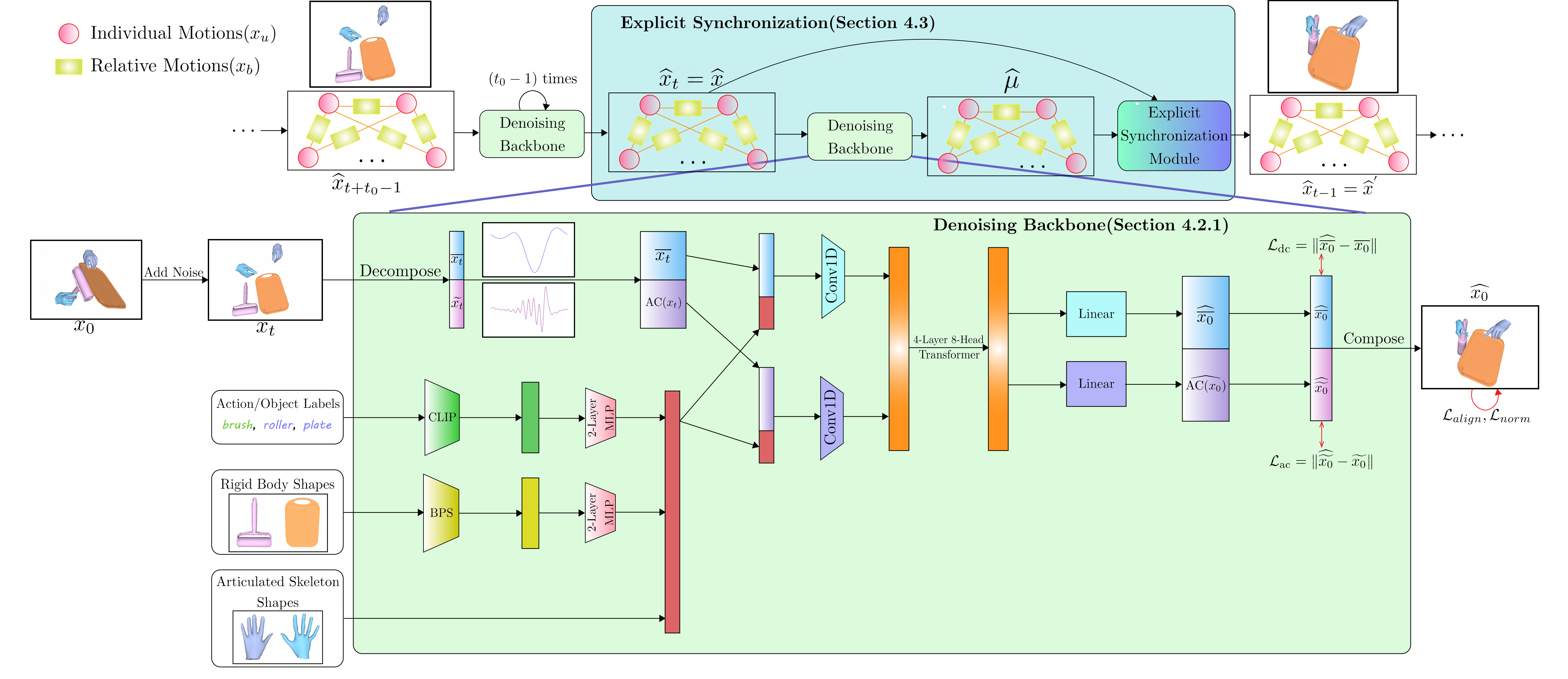
Figure 1: Overview of SyncDiff. The light blue box shows the inference process with explicit synchronization performed every $t_{0}$ step. For denoising steps irrelevant to explicit synchronization, the noise level is set to $\sigma_{t}$. For the calculation from $\hat{x}$ to $\hat{\mu}$, no noise is added. For the denoising process that involves explicit synchronization, the noise level is $\sigma_{t}^{{}^{\prime}}$. Please refer to Section 4.3 for more details. The light green box illustrates denoising model architecture (Section 4.2.1).

4.1 Factorized Motion Representations

1. Individual and Relative representations. For a single body $\textbf{b}=h_{i\in[1,n]}$ or $\textbf{b}=o_{j\in[1,m]}$, we represent its motion as $x_{u,\textbf{b}}$ in the world coordinate system. Here $x_{u,h_{i}}\in\mathbb{R}^{T\times D\times 3}$, where $D$ is the number of its joints, represents 3D joint positions. $x_{u,o_{j}}=[t_{j},q_{j}]\in\mathbb{R}^{T\times 7}$, where $t_{j}\in\mathbb{R}^{T\times 3}$ is its translation, and $q_{j}\in\mathbb{R}^{T\times 4}$ is the quaternion representing its orientation.

For two bodies $\textbf{b}_{1}$ and $\textbf{b}_{2}$, we use $x_{b,\textbf{b}_{2}\rightarrow\textbf{b}_{1}}$ to denote the relative motion of $\textbf{b}_{2}$ in $\textbf{b}_{1}$’s coordinate system. We require that $\textbf{b}_{1}$ is a rigid body, and omit relative representation between articulated skeletons. If $\textbf{b}_{2}$ is also a rigid body, then $x_{b,\textbf{b}_{2}\rightarrow\textbf{b}_{1}}=[t_{\textbf{b}_{2}\rightarrow\textbf{b}_{1}},q_{\textbf{b}_{2}\rightarrow\textbf{b}_{1}}]$, where $t_{\textbf{b}_{2}\rightarrow\textbf{b}_{1}}=q_{\textbf{b}_{1}}^{-1}(t_{\textbf{b}_{2}}-t_{\textbf{b}_{1}})$, and $q_{\textbf{b}_{2}\rightarrow\textbf{b}_{1}}=q_{\textbf{b}_{1}}^{-1}q_{\textbf{b}_{2}}$. If $\textbf{b}_{2}$ is an articulated skeleton, the position of one of its joints $p$ under individual representation will become $p^{{}^{\prime}}$ in $\textbf{b}_{1}$’s coordinate system, where $p^{{}^{\prime}}=q_{\textbf{b}_{1}}^{-1}(p-t_{\textbf{b}_{1}})$.

After deriving all individual and relative motion representations, we concatenate all of them into $x=[x_{u,o_{1}},x_{u,o_{2}},\dots,x_{u,o_{m}},x_{u,h_{1}},x_{u,h_{2}},\dots,x_{u,h_{n}},\\ x_{b,o_{2}\rightarrow o_{1}},x_{b,o_{3}\rightarrow o_{1}},\dots,x_{b,o_{m}\rightarrow o_{m-1}},x_{b,h_{1}\rightarrow o_{1}},x_{b,h_{1}\rightarrow o_{2}},\\ \dots,x_{b,h_{n}\rightarrow o_{m}}]\in\mathbb{R}^{T\times D_{\text{sum}}}$, where $D_{\text{sum}}=7m+3Dn+7{m\choose 2}+3Dmn$. Although $x$ is composed of individual and relative representations, for final synthesized motions of bodies, they only involve individual motions, and those relative ones serve merely as auxiliary components.

2. Motion Decomposition based on Frequency. For a motion sequence $x\in\mathbb{R}^{T\times D_{\text{sum}}}$, we select $T$ frequency bases $\phi_{l\in[0,T-1]}$=$\frac{l}{T}$, and then decompose $x$ into components of $\phi$:

$$x_{k\in[0,T-1]}=\sum\limits_{l=0}^{T-1}a_{l}\cos(k\phi_{l})+b_{l}\sin(k\phi_{l}),$$ (1)

where $a_{l},b_{l}\in\mathbb{R}^{D_{\text{sum}}}$ are the coefficients computed by Fast Fourier Transform (FFT). To prevent networks from overfitting high-frequency noises in mocap datasets, we select a frequency boundary $L\in[4,\frac{T}{4})$, and directly discard signals with frequencies higher than $L$. We then divide the remaining signals into direct currents ($\bar{x}$) and alternating currents ($\tilde{x}$) based on frequency:

$$\begin{split}&\bar{x}_{k}=\sum\limits_{l=-3}^{2}a_{l}\cos(k\phi_{l})+b_{l}\sin(k\phi_{l}),\text{ and}\\ &\tilde{x}_{k}=\sum\limits_{l\in[-L,-4]\cup[3,L-1]}a_{l}\cos(k\phi_{l})+b_{l}\sin(k\phi_{l}),\end{split}$$ (2)

where $a_{l}$=$a_{l+T}$ and $b_{l}$=$b_{l+T}$ for $l\in[-T,-1]$. Note that $\bar{x},\tilde{x}\in\mathbb{R}^{T\times D_{\text{sum}}}$. Additionally, We represent AC($x$) as $[a_{3},\\ \dots,a_{L-1},a_{T-L},$ $\dots,a_{T-4},b_{3},\dots,b_{L-1},b_{T-L},\dots,b_{T-4},\\ z]\in\mathbb{R}^{T\times D_{\text{sum}}}$, where $z$ is a zero matrix for filling AC($x$) to length $T$. Our model denoises on $\bar{x}$ and AC($x$), and measures the differences on $\bar{x}$ and $\tilde{x}$ between generated and ground-truth values in the temporal domain as supervision.

4.2 Implicit Joint Modeling

We use one single diffusion model (Figure 1) to jointly model all individual and relative motions. The introduction will be carried out from two aspects: basic model backbone (Section 4.2.1), and loss functions corresponding to our derived scores (Section 4.2.2).

4.2.1 Model Backbone

We adopt the latent diffusion [64] paradigm.

For action/object label features, unlike DiffH2O [13], which uses fully descriptive sentence annotations of data in GRAB [77], we do not assume that the given action labels and object labels can be efficiently and accurately concatenated into sentences, in order to improve the universality of our approach. Instead, we use pretrained CLIP [61] to extract features for each label individually (Specifically, the action label is expanded into the form of “A video of [action]”.), and process these features through an independent 2-layer MLP.

Following works like  [39, 40], object geometry features are encoded by BPS [57]. They then pass through an independent 2-layer MLP.

Concatenating the processed action/object label features, object geometry features, and shape parameters $\beta_{i\in[1,n]}$ together, we finally obtain the condition vector. This condition vector is replicated and combined with $\bar{x}$ and AC($x$) derived from noised $x$ respectively and passed through two separate convolutional layers into the latent space, and then concatenated to be denoised by a 4-layer, 8-head transformer. The denoised latent vectors are split and recovered with linear projectors as $\widehat{\overline{x_{0}}}$ and $\widehat{\text{AC}(x_{0})}$, the latter of which is reconstructed as $\widehat{\widetilde{x_{0}}}$. The final denoised motion sequence is recomposed by $\widehat{x_{0}}=\widehat{\overline{x_{0}}}+\widehat{\widetilde{x_{0}}}$.

4.2.2 Loss Functions

Suppose we need to supervise the final synthesis results $\{\hat{\bar{x}},\hat{\tilde{x}}\}$, where $\{\bar{x},\tilde{x}\}$ are ground-truth motions. Define $\hat{x}=\hat{\bar{x}}+\hat{\tilde{x}}$. We need loss functions corresponding to both the data sample and alignment scores.

For data sample scores, our method is similar to the standard reconstruction loss, except that we supervise $\bar{x}$ and $\tilde{x}$ separately. We denote $\mathcal{L}_{\text{dc}}=\|\hat{\bar{x}}-\bar{x}\|_{2}^{2}$, $\mathcal{L}_{\text{ac}}=\|\hat{\tilde{x}}-\tilde{x}\|_{2}^{2}$ and $\mathcal{L}_{\text{norm}}=\sum\limits_{j=1}^{m}\|1-|\hat{q}_{j}|\|_{2}^{2}$. The last one is used to induce the norms of the quaternions representing rigid body rotations to be as close to $1$, where $\hat{x}_{u,o_{j}}=[\hat{t}_{j},\hat{q}_{j}]$.

As for our alignment scores for pairwise bodies, we can similarly derive the alignment loss

$$\mathcal{L}_{\text{align}}= \sum\limits_{1\leq j_{1}<j_{2}\leq m}2\|\hat{x}_{b,o_{j_{2}}\rightarrow o_{j_{1}}}-\text{rel}(\hat{x}_{u,o_{j_{1}}},\hat{x}_{u,o_{j_{2}}})\|_{2}^{2}$$ (3)

$$+\sum\limits_{i\in[1,n],j\in[1,m]}\|\hat{x}_{b,h_{i}\rightarrow o_{j}}-\text{rel}(\hat{x}_{u,o_{j}},\hat{x}_{u,h_{i}})\|_{2}^{2},$$

where $\text{rel}(a,b)$ denotes $b$’s motion in $a$’s coordinate system.

Finally, the total loss function is calculated as:

$$\mathcal{L}=\lambda_{\text{dc}}\mathcal{L}_{\text{dc}}+\lambda_{\text{ac}}\mathcal{L}_{\text{ac}}+\lambda_{\text{align}}\mathcal{L}_{\text{align}}+\lambda_{\text{norm}}\mathcal{L}_{\text{norm}}.$$ (4)

Proof details of the formula and hyper-parameters are provided in the supplementary material.

4.3 Explicit Synchronization in Inference Time

Experiments show that after splitting the motion into $\bar{x}$ and $\tilde{x}$ for separate supervision, the issue of hand-object or human-object misalignment becomes more severe compared to simply using the mixed representation of $x=\bar{x}+\tilde{x}$. What’s worse, relying solely on implicit joint modeling cannot fully mitigate this issue. Our strategy is to introduce an explicit synchronization process during inference time, aiming to leverage both data sample scores and alignment scores to address this problem. Since the synchronization step is time-consuming, to balance performance and efficiency, we perform synchronization operations every $t_{0}(t_{0}<<\mathcal{T})$ steps, where $\mathcal{T}$ is the total number of denoising steps, as is shown in Figure 1. In particular, for each synchronization step at inference time, let the current predicted motion be $\hat{x}_{t}$. According to the diffusion formula [28], without synchronization, the next step would be:

$$\hat{x}_{t-1}=\hat{\mu}(\hat{x}_{t},t)+\sigma_{t}\epsilon(\epsilon\sim\mathcal{N}(0,I)),$$ (5)

where $\hat{\mu}$ is the predicted mean value, and $\sigma_{t}$ is a predefined constant real number. For convenience, we denote the motion before synchronization as $\hat{x}$ and the motion after synchronization as $\hat{x}^{{}^{\prime}}$. Let $\sigma_{t}$ be abbreviated as $\sigma$. For different parts of $\hat{x}^{{}^{\prime}}$, we handle them as follows:

1. Individual Motions of Rigid Bodies. Let

$$\begin{split}\hat{x}_{u,o_{j}}^{{}^{\prime}}=&\frac{\frac{2}{m-1}\sigma^{2}\overline{\lambda}}{1+2\sigma^{2}\overline{\lambda}}\sum\limits_{j^{{}^{\prime}}\neq j}\text{comb}\left(\hat{x}_{u,o_{j^{{}^{\prime}}}},\hat{x}_{b,o_{j}\rightarrow o_{j^{{}^{\prime}}}}\right)\\ &+\frac{1}{1+2\sigma^{2}\overline{\lambda}}\hat{\mu}_{u,o_{j}}+\sigma^{{}^{\prime}}\epsilon,\end{split}$$ (6)

where $\text{comb}\left(\hat{x}_{u,o_{j^{{}^{\prime}}}},\hat{x}_{b,o_{j}\rightarrow o_{j^{{}^{\prime}}}}\right)$ utilizes the individual representation of $o_{j^{{}^{\prime}}}$ and relative representation between $o_{j^{{}^{\prime}}}$ and $o_{j}$ to compute coordinates of $o_{j}$. Note that if $j^{{}^{\prime}}>j$, $\hat{x}_{b,o_{j}\rightarrow o_{j^{{}^{\prime}}}}$ is actually $\hat{x}_{b,o_{j^{{}^{\prime}}}\rightarrow o_{j}}$. $\overline{\lambda}=\frac{\lambda_{\text{exp}}}{\mathcal{R}}\sum\limits_{r=1}^{\mathcal{R}}\frac{1}{2\sigma_{i_{r}}^{2}}$, where $1\leq i_{1}<i_{2}<\dots<i_{\mathcal{R}}\leq\mathcal{T}$ are the synchronization timesteps, and $\sigma_{i_{1}}$, $\sigma_{i_{2}}$, $\dots$, $\sigma_{i_{\mathcal{R}}}$ are the original correspondent standard variances(without synchronization). Finally, $\sigma^{{}^{\prime}}=\sqrt{\frac{\sigma^{2}}{1+2\sigma^{2}\overline{\lambda}}}$. Specifically, when $m=1$, we do not perform synchronization for this part, and the denoising formula is identical to that without synchronization.

2. Individual Motions of Articulated Skeletons. Let

$$\begin{split}\hat{x}_{u,h_{i}}^{{}^{\prime}}=&\frac{\frac{2}{m}\sigma^{2}\overline{\lambda}}{1+2\sigma^{2}\overline{\lambda}}\sum\limits_{j\in[1,m]}\text{comb}\left(\hat{x}_{u,o_{j}},\hat{x}_{b,h_{i}\rightarrow o_{j}}\right)\\ &+\frac{1}{1+2\sigma^{2}\overline{\lambda}}\hat{\mu}_{u,h_{i}}+\sigma^{{}^{\prime}}\epsilon,\end{split}$$ (7)

Definitions of $\overline{\lambda}$ and $\sigma^{{}^{\prime}}$ are the same as Eq. 6.

3. Relative Motions. Let

$$\hat{x}_{b,{o_{j}\rightarrow o_{j^{{}^{\prime}}}}}^{{}^{\prime}}=\frac{1}{1+2\sigma^{2}\overline{\lambda}}\hat{\mu}_{b,{o_{j}\rightarrow o_{j^{{}^{\prime}}}}}+\frac{2\sigma^{2}\overline{\lambda}}{1+2\sigma^{2}\overline{\lambda}}\text{rel}\left(\hat{x}_{u,o_{j^{{}^{\prime}}}},\hat{x}_{u,o_{j}}\right)+\sigma^{{}^{\prime}}\epsilon,$$

$$\hat{x}_{b,h_{i}\rightarrow o_{j}}^{{}^{\prime}}=\frac{1}{1+2\sigma^{2}\overline{\lambda}}\hat{\mu}_{b,h_{i}\rightarrow o_{j}}+\frac{2\sigma^{2}\overline{\lambda}}{1+2\sigma^{2}\overline{\lambda}}\text{rel}\left(\hat{x}_{u,o_{j}},\hat{x}_{u,h_{i}}\right)+\sigma^{{}^{\prime}}\epsilon.$$

Definitions of $\overline{\lambda}$ and $\sigma^{{}^{\prime}}$ are the same as Eq. 6.

After synchronization operations and deriving $\hat{x}^{{}^{\prime}}$, it is again used for further denoising. Between two adjacent synchronization steps, we still directly use Eq. 5 for stepwise denoising, and do not perform synchronization operations. We demonstrate in supplementary materials, that the above equations are equivalent to maximum likelihood sampling from the newly computed Gaussian distribution based on both data sample scores and alignment scores.

4.4 Post Process: Mesh Reconstruction

For tasks such as robot learning, having only the joints is sufficient; however, for tasks like animation production, it is necessary to reconstruct the full meshes. In this section, we introduce how to reconstruct hand mesh or human body mesh of natural shape from the predicted joint positions $\mathbb{R}^{T\times D\times 3}$.

Hand Mesh Reconstruction. For one single hand, suppose the predicted joint positions are $\hat{x}\in\mathbb{R}^{T\times 21\times 3}$. We start with tunable MANO [65] parameters for joint pose $\theta\in\mathbb{R}^{T\times 45}$, global orientation $R\in\mathbb{R}^{T\times 3}$ and translation $l\in\mathbb{R}^{T\times 3}$, which are all set to zero tensors. We freeze hand shape $\beta\in\mathbb{R}^{10}$. During the optimizing process, let the current calculated joint positions be $K\in\mathbb{R}^{T\times 21\times 3}$ based on $\theta$, $R$, and $l$. We want to minimize

$$\mathcal{L}_{\text{MANO}}=\lambda_{\text{pos}}\mathcal{L}_{\text{pos}}+\lambda_{\text{angle}}\mathcal{L}_{\text{angle}}+\lambda_{\text{vel}}\mathcal{L}_{\text{vel}}$$

Here

$$\mathcal{L}_{\text{pos}}=\sum\limits_{t=1}^{T}\sum\limits_{i=1}^{21}\|\hat{x}_{t,i}-K_{t,i}\|_{2}^{2}$$

which minimizes the difference between joint positions $K$ from MANO calculation and our predicted results $\hat{x}$.

$$\mathcal{L}_{\text{angle}}=\sum\limits_{t=1}^{T}\sum\limits_{i=1}^{45}[\max(\theta_{t,i}-u_{i},0)+\max(d_{i}-\theta_{t,i},0)]$$

where $(d_{i},u_{i})$ is the permitted rotation range for the $i$-th degree of freedom. This loss item ensures that the rotation angle of each joint remains within permittable limits, preventing unreasonable distortions.

$$\mathcal{L}_{\text{vel}}=\sum\limits_{t=1}^{T-1}\|l_{t}-l_{t+1}\|_{2}^{2}$$

which keeps the positions at adjacent time steps close to ensure a smooth trajectory without abrupt changes.

Human Body Mesh Reconstruction. Similar to MANO in hand pose representation, for human body pose representation, we also have SMPL-X [55] representation. It is composed of a set of parameters $(\theta,R,l,\theta_{\text{left}},\theta_{\text{right}})$, where the body pose $\theta\in\mathbb{R}^{T\times 21\times 3}$ represents the $21$ joint orientations(except root), $R,l\in\mathbb{R}^{T\times 3}$ are global orientation and translation, and $\theta_{\text{left}},\theta_{\text{right}}\in\mathbb{R}^{T\times 12}$ are compressed representations of two hands. Human shape parameters $\beta\in\mathbb{R}^{10}$ are given, while $\hat{x}\in\mathbb{R}^{T\times 22\times 3}$ denotes the joint positions we predict.

Due to the flexibility of human body poses, to reconstruct the human body mesh, we not only need joint positions but also joint orientations. Therefore, we need to introduce additional $T\times 21\times 3$ degrees of freedom to every $x_{u,h_{i}}(i\in[1,n])$, representing the predicted human body pose $\hat{\theta}$ under SMPL-X. These degrees of freedom are also predicted by the diffusion model, but they only participate in the decomposition process and do not get involved in our two synchronization mechanisms.

Similar to hand mesh reconstruction, we start with tunable SMPL-X parameters $R,l,\theta_{\text{left}},\theta_{\text{right}}$, which are all set to zero tensors. We freeze hand shape $\beta\in\mathbb{R}^{10}$ and $\theta=\hat{\theta}$. During the optimizing process, let the current calculated joint positions be $K\in\mathbb{R}^{T\times 22\times 3}$ based on $R,l,\theta_{\text{left}},\theta_{\text{right}}$. We want to minimize

$$\mathcal{L}_{\text{SMPL-X}}=\lambda_{\text{pos}}\mathcal{L}_{\text{pos}}+\lambda_{\text{vel}}\mathcal{L}_{\text{vel}}$$

Here

$$\mathcal{L}_{\text{pos}}=\sum\limits_{t=1}^{T}\sum\limits_{i=1}^{22}\|\hat{x}_{t,i}-K_{t,i}\|_{2}^{2}$$

which minimizes the difference between joint positions from SMPL-X calculation and our predicted results.

$$\mathcal{L}_{\text{vel}}=\sum\limits_{t=1}^{T-1}\|l_{t}-l_{t+1}\|_{2}^{2}$$

which keeps the trajectory smooth.

The hyperparameters involved in the mesh reconstruction process can be found in Table  11 and  12.

5 Experiments

5.1 Datasets

To examine our method’s generalizability across various multi-body interaction configurations, we utilize four datasets with different interaction scenarios: TACO [46] (two hands and two objects), CORE4D [100] (two people and one object), GRAB [77] (one or two hands and one object), and OAKINK2 [99] (two hands and one to three objects). We describe data splits for each dataset below.

(1) TACO: We use the official split of TACO, with four testing sets, each representing different scenarios: 1) the interaction triplet $\langle$action, tool category, target object category$\rangle$ and the object geometries are all seen in the training set, 2) unseen object geometry, 3) unseen triplet, and 4) unseen object category and geometry.

(2) CORE4D: We divide $875$ motion sequences into one training set and two testing sets, where the two testing sets represent seen and unseen object geometries, respectively. The $\langle$action, object category$\rangle$ pairs from testing sets are all involved in the training set.

(3) GRAB: We use an existing data split of unseen subjects from IMoS [22] and that of unseen objects from DiffH2O [13]. Please refer to the two papers for details.

(4) OAKINK2: We utilize the train, val, and test divisions stated in the TaMF task of their paper.

Toward a fair comparison with DiffH2O [13], we follow the setting of DiffH2O for GRAB, where methods are required to generate hand-object manipulations after grasping objects. For the other three datasets, all methods need to synthesize complete multi-body interaction motion sequences without direct guidance.

5.2 Evaluation Metrics

To evaluate the qualities of synthesized motion sequences comprehensively, we present two types of evaluation metrics focusing on fine-grained physical plausibility and general motion semantics, respectively.

(1) Physics-based metrics measure the physical plausibility of hand-object/human-object interactions and the extent of motion coordination among different bodies. We use the Contact Surface Ratio (CSR) for hand-object settings and the Contact Root Ratio (CRR) for human-object settings to denote the proportion of motion sequences where hand-object/human-object contact occurs. Contact is defined as the hand mesh being within $5$mm of at least one object for CSR, and the two hand roots of a human consistently being within $3$cm of at least one object for CRR. When there are multiple hands or humans, we take the average among all of them. We label the frames based on whether hand-object contact occurs for ground-truth and synthesized motions and then compute their Intersection-over-Union (IoU), denoted as CSIoU. Besides, Interpenetration Volume (IV) and Interpenetration Depth (ID) are incorporated to assess penetration between different bodies.

(2) Motion semantics metrics evaluate high-level motion semantics and its distributions, comprising Recognition Accuracy (RA), Fréchet Inception Distance (FID), Sample Diversity (SD), and Overall Diversity (OD). Following existing evaluations for motion synthesis [40, 39], we train a network to extract motion features and predict action labels using ground-truth motion data. For better feature semantics, the network is trained on the combination of all train, val, and test splits. RA denotes the action recognition accuracy of the network on synthesized motions. FID measures the difference in feature distributions of generated and ground-truth motions. Following  [13], SD represents the mean Euclidean distance between multiple generated wrist trajectories in a single sample, and OD refers to the mean distance between all generated trajectories in a dataset split.

5.3 Comparison to Existing Methods

	CSIoU (%, $\uparrow$)				IV ($\text{cm}^{3}$, $\downarrow$)				FID ($\downarrow$)				RA (%, $\uparrow$)
Method	Test1	Test2	Test3	Test4	Test1	Test2	Test3	Test4	Test1	Test2	Test3	Test4	Test1	Test2	Test3	Test4
Ground-truth	100.0	100.0	100.0	100.0	4.56	3.60	4.24	3.50	0.03	0.03	0.03	0.04	84.92	89.00	75.86	65.90
MACS [69]	56.81	53.79	21.38	12.09	13.18	18.57	10.33	8.99	10.56	23.24	32.18	42.37	58.40	53.08	33.00	19.02
DiffH2O [13]	62.29	46.38	42.12	16.38	10.25	15.21	4.67	5.70	4.34	17.04	24.92	39.20	61.40	56.70	43.67	28.15
Ours	73.00	70.94	43.22	26.70	6.64	3.81	4.02	7.73	2.70	2.68	22.96	30.23	73.28	85.92	46.90	40.12
w/o all	62.96	52.38	38.02	26.39	7.95	12.02	7.05	7.67	10.63	21.87	30.17	46.38	57.39	48.05	37.13	24.92
w/o decompose	68.86	54.77	41.70	28.07	6.80	10.78	6.93	7.22	6.44	21.21	28.67	49.58	56.60	51.85	40.02	22.18
w/o $\mathcal{L}_{\text{align}}$, exp sync	63.74	48.35	39.89	20.87	14.28	13.80	5.93	7.44	4.13	4.32	24.65	38.73	64.47	62.12	41.68	30.39
w/o $\mathcal{L}_{\text{align}}$	70.39	67.15	40.38	26.83	6.29	4.86	5.88	7.39	2.90	3.02	22.28	32.78	67.82	79.30	44.75	34.51
w/o exp sync	65.51	50.33	37.72	23.61	13.08	14.40	6.20	7.75	3.39	3.30	21.26	33.67	67.27	78.50	45.82	37.13

Table 1: Results on TACO [46] dataset. The best in each column is highlighted in bold.

Hand-Object Interaction. For hand-object interaction motion synthesis, we compare our SyncDiff to two state-of-the-art approaches MACS [69] and DiffH2O [13]. For MACS, we first generate the motions of all objects in their object trajectory synthesis phase, and then directly use their hand motion synthesis phase to get overall results. For DiffH2O, we use the version without grasp reference input.

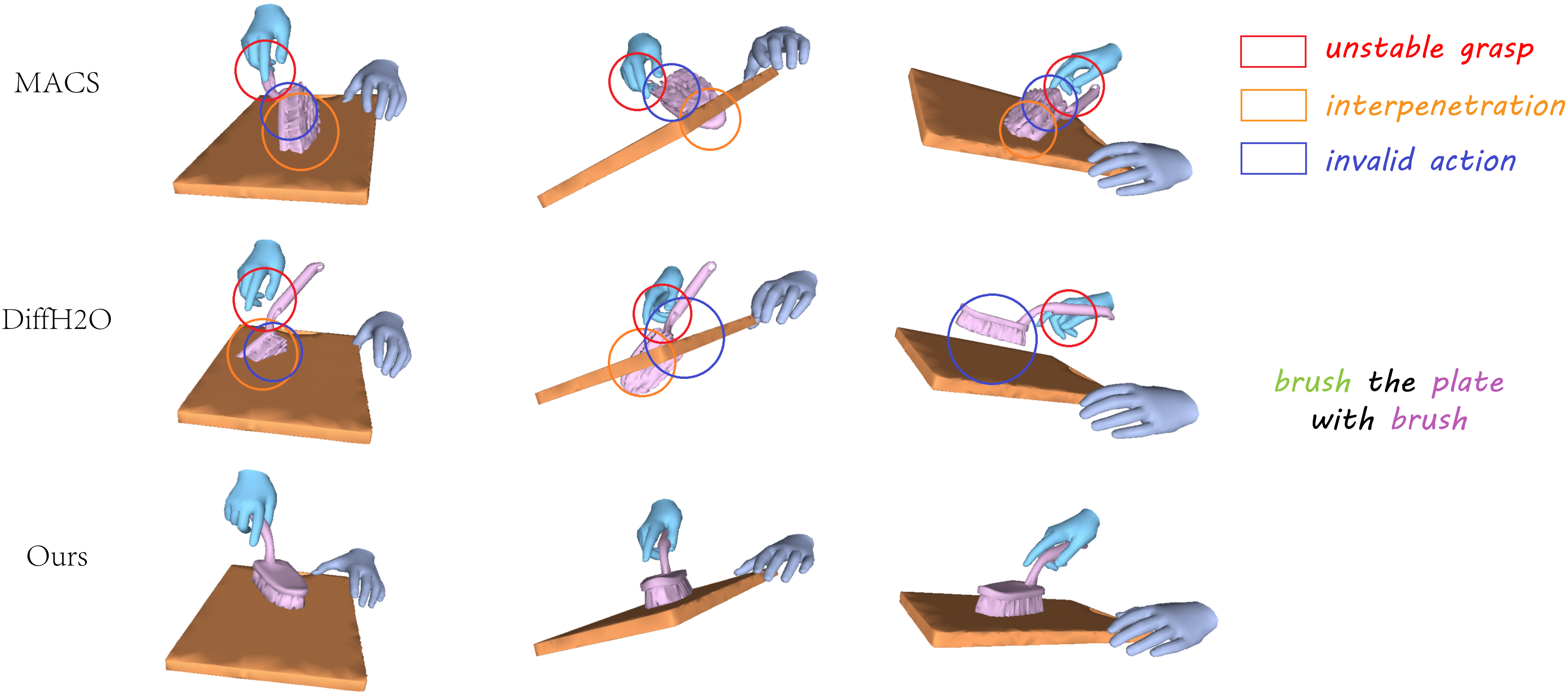
Figure 2: Qualitative results from TACO [46] dataset. Invalid action indicates the poses cannot complete the operation effectively.

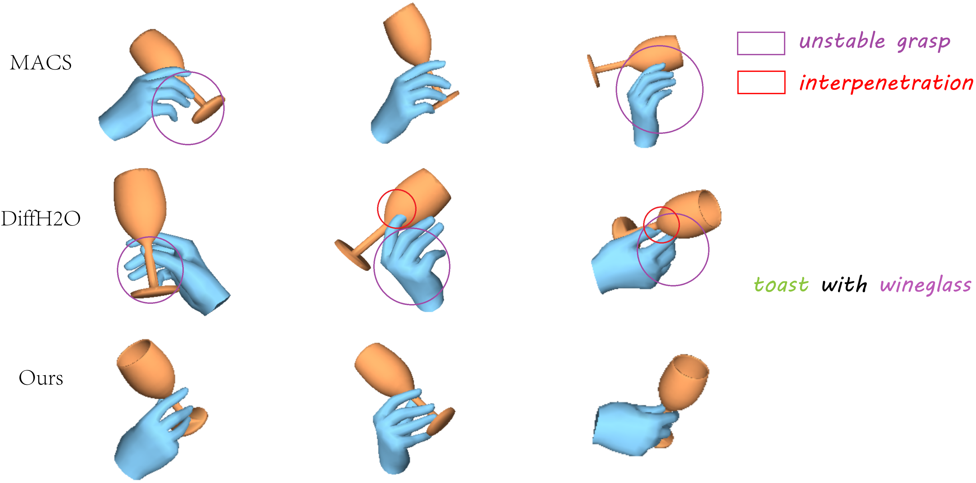
Figure 3: Qualitative results from GRAB [77] dataset.

As is shown in Table 1, 2, and 4, our method outperforms MACS and DiffH2O by a large margin with better CSIoU, CSR, IV, and ID. The reason is that our method features more robust alignment and synchronization mechanisms to ensure synchronization which are excluded in existing methods. Figure 2 compares results from different methods qualitatively. In the results from MACS and DiffH2O, the brush often penetrates the plate, and the pose of the brush does not guarantee the bristles being pressed closely against the plate, effectively completing the action. FID and RA further indicate that the motions generated by our method are more realistic. This is still caused by the more precise generation quality of object-object interactions from our method, and our separation of motions at different frequencies ensures that subtle high-frequency periodic movements are not overshadowed, which are crucial for identifying action types. Figure 4 demonstrates the benefits of our synchronization mechanism. Although MACS uses relative representations for some hand-object pairs to ensure firm grasp, due to the lack of synchronization on the complete graphical model, conflicts arise between the left hand and the knife, which should not directly interact. Figure 6 indicates that with a higher demand for coordination quality among objects, our method can also address hand-object and object-object synchronization effectively.

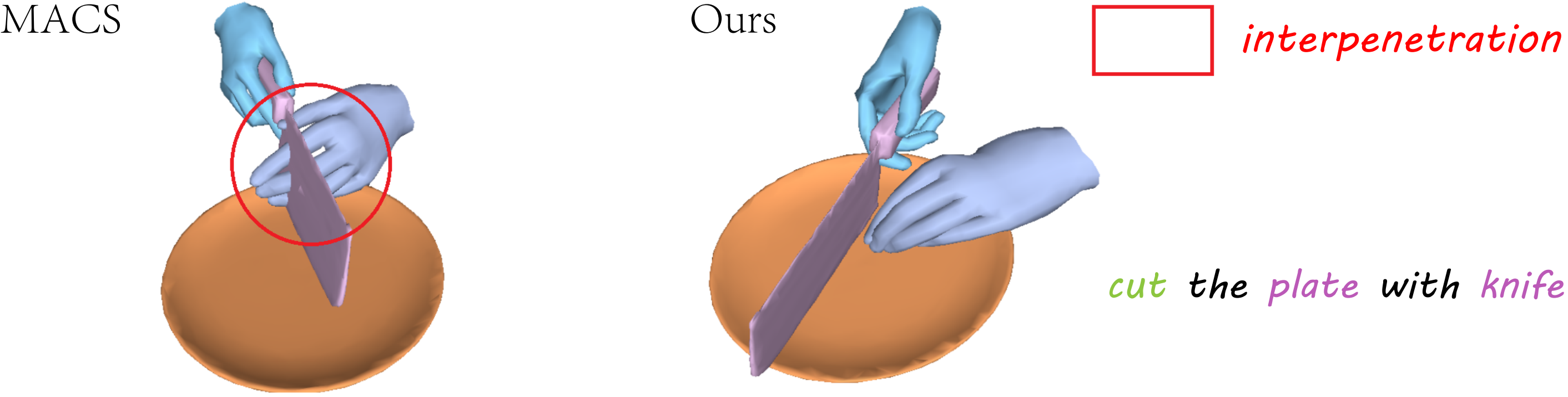
Figure 4: Qualitative results from TACO [46] dataset.

Human-Object Interaction. For human-object interaction synthesis, we compare our method to ComMDM [68], InterGen [42], and OMOMO [40]. ComMDM and InterGen are capable of generating interactions between two people. For OMOMO, we first use their conditional diffusion models to generate object trajectories, and then use their whole pipeline to synthesize complete Multi-body HOI motion.

As shown in Table 3 and Figure 5, our method outperforms all three baseline methods in physics-based and semantics metrics and obtains the most realistic qualities. Generated motions from existing methods suffer from unnatural grasping poses and arm-object interpenetration, while our method mitigates these issues.

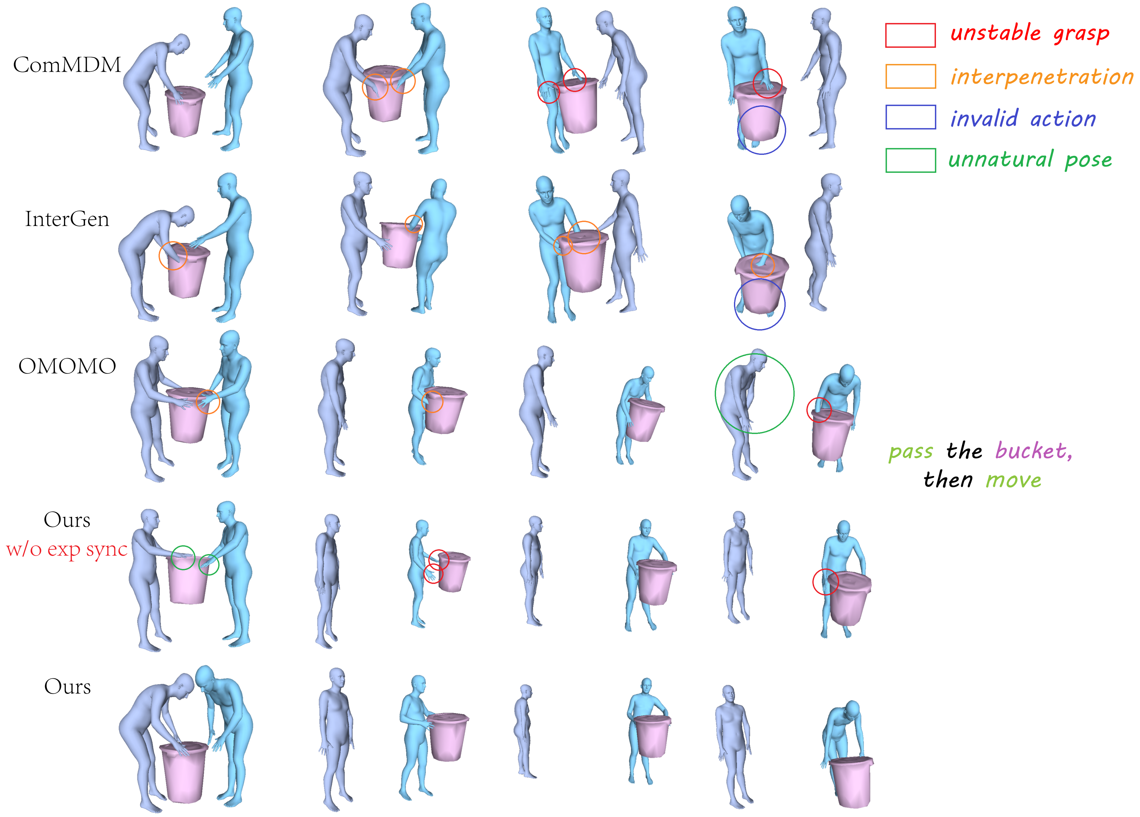
Figure 5: Qualitative comparisons on CORE4D [100] dataset.

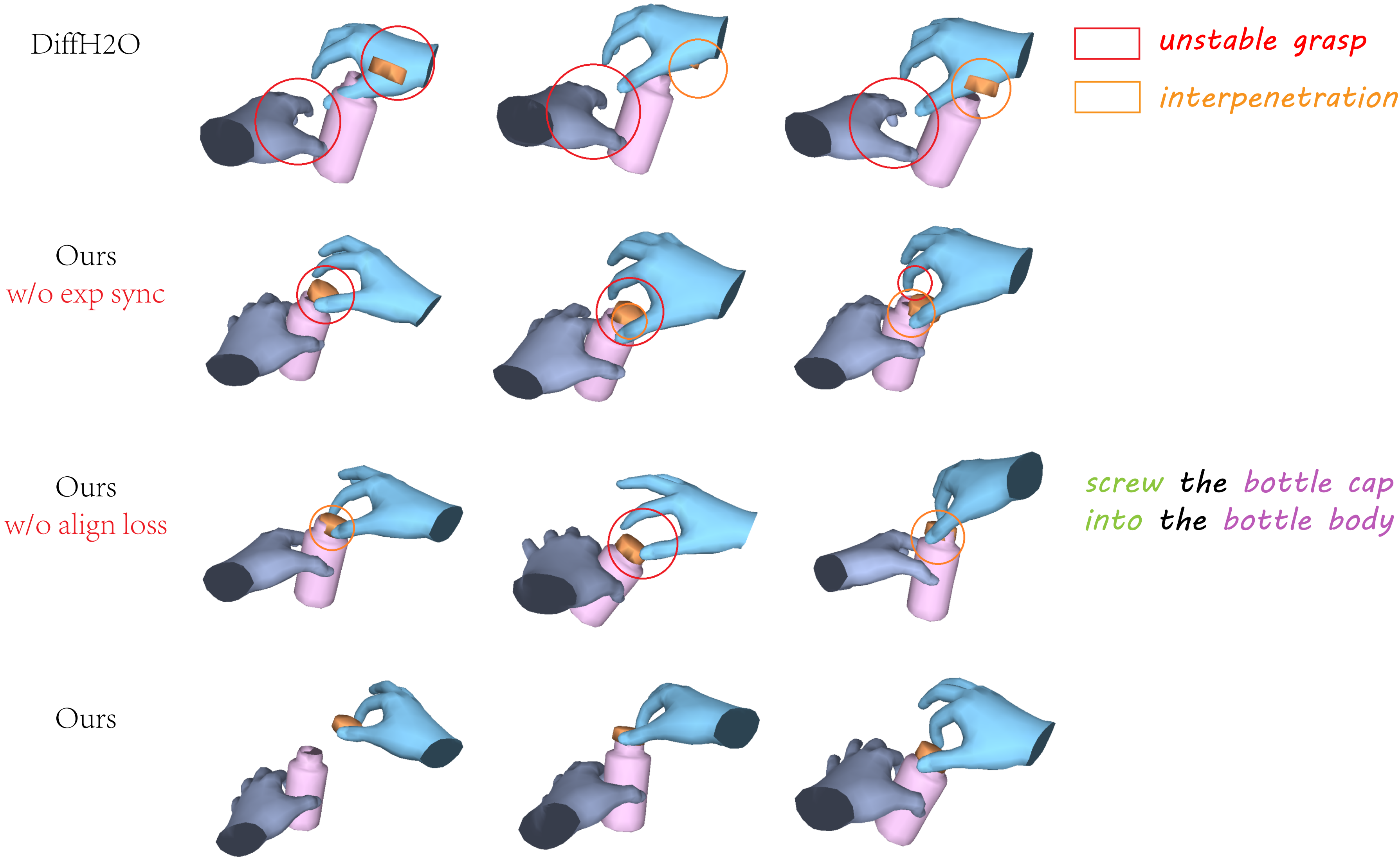
Figure 6: Qualitative results on OAKINK2 [99] dataset. The task requires precise contact between objects, where the bottle cap needs to align perfectly with the bottle, and there needs to be a tendency for it to be twisted down in a clockwise spiral.

	Method	Backbone	SD ($\text{m},\uparrow$)	OD ($\text{m},\uparrow$)	IV ($\text{cm}^{3},\downarrow$)	ID ($\text{mm},\downarrow$)	CSR ($\%,\uparrow$)	Hand Motion RA ($\%,\uparrow$)	Hand-Object Motion RA ($\%,\uparrow$)
Unseen subject split	IMoS [22]	CVAE	0.002	0.149	7.14	11.47	5.0	57.9	58.8
	DiffH2O [13]	Transformer	0.088	0.185	6.65	8.39	6.7	76.0	81.0
	DiffH2O [13]	UNet	0.109	0.188	6.02	7.92	6.4	83.3	87.5
	MACS [69]	MLP+Conv	0.059	0.164	8.29	10.12	3.9	72.9	76.4
	Ours	Transformer	0.106	0.188	6.22	7.75	7.2	82.6	88.9
Unseen object split	IMoS [22]	CVAE	0.002	0.132	10.38	12.45	4.8	56.1	58.1
	DiffH2O [13]	Transformer	0.133	0.185	7.99	10.87	7.3	75.0	80.3
	DiffH2O [13]	UNet	0.134	0.179	9.03	11.39	8.6	75.5	83.7
	MACS [69]	MLP+Conv	0.105	0.156	11.24	13.42	5.4	57.7	63.9
	Ours	Transformer	0.148	0.192	7.07	10.67	10.5	77.4	86.5

Table 2: Comparison on GRAB [77] dataset for the post-grasping phase. We conduct experiments on the post-grasping hand-object manipulation phase to compare with DiffH2O [13]. Each column highlights the best method in red, with the second best highlighted in blue. Results of IMoS [22] and DiffH2O are from the original paper of DiffH2O, while MACS [69] results are obtained via our re-implementation.

5.4 Ablation studies

We examine the effect of our three key designs (frequency-domain motion decomposition, the alignment loss $\mathcal{L}_{\text{align}}$, and the explicit synchronization) separately. The results after removing each of these three components individually are shown as “w/o decompose”, “w/o $\mathcal{L}_{\text{align}}$”, and “w/o exp sync”. Two additional ablations are to remove the two synchronization mechanisms and all three designs, denoted as “w/o $\mathcal{L}_{\text{align}}$, exp sync” and “w/o all”, respectively. Results in Table 1, 3, and 4 show that removing any of the above three components can lead to varying extents of performance decline. Compared to the method without any key design, simply incorporating frequency-domain decomposition obtains coherent performance drops under nearly all physics-based metrics due to more challenging multi-body synchronization. Nevertheless, the two synchronization strategies consistently enhance the effects and finally achieve the best results on nearly all evaluation aspects.

Removal of Decomposition. As shown in Figure 7, after removing the decomposition mechanism, once periodic relative motion is involved in the interactions between objects, It becomes easier for the motions to be overly smooth, which is intuitively manifested as two objects being in an almost relative stationary state, making it difficult to complete the action. This also results in poor performance in semantics metrics FID and RA from Table 1,  3, and  4.

	CRR(%, $\uparrow$)		FID($\downarrow$)		RA (%, $\uparrow$)
Method	Test1	Test2	Test1	Test2	Test1	Test2
Ground-truth	7.72	6.25	0.01	0.00	96.45	97.44
ComMDM [68]	4.65	4.38	17.03	20.56	53.30	49.74
InterGen [42]	4.92	4.54	15.10	17.60	69.54	60.00
OMOMO [40]	5.31	5.54	13.22	14.94	68.02	65.13
Ours	6.15	5.78	6.45	7.25	92.89	90.26
w/o all	5.42	5.35	17.21	21.37	54.82	48.72
w/o decompose	5.70	5.46	8.42	9.54	75.13	71.28
w/o $\mathcal{L}_{\text{align}}$, exp sync	4.84	4.88	7.43	8.49	82.74	74.11
w/o $\mathcal{L}_{\text{align}}$	5.38	5.25	6.74	8.31	90.36	87.69
w/o exp sync	5.23	5.04	7.55	7.89	80.20	78.46

Table 3: Results on CORE4D [100] dataset. The best in each column is highlighted in bold.

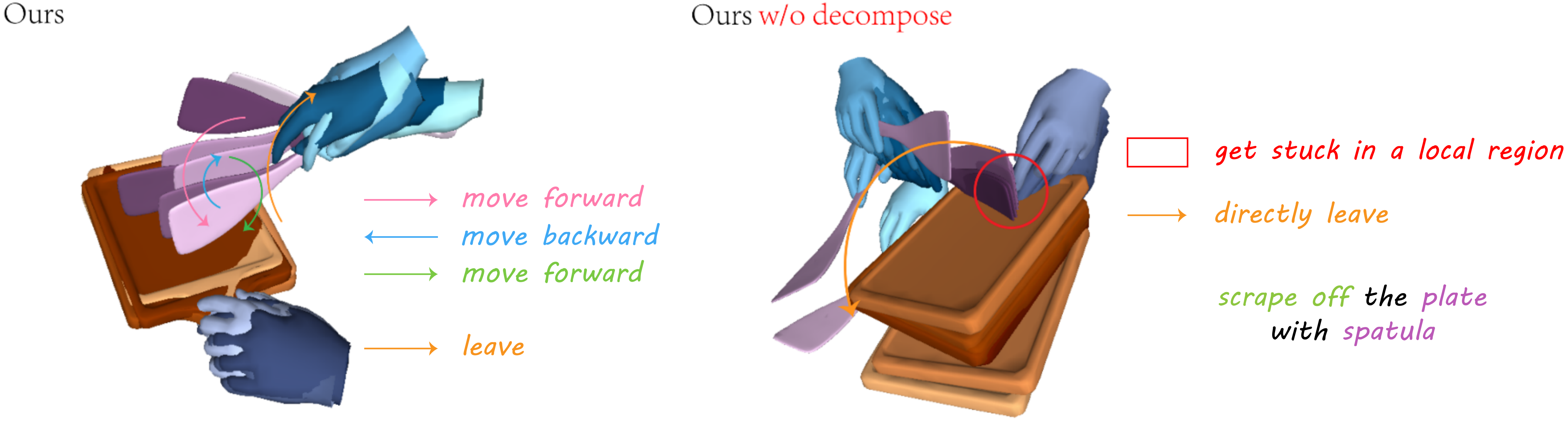
Figure 7: Qualitative results from TACO [46] dataset. Periodic relative motion is required between two objects. The color changes from deep to light, representing time passage. It can be observed that after removing the decomposition mechanism, the spatula tends to get stuck in a small area on the plate’s surface.

Method	CSIoU	IV	FID	RA
	(%, $\uparrow$)	($\text{cm}^{3}$, $\downarrow$)	($\downarrow$)	(%, $\uparrow$)
Ground-truth	100.0	2.51	0.00	82.57
MACS [69]	57.52	10.52	4.96	54.91
DiffH2O [13]	55.50	5.59	5.18	50.48
Ours	72.14	4.41	2.65	74.83
w/o all	62.96	6.73	6.63	48.96
w/o decompose	68.16	4.90	4.46	55.05
w/o $\mathcal{L}_{\text{align}}$, exp sync	57.59	8.94	3.82	70.54
w/o $\mathcal{L}_{\text{align}}$	67.44	5.34	3.76	70.82
w/o exp sync	58.05	7.66	3.58	69.16

Table 4: Results on OAKINK2 [99] dataset. The best in each column is highlighted in bold.

Removal of $\mathcal{L}_{\text{align}}$ or Explicit Synchronization. As is shown in Figure 5 and 6, removing either one of $\mathcal{L}_{\text{align}}$ or explicit synchronization leads to unreasonable penetration or contact loss between objects or between humans and objects, with explicit synchronization playing a more significant role. This phenomenon is also revealed in quantitative evaluation results from Table  1,  3 and  4.

6 Conclusions

We present SyncDiff, a universal framework for synchronized motion synthesis of multi-body HOI interaction by estimating both data sample scores and alignment scores, and jointly optimizing sample and alignment likelihoods in inference. We also introduce a frequency-domain decomposition to better capture high-frequency, small-amplitude motion details. Experiments on four datasets demonstrate that SyncDiff can be adapted to synthesize synchronized multi-body human-object interaction sequences with any number of humans, hands, and rigid objects. Comparative experiments also demonstrate that in each specific setting, our method achieves better physical accuracy and action semantics than a range of state-of-the-art works. Some limitations of our work and their potential solutions are discussed in the appendix.

Appendix

Appendix A Details of Our Two Synchronization Mechanisms

A.1 Diffusion Model Basics

Diffusion models [71] and its variants [74, 28], especially latent diffusion, have been widely applied in different tasks, such as high-resolution image generation [64] or video generation [30]. They simulate the data distribution by introducing a series of variables $\{x_{i}\}_{i=1}^{\mathcal{T}}$ with different noise levels. The forward noise process can be represented as

$$q(x_{t}|x_{t-1})=\mathcal{N}(x_{t};\sqrt{1-\beta_{t}}x_{t-1},\beta_{t}I),$$

where $0<\beta_{t}<1$. We can derive that

$$x_{t}=\sqrt{\bar{\alpha}_{t}}x_{0}+\sqrt{1-\bar{\alpha}_{t}}\epsilon,$$

where $\epsilon\sim\mathcal{N}(0,I)$, and $\bar{\alpha}_{t}=\prod_{i=1}^{t}(1-\beta_{i})$.

For the inference process, from $\mathcal{T}$ that is large enough so that $p(x_{\mathcal{T}})\approx\mathcal{N}(0,I)$, do reverse sampling step by step, following

$$p_{\theta}(x_{t-1}|x_{t})=\mathcal{N}(x_{t-1};\mu_{\theta}(x_{t},t),\sigma_{t}^{2}I),$$

where $\mu_{\theta}$ is the mean distribution center predicted by network, and $\sigma_{t}^{2}$ is pre-defined constant variance. Then

$$x_{t-1}=\mu_{\theta}(x_{t},t)+\sigma_{t}z(z\sim\mathcal{N}(0,I)).$$

Finally we can get $x_{0}$, which is the denoised sample.

A.2 Complete Proof of Our Two Synchronization Mechanisms

First let’s derive some commonly used formulas in diffusion models that we will need in our proof, which the readers might not be familiar with. If you are familiar with the step-by-step denoising formula of diffusion, you can skip directly to Eq  8 and  9.

Suppose the noise-adding process has a total of $T$ steps, with each step’s amplitude denoted by $\beta_{t}(t\in[T])$, we define $\alpha_{t}=1-\beta_{t}$, and $\bar{\alpha}_{t}=\prod_{t=1}^{T}\alpha_{t}$.

Then by basic principles of diffusion models, we have

$$x_{t}\sim\mathcal{N}(\sqrt{\alpha_{t}}x_{t-1},(1-\alpha_{t})I)$$

$$x_{t-1}\sim\mathcal{N}(\sqrt{\bar{\alpha}_{t-1}}x_{0},(1-\bar{\alpha}_{t-1})I)$$

$$x_{t}\sim\mathcal{N}(\sqrt{\bar{\alpha}_{t}}x_{0},(1-\bar{\alpha}_{t})I)$$

According to Bayesian’s Formula,

$$q(x_{t-1}|x_{t},x_{0})=\frac{q(x_{t}|x_{t-1})q(x_{t-1}|x_{0})}{q(x_{t}|x_{0})}$$

Taking negative logarithmic,

$$-\log q(x_{t-1}|x_{t},x_{0})$$

$$=\frac{(x_{t}-\sqrt{\alpha_{t}}x_{t-1})^{2}}{2(1-\alpha_{t})}+\frac{(x_{t-1}-\sqrt{\bar{\alpha}_{t-1}}x_{0})^{2}}{2(1-\bar{\alpha}_{t-1})}$$

$$-\frac{(x_{t}-\sqrt{\bar{\alpha}_{t}}x_{0})^{2}}{2(1-\bar{\alpha}_{t})}+\text{Const}$$

$$=\left[\frac{\alpha_{t}}{2(1-\alpha_{t})}+\frac{1}{2(1-\bar{\alpha}_{t-1})}\right]x_{t-1}^{2}$$

$$-2\left[\frac{\sqrt{\alpha}_{t}}{2(1-\alpha_{t})}x_{t}+\frac{\sqrt{\bar{\alpha}_{t-1}}}{2(1-\bar{\alpha}_{t-1})}x_{0}\right]x_{t-1}+C(x_{t},x_{0})$$

$$\overset{\triangle}{=}Ax_{t-1}^{2}+Bx_{t-1}+C$$

$$=A\left(x_{t-1}+\frac{B}{2A}\right)^{2}+C^{{}^{\prime}}$$

so

$$x_{t-1}\sim\mathcal{N}\left(-\frac{B}{2A},\frac{1}{2A}I\right)\overset{\triangle}{=}\mathcal{N}(\mu_{t},\sigma_{t}^{2}I)$$

where

$$\mu_{t}=-\frac{B}{2A}$$

$$=\frac{\frac{\sqrt{\alpha_{t}}}{{1-\alpha_{t}}}x_{t}+\frac{\sqrt{\bar{\alpha}_{t-1}}}{1-\bar{\alpha}_{t-1}}x_{0}}{\frac{\alpha_{t}}{1-\alpha_{t}}+\frac{1}{1-\bar{\alpha}_{t-1}}}$$

$$=\frac{\sqrt{\alpha}_{t}(1-\bar{\alpha}_{t-1})}{\alpha_{t}(1-\bar{\alpha}_{t-1})+1-\alpha_{t}}x_{t}+\frac{\sqrt{\bar{\alpha}_{t-1}}(1-\alpha_{t})}{\alpha_{t}(1-\bar{\alpha}_{t-1})+(1-\alpha_{t})}x_{0}$$

$$=\frac{\sqrt{\alpha}_{t}(1-\bar{\alpha}_{t-1})}{1-\bar{\alpha}_{t}}x_{t}+\frac{\sqrt{\bar{\alpha}_{t-1}}(1-\alpha_{t})}{1-\bar{\alpha}_{t}}x_{0}$$

Since $x_{0}=\frac{1}{\sqrt{\bar{\alpha}_{t}}}x_{t}-\frac{\sqrt{1-\bar{\alpha}_{t}}}{\sqrt{\bar{\alpha}_{t}}}\epsilon$,

$$\mu_{t} =\left[\frac{\sqrt{\alpha_{t}}(1-\bar{\alpha}_{t-1})}{1-\bar{\alpha}_{t}}+\frac{1-\alpha_{t}}{\sqrt{\alpha_{t}}(1-\bar{\alpha}_{t})}\right]x_{t}-\frac{1-\alpha_{t}}{\sqrt{\alpha_{t}(1-\bar{\alpha}_{t})}}\epsilon$$ (8)

$$=\frac{1}{\sqrt{\alpha_{t}}}\left(x_{t}-\frac{1-\alpha_{t}}{\sqrt{1-\bar{\alpha}_{t}}}\epsilon\right)$$

$$\sigma_{t}^{2} =\frac{1}{2A}$$ (9)

$$=\frac{1}{\frac{\alpha_{t}}{1-\alpha_{t}}+\frac{1}{1-\bar{\alpha}_{t-1}}}$$

$$=\frac{1-\alpha_{t}-\bar{\alpha}_{t-1}-\bar{\alpha}_{t}}{1-\bar{\alpha}_{t}}$$

$$=\frac{(1-\alpha_{t})(1-\bar{\alpha}_{t-1})}{1-\bar{\alpha}_{t}}$$

$$=\beta_{t}\frac{1-\bar{\alpha}_{t-1}}{1-\bar{\alpha}_{t}}$$

Let’s first derive the expressions for the loss functions. In fact, due to the overly simple form of the reconstruction loss, its profound mathematical background is often overlooked. Like most generative models, the essence of the reconstruction loss lies in optimizing the negative log-likelihood$-\log p_{\theta}(x_{0})$, where $\theta$ is the model parameters, and $p_{\theta}(x_{0})$ is the probability of the model reconstructing the data $x_{0}$. However, due to the step-by-step denoising mechanism for diffusion models, it is challenging to directly optimize $-\log p_{\theta}(x_{0})$. The common approach is to optimize the ELBO (Evidence Lower Bound) [71]. Note that

$$-\mathbb{E}_{q(x_{0})}\log p_{\theta}(x_{0})$$ (10)

$$=-\mathbb{E}_{q(x_{0})}\log\left(\int p_{\theta}(x_{0:T})\text{d}x_{1:T}\right)$$

$$=-\mathbb{E}_{q(x_{0})}\log\left(\int q(x_{1:T}|x_{0})\frac{p_{\theta}(x_{0:T})}{q(x_{1:T}|x_{0})}\text{d}x_{1:T}\right)$$

$$=-\mathbb{E}_{q(x_{0})}\log\left(\mathbb{E}_{q(x_{1:T}|x_{0})}\frac{p_{\theta}(x_{0:T})}{q(x_{1:T}|x_{0})}\right)$$

$$\leq-\mathbb{E}_{q(x_{0:T})}\log\frac{p_{\theta}(x_{0:T})}{q(x_{1:T}|x_{0})}$$

$$=\mathbb{E}_{q(x_{0:T})}\left[\log\frac{q(x_{1:T}|x_{0})}{p_{\theta}(x_{0:T})}\right]$$

$$=\mathbb{E}_{q(x_{0:T})}\left[\text{log}\frac{q(x_{T}|x_{0})\prod_{t=2}^{T}q(x_{t-1}|x_{t},x_{0})}{p_{\theta}(x_{T})\prod_{t=1}^{T}p_{\theta}(x_{t-1}|x_{t})}\right]$$

$$=\mathbb{E}_{q(x_{0:T})}\left[\text{log}\frac{q(x_{T}|x_{0})}{p_{\theta}(x_{T})}\right.$$

$$\quad\left.+\sum\limits_{t=2}^{T}\text{log}\frac{q(x_{t-1}|x_{t},x_{0})}{p_{\theta}(x_{t-1}|x_{t})}-\text{log }p_{\theta}(x_{0}|x_{1})\right]$$

$$=\mathbb{E}_{q}\left[D_{\text{KL}}(q(x_{T}|x_{0})\|p_{\theta}(x_{T}))-\text{log }p_{\theta}(x_{0}|x_{1})\right.$$

$$\quad\left.+\sum\limits_{t=2}^{T}D_{\text{KL}}(q(x_{t-1}|x_{t},x_{0})\|p_{\theta}(x_{t-1}|x_{t}))\right]$$

Our loss is primarily the error between the distribution $p_{\theta}$ predicted by the model during the reverse denoising process and the true distribution $q$. It is well known that the KL divergence between two Gaussian distributions $\mathcal{N}(\mu_{1},\sigma_{1}^{2})$, $\mathcal{N}(\mu_{2},\sigma_{2}^{2})$ is given by

$$D_{\text{KL}}(\mathcal{N}(\mu_{1},\sigma_{1}^{2})||\mathcal{N}(\mu_{2},\sigma_{2}^{2}))$$ (11)

$$\quad=\log\left(\frac{\sigma_{2}}{\sigma_{1}}\right)+\frac{\sigma_{1}^{2}+\|\mu_{1}-\mu_{2}\|_{2}^{2}}{2\sigma_{2}^{2}}-\frac{1}{2}$$

In our derivation, $q(x_{t-1}\mid x_{t},x_{0})$ means the ground-truth reverse process distribution, while $p_{\theta}(x_{t-1}\mid x_{t})$ is our predicted distribution in stepwise denoising. Their mean values are referred to as $\mu_{t}$ and $\hat{\mu}_{t}$, and the standard variance $\sigma_{t}$ is a predefined constant in DDPM [28]. Plug in $q(x_{t-1}\mid x_{t},x_{0})=\mathcal{N}(\mu_{t},\sigma_{t}^{2})$, $p_{\theta}(x_{t-1}\mid x_{t})=\mathcal{N}(\hat{\mu}_{t},\sigma_{t}^{2})$, we have

$$D_{\text{KL}}(q(x_{t-1}|x_{t},x_{0})\|p_{\theta}(x_{t-1}|x_{t}))=\frac{1}{2\sigma_{t}^{2}}\|\hat{\mu}_{t}-\mu_{t}\|_{2}^{2}$$

In general, diffusion models predict the noise $\epsilon$, but in our setting, we need to define the alignment loss later. Thus, it’s more convenient to predict $\hat{x}_{0}$, which is the result after complete denoising. Note that

$$\epsilon=\frac{1}{\sqrt{1-\bar{\alpha}_{t}}}(x_{t}-\sqrt{\bar{\alpha}_{t}}x_{0}),$$

so

$$\mu_{t} =\frac{1}{\sqrt{\alpha}_{t}}\left(x_{t}-\frac{1-\alpha_{t}}{\sqrt{1-\bar{\alpha}_{t}}}\epsilon\right)$$ (12)

$$=\frac{1}{\sqrt{\alpha}_{t}}\left(x_{t}-\frac{(1-\alpha_{t})(x_{t}-\sqrt{\bar{\alpha}_{t}}x_{0})}{1-\bar{\alpha}_{t}}\right)$$

$$=\frac{1}{\sqrt{\alpha}_{t}}\left(\frac{\alpha_{t}(1-\bar{\alpha}_{t-1})}{1-\bar{\alpha}_{t}}x_{t}+\frac{(1-\alpha_{t})\sqrt{\bar{\alpha}_{t}}}{1-\bar{\alpha}_{t}}x_{0}\right)$$

$$=\frac{\sqrt{\alpha_{t}}(1-\bar{\alpha}_{t-1})}{1-\bar{\alpha}_{t}}x_{t}+\frac{\sqrt{\bar{\alpha}_{t-1}}\beta_{t}}{1-\bar{\alpha}_{t}}x_{0}.$$

Similarly,

$$\hat{\mu}_{t}=\frac{\sqrt{\alpha_{t}}(1-\bar{\alpha}_{t-1})}{1-\bar{\alpha}_{t}}x_{t}+\frac{\sqrt{\bar{\alpha}_{t-1}}\beta_{t}}{1-\bar{\alpha}_{t}}\hat{x}_{0}.$$

Therefore,

$$D_{\text{KL}}(q(x_{t-1}|x_{t},x_{0})\|p_{\theta}(x_{t-1}|x_{t}))=\frac{\bar{\alpha}_{t-1}\beta_{t}^{2}}{2\sigma_{t}^{2}(1-\bar{\alpha}_{t})^{2}}\|x_{0}-\hat{x}_{0}\|_{2}^{2}.$$

By removing the coefficient, it becomes our simple reconstruction loss. Of course, in our implementation, we split it into $\mathcal{L}_{\text{DC}}$ and $\mathcal{L}_{\text{AC}}$ for separate supervision. Similarly, in order to derive the alignment loss, our approach is still to express the loss function as some form of negative log-likelihood. Consider a triplet $(\hat{x}_{u,\textbf{b}_{1}},\hat{x}_{u,\textbf{b}_{2}},\hat{x}_{b,\textbf{b}_{2}\rightarrow\textbf{b}_{1}})$, where $\textbf{b}_{1}$, $\textbf{b}_{2}$ are two different bodies. We know that the definition of the score function is $\nabla\log p(x)$, which is just the negative gradient of the negative log-likelihood. As stated in the introduction part, we hope that this score function can guide $\hat{x}_{b,\textbf{b}_{2}\rightarrow\textbf{b}_{1}}$ towards $\text{rel}(\hat{x}_{u,\textbf{b}_{1}},\hat{x}_{u,\textbf{b}_{2}})$. A simple solution is to let $\hat{x}_{b,\textbf{b}_{2}\rightarrow\textbf{b}_{1}}$ follow a distribution $\mathcal{N}(\mu,\sigma^{2})$, where $\mu=\text{rel}(\hat{x}_{u,\textbf{b}_{1}},\hat{x}_{u,\textbf{b}_{2}})$, and $\sigma$ is a parameter that we can tune. Note that a vector $\hat{x}$ satisfying $\hat{x}\sim\mathcal{N}(\hat{\mu},\sigma^{2}I)$ has the probability density function

$$p(\hat{x})=\frac{1}{(2\pi)^{d/2}|\sigma^{2}|^{1/2}}\exp\left(-\frac{1}{2}(\hat{x}-\hat{\mu})^{\top}\left(\sigma^{2}\right)^{-1}(\hat{x}-\hat{\mu})\right)$$

where $d$ is the dimention of $\hat{x}$. The negative log-likelihood of $p(\hat{x})$, $-\log p(\hat{x})$, can be written as

$$-\log p(\hat{x})=\frac{1}{2\sigma^{2}}\|\hat{x}-\hat{\mu}\|_{2}^{2}$$

It is not difficult to obtain that the negative log-likelihood is $\frac{1}{2\sigma^{2}}\|\hat{x}_{b,\textbf{b}_{2}\rightarrow\textbf{b}_{1}}-\text{rel}(\hat{x}_{u,\textbf{b}_{1}},\hat{x}_{u,\textbf{b}_{2}})\|_{2}^{2}$. Summing up for all such pairs $(\textbf{b}_{1},\textbf{b}_{2})$, removing the coefficients, and note that the relative relationships between rigid bodies are bidirectional, we can derive the alignment loss

$$\mathcal{L}_{\text{align}}= \sum\limits_{1\leq j_{1}<j_{2}\leq m}2\|\hat{x}_{b,o_{j_{2}}\rightarrow o_{j_{1}}}-\text{rel}(\hat{x}_{u,o_{j_{1}}},\hat{x}_{u,o_{j_{2}}})\|_{2}^{2}$$ (13)

$$+\sum\limits_{i\in[1,n],j\in[1,m]}\|\hat{x}_{b,h_{i}\rightarrow o_{j}}-\text{rel}(\hat{x}_{u,o_{j}},\hat{x}_{u,h_{i}})\|_{2}^{2}.$$

Next, let’s derive the formula for the explicit synchronization mechanism in inference. In our task, during the inference process, suppose we want to derive $\hat{x}^{{}^{\prime}}=\hat{x}_{t-1}$ from $\hat{x}_{t}=\hat{x}$, we first use the denoising backbone to predict the mean value of distribution $\hat{\mu}=\hat{\mu}_{t}$.

In our task, $\hat{x}^{{}^{\prime}}=[\hat{x}^{{}^{\prime}}_{u,o_{1}},\hat{x}^{{}^{\prime}}_{u,o_{2}},\dots,\hat{x}^{{}^{\prime}}_{u,o_{m}},\\ \hat{x}^{{}^{\prime}}_{u,h_{1}},\hat{x}^{{}^{\prime}}_{u,h_{2}},\dots,\hat{x}^{{}^{\prime}}_{u,h_{n}},\hat{x}^{{}^{\prime}}_{b,o_{2}\rightarrow o_{1}},\hat{x}^{{}^{\prime}}_{b,o_{3}\rightarrow o_{1}},\dots,\hat{x}^{{}^{\prime}}_{b,o_{m}\rightarrow o_{m-1}},\\ \hat{x}^{{}^{\prime}}_{b,h_{1}\rightarrow o_{1}},\hat{x}^{{}^{\prime}}_{b,h_{1}\rightarrow o_{2}},\dots,\hat{x}^{{}^{\prime}}_{b,h_{n}\rightarrow o_{m}}]$, and $\hat{\mu}=[\hat{\mu}_{u,o_{1}},\hat{\mu}_{u,o_{2}},\dots,\hat{\mu}_{u,o_{m}},\\ \hat{\mu}_{u,h_{1}},\hat{\mu}_{u,h_{2}},\dots,\hat{\mu}_{u,h_{n}},\hat{\mu}_{b,o_{2}\rightarrow o_{1}},\hat{\mu}_{b,o_{3}\rightarrow o_{1}},\dots,\hat{\mu}_{b,o_{m}\rightarrow o_{m-1}},\\ \hat{\mu}_{b,h_{1}\rightarrow o_{1}},\hat{\mu}_{b,h_{1}\rightarrow o_{2}},\dots,\hat{\mu}_{b,h_{n}\rightarrow o_{m}}]$, so

$$\frac{1}{2\sigma^{2}}\|\hat{x}^{{}^{\prime}}-\hat{\mu}\|_{2}^{2} =\frac{1}{2\sigma^{2}}\left(\sum\limits_{i=1}^{n}\|\hat{x}^{{}^{\prime}}_{u,h_{i}}-\hat{\mu}_{u,h_{i}}\|_{2}^{2}\right.$$

$$\quad+\sum\limits_{j=1}^{m}\|\hat{x}^{{}^{\prime}}_{u,o_{j}}-\hat{\mu}_{u,o_{j}}\|_{2}^{2}$$

$$\quad+\sum\limits_{1\leq j_{1}<j_{2}\leq m}\|\hat{x}^{{}^{\prime}}_{b,o_{j_{2}}\rightarrow o_{j_{1}}}-\hat{\mu}_{b,o_{j_{2}}\rightarrow o_{j_{1}}}\|_{2}^{2}$$

$$\quad+\left.\sum\limits_{1\leq i\leq n,1\leq j\leq m}\|\hat{x}^{{}^{\prime}}_{b,h_{i}\rightarrow o_{j}}-\hat{\mu}_{b,h_{i}\rightarrow o_{j}}\|_{2}^{2}\right)$$

On the other side, the negative logarithm of alignment likelihood is defined as

$$\mathcal{P}_{\text{align}} =\sum\limits_{k=1}^{|\mathcal{S}|}\lambda_{k}\|c_{k}-a_{k}\circ b_{k}\|_{2}^{2}$$

where $\lambda_{k}$ is a hyper-parameter, $\{(a_{k},b_{k},c_{k})\}_{k=1}^{|S|}$ is the set consisting of all triplets from $\hat{x}^{{}^{\prime}}$, where $c_{k}$ can be computed by $a_{k}$ and $b_{k}$ through combination operation or relative operation. For example, if $a_{k}=\hat{x}^{{}^{\prime}}_{u,o_{1}}$ and $b_{k}=\hat{x}^{{}^{\prime}}_{u,o_{2}}$, then $c_{k}=\hat{x}^{{}^{\prime}}_{b,o_{2}\rightarrow o_{1}}$, and $a_{k}\circ b_{k}=\text{rel}\left(\hat{x}^{{}^{\prime}}_{u,o_{1}},\hat{x}^{{}^{\prime}}_{u,o_{2}}\right)$. If $a_{k}=\hat{x}^{{}^{\prime}}_{u,o_{1}}$ and $b_{k}=\hat{x}^{{}^{\prime}}_{b,h_{1}\rightarrow o_{1}}$, then $c_{k}=\hat{x}^{{}^{\prime}}_{u,h_{1}}$, and $a_{k}\circ b_{k}=\text{comb}\left(\hat{x}^{{}^{\prime}}_{u,o_{1}},\hat{x}^{{}^{\prime}}_{b,h_{1}\rightarrow o_{1}}\right)$. The alignment likelihoods encompass the likelihoods of all binary computational relationships. Note that the alignment negative log-likelihood here is different from alignment loss $\mathcal{L}_{\text{align}}$ in the main text, which only considers relative operations. The intrinsic mathematical meaning of one item $\lambda_{k}\|c_{k}-a_{k}\circ b_{k}\|^{2}$ is similar to the above derivations, where we let $c_{k}$ follow a Gaussian distribution with a mean of $\hat{\mu}=a_{k}\circ b_{k}$ and a variance of $\sigma^{2}=\frac{1}{2\lambda_{k}}$.

Now consider r fixing $c_{k}=\hat{x}^{{}^{\prime\prime}}$. It might be computed by $\kappa$ pairs of $(a_{k},b_{k})$. Take $\hat{x}^{{}^{\prime\prime}}=\hat{x}^{{}^{\prime}}_{u,o_{1}}$ as an example. Here $\kappa=m-1$, and $(a_{1},b_{1})=(\hat{x}^{{}^{\prime}}_{u,o_{2}},\hat{x}^{{}^{\prime}}_{b,o_{2}\rightarrow o_{1}})$, $(a_{2},b_{2})=(\hat{x}^{{}^{\prime}}_{u,o_{3}},\hat{x}^{{}^{\prime}}_{b,o_{3}\rightarrow o_{1}})$, $\dots$, $(a_{m-1},b_{m-1})=(\hat{x}^{{}^{\prime}}_{u,o_{m}},\hat{x}^{{}^{\prime}}_{b,o_{m}\rightarrow o_{1}})$. We need to simultaneously make $\hat{x}^{{}^{\prime\prime}}$ as close as possible to the corresponding part $\hat{\mu}^{{}^{\prime\prime}}=\hat{\mu}_{u,o_{1}}$ in $\hat{\mu}$ predicted by the diffusion model, while ensuring that $\hat{x}^{{}^{\prime\prime}}$ aligns with each predicted pair $(a_{k},b_{k})$. Add these terms together, maximizing total likelihood (the combination of data sample likelihood and alignment likelihood) is equivalent to minimizing

$$\mathcal{P}_{\hat{x}^{{}^{\prime\prime}}}=\frac{1}{2\sigma^{2}}\|\hat{x}^{{}^{\prime\prime}}-\hat{\mu}^{{}^{\prime\prime}}\|_{2}^{2}+\sum\limits_{k=1}^{\kappa}\lambda_{k}\|\hat{x}^{{}^{\prime\prime}}-a_{k}\circ b_{k}\|_{2}^{2}$$

A problem here is that $\hat{\mu}$ is predicted by the model based on the result of step $t$, but $(a_{1},b_{1})$, $\dots$, $(a_{\kappa},b_{\kappa})$ all belong to step $(t-1)$ along with $\hat{x}^{{}^{\prime\prime}}$. Here, we make an assumption that $\hat{x}_{t}$ and $\hat{x}_{t-1}$ are close, so that we can take $(a_{1},b_{1})$, $(a_{2},b_{2})$, $\dots$, $(a_{\kappa},b_{\kappa})$ from $\hat{x}_{t}=\hat{x}$.

Denote $\hat{\mu}^{{}^{\prime\prime}}$ as $f_{0}$, and $a_{1}\circ b_{1}$, $a_{2}\circ b_{2}$, $\dots$, $a_{\kappa}\circ b_{\kappa}$ as $f_{1}$, $f_{2}$, $\dots$, $f_{\kappa}$. Here $f_{0}$, $f_{1}$, $\dots$, $f_{\kappa}$ are all deterministic values calculated from some certain parts of $\hat{x}_{t}$. Also let $\lambda_{0}=\frac{1}{2\sigma^{2}}$, then

$$\mathcal{P}_{\hat{x}^{\prime\prime}} =\sum\limits_{k=0}^{\kappa}\lambda_{k}\|\hat{x}^{\prime\prime}-f_{k}\|_{2}^{2}$$

$$=\sum\limits_{k=0}^{\kappa}\lambda_{k}\left(\hat{x}^{\prime\prime\top}\hat{x}^{\prime\prime}-2f_{k}^{\top}\hat{x}^{\prime\prime}+f_{k}^{\top}f_{k}\right)$$

$$=\left(\sum\limits_{k=0}^{\kappa}\lambda_{k}\right)\|\hat{x}^{\prime\prime}\|_{2}^{2}-2\left(\sum\limits_{k=0}^{\kappa}\lambda_{k}f_{k}\right)^{\top}\hat{x}^{\prime\prime}+\sum\limits_{k=0}^{\kappa}\lambda_{k}\|f_{k}\|_{2}^{2}$$

This can be viewed as the negative log-likelihood of a new Gaussian distribution $\hat{x}^{\prime\prime}\sim\mathcal{N}(\hat{\mu}^{\prime},\sigma^{\prime 2})$, where

$$\hat{\mu}^{\prime}=\sum\limits_{k=0}^{\kappa}\frac{\lambda_{k}}{\sum\limits_{k=0}^{\kappa}\lambda_{k}}f_{k}$$

$$\sigma^{\prime 2}=\frac{1}{2\left(\sum\limits_{k=0}^{\kappa}\lambda_{k}\right)}$$

Finally, it’s time to consider the specific body types for calculation.

1. For individual motions of rigid body $o_{j}(j\in[1,m])$ (Here we assume that $m>1$, otherwise there is no need for explicit synchronization on this part), relevant pairs of $(a_{k},b_{k})$ consist of $(\hat{x}_{u,o_{j^{{}^{\prime}}}},\hat{x}_{b,o_{j}\rightarrow o_{j^{{}^{\prime}}}})(j^{{}^{\prime}}\neq j)$. $\lambda_{0}=\frac{1}{2\sigma^{2}}$, $\lambda_{1}=\lambda_{2}=\dots=\lambda_{m-1}=\frac{\overline{\lambda}}{m-1}$. Here $\overline{\lambda}$ is an empirical value, satisfying

$$\overline{\lambda}=\frac{\lambda_{\text{exp}}}{\mathcal{R}}\sum\limits_{r=1}^{\mathcal{R}}\frac{1}{2\sigma_{i_{r}}^{2}}$$

where $1\leq i_{1}<i_{2}<\dots<i_{\mathcal{R}}\leq\mathcal{T}$ are the synchronization timesteps, and $\sigma_{i_{1}}$, $\sigma_{i_{2}}$, $\dots$, $\sigma_{i_{\mathcal{R}}}$ are the original correspondent standard variances(without synchronization). The value of hyperparameter $\lambda_{\text{exp}}$ can be found in Table  10. Therefore,

$$\hat{\mu}^{{}^{\prime}}_{u,o_{j}}$$

$$=\frac{1}{\frac{1}{2\sigma^{2}}+\overline{\lambda}}\left(\lambda_{0}\hat{\mu}_{u,o_{j}}+\sum\limits_{j^{{}^{\prime}}\neq j}\frac{\overline{\lambda}}{m-1}\text{comb}\left(\hat{x}_{u,o_{j^{{}^{\prime}}}},\hat{x}_{b,o_{j}\rightarrow o_{j^{{}^{\prime}}}}\right)\right)$$

$$=\frac{1}{1+2\sigma^{2}\overline{\lambda}}\hat{\mu}_{u,o_{j}}+\frac{\frac{2}{m-1}\sigma^{2}\overline{\lambda}}{1+2\sigma^{2}\overline{\lambda}}\sum\limits_{j^{{}^{\prime}}\neq j}\text{comb}\left(\hat{x}_{u,o_{j^{{}^{\prime}}}},\hat{x}_{b,o_{j}\rightarrow o_{j^{{}^{\prime}}}}\right)$$

2. For individual motions of articulated skeleton $h_{i}(i\in[1,n])$, relevant pairs of $(a_{k},b_{k})$ consist of $(\hat{x}_{u,o_{j}},\hat{x}_{b,h_{i}\rightarrow o_{j}})(j\in[1,m])$. $\lambda_{0}=\frac{1}{2\sigma^{2}}$, $\lambda_{1}=\lambda_{2}=\dots=\lambda_{m}=\frac{\overline{\lambda}}{m}$. Therefore,

$$\hat{\mu}^{{}^{\prime}}_{u,h_{i}} =\frac{1}{\frac{1}{2\sigma^{2}}+\overline{\lambda}}\left(\lambda_{0}\hat{\mu}_{u,h_{i}}+\sum\limits_{j\in[1,m]}\frac{\overline{\lambda}}{m}\text{comb}\left(\hat{x}_{u,o_{j}},\hat{x}_{b,h_{i}\rightarrow o_{j}}\right)\right)$$

$$=\frac{1}{1+2\sigma^{2}\overline{\lambda}}\hat{\mu}_{u,o_{j}}+\frac{\frac{2}{m}\sigma^{2}\overline{\lambda}}{1+2\sigma^{2}\overline{\lambda}}\sum\limits_{j\in[1,m]}\text{comb}\left(\hat{x}_{u,o_{j}},\hat{x}_{b,h_{i}\rightarrow o_{j}}\right)$$

3. For relative motions, there is only one relevant pair of $(a_{k},b_{k})$, where $a_{k}$ and $b_{k}$ are both individual motions, which can obtain the relative motion through relative composition. Here $\lambda_{0}=\frac{1}{2\sigma^{2}}$, $\lambda_{1}=\overline{\lambda}$. Therefore,

$$\hat{\mu}^{{}^{\prime}}_{b,o_{j}\rightarrow o_{j^{{}^{\prime}}}} =\frac{1}{\frac{1}{2\sigma^{2}}+\overline{\lambda}}\left(\lambda_{0}\hat{\mu}_{b,o_{j}\rightarrow o_{j^{{}^{\prime}}}}+\lambda_{1}\text{rel}\left(\hat{x}_{u,o_{j^{{}^{\prime}}}},\hat{x}_{u,o_{j}}\right)\right)$$

$$=\frac{1}{1+2\sigma^{2}\overline{\lambda}}\hat{\mu}_{b,o_{j}\rightarrow o_{j^{{}^{\prime}}}}+\frac{2\sigma^{2}\overline{\lambda}}{1+2\sigma^{2}\overline{\lambda}}\text{rel}\left(\hat{x}_{u,o_{j^{{}^{\prime}}}},\hat{x}_{u,o_{j}}\right)$$

$$\hat{\mu}^{{}^{\prime}}_{b,h_{i}\rightarrow o_{j}} =\frac{1}{\frac{1}{2\sigma^{2}}+\overline{\lambda}}\left(\lambda_{0}\hat{\mu}_{b,h_{i}\rightarrow o_{j}}+\lambda_{1}\text{rel}\left(\hat{x}_{u,o_{j}},\hat{x}_{u,h_{i}}\right)\right)$$

$$=\frac{1}{1+2\sigma^{2}\overline{\lambda}}\hat{\mu}_{b,h_{i}\rightarrow o_{j}}+\frac{2\sigma^{2}\overline{\lambda}}{1+2\sigma^{2}\overline{\lambda}}\text{rel}\left(\hat{x}_{u,o_{j}},\hat{x}_{u,h_{i}}\right)$$

For the derivation of $\hat{x}^{{}^{\prime}}$, we only need to add noise $\sigma^{{}^{\prime}}\epsilon(\epsilon\sim\mathcal{N}(0,I))$ to $\hat{\mu}^{{}^{\prime}}$, where

$$\sigma^{{}^{\prime}}=\sqrt{\frac{1}{2\left(\frac{1}{2\sigma^{2}}+\overline{\lambda}\right)}}=\sqrt{\frac{\sigma^{2}}{1+2\sigma^{2}\overline{\lambda}}}$$

Thus, we have completed the proof. $\square$

A.3 Algorithm for Explicit Synchronization

To help readers better understand the process of explicit synchronization in inference, we have specially prepared Algorithm 1 here.

Algorithm 1 Explicit Synchronization

1:procedure $\text{Exp}\_\text{Sync}$(cond)

2:  $\lambda\leftarrow 0$, $\mathcal{R}\leftarrow 0$

3:  for $t\leftarrow\mathcal{T}$ to $1$ do

4:   if $t\bmod t_{0}=\lfloor t_{0}/2\rfloor$ then

5:     $\lambda\leftarrow\lambda+\frac{1}{2\sigma_{t}^{2}}$, $\mathcal{R}\leftarrow\mathcal{R}+1$

6:   end if

7:  end for

8:  $\overline{\lambda}\leftarrow\lambda_{\text{exp}}\cdot\frac{\lambda}{\mathcal{R}}$

9:  $\hat{x}_{\mathcal{T}}\sim\mathcal{N}(0,I)$

10:  for $t\leftarrow\mathcal{T}$ to $1$ do

11:   $\hat{\mu}\leftarrow\text{Denoise}(\hat{x}_{t})$

12:   if $t\bmod t_{0}=\lfloor t_{0}/2\rfloor$ then

13:     $\lambda_{0}\leftarrow\frac{1}{1+2\sigma_{t}^{2}\overline{\lambda}}$, $\lambda_{1}\leftarrow\frac{2\sigma_{t}^{2}\overline{\lambda}}{1+2\sigma_{t}^{2}\overline{\lambda}}$

14:     $\hat{x}^{{}^{\prime}}\leftarrow\lambda_{0}\cdot\hat{\mu}$

15:     for $j\leftarrow 1$ to $m$ do

16:      if $m=1$ then

17:        $\hat{x}^{{}^{\prime}}_{u,o_{j}}\leftarrow\hat{x}^{{}^{\prime}}_{u,o_{j}}+\lambda_{1}\cdot\hat{\mu}_{u,o_{j}}$

18:      else

19:        for $j^{{}^{\prime}}\neq j$ do

20:         if $j>j^{{}^{\prime}}$ then

21:           $\hat{x}^{{}^{\prime}}_{u,o_{j}}\leftarrow\hat{x}^{{}^{\prime}}_{u,o_{j}}+\frac{\lambda_{1}}{m-1}\cdot\text{comb}\left(\hat{x}_{u,o_{j^{{}^{\prime}}}},\hat{x}_{b,o_{j}\rightarrow o_{j^{{}^{\prime}}}}\right)$

22:           $\hat{x}^{{}^{\prime}}_{b,o_{j}\rightarrow o_{j^{{}^{\prime}}}}\leftarrow\hat{x}^{{}^{\prime}}_{b,o_{j}\rightarrow o_{j^{{}^{\prime}}}}+\lambda_{1}\cdot\text{rel}\left(\hat{x}_{u,o_{j^{{}^{\prime}}}},\hat{x}_{u,o_{j}}\right)$

23:         else

24:           $\hat{x}^{{}^{\prime}}_{u,o_{j}}\leftarrow\hat{x}^{{}^{\prime}}_{u,o_{j}}+\frac{\lambda_{1}}{m-1}\cdot\text{comb}\left(\hat{x}_{u,o_{j^{{}^{\prime}}}},\hat{x}_{b,o_{j^{{}^{\prime}}}\rightarrow o_{j}}\right)$

25:         end if

26:        end for

27:      end if

28:     end for

29:     for $i\leftarrow 1$ to $n$ do

30:      for $j\leftarrow 1$ to $m$ do

31:        $\hat{x}^{{}^{\prime}}_{u,h_{i}}\leftarrow\hat{x}^{{}^{\prime}}_{u,h_{i}}+\frac{\lambda_{1}}{m}\cdot\text{comb}\left(\hat{x}_{u,o_{j}},\hat{x}_{b,h_{i}\rightarrow o_{j}}\right)$

32:        $\hat{x}^{{}^{\prime}}_{b,h_{i}\rightarrow o_{j}}\leftarrow\hat{x}^{{}^{\prime}}_{b,h_{i}\rightarrow o_{j}}+\lambda_{1}\cdot\text{rel}\left(\hat{x}_{u,o_{j}},\hat{x}_{u,h_{i}}\right)$

33:      end for

34:     end for

35:     $\sigma^{{}^{\prime}}\leftarrow\sqrt{\frac{\sigma_{t}^{2}}{1+2\sigma_{t}^{2}\overline{\lambda}}}$

36:   else

37:     $\hat{x}^{{}^{\prime}}\leftarrow\hat{\mu}$

38:     $\sigma^{{}^{\prime}}\leftarrow\sigma_{t}$

39:   end if

40:   $\epsilon\sim\mathcal{N}(0,I)$

41:   $\hat{x}^{{}^{\prime}}\leftarrow\hat{x}^{{}^{\prime}}+\sigma^{{}^{\prime}}\cdot\epsilon$

42:   $\hat{x}_{t-1}\leftarrow\hat{x}^{{}^{\prime}}$

43:  end for

44:end procedure

Appendix B More Details about Data Processing and Model Architecture

B.1 Hyperparameters for Frequency-based Decomposition and Explicit Synchronization

In motion sequence decomposition, we discard signals with frequencies higher than $L$. We analyzed the impact of different $L$ on the maximum error $\epsilon$, which is averaged on the dimension of $t$ and takes the maximum across all degrees of freedom. The errors listed in Table  5 are averaged over all data samples in the datasets and are measured in millimeters. In practice, we take $L=16$.

$L$	TACO	CORE4D	OAKINK2	GRAB
6	8.3	33.1	6.1	8.4
8	6.8	15.3	4.9	6.9
12	4.9	16.4	3.7	5.1
16	3.9	11.4	3.0	4.0
20	3.2	9.0	2.6	3.2
25	2.6	7.2	2.2	2.6

Table 5: Results for the impact of different $L$ on maximum error.

In explicit synchronization, to balance efficiency and performance, we choose a hyperparameter $t_{0}(t_{0}<<\mathcal{T},\text{where }\mathcal{T}\text{ is the total number of denoising steps})$, which means we only perform explicit synchronization operations every $t_{0}$ step.

We conduct experiments on val1 split from TACO using different $t_{0}$, as shown in Table  6. RA refers to recognition accuracy. In practice, we choose $t_{0}=50$.

$t_{0}$	Inference time per sample(s)	RA(%, $\uparrow$)
$1$	$88.5$	$74.04$
$5$	$22.2$	$73.91$
$10$	$14.2$	$74.09$
$50$	$7.6$	$73.28$
$100$	$6.7$	$72.15$
$500$	$6.1$	$70.52$
w/o exp	$5.9$	$67.27$

Table 6: Results for different $t_{0}$ on val1 split from TACO.

B.2 A Brief Introduction to BPS Algorithm

As is discussed in the main text, we use the Basis Point Set (BPS) [57] algorithm to encode the geometric features of rigid bodies. Compared to pretrained models like PointNet [58] and PointNet++ [59], BPS is more lightweight and compact. It does not rely on any data-driven methods and places greater emphasis on object surface features, which is crucial in our relative motion synthesis.

Its working principle is as follows: first, a large enough sphere is chosen such that when its center coincides with any object’s centroid, it can fully contain the object. In practice, we choose radius $r=1\text{m}$. Then, $1024$ points are randomly sampled from the sphere’s volume. BPS representation is computed by calculating the difference from each sampled point to the nearest point on the object’s surface. This results in a vector of size $\mathbb{R}^{1024\times 3}$.

B.3 Hyperparameters in Model Architecture

Action/object Label Feature Extraction Branch. Specific parameters are shown in Table  7.

Component	Description
CLIP Type	ViT-B/32
Raw Feature Space Dimension	$512$
MLP Architecture	Linear($512$, $512$)
	ReLU()
	Linear($512$, $128$)

Table 7: Hyperparameters in label feature extraction branch.

Object Geometry Feature Extraction Branch. Specific parameters are shown in Table  8.

Component	Description
Raw Feature Space Dimension	$1024\times 3$
MLP Architecture	Linear($1024\times 3$, $512$)
	ReLU()
	Linear($512$, $128$)

Table 8: Hyperparameters in rigid body shape feature extraction branch.

Transformer Encoder-Decoder. After extracting all label features and the geometric features of rigid bodies, we concatenate them with the shape parameters of articulated skeletons to form a condition vector, whose shape is $\mathbb{R}^{128\times(2m+1)+10n}$, as is mentioned in Section  4.2.1. After replicating and concatenating with $\bar{x}$ and $\text{AC}(x)$, the dimension becomes $\mathbb{R}^{T\times\left(128\texttimes(2m+1)+10n+7m+3Dn+7{m\choose 2}+3Dmn\right)}=\mathbb{R}^{T\times\left(128\texttimes(2m+1)+10n+D_{\text{sum}}\right)}=\mathbb{R}^{T\times\mathcal{C}}$. The architecture of the transformer encoder-decoder is shown in Table  9.

Component	Description
Encoder	Conv1D($\mathcal{C}$, $512$)
Latent Transformer	$4$-layer, $8$-head, $1024$-dim
Decoder	Linear($512$, $D_{\text{sum}}$)

Table 9: Hyperparameters in the transformer encoder-decoder.

B.4 Training and Inference Hyperparameters

Other important hyperparameters for training and inference process are shown in Table  10.

Parameter	TACO	CORE4D	OAKINK2	GRAB
Batch Size	$32$
Optimizer	Adam, $\text{lr}=0.0001$, $\text{ema\_decay}=0.995$
Epoch	$250$k	$140$k	$280$k	$100$k
$\lambda_{\text{DC}}$	$1$	$1$	$1$	$1$
$\lambda_{\text{AC}}$	$0.8$	$0.3$	$0.3$	$0.1$
$\lambda_{\text{norm}}$	$0.1$	$0.1$	$0.1$	$0.1$
$\lambda_{\text{align}}$	$0.3$	$0.3$	$0.3$	$0.15$
$\lambda_{\text{exp}}$	$0.3$	$0.3$	$0.3$	$0.3$
Diffusion	$\alpha\in[0.0001,0.01]$, Uniform

Table 10: Hyperparameters for training and inference process in SyncDiff.

B.5 Hyperparameters for Mesh Reconstruction

Hand Mesh Reconstruction. Specific parameters for the three hand-object interaction datasets are shown in Table  11.

Parameter	TACO	OAKINK2	GRAB
Optimizer	AdamW, $\text{lr}=0.01$
Epoch	$5$k	$8$k	$5$k
$\lambda_{\text{pos}}$	$1$	$1$	$1$
$\lambda_{\text{angle}}$	$0.2$	$0.2$	$0.05$
$\lambda_{\text{vel}}$	$0.03$	$0.03$	$0.02$

Table 11: Hyperparameters for hand mesh reconstruction.

Hand Mesh Reconstruction. Specific parameters for the human-object interaction dataset CORE4D are shown in Table  12.

Parameter	CORE4D
Optimizer	AdamW, $\text{lr}=0.001$
Epoch	$5$k
$\lambda_{\text{pos}}$	$3$
$\lambda_{\text{vel}}$	$0.1$

Table 12: Hyperparameters for human body mesh reconstruction.

Appendix C Time and Space Cost, Hardware Configurations

We conduct experiments on NVIDIA A40. All operations can be performed on a single GPU.

Time and Space Cost for Training and Inference. The training time, average inference time per sample, and GPU memory usage during training are detailed in Table  13.

Cost	TACO	CORE4D	OAKINK2	GRAB
Training Time	$20.7$h	$9.5$h	$40.1$h	$7.9$h
Inference Time	$7.7$s	$6.5$s	$7.3$s	$6.6$s
Memory Cost	$6.11$G	$5.07$G	$8.59$G	$4.93$G

Table 13: Time and space costs for training and inference process in SyncDiff on different datasets.

Time and Space Cost for Mesh Reconstruction. Time and space cost of performing mesh reconstruction for a motion sequence of $T=200$ frames are shown in Table  14.

Cost	TACO	CORE4D	OAKINK2	GRAB
Time Cost	$130$s	$144$s	$206$s	$130$s
Memory Cost	$492$M	$826$M	$492$M	$492$M

Table 14: Time and space costs for mesh reconstruction in SyncDiff on different datasets.

Although the mesh reconstruction operation seems to take much more time than the inference process, due to parallelized calculation, the amortized time complexity is relatively low. In addition, the mesh reconstruction process is also optional, since in tasks like robot planning, only joint positions are enough.

Appendix D Experimental Details

D.1 Dataset Statistics

The sizes of each dataset split are shown in Table  15.

Dataset	Statistics
TACO	train:test1:test2:test3:test4=1035:238:260:403:610
CORE4D	train:test1:test2=483:197:195
OAKINK2	train:val:test=1884:167:723
GRAB	train:val:test=992:198:144(Unseen Subject)
	train:test=1126:208(Unseen Object)

Table 15: Dataset statistics.

D.2 Pseudocode for CSR, CRR, and CSIoU

In this section, we will provide a detailed description of three physics-based metrics: CSR, CSIoU, and CRR.

First, we define two types of contact: surface contact and root contact. Here $o$ is one single object mesh sequence of size $\mathbb{R}^{T\times M\times 3}$, where $M$ is the number of vertices on its mesh. $h$ is hand mesh sequence of size $\mathbb{R}^{T\times 778\times 3}$ in Contact_Surface, while it denotes trajectories of root joints of two hands of size $R^{T\times 2\times 3}$ in Contact_Root, as shown in Algorithm 2.

Algorithm 2 Contact Definitions

1:procedure Contact_Surface($o$, $h$)

2:  $\mathbf{c}\leftarrow\mathbf{0}$

3:  for $t\leftarrow 1$ to $T$ do

4:   $d\leftarrow\min\limits_{v_{1}\in[1,M],v_{2}\in[1,778]}\|o_{t,v_{1}}-h_{t,v_{2}}\|_{2}$

5:   if $d\leq 5\text{mm}$ then

6:     $\mathbf{c}_{t}\leftarrow 1$

7:   end if

8:  end for

9:  return $\mathbf{c}$

10:end procedure

11:procedure Contact_Root($o$, $h$)

12:  $\mathbf{c}\leftarrow\mathbf{0}$

13:  for $t\leftarrow 1$ to $T$ do

14:   $d_{1}\leftarrow\min\limits_{v\in[1,M]}\|o_{t,v}-h_{t,1}\|_{2}$

15:   $d_{2}\leftarrow\min\limits_{v\in[1,M]}\|o_{t,v}-h_{t,2}\|_{2}$

16:   if $\max(d_{1},d_{2})\leq 3\text{cm}$ then

17:     $\mathbf{c}_{t}\leftarrow 1$

18:   end if

19:  end for

20:  return $\mathbf{c}$

21:end procedure

Based on these contact definitions, it comes to the calculation of the three metrics. Here $o$ is the object mesh sequence list of length $m$, and $h$ is the hand mesh sequence or human hand root joint sequence list of length $n$. $o^{{}^{\prime}}$ and $h^{{}^{\prime}}$ are corresponding ground-truth versions. The calculation is shown in Algorithm 3.

Algorithm 3 Metric Calculation

1:procedure CSR($o$, $h$)

2:  $\text{CSR}\leftarrow 0$

3:  for $i\leftarrow 1$ to $n$ do

4:   $\mathbf{c}\leftarrow\mathbf{0}$

5:   for $j\leftarrow 1$ to $m$ do

6:     $\mathbf{c}\leftarrow\mathbf{c}\lor\text{Contact\_Surface}(o_{j},h_{i})$

7:   end for

8:   $\text{CSR}\leftarrow\text{CSR}+\frac{1}{T}\sum\limits_{t=1}^{T}\mathbf{c}_{t}$

9:  end for

10:  return $\text{CSR}/n$

11:end procedure

12:procedure CSIoU($o$, $h$, $o^{{}^{\prime}}$, $h^{{}^{\prime}}$)

13:  $\text{CSIoU}\leftarrow 0$

14:  for $i\leftarrow 1$ to $n$ do

15:   $\mathbf{c1}\leftarrow\mathbf{0},\mathbf{c2}\leftarrow\mathbf{0}$

16:   for $j\leftarrow 1$ to $m$ do

17:     $\mathbf{c}_{1}\leftarrow\mathbf{c}_{1}\lor\text{Contact\_Surface}(o_{j},h_{i})$

18:     $\mathbf{c}_{2}\leftarrow\mathbf{c}_{2}\lor\text{Contact\_Surface}(o^{{}^{\prime}}_{j},h^{{}^{\prime}}_{i})$

19:   end for

20:   $\text{CSIoU}\leftarrow\text{CSIoU}+\text{IoU}(\mathbf{c}_{1},\mathbf{c}_{2})$

21:  end for

22:  return $\text{CSIoU}/n$

23:end procedure

24:procedure CRR($o$, $h$)

25:  $\text{CRR}\leftarrow 0$

26:  for $i\leftarrow 1$ to $n$ do

27:   $\mathbf{c}\leftarrow\mathbf{0}$

28:   for $j\leftarrow 1$ to $m$ do

29:     $\mathbf{c}\leftarrow\mathbf{c}\lor\text{Contact\_Root}(o_{j},h_{i})$

30:   end for

31:   $\text{CRR}\leftarrow\text{CRR}+\frac{1}{T}\sum\limits_{t=1}^{T}\mathbf{c}_{t}$

32:  end for

33:  return $\text{CRR}/n$

34:end procedure

Appendix E Limitations and Discussions

Some limitations of SyncDiff and their potential solutions are as follows:

1. Lack of Articulation-Aware Modeling. Our method models articulated objects as part-wise rigid body individuals directly and coordinates their motions without leveraging their intrinsic articulations. Integrating these articulations into multi-body likelihood modeling could be an interesting future direction.

2. High-cost of Explicit Synchronization Step. Our explicit synchronization step still incurs a certain time consumption. As the number of bodies increases, not all pairwise relationships are necessary. A possible solution is to use another learning-based method to filter out the relationships that truly require synchronization.

3. Lack of Physically Accurate Guarantees. Unlike methods that utilize true physical simulations, our approach cannot guarantee physical truthfulness. In many cases, minor errors can be observed in the supplementary videos, but these small discrepancies may be sufficient to cause visible failures in real tasks. We prefer to treat SyncDiff as a robot planning method that requires downstream integration with physically accurate optimization to ensure practical usability in real-world applications.

4. Unstable Grasp for Objects with Complex Structures. For objects like chairs and desks, which have many different functional parts, BPS occasionally fails to effectively extract surface information for the objects. This results in unstable grasping, especially when the geometric features of the objects are not present in the training set, as shown in Figure  8. This might be solved by further decomposing rigid objects into rigid functional parts with relatively simple topologies.

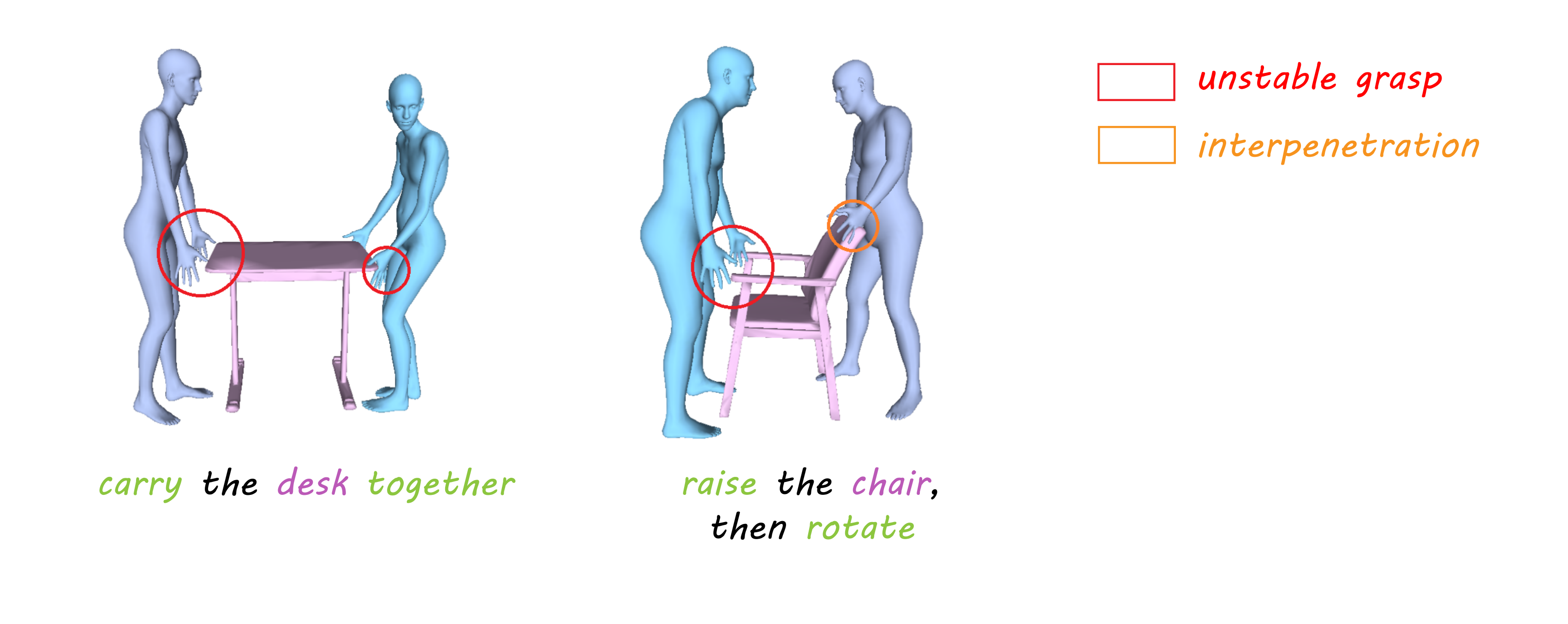
Figure 8: Qualitative results from CORE4D [100] dataset.

5. Irrelevant Body Trajectory Interference. For irrelevant bodies that have already completed the interaction or have not yet joined the interactions, SyncDiff sometimes fails to effectively plan a joining or leaving way for them, leading to interference with subsequent interactions. We provide three samples from CORE4D in the Failure Cases section in the supplementary visualization results for illustration.

6. Rotation Instability. $SO(3)$ is not isomorphic to Euclidean space, and quaternions sometimes fail to maintain stability, especially after introducing decomposition based on frequencies. This usually occurs in cases where objects need to undergo large rotations, such as some types of tools in TACO. We provide three samples from TACO in the Failure Cases section in the supplementary visualization results for illustration.

7. Limitations in Pure Multi-human Interaction Synthesis. Since our relative representations need to be generated in the rigid body coordinate system, our method may not be adapted for pure multi-human interaction synthesis. However, by designing more complex relative representations, this limitation could potentially be addressed.

References

- Arrigoni et al. [2016] Federica Arrigoni, Beatrice Rossi, and Andrea Fusiello. Spectral synchronization of multiple views in se(3). SIAM Journal on Imaging Sciences, 9(4):1963–1990, 2016.
- Brahmbhatt et al. [2019] Samarth Brahmbhatt, Cusuh Ham, Charles C. Kemp, and James Hays. Contactdb: Analyzing and predicting grasp contact via thermal imaging, 2019.
- Brahmbhatt et al. [2020] Samarth Brahmbhatt, Chengcheng Tang, Christopher D Twigg, Charles C Kemp, and James Hays. Contactpose: A dataset of grasps with object contact and hand pose. In Computer Vision–ECCV 2020: 16th European Conference, Glasgow, UK, August 23–28, 2020, Proceedings, Part XIII 16, pages 361–378. Springer, 2020.
- Cha et al. [2024] Junuk Cha, Jihyeon Kim, Jae Shin Yoon, and Seungryul Baek. Text2hoi: Text-guided 3d motion generation for hand-object interaction. In Proceedings of the IEEE/CVF Conference on Computer Vision and Pattern Recognition, pages 1577–1585, 2024.
- Chao et al. [2021] Yu-Wei Chao, Wei Yang, Yu Xiang, Pavlo Molchanov, Ankur Handa, Jonathan Tremblay, Yashraj S. Narang, Karl Van Wyk, Umar Iqbal, Stan Birchfield, Jan Kautz, and Dieter Fox. Dexycb: A benchmark for capturing hand grasping of objects, 2021.
- Chaturvedi et al. [2011] Nalin Chaturvedi, Amit Sanyal, and N. H. Mcclamroch. Rigid-body attitude control. IEEE Control Systems, 31:30–51, 2011.
- Chen et al. [2023] Sirui Chen, Albert Wu, and C. Karen Liu. Synthesizing dexterous nonprehensile pregrasp for ungraspable objects. In Special Interest Group on Computer Graphics and Interactive Techniques Conference Conference Proceedings, page 1–10. ACM, 2023.
- Chen et al. [2019] Ti Chen, Jinjun Shan, and Hao Wen. Distributed adaptive attitude control for networked underactuated flexible spacecraft. IEEE Transactions on Aerospace and Electronic Systems, 55(1):215–225, 2019.
- Choi et al. [2021] Jooyoung Choi, Sungwon Kim, Yonghyun Jeong, Youngjune Gwon, and Sungroh Yoon. Ilvr: Conditioning method for denoising diffusion probabilistic models. arXiv preprint arXiv:2108.02938, 2021.
- Christen et al. [2022a] Sammy Christen, Muhammed Kocabas, Emre Aksan, Jemin Hwangbo, Jie Song, and Otmar Hilliges. D-grasp: Physically plausible dynamic grasp synthesis for hand-object interactions. In Proceedings of the IEEE/CVF Conference on Computer Vision and Pattern Recognition, pages 20577–20586, 2022a.
- Christen et al. [2022b] Sammy Christen, Muhammed Kocabas, Emre Aksan, Jemin Hwangbo, Jie Song, and Otmar Hilliges. D-grasp: Physically plausible dynamic grasp synthesis for hand-object interactions. In Proceedings of the IEEE/CVF Conference on Computer Vision and Pattern Recognition, pages 20577–20586, 2022b.
- Christen et al. [2023] Sammy Christen, Wei Yang, Claudia Pérez-D’Arpino, Otmar Hilliges, Dieter Fox, and Yu-Wei Chao. Learning human-to-robot handovers from point clouds. In Proceedings of the IEEE/CVF Conference on Computer Vision and Pattern Recognition, pages 9654–9664, 2023.
- Christen et al. [2024] Sammy Christen, Shreyas Hampali, Fadime Sener, Edoardo Remelli, Tomas Hodan, Eric Sauser, Shugao Ma, and Bugra Tekin. Diffh2o: Diffusion-based synthesis of hand-object interactions from textual descriptions, 2024.
- Daiya et al. [2024] Divyanshu Daiya, Damon Conover, and Aniket Bera. Collage: Collaborative human-agent interaction generation using hierarchical latent diffusion and language models, 2024.
- Davis et al. [2015] Abe Davis, Justin G. Chen, and Frédo Durand. Image-space modal bases for plausible manipulation of objects in video. ACM Transactions on Graphics (SIGGRAPH), 34(6):1–7, 2015.
- Davis [2016] Myers Abraham Davis. Visual vibration analysis. PhD thesis, Massachusetts Institute of Technology, 2016.
- Dhariwal and Nichol [2021] Prafulla Dhariwal and Alexander Nichol. Diffusion models beat gans on image synthesis. Advances in neural information processing systems, 34:8780–8794, 2021.
- Diener et al. [2009] Julien Diener, Mathieu Rodriguez, Lionel Baboud, and Lionel Reveret. Wind projection basis for real-time animation of trees. In Computer Graphics Forum, pages 533–540. Wiley Online Library, 2009.
- Diller and Dai [2024] Christian Diller and Angela Dai. Cg-hoi: Contact-guided 3d human-object interaction generation. In Proceedings of the IEEE/CVF Conference on Computer Vision and Pattern Recognition, pages 19888–19901, 2024.
- Fan et al. [2023] Zicong Fan, Omid Taheri, Dimitrios Tzionas, Muhammed Kocabas, Manuel Kaufmann, Michael J. Black, and Otmar Hilliges. Arctic: A dataset for dexterous bimanual hand-object manipulation, 2023.
- Garcia-Hernando et al. [2020] Guillermo Garcia-Hernando, Edward Johns, and Tae-Kyun Kim. Physics-based dexterous manipulations with estimated hand poses and residual reinforcement learning, 2020.
- Ghosh et al. [2023] Anindita Ghosh, Rishabh Dabral, Vladislav Golyanik, Christian Theobalt, and Philipp Slusallek. Imos: Intent-driven full-body motion synthesis for human-object interactions. In Computer Graphics Forum, pages 1–12. Wiley Online Library, 2023.
- Haarnoja et al. [2018] Tuomas Haarnoja, Aurick Zhou, Kristian Hartikainen, George Tucker, Sehoon Ha, Jie Tan, Vikash Kumar, Henry Zhu, Abhishek Gupta, Pieter Abbeel, et al. Soft actor-critic algorithms and applications. arXiv preprint arXiv:1812.05905, 2018.
- Hampali et al. [2020] Shreyas Hampali, Mahdi Rad, Markus Oberweger, and Vincent Lepetit. Honnotate: A method for 3d annotation of hand and object poses, 2020.
- Hassan et al. [2021] Mohamed Hassan, Duygu Ceylan, Ruben Villegas, Jun Saito, Jimei Yang, Yi Zhou, and Michael Black. Stochastic scene-aware motion prediction, 2021.
- Hatanaka et al. [2012] Takeshi Hatanaka, Yuji Igarashi, Masayuki Fujita, and Mark W. Spong. Passivity-based pose synchronization in three dimensions. IEEE Transactions on Automatic Control, 57(2):360–375, 2012.
- Ho and Salimans [2022] Jonathan Ho and Tim Salimans. Classifier-free diffusion guidance. arXiv preprint arXiv:2207.12598, 2022.
- Ho et al. [2020] Jonathan Ho, Ajay Jain, and Pieter Abbeel. Denoising diffusion probabilistic models, 2020.
- Ho et al. [2022a] Jonathan Ho, William Chan, Chitwan Saharia, Jay Whang, Ruiqi Gao, Alexey Gritsenko, Diederik P Kingma, Ben Poole, Mohammad Norouzi, David J Fleet, et al. Imagen video: High definition video generation with diffusion models. arXiv preprint arXiv:2210.02303, 2022a.
- Ho et al. [2022b] Jonathan Ho, Tim Salimans, Alexey Gritsenko, William Chan, Mohammad Norouzi, and David J Fleet. Video diffusion models. Advances in Neural Information Processing Systems, 35:8633–8646, 2022b.
- Igarashi et al. [2009] Yuji Igarashi, Takeshi Hatanaka, Masayuki Fujita, and Mark W. Spong. Passivity-based attitude synchronization in . IEEE Transactions on Control Systems Technology, 17(5):1119–1134, 2009.
- Janner et al. [2022] Michael Janner, Yilun Du, Joshua B Tenenbaum, and Sergey Levine. Planning with diffusion for flexible behavior synthesis. arXiv preprint arXiv:2205.09991, 2022.
- Jian et al. [2023] Juntao Jian, Xiuping Liu, Manyi Li, Ruizhen Hu, and Jian Liu. Affordpose: A large-scale dataset of hand-object interactions with affordance-driven hand pose. In Proceedings of the IEEE/CVF International Conference on Computer Vision, pages 14713–14724, 2023.
- Jin et al. [2020] Xin Jin, Yang Shi, Yang Tang, and Xiaotai Wu. Event-triggered attitude consensus with absolute and relative attitude measurements. Automatica, 122:109245, 2020.
- Kingma [2013] Diederik P Kingma. Auto-encoding variational bayes. arXiv preprint arXiv:1312.6114, 2013.
- Krebs et al. [2021] Franziska Krebs, Andre Meixner, Isabel Patzer, and Tamim Asfour. The kit bimanual manipulation dataset. In 2020 IEEE-RAS 20th International Conference on Humanoid Robots (Humanoids), pages 499–506. IEEE, 2021.
- Kwon et al. [2021] Taein Kwon, Bugra Tekin, Jan Stuhmer, Federica Bogo, and Marc Pollefeys. H2o: Two hands manipulating objects for first person interaction recognition, 2021.
- Li et al. [2022] Haoming Li, Xinzhuo Lin, Yang Zhou, Xiang Li, Yuchi Huo, Jiming Chen, and Qi Ye. Contact2grasp: 3d grasp synthesis via hand-object contact constraint. arXiv preprint arXiv:2210.09245, 2022.
- Li et al. [2023a] Jiaman Li, Alexander Clegg, Roozbeh Mottaghi, Jiajun Wu, Xavier Puig, and C Karen Liu. Controllable human-object interaction synthesis. arXiv preprint arXiv:2312.03913, 2023a.
- Li et al. [2023b] Jiaman Li, Jiajun Wu, and C. Karen Liu. Object motion guided human motion synthesis, 2023b.
- Li et al. [2024] Zhengqi Li, Richard Tucker, Noah Snavely, and Aleksander Holynski. Generative image dynamics, 2024.
- Liang et al. [2024] Han Liang, Wenqian Zhang, Wenxuan Li, Jingyi Yu, and Lan Xu. Intergen: Diffusion-based multi-human motion generation under complex interactions. International Journal of Computer Vision, 132(9):3463–3483, 2024.
- Liu et al. [2023a] Qingtao Liu, Yu Cui, Zhengnan Sun, Haoming Li, Gaofeng Li, Lin Shao, Jiming Chen, and Qi Ye. Dexrepnet: Learning dexterous robotic grasping network with geometric and spatial hand-object representations. arXiv preprint arXiv:2303.09806, 2023a.
- Liu et al. [2023b] Shaowei Liu, Yang Zhou, Jimei Yang, Saurabh Gupta, and Shenlong Wang. Contactgen: Generative contact modeling for grasp generation. In Proceedings of the IEEE/CVF International Conference on Computer Vision, pages 20609–20620, 2023b.
- Liu et al. [2022] Yunze Liu, Yun Liu, Che Jiang, Kangbo Lyu, Weikang Wan, Hao Shen, Boqiang Liang, Zhoujie Fu, He Wang, and Li Yi. Hoi4d: A 4d egocentric dataset for category-level human-object interaction. In Proceedings of the IEEE/CVF Conference on Computer Vision and Pattern Recognition, pages 21013–21022, 2022.
- Liu et al. [2024] Yun Liu, Haolin Yang, Xu Si, Ling Liu, Zipeng Li, Yuxiang Zhang, Yebin Liu, and Li Yi. Taco: Benchmarking generalizable bimanual tool-action-object understanding, 2024.
- Liu and Chopra [2012] Yen-Chen Liu and Nikhil Chopra. Controlled synchronization of heterogeneous robotic manipulators in the task space. IEEE Transactions on Robotics, 28(1):268–275, 2012.
- Lugmayr et al. [2022] Andreas Lugmayr, Martin Danelljan, Andres Romero, Fisher Yu, Radu Timofte, and Luc Van Gool. Repaint: Inpainting using denoising diffusion probabilistic models. In Proceedings of the IEEE/CVF conference on computer vision and pattern recognition, pages 11461–11471, 2022.
- Makoviychuk et al. [2021] Viktor Makoviychuk, Lukasz Wawrzyniak, Yunrong Guo, Michelle Lu, Kier Storey, Miles Macklin, David Hoeller, Nikita Rudin, Arthur Allshire, Ankur Handa, et al. Isaac gym: High performance gpu-based physics simulation for robot learning. arXiv preprint arXiv:2108.10470, 2021.
- Mandikal and Grauman [2021] Priyanka Mandikal and Kristen Grauman. Learning dexterous grasping with object-centric visual affordances, 2021.
- Markdahl [2022] Johan Markdahl. Synchronization on riemannian manifolds: Multiply connected implies multistable, 2022.
- Markdahl et al. [2022] Johan Markdahl, Johan Thunberg, and Jorge Goncalves. High-dimensional kuramoto models on stiefel manifolds synchronize complex networks almost globally, 2022.
- Meng et al. [2010] Ziyang Meng, Wei Ren, and Zheng You. Distributed finite-time attitude containment control for multiple rigid bodies. Automatica, 46(12):2092–2099, 2010.
- Mir et al. [2023] Aymen Mir, Xavier Puig, Angjoo Kanazawa, and Gerard Pons-Moll. Generating continual human motion in diverse 3d scenes, 2023.
- Pavlakos et al. [2019] Georgios Pavlakos, Vasileios Choutas, Nima Ghorbani, Timo Bolkart, Ahmed A. A. Osman, Dimitrios Tzionas, and Michael J. Black. Expressive body capture: 3d hands, face, and body from a single image, 2019.
- Peng et al. [2024] Xiaogang Peng, Yiming Xie, Zizhao Wu, Varun Jampani, Deqing Sun, and Huaizu Jiang. Hoi-diff: Text-driven synthesis of 3d human-object interactions using diffusion models, 2024.
- Prokudin et al. [2019] Sergey Prokudin, Christoph Lassner, and Javier Romero. Efficient learning on point clouds with basis point sets, 2019.
- Qi et al. [2017a] Charles R. Qi, Hao Su, Kaichun Mo, and Leonidas J. Guibas. Pointnet: Deep learning on point sets for 3d classification and segmentation, 2017a.
- Qi et al. [2017b] Charles R. Qi, Li Yi, Hao Su, and Leonidas J. Guibas. Pointnet++: Deep hierarchical feature learning on point sets in a metric space, 2017b.
- Qin et al. [2022] Yuzhe Qin, Yueh-Hua Wu, Shaowei Liu, Hanwen Jiang, Ruihan Yang, Yang Fu, and Xiaolong Wang. Dexmv: Imitation learning for dexterous manipulation from human videos, 2022.
- Radford et al. [2021] Alec Radford, Jong Wook Kim, Chris Hallacy, Aditya Ramesh, Gabriel Goh, Sandhini Agarwal, Girish Sastry, Amanda Askell, Pamela Mishkin, Jack Clark, Gretchen Krueger, and Ilya Sutskever. Learning transferable visual models from natural language supervision, 2021.
- Rajeswaran et al. [2018] Aravind Rajeswaran, Vikash Kumar, Abhishek Gupta, Giulia Vezzani, John Schulman, Emanuel Todorov, and Sergey Levine. Learning complex dexterous manipulation with deep reinforcement learning and demonstrations, 2018.
- Ren [2009] Wei Ren. Distributed leaderless consensus algorithms for networked euler–lagrange systems. International Journal of Control, 82:2137–2149, 2009.
- Rombach et al. [2022] Robin Rombach, Andreas Blattmann, Dominik Lorenz, Patrick Esser, and Björn Ommer. High-resolution image synthesis with latent diffusion models. In Proceedings of the IEEE/CVF conference on computer vision and pattern recognition, pages 10684–10695, 2022.
- Romero et al. [2017] Javier Romero, Dimitrios Tzionas, and Michael J. Black. Embodied hands: modeling and capturing hands and bodies together. ACM Transactions on Graphics, 36(6):1–17, 2017.
- Sarlette et al. [2007] Alain Sarlette, Rodolphe Sepulchre, and Naomi Ehrich Leonard. Autonomous rigid body attitude synchronization. In 2007 46th IEEE Conference on Decision and Control, pages 2566–2571, 2007.
- Schulman et al. [2017] John Schulman, Filip Wolski, Prafulla Dhariwal, Alec Radford, and Oleg Klimov. Proximal policy optimization algorithms. arXiv preprint arXiv:1707.06347, 2017.
- Shafir et al. [2023] Yonatan Shafir, Guy Tevet, Roy Kapon, and Amit H. Bermano. Human motion diffusion as a generative prior, 2023.
- Shimada et al. [2023] Soshi Shimada, Franziska Mueller, Jan Bednarik, Bardia Doosti, Bernd Bickel, Danhang Tang, Vladislav Golyanik, Jonathan Taylor, Christian Theobalt, and Thabo Beeler. Macs: Mass conditioned 3d hand and object motion synthesis, 2023.
- Shinya and Fournier [1992] Mikio Shinya and Alain Fournier. Stochastic motion—motion under the influence of wind. Computer Graphics Forum, 11(3), 1992.
- Sohl-Dickstein et al. [2015] Jascha Sohl-Dickstein, Eric A. Weiss, Niru Maheswaranathan, and Surya Ganguli. Deep unsupervised learning using nonequilibrium thermodynamics, 2015.
- Sohn et al. [2015] Kihyuk Sohn, Honglak Lee, and Xinchen Yan. Learning structured output representation using deep conditional generative models. Advances in neural information processing systems, 28, 2015.
- Song et al. [2020] Jiaming Song, Chenlin Meng, and Stefano Ermon. Denoising diffusion implicit models. arXiv preprint arXiv:2010.02502, 2020.
- Song and Ermon [2020] Yang Song and Stefano Ermon. Generative modeling by estimating gradients of the data distribution, 2020.
- Stam [1995] Jos Stam. Multi-scale stochastic modelling of complex natural phenomena. PhD thesis, 1995.
- Stam [1997] Jos Stam. Stochastic dynamics: Simulating the effects of turbulence on flexible structures. Computer Graphics Forum, 16(3), 1997.
- Taheri et al. [2020] Omid Taheri, Nima Ghorbani, Michael J Black, and Dimitrios Tzionas. Grab: A dataset of whole-body human grasping of objects. In Computer Vision–ECCV 2020: 16th European Conference, Glasgow, UK, August 23–28, 2020, Proceedings, Part IV 16, pages 581–600. Springer, 2020.
- Taheri et al. [2022] Omid Taheri, Vasileios Choutas, Michael J Black, and Dimitrios Tzionas. Goal: Generating 4d whole-body motion for hand-object grasping. In Proceedings of the IEEE/CVF Conference on Computer Vision and Pattern Recognition, pages 13263–13273, 2022.
- Tevet et al. [2022] Guy Tevet, Sigal Raab, Brian Gordon, Yonatan Shafir, Daniel Cohen-Or, and Amit H Bermano. Human motion diffusion model. arXiv preprint arXiv:2209.14916, 2022.
- Thunberg et al. [2015] Johan Thunberg, Xiaoming Hu, and Jorge Goncalves. Consensus and formation control on se(3) for switching topologies, 2015.
- Thunberg et al. [2018a] Johan Thunberg, Johan Markdahl, Florian Bernard, and Jorge Goncalves. A lifting method for analyzing distributed synchronization on the unit sphere, 2018a.
- Thunberg et al. [2018b] Johan Thunberg, Johan Markdahl, and Jorge Goncalves. Dynamic controllers for column synchronization of rotation matrices: a qr-factorization approach, 2018b.
- Todorov et al. [2012] Emanuel Todorov, Tom Erez, and Yuval Tassa. Mujoco: A physics engine for model-based control. In 2012 IEEE/RSJ international conference on intelligent robots and systems, pages 5026–5033. IEEE, 2012.
- Wan et al. [2023] Weikang Wan, Haoran Geng, Yun Liu, Zikang Shan, Yaodong Yang, Li Yi, and He Wang. Unidexgrasp++: Improving dexterous grasping policy learning via geometry-aware curriculum and iterative generalist-specialist learning. In Proceedings of the IEEE/CVF International Conference on Computer Vision, pages 3891–3902, 2023.
- Wang [2013] Hanlei Wang. Flocking of networked uncertain euler–lagrange systems on directed graphs. Automatica, 49(9):2774–2779, 2013.
- Wang [2014] Hanlei Wang. Consensus of networked mechanical systems with communication delays: A unified framework. IEEE Transactions on Automatic Control, 59(6):1571–1576, 2014.
- Wang et al. [2021a] Jiashun Wang, Huazhe Xu, Jingwei Xu, Sifei Liu, and Xiaolong Wang. Synthesizing long-term 3d human motion and interaction in 3d scenes, 2021a.
- Wang et al. [2021b] Jingbo Wang, Sijie Yan, Bo Dai, and Dahua LIn. Scene-aware generative network for human motion synthesis, 2021b.
- Wang et al. [2024] Zifan Wang, Junyu Chen, Ziqing Chen, Pengwei Xie, Rui Chen, and Li Yi. Genh2r: Learning generalizable human-to-robot handover via scalable simulation, demonstration, and imitation, 2024.
- Wu et al. [2024a] Qianyang Wu, Ye Shi, Xiaoshui Huang, Jingyi Yu, Lan Xu, and Jingya Wang. Thor: Text to human-object interaction diffusion via relation intervention. arXiv preprint arXiv:2403.11208, 2024a.
- Wu et al. [2024b] Zhen Wu, Jiaman Li, and C Karen Liu. Human-object interaction from human-level instructions. arXiv preprint arXiv:2406.17840, 2024b.
- Xu et al. [2024] Haiyang Xu, Yu Lei, Zeyuan Chen, Xiang Zhang, Yue Zhao, Yilin Wang, and Zhuowen Tu. Bayesian diffusion models for 3d shape reconstruction. In Proceedings of the IEEE/CVF Conference on Computer Vision and Pattern Recognition, pages 10628–10638, 2024.
- Xu et al. [2023] Sirui Xu, Zhengyuan Li, Yu-Xiong Wang, and Liang-Yan Gui. Interdiff: Generating 3d human-object interactions with physics-informed diffusion. In Proceedings of the IEEE/CVF International Conference on Computer Vision, pages 14928–14940, 2023.
- Yang et al. [2021] Lixin Yang, Xinyu Zhan, Kailin Li, Wenqiang Xu, Jiefeng Li, and Cewu Lu. Cpf: Learning a contact potential field to model the hand-object interaction. In Proceedings of the IEEE/CVF International Conference on Computer Vision, pages 11097–11106, 2021.
- Yang et al. [2022] Lixin Yang, Kailin Li, Xinyu Zhan, Fei Wu, Anran Xu, Liu Liu, and Cewu Lu. Oakink: A large-scale knowledge repository for understanding hand-object interaction, 2022.
- Ye et al. [2023] Yufei Ye, Xueting Li, Abhinav Gupta, Shalini De Mello, Stan Birchfield, Jiaming Song, Shubham Tulsiani, and Sifei Liu. Affordance diffusion: Synthesizing hand-object interactions. In Proceedings of the IEEE/CVF Conference on Computer Vision and Pattern Recognition, pages 22479–22489, 2023.
- Yi et al. [2025] Hongwei Yi, Justus Thies, Michael J Black, Xue Bin Peng, and Davis Rempe. Generating human interaction motions in scenes with text control. In European Conference on Computer Vision, pages 246–263. Springer, 2025.
- Yuan et al. [2023] Ye Yuan, Jiaming Song, Umar Iqbal, Arash Vahdat, and Jan Kautz. Physdiff: Physics-guided human motion diffusion model. In Proceedings of the IEEE/CVF international conference on computer vision, pages 16010–16021, 2023.
- Zhan et al. [2024] Xinyu Zhan, Lixin Yang, Yifei Zhao, Kangrui Mao, Hanlin Xu, Zenan Lin, Kailin Li, and Cewu Lu. Oakink2: A dataset of bimanual hands-object manipulation in complex task completion, 2024.
- Zhang et al. [2024a] Chengwen Zhang, Yun Liu, Ruofan Xing, Bingda Tang, and Li Yi. Core4d: A 4d human-object-human interaction dataset for collaborative object rearrangement, 2024a.
- Zhang et al. [2021] He Zhang, Yuting Ye, Takaaki Shiratori, and Taku Komura. Manipnet: neural manipulation synthesis with a hand-object spatial representation. ACM Transactions on Graphics (ToG), 40(4):1–14, 2021.
- Zhang et al. [2024b] Hui Zhang, Sammy Christen, Zicong Fan, Luocheng Zheng, Jemin Hwangbo, Jie Song, and Otmar Hilliges. Artigrasp: Physically plausible synthesis of bi-manual dexterous grasping and articulation, 2024b.
- Zhang et al. [2025] Hui Zhang, Sammy Christen, Zicong Fan, Otmar Hilliges, and Jie Song. Graspxl: Generating grasping motions for diverse objects at scale. In European Conference on Computer Vision, pages 386–403. Springer, 2025.
- Zhang et al. [2024c] Jiajun Zhang, Yuxiang Zhang, Liang An, Mengcheng Li, Hongwen Zhang, Zonghai Hu, and Yebin Liu. Manidext: Hand-object manipulation synthesis via continuous correspondence embeddings and residual-guided diffusion. arXiv preprint arXiv:2409.09300, 2024c.
- Zhang et al. [2023] Lvmin Zhang, Anyi Rao, and Maneesh Agrawala. Adding conditional control to text-to-image diffusion models. In Proceedings of the IEEE/CVF International Conference on Computer Vision, pages 3836–3847, 2023.
- Zhang et al. [2022a] Mingyuan Zhang, Zhongang Cai, Liang Pan, Fangzhou Hong, Xinying Guo, Lei Yang, and Ziwei Liu. Motiondiffuse: Text-driven human motion generation with diffusion model. arXiv preprint arXiv:2208.15001, 2022a.
- Zhang et al. [2024d] Wanyue Zhang, Rishabh Dabral, Vladislav Golyanik, Vasileios Choutas, Eduardo Alvarado, Thabo Beeler, Marc Habermann, and Christian Theobalt. Bimart: A unified approach for the synthesis of 3d bimanual interaction with articulated objects. arXiv preprint arXiv:2412.05066, 2024d.
- Zhang et al. [2022b] Xiaohan Zhang, Bharat Lal Bhatnagar, Sebastian Starke, Vladimir Guzov, and Gerard Pons-Moll. Couch: Towards controllable human-chair interactions. In European Conference on Computer Vision, pages 518–535. Springer, 2022b.
- Zhao et al. [2022] Kaifeng Zhao, Shaofei Wang, Yan Zhang, Thabo Beeler, and Siyu Tang. Compositional human-scene interaction synthesis with semantic control. In European Conference on Computer Vision, pages 311–327. Springer, 2022.
- Zhao et al. [2023] Kaifeng Zhao, Yan Zhang, Shaofei Wang, Thabo Beeler, and Siyu Tang. Synthesizing diverse human motions in 3d indoor scenes, 2023.
- Zheng et al. [2023] Juntian Zheng, Qingyuan Zheng, Lixing Fang, Yun Liu, and Li Yi. Cams: Canonicalized manipulation spaces for category-level functional hand-object manipulation synthesis. In Proceedings of the IEEE/CVF Conference on Computer Vision and Pattern Recognition, pages 585–594, 2023.
- Zhong et al. [2025] Lei Zhong, Yiming Xie, Varun Jampani, Deqing Sun, and Huaizu Jiang. Smoodi: Stylized motion diffusion model. In European Conference on Computer Vision, pages 405–421. Springer, 2025.
- Zhou et al. [2024] Bohan Zhou, Haoqi Yuan, Yuhui Fu, and Zongqing Lu. Learning diverse bimanual dexterous manipulation skills from human demonstrations, 2024.
- Zhou et al. [2022] Keyang Zhou, Bharat Lal Bhatnagar, Jan Eric Lenssen, and Gerard Pons-Moll. Toch: Spatio-temporal object-to-hand correspondence for motion refinement. In European Conference on Computer Vision, pages 1–19. Springer, 2022.
- Zou and Meng [2019] Yao Zou and Ziyang Meng. Velocity-free leader–follower cooperative attitude tracking of multiple rigid bodies on so(3). IEEE Transactions on Cybernetics, 49(12):4078–4089, 2019.