Pharmacophore-constrained de novo drug design with diffusion bridge

Abstract

De novo design of bioactive drug molecules with potential to treat desired biological targets is a profound task in the drug discovery process. Existing approaches tend to leverage the pocket structure of the target protein to condition the molecule generation. However, even the pocket area of the target protein may contain redundant information since not all atoms in the pocket is responsible for the interaction with the ligand. In this work, we propose PP2Drug - a phamacophore-constrained de novo design approach to generate drug candidate with desired bioactivity. Our method adapts diffusion bridge to effectively convert pharmacophore designs in the spatial space into molecular structures under the manner of equivariant transformation, which provides sophisticated control over optimal biochemical feature arrangement on the generated molecules. PP2Drug is demonstrated to generate hit candidates that exhibit high binding affinity with potential protein targets.

Keywords Diffusion bridge  $\cdot$ Geometric learning  $\cdot$ Drug design

1 Introduction

Computer-aided drug design (CADD) plays a crucial role in the modern drug discovery procedure. However, conventional CADD approaches such as virtual screening are undertaken to search for the candidates with optimal molecular properties in a vast chemistry library. Although accelerated by the high-throughput technology, this process can still be time-consuming and costly [1] since the relationship between chemical structures and the molecular property of interest is obscure. De novo design, on the other hand, models the chemical space of molecular structures and properties and seeks for the optimal candidates in a directed manner [2] instead of enumerating every possibility, thus facilitating the drug discovery process. Moreover, the flourishing of deep generative models in various domains such as large language models and image synthesis has endowed us an opportunity of applying deep learning to improving de novo drug design algorithms.

Generative models including variational autoencoder (VAE) [3], generative adversarial networks (GAN) [4] and denoising diffusion probabilistic models (DDPM) [5], have been successfully adapted for molecular design. Initially, researchers tend to represent drugs with linear notations such as Simplified Molecular-Input Line-Entry System (SMILES) [6] due to its simplicity. Then long-short term memory (LSTM) networks were readily applied to encoding the SMILES notations, and VAE and GAN algorithms were utilized for generation [7, 8, 9, 10]. Such methods, however, suffered from low chemistry validity of generated molecules since the structural information is neglected in SMILES notations.

To alleviate such limitations, a wide range of molecular graph-based generative algorithms has emerged. For example, graph VAE [11] paved the way for probabilistic graph construction approach, which can be used as the generator of other generative models such as GANs [12]. However, due to computational complexity, such methods were only able to generate a limited number of nodes. A couple of research managed to address this issue by proposing auto-regressive graph construction algorithms. Flow-based methods such as MoFlow [13] and GraphAF [14] model the generation of bonds and atoms in a sequential decision flow and generate them in order. MoLeR [15] and MGSSL [16] introduced motif-based generation that considered functional groups rather than single atoms as nodes and thus expanding the scale of generated molecules. Auto-regressive generation also improved the validity rate of generated molecules since valence check can be performed at every step of generation. However, such methods are unnatural since in a molecule, there is no such sequence in which latter atoms depend on former generated ones. In addition, if one step in the middle of the generation is predicted improperly, the whole subsequent generation is affected.

The advent of diffusion models [17] enables molecular graph generation in one-shot. Although diffusion models initially obtained tremendous success in text and image generation [18], a wealth of research have demonstrated that they can be adapted for graph generation as well since they can be developed to learn the distributions of the adjacency matrix and the feature matrix, which fully define the graph [19, 20, 21]. In the meantime, researchers realized the power of diffusion models is not restricted on 2D graph generation and can be evolved into 3D point cloud generation, which allows for more sophisticated design of molecules. In 2D graph generation, subsequent tests over all 3D conformers have to be conducted to filter the candidate since different isomers of a molecule may exhibit various pharmaceutical properties, which may lead to additional costs and future attrition. Aiming at achieving direct 3D spatial design of molecules, a series of studies were proposed [22, 23, 24, 25, 26]. They leveraged equivariant geometric learning to ensure the roto-translational equivariance of their systems while generating coordinates of the nodes.

Nevertheless, latest research indicate that the typical diffusion models such as score matching with Langevin dynamics (SMLD) [27] and DDPM [5] can be generalized as diffusion bridges that are guaranteed to reach an end point from the desirable domain in pre-fixed time [28, 29] according to Doob’s h-transform [30]. Moreover, it is demonstrated that diffusion bridges not only can be applied to unconditional generation by mapping data distribution to the prior noise distribution but also can be leveraged to align any two arbitrary distributions by fixing both the start point and the end point [31, 32, 33]. Diffusion bridges have been successfully adapted for image translation [34, 35], physics-informed molecule generation [36, 37] and molecular docking [38]. We believe they are promising models for hit molecule design as well since the start point can be naturally considered as the molecular structures and the end point as desired conditions, e.g., pharmacophore arrangements.

In the field of drug design, increasing research have delved into adapting generative models to the design of hit candidates with potential to react with particular biological targets. For example, gene expression profiles were used to condition the generation so that the generated molecules may lead to desirable biological activities [8, 9, 10, 39]. However, gene expression profiles may contain redundant information, since not all genes are related with the drug reaction. To enable more sophisticated control over the generation procedure, researchers proceeded to consider the target protein structure as the constraint. Pocket2Mol [40] first proposed an auto-regressive model to generate atoms and bonds gradually under the guidance of the the protein pocket structure. Further research improved pocket-based generation by one-shot generation using diffusion models, such as TargetDiff [26]. D3FG [21] extended atom-based generation to functional group, aiming at preserving better chemical consistency.

Recently, a couple of studies proposed to generate hit candidates constrained by pharmacophores, which hypothesizes a spatial arrangement of chemical features that are essential for the binding between a drug and a target protein. Unlike conditioning by the protein pocket structure, which depends on the model to learn to discover the indispensable features for binding implicitly, pharmacophore arrangements explicitly define such features, which renders them suitable constraints for hit discovery. Nonetheless, existing research studying pharmacophore-based drug discovery, e.g., PharmacoNet [41], only leveraged pharmacophore modelling to compute matching scores between ligand and protein, and thereby accelerated virtual screening. Although PGMG [42] introduced a de novo pharmacophore-guided drug design framework, it only learned a latent variable of the pharmacophore features and generated SMILES representations accordingly. This actually destructs the 3D features given by the pharmacophore hypotheses and omits their connection with the 3D molecular structures. In this work, we propose a direct pharmacophore-constrained de novo drug design approach that learns to transform pharmacophore distributions into molecular structure distributions with equivariant diffusion bridge.

2 Background

Diffusion models including SMLD [27] and DDPM [5] generally construct a probabilistic process to transform a data distribution into a prior distribution by adding noise gradually, which can be reversed so that new data points can be generated from noise sampled from the prior distribution. Song et al. [17] proposed to generalize diffusion models with a framework built on stochastic differential equations (SDEs).

2.1 Diffusion model with SDEs

The diffusion process is to inject noise into data $\mathbf{G}_{0}\sim p_{data}$ and gradually convert data into noise $\mathbf{G}_{T}\sim p_{prior}$, where $p_{data}$ and the $p_{prior}$ denote the data and prior distribution, respectively. Song et al. proposed to model this diffusion process as the following SDE

$$d\mathbf{G}_{t}=\mathbf{f}(\mathbf{G}_{t},t)dt+g(t)d\mathbf{w}_{t}$$ (1)

where $\mathbf{f}$ is the drift function, $\mathbf{w_{t}}$ is the standard Wiener process and $g$ is the diffusion coefficient. In our case, we denote the molecular graph at time $t$ as $\mathbf{G}_{t}$.

The reverse process is also formulated as an SDE

$$d\mathbf{G}_{t}=[\mathbf{f}(\mathbf{G}_{t},t)-g(t)^{2}\nabla_{\mathbf{G}_{t}}\log p(\mathbf{G}_{t})]dt+g(t)d\mathbf{w}_{t}$$ (2)

where $p(\mathbf{G}_{t})$ is the marginal distribution of $\mathbf{G}_{t}$ at time $t$. SMLD and DDPM can be regarded as such SDE framework with different schedules of $\mathbf{f}$ and $g$.

2.2 Diffusion bridge

The diffusion process (1) and the denoising process (2) in the typical diffusion model can be viewed as two diffusion bridge processes, whose end points are fixed at the noise from the prior distribution $\mathbf{G}_{T}\sim p_{prior}$ and the initial data point $\mathbf{G}_{0}\sim p_{data}$, respectively. Moreover, Doob’s $h$-transform [30] reveals that by adding an additional drift term, the original diffusion process (1) is guaranteed to reach a fixed end point from an arbitrary distribution, given by

$$d\mathbf{G}_{t}=[\mathbf{f}(\mathbf{G}_{t},t)+g(t)^{2}\nabla_{\mathbf{G}_{t}}\log p_{T|t}(\mathbf{G}_{T}|\mathbf{G}_{t})]dt+g(t)d\mathbf{w}_{t}$$ (3)

where $p_{T|t}(\mathbf{G}_{T}|\mathbf{G}_{t})$ is the probability density function of transition from $t$ to $T$, which can be directly computed. The additional drift term $g(t)^{2}\nabla_{\mathbf{G}_{t}}\log p_{T|t}(\mathbf{G}_{T}|\mathbf{G}_{t})$ drives $\mathbf{G}_{t}$ to the desired end point $\mathbf{G}_{T}$. In this work, we investigate how to construct the diffusion bridge between molecule graphs $\mathbf{g}\sim p_{mol}$ and pharmacophore graphs $\mathbf{\Gamma}\sim p_{pp}$. Therefore, we set the start point at $\mathbf{G}_{0}=\mathbf{g}$ and the end point at $\mathbf{G}_{T}=\mathbf{\Gamma}$.

3 Pharmacophore to drug diffusion bridge

We introduce the pharmacophore to drug (PP2Drug) diffusion bridge model to translate 3D arrangement of pharmacophore features to generation into hit molecules. The proposed framework in presented in Figure 1.

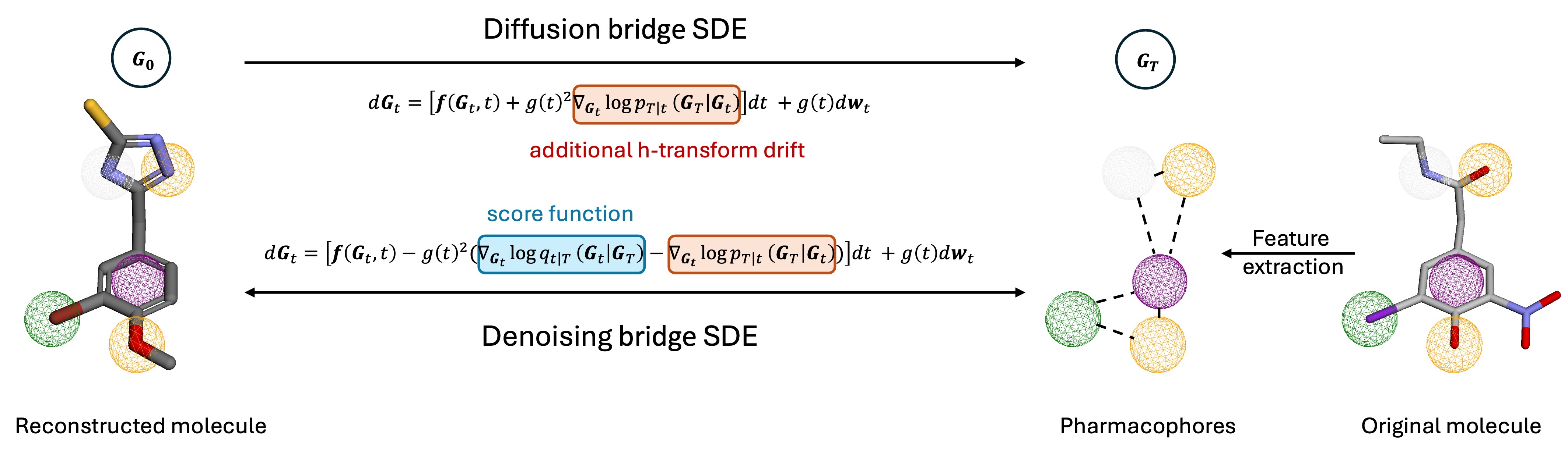
Figure 1: Overview of PP2Drug. The diffusion bridge process is devised to map the molecule data $\mathbf{G}_{0}$ to the extracted pharmacophore data $\mathbf{G}_{T}$ via Doob’s h-transform. Reversely, a score matching model is trained to estimate the score function, which composes the denoising bridge process that recovers molecule data from the pharmacophore data.

3.1 Graph translation via denoising bridge

We introduce a graph translation paradigm that generates 3D point cloud constrained by predefined cluster arrangements. We demonstrate our approach on the task of 3D hit molecule design guided by pharmacophore hypothesis. Based on the diffusion bridge SDE in (3), the corresponding denoising bridge SDE is formulated as

$$d\mathbf{G}_{t}=[\mathbf{f}(\mathbf{G}_{t},t)-g^{2}(t)(\nabla_{\mathbf{G}_{t}}\log q_{t|T}(\mathbf{G}_{t}|\mathbf{G}_{T})-\nabla_{\mathbf{G}_{t}}\log p_{T|t}(\mathbf{G}_{T}|\mathbf{G}_{t}))]dt+g(t)d\mathbf{w}_{t}$$ (4)

where $q_{t|T}(\mathbf{G}_{t}|\mathbf{G}_{T})$ denotes the conditional probability of sampling $\mathbf{G}_{t}$ given $\mathbf{G}_{T}$. The aim is to estimate the score $\nabla_{\mathbf{G}_{t}}\log q_{t|T}(\mathbf{G}_{t}|\mathbf{G}_{T})$ at each time step $t$, thus sampling $\mathbf{G}_{0}$ using the denoising bridge (4).

Denoising score matching

To approximate the denoising bridge process (4), a neural network backbone $s_{\theta}$ is trained to estimate the score of bridge $q$. We follow the typical denoising score matching schema to design the training objective as

$$\mathcal{L}_{\theta}=\mathbb{E}_{\mathbf{G}_{t},\mathbf{G}_{0},\mathbf{G}_{T},t}\left[w(t)\left\|s_{\theta}(\mathbf{G}_{t},\mathbf{G}_{T},t)-\nabla_{\mathbf{G}_{t}}\log q(\mathbf{G}_{t}|\mathbf{G}_{0},\mathbf{G}_{T})\right\|^{2}\right]$$ (5)

where $w(t)$ is a time-dependent loss weighting term to intensifies the penalty as the denoising bridge approaches the data point, enhancing the the accuracy of reconstruction at later stages. Details of the choice of this term will be discussed in next section. It is non-trivial to estimate the true score of $q_{t|T}$ directly. Therefore, we instead train the score model $s_{\theta}$ to approximate the score of a tractable denoising bridge $q(\mathbf{G}_{t}|\mathbf{G}_{0},\mathbf{G}_{T})$ conditioned on both the start point $\mathbf{G}_{0}$ and the end point $\mathbf{G}_{T}$.

3.2 Score model parameterization

To parameterize the score model $s_{\theta}$, we design the denoising bridge $q$ to be a tractable Gaussian distribution that is the same as the diffusion bridge $p$

$$q(\mathbf{G}_{t}|\mathbf{G}_{0},\mathbf{G}_{T}) :=p(\mathbf{G}_{t}|\mathbf{G}_{0},\mathbf{G}_{T})=\mathcal{N}(\hat{\mu}_{t},\hat{\sigma}_{t}^{2}\mathbf{I}),$$ (6)

$$\mathrm{where}\quad\hat{\mu}_{t} =\frac{\text{SNR}_{T}}{\text{SNR}_{t}}\frac{\alpha_{t}}{\alpha_{T}}\mathbf{G}_{T}+\alpha_{t}\mathbf{G}_{0}(1-\frac{\text{SNR}_{T}}{\text{SNR}_{t}})$$

$$\hat{\sigma}_{t}^{2} =\sigma_{t}^{2}(1-\frac{\text{SNR}_{T}}{\text{SNR}_{t}})$$

where $\alpha_{t}$ and $\sigma_{t}$ are the signal and noise schedules, which vary with the choice of the bridge design. Signal-to-noise ratio is thereby defined as $\text{SNR}_{t}=\alpha_{t}^{2}/\sigma_{t}^{2}$

Since the denoising bridge in (6) is designed to be a Gaussian distribution, its score function can be readily derived by

$$\nabla_{\mathbf{G}_{t}}\log q(\mathbf{G}_{t}|\mathbf{G}_{0},\mathbf{G}_{T})=-\frac{\mathbf{G}_{t}-\hat{\mu}_{t}}{\hat{\sigma}_{t}^{2}}$$ (7)

which is estimated by $s_{\theta}(\mathbf{G}_{t},\mathbf{G}_{T},t)$. We further reparameterize $s_{\theta}$ to be

$$s_{\theta}(\mathbf{G}_{t},\mathbf{G}_{T},t)=-\frac{\mathbf{G}_{t}-(\frac{\text{SNR}_{T}}{\text{SNR}_{t}}\frac{\alpha_{t}}{\alpha_{T}}\mathbf{G}_{T}+\alpha_{t}D_{\theta}(\mathbf{G}_{t},\mathbf{G}_{T},t)(1-\frac{\text{SNR}_{T}}{\text{SNR}_{t}}))}{\sigma_{t}^{2}(1-\frac{\text{SNR}_{T}}{\text{SNR}_{t}})}$$ (8)

where $\mathbf{G}_{0}$ is predicted by $D_{\theta}(\mathbf{G}_{t},\mathbf{G}_{T},t)$. Following EDM [43], $D_{\theta}$ can be further reparameterized with

$$D_{\theta}(\mathbf{G}_{t},\mathbf{G}_{T},t)=c_{skip}(t)\mathbf{G}_{t}+c_{out}(t)F_{\theta}(c_{in}(t)\mathbf{G}_{t},c_{noise}(t))$$ (9)

where $F_{\theta}$ is the neural network that predicts something between $\mathbf{G}_{0}$ and the noise at time step $t$. In typical diffusion models [17, 27, 5], $F_{\theta}$ aims at predicting the noise at time step $t$ directly, but this is non-trivial when $t$ is approaching the final step $T$, since the data is almost full of noise. EDM proposed to adapt $F_{\theta}$ to predict the mixture of signal and noise to alleviate this drawback [43].

Scaling designs

Following DDBM [35], our bridge scalings are designed as

$$c_{in}(t)=\frac{1}{\sqrt{a_{t}^{2}\sigma_{T}^{2}+b_{t}^{2}\sigma_{t}^{2}+2a_{t}b_{t}\sigma_{0T}+c_{t}}},$$ (10)

$$c_{out}(t)=\sqrt{a_{t}^{2}(\sigma_{T}^{2}\sigma_{0}^{2}-\sigma_{0T}^{2})+\sigma_{0}^{2}c_{t}}*c_{in}(t),$$

$$c_{skip}(t)=(b_{t}\sigma_{0}^{2}+a_{t}\sigma_{0T})*c_{in}^{2}(t),$$

$$c_{noise}(t)=\frac{1}{4}\log(\sigma_{t}),$$

$$w(t)=\frac{1}{c_{out}(t)^{2}},$$

$$where\quad a_{t}=\frac{\alpha_{t}\text{SNR}_{T}}{\alpha_{T}\text{SNR}_{t}},\quad b_{t}=\alpha_{t}(1-\frac{\text{SNR}_{T}}{\text{SNR}_{t}})\quad and\quad c_{t}=\sigma_{t}^{2}(1-\frac{\text{SNR}_{T}}{\text{SNR}_{t}})$$

where $\sigma_{0}^{2}$ and $\sigma_{T}^{2}$ refer to the variance of the molecular graph $\mathbf{g}$ and the pharmacophore graph $\mathbf{\Gamma}$, respectively. The data variance at $t$-th step is configured as $\sigma_{t}=t$. The choice of $\sigma_{0}$ and $\sigma_{t}$ should be decided via hyper-parameter tuning.

3.2.1 $E(3)$-equivariant network

As illustrated in (8) and (9), the target of our score matching model is finalized to predict the mixture of signal and noise with $F_{\theta}$, which is, in our case, to predict the molecular graphs with certain noise. A molecular graph is defined as $\mathbf{g}=(\mathbf{x}_{mol},\mathbf{h}_{mol})$, where $\mathbf{x}_{mol}\in\mathbb{R}^{N\times 3}$ represents the coordinates of $N$ atoms in the 3D space and $\mathbf{h}_{mol}\in\mathbb{R}^{N\times M}$ represents the node feature matrix that is composed of one-hot encoding of $M$ atom types. A pharmacophore graph is defined as $\mathbf{\Gamma}=(\mathbf{x}_{pp},\mathbf{h}_{pp})$. Similarly, $\mathbf{x}_{pp}\in\mathbb{R}^{N\times 3}$ records the center coordinates of the pharmacophore that each atom belongs to, and $\mathbf{h}_{pp}\in\mathbb{R}^{N\times K}$ is the feature matrix of K pharmacophore types’ one-hot encoding. For data consistency, we perform zero padding to the feature matrix with less number of features, i.e., $\mathbf{h}_{mol},\mathbf{h}_{pp}\in\mathbb{R}^{N\times F}$ with $F=\text{max}(M,K)$. Thus, the behavior of $F_{\theta}$ at time step $t$ is formulated as

$$(\tilde{\mathbf{x}},\tilde{\mathbf{h}})=F_{\theta}(c_{in}(t)\mathbf{G}_{t},c_{noise}(t))=F_{\theta}(c_{in}(t)(\mathbf{x}_{t},\mathbf{h}_{t}),c_{noise}(t))$$ (11)

Equivariance

To manipulate 3D objects, it is crucial that the model $F_{\theta}$ satisfies $E(3)$-equivariance. This ensures, for the coordinates $\mathbf{x}$, transformations such as rotations and translations of the input graph should result in the equivariant output transformations, whereas the node features $\mathbf{h}$ should be invariant to any transformations. Assuming any transformation given by $\mathbf{Rx}+\mathbf{b}$ is undertaken to the input coordinates, an equivariant model should have

$$(\mathbf{R}\tilde{\mathbf{x}}+\mathbf{b},\tilde{\mathbf{h}})=F_{\theta}\left(c_{in}(t)(\mathbf{Rx}+\mathbf{b},\mathbf{h}),c_{noise}(t)\right)$$ (12)

where $\mathbf{R}\in\mathbb{R}^{3}$ is an orthogonal matrix defining the rotation and $\mathbf{b}\in\mathbb{R}^{3}$ defines the translation.

To meet the $E(3)$-equivariant property, we build our model with EGNN [44]. To condition the updating of the molecular graph with the desired pharmacophore models, we concatenate the coordinates and features of the molecular graph at time $t$ and the initial pharmacophore graph to form a combined graph $\mathbf{G}_{t}=(\mathbf{x}_{t},\mathbf{h}_{t})$, where $\mathbf{x}_{t}\in\mathbb{R}^{2N\times 3}$ and $\mathbf{h}_{t}\in\mathbb{R}^{2N\times F}$. A mask $\mathcal{M}^{mol}\in\mathbb{R}^{2N}$ is applied to only update the nodes belonging to the molecular graph.

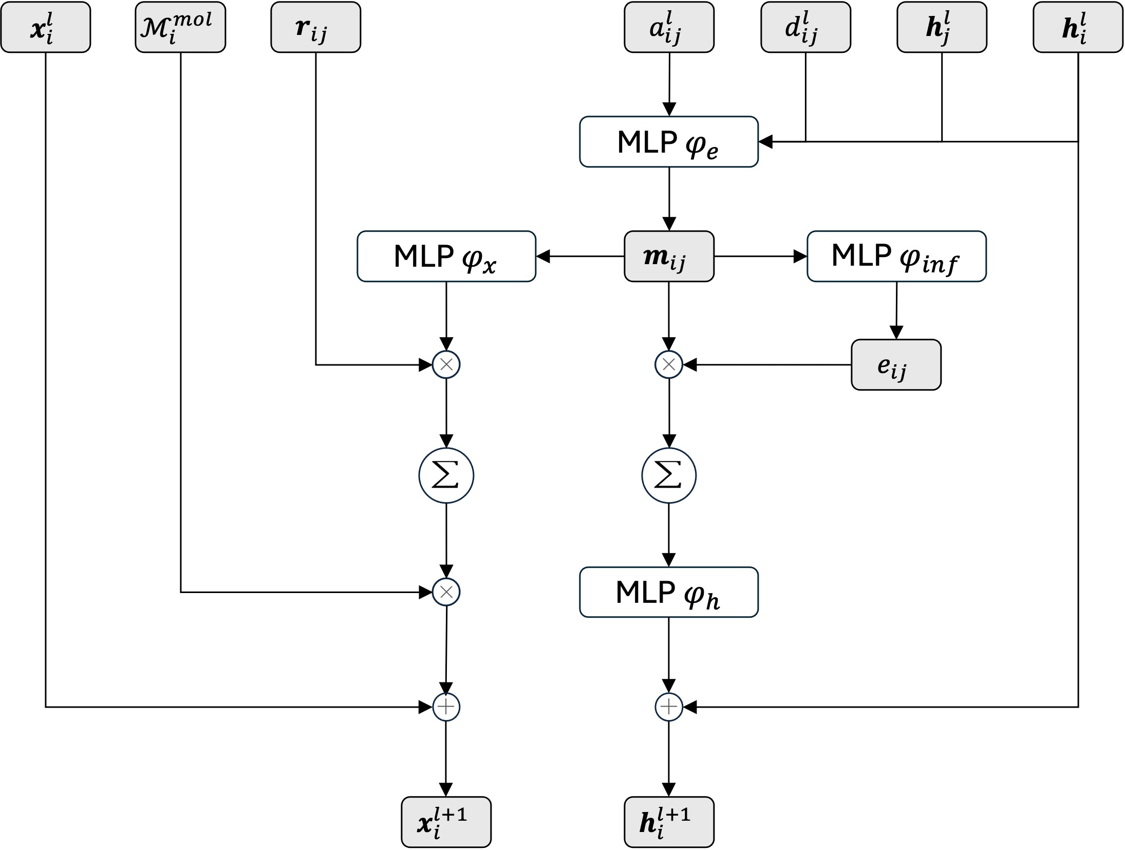
Figure 2: Flowchart of the EGCL module. $\otimes$ and $\oplus$ denote element-wise multiplication and addition, respectively. $\sum$ represents summation over all neighbors.

The Equivariant Graph Convolutional Layer (EGCL) that we used for feature updating is illustrated in Figure 2. At $l$-th layer, the updating procedure is defined as

$$\mathbf{m}_{ij}=\phi_{e}(\mathbf{h}_{i}^{l},\mathbf{h}_{j}^{l},d_{ij}^{2},a_{ij}),$$ (13)

$$\mathbf{h}_{i}^{l+1}=\mathbf{h}_{i}^{l}+\phi_{h}(\mathbf{h}_{i}^{l},\sum_{j\in\mathcal{N}(i)}e_{ij}\mathbf{m}_{ij}),$$

$$\mathbf{x}_{i}^{l+1}=\mathbf{x}_{i}^{l}+\sum_{j\in\mathcal{N}(i)}\mathbf{r}_{ij}\phi_{x}(\mathbf{m}_{ij})\cdot\mathcal{M}^{mol}_{i}$$

where $i$ and $j$ refer to the node index. $d_{ij}=\|\mathbf{x}_{i}-\mathbf{x}_{j}\|$ is the euclidean distance between node $i$ and $j$, and $\mathbf{r}_{ij}=\mathbf{x}_{i}^{l}-\mathbf{x}_{j}^{l}$ is the vector difference between node $i$ and $j$. $a_{ij}$ is the edge attribute indicating the interaction is between atoms, pharmacophore nodes, or an atom and a pharmacophore node. $e_{ij}$ is the soft estimation of the existence of edge between node $i$ and $j$, which is computed by $e_{ij}=\phi_{inf}(\mathbf{m}_{ij})$. Initially, the time step $t_{i}$ is incorporated with $\mathbf{h}_{i}^{0}$ via $\mathbf{h}_{i}^{0}=\phi_{time}(\mathbf{h}_{i}^{0},t_{i})$. $\phi_{time}$, $\phi_{e}$, $\phi_{h}$, $\phi_{x}$ and $\phi_{inf}$ are all trainable MLPs. As demonstrated by TargetDiff [26], EGCL governs the rotational equivariance. To fulfill translational equivariance as well, we must shift the center of the pharmacophore graph to zero.

3.2.2 Training objective

Based on the output of $F_{\theta}$ in (11), we can readily obtain the denoised position matrix $\hat{\mathbf{x}}_{0}=c_{skip}(t)\mathbf{x}_{t}+c_{out}(t)\tilde{\mathbf{x}}$ and the denoised feature matrix $\hat{\mathbf{h}}_{0}=c_{skip}(t)\mathbf{h}_{t}+c_{out}(t)\tilde{\mathbf{h}}$ of the original molecular graph predicted by the denoiser $D_{\theta}$. Practically, the loss function in (5) is equivalent to

$$\mathcal{L}_{\theta}=\mathbb{E}_{\mathbf{x}_{t},\mathbf{x}_{0},\mathbf{h}_{t},\mathbf{h}_{0},t}(\|\hat{\mathbf{x}}_{0}-\mathbf{x}_{0}\|^{2}+\lambda\|\hat{\mathbf{h}}_{0}-\mathbf{h}_{0}\|^{2})$$ (14)

which is the combination of the MSE losses with regard to $\mathbf{x}$ and $\mathbf{h}$. The weight of feature loss $\lambda$ is empirically configured as 10 to keep the training stable.

3.3 Sampling with PP2Drug

Algorithm 1 Stochastic sampler of PP2Drug

Input: sampled time steps $t_{i\in{N,...,0}}$, pharmacophore data $\mathbf{G}_{N}\sim p_{pp}$, score matching model $\mathbf{s}_{\theta}$

for $i=N:1$ do

     $\mathbf{d}_{i}\leftarrow-\mathbf{f}(\mathbf{G}_{i},t_{i})+g^{2}(t_{i})(\mathbf{s}_{\theta}(\mathbf{G}_{i},\mathbf{G}_{N},T)-\nabla_{\mathbf{G}_{i}}\log p(\mathbf{G}_{N}|\mathbf{G}_{i})))$ $\triangleright$ Solving Eq. 4

     $\mathbf{G}_{i-1}\leftarrow\mathbf{G}_{i}+(t_{i-1}-t_{i})\mathbf{d}_{i}$ $\triangleright$ Euler step

     if $i\neq 1$ then

         $\mathbf{d}_{i}^{\prime}\leftarrow-\mathbf{f}(\mathbf{G}_{i-1},t_{i-1})+g^{2}(t_{i-1})(\frac{1}{2}\mathbf{s}_{\theta}(\mathbf{G}_{i-1},\mathbf{G}_{N},T)-\nabla_{\mathbf{G}_{i-1}}\log p(\mathbf{G}_{N}|\mathbf{G}_{i-1})))$

         $\mathbf{G}_{i-1}\leftarrow\mathbf{G}_{i}+(t_{i+1}-t_{i})(\frac{1}{2}\mathbf{d}_{i}+\frac{1}{2}\mathbf{d}_{i}^{\prime})$ $\triangleright$ Heun’s 2nd order correction

     end if

end for

return $\mathbf{G}_{0}$

Our stochastic sampler is adapted from the Heun’s 2nd order sampler in EDM [43]. We first discretize the time steps according to

$$t_{i}=(\sigma_{max}^{\frac{1}{\rho}}+\frac{N-i}{N-1}(\sigma_{min}^{\frac{1}{\rho}}-\sigma_{max}^{\frac{1}{\rho}}))^{\rho},\quad when\quad i>0$$ (15)

where $\rho$ is a parameter to control that shorter steps are take near $\sigma_{min}$, and is set to $\rho=7$ by default. We set $t_{0}=0$ to ensure the output is the reconstructed data sample. Empirically, for VE bridge, we set $\sigma_{min}=0.02$ and $\sigma_{max}=80$. And for VP bridge, we set $\sigma_{min}=0.0001$ and $\sigma_{max}=1$.

Alg. 1 illustrates the sampling procedure of our model. The output of the score matching model $\mathbf{s}_{\theta}$ is computed via Eq. 8 and 9. The h-transform drift $\nabla_{\mathbf{G}_{i}}\log p(\mathbf{G}_{N}|\mathbf{G}_{i})$ is derived by calculating the score of the transition probability from $t_{i}$ to $t_{N}$. This computation is tractable when using VE and VP bridge designs, since both devise the probability density function $p_{T|t}$ as Gaussian transition kernel.

4 Experiments

4.1 Experimental Setup

Data

Crossdocked2020 V1.3 dataset [45] is used for model development and evaluation. Following TargetDiff [26], we filter the dataset by preserving only the ligands with intimate protein binding poses (RMSE $<$ 0.1 Å), which results in around 242 thousand ligands. Crossdocked2020 data has organized the ligand and protein files according to pockets. We therefore split the dataset in the same way, ensuring molecules with similar structures or biological targets occur either in training or sampling dataset. 80% of the pockets are used for training, 10% for validation and 10% for testing, resulting in around 197 thousand molecules in the training set, 19 thousand molecules in the validation set and 15 thousand molecules in the testing set.

We extracted the pharmacophore and atom features from the ligands to form the node feature matrix. Typical pharmacophore features include Hydrophobe, Aromatic ring, Cation, Anion, Hydrogen Bond donor, Hydrogen Bond acceptor and Halogen. We considered atoms that is not in any pharmacophore belonging to an additional class, i.e., Linker. The pharmacophore feature matrix $\mathbf{h}_{pp}$ is thus defined as the one hot encoding of the atoms’ pharmacophore cluster membership. In case of overlapping, we considered the atom belonging to the larger pharmacophore cluster with more atoms. For atom feature $\mathbf{h}_{mol}$, we considered two modes, i.e., basic mode and aromatic mode. In the basic mode, atom features are composed of one hot encoding of the atom types, including C, N, O, F, P, S and Cl. In the aromatic mode, atom features are composed of one hot encoding of the combination of atom type and aromatic property, which denotes if an atom appear in an aromatic ring. In this case, atom features consist of C, C.ar, N, N.ar, O, O.ar, F, P, P.ar, S, S.ar and Cl.

The position matrices $\mathbf{x}_{mol}$ is constructed using the coordinates of the atoms and $\mathbf{x}_{pp}$ is initialized as the center of pharmacophores adding a Gaussian noise with small deviation to avoid exactly same destination for different nodes in the same pharmacophore. For atoms not belonging to any pharmacophore, we apply HDBSCAN to cluster the nodes that are spatially close and set $\mathbf{x}_{pp}$ as the center of the clusters.

Parameters

Our model supports flexible choices of the bridge design, such as the drift function $\mathbf{f}$ and the diffusion coefficient $g$. We here provided two typical designs, i.e., VP and VE bridges in Table 1. For VP bridge, the variance schedule is given by $\beta_{t}=(\beta_{max}-\beta_{min})t+\beta_{min}$, and $\alpha_{t}$ is the integral of $\beta_{t}$: $\alpha_{t}=\int_{0}^{t}\beta_{\tau}d\tau$. For VE bridge, we have $\alpha_{t}=1$ which is time-invariant.

For the choice of $\sigma_{0}$ and $\sigma_{T}$, we have performed grid search among $\{0.1n|n\in[1:10]\}$. Finally, we set $\sigma_{0,pos}=0.1$, $\sigma_{T,pos}=0.3$, $\sigma_{0,feat}=0.7$ and $\sigma_{T,feat}=1.0$. The covariance is calculated via $\sigma_{0T}=\sigma_{0}^{2}/2$.

Table 1: Design of VP and VE bridges

	$\mathbf{f}\left(\mathbf{G}_{t},t\right)$	$g^{2}(t)$	$p\left(\mathbf{G}_{t}\mid\mathbf{G}_{0}\right)$	$\mathrm{SNR}_{t}$	$\nabla_{\mathbf{G}_{t}}\log p(\mathbf{G}_{T}|\mathbf{G}_{t})$
$\mathrm{VP}$	$-\frac{1}{2}\beta_{t}\mathbf{G}_{t}$	$\beta_{t}$	$\mathcal{N}\left(\alpha_{t}\mathbf{G}_{0},\sigma_{t}^{2}\boldsymbol{I}\right)$	$\alpha_{t}^{2}/\sigma_{t}^{2}$	$\frac{(\alpha_{t}/\alpha_{T})\mathbf{G}_{T}-\mathbf{G}_{t}}{\sigma_{t}^{2}(\mathrm{SNR}_{t}/\mathrm{SNR}_{T}-1)}$
$\mathrm{VE}$	$\mathbf{0}$	$\frac{d}{dt}\sigma_{t}^{2}$	$\mathcal{N}\left(\mathbf{G}_{0},\sigma_{t}^{2}\boldsymbol{I}\right)$	$1/\sigma_{t}^{2}$	$\frac{\mathbf{G}_{T}-\mathbf{G}_{t}}{\sigma_{T}^{2}-\sigma_{t}^{2}}$

Baselines

We benchmark proposed PP2Drug against various state-of-the-art 3D molecule design approaches. In the unconditional generation task, we compare our method with EDM [25] and GruM [37]. EDM employed the typical DDPM scheme with an $E(3)$-equivariant GNN backbone for molecule generation in 3D. GruM devised its generative process with destination-predicting diffusion mixture, but never explored conditional generation by fixing the initial point as well.

In the pharmacophore-guided generation task, we compare our method with Pocket2Mol [40] and TargetDiff [26]. Pocket2Mol leveraged auto-regressive generation for pocket-guided molecule design. TargetDiff adapted DDPM by incorporating pocket information with attention mechanism into the denoising backbone. Candidates generated by both methods exhibited potential binding affinity with the target protein pockets. Another recent pharmacophore-guided molecule generation approach, PGMG [42] was not considered since PGMG generated SMILES rather than 3D design of molecules, which is fundamentally different from our approach.

4.2 Unconditional generation

We tested our model on an unconditional generation task to evaluate several chemical and physical properties of the generated molecules. Specifically, 10,000 molecules were sampled using our model or each baseline. Validity, novelty, uniqueness, synthetic accessibity (SA) and quantitative estimate of drug-likeness (QED) were assessed on the generated molecules.

Table 2: Unconditional generation performance of PP2Drug and baselines.

			Validity (%)	Uniqueness (%)	Novelty (%)
EDM			100.00	6.89	100.00
GruM			100.00	82.60	100.00
PP2Drug	VE	Basic	96.63	85.37	100.00
		Aromatic	88.27	90.90	100.00
	VP	Basic	99.91	90.72	99.98
		Aromatic	99.96	91.94	100.00

As shown in Table 2, EDM and GruM exhibited 100% validity and novelty, but tended to produce repeated samples, resulting in relatively low uniqueness. In the ablation study to explore the effects of different bridge types and feature types, we found VP bridge-based model outperformed VE-based ones, especially in terms of validity. In general, VP-based PP2Drug with aromatic features achieved highest uniqueness and nearly 100% validity and novelty.

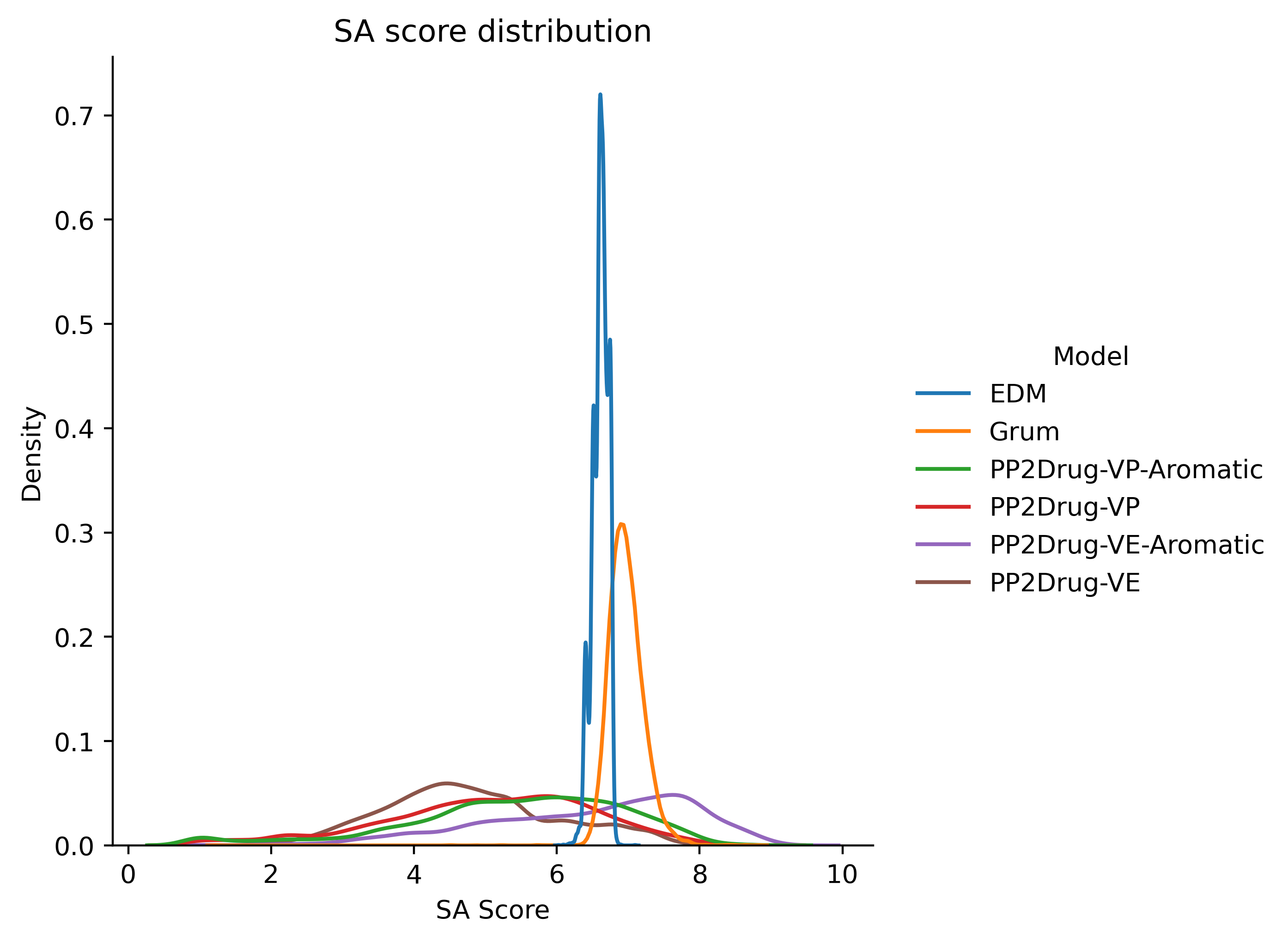
(a) Synthetic accessibility score distribution

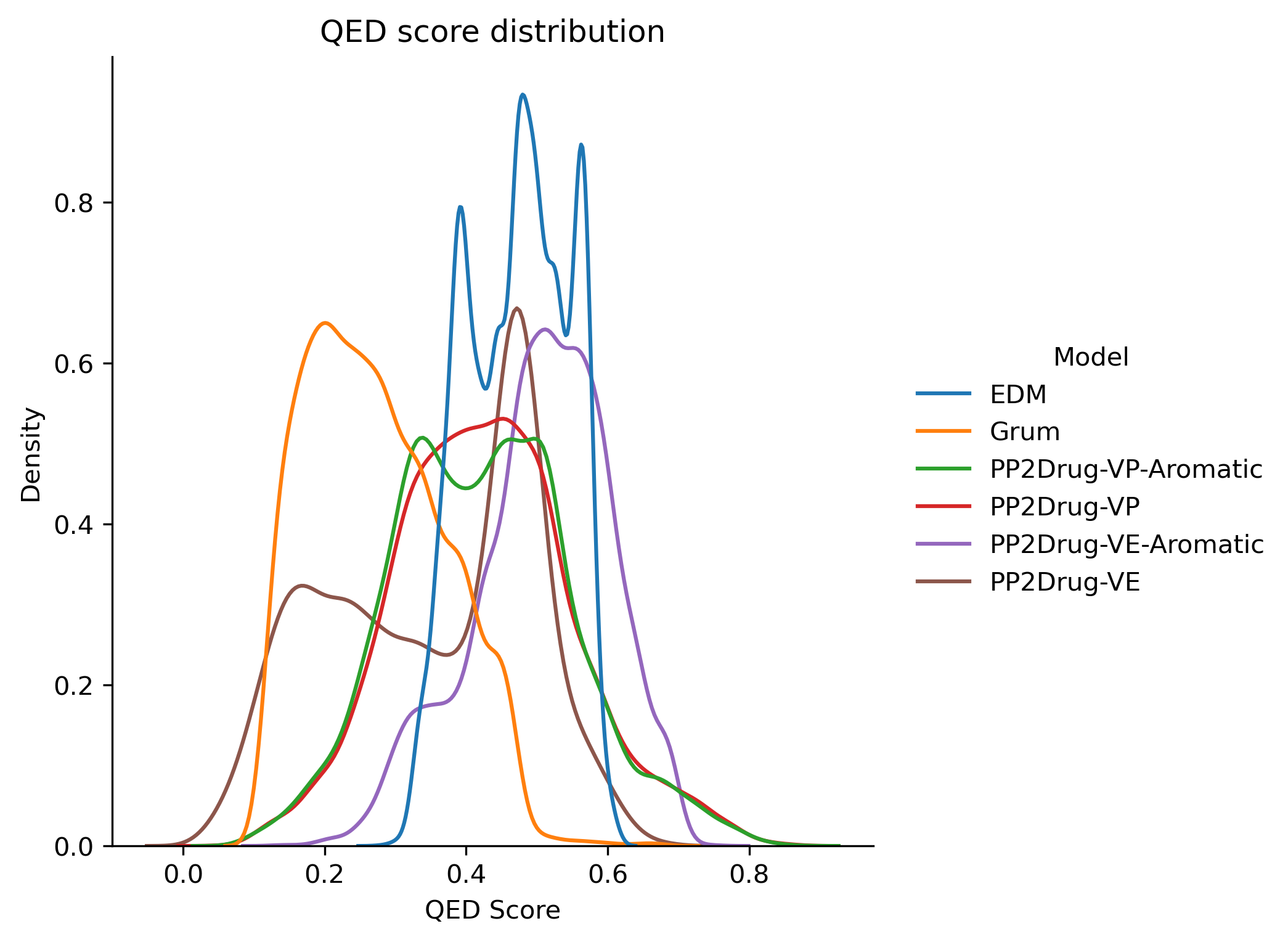
(b) Quantitative estimate of drug-likeness score distribution

Figure 3: SA and QED score distribution. Most of the samples generated by our model exhibit lower SA scores, indicating higher possibility of synthesis. For QED evaluation, except GruM and PP2Drug with VE bridge, other models are able to produce potential drug candidates.

Figure 3 presents the distribution of SA and QED scores of generated molecules. Our model generated molecules with evenly distributed SA scores, whereas SA scores of EDM and GruM generated molecules fell between 6.0 and 8.0. The majority of our samples achieved lower scores, indicating better synthetic accessibility. In the QED evaluation, GruM and VE-based PP2Drug obtained relatively lower scores while other models generated molecules with high drug-likeness.

In conclusion, PP2Drug achieved comparable validity, novelty and QED scores against state-of-the-art baselines and outperformed the baselines in terms of uniqueness and SA scores. In the ablation study, we found VE bridge-based PP2Drug was inclined to produce invalid chemical structures, whereas VP bridge-based PP2Drug exhibited better performance. This is aligned with the findings observed in previous works comparing VP and VE-based diffusion models [35, 17]. In addition, incorporating aromatic features brought slight improvement in uniqueness and novelty. We therefore continue the subsequent experiments with VP-based PP2Drug with aromatic features.

4.3 Pharmacophore-guided hit molecule design

We further demonstrate PP2Drug in pharmacophore-guided drug design tasks, including ligand-based drug design and structure-based drug design (SBDD).

4.3.1 Ligand-based drug design

Ligand-based drug design relies on knowledge of active molecules whose target structures remain obscure. By analyzing the chemical properties and structures of these ligands, we can create pharmacophore hypotheses to identify or design new compounds with similar or improved interactions. In order to assess our model in the ligand-based drug design task, we sample new molecules using the pharmacophore arrangements extracted from known active ligands. The pocket structure of each ligand’s receptor protein is utilized as constraint for sampling from Pocket2Mol and TargetDiff.

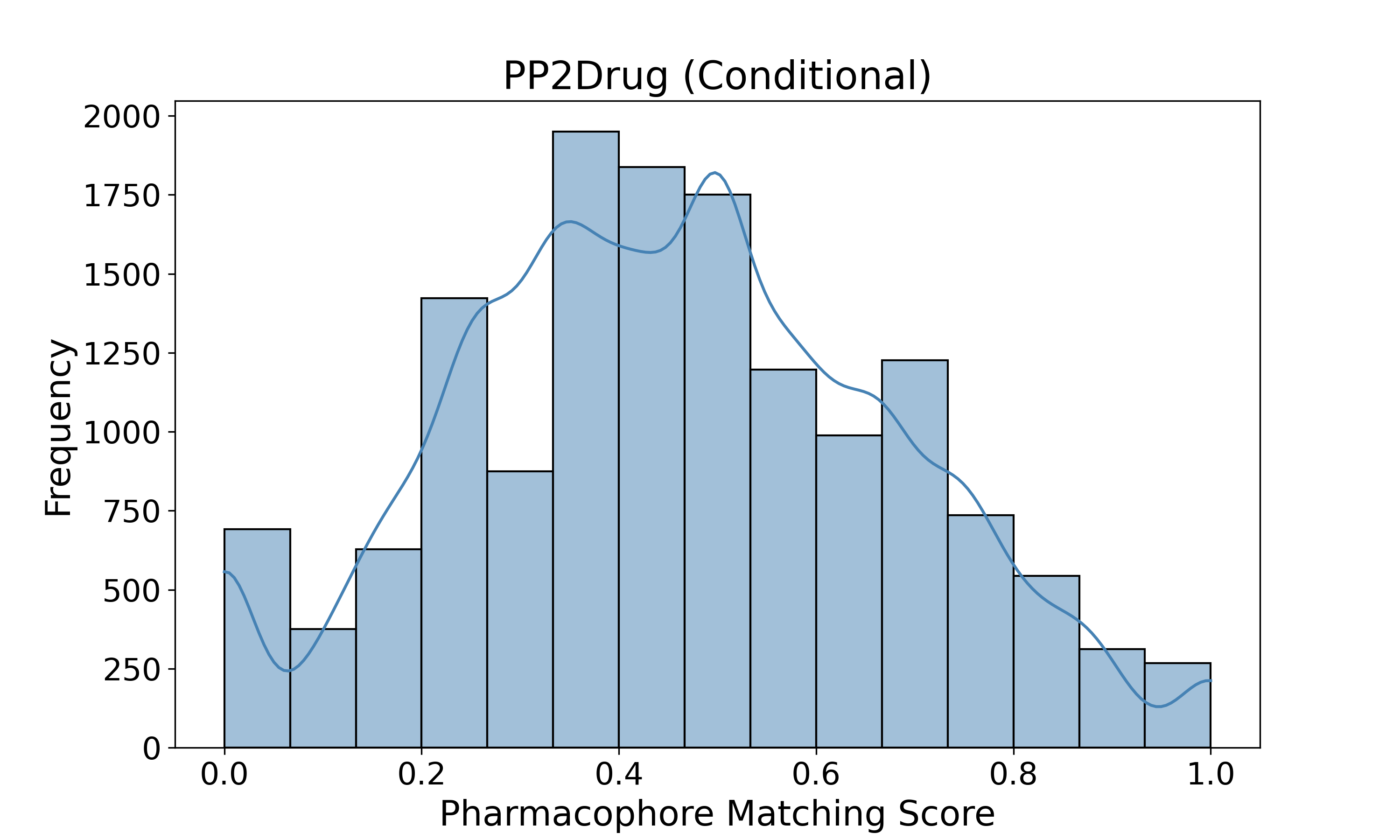
(a) Constrained PP2Drug

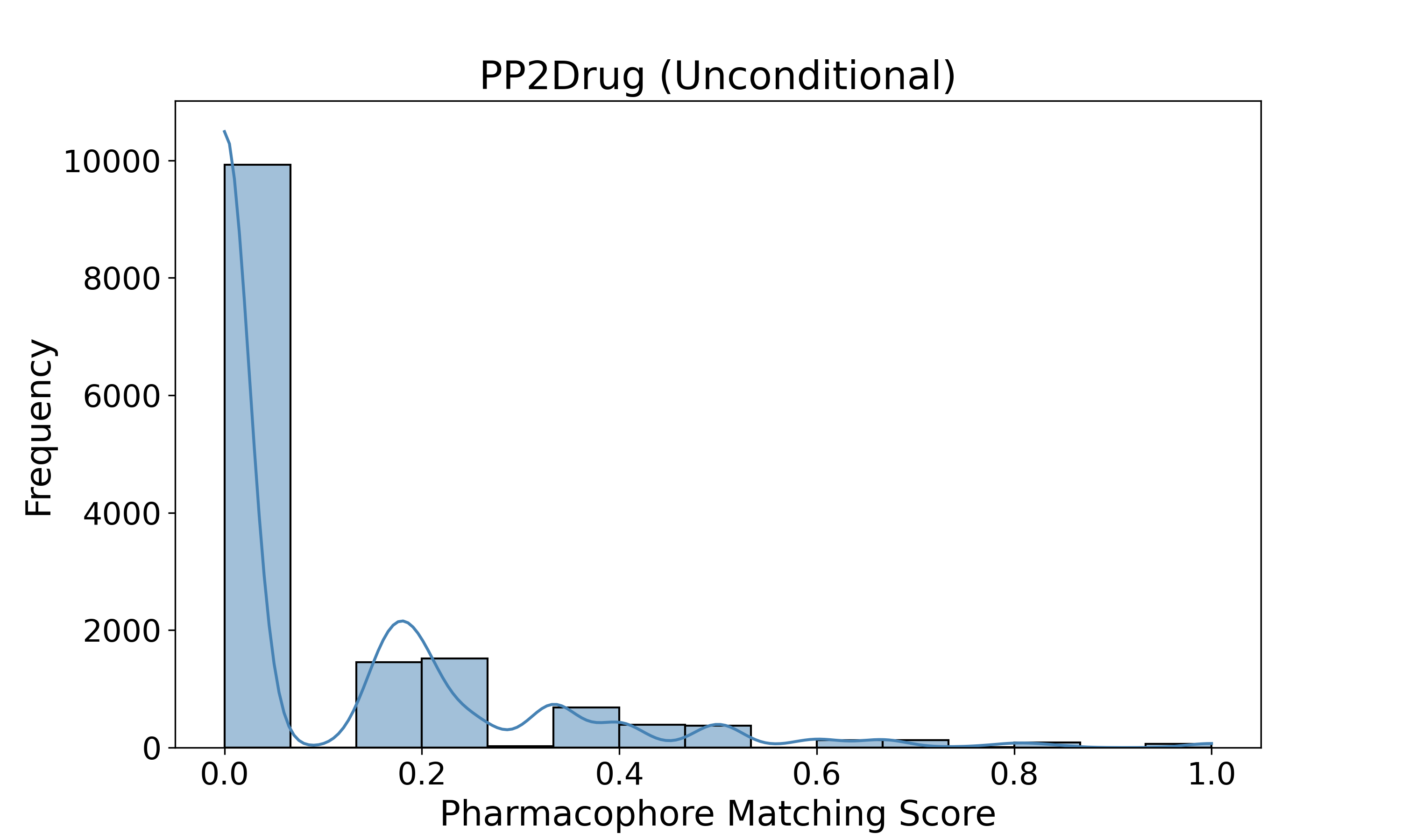
(b) Unconstrained PP2Drug

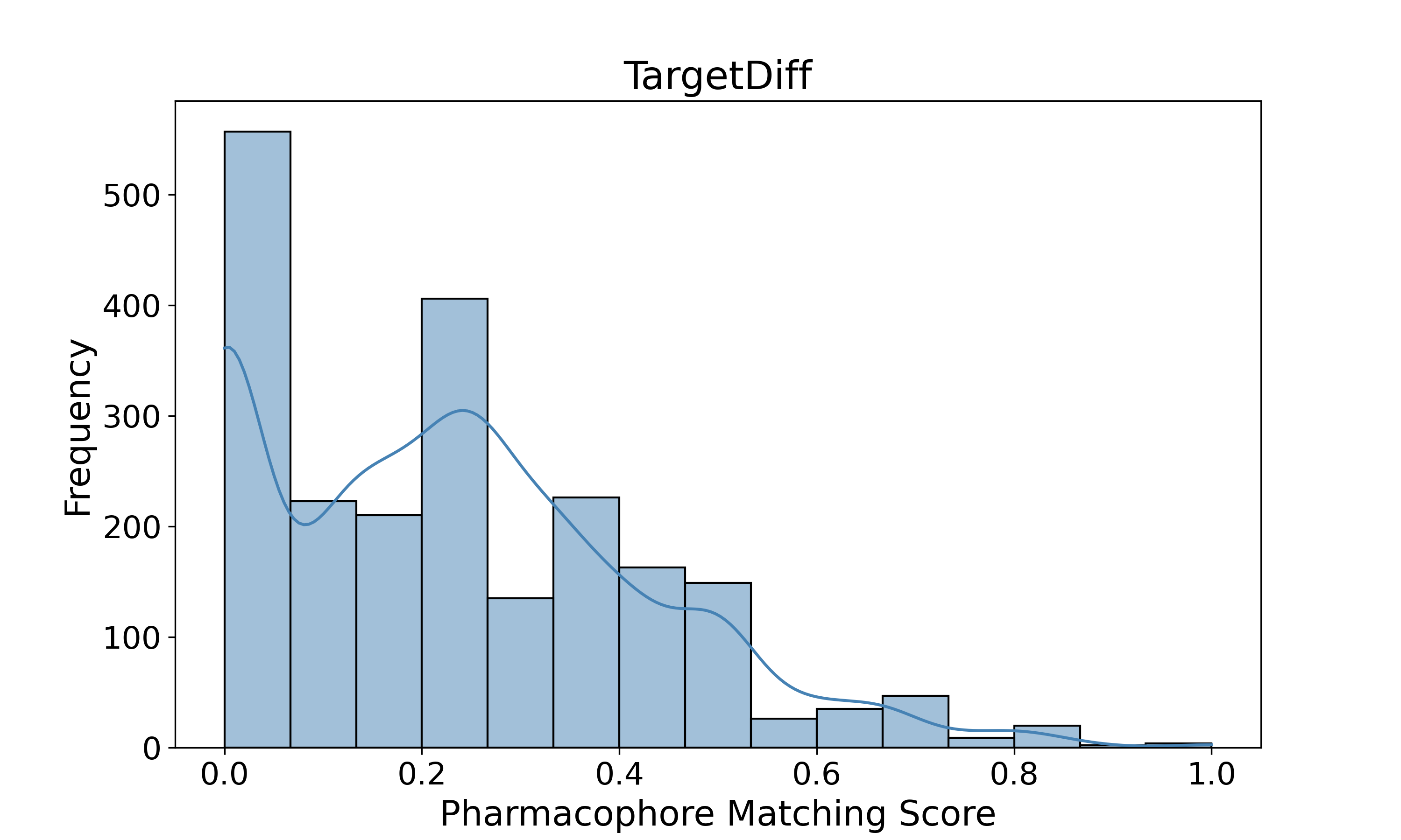
(c) TargetDiff

Figure 4: Pharmacophore matching sore distribution. Compared with Unconstrained generation and TargetDiff, pharmacophore-guided generation significantly enhanced the matching of pharmacophores extracted from original ligands and generated molecules. Notably, TargetDiff suffered from low validity, which resulting in less available molecules.

We extracted all pharmacophores of around 15k original ligands in the testing set, and removed the smaller groups that overlapped with the larger ones. New samples were generated by our model constrained by the extracted pharmacophores. We then computed the pharmacophore matching score reflecting the recovery rate of desired pharmacophore arrangements. Specifically, we calculated the distance between pharmacophores of generated molecules and original ligands. If the type of a pair of pharmacophores coincides and the distance is less than 1.5 Å, we consider this as a match. The matching score of each ligand is derived as $N_{match}/N_{pp}$, where $N_{match}$ and $N_{pp}$ represent number of matches and number of existing pharmacophores, respectively.

Figure 4 displays the histograms of pharmacophore matching scores. TargetDiff, which designs drugs directly constrained by pocket structures, were used as our baseline. Notably, only around two thousand molecules generated by TargetDiff were valid. Pocket2Mol was excluded from this assessment due to its limitation to autoregressive generation, without support for batch processing, which significantly prolongs the time required to generate approximately 15,000 samples. In addition, we included molecules generated by the unconditional version of our model as one of the baselines for comparison. As shown in Figure 4, PP2Drug significantly enhanced the pharmacophore recovery compared to unconstrained generation and TargetDiff. This suggests that the generated molecules have great potential to interact with the target protein, engaging not only within the desired pocket but also with the particular residue.

4.3.2 Structure-based drug design

SBDD, on the contrary to ligand-based drug design, utilizes the 3D structure of the target, typically a protein, to guide drug development. This method allows researchers to design molecules that fit precisely within the binding pocket of the target, optimizing interactions at an atomic level for enhanced efficacy and specificity.

We selected 10 protein targets, manually identified the essential pharmacophore features for the ligands to bind with each protein target, and generated 100 hit candidates guided by the identified pharmacophores. Firstly, we evaluated the matching scores by comparing the pharmacophore features used as constraints and the ones extracted from the generated molecules. The average matching scores of PP2Drug and baseline models are presented in Table 3. Our method achieved the highest average matching score in all cases.

Table 3: Average pharmacophore matching score of structure-based drug design.

PDB ID	PP2Drug	Pocket2Mol	TargetDiff
1EOC	0.76	0.34	0.17
5LSA	0.71	0.46	0.25
4H2Z	0.91	0.49	0.38
1J06	1.0	0.08	0.11
3OCC	0.74	0.22	0.24
5UEV	0.84	0.39	0.17
5FE6	1.0	0.45	0.23
5LPJ	0.83	0.41	0.17
5IJS	0.97	0.31	0.14
4TTI	0.98	0.37	0.20

Furthermore, we performed molecular docking analysis to demonstrate if the generated molecules are potential to interact with the protein targets. Gnina, a molecular docking software based on AutoDock Vina, was employed to test the binding affinity. Figure 5 shows the distribution of the Vina scores in box plots, with lower values representing higher binding affinities. The red dashed line in each group indicates the reference docking score of the original ligand provided by the CrossDocked dataset. It is evident that our method consistently generated molecules with higher binding affinities than the original ligand across each group. Pocket2Mol sometimes outperformed our method, but the generated molecules exhibited significantly wide range of Vina scores, especially in cases of 1EOC and 4H2Z, rendering this approach very unstable. TargetDiff achieved the worst performance with most of the generated molecules gaining higher Vina scores than the reference ligand.

In addition, percentage of generated molecules with higher binding affinity are calculated and shown in Table 4, together with the number of available samples and the reference Vina score. It is evident that PP2Drug is able to produce hit candidates with over 90% higher binding affinities in most cases. Pocket2Mol are competitive in certain groups such as 1J06, 3OCC, 5UEV, 5FE6 and 5IJS, but produces only around 50% of higher affinity samples in the other groups. TargetDiff, however, are limited by a low validity rate. We present example molecules generated by PP2Drug using the pharmacophores identified in the binding complex structures of 1EOC, 3OCC and 5UEV in Figure 6, including both 3D docked binding complexes and 2D chemical structures.

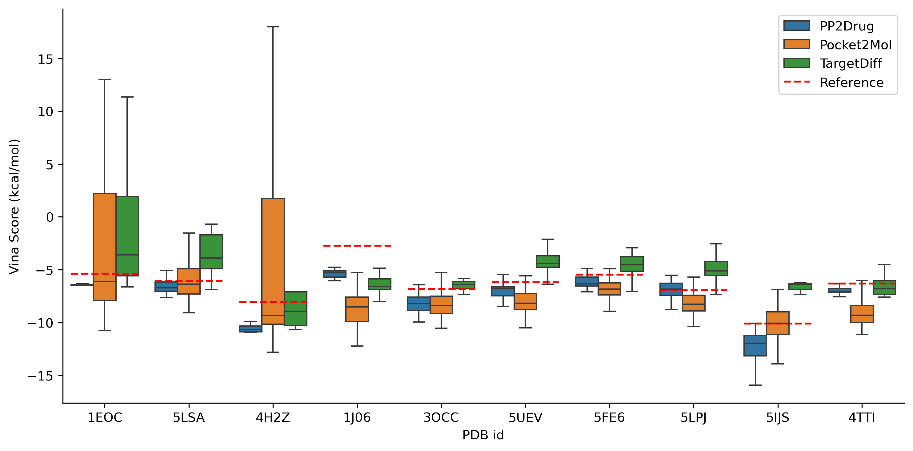
Figure 5: Distribution of Vina docking scores, with lower vina score representing higher binding affinity. The reference scores given by the original ligands are indicated by red dashed lines in the figure. PP2Drug consistently generated molecules with higher binding affinities. Although Pocket2Mol sometimes outperformed, it produced molecules with a notably broad range of Vina scores in certain groups, e.g., 1EOC and 4H2Z. TargetDiff failed to generate molecules with binding affinities surpassing those of the original ligands in most cases.

Table 4: Percentage of generated molecules with higher binding affinity.

PDB ID	PP2Drug		Pocket2Mol		TargetDiff		Reference score
	High affinity ratio (%)	Sample num	High affinity ratio (%)	Sample num	High affinity ratio (%)	Sample num	(kcal/mol)
1EOC	99.00	100	55.34	100	30.00	10	-5.39
5LSA	76.00	100	52.78	100	3.70	28	-6.06
4H2Z	100.00	100	57.69	100	55.56	9	-8.06
1J06	100.00	100	98.15	100	100.00	16	-2.73
3OCC	93.00	100	91.51	100	25.00	8	-6.84
5UEV	91.00	100	94.87	100	8.89	45	-6.20
5FE6	80.00	100	90.99	100	18.75	32	-5.46
5LPJ	48.00	100	83.02	100	10.00	20	-6.95
5IJS	98.99	99	48.54	100	0.00	3	-10.11
4TTI	99.00	100	91.18	100	66.57	12	-6.32

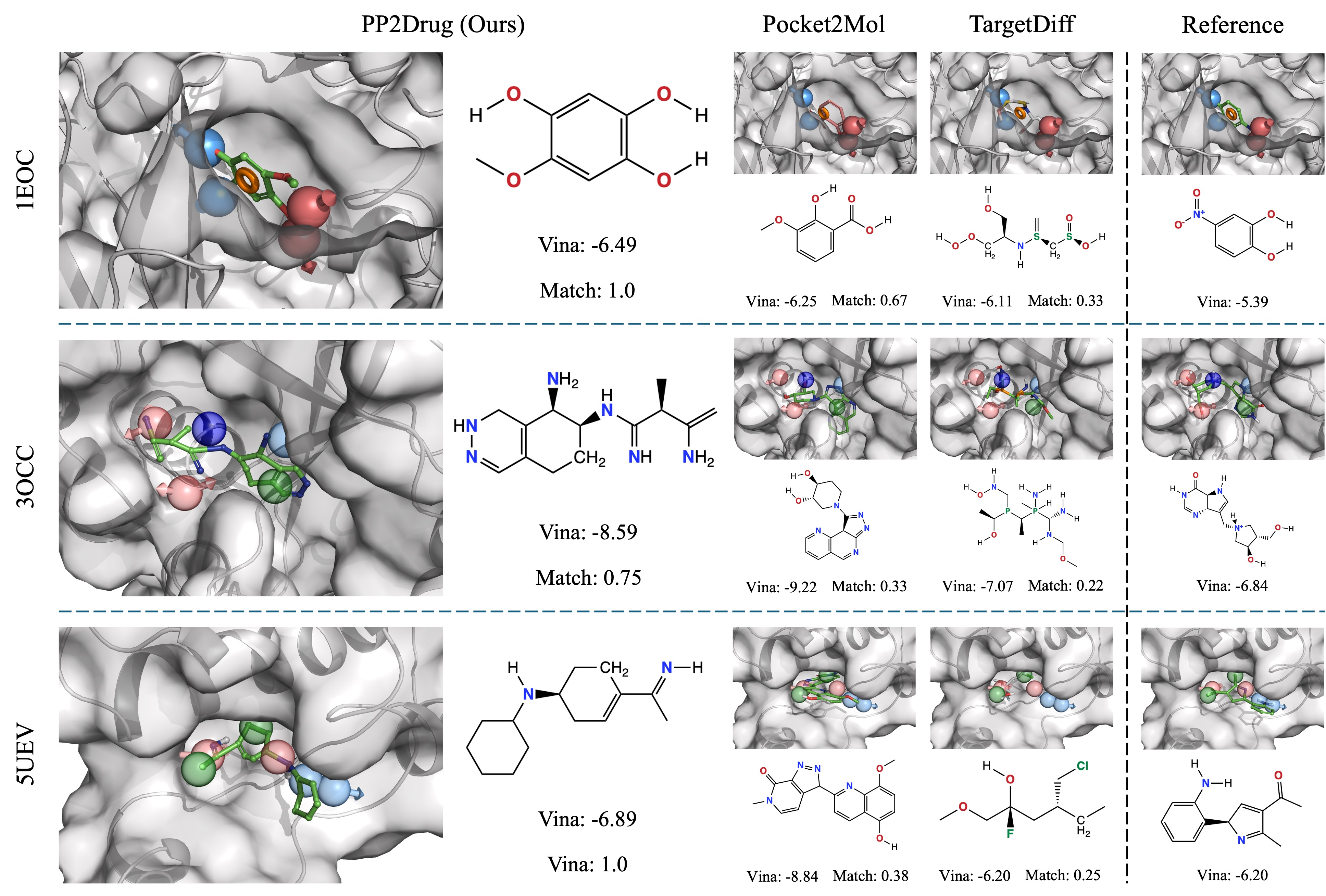
Figure 6: Molecules generated with the pharmacophore models of ligands from PDB structure 5JOY, 4CPI, 1DOD. Docked binding complexes and chemical structures, together with the Vina and CNN scores of both generated and original molecules are shown.

5 Conclusion

In this work, we presented PP2Drug - a diffusion bridge model designed for graph translation. Bridge processes enable us to construct a transitional probability flow between any two distributions and the idea of diffusion model makes such transition kernel tractable. We proposed a practical solution to leverage such models for graph generation constrained by the cluster arrangements of nodes, and demonstrated our model on the task of pharmacophore-guided de novo hit molecule design. We parameterized our denoiser with $E(3)$-equivariant GNN. Constrained by the pharmacophore models extracted from the active ligands, our model managed to generate potential hit candidates with higher binding affinity with the receptor of the original ligands.

References

- [1] Olivier J Wouters, Martin McKee, and Jeroen Luyten. Estimated research and development investment needed to bring a new medicine to market, 2009-2018. Jama, 323(9):844–853, 2020.
- [2] Joshua Meyers, Benedek Fabian, and Nathan Brown. De novo molecular design and generative models. Drug discovery today, 26(11):2707–2715, 2021.
- [3] Diederik P Kingma and Max Welling. Auto-encoding variational bayes. arXiv preprint arXiv:1312.6114, 2013.
- [4] Ian Goodfellow, Jean Pouget-Abadie, Mehdi Mirza, Bing Xu, David Warde-Farley, Sherjil Ozair, Aaron Courville, and Yoshua Bengio. Generative adversarial networks. Communications of the ACM, 63(11):139–144, 2020.
- [5] Jonathan Ho, Ajay Jain, and Pieter Abbeel. Denoising diffusion probabilistic models. Advances in Neural Information Processing Systems, 33:6840–6851, 2020.
- [6] David Weininger. Smiles, a chemical language and information system. 1. introduction to methodology and encoding rules. Journal of chemical information and computer sciences, 28(1):31–36, 1988.
- [7] Oleksii Prykhodko, Simon Viet Johansson, Panagiotis-Christos Kotsias, Josep Arús-Pous, Esben Jannik Bjerrum, Ola Engkvist, and Hongming Chen. A de novo molecular generation method using latent vector based generative adversarial network. Journal of Cheminformatics, 11:1–13, 2019.
- [8] Oscar Méndez-Lucio, Benoit Baillif, Djork-Arné Clevert, David Rouquié, and Joerg Wichard. De novo generation of hit-like molecules from gene expression signatures using artificial intelligence. Nature communications, 11(1):10, 2020.
- [9] Jannis Born, Matteo Manica, Ali Oskooei, Joris Cadow, Greta Markert, and María Rodríguez Martínez. Paccmannrl: De novo generation of hit-like anticancer molecules from transcriptomic data via reinforcement learning. Iscience, 24(4), 2021.
- [10] Kazuma Kaitoh and Yoshihiro Yamanishi. Triomphe: Transcriptome-based inference and generation of molecules with desired phenotypes by machine learning. Journal of Chemical Information and Modeling, 61(9):4303–4320, 2021.
- [11] Martin Simonovsky and Nikos Komodakis. Graphvae: Towards generation of small graphs using variational autoencoders. In Artificial Neural Networks and Machine Learning–ICANN 2018: 27th International Conference on Artificial Neural Networks, Rhodes, Greece, October 4-7, 2018, Proceedings, Part I 27, pages 412–422. Springer, 2018.
- [12] Nicola De Cao and Thomas Kipf. Molgan: An implicit generative model for small molecular graphs. arXiv preprint arXiv:1805.11973, 2018.
- [13] Chengxi Zang and Fei Wang. Moflow: an invertible flow model for generating molecular graphs. In Proceedings of the 26th ACM SIGKDD international conference on knowledge discovery & data mining, pages 617–626, 2020.
- [14] Chence Shi, Minkai Xu, Zhaocheng Zhu, Weinan Zhang, Ming Zhang, and Jian Tang. Graphaf: a flow-based autoregressive model for molecular graph generation. arXiv preprint arXiv:2001.09382, 2020.
- [15] Krzysztof Maziarz, Henry Jackson-Flux, Pashmina Cameron, Finton Sirockin, Nadine Schneider, Nikolaus Stiefl, Marwin Segler, and Marc Brockschmidt. Learning to extend molecular scaffolds with structural motifs. arXiv preprint arXiv:2103.03864, 2021.
- [16] Zaixi Zhang, Qi Liu, Hao Wang, Chengqiang Lu, and Chee-Kong Lee. Motif-based graph self-supervised learning for molecular property prediction. Advances in Neural Information Processing Systems, 34:15870–15882, 2021.
- [17] Yang Song, Jascha Sohl-Dickstein, Diederik P Kingma, Abhishek Kumar, Stefano Ermon, and Ben Poole. Score-based generative modeling through stochastic differential equations. arXiv preprint arXiv:2011.13456, 2020.
- [18] Robin Rombach, Andreas Blattmann, Dominik Lorenz, Patrick Esser, and Björn Ommer. High-resolution image synthesis with latent diffusion models. In Proceedings of the IEEE/CVF conference on computer vision and pattern recognition, pages 10684–10695, 2022.
- [19] Clement Vignac, Igor Krawczuk, Antoine Siraudin, Bohan Wang, Volkan Cevher, and Pascal Frossard. Digress: Discrete denoising diffusion for graph generation. arXiv preprint arXiv:2209.14734, 2022.
- [20] Jaehyeong Jo, Seul Lee, and Sung Ju Hwang. Score-based generative modeling of graphs via the system of stochastic differential equations. In International Conference on Machine Learning, pages 10362–10383. PMLR, 2022.
- [21] Haitao Lin, Yufei Huang, Odin Zhang, Yunfan Liu, Lirong Wu, Siyuan Li, Zhiyuan Chen, and Stan Z Li. Functional-group-based diffusion for pocket-specific molecule generation and elaboration. Advances in Neural Information Processing Systems, 36, 2024.
- [22] Minkai Xu, Lantao Yu, Yang Song, Chence Shi, Stefano Ermon, and Jian Tang. Geodiff: A geometric diffusion model for molecular conformation generation. arXiv preprint arXiv:2203.02923, 2022.
- [23] Minkai Xu, Alexander S Powers, Ron O Dror, Stefano Ermon, and Jure Leskovec. Geometric latent diffusion models for 3d molecule generation. In International Conference on Machine Learning, pages 38592–38610. PMLR, 2023.
- [24] Arne Schneuing, Yuanqi Du, Charles Harris, Arian Jamasb, Ilia Igashov, Weitao Du, Tom Blundell, Pietro Lió, Carla Gomes, Max Welling, et al. Structure-based drug design with equivariant diffusion models. arXiv preprint arXiv:2210.13695, 2022.
- [25] Emiel Hoogeboom, Vıctor Garcia Satorras, Clément Vignac, and Max Welling. Equivariant diffusion for molecule generation in 3d. In International conference on machine learning, pages 8867–8887. PMLR, 2022.
- [26] Jiaqi Guan, Wesley Wei Qian, Xingang Peng, Yufeng Su, Jian Peng, and Jianzhu Ma. 3d equivariant diffusion for target-aware molecule generation and affinity prediction. arXiv preprint arXiv:2303.03543, 2023.
- [27] Yang Song and Stefano Ermon. Generative modeling by estimating gradients of the data distribution. Advances in neural information processing systems, 32, 2019.
- [28] Xingchao Liu, Lemeng Wu, Mao Ye, and Qiang Liu. Let us build bridges: Understanding and extending diffusion generative models. arXiv preprint arXiv:2208.14699, 2022.
- [29] Mao Ye, Lemeng Wu, and Qiang Liu. First hitting diffusion models for generating manifold, graph and categorical data. Advances in Neural Information Processing Systems, 35:27280–27292, 2022.
- [30] Joseph L Doob and JI Doob. Classical potential theory and its probabilistic counterpart, volume 262. Springer, 1984.
- [31] Tianrong Chen, Guan-Horng Liu, and Evangelos A Theodorou. Likelihood training of schr" odinger bridge using forward-backward sdes theory. arXiv preprint arXiv:2110.11291, 2021.
- [32] Francisco Vargas, Pierre Thodoroff, Austen Lamacraft, and Neil Lawrence. Solving schrödinger bridges via maximum likelihood. Entropy, 23(9):1134, 2021.
- [33] Gefei Wang, Yuling Jiao, Qian Xu, Yang Wang, and Can Yang. Deep generative learning via schrödinger bridge. In International conference on machine learning, pages 10794–10804. PMLR, 2021.
- [34] Xuan Su, Jiaming Song, Chenlin Meng, and Stefano Ermon. Dual diffusion implicit bridges for image-to-image translation. arXiv preprint arXiv:2203.08382, 2022.
- [35] Linqi Zhou, Aaron Lou, Samar Khanna, and Stefano Ermon. Denoising diffusion bridge models. arXiv preprint arXiv:2309.16948, 2023.
- [36] Lemeng Wu, Chengyue Gong, Xingchao Liu, Mao Ye, and Qiang Liu. Diffusion-based molecule generation with informative prior bridges. Advances in Neural Information Processing Systems, 35:36533–36545, 2022.
- [37] Jaehyeong Jo, Dongki Kim, and Sung Ju Hwang. Graph generation with diffusion mixture. arXiv preprint arXiv:2302.03596, 2023.
- [38] Vignesh Ram Somnath, Matteo Pariset, Ya-Ping Hsieh, Maria Rodriguez Martinez, Andreas Krause, and Charlotte Bunne. Aligned diffusion schrödinger bridges. In Uncertainty in Artificial Intelligence, pages 1985–1995. PMLR, 2023.
- [39] Conghao Wang, Hiok Hian Ong, Shunsuke Chiba, and Jagath C Rajapakse. Gldm: hit molecule generation with constrained graph latent diffusion model. Briefings in Bioinformatics, 25(3):bbae142, 2024.
- [40] Xingang Peng, Shitong Luo, Jiaqi Guan, Qi Xie, Jian Peng, and Jianzhu Ma. Pocket2mol: Efficient molecular sampling based on 3d protein pockets. In International Conference on Machine Learning, pages 17644–17655. PMLR, 2022.
- [41] Seonghwan Seo and Woo Youn Kim. Pharmaconet: Accelerating structure-based virtual screening by pharmacophore modeling. arXiv preprint arXiv:2310.00681, 2023.
- [42] Huimin Zhu, Renyi Zhou, Dongsheng Cao, Jing Tang, and Min Li. A pharmacophore-guided deep learning approach for bioactive molecular generation. Nature Communications, 14(1):6234, 2023.
- [43] Tero Karras, Miika Aittala, Timo Aila, and Samuli Laine. Elucidating the design space of diffusion-based generative models. Advances in Neural Information Processing Systems, 35:26565–26577, 2022.
- [44] Vıctor Garcia Satorras, Emiel Hoogeboom, and Max Welling. E (n) equivariant graph neural networks. In International conference on machine learning, pages 9323–9332. PMLR, 2021.
- [45] Paul G Francoeur, Tomohide Masuda, Jocelyn Sunseri, Andrew Jia, Richard B Iovanisci, Ian Snyder, and David R Koes. Three-dimensional convolutional neural networks and a cross-docked data set for structure-based drug design. Journal of chemical information and modeling, 60(9):4200–4215, 2020.