\newsiamremark

remarkRemark \newsiamremarkhypothesisHypothesis \newsiamthmclaimClaim \headersLévy Score and Score-Based Particle AlgorithmY. HUANG, C. LIU and X. ZHOU

Lévy Score Function and Score-Based Particle Algorithm for Nonlinear Lévy–Fokker–Planck Equationsthanks: Submitted to the editors DATE. \fundingThis work was funded by the Hong Kong General Research Funds (11308121, 11318522, 11308323), and the NSFC/RGC Joint Research Scheme [RGC Project No. N-CityU102/20 and NSFC Project No. 12061160462.

Yuanfei Huang Department of Data Science, City University of Hong Kong, Kowloon, Hong Kong SAR, (). yhuan26@cityu.edu.hk    Chengyu Liu Department of Data Science, City University of Hong Kong, Kowloon, Hong Kong SAR, (). cliu687-c@my.cityu.edu.hk    Xiang Zhou Department of Mathematics, City University of Hong Kong, Kowloon, Hong Kong SAR, () xizhou@cityu.edu.hk
Abstract

The score function for the diffusion process, also known as the gradient of the log-density, is a basic concept to characterize the probability flow with important applications in the score-based diffusion generative modelling and the simulation of Itô stochastic differential equations. However, neither the probability flow nor the corresponding score function for the diffusion-jump process are known. This paper delivers mathematical derivation, numerical algorithm, and error analysis focusing on the corresponding score function in non-Gaussian systems with jumps and discontinuities represented by the nonlinear Lévy–Fokker–Planck equations. We propose the Lévy score function for such stochastic equations, which features a nonlocal double-integral term, and we develop its training algorithm by minimizing the proposed loss function from samples. Based on the equivalence of the probability flow with deterministic dynamics, we develop a self-consistent score-based transport particle algorithm to sample the interactive Lévy stochastic process at discrete time grid points. We provide error bound for the Kullback–Leibler divergence between the numerical and true probability density functions by overcoming the nonlocal challenges in the Lévy score. The full error analysis with the Monte Carlo error and the time discretization error is furthermore established. To show the usefulness and efficiency of our approach, numerical examples from applications in biology and finance are tested.

keywords:
score function; stochastic differential equation; Lévy–Fokker–Planck equation; probability flow; score-based particle method; Lévy noise.
{MSCcodes}

65M75, 65C35, 68T07, 60H35

1 Introduction

Stochastic processes, such as the Itô diffusion process and the Lévy jump process, play prominent roles in a variety range of fields including science, engineering, economics, and statistics. The temporal evolution of the probability distribution, satisfying the initial-value forward Kolmogorov equation, can be also viewed as a path or curve in the space of probability distributions. The path connecting two probability density functions associated certain stochastic processes is the crucial mathematical tool the basis of score-based generative algorithms [38].

The viewpoint of probability flow is to treat the time evolution of the probability density function as the continuity equation whose velocity field contains the gradient of the density function in the self-consistent way. In the setting of a diffusion process Xtsubscript𝑋𝑡X_{t}, the density function ptsubscript𝑝𝑡p_{t} of Xtsubscript𝑋𝑡X_{t} is given by the Fokker-Planck equation

(1) pt(x)t=subscript𝑝𝑡𝑥𝑡absent\displaystyle\frac{\partial p_{t}(x)}{\partial t}= [(b(x,t)12Σ(x,t)12Σ(x,t)logpt(x))v(x,t)pt(x)],delimited-[]subscript𝑏𝑥𝑡12Σ𝑥𝑡12Σ𝑥𝑡subscript𝑝𝑡𝑥𝑣𝑥𝑡subscript𝑝𝑡𝑥\displaystyle\ -\nabla\cdot\left[\underbrace{\left(b(x,t)-\frac{1}{2}\nabla\cdot\Sigma(x,t)-\frac{1}{2}\Sigma(x,t)\nabla\log p_{t}(x)\right)}_{v(x,t)}p_{t}(x)\right],

where b𝑏b is the drift term and ΣΣ\Sigma corresponds to the diffusion matrix. If the term logptsubscript𝑝𝑡\nabla\log p_{t}, denoted by the score function st(x)subscript𝑠𝑡𝑥s_{t}(x), is known a prior, then (1) takes the form of a continuity equation corresponds to the transportation between the density functions p0subscript𝑝0p_{0} and pTsubscript𝑝𝑇p_{T} by a underlying deterministic ODE flow with the new vector field v(x,t):=b(x,t)1/2Σ(x,t)1/2Σ(x,t)st(x)assign𝑣𝑥𝑡𝑏𝑥𝑡12Σ𝑥𝑡12Σ𝑥𝑡subscript𝑠𝑡𝑥v(x,t):=b(x,t)-1/2\nabla\cdot\Sigma(x,t)-1/2\Sigma(x,t)s_{t}(x). This observation is also the theoretic foundation of reversing a Markov diffusion process in score-based diffusion models since the time reverse from pTsubscript𝑝𝑇p_{T} to p0subscript𝑝0p_{0} can implemented by the time-reversed deterministic flow. However, the various numerical methods [19, 36, 38, 34] to find the score function stsubscript𝑠𝑡s_{t} for the generative modeling like image synthesis are limited to the constant drift or the Orenstein-Ulenbeck process, because these simple processes suffice to inject Gaussian noise to the data. In such simple systems, the transition probability is analytically available.

Motivated by the probability flow and score-based generative models, a number of studies [29, 33, 24, 28, 4, 32] have been recently carried out to learn the underlying velocity field v(x,t)𝑣𝑥𝑡v(x,t) that drives the probability density function in Fokker-Planck equations, instead of directly simulating the diffusion SDE or solving the Fokker-Planck PDE. These methods, usually referred to as score-based transport modeling[4], deterministically push samples from the initial density onto samples from the solution at any later time by employing particle methods to learn the score function from the samples following the deterministic flow. By finding the above mentioned score function appearing in the new velocity field, this numerical strategy works well due to the self-consistency of the Fokker-Planck equation [24, 24] in the form of fixed-point argument. Compared with the traditional grid-based numerical methods for the Fokker–Planck equation, these score-based methods can scale well in high dimensions. Compared to the traditional numerical SDE schemes, the deterministic flow is faster to compute and offers the expression of the density function to facilitate calculating many non-equilibrium statistical quantities like the probability current, the entropy production rate and the heat [39, 5]. The theoretic works related to these algorithms include the error analysis for Kullback-Leibler divergence due to the approximate score function [32, 33, 28, 4]. There are also substantial extensions from the Fokker-Planck equation to the McKean-Vlaso equation [29, 32, 28] and the Fokker-Planck-Landau equation[20, 17].

However, the existing score-based transport modeling only studied the diffusion process with the focus on the conventional score function st=logptsubscript𝑠𝑡subscript𝑝𝑡s_{t}=\nabla\log p_{t} and the score matching error t0TΩ|sθ(x,t)logpt(x)|2pt(x)dxdtsuperscriptsubscriptsubscript𝑡0𝑇subscriptΩsuperscriptsuperscript𝑠𝜃𝑥𝑡subscript𝑝𝑡𝑥2subscript𝑝𝑡𝑥differential-d𝑥differential-d𝑡\int_{t_{0}}^{T}\int_{\Omega}|s^{\theta}(x,t)-\nabla\log p_{t}(x)|^{2}p_{t}(x)\,\mathrm{d}x\,\mathrm{d}t as the loss function to train the score. Despite the popularity in applications of the diffusion model, the non-Gaussian processes such as Lévy processes are preferred to more accurately represent complex stochastic events than conventional Gaussian models [22, 3, 35]. Recently, the Lévy-Itô model with the fractional score function st(α)(x)=(α22pt(x))/pt(x)superscriptsubscript𝑠𝑡𝛼𝑥superscript𝛼22subscript𝑝𝑡𝑥subscript𝑝𝑡𝑥s_{t}^{(\alpha)}(x)=(\triangle^{\frac{\alpha-2}{2}}\nabla p_{t}(x))/p_{t}(x), α(1,2]𝛼12\alpha\in(1,2], is used in [41] for score-based generative models to generate more diverse samples by taking advantage of the heavy-tailed properties of the α𝛼\alpha-stable Lévy process. In [16], the same fractional score function is computed for the Lévy–Fokker–Planck equation by training the fractional score-based physics-informed neural networks from a large number of sample stochastic trajectories as the training data.

In this paper, we systematically investigate the score-based transport modeling for the general Markov process of non-Gaussian type and develop the score-based theories and algorithms to simulate the underlying jump-diffusion process. This paper delivers mathematical derivation, numerical algorithm, and error analysis focusing on the corresponding score function in non-Gaussian systems with jumps and discontinuities represented by the nonlinear Lévy–Fokker–Planck equations. We propose the Lévy score function for such stochastic equations, which features a nonlocal double-integral term, and its training algorithm by minimizing the proposed loss function from samples. Based on the equivalence of the probability flow with deterministic dynamics, we develop a self-consistent score-based transport particle algorithm to sample the interactive Lévy stochastic process at discrete time grid points.

Contributions

  1. 1.

    For the nonlinear stochastic differential equation (2) driven by the Brownian and Lévy noise as well as the mean-field interaction, we derive the continuity equation for the nonlinear Lévy-Fokker-Planck equation (4) to identify the vector field in the probability flow. We propose the generalized score function, S^tsubscript^𝑆𝑡\widehat{S}_{t} in (8), consisting of both the conventional diffusion score function logptsubscript𝑝𝑡\nabla\log p_{t} and the Lévy score function. The latter has the non-local double-integral terms involving the Lévy measure.

  2. 2.

    We show in Theorem 3.2 that, the Kullback–Leibler divergence supt[t0,T]DKL(ptθp^t)subscriptsupremum𝑡subscript𝑡0𝑇subscript𝐷KLconditionalsubscriptsuperscript𝑝𝜃𝑡subscript^𝑝𝑡\sup_{t\in[t_{0},T]}D_{\mathrm{KL}}(p^{\theta}_{t}\|\widehat{p}_{t}) between the numerical score-based ptθsubscriptsuperscript𝑝𝜃𝑡p^{\theta}_{t} and the true density function p^tsubscript^𝑝𝑡\widehat{p}_{t} is bounded by a loss function we derived from the fixed-point argument. This is a significant extension to [32, 33, 4, 28] since our analysis takes into account of both the non-Gaussian process and the mean-field interactions.

  3. 3.

    We propose the score-matching training algorithm to learn both the diffusion and Lévy score functions by one single neural network, then develop the sequential score-based particle algorithm (Algorithm 1) to solve the Lévy–Fokker–Planck equation based on the idea of score-based transport modeling. We test several numerical examples to demonstrate the effectiveness of our approach.

  4. 4.

    We prove in Theorem 3.4 the numerical error of Algorithm 1 for solving (2): 1T𝔼|XnΔtXnΔtN|𝒪(1N)+𝒪(ε)+𝒪(Δt),1𝑇𝔼subscriptsuperscript𝑋𝑛Δ𝑡subscriptsuperscript𝑋𝑁𝑛Δ𝑡𝒪1𝑁𝒪𝜀𝒪Δ𝑡\frac{1}{T}\mathbb{E}\left|X^{*}_{n\Delta t}-X^{N}_{n\Delta t}\right|\leq\mathcal{O}\left(\frac{1}{\sqrt{N}}\right)+\mathcal{O}(\varepsilon)+\mathcal{O}(\Delta t), with N𝑁N the number of particles, ϵitalic-ϵ\epsilon the bounds of score loss, and ΔtΔ𝑡\Delta t the time step size, nΔtT𝑛Δ𝑡𝑇n\Delta t\leq T.

Related works:

Score-based diffusion model and the error analysis. The score-based diffusion model is formulated as the forward and backward continuous Itô stochastic differential equations in [38]. The score matching to train the score function by neural networks includes [19, 37, 15, 34, 14, 27]. For comprehensive reviews on related topics, we refer readers to [12]. There are also extensive works to analyze the convergence and error estimates, for instance [10, 8, 7].

Score-based transport modeling for Fokker-Planck equation. These  methods are all based on (1) – the equivalence to probability flow – to simulate the time evolution of Fokker–Planck solutions. [29] runs a large number of interacting deterministic particles where the gradient–log–density (score) function is approximated in the reproducing kernel Hilbert space (RKHS). [33, 32] formulated a fixed-point problem for the self-consistency of the probability flow for the Fokker–Planck equation, but the optimization for the diffusion score function is based on the adjoint method which is in general slow and challenging to implement. The score-based transport modeling in [4] is to march the flow sequentially in time with the forward Euler scheme. Instead, [24] proposed to learn the velocity field v(t,x)𝑣𝑡𝑥v(t,x) as a whole for t[0,T]𝑡0𝑇t\in[0,T] by an iterative update of the velocity field.

Score-based generative models with α𝛼\alpha-stable Lévy processes. [41] proposed score-based generative models with a simple forward Lévy process Xt=a(t)X0+γ(t)ϵsubscript𝑋𝑡𝑎𝑡subscript𝑋0𝛾𝑡italic-ϵX_{t}=a(t)X_{0}+\gamma(t)\epsilon, where X0subscript𝑋0X_{0} follows the data distribution, and the noise ϵitalic-ϵ\epsilon follows the isotropic α𝛼\alpha-stable distribution with the scalar parameter 111. The fractional score function st(α)(x)=(α22pt(x))/pt(x)superscriptsubscript𝑠𝑡𝛼𝑥superscript𝛼22subscript𝑝𝑡𝑥subscript𝑝𝑡𝑥s_{t}^{(\alpha)}(x)=(\triangle^{\frac{\alpha-2}{2}}\nabla p_{t}(x))/p_{t}(x) with 1<α21𝛼21<\alpha\leq 2, is proposed for the pdf pt(x)subscript𝑝𝑡𝑥p_{t}(x) in order to define the time-reversal Lévy process. This fractional score function is approximated by a neural network and simple enough to use the denoising score-matching similarly to the score-based diffusion models.

Fractional score-based physics-informed neural networks(PINN) for α𝛼\alpha-stable Lévy processes . [16] proposed the score-fPINN method for the log-likelihood qt:=logptassignsubscript𝑞𝑡subscript𝑝𝑡q_{t}:=\log p_{t} of an α𝛼\alpha-stable Lévy process by minimizing the PINN loss for the two nonlinear PDEs of qtsubscript𝑞𝑡q_{t} and st=qtsubscript𝑠𝑡subscript𝑞𝑡s_{t}=\nabla q_{t} respectively, which involve the pairs q𝑞q and s(α)superscript𝑠𝛼s^{(\alpha)}, s(α)superscript𝑠𝛼s^{(\alpha)} and s𝑠s, respectively, where s(α)superscript𝑠𝛼s^{(\alpha)} is the same fractional score defined as in [41]. The fractional score s(α)superscript𝑠𝛼s^{(\alpha)} serves only as an intermediate variable to compute from stsubscript𝑠𝑡s_{t} to qtsubscript𝑞𝑡q_{t}. By the score-matching method applicable to any stochastic process [37], the diffusion score stlogptsubscript𝑠𝑡subscript𝑝𝑡s_{t}\approx\nabla\log p_{t} is computed by the neural network, entirely based on the simulated long trajectories of the SDE beforehand.

Finally, we provide some remarks in the following to further explain a few other aspects of our works.

  • We consider a broader range of Lévy processes than the α𝛼\alpha-stable Lévy process studied in literatures such as [41] and [16]. Our model (2) here is far beyond this simple Lévy process, and the corresponding score function is much more intricate than the fractional score function. Refer to Section 2.3.

  • Our algorithm and analysis cover the systems with mean-field interactions as in [28, 32]. Our theorems apply to the interaction kernels of the bounded interaction and the Biot-Savart interaction as in [32] for the Fokker–Planck equation. But due to the challenges from the Lévy score, we have not yet prove for the Column interaction as the diffusion process in [32].

  • The generalized score function trained in Algorithm 1 contains the contributions of drift, interaction, diffusion and jump; thus, the transport for the N𝑁N deterministic particles are independent of each other, while [28] still evolves the N𝑁N interactive particles with the mean-field interaction.

  • Even though our numerical algorithm to train the score is sequential in time as in [4], the approach in [24] of the self-consistent velocity matching by learning from the whole simulated trajectories until a terminal time is applicable to the Lévy–Fokker–Planck equation here, because the same fixed-point formulation works with the new defined Lévy score function in our work.

The structure of this paper is as follows: Section 2 shows how to define the generalized score function (the diffusion score and the Lévy score) and establish the probability flow equivalence. Section 3 introduces a particle system-based numerical method, presents bounds on the Kullback–Leibler divergence in Theorem 3.2, and analyzes discretization errors in Theorem 3.4. Section 4 demonstrates the method through numerical experiments. The conclusion part is summarized in Section 5.

2 Probability Flow of Jump-Diffusion and Lévy Score Function

2.1 Mckean–Vlasov SDE driven by Lévy noise

We consider the following Mckean–Vlasov stochastic differential equation that incorporates non-Gaussian noise:

(2) {dXt=b(Xt,t)dt+(Kp^t)(Xt)dt+σ(Xt,t)dBt+|r|<1F(r,t)𝒩~(dt,dr)+|r|1G(r,t)𝒩(dt,dr),p^t=Law(Xt),XtΩ,t>t0,Xt0μ0𝒫2(Ω),\left\{\begin{aligned} \,\mathrm{d}X_{t}=&\ b(X_{t-},t)\,\mathrm{d}t+(K*\widehat{p}_{t})(X_{t-})\,\mathrm{d}t+\sigma(X_{t-},t)\,\mathrm{d}B_{t}+\int_{|r|<1}F(r,t)\tilde{\mathcal{N}}(\,\mathrm{d}t,\,\mathrm{d}r)\\ &\ +\int_{|r|\geq 1}G(r,t)\mathcal{N}(\,\mathrm{d}t,\,\mathrm{d}r),\quad\widehat{p}_{t}=\mathrm{Law}(X_{t}),\quad X_{t}\in\Omega,\quad t>t_{0},\\ X_{t_{0}}\sim&\ \mu_{0}\in\mathcal{P}_{2}(\Omega),\end{aligned}\right.

where 𝒫2(Ω)subscript𝒫2Ω\mathcal{P}_{2}(\Omega) denotes the set of probability measures in ΩΩ\Omega with finite quadratic moment and p^tsubscript^𝑝𝑡\widehat{p}_{t} denotes the law of Xtsubscript𝑋𝑡X_{t}. The domain ΩΩ\Omega is either dsuperscript𝑑\mathbb{R}^{d} or the torus 𝕋dsuperscript𝕋𝑑\mathbb{T}^{d} (a hypercube [L,L]dsuperscript𝐿𝐿𝑑[-L,L]^{d} with periodic boundary condition), B𝐵B is a standard Brownian motion in msuperscript𝑚\mathbb{R}^{m} and 𝒩𝒩\mathcal{N} is an independent Poisson random measure on +×(d\{0})subscript\superscript𝑑0\mathbb{R}_{+}\times(\mathbb{R}^{d}\backslash\{0\}) with the associated compensator 𝒩~~𝒩\tilde{\mathcal{N}} and the intensity measure ν𝜈\nu which is a Lévy measure, i.e., 𝒩~(dt,dr)=𝒩(dt,dr)ν(dr)dt~𝒩d𝑡d𝑟𝒩d𝑡d𝑟𝜈d𝑟d𝑡\tilde{\mathcal{N}}(\,\mathrm{d}t,\,\mathrm{d}r)=\mathcal{N}(\,\mathrm{d}t,\,\mathrm{d}r)-\nu(\,\mathrm{d}r)\,\mathrm{d}t. The mappings bi:d×[t0,):subscript𝑏𝑖superscript𝑑subscript𝑡0b_{i}:\mathbb{R}^{d}\times[t_{0},\infty)\to\mathbb{R}, σij:d×[t0,):subscript𝜎𝑖𝑗superscript𝑑subscript𝑡0\sigma_{ij}:\mathbb{R}^{d}\times[t_{0},\infty)\to\mathbb{R}, σ=(σij)d×m𝜎subscriptsubscript𝜎𝑖𝑗𝑑𝑚\sigma=(\sigma_{ij})_{d\times m}, Σ=σσΣ𝜎superscript𝜎top\Sigma=\sigma\sigma^{\top}, Fi:d×[t0,):subscript𝐹𝑖superscript𝑑subscript𝑡0F_{i}:\mathbb{R}^{d}\times[t_{0},\infty)\to\mathbb{R}, Gi:d×[t0,):subscript𝐺𝑖superscript𝑑subscript𝑡0G_{i}:\mathbb{R}^{d}\times[t_{0},\infty)\to\mathbb{R}, all assumed to be measurable for 1id1𝑖𝑑1\leq i\leq d and 1jm1𝑗𝑚1\leq j\leq m. K:dd:𝐾superscript𝑑superscript𝑑K:\mathbb{R}^{d}\to\mathbb{R}^{d} denotes some interaction kernel and * denotes the convolution operation, i.e., (Kp^t)(Xt)=ΩK(Xty)p^t(y)dy𝐾subscript^𝑝𝑡subscript𝑋𝑡subscriptΩ𝐾subscript𝑋𝑡𝑦subscript^𝑝𝑡𝑦differential-d𝑦(K*\widehat{p}_{t})(X_{t})=\int_{\Omega}K(X_{t}-y)\widehat{p}_{t}(y)\,\mathrm{d}y. We introduce the following assumptions on the drift term b𝑏b, diffusion coefficient σ𝜎\sigma, the jump noise coefficients F,G𝐹𝐺F,G and the Lévy measure ν𝜈\nu.

Assumption 1.
  1. 1.

    For every tt0𝑡subscript𝑡0t\geq t_{0}, bi(,t)subscript𝑏𝑖𝑡b_{i}(\cdot,t) and σij(,t)subscript𝜎𝑖𝑗𝑡\sigma_{ij}(\cdot,t) are C2superscript𝐶2C^{2}-measurable functions for 1id1𝑖𝑑1\leq i\leq d and 1jm1𝑗𝑚1\leq j\leq m. There exists positive constants Cb,Cσsubscript𝐶𝑏subscript𝐶𝜎C_{b},\ C_{\sigma} such that |b(t,x)b(t,y)|2Cb|xy|2,(Cσ)1Σij(x,t)Cσ,x,yΩ,tt0,i,j=1,,d,formulae-sequenceformulae-sequencesuperscript𝑏𝑡𝑥𝑏𝑡𝑦2subscript𝐶𝑏superscript𝑥𝑦2superscriptsubscript𝐶𝜎1subscriptΣ𝑖𝑗𝑥𝑡subscript𝐶𝜎for-all𝑥𝑦Ωformulae-sequence𝑡subscript𝑡0𝑖𝑗1𝑑|b(t,x)-b(t,y)|^{2}\leq\ C_{b}|x-y|^{2},\ (C_{\sigma})^{-1}\leq\ \Sigma_{ij}(x,t)\leq C_{\sigma},\quad\forall x,y\in\Omega,\quad t\geq t_{0},\quad i,j=1,\ldots,d, where |||\cdot| denotes the Euclidean norm in dsuperscript𝑑\mathbb{R}^{d}.

  2. 2.

    The functions F,GC(d×[t0,),d)𝐹𝐺𝐶superscript𝑑subscript𝑡0superscript𝑑F,G\in C(\mathbb{R}^{d}\times[t_{0},\infty),\mathbb{R}^{d}), the Lévy measure ν𝜈\nu satisfies \{0}(1|r|2)ν(dr)<subscript\01superscript𝑟2𝜈d𝑟\int_{\mathbb{R}\backslash\{0\}}(1\wedge|r|^{2})\nu(\,\mathrm{d}r)<\infty, and there exist constants CTFsuperscriptsubscript𝐶𝑇𝐹C_{T}^{F} and CTGsuperscriptsubscript𝐶𝑇𝐺C_{T}^{G} dependent on T𝑇T such that |r|<1|F(r,t)|2ν(dr)<CTF,|r|1|G(r,t)|2ν(dr)<CTG,t[t0,T]formulae-sequencesubscript𝑟1superscript𝐹𝑟𝑡2𝜈d𝑟superscriptsubscript𝐶𝑇𝐹formulae-sequencesubscript𝑟1superscript𝐺𝑟𝑡2𝜈d𝑟superscriptsubscript𝐶𝑇𝐺for-all𝑡subscript𝑡0𝑇\int_{|r|<1}|F(r,t)|^{2}\nu(\,\mathrm{d}r)<C_{T}^{F},\quad\int_{|r|\geq 1}|G(r,t)|^{2}\nu(\,\mathrm{d}r)<C_{T}^{G},\quad\forall t\in[t_{0},T].

Our analysis will focus on the following two cases of the interaction kernel K𝐾K.

  1. 1.

    (Bounded interaction) The kernel KC2(d)𝐾superscript𝐶2superscript𝑑K\in C^{2}(\mathbb{R}^{d}) and there exists a positive constant CKsubscript𝐶𝐾C_{K} such that |K(x)|CK,xΩformulae-sequence𝐾𝑥subscript𝐶𝐾for-all𝑥Ω|K(x)|\leq C_{K},\ \forall x\in\Omega.

  2. 2.

    (Biot–Savart interaction) The dimension d=2𝑑2d=2 and the interaction term K𝐾K is the Biot–Savart kernel, i.e., K(x)=12π(x2|x|2,x1|x|2)𝐾𝑥12𝜋superscriptsubscript𝑥2superscript𝑥2subscript𝑥1superscript𝑥2topK(x)=\frac{1}{2\pi}\left(-\frac{x_{2}}{|x|^{2}},\frac{x_{1}}{|x|^{2}}\right)^{\top} where x=(x1,x2)𝑥superscriptsubscript𝑥1subscript𝑥2topx=(x_{1},x_{2})^{\top}. This kernel is used to describe the dynamics of electromagnetism [13].

For the bounded interaction case 1, under Assumption 1, the well-posedness of the SDE (2) can be established by applying the interlacing technique to exclude large jumps (defined as exceeding 1) [26, Theorem 4]. For the Biot–Savart interaction case 2, to the best of our knowledge, there is no literature rigorously proving the well-posedness of (2). However, we do not focus on this issue in the present paper, and thus omit further discussion. To manage possible singularities in the interaction kernel K𝐾K, one can consider the regularized form, for instance, for the potential, the modification Kε(x)=12π(x2|x|2+ε,x1|x|2+ε)superscript𝐾𝜀𝑥12𝜋superscriptsubscript𝑥2superscript𝑥2𝜀subscript𝑥1superscript𝑥2𝜀topK^{\varepsilon}(x)=\frac{1}{2\pi}\left(-\frac{x_{2}}{|x|^{2}+\varepsilon},\frac{x_{1}}{|x|^{2}+\varepsilon}\right)^{\top} ensures Kεsuperscript𝐾𝜀K^{\varepsilon} is bounded for every ε>0𝜀0\varepsilon>0.

2.2 Lévy–Fokker-Planck equation and Lévy score function

The probability flow serves as a crucial link between the forward Kolmogorov equation and the continuity equation for the density function, as illustrated in (1). It effectively handles (nonlinear) diffusion processes through an ODE flow framework facilitated by a well-defined score function. In the following, we investigate the counterpart to the conventional diffusion score function for (2), which we refer to as the Lévy score function. To identify this score function, we first need to convert the Lévy-Fokker-Planck equation into a continuity equation. Our formulation of the Lévy-Fokker-Planck equation has appeared in our other work [18]. The result is more general than the α𝛼\alpha stable Lévy process considered in [16, 41], and has no explicit term of the fractional Laplacian. We start from the infinitesimal generator[1, 25] for (2):

(3) ([p^t]f)(x)=i=1d(bi(x,t)+(Kip^)(x))(if)(x)+|r|1[f(x+G(r,t))f(x)]ν(dr)delimited-[]subscript^𝑝𝑡𝑓𝑥superscriptsubscript𝑖1𝑑subscript𝑏𝑖𝑥𝑡subscript𝐾𝑖^𝑝𝑥subscript𝑖𝑓𝑥subscript𝑟1delimited-[]𝑓𝑥𝐺𝑟𝑡𝑓𝑥𝜈d𝑟\displaystyle(\mathcal{L}[\widehat{p}_{t}]f)(x)=\ \sum_{i=1}^{d}\left(b_{i}(x,t)+(K_{i}*\widehat{p})(x)\right)(\partial_{i}f)(x)+\int_{|r|\geq 1}\left[f(x+G(r,t))-f(x)\right]\nu(\,\mathrm{d}r)
+|r|<1[f(x+F(r,t))f(x)i=1dFi(x,z)(if)(x)]ν(dr)+12i,j=1dΣij(x,t)(ijf)(x),subscript𝑟1delimited-[]𝑓𝑥𝐹𝑟𝑡𝑓𝑥superscriptsubscript𝑖1𝑑subscript𝐹𝑖𝑥𝑧subscript𝑖𝑓𝑥𝜈d𝑟12superscriptsubscript𝑖𝑗1𝑑subscriptΣ𝑖𝑗𝑥𝑡subscript𝑖subscript𝑗𝑓𝑥\displaystyle+\int_{|r|<1}\bigg{[}f(x+F(r,t))-f(x)-\sum_{i=1}^{d}F_{i}(x,z)(\partial_{i}f)(x)\bigg{]}\nu(\,\mathrm{d}r)+\frac{1}{2}\sum_{i,j=1}^{d}\Sigma_{ij}(x,t)(\partial_{i}\partial_{j}f)(x),

for each function fC02(d)𝑓subscriptsuperscript𝐶20superscript𝑑f\in C^{2}_{0}(\mathbb{R}^{d}) and each point xd𝑥superscript𝑑x\in\mathbb{R}^{d}. We apply the Taylor’s theorem to f(x+F(r,t))𝑓𝑥𝐹𝑟𝑡f(x+F(r,t)) and f(x+G(r,t))𝑓𝑥𝐺𝑟𝑡f(x+G(r,t)) at the point x𝑥x: f(x+F(r,t))=f(x)+i=1dFi(r,t)01(if)(x+λF(r,t))dλ𝑓𝑥𝐹𝑟𝑡𝑓𝑥superscriptsubscript𝑖1𝑑subscript𝐹𝑖𝑟𝑡superscriptsubscript01subscript𝑖𝑓𝑥𝜆𝐹𝑟𝑡differential-d𝜆f(x+F(r,t))=f(x)+\sum_{i=1}^{d}F_{i}(r,t)\int_{0}^{1}(\partial_{i}f)(x+\lambda F(r,t))\,\mathrm{d}\lambda. Substitute it to (3), and compute the adjoint operator of [p^t]delimited-[]subscript^𝑝𝑡\mathcal{L}[\widehat{p}_{t}], with more details in [18], we then have the following form of the Lévy–Fokker-Planck equation associated with (2):

(4) p^t(x)t=subscript^𝑝𝑡𝑥𝑡absent\displaystyle\frac{\partial\widehat{p}_{t}(x)}{\partial t}= i=1dxi[(bi(x,t)+(Kip^t)(x)|r|<1Fi(r,t)ν(dr))p^t(x)]superscriptsubscript𝑖1𝑑subscript𝑥𝑖delimited-[]subscript𝑏𝑖𝑥𝑡subscript𝐾𝑖subscript^𝑝𝑡𝑥subscript𝑟1subscript𝐹𝑖𝑟𝑡𝜈d𝑟subscript^𝑝𝑡𝑥\displaystyle-\sum_{i=1}^{d}\ \frac{\partial}{\partial x_{i}}\left[\left(b_{i}(x,t)+(K_{i}*\widehat{p}_{t})(x)-\int_{|r|<1}F_{i}(r,t)\nu(\,\mathrm{d}r)\right)\widehat{p}_{t}(x)\right]
|r|<101i=1dxi(Fi(r,t)p^t(xλF(r,t)))dλν(dr)subscript𝑟1superscriptsubscript01superscriptsubscript𝑖1𝑑subscript𝑥𝑖subscript𝐹𝑖𝑟𝑡subscript^𝑝𝑡𝑥𝜆𝐹𝑟𝑡d𝜆𝜈d𝑟\displaystyle-\int_{|r|<1}\int_{0}^{1}\sum_{i=1}^{d}\frac{\partial}{\partial x_{i}}\left(F_{i}(r,t)\widehat{p}_{t}(x-\lambda F(r,t))\right)\,\mathrm{d}\lambda\nu(\,\mathrm{d}r)
|r|101i=1dxi(Gi(r,t)p^t(xλF(r,t)))dλν(dr)+12i,j=1d2(Σij(x,t)p^t(x))xixj.subscript𝑟1superscriptsubscript01superscriptsubscript𝑖1𝑑subscript𝑥𝑖subscript𝐺𝑖𝑟𝑡subscript^𝑝𝑡𝑥𝜆𝐹𝑟𝑡d𝜆𝜈d𝑟12superscriptsubscript𝑖𝑗1𝑑superscript2subscriptΣ𝑖𝑗𝑥𝑡subscript^𝑝𝑡𝑥subscript𝑥𝑖subscript𝑥𝑗\displaystyle-\int_{|r|\geq 1}\int_{0}^{1}\sum_{i=1}^{d}\frac{\partial}{\partial x_{i}}\left(G_{i}(r,t)\widehat{p}_{t}(x-\lambda F(r,t))\right)\,\mathrm{d}\lambda\nu(\,\mathrm{d}r)+\frac{1}{2}\sum_{i,j=1}^{d}\frac{\partial^{2}(\Sigma_{ij}(x,t)\widehat{p}_{t}(x))}{\partial x_{i}\partial x_{j}}.

which can be rewritten as the continuity equation:

(5) p^t(x)t=i=1dxi[(bi(x,t)+(Kip^t)(x)|r|<1Fi(r,t)ν(dr)\displaystyle\frac{\partial\widehat{p}_{t}(x)}{\partial t}=\ -\sum_{i=1}^{d}\ \frac{\partial}{\partial x_{i}}\left[\left(b_{i}(x,t)+(K_{i}*\widehat{p}_{t})(x)-\int_{|r|<1}F_{i}(r,t)\nu(\,\mathrm{d}r)\right.\right.
+|r|<101Fi(r,t)p^t(xλF(r,t))p^t(x)dλν(dr)+|r|101Gi(r,t)p^t(xλG(r,t))p^t(x)dλν(dr)subscript𝑟1superscriptsubscript01subscript𝐹𝑖𝑟𝑡subscript^𝑝𝑡𝑥𝜆𝐹𝑟𝑡subscript^𝑝𝑡𝑥differential-d𝜆𝜈d𝑟subscript𝑟1superscriptsubscript01subscript𝐺𝑖𝑟𝑡subscript^𝑝𝑡𝑥𝜆𝐺𝑟𝑡subscript^𝑝𝑡𝑥differential-d𝜆𝜈d𝑟\displaystyle\ +\int_{|r|<1}\int_{0}^{1}\frac{F_{i}(r,t)\widehat{p}_{t}(x-\lambda F(r,t))}{\widehat{p}_{t}(x)}\,\mathrm{d}\lambda\nu(\,\mathrm{d}r)+\int_{|r|\geq 1}\int_{0}^{1}\frac{G_{i}(r,t)\widehat{p}_{t}(x-\lambda G(r,t))}{\widehat{p}_{t}(x)}\,\mathrm{d}\lambda\nu(\,\mathrm{d}r)
12j=1dxjΣij(x,t)12j=1dΣij(x,t)xjp^t(x)p^t(x))p^t(x)]=:(𝒱[p^t](x,t)p^t(x)).\displaystyle\ \left.\left.-\frac{1}{2}\sum_{j=1}^{d}\frac{\partial}{\partial x_{j}}\Sigma_{ij}(x,t)-\frac{1}{2}\sum_{j=1}^{d}\Sigma_{ij}(x,t)\frac{\frac{\partial}{\partial x_{j}}\widehat{p}_{t}(x)}{\widehat{p}_{t}(x)}\right)\widehat{p}_{t}(x)\right]=:-\nabla\cdot\left(\mathcal{V}[\widehat{p}_{t}](x,t)\widehat{p}_{t}(x)\right).

Based on (5), the solution density p^tsubscript^𝑝𝑡\widehat{p}_{t} to the Lévy-Fokker-Planck equation (4) can be interpreted as the pushforward of μ0subscript𝜇0\mu_{0} under the flow map Xs,tsubscriptsuperscript𝑋𝑠𝑡X^{*}_{s,t} governed by

(6) dXs,t(x)dt=𝒱[p^t](Xs,t(x),t),Xs,s(x)=x,tst0,formulae-sequencedsubscriptsuperscript𝑋𝑠𝑡𝑥d𝑡𝒱delimited-[]subscript^𝑝𝑡subscriptsuperscript𝑋𝑠𝑡𝑥𝑡formulae-sequencesubscriptsuperscript𝑋𝑠𝑠𝑥𝑥𝑡𝑠subscript𝑡0\displaystyle\frac{\,\mathrm{d}X^{*}_{s,t}(x)}{\,\mathrm{d}t}=\ \mathcal{V}[\widehat{p}_{t}](X^{*}_{s,t}(x),t),\quad X^{*}_{s,s}(x)=x,\quad t\geq s\geq t_{0},

referred to as the probability flow equation. Here the vector field depends on the p^tsubscript^𝑝𝑡\widehat{p}_{t} in a self-consistent way:

(7) 𝒱[p^t](x,t):=b(x,t)+(Kp^t)(x)|r|<1F(r,t)ν(dr)Σ(x,t)2j=1dΣ(x,t)2logp^t(x)assign𝒱delimited-[]subscript^𝑝𝑡𝑥𝑡𝑏𝑥𝑡𝐾subscript^𝑝𝑡𝑥subscript𝑟1𝐹𝑟𝑡𝜈d𝑟Σ𝑥𝑡2superscriptsubscript𝑗1𝑑Σ𝑥𝑡2subscript^𝑝𝑡𝑥\displaystyle\mathcal{V}[\widehat{p}_{t}](x,t):=b(x,t)+(K*\widehat{p}_{t})(x)-\int_{|r|<1}F(r,t)\nu(\,\mathrm{d}r)-\frac{\nabla\cdot\Sigma(x,t)}{2}-\sum_{j=1}^{d}\frac{\Sigma(x,t)}{2}\nabla\log\widehat{p}_{t}(x)
+|r|<101F(r,t)p^t(xλF(r,t))p^t(x)dλν(dr)+|r|101G(r,t)p^t(xλG(r,t))p^t(x)dλν(dr)subscript𝑟1superscriptsubscript01𝐹𝑟𝑡subscript^𝑝𝑡𝑥𝜆𝐹𝑟𝑡subscript^𝑝𝑡𝑥differential-d𝜆𝜈d𝑟subscript𝑟1superscriptsubscript01𝐺𝑟𝑡subscript^𝑝𝑡𝑥𝜆𝐺𝑟𝑡subscript^𝑝𝑡𝑥differential-d𝜆𝜈d𝑟\displaystyle\ +\int_{|r|<1}\int_{0}^{1}\frac{F(r,t)\widehat{p}_{t}(x-\lambda F(r,t))}{\widehat{p}_{t}(x)}\,\mathrm{d}\lambda\nu(\,\mathrm{d}r)+\int_{|r|\geq 1}\int_{0}^{1}\frac{G(r,t)\widehat{p}_{t}(x-\lambda G(r,t))}{\widehat{p}_{t}(x)}\,\mathrm{d}\lambda\nu(\,\mathrm{d}r)
=:b(x,t)+(Kp^t)(x)|r|<1F(r,t)ν(dr)12Σ(x,t)S^[p^t](x,t).\displaystyle=:b(x,t)+(K*\widehat{p}_{t})(x)-\int_{|r|<1}F(r,t)\nu(\,\mathrm{d}r)-\frac{1}{2}\nabla\cdot\Sigma(x,t)-\widehat{S}[\widehat{p}_{t}](x,t).

In the above, we define the generalized score function S^^𝑆\widehat{S} as follows:

(8) S^[p^t](x,t):=assign^𝑆delimited-[]subscript^𝑝𝑡𝑥𝑡absent\displaystyle\widehat{S}[\widehat{p}_{t}](x,t):= 12j=1dΣ(x,t)logp^t(x)+S^L[p^t](x,t)12superscriptsubscript𝑗1𝑑Σ𝑥𝑡subscript^𝑝𝑡𝑥subscript^𝑆𝐿delimited-[]subscript^𝑝𝑡𝑥𝑡\displaystyle\ \frac{1}{2}\sum_{j=1}^{d}\Sigma(x,t)\nabla\log\widehat{p}_{t}(x)+\widehat{S}_{L}[\widehat{p}_{t}](x,t)
(9) S^L[p^t](x,t):=assignsubscript^𝑆𝐿delimited-[]subscript^𝑝𝑡𝑥𝑡absent\displaystyle\widehat{S}_{L}[\widehat{p}_{t}](x,t):= |r|<101F(r,t)p^t(xλF(r,t))p^t(x)dλν(dr)subscript𝑟1superscriptsubscript01𝐹𝑟𝑡subscript^𝑝𝑡𝑥𝜆𝐹𝑟𝑡subscript^𝑝𝑡𝑥differential-d𝜆𝜈d𝑟\displaystyle-\int_{|r|<1}\int_{0}^{1}\frac{F(r,t)\widehat{p}_{t}(x-\lambda F(r,t))}{\widehat{p}_{t}(x)}\,\mathrm{d}\lambda\nu(\,\mathrm{d}r)
|r|101G(r,t)p^t(xλG(r,t))p^t(x)dλν(dr).subscript𝑟1superscriptsubscript01𝐺𝑟𝑡subscript^𝑝𝑡𝑥𝜆𝐺𝑟𝑡subscript^𝑝𝑡𝑥differential-d𝜆𝜈d𝑟\displaystyle-\int_{|r|\geq 1}\int_{0}^{1}\frac{G(r,t)\widehat{p}_{t}(x-\lambda G(r,t))}{\widehat{p}_{t}(x)}\,\mathrm{d}\lambda\nu(\,\mathrm{d}r).

The gradient term logp^tsubscript^𝑝𝑡\nabla\log\widehat{p}_{t} in S^^𝑆\widehat{S} of (8) is recognized as the conventional score function derived from the Laplacian terms associated with Gaussian noise, which will be referred to as diffusion score. S^Lsubscript^𝑆𝐿\widehat{S}_{L} in (9) consist of non-local double integral terms, arising from jump noise, which is called the Lévy score function.

2.3 Isotropic α𝛼\alpha-stable Lévy process

The fractional score function st(α)(x)=(()α22pt(x))/pt(x),superscriptsubscript𝑠𝑡𝛼𝑥superscript𝛼22subscript𝑝𝑡𝑥subscript𝑝𝑡𝑥s_{t}^{(\alpha)}(x)=((-\triangle)^{\frac{\alpha-2}{2}}\nabla p_{t}(x))/p_{t}(x), α(1,2]𝛼12\alpha\in(1,2], is proposed in Lévy-type score-based generative modeling [41] and used in [16] to solve the Lévy–Fokker–Planck equation through physics-informed neural networks. This fractional score function is the special case of our result above. Consider the special α𝛼\alpha-stable Lévy processes: dXt=b(Xt,t)dt+σ(Xt,t)dBt+σL(t)dLtαdsubscript𝑋𝑡𝑏subscript𝑋limit-from𝑡𝑡d𝑡𝜎subscript𝑋limit-from𝑡𝑡dsubscript𝐵𝑡subscript𝜎𝐿𝑡dsubscriptsuperscript𝐿𝛼𝑡\,\mathrm{d}X_{t}=\ b(X_{t-},t)\,\mathrm{d}t+\sigma(X_{t-},t)\,\mathrm{d}B_{t}+\sigma_{L}(t)\,\mathrm{d}L^{\alpha}_{t} which fall within our diffusion-jump SDE (2) with K=0𝐾0K=0, F(r,t)=G(r,t)=rσL(t)𝐹𝑟𝑡𝐺𝑟𝑡𝑟subscript𝜎𝐿𝑡F(r,t)=G(r,t)=r\sigma_{L}(t), and ν(dr)𝜈d𝑟\nu(\,\mathrm{d}r) is the α𝛼\alpha-stable Lévy measure να(dr)|r|dαdrsimilar-tosubscript𝜈𝛼d𝑟superscript𝑟𝑑𝛼d𝑟\nu_{\alpha}(\,\mathrm{d}r)\sim|r|^{-d-\alpha}\,\mathrm{d}r; note that |r|<1F(r,t)ν(dr)=0subscript𝑟1𝐹𝑟𝑡𝜈d𝑟0\int_{|r|<1}F(r,t)\nu(\,\mathrm{d}r)=0. In this special case, the Lévy–Fokker-Planck equation (4) reads

p^t(x)t=subscript^𝑝𝑡𝑥𝑡absent\displaystyle\frac{\partial\widehat{p}_{t}(x)}{\partial t}= i=1d[bi(x,t)p^t(x)]xi+i,j=1d2(Σij(x,t)p^t(x))2xixj+d\{0}(p(xσL(t)r)p(x))να(dr)superscriptsubscript𝑖1𝑑delimited-[]subscript𝑏𝑖𝑥𝑡subscript^𝑝𝑡𝑥subscript𝑥𝑖superscriptsubscript𝑖𝑗1𝑑superscript2subscriptΣ𝑖𝑗𝑥𝑡subscript^𝑝𝑡𝑥2subscript𝑥𝑖subscript𝑥𝑗subscript\superscript𝑑0𝑝𝑥subscript𝜎𝐿𝑡𝑟𝑝𝑥subscript𝜈𝛼d𝑟\displaystyle-\sum_{i=1}^{d}\ \frac{\partial\left[b_{i}(x,t)\widehat{p}_{t}(x)\right]}{\partial x_{i}}+\sum_{i,j=1}^{d}\frac{\partial^{2}(\Sigma_{ij}(x,t)\widehat{p}_{t}(x))}{2\partial x_{i}\partial x_{j}}+\int_{\mathbb{R}^{d}\backslash\{0\}}\left(p(x-\sigma_{L}(t)r)-p(x)\right)~{}\nu_{\alpha}(\,\mathrm{d}r)
=\displaystyle= i=1d[bi(x,t)p^t(x)]xi+i,j=1d2(Σij(x,t)p^t(x))2xixjσLα(t)()α2p^t(x)superscriptsubscript𝑖1𝑑delimited-[]subscript𝑏𝑖𝑥𝑡subscript^𝑝𝑡𝑥subscript𝑥𝑖superscriptsubscript𝑖𝑗1𝑑superscript2subscriptΣ𝑖𝑗𝑥𝑡subscript^𝑝𝑡𝑥2subscript𝑥𝑖subscript𝑥𝑗superscriptsubscript𝜎𝐿𝛼𝑡superscript𝛼2subscript^𝑝𝑡𝑥\displaystyle-\sum_{i=1}^{d}\ \frac{\partial\left[b_{i}(x,t)\widehat{p}_{t}(x)\right]}{\partial x_{i}}+\sum_{i,j=1}^{d}\frac{\partial^{2}(\Sigma_{ij}(x,t)\widehat{p}_{t}(x))}{2\partial x_{i}\partial x_{j}}-\sigma_{L}^{\alpha}(t)(-\triangle)^{\frac{\alpha}{2}}\widehat{p}_{t}(x)

where ()α2superscript𝛼2(-\triangle)^{\frac{\alpha}{2}} denote the fractional Laplacian of order α2𝛼2\frac{\alpha}{2} [6], i.e.,

()α2p^t(x)=Cd,αdp^t(y)p^t(x)|xy|d+αdy,superscript𝛼2subscript^𝑝𝑡𝑥subscript𝐶𝑑𝛼subscriptsuperscript𝑑subscript^𝑝𝑡𝑦subscript^𝑝𝑡𝑥superscript𝑥𝑦𝑑𝛼differential-d𝑦(-\triangle)^{\frac{\alpha}{2}}\widehat{p}_{t}(x)=C_{d,\alpha}\int_{\mathbb{R}^{d}}\frac{\widehat{p}_{t}(y)-\widehat{p}_{t}(x)}{|x-y|^{d+\alpha}}\,\mathrm{d}y,

with a normalizing constant Cd,αsubscript𝐶𝑑𝛼C_{d,\alpha}. Note that [41, Lemma C.1]

()α2p^t(x)=(()α22p^t(x))=(s(α)t(x)p^t(x)).superscript𝛼2subscript^𝑝𝑡𝑥superscript𝛼22subscript^𝑝𝑡𝑥superscript𝑠subscript𝛼𝑡𝑥subscript^𝑝𝑡𝑥(-\triangle)^{\frac{\alpha}{2}}\widehat{p}_{t}(x)=-\nabla\cdot\left((-\triangle)^{\frac{\alpha-2}{2}}\nabla\widehat{p}_{t}(x)\right)=-\nabla\cdot(s^{(\alpha)_{t}(x)}\widehat{p}_{t}(x)).

So the Lévy score function we define in (9) reduces to the fractional score function σLα(t)st(α)(x)superscriptsubscript𝜎𝐿𝛼𝑡subscriptsuperscript𝑠𝛼𝑡𝑥\sigma_{L}^{\alpha}(t)s^{(\alpha)}_{t}(x).

2.4 Probability flow for probability density function

The remarkable property of the continuity equation (5) is the following: The flow associated with the deterministic ordinary differential equation (6) transports the initial distribution μ0subscript𝜇0\mu_{0} forward exactly along the density distribution p^tsubscript^𝑝𝑡\widehat{p}_{t} of the SDE (2). To turn this idea into a feasible numerical algorithm certainly needs to obtain the generalized score S^^𝑆\widehat{S} or the velocity 𝒱(x,t)𝒱𝑥𝑡\mathcal{V}(x,t) in (7) beforehand, which will be studied in next section. If x𝑥x is a sample from the initial distribution μ0subscript𝜇0\mu_{0}, then Xt0,t(x)subscriptsuperscript𝑋subscript𝑡0𝑡𝑥X^{*}_{t_{0},t}(x) in (6) will be a sample from p^tsubscript^𝑝𝑡\widehat{p}_{t}. We use ##\# to denote the push-forward operation, then p^t=Xt0,t#μ0subscript^𝑝𝑡subscriptsuperscript𝑋subscript𝑡0𝑡#subscript𝜇0\widehat{p}_{t}=X^{*}_{t_{0},t}\#\mu_{0} can be determined at any position using the change of variables formula [31, 40]:

(10) p^t(x)=μ0(Xt,t0(x))exp(t0t𝒱[p^t](Xt,s(x),s)ds),subscript^𝑝𝑡𝑥subscript𝜇0subscriptsuperscript𝑋𝑡subscript𝑡0𝑥superscriptsubscriptsubscript𝑡0𝑡𝒱delimited-[]subscript^𝑝𝑡subscriptsuperscript𝑋𝑡𝑠𝑥𝑠differential-d𝑠\widehat{p}_{t}(x)=\mu_{0}(X^{*}_{t,t_{0}}(x))\exp\left(-\int_{t_{0}}^{t}\nabla\cdot\mathcal{V}[\widehat{p}_{t}](X^{*}_{t,s}(x),s)\,\mathrm{d}s\right),

where 𝒱𝒱\nabla\cdot\mathcal{V} is the divergence of the velocity field defined in (7). It is straightforward to observe that p^tsubscript^𝑝𝑡\widehat{p}_{t}, the solution of the Lévy–Fokker-Planck equation (4), is the fixed point of the map ptμ0(Xt,t0(x))exp(t0t𝒱[pt](Xt,s(x),s)ds).maps-tosubscript𝑝𝑡subscript𝜇0subscriptsuperscript𝑋𝑡subscript𝑡0𝑥superscriptsubscriptsubscript𝑡0𝑡𝒱delimited-[]subscript𝑝𝑡subscriptsuperscript𝑋𝑡𝑠𝑥𝑠differential-d𝑠p_{t}\mapsto\mu_{0}(X^{*}_{t,t_{0}}(x))\exp\left(-\int_{t_{0}}^{t}\nabla\cdot\mathcal{V}[p_{t}](X^{*}_{t,s}(x),s)\,\mathrm{d}s\right).

By evolving an ensemble of N𝑁N independent realizations of (6), referred to as “particles”, according to

(11) dXN,i(t)dt=𝒱[p^t](XN,i(t),t),i=1,,N,XN,i(t0)μ0,formulae-sequencedsuperscript𝑋𝑁𝑖𝑡d𝑡𝒱delimited-[]subscript^𝑝𝑡superscript𝑋𝑁𝑖𝑡𝑡formulae-sequence𝑖1𝑁similar-tosuperscript𝑋𝑁𝑖subscript𝑡0subscript𝜇0\frac{\,\mathrm{d}X^{N,i}(t)}{\,\mathrm{d}t}=\ \mathcal{V}[\widehat{p}_{t}](X^{N,i}(t),t),\ i=1,\cdots,N,\quad X^{N,i}(t_{0})\sim\mu_{0},

an empirical approximation to p^tsubscript^𝑝𝑡\widehat{p}_{t} is obtained: p^t(x)1Ni=1NδxXN,i(t).subscript^𝑝𝑡𝑥1𝑁superscriptsubscript𝑖1𝑁subscript𝛿𝑥superscript𝑋𝑁𝑖𝑡\widehat{p}_{t}(x)\approx\ \frac{1}{N}\sum_{i=1}^{N}\delta_{x-X^{N,i}(t)}.

3 Score-based Particle Approach: Theoretical and Numerical Analysis

Recall (10), the general principle involves here addresses the following fixed-point problem: For any given velocity field Vin(x,t)superscript𝑉𝑖𝑛𝑥𝑡V^{in}(x,t), the flow dictated by the ODE (6) will transport the initial density μ𝜇\mu to obtain ptsubscript𝑝𝑡p_{t}, and this transported ptsubscript𝑝𝑡p_{t} furthermore induces the new velocity field Voutsuperscript𝑉𝑜𝑢𝑡V^{out} defined via (7). It is evident that the true velocity field 𝒱𝒱\mathcal{V} is the fixed point of this map VinVoutmaps-tosuperscript𝑉𝑖𝑛superscript𝑉𝑜𝑢𝑡V^{in}\mapsto V^{out}. Thus, if we are provided with a set of vector fields {fθ}θΘsubscriptsuperscript𝑓𝜃𝜃Θ\{f^{\theta}\}_{\theta\in\Theta}, and obtain its corresponding probability flows pθsuperscript𝑝𝜃p^{\theta} via (6), the ideal choice of these vector fields that approximate the true vector field is the one that minimizes the following loss function with some samples from ptθsubscriptsuperscript𝑝𝜃𝑡p^{\theta}_{t}: t0TΩ|fθ(x,t)𝒱[ptθ](x,t)|2ptθ(x)dxdt.superscriptsubscriptsubscript𝑡0𝑇subscriptΩsuperscriptsuperscript𝑓𝜃𝑥𝑡𝒱delimited-[]subscriptsuperscript𝑝𝜃𝑡𝑥𝑡2subscriptsuperscript𝑝𝜃𝑡𝑥differential-d𝑥differential-d𝑡\int_{t_{0}}^{T}\int_{\Omega}|f^{\theta}(x,t)-\mathcal{V}[p^{\theta}_{t}](x,t)|^{2}p^{\theta}_{t}(x)\,\mathrm{d}x\,\mathrm{d}t.

Moving forward, we will first establish a theoretical foundation for our method in Section 3.1 using the above loss function. Following this, we will develop a specific algorithm in Section 3.2 and conduct a detailed error analysis in Section 3.3.

3.1 The Kullback–Leibler divergence error

For simplicity, we introduce the following notations

(12) b^(x,t):=assign^𝑏𝑥𝑡absent\displaystyle\widehat{b}(x,t):= b(x,t)|r|<1F(r,t)ν(dr)12Σ(x,t),𝑏𝑥𝑡subscript𝑟1𝐹𝑟𝑡𝜈d𝑟12Σ𝑥𝑡\displaystyle\ b(x,t)-\int_{|r|<1}F(r,t)\nu(\,\mathrm{d}r)-\frac{1}{2}\nabla\cdot\Sigma(x,t),
(13) tF,G[p^t](x):=assignsuperscriptsubscript𝑡𝐹𝐺delimited-[]subscript^𝑝𝑡𝑥absent\displaystyle\mathcal{I}_{t}^{F,G}[\widehat{p}_{t}](x):= tF[p^t](x)+tG[p^t](x),superscriptsubscript𝑡𝐹delimited-[]subscript^𝑝𝑡𝑥superscriptsubscript𝑡𝐺delimited-[]subscript^𝑝𝑡𝑥\displaystyle\ \mathcal{I}_{t}^{F}[\widehat{p}_{t}](x)+\mathcal{I}_{t}^{G}[\widehat{p}_{t}](x),
(14) tF[p^t](x):=assignsuperscriptsubscript𝑡𝐹delimited-[]subscript^𝑝𝑡𝑥absent\displaystyle\mathcal{I}_{t}^{F}[\widehat{p}_{t}](x):= |r|<101F(r,t)p^t(xλF(r,t))p^t(x)dλν(dr)subscript𝑟1superscriptsubscript01𝐹𝑟𝑡subscript^𝑝𝑡𝑥𝜆𝐹𝑟𝑡subscript^𝑝𝑡𝑥differential-d𝜆𝜈d𝑟\displaystyle\ \int_{|r|<1}\int_{0}^{1}\frac{F(r,t)\widehat{p}_{t}(x-\lambda F(r,t))}{\widehat{p}_{t}(x)}\,\mathrm{d}\lambda\nu(\,\mathrm{d}r)
(15) tG[p^t](x):=assignsuperscriptsubscript𝑡𝐺delimited-[]subscript^𝑝𝑡𝑥absent\displaystyle\mathcal{I}_{t}^{G}[\widehat{p}_{t}](x):= |r|101G(r,t)p^t(xλG(r,t))p^t(x)dλν(dr).subscript𝑟1superscriptsubscript01𝐺𝑟𝑡subscript^𝑝𝑡𝑥𝜆𝐺𝑟𝑡subscript^𝑝𝑡𝑥differential-d𝜆𝜈d𝑟\displaystyle\ \int_{|r|\geq 1}\int_{0}^{1}\frac{G(r,t)\widehat{p}_{t}(x-\lambda G(r,t))}{\widehat{p}_{t}(x)}\,\mathrm{d}\lambda\nu(\,\mathrm{d}r).

And recall the vector field (7), it is written as

(16) 𝒱[μ](x,t):=b^(x,t)+(Kμ)(x)12Σ(x,t)logμ+t(μ,F,G).assign𝒱delimited-[]𝜇𝑥𝑡^𝑏𝑥𝑡𝐾𝜇𝑥12Σ𝑥𝑡𝜇subscript𝑡𝜇𝐹𝐺\mathcal{V}[\mu](x,t):=\ \widehat{b}(x,t)+(K*\mu)(x)\\ \ -\frac{1}{2}\Sigma(x,t)\nabla\log\mu+\mathcal{I}_{t}(\mu,F,G).

Now suppose we are given a family of time-varying hypothesis velocity fields {fθ,fθ:d×[t0,)d}θΘsubscriptconditional-setsuperscript𝑓𝜃superscript𝑓𝜃superscript𝑑subscript𝑡0superscript𝑑𝜃Θ\{f^{\theta},\ f^{\theta}:\mathbb{R}^{d}\times[t_{0},\infty)\to\mathbb{R}^{d}\}_{\theta\in\Theta} for some index set ΘΘ\Theta, and let pθsuperscript𝑝𝜃p^{\theta} be the solution to the continuity equation

(17) ptθ(x)t=subscriptsuperscript𝑝𝜃𝑡𝑥𝑡absent\displaystyle\frac{\partial p^{\theta}_{t}(x)}{\partial t}= (fθ(x,t)ptθ(x)),pt0θ=μ0.superscript𝑓𝜃𝑥𝑡subscriptsuperscript𝑝𝜃𝑡𝑥subscriptsuperscript𝑝𝜃subscript𝑡0subscript𝜇0\displaystyle\ -\nabla\cdot\left(f^{\theta}(x,t)p^{\theta}_{t}(x)\right),\quad p^{\theta}_{t_{0}}=\mu_{0}.

Similar with previous arguments, the solution density ptθsuperscriptsubscript𝑝𝑡𝜃p_{t}^{\theta} can be viewed as the push forward of μ0subscript𝜇0\mu_{0} under the flow map Xs,tθsubscriptsuperscript𝑋𝜃𝑠𝑡X^{\theta}_{s,t} of the ordinary differential equation

(18) dXs,tθ(x)dt=fθ(Xs,tθ(x),t),Xs,sθ(x)=x,t,st0,formulae-sequencedsubscriptsuperscript𝑋𝜃𝑠𝑡𝑥d𝑡superscript𝑓𝜃subscriptsuperscript𝑋𝜃𝑠𝑡𝑥𝑡formulae-sequencesubscriptsuperscript𝑋𝜃𝑠𝑠𝑥𝑥𝑡𝑠subscript𝑡0\displaystyle\frac{\,\mathrm{d}X^{\theta}_{s,t}(x)}{\,\mathrm{d}t}=\ f^{\theta}(X^{\theta}_{s,t}(x),t),\quad X^{\theta}_{s,s}(x)=x,\quad t,s\geq t_{0},

and thus the density function can be written as

(19) ptθ(x)=μ0(Xt,0θ(x))exp(t0tfθ(Xt,sθ(x),s)ds),subscriptsuperscript𝑝𝜃𝑡𝑥subscript𝜇0subscriptsuperscript𝑋𝜃𝑡0𝑥superscriptsubscriptsubscript𝑡0𝑡superscript𝑓𝜃subscriptsuperscript𝑋𝜃𝑡𝑠𝑥𝑠differential-d𝑠p^{\theta}_{t}(x)=\mu_{0}(X^{\theta}_{t,0}(x))\exp\left(-\int_{t_{0}}^{t}\nabla\cdot f^{\theta}(X^{\theta}_{t,s}(x),s)\,\mathrm{d}s\right),

as discussed before.

Let us make some assumptions on the the initial distribution μ0subscript𝜇0\mu_{0}, the Lévy-Fokker-Planck solution p^^𝑝\widehat{p}, and the parametrized vector fields {fθ}θΘsubscriptsuperscript𝑓𝜃𝜃Θ\{f^{\theta}\}_{\theta\in\Theta}. In the remainder of this paper, we will focus on the case where ΩΩ\Omega is a torus. The method for extending this to an unbounded domain is similar to the approach detailed in [32, Appendix G], which requires additional assumptions about the regularity of the initial distribution μ0subscript𝜇0\mu_{0} and the true probability flow p^tsubscript^𝑝𝑡\widehat{p}_{t}.

Assumption 2.
  1. 1.

    The initial distribution μ0subscript𝜇0\mu_{0} is absolutely continuous with respect to the Lebesgue measure (we still denote its density as μ0subscript𝜇0\mu_{0}) and there exists a positive constant C0subscript𝐶0C_{0} such that (C0)1μ0(x)C0,xΩ,formulae-sequencesuperscriptsubscript𝐶01subscript𝜇0𝑥subscript𝐶0for-all𝑥Ω(C_{0})^{-1}\leq\mu_{0}(x)\leq C_{0},\quad\forall x\in\Omega, and μ0C2(Ω)subscript𝜇0superscript𝐶2Ω\mu_{0}\in C^{2}(\Omega);

  2. 2.

    For every T0𝑇0T\geq 0, the solution to (4),p^tC3(Ω),\widehat{p}_{t}\in C^{3}(\Omega) for every tt0𝑡subscript𝑡0t\geq t_{0} and there is a positive constant CTsubscriptsuperscript𝐶𝑇C^{*}_{T} such that (CT)1p^t(x)CT,xΩ,t[t0,T]formulae-sequencesuperscriptsubscriptsuperscript𝐶𝑇1subscript^𝑝𝑡𝑥subscriptsuperscript𝐶𝑇formulae-sequencefor-all𝑥Ω𝑡subscript𝑡0𝑇(C^{*}_{T})^{-1}\leq\widehat{p}_{t}(x)\leq C^{*}_{T},\ \forall x\in\Omega,\ t\in[t_{0},T].

  3. 3.

    The velocity field fθ(,)C2,1(Ω×,d)superscript𝑓𝜃superscript𝐶21Ωsuperscript𝑑f^{\theta}(\cdot,\cdot)\in C^{2,1}(\Omega\times\mathbb{R},\mathbb{R}^{d}) for every θΘ𝜃Θ\theta\in\Theta. For every Tt0𝑇subscript𝑡0T\geq t_{0}, there is a positive constant CTsubscript𝐶𝑇C_{T} such that supθΘsup(x,t)Ω×[t0,T]|fθ(x,t)|CTsubscriptsupremum𝜃Θsubscriptsupremum𝑥𝑡Ωsubscript𝑡0𝑇superscript𝑓𝜃𝑥𝑡subscript𝐶𝑇\sup_{\theta\in\Theta}\sup_{(x,t)\in\Omega\times[t_{0},T]}|\nabla\cdot f^{\theta}(x,t)|\leq C_{T}.

Remark 3.1.

The Assumption 2-2 can be achieved under some mild conditions. For further details, we refer to [11, 30] as references. Under Assumption 2-3, for every Tt0𝑇subscript𝑡0T\geq t_{0}, it is easy to show that there exists a constant CTfsuperscriptsubscript𝐶𝑇𝑓C_{T}^{f} (dependent on CTsubscript𝐶𝑇C_{T} and T𝑇T only) such that (CTf)1ptθ(x)CTf,xΩ,t[t0,T],θΘformulae-sequencesuperscriptsubscriptsuperscript𝐶𝑓𝑇1subscriptsuperscript𝑝𝜃𝑡𝑥subscriptsuperscript𝐶𝑓𝑇formulae-sequencefor-all𝑥Ωformulae-sequence𝑡subscript𝑡0𝑇𝜃Θ(C^{f}_{T})^{-1}\leq p^{\theta}_{t}(x)\leq C^{f}_{T},\ \forall x\in\Omega,\ t\in[t_{0},T],\ \theta\in\Theta.

We now give an upper bound for the KL divergence between pθsuperscript𝑝𝜃p^{\theta} and p^^𝑝\widehat{p} for bounded kernel case 1 and Biot–Savart kernel case 2.

Theorem 3.2.

For interaction kernels 1 (bounded) and 2 (Biot-Savart), let ptθ(x)subscriptsuperscript𝑝𝜃𝑡𝑥p^{\theta}_{t}(x) denote the solution to the transport equation (17), and let p^t(x)subscript^𝑝𝑡𝑥\widehat{p}_{t}(x) denote the solution to the Lévy–Fokker–Planck equation (4). Suppose Assumption 1 and 2 hold, then

(20) supt[t0,T]DKL(ptθp^t) 3exp(C¯T)Cσt0tΩ|fθ(x,t)𝒱[ptθ](x,t)|2ptθ(x)dxdt,subscriptsupremum𝑡subscript𝑡0𝑇subscript𝐷KLconditionalsubscriptsuperscript𝑝𝜃𝑡subscript^𝑝𝑡3¯𝐶𝑇subscript𝐶𝜎superscriptsubscriptsubscript𝑡0𝑡subscriptΩsuperscriptsuperscript𝑓𝜃𝑥𝑡𝒱delimited-[]subscriptsuperscript𝑝𝜃𝑡𝑥𝑡2subscriptsuperscript𝑝𝜃𝑡𝑥differential-d𝑥differential-d𝑡\displaystyle\ \sup_{t\in[t_{0},T]}D_{\mathrm{KL}}(p^{\theta}_{t}\|\widehat{p}_{t})\leq\ 3\exp(\bar{C}T)C_{\sigma}\int_{t_{0}}^{t}\int_{\Omega}\left|f^{\theta}(x,t)-\mathcal{V}[p^{\theta}_{t}](x,t)\right|^{2}p^{\theta}_{t}(x)\,\mathrm{d}x\,\mathrm{d}t,

where C¯¯𝐶\bar{C} is a constant given in (27).

3.2 Sequential Lévy score-based particle method

By Theorem 3.2, we can minimize the following function to control the KL divergence between the numerical ptθsubscriptsuperscript𝑝𝜃𝑡p^{\theta}_{t} and the true p^tsubscript^𝑝𝑡\widehat{p}_{t}: minθt0TΩ|fθ(x,t)𝒱[ptθ](x,t)|2ptθ(x)dxdtsubscript𝜃superscriptsubscriptsubscript𝑡0𝑇subscriptΩsuperscriptsuperscript𝑓𝜃𝑥𝑡𝒱delimited-[]subscriptsuperscript𝑝𝜃𝑡𝑥𝑡2subscriptsuperscript𝑝𝜃𝑡𝑥differential-d𝑥differential-d𝑡\min_{\theta}\int_{t_{0}}^{T}\int_{\Omega}\left|f^{\theta}(x,t)-\mathcal{V}[p^{\theta}_{t}](x,t)\right|^{2}p^{\theta}_{t}(x)\,\mathrm{d}x\,\mathrm{d}t, where 𝒱𝒱\mathcal{V} is defined in (16). By (6) and (7), the velocity field fθsuperscript𝑓𝜃f^{\theta} is given by

(21) fθ(x,t)=b(x,t)|r|<1F(r,t)ν(dr)12Σ(x,t)sθ(x,t),superscript𝑓𝜃𝑥𝑡𝑏𝑥𝑡subscript𝑟1𝐹𝑟𝑡𝜈d𝑟12Σ𝑥𝑡superscript𝑠𝜃𝑥𝑡f^{\theta}(x,t)=\ b(x,t)-\int_{|r|<1}F(r,t)\nu(\,\mathrm{d}r)-\frac{1}{2}\nabla\cdot\Sigma(x,t)-s^{\theta}(x,t),

where sθsuperscript𝑠𝜃s^{\theta} is the numerical score function parametrized by θ𝜃\theta,

(22) sθS^[p^t]Kp^t.superscript𝑠𝜃^𝑆delimited-[]subscript^𝑝𝑡𝐾subscript^𝑝𝑡s^{\theta}\approx\widehat{S}[\widehat{p}_{t}]-K*\widehat{p}_{t}.

Now the optimization problem turns to

(23) minθΘt0TΩ|fθ(x,t)𝒱[ptθ](x,t)|2ptθ(x)dxdtsubscript𝜃Θsuperscriptsubscriptsubscript𝑡0𝑇subscriptΩsuperscriptsuperscript𝑓𝜃𝑥𝑡𝒱delimited-[]subscriptsuperscript𝑝𝜃𝑡𝑥𝑡2subscriptsuperscript𝑝𝜃𝑡𝑥differential-d𝑥differential-d𝑡\displaystyle\ \min_{\theta\in\Theta}\int_{t_{0}}^{T}\int_{\Omega}\left|f^{\theta}(x,t)-\mathcal{V}[p^{\theta}_{t}](x,t)\right|^{2}p^{\theta}_{t}(x)\,\mathrm{d}x\,\mathrm{d}t
=\displaystyle= minθΘt0TΩ|sθ(x,t)+(Kptθ)(x)12Σ(x,t)logptθ(x)+tF,G[ptθ](x)|2ptθ(x)dxdt.subscript𝜃Θsuperscriptsubscriptsubscript𝑡0𝑇subscriptΩsuperscriptsuperscript𝑠𝜃𝑥𝑡𝐾subscriptsuperscript𝑝𝜃𝑡𝑥12Σ𝑥𝑡subscriptsuperscript𝑝𝜃𝑡𝑥superscriptsubscript𝑡𝐹𝐺delimited-[]subscriptsuperscript𝑝𝜃𝑡𝑥2subscriptsuperscript𝑝𝜃𝑡𝑥differential-d𝑥differential-d𝑡\displaystyle\ \min_{\theta\in\Theta}\int_{t_{0}}^{T}\int_{\Omega}\left|s^{\theta}(x,t)+\left(K*p^{\theta}_{t}\right)(x)-\frac{1}{2}\Sigma(x,t)\nabla\log p^{\theta}_{t}(x)+\mathcal{I}_{t}^{F,G}[p^{\theta}_{t}](x)\right|^{2}p^{\theta}_{t}(x)\,\mathrm{d}x\,\mathrm{d}t.

The primary difficulty with this optimization problem (23) is that ptθsubscriptsuperscript𝑝𝜃𝑡p^{\theta}_{t} depends on sθsuperscript𝑠𝜃s^{\theta}, since the velocity fθsuperscript𝑓𝜃f^{\theta} used in (17) depends on sθsuperscript𝑠𝜃s^{\theta}. Such an issue has been observed in [4]. To make the resulting minimization of the right-hand side of (20) practical, we consider to learn sθ(x,t)superscript𝑠𝜃𝑥𝑡s^{\theta}(x,t) separately at each time sub-interval in a time-discrete way so that ptθsubscriptsuperscript𝑝𝜃𝑡p^{\theta}_{t} can be assumed unchanged within each short time sub-interval.

Then we consider the loss at any given time t[t0,T]𝑡subscript𝑡0𝑇t\in[t_{0},T], by assuming ptθsubscriptsuperscript𝑝𝜃𝑡p^{\theta}_{t} is frozen:

Ω|fθ(x,t)𝒱[ptθ](x,t)|2ptθ(x)dxsubscriptΩsuperscriptsuperscript𝑓𝜃𝑥𝑡𝒱delimited-[]subscriptsuperscript𝑝𝜃𝑡𝑥𝑡2subscriptsuperscript𝑝𝜃𝑡𝑥differential-d𝑥\displaystyle\int_{\Omega}\left|f^{\theta}(x,t)-\mathcal{V}[p^{\theta}_{t}](x,t)\right|^{2}p^{\theta}_{t}(x)\,\mathrm{d}x
=\displaystyle= Ω|sθ(x,t)+(Kptθ)(x)12Σ(x,t)logptθ(x)+tF,G[ptθ](x)|2ptθ(x)dxsubscriptΩsuperscriptsuperscript𝑠𝜃𝑥𝑡𝐾subscriptsuperscript𝑝𝜃𝑡𝑥12Σ𝑥𝑡subscriptsuperscript𝑝𝜃𝑡𝑥subscriptsuperscript𝐹𝐺𝑡delimited-[]subscriptsuperscript𝑝𝜃𝑡𝑥2subscriptsuperscript𝑝𝜃𝑡𝑥differential-d𝑥\displaystyle\int_{\Omega}\left|s^{\theta}(x,t)+\left(K*p^{\theta}_{t}\right)(x)-\frac{1}{2}\Sigma(x,t)\nabla\log p^{\theta}_{t}(x)+\mathcal{I}^{F,G}_{t}[p^{\theta}_{t}](x)\right|^{2}p^{\theta}_{t}(x)\,\mathrm{d}x
=\displaystyle= Ω|sθ(x,t)|2ptθ(x)dx+Ω|(Kptθ)(x)12Σ(x,t)logptθ(x)+tF,G[ptθ](x)|2subscriptΩsuperscriptsuperscript𝑠𝜃𝑥𝑡2subscriptsuperscript𝑝𝜃𝑡𝑥differential-d𝑥subscriptΩsuperscript𝐾subscriptsuperscript𝑝𝜃𝑡𝑥12Σ𝑥𝑡subscriptsuperscript𝑝𝜃𝑡𝑥superscriptsubscript𝑡𝐹𝐺delimited-[]subscriptsuperscript𝑝𝜃𝑡𝑥2\displaystyle\int_{\Omega}\left|s^{\theta}(x,t)\right|^{2}p^{\theta}_{t}(x)\,\mathrm{d}x+\int_{\Omega}\left|\left(K*p^{\theta}_{t}\right)(x)-\frac{1}{2}\Sigma(x,t)\nabla\log p^{\theta}_{t}(x)+\mathcal{I}_{t}^{F,G}[p^{\theta}_{t}](x)\right|^{2}
×ptθ(x)dx+2Ωsθ(x,t)[(Kptθ)(x)12Σ(x,t)logptθ(x)+tF,G[ptθ](x)]ptθ(x)dx.absentsubscriptsuperscript𝑝𝜃𝑡𝑥d𝑥2subscriptΩsuperscript𝑠𝜃𝑥𝑡delimited-[]𝐾subscriptsuperscript𝑝𝜃𝑡𝑥12Σ𝑥𝑡subscriptsuperscript𝑝𝜃𝑡𝑥superscriptsubscript𝑡𝐹𝐺delimited-[]subscriptsuperscript𝑝𝜃𝑡𝑥subscriptsuperscript𝑝𝜃𝑡𝑥differential-d𝑥\displaystyle\times p^{\theta}_{t}(x)\,\mathrm{d}x+2\int_{\Omega}s^{\theta}(x,t)\cdot\left[\left(K*p^{\theta}_{t}\right)(x)-\frac{1}{2}\Sigma(x,t)\nabla\log p^{\theta}_{t}(x)+\mathcal{I}_{t}^{F,G}[p^{\theta}_{t}](x)\right]p^{\theta}_{t}(x)\,\mathrm{d}x.

Note that the second term contains no sθsuperscript𝑠𝜃s^{\theta}, so we can drop it during the optimization procedure. For the remaining first and third terms, we shall express them by the expectation w.r.t. ptθsubscriptsuperscript𝑝𝜃𝑡p^{\theta}_{t}. That is, Ω|sθ(x,t)|2ptθ(x)dx=𝔼Xtptθ|sθ(Xt,t)|2subscriptΩsuperscriptsuperscript𝑠𝜃𝑥𝑡2subscriptsuperscript𝑝𝜃𝑡𝑥differential-d𝑥subscript𝔼similar-tosubscript𝑋𝑡subscriptsuperscript𝑝𝜃𝑡superscriptsuperscript𝑠𝜃subscript𝑋𝑡𝑡2\int_{\Omega}\left|s^{\theta}(x,t)\right|^{2}p^{\theta}_{t}(x)\,\mathrm{d}x=\mathbb{E}_{X_{t}\sim p^{\theta}_{t}}\left|s^{\theta}(X_{t},t)\right|^{2}, and Ωsθ(x,t)(Kptθ)(x)ptθ(x)dx=𝔼Xtptθ𝔼X~tptθ(sθ(Xt,t)K(XtX~t))subscriptΩsuperscript𝑠𝜃𝑥𝑡𝐾subscriptsuperscript𝑝𝜃𝑡𝑥subscriptsuperscript𝑝𝜃𝑡𝑥differential-d𝑥subscript𝔼similar-tosubscript𝑋𝑡subscriptsuperscript𝑝𝜃𝑡subscript𝔼similar-tosubscript~𝑋𝑡subscriptsuperscript𝑝𝜃𝑡superscript𝑠𝜃subscript𝑋𝑡𝑡𝐾subscript𝑋𝑡subscript~𝑋𝑡\int_{\Omega}s^{\theta}(x,t)\cdot\left(K*p^{\theta}_{t}\right)(x)~{}p^{\theta}_{t}(x)\,\mathrm{d}x=\mathbb{E}_{X_{t}\sim p^{\theta}_{t}}\mathbb{E}_{\widetilde{X}_{t}\sim p^{\theta}_{t}}\left(s^{\theta}(X_{t},t)\cdot K(X_{t}-\widetilde{X}_{t})\right). And by integral by part, Ωsθ(x,t)[12Σ(x,t)logptθ(x)]ptθ(x)dx=12Ω[Σ(x,t)sθ(x,t)]ptθ(x)dx=12𝔼Xtptθ[(Σ(Xt,t),t)sθ(Xt,t),t))]\int_{\Omega}s^{\theta}(x,t)\cdot\left[-\frac{1}{2}\Sigma(x,t)\nabla\log p^{\theta}_{t}(x)\right]~{}p^{\theta}_{t}(x)\,\mathrm{d}x=\ -\frac{1}{2}\int_{\Omega}\left[\Sigma(x,t)s^{\theta}(x,t)\right]\cdot\nabla p^{\theta}_{t}(x)\,\mathrm{d}x\ =\ \frac{1}{2}\mathbb{E}_{X_{t}\sim p^{\theta}_{t}}\left[\nabla\cdot\left(\Sigma(X_{t},t),t)s^{\theta}(X_{t},t),t)\right)\right]. And for the non-local terms by (12) we have,

Ωsθ(x,t)tF,G[ptθ](x)ptθ(x)dx=Ωsθ(x,t)|r|<1F(r,t)01ptθ(xλF(r,t))subscriptΩsuperscript𝑠𝜃𝑥𝑡subscriptsuperscript𝐹𝐺𝑡delimited-[]subscriptsuperscript𝑝𝜃𝑡𝑥subscriptsuperscript𝑝𝜃𝑡𝑥differential-d𝑥subscriptΩsuperscript𝑠𝜃𝑥𝑡subscript𝑟1𝐹𝑟𝑡superscriptsubscript01subscriptsuperscript𝑝𝜃𝑡𝑥𝜆𝐹𝑟𝑡\displaystyle\int_{\Omega}s^{\theta}(x,t)\mathcal{I}^{F,G}_{t}[p^{\theta}_{t}](x)~{}p^{\theta}_{t}(x)\,\mathrm{d}x=\int_{\Omega}s^{\theta}(x,t)\cdot\int_{|r|<1}F(r,t)\int_{0}^{1}p^{\theta}_{t}(x-\lambda F(r,t))
×dλν(dr)dx+Ωsθ(x,t)|r|1G(r,t)01ptθ(xλG(r,t))dλν(dr)dxabsentd𝜆𝜈d𝑟d𝑥subscriptΩsuperscript𝑠𝜃𝑥𝑡subscript𝑟1𝐺𝑟𝑡superscriptsubscript01subscriptsuperscript𝑝𝜃𝑡𝑥𝜆𝐺𝑟𝑡differential-d𝜆𝜈d𝑟differential-d𝑥\displaystyle\times\,\mathrm{d}\lambda\,\nu(\,\mathrm{d}r)\,\mathrm{d}x+\int_{\Omega}s^{\theta}(x,t)\cdot\int_{|r|\geq 1}G(r,t)\int_{0}^{1}p^{\theta}_{t}(x-\lambda G(r,t))\,\mathrm{d}\lambda\,\nu(\,\mathrm{d}r)\,\mathrm{d}x
=\displaystyle= 𝔼Xtptθ(|r|<101(sθ(Xt+λF(r,t),t)F(r,t))dλν(dr))subscript𝔼similar-tosubscript𝑋𝑡subscriptsuperscript𝑝𝜃𝑡subscript𝑟1superscriptsubscript01superscript𝑠𝜃subscript𝑋𝑡𝜆𝐹𝑟𝑡𝑡𝐹𝑟𝑡differential-d𝜆𝜈d𝑟\displaystyle\mathbb{E}_{X_{t}\sim p^{\theta}_{t}}\left(\int_{|r|<1}\int_{0}^{1}\left(s^{\theta}(X_{t}+\lambda F(r,t),t)\cdot F(r,t)\right)\,\mathrm{d}\lambda\,\nu(\,\mathrm{d}r)\right)
+𝔼Xtptθ(|r|101(sθ(Xt+λG(r,t),t)G(r,t))dλν(dr)).subscript𝔼similar-tosubscript𝑋𝑡subscriptsuperscript𝑝𝜃𝑡subscript𝑟1superscriptsubscript01superscript𝑠𝜃subscript𝑋𝑡𝜆𝐺𝑟𝑡𝑡𝐺𝑟𝑡differential-d𝜆𝜈d𝑟\displaystyle+\mathbb{E}_{X_{t}\sim p^{\theta}_{t}}\left(\int_{|r|\geq 1}\int_{0}^{1}\left(s^{\theta}(X_{t}+\lambda G(r,t),t)\cdot G(r,t)\right)\,\mathrm{d}\lambda\,\nu(\,\mathrm{d}r)\right).

In summary, we have the following loss function for the function sθ(,t)superscript𝑠𝜃𝑡s^{\theta}(\cdot,t) at time t𝑡t as

(24) Loss(t)=𝔼Xtptθ(|sθ(Xt,t)|2)+𝔼Xtptθ[(Σ(Xt,t)sθ(Xt,t))]+2𝔼Xtptθ[\displaystyle Loss(t)=\mathbb{E}_{X_{t}\sim p^{\theta}_{t}}\left(\left|s^{\theta}(X_{t},t)\right|^{2}\right)+\mathbb{E}_{X_{t}\sim p^{\theta}_{t}}\left[\nabla\cdot\left(\Sigma(X_{t},t)s^{\theta}(X_{t},t)\right)\right]+2\mathbb{E}_{X_{t}\sim p^{\theta}_{t}}\bigg{[}
𝔼Xtptθ(sθ(Xt,t)K(XtXt))]+2𝔼Xtptθ(|r|<101sθ(Xt+λF(r,t),t)F(r,t)\displaystyle\mathbb{E}_{X^{\prime}_{t}\sim p^{\theta}_{t}}\left(s^{\theta}(X_{t},t)\cdot K(X_{t}-X^{\prime}_{t})\bigg{)}\bigg{]}+2\mathbb{E}_{X_{t}\sim p^{\theta}_{t}}\left(\int_{|r|<1}\int_{0}^{1}s^{\theta}(X_{t}+\lambda F(r,t),t)\cdot F(r,t)\right.\right.
×dλν(dr))+2𝔼Xtptθ(|r|101sθ(Xt+λG(r,t),t)G(r,t)dλν(dr)).\displaystyle\times\,\mathrm{d}\lambda\nu(\,\mathrm{d}r)\bigg{)}+2\mathbb{E}_{X_{t}\sim p^{\theta}_{t}}\left(\int_{|r|\geq 1}\int_{0}^{1}s^{\theta}(X_{t}+\lambda G(r,t),t)\cdot G(r,t)\,\mathrm{d}\lambda\nu(\,\mathrm{d}r)\right).

Given the current samples of Xtsubscript𝑋𝑡X_{t} from law ptθsubscriptsuperscript𝑝𝜃𝑡p^{\theta}_{t} at any time t𝑡t, we can obtain sθ(,t)superscript𝑠𝜃𝑡s^{\theta}(\cdot,t) via direct minimization of objective in (24). Given sθ(,t)superscript𝑠𝜃𝑡s^{\theta}(\cdot,t), we propagate Xt0,tθsubscriptsuperscript𝑋𝜃subscript𝑡0𝑡X^{\theta}_{t_{0},t} forward in time up to time t+Δt𝑡Δ𝑡t+\Delta t via (18). The resulting procedure, which alternates between self-consistent score estimation and sample propagation, is presented in Algorithm 1 for the choice of a forward-Euler integration routine as t𝑡t to t+Δt𝑡Δ𝑡t+\Delta t.

Algorithm 1 Sequential Lévy score-based transport modeling to solve (2)
  Input: An initial time t0subscript𝑡0t_{0}. A set of N𝑁N samples {x(i)}i=1Nsuperscriptsubscriptsuperscript𝑥𝑖𝑖1𝑁\{x^{(i)}\}_{i=1}^{N} from the initial distribution pt0subscript𝑝subscript𝑡0p_{t_{0}}. A time step ΔtΔ𝑡\Delta t and the number of steps NTsubscript𝑁𝑇N_{T}. Initialize sample locations Xt0(i)=x(i)subscriptsuperscript𝑋𝑖subscript𝑡0superscript𝑥𝑖X^{(i)}_{t_{0}}=x^{(i)} for i=1,,N𝑖1𝑁i=1,\cdots,N.
  for k=0:NT:𝑘0subscript𝑁𝑇k=0:N_{T} do
     Optimize (24):
     s(,tk)=argmins(,tk)1Ni=1N[|s(Xtk(i),tk)|2+2(1Nj=1Ns(Xtk(i),tk)K(Xtk(i)Xtk(j)))s(\cdot,t_{k})=\underset{s(\cdot,t_{k})}{\operatorname{argmin}}~{}\frac{1}{N}\sum_{i=1}^{N}\left[\left|s(X_{t_{k}}^{(i)},t_{k})\right|^{2}+2\left(\frac{1}{N}\sum_{j=1}^{N}s(X_{t_{k}}^{(i)},t_{k})K(X_{t_{k}}^{(i)}-X_{t_{k}}^{(j)})\right)\right. +(Σ(Xtk(i),tk)s(Xtk(i),tk))+2|r|<101s(Xtk(i)+λF(r,tk),tk)F(r,tk)dλν(dr)Σsuperscriptsubscript𝑋subscript𝑡𝑘𝑖subscript𝑡𝑘𝑠superscriptsubscript𝑋subscript𝑡𝑘𝑖subscript𝑡𝑘2subscript𝑟1superscriptsubscript01𝑠superscriptsubscript𝑋subscript𝑡𝑘𝑖𝜆𝐹𝑟subscript𝑡𝑘subscript𝑡𝑘𝐹𝑟subscript𝑡𝑘differential-d𝜆𝜈d𝑟+\nabla\cdot\left(\Sigma(X_{t_{k}}^{(i)},t_{k})s(X_{t_{k}}^{(i)},t_{k})\right)+2\int_{|r|<1}\int_{0}^{1}s(X_{t_{k}}^{(i)}+\lambda F(r,t_{k}),t_{k})\cdot F(r,t_{k})\,\mathrm{d}\lambda\nu(\,\mathrm{d}r) +2|r|101s(Xtk(i)+λG(r,tk),tk)G(r,tk)dλν(dr)]\left.+2\int_{|r|\geq 1}\int_{0}^{1}s(X_{t_{k}}^{(i)}+\lambda G(r,t_{k}),t_{k})\cdot G(r,t_{k})\,\mathrm{d}\lambda\nu(\,\mathrm{d}r)\right];
     Propagate the samples for i=1,,N𝑖1𝑁i=1,\cdots,N: Xtk+1(i)=Xtk(i)+Δt[b(Xtk(i),tk)|r|<1F(r,t)ν(dr)12Σ(Xtk(i),tk)s(Xtk(i),tk)];subscriptsuperscript𝑋𝑖subscript𝑡𝑘1subscriptsuperscript𝑋𝑖subscript𝑡𝑘Δ𝑡delimited-[]𝑏subscriptsuperscript𝑋𝑖subscript𝑡𝑘subscript𝑡𝑘subscript𝑟1𝐹𝑟𝑡𝜈d𝑟12Σsubscriptsuperscript𝑋𝑖subscript𝑡𝑘subscript𝑡𝑘𝑠subscriptsuperscript𝑋𝑖subscript𝑡𝑘subscript𝑡𝑘X^{(i)}_{t_{k+1}}=X^{(i)}_{t_{k}}+\Delta t\big{[}b(X^{(i)}_{t_{k}},t_{k})-\int_{|r|<1}F(r,t)\nu(\,\mathrm{d}r)-\frac{1}{2}\nabla\cdot\Sigma(X^{(i)}_{t_{k}},t_{k})-s(X^{(i)}_{t_{k}},t_{k})\big{]};
     Set tk+1=tk+Δtsubscript𝑡𝑘1subscript𝑡𝑘Δ𝑡t_{k+1}=t_{k}+\Delta t ;
  end for
  return  
  Output: Samples {Xtk(i)}i=1Nsuperscriptsubscriptsubscriptsuperscript𝑋𝑖subscript𝑡𝑘𝑖1𝑁\{X^{(i)}_{t_{k}}\}_{i=1}^{N} from ptksubscript𝑝subscript𝑡𝑘p_{t_{k}} and {s(Xtk(i),tk)}i=1Nsuperscriptsubscript𝑠subscriptsuperscript𝑋𝑖subscript𝑡𝑘subscript𝑡𝑘𝑖1𝑁\{s(X^{(i)}_{t_{k}},t_{k})\}_{i=1}^{N} for all {tk}k=0NTsuperscriptsubscriptsubscript𝑡𝑘𝑘0subscript𝑁𝑇\{t_{k}\}_{k=0}^{N_{T}}.

Here the one dimensional integral of 01dλsuperscriptsubscript01d𝜆\int_{0}^{1}\bullet\,\mathrm{d}\lambda is discretized by any quadrature scheme, like the trapezoidal rule. The integral w.r.t. ν(dr)𝜈d𝑟\nu(\,\mathrm{d}r) in dsuperscript𝑑\mathbb{R}^{d} is approximated by the quadrature scheme in low dimension or by the Monte Carlo average in high dimension. |r|<1F(r,t)ν(dr)subscript𝑟1𝐹𝑟𝑡𝜈d𝑟\int_{|r|<1}F(r,t)\nu(\,\mathrm{d}r) is pre-computed as a function of t𝑡t only.

Remark 3.3.

Algorithm 1 trains neural networks to approximate the sum of the Lévy score function and the negative interaction term. So, the probability flow in Algorithm 1 can evolve the N𝑁N particles independently without any interaction. This approach contrasts with the one described in [28], which did not include the score contribution from the interaction term. The extra cost here is the double sum of ijsubscript𝑖subscript𝑗\sum_{i}\sum_{j} in the loss function for the score training, but since the training process is based on the mini-batch, the random batch method of randomly selecting mNmuch-less-than𝑚𝑁m\ll N particles is easily applied here for this double sum.

If the initial density p^0subscript^𝑝0\widehat{p}_{0} has the analytical expression like the Gaussian distribution, then the initial score function sθ(,t0)superscript𝑠𝜃subscript𝑡0s^{\theta}(\cdot,t_{0}) is computed by the direct minimization of the following loss due to (22):

Ωs(,t0)S^[p^0](x,t0)+Kp^0(x)2p^0(x)𝑑xΩS^[p^0](x,t0)Kp^0(x)2p^0(x)𝑑xi=1Ns(X0(i),t0)S^[p^0](X0(i),t0)+Kp^0(x)2i=1NS^[p^0](X0(i),t0)Kp^0(x)2,subscriptΩsuperscriptnorm𝑠subscript𝑡0^𝑆delimited-[]subscript^𝑝0𝑥subscript𝑡0𝐾subscript^𝑝0𝑥2subscript^𝑝0𝑥differential-d𝑥subscriptΩsuperscriptnorm^𝑆delimited-[]subscript^𝑝0𝑥subscript𝑡0𝐾subscript^𝑝0𝑥2subscript^𝑝0𝑥differential-d𝑥superscriptsubscript𝑖1𝑁superscriptnorm𝑠superscriptsubscript𝑋0𝑖subscript𝑡0^𝑆delimited-[]subscript^𝑝0superscriptsubscript𝑋0𝑖subscript𝑡0𝐾subscript^𝑝0𝑥2superscriptsubscript𝑖1𝑁superscriptnorm^𝑆delimited-[]subscript^𝑝0superscriptsubscript𝑋0𝑖subscript𝑡0𝐾subscript^𝑝0𝑥2\frac{\int_{\Omega}\left\|s(\cdot,t_{0})-\widehat{S}[\widehat{p}_{0}](x,t_{0})+K*\widehat{p}_{0}(x)\right\|^{2}\widehat{p}_{0}(x)\,dx}{\int_{\Omega}\left\|\widehat{S}[\widehat{p}_{0}](x,t_{0})-K*\widehat{p}_{0}(x)\right\|^{2}\widehat{p}_{0}(x)\,dx}\approx\frac{\sum_{i=1}^{N}\left\|s(X_{0}^{(i)},t_{0})-\widehat{S}[\widehat{p}_{0}](X_{0}^{(i)},t_{0})+K*\widehat{p}_{0}(x)\right\|^{2}}{\sum_{i=1}^{N}\left\|\widehat{S}[\widehat{p}_{0}](X_{0}^{(i)},t_{0})-K*\widehat{p}_{0}(x)\right\|^{2}},

where S^[p^0]^𝑆delimited-[]subscript^𝑝0\widehat{S}[\widehat{p}_{0}] is defined in (8).

3.3 Error analysis of Algorithm 1

Now we focus on analyzing the discrete error associated with Algorithm 1. The following theorem demonstrates that the discrete numerical error of Algorithm 1 is on the order of 1/N1𝑁1/\sqrt{N}, where N𝑁N represents the number of particles utilized in the algorithm.

Theorem 3.4.

Let N𝑁N, NTsubscript𝑁𝑇N_{T}, ΔtΔ𝑡\Delta t, t0subscript𝑡0t_{0} and pt0subscript𝑝subscript𝑡0p_{t_{0}} be defined as in Algorithm 1 and denote ε:=supxΩ,t0tNTΔt|s(x,t)+(Kp^t)(x)Σ(x,t)2logp^t(x)+tF,G[p^t](x)|assign𝜀subscriptsupremumformulae-sequence𝑥Ωsubscript𝑡0𝑡subscript𝑁𝑇Δ𝑡𝑠𝑥𝑡𝐾subscript^𝑝𝑡𝑥Σ𝑥𝑡2subscript^𝑝𝑡𝑥superscriptsubscript𝑡𝐹𝐺delimited-[]subscript^𝑝𝑡𝑥\varepsilon:=\sup_{x\in\Omega,t_{0}\leq t\leq N_{T}\Delta t}\left|s(x,t)+(K*\widehat{p}_{t})(x)-\frac{\Sigma(x,t)}{2}\nabla\log\widehat{p}_{t}(x)+\mathcal{I}_{t}^{F,G}[\widehat{p}_{t}](x)\right|, as the approximation error of a neural network function s(x,t)𝑠𝑥𝑡s(x,t), with p^tsubscript^𝑝𝑡\widehat{p}_{t} the solution of the Lévy–Fokker–Planck equation (4). Denote Xt0,tN(x)subscriptsuperscript𝑋𝑁subscript𝑡0𝑡𝑥X^{N}_{t_{0},t}(x) the numerical transport map obtained from Algorithm 1 by stacking the transport map in each sub-interval starting from x𝑥x. Let Xt0,t(x)subscriptsuperscript𝑋subscript𝑡0𝑡𝑥X^{*}_{t_{0},t}(x) starting from x𝑥x solve the deterministic probability flow equation ddtXt0,t(x)=𝒱[p^t](Xt0,t(x),t)=b^(Xt0,t(x),t)+(Kp^t)(Xt0,t(x))12Σ(Xt0,t(x),t)logp^t(Xt0,t(x))+tF,G[p^t](Xt0,t(x),t)dd𝑡subscriptsuperscript𝑋subscript𝑡0𝑡𝑥𝒱delimited-[]subscript^𝑝𝑡subscriptsuperscript𝑋subscript𝑡0𝑡𝑥𝑡^𝑏subscriptsuperscript𝑋subscript𝑡0𝑡𝑥𝑡𝐾subscript^𝑝𝑡subscriptsuperscript𝑋subscript𝑡0𝑡𝑥12Σsubscriptsuperscript𝑋subscript𝑡0𝑡𝑥𝑡subscript^𝑝𝑡subscriptsuperscript𝑋subscript𝑡0𝑡𝑥superscriptsubscript𝑡𝐹𝐺delimited-[]subscript^𝑝𝑡subscriptsuperscript𝑋subscript𝑡0𝑡𝑥𝑡\frac{\,\mathrm{d}}{\,\mathrm{d}t}X^{*}_{t_{0},t}(x)=\ \mathcal{V}[\widehat{p}_{t}](X^{*}_{t_{0},t}(x),t)=\widehat{b}(X^{*}_{t_{0},t}(x),t)+(K*\widehat{p}_{t})(X^{*}_{t_{0},t}(x))\ -\frac{1}{2}\Sigma(X^{*}_{t_{0},t}(x),t)\nabla\log\widehat{p}_{t}(X^{*}_{t_{0},t}(x))+\mathcal{I}_{t}^{F,G}[\widehat{p}_{t}](X^{*}_{t_{0},t}(x),t), corresponding to ODE (11), b^^𝑏\widehat{b} and tF,G[p^t]superscriptsubscript𝑡𝐹𝐺delimited-[]subscript^𝑝𝑡\mathcal{I}_{t}^{F,G}[\widehat{p}_{t}] are given in (12), (13). Under Assumption 2, for any t{t0+nΔt}n=0NT𝑡superscriptsubscriptsubscript𝑡0𝑛Δ𝑡𝑛0subscript𝑁𝑇t\in\{t_{0}+n\Delta t\}_{n=0}^{N_{T}},

(25) 𝔼xpt0|Xt0,t(x)Xt0,tN(x)|[𝒪(1N)+𝒪(ε)+𝒪(Δt)](tt0),subscript𝔼similar-to𝑥subscript𝑝subscript𝑡0subscriptsuperscript𝑋subscript𝑡0𝑡𝑥subscriptsuperscript𝑋𝑁subscript𝑡0𝑡𝑥delimited-[]𝒪1𝑁𝒪𝜀𝒪Δ𝑡𝑡subscript𝑡0\displaystyle\mathbb{E}_{x\sim p_{t_{0}}}\left|X^{*}_{t_{0},t}(x)-X^{N}_{t_{0},t}(x)\right|\leq\left[\mathcal{O}\left(\frac{1}{\sqrt{N}}\right)+\mathcal{O}(\varepsilon)+\mathcal{O}(\Delta t)\right](t-t_{0}),

as 1N1𝑁\frac{1}{N}, ε𝜀\varepsilon and ΔtΔ𝑡\Delta t all tend to 0.

3.4 Proof of Theorem 3.2

We first present a lemma about the bounds of the squared L2superscript𝐿2L^{2}-norm of two probability density functions by their KL divergence, which will be used in our main proof.

Lemma 3.5.

Suppose p𝑝p and q𝑞q are two probability densities on ΩΩ\Omega, and there exists a positive constant τ𝜏\tau such that 0<p(x),q(x)<τ,xΩformulae-sequence0𝑝𝑥formulae-sequence𝑞𝑥𝜏for-all𝑥Ω0<p(x),q(x)<\tau,\ \forall x\in\Omega. Then we have

Ω|p(x)q(x)|2dx2τ1log2DKL(pq).subscriptΩsuperscript𝑝𝑥𝑞𝑥2differential-d𝑥2𝜏12subscript𝐷KLconditional𝑝𝑞\int_{\Omega}|p(x)-q(x)|^{2}\,\mathrm{d}x\leq\frac{2\tau}{1-\log 2}D_{\mathrm{KL}}(p\|q).

Proof 3.6.

Define ζ(x):=q(x)p(x)p(x),xΩformulae-sequenceassign𝜁𝑥𝑞𝑥𝑝𝑥𝑝𝑥for-all𝑥Ω\zeta(x):=\ \frac{q(x)-p(x)}{p(x)},\ \forall x\in\Omega. Then DKL(pq)=Ωp(x)logp(x)q(x)dx=Ωp(x)log(1+ζ(x))dxsubscript𝐷KLconditional𝑝𝑞subscriptΩ𝑝𝑥𝑝𝑥𝑞𝑥d𝑥subscriptΩ𝑝𝑥1𝜁𝑥differential-d𝑥D_{\mathrm{KL}}(p\|q)=\ \int_{\Omega}p(x)\log\frac{p(x)}{q(x)}\,\mathrm{d}x=\ -\int_{\Omega}p(x)\log(1+\zeta(x))\,\mathrm{d}x. Define two Borel sets as follows, A:={x|ζ(x)>1}={x|q(x)>2p(x)},B:={x|ζ(x)1}={x|q(x)2p(x)}formulae-sequenceassign𝐴conditional-set𝑥𝜁𝑥1conditional-set𝑥𝑞𝑥2𝑝𝑥assign𝐵conditional-set𝑥𝜁𝑥1conditional-set𝑥𝑞𝑥2𝑝𝑥A:=\{x|\zeta(x)>1\}=\ \{x|q(x)>2p(x)\},\ B:=\{x|\zeta(x)\leq 1\}=\ \{x|q(x)\leq 2p(x)\}. We obtain that for xA𝑥𝐴x\in A, 1+ζ(x)eαζ(x)1𝜁𝑥superscript𝑒𝛼𝜁𝑥1+\zeta(x)\leq e^{\alpha\zeta(x)} where α=log2𝛼2\alpha=\log 2; for xB𝑥𝐵x\in B, 1+ζ(x)eζ(x)βζ(x)21𝜁𝑥superscript𝑒𝜁𝑥𝛽𝜁superscript𝑥21+\zeta(x)\leq e^{\zeta(x)-\beta\zeta(x)^{2}} where β=1log2𝛽12\beta=1-\log 2. Note that p𝑝p and q𝑞q are two probabilities density on ΩΩ\Omega, that is Ωp(x)ζ(x)dx=Ω(q(x)p(x))dx=0subscriptΩ𝑝𝑥𝜁𝑥differential-d𝑥subscriptΩ𝑞𝑥𝑝𝑥differential-d𝑥0\int_{\Omega}p(x)\zeta(x)\,\mathrm{d}x=\ \int_{\Omega}(q(x)-p(x))\,\mathrm{d}x=0, which implies that Ap(x)ζ(x)dx=Bp(x)ζ(x)dxsubscript𝐴𝑝𝑥𝜁𝑥differential-d𝑥subscript𝐵𝑝𝑥𝜁𝑥differential-d𝑥\int_{A}p(x)\zeta(x)\,\mathrm{d}x=\ -\int_{B}p(x)\zeta(x)\,\mathrm{d}x. Thus

DKL(pq)=subscript𝐷KLconditional𝑝𝑞absent\displaystyle D_{\mathrm{KL}}(p\|q)= Ap(x)log(1+ζ(x))dxBp(x)log(1+ζ(x))dxsubscript𝐴𝑝𝑥1𝜁𝑥differential-d𝑥subscript𝐵𝑝𝑥1𝜁𝑥differential-d𝑥\displaystyle\ -\int_{A}p(x)\log(1+\zeta(x))\,\mathrm{d}x-\int_{B}p(x)\log(1+\zeta(x))\,\mathrm{d}x
\displaystyle\geq αAp(x)ζ(x)dxBp(x)ζ(x)dx+βBp(x)ζ(x)2dx𝛼subscript𝐴𝑝𝑥𝜁𝑥differential-d𝑥subscript𝐵𝑝𝑥𝜁𝑥differential-d𝑥𝛽subscript𝐵𝑝𝑥𝜁superscript𝑥2differential-d𝑥\displaystyle\ -\alpha\int_{A}p(x)\zeta(x)\,\mathrm{d}x-\int_{B}p(x)\zeta(x)\,\mathrm{d}x+\beta\int_{B}p(x)\zeta(x)^{2}\,\mathrm{d}x
=\displaystyle= (1α)Ap(x)ζ(x)dx+βΩp(x)ζ(x)2dx1𝛼subscript𝐴𝑝𝑥𝜁𝑥differential-d𝑥𝛽subscriptΩ𝑝𝑥𝜁superscript𝑥2differential-d𝑥\displaystyle\ (1-\alpha)\int_{A}p(x)\zeta(x)\,\mathrm{d}x+\beta\int_{\Omega}p(x)\zeta(x)^{2}\,\mathrm{d}x
=\displaystyle= (1log2)(A|q(x)p(x)|dx+Bp(x)(q(x)p(x)p(x))2dx).12subscript𝐴𝑞𝑥𝑝𝑥differential-d𝑥subscript𝐵𝑝𝑥superscript𝑞𝑥𝑝𝑥𝑝𝑥2differential-d𝑥\displaystyle\ (1-\log 2)\left(\int_{A}|q(x)-p(x)|\,\mathrm{d}x+\int_{B}p(x)\left(\frac{q(x)-p(x)}{p(x)}\right)^{2}\,\mathrm{d}x\right).

For the first term in right hand side of the above equality, we have A|q(x)p(x)|dx12τA|q(x)p(x)|2dxsubscript𝐴𝑞𝑥𝑝𝑥differential-d𝑥12𝜏subscript𝐴superscript𝑞𝑥𝑝𝑥2differential-d𝑥\int_{A}|q(x)-p(x)|\,\mathrm{d}x\geq\ \frac{1}{2\tau}\int_{A}|q(x)-p(x)|^{2}\,\mathrm{d}x. For the second term, we have Bp(x)(q(x)p(x)p(x))2dx12τB|q(x)p(x)|2dxsubscript𝐵𝑝𝑥superscript𝑞𝑥𝑝𝑥𝑝𝑥2differential-d𝑥12𝜏subscript𝐵superscript𝑞𝑥𝑝𝑥2differential-d𝑥\int_{B}p(x)\left(\frac{q(x)-p(x)}{p(x)}\right)^{2}\,\mathrm{d}x\geq\ \frac{1}{2\tau}\int_{B}\left|q(x)-p(x)\right|^{2}\,\mathrm{d}x. Finally, we have DKL(pq)1log22τΩ|q(x)p(x)|2dxsubscript𝐷KLconditional𝑝𝑞122𝜏subscriptΩsuperscript𝑞𝑥𝑝𝑥2differential-d𝑥D_{\mathrm{KL}}(p\|q)\geq\ \frac{1-\log 2}{2\tau}\int_{\Omega}|q(x)-p(x)|^{2}\,\mathrm{d}x.

Proof 3.7 (Proof of Theorem 3.2).

The proof is inspired by the methodologies presented in [4, Proposition 1] and [32, Appendix E]. However, dealing with the Lévy term introduces substantial complexity, requiring the introduction of novel techniques for a thorough analysis.

Firstly, according to the definition of KL divergence, we derive that

ddtDKL(ptθp^t)=ddtΩlog(ptθ(x)p^t(x))ptθ(x)dxdd𝑡subscript𝐷KLconditionalsubscriptsuperscript𝑝𝜃𝑡subscript^𝑝𝑡dd𝑡subscriptΩsubscriptsuperscript𝑝𝜃𝑡𝑥subscript^𝑝𝑡𝑥subscriptsuperscript𝑝𝜃𝑡𝑥differential-d𝑥\displaystyle\ \frac{\,\mathrm{d}}{\,\mathrm{d}t}D_{\mathrm{KL}}(p^{\theta}_{t}\|\widehat{p}_{t})=\ \frac{\,\mathrm{d}}{\,\mathrm{d}t}\int_{\Omega}\log\left(\frac{p^{\theta}_{t}(x)}{\widehat{p}_{t}(x)}\right)p^{\theta}_{t}(x)\,\mathrm{d}x
=\displaystyle= Ωptθ(x)p^t(x)tp^t(x)dx+Ωlog(ptθ(x)p^t(x))tptθ(x)dx+Ωtptθ(x)dxsubscriptΩsubscriptsuperscript𝑝𝜃𝑡𝑥subscript^𝑝𝑡𝑥subscript𝑡subscript^𝑝𝑡𝑥d𝑥subscriptΩsubscriptsuperscript𝑝𝜃𝑡𝑥subscript^𝑝𝑡𝑥subscript𝑡subscriptsuperscript𝑝𝜃𝑡𝑥d𝑥subscriptΩsubscript𝑡subscriptsuperscript𝑝𝜃𝑡𝑥d𝑥\displaystyle\ -\int_{\Omega}\frac{p^{\theta}_{t}(x)}{\widehat{p}_{t}(x)}\partial_{t}\widehat{p}_{t}(x)\,\mathrm{d}x+\int_{\Omega}\log\left(\frac{p^{\theta}_{t}(x)}{\widehat{p}_{t}(x)}\right)\partial_{t}p^{\theta}_{t}(x)\,\mathrm{d}x+\int_{\Omega}\partial_{t}p^{\theta}_{t}(x)\,\mathrm{d}x
=\displaystyle= Ωptθ(x)p^t(x)tp^t(x)dx+Ωlog(ptθ(x)p^t(x))tptθ(x)dxsubscriptΩsubscriptsuperscript𝑝𝜃𝑡𝑥subscript^𝑝𝑡𝑥subscript𝑡subscript^𝑝𝑡𝑥d𝑥subscriptΩsubscriptsuperscript𝑝𝜃𝑡𝑥subscript^𝑝𝑡𝑥subscript𝑡subscriptsuperscript𝑝𝜃𝑡𝑥d𝑥\displaystyle\ -\int_{\Omega}\frac{p^{\theta}_{t}(x)}{\widehat{p}_{t}(x)}\partial_{t}\widehat{p}_{t}(x)\,\mathrm{d}x+\int_{\Omega}\log\left(\frac{p^{\theta}_{t}(x)}{\widehat{p}_{t}(x)}\right)\partial_{t}p^{\theta}_{t}(x)\,\mathrm{d}x
=\displaystyle= Ω𝒱[p^t](x,t)(ptθ(x)p^t(x))p^t(x)dx+Ωfθ(x,t)log(ptθ(x)p^t(x))ptθ(x)dxsubscriptΩ𝒱delimited-[]subscript^𝑝𝑡𝑥𝑡subscriptsuperscript𝑝𝜃𝑡𝑥subscript^𝑝𝑡𝑥subscript^𝑝𝑡𝑥differential-d𝑥subscriptΩsuperscript𝑓𝜃𝑥𝑡subscriptsuperscript𝑝𝜃𝑡𝑥subscript^𝑝𝑡𝑥subscriptsuperscript𝑝𝜃𝑡𝑥differential-d𝑥\displaystyle\ -\int_{\Omega}\mathcal{V}[\widehat{p}_{t}](x,t)\cdot\nabla\left(\frac{p^{\theta}_{t}(x)}{\widehat{p}_{t}(x)}\right)\widehat{p}_{t}(x)\,\mathrm{d}x+\int_{\Omega}f^{\theta}(x,t)\cdot\nabla\log\left(\frac{p^{\theta}_{t}(x)}{\widehat{p}_{t}(x)}\right)p^{\theta}_{t}(x)\,\mathrm{d}x
=\displaystyle= Ω(𝒱[p^t](x,t)fθ(x,t)+𝒱[ptθ](x,t)𝒱[ptθ](x,t))log(ptθ(x)p^t(x))ptθ(x)dx,subscriptΩ𝒱delimited-[]subscript^𝑝𝑡𝑥𝑡superscript𝑓𝜃𝑥𝑡𝒱delimited-[]subscriptsuperscript𝑝𝜃𝑡𝑥𝑡𝒱delimited-[]subscriptsuperscript𝑝𝜃𝑡𝑥𝑡subscriptsuperscript𝑝𝜃𝑡𝑥subscript^𝑝𝑡𝑥subscriptsuperscript𝑝𝜃𝑡𝑥differential-d𝑥\displaystyle\ -\int_{\Omega}\left(\mathcal{V}[\widehat{p}_{t}](x,t)-f^{\theta}(x,t)+\mathcal{V}[p^{\theta}_{t}](x,t)-\mathcal{V}[p^{\theta}_{t}](x,t)\right)\cdot\nabla\log\left(\frac{p^{\theta}_{t}(x)}{\widehat{p}_{t}(x)}\right)p^{\theta}_{t}(x)\,\mathrm{d}x,

where we used tptθ(x)dx=0subscript𝑡subscriptsuperscript𝑝𝜃𝑡𝑥d𝑥0\int\partial_{t}p^{\theta}_{t}(x)\,\mathrm{d}x=0 and the integration by parts.

With the expression 𝒱[ptθ]𝒱delimited-[]subscriptsuperscript𝑝𝜃𝑡\mathcal{V}[p^{\theta}_{t}] of (12), we decompose the derivative of the KL divergence as follows,

ddtDKL(ptθp^t)=Ω(fθ(x,t)𝒱[ptθ](x,t))log(ptθ(x)p^t(x))ptθ(x)dxPerturbationdd𝑡subscript𝐷KLconditionalsubscriptsuperscript𝑝𝜃𝑡subscript^𝑝𝑡subscriptsubscriptΩsuperscript𝑓𝜃𝑥𝑡𝒱delimited-[]subscriptsuperscript𝑝𝜃𝑡𝑥𝑡subscriptsuperscript𝑝𝜃𝑡𝑥subscript^𝑝𝑡𝑥subscriptsuperscript𝑝𝜃𝑡𝑥differential-d𝑥Perturbation\displaystyle\ \frac{\,\mathrm{d}}{\,\mathrm{d}t}D_{\mathrm{KL}}(p^{\theta}_{t}\|\widehat{p}_{t})=\ \underbrace{\int_{\Omega}\left(f^{\theta}(x,t)-\mathcal{V}[p^{\theta}_{t}](x,t)\right)\cdot\nabla\log\left(\frac{p^{\theta}_{t}(x)}{\widehat{p}_{t}(x)}\right)p^{\theta}_{t}(x)\,\mathrm{d}x}_{\mbox{Perturbation}}
+Ω(ΩK(xy)(ptθ(y)p^t(y))dy)log(ptθ(x)p^t(x))ptθ(x)dxInteractionsubscriptsubscriptΩsubscriptΩ𝐾𝑥𝑦subscriptsuperscript𝑝𝜃𝑡𝑦subscript^𝑝𝑡𝑦differential-d𝑦subscriptsuperscript𝑝𝜃𝑡𝑥subscript^𝑝𝑡𝑥subscriptsuperscript𝑝𝜃𝑡𝑥differential-d𝑥Interaction\displaystyle\ +\underbrace{\int_{\Omega}\left(\int_{\Omega}K(x-y)(p^{\theta}_{t}(y)-\widehat{p}_{t}(y))\,\mathrm{d}y\right)\cdot\nabla\log\left(\frac{p^{\theta}_{t}(x)}{\widehat{p}_{t}(x)}\right)p^{\theta}_{t}(x)\,\mathrm{d}x}_{\mbox{Interaction}}
Ω12|log(ptθ(x)p^t(x))|Σ(x,t)2ptθ(x)dxDiffusionsubscriptsubscriptΩ12subscriptsuperscriptsubscriptsuperscript𝑝𝜃𝑡𝑥subscript^𝑝𝑡𝑥2Σ𝑥𝑡subscriptsuperscript𝑝𝜃𝑡𝑥differential-d𝑥Diffusion\displaystyle\ \underbrace{-\int_{\Omega}\frac{1}{2}\left|\nabla\log\left(\frac{p^{\theta}_{t}(x)}{\widehat{p}_{t}(x)}\right)\right|^{2}_{\Sigma(x,t)}p^{\theta}_{t}(x)\,\mathrm{d}x}_{\mbox{Diffusion}}
+Ω(t(ptθ,F,G)(x)t(p^t,F,G)(x))log(ptθ(x)p^t(x))ptθ(x)dxLévy,subscriptsubscriptΩsubscript𝑡subscriptsuperscript𝑝𝜃𝑡𝐹𝐺𝑥subscript𝑡subscript^𝑝𝑡𝐹𝐺𝑥subscriptsuperscript𝑝𝜃𝑡𝑥subscript^𝑝𝑡𝑥subscriptsuperscript𝑝𝜃𝑡𝑥differential-d𝑥Lévy\displaystyle\ +\underbrace{\int_{\Omega}\left(\mathcal{I}_{t}(p^{\theta}_{t},F,G)(x)-\mathcal{I}_{t}(\widehat{p}_{t},F,G)(x)\right)\cdot\nabla\log\left(\frac{p^{\theta}_{t}(x)}{\widehat{p}_{t}(x)}\right)p^{\theta}_{t}(x)\,\mathrm{d}x}_{\mbox{L\'{e}vy}},

where ||Σ(x,t)2=,Σ(x,t)|\cdot|^{2}_{\Sigma(x,t)}=\langle\cdot,\Sigma(x,t)\cdot\rangle.The bounds for these four terms are studied below respectively in four steps.

(Step 1.) For the perturbation part, by the Cauchy–Schwarz inequality we have

Ω(fθ(x,t)𝒱[ptθ](x,t))log(ptθ(x)p^t(x))ptθ(x)dxsubscriptΩsuperscript𝑓𝜃𝑥𝑡𝒱delimited-[]subscriptsuperscript𝑝𝜃𝑡𝑥𝑡subscriptsuperscript𝑝𝜃𝑡𝑥subscript^𝑝𝑡𝑥subscriptsuperscript𝑝𝜃𝑡𝑥differential-d𝑥\displaystyle\ \int_{\Omega}\left(f^{\theta}(x,t)-\mathcal{V}[p^{\theta}_{t}](x,t)\right)\cdot\nabla\log\left(\frac{p^{\theta}_{t}(x)}{\widehat{p}_{t}(x)}\right)p^{\theta}_{t}(x)\,\mathrm{d}x
\displaystyle\leq 112CσΩ|log(ptθ(x)p^t(x))|2ptθ(x)dx+3CσΩ|fθ(x,t)𝒱[ptθ](x,t)|2ptθ(x)dx.112subscript𝐶𝜎subscriptΩsuperscriptsubscriptsuperscript𝑝𝜃𝑡𝑥subscript^𝑝𝑡𝑥2subscriptsuperscript𝑝𝜃𝑡𝑥differential-d𝑥3subscript𝐶𝜎subscriptΩsuperscriptsuperscript𝑓𝜃𝑥𝑡𝒱delimited-[]subscriptsuperscript𝑝𝜃𝑡𝑥𝑡2subscriptsuperscript𝑝𝜃𝑡𝑥differential-d𝑥\displaystyle\ \frac{1}{12C_{\sigma}}\int_{\Omega}\left|\nabla\log\left(\frac{p^{\theta}_{t}(x)}{\widehat{p}_{t}(x)}\right)\right|^{2}p^{\theta}_{t}(x)\,\mathrm{d}x+3C_{\sigma}\int_{\Omega}\left|f^{\theta}(x,t)-\mathcal{V}[p^{\theta}_{t}](x,t)\right|^{2}p^{\theta}_{t}(x)\,\mathrm{d}x.

(Step 2.) For the interaction part, there are two cases 1 and 2 for the interaction kernel K𝐾K. We discuss each case respectively.

(Bounded interaction) By the Cauchy–Schwarz inequality we have

Ω(ΩK(xy)(ptθ(y)p^t(y))dy)log(ptθ(x)p^t(x))ptθ(x)dxsubscriptΩsubscriptΩ𝐾𝑥𝑦subscriptsuperscript𝑝𝜃𝑡𝑦subscript^𝑝𝑡𝑦differential-d𝑦subscriptsuperscript𝑝𝜃𝑡𝑥subscript^𝑝𝑡𝑥subscriptsuperscript𝑝𝜃𝑡𝑥differential-d𝑥\displaystyle\ \int_{\Omega}\left(\int_{\Omega}K(x-y)(p^{\theta}_{t}(y)-\widehat{p}_{t}(y))\,\mathrm{d}y\right)\cdot\nabla\log\left(\frac{p^{\theta}_{t}(x)}{\widehat{p}_{t}(x)}\right)p^{\theta}_{t}(x)\,\mathrm{d}x
\displaystyle\leq 112CσΩ|log(ptθ(x)p^t(x))|2ptθ(x)dx+3CσΩ|(K(ptθp^t))(x)|2ptθ(x)dx112subscript𝐶𝜎subscriptΩsuperscriptsubscriptsuperscript𝑝𝜃𝑡𝑥subscript^𝑝𝑡𝑥2subscriptsuperscript𝑝𝜃𝑡𝑥differential-d𝑥3subscript𝐶𝜎subscriptΩsuperscript𝐾subscriptsuperscript𝑝𝜃𝑡subscript^𝑝𝑡𝑥2subscriptsuperscript𝑝𝜃𝑡𝑥differential-d𝑥\displaystyle\ \frac{1}{12C_{\sigma}}\int_{\Omega}\left|\nabla\log\left(\frac{p^{\theta}_{t}(x)}{\widehat{p}_{t}(x)}\right)\right|^{2}p^{\theta}_{t}(x)\,\mathrm{d}x+3C_{\sigma}\int_{\Omega}\left|(K*(p^{\theta}_{t}-\widehat{p}_{t}))(x)\right|^{2}p^{\theta}_{t}(x)\,\mathrm{d}x
\displaystyle\leq 112CσΩ|log(ptθ(x)p^t(x))|2ptθ(x)dx+3Cσ(CK)2(Ω|ptθ(y)p^t(y)|dy)2112subscript𝐶𝜎subscriptΩsuperscriptsubscriptsuperscript𝑝𝜃𝑡𝑥subscript^𝑝𝑡𝑥2subscriptsuperscript𝑝𝜃𝑡𝑥differential-d𝑥3subscript𝐶𝜎superscriptsubscript𝐶𝐾2superscriptsubscriptΩsubscriptsuperscript𝑝𝜃𝑡𝑦subscript^𝑝𝑡𝑦differential-d𝑦2\displaystyle\ \frac{1}{12C_{\sigma}}\int_{\Omega}\left|\nabla\log\left(\frac{p^{\theta}_{t}(x)}{\widehat{p}_{t}(x)}\right)\right|^{2}p^{\theta}_{t}(x)\,\mathrm{d}x+3C_{\sigma}(C_{K})^{2}\left(\int_{\Omega}|p^{\theta}_{t}(y)-\widehat{p}_{t}(y)|\,\mathrm{d}y\right)^{2}
\displaystyle\leq 112CσΩ|log(ptθ(x)p^t(x))|2ptθ(x)dx+6Cσ(CK)2DKL(ptθp^t),112subscript𝐶𝜎subscriptΩsuperscriptsubscriptsuperscript𝑝𝜃𝑡𝑥subscript^𝑝𝑡𝑥2subscriptsuperscript𝑝𝜃𝑡𝑥differential-d𝑥6subscript𝐶𝜎superscriptsubscript𝐶𝐾2subscript𝐷KLconditionalsubscriptsuperscript𝑝𝜃𝑡subscript^𝑝𝑡\displaystyle\ \frac{1}{12C_{\sigma}}\int_{\Omega}\left|\nabla\log\left(\frac{p^{\theta}_{t}(x)}{\widehat{p}_{t}(x)}\right)\right|^{2}p^{\theta}_{t}(x)\,\mathrm{d}x+6C_{\sigma}(C_{K})^{2}D_{\mathrm{KL}}(p^{\theta}_{t}\|\widehat{p}_{t}),

where we use the Csiszár–Kullback–Pinsker inequality [40] for the last inequality.

(Biot–Savart interaction) For the Biot–Savart interaction kernel, as noted by [21], it can be written as:

K=UwithU(x)=12π(arctan(x1x2)00arctan(x2x1)).superscript𝐾top𝑈with𝑈𝑥12𝜋matrixsubscript𝑥1subscript𝑥200subscript𝑥2subscript𝑥1K^{\top}=\nabla\cdot U\quad\mbox{with}\quad U(x)=\frac{1}{2\pi}\left(\begin{matrix}-\arctan(\frac{x_{1}}{x_{2}})&0\\ 0&\arctan(\frac{x_{2}}{x_{1}})\end{matrix}\right).

We follow the statement in [32, Appendix E.1] to have

Ω(ΩK(xy)(ptθ(y)p^t(y))dy)log(ptθ(x)p^t(x))ptθ(x)dxsubscriptΩsubscriptΩ𝐾𝑥𝑦subscriptsuperscript𝑝𝜃𝑡𝑦subscript^𝑝𝑡𝑦differential-d𝑦subscriptsuperscript𝑝𝜃𝑡𝑥subscript^𝑝𝑡𝑥subscriptsuperscript𝑝𝜃𝑡𝑥differential-d𝑥\displaystyle\ \int_{\Omega}\left(\int_{\Omega}K(x-y)(p^{\theta}_{t}(y)-\widehat{p}_{t}(y))\,\mathrm{d}y\right)\cdot\nabla\log\left(\frac{p^{\theta}_{t}(x)}{\widehat{p}_{t}(x)}\right)p^{\theta}_{t}(x)\,\mathrm{d}x
\displaystyle\leq 112CσΩ|log(ptθ(x)p^t(x))|2ptθ(x)dx+3CσΩ|(logp^t(x))U(ptθp^t)(x)|2ptθ(x)dx112subscript𝐶𝜎subscriptΩsuperscriptsubscriptsuperscript𝑝𝜃𝑡𝑥subscript^𝑝𝑡𝑥2subscriptsuperscript𝑝𝜃𝑡𝑥differential-d𝑥3subscript𝐶𝜎subscriptΩsuperscriptsuperscriptsubscript^𝑝𝑡𝑥top𝑈subscriptsuperscript𝑝𝜃𝑡subscript^𝑝𝑡𝑥2subscriptsuperscript𝑝𝜃𝑡𝑥differential-d𝑥\displaystyle\ \frac{1}{12C_{\sigma}}\int_{\Omega}\left|\nabla\log\left(\frac{p^{\theta}_{t}(x)}{\widehat{p}_{t}(x)}\right)\right|^{2}p^{\theta}_{t}(x)\,\mathrm{d}x+3C_{\sigma}\int_{\Omega}\left|(\nabla\log\widehat{p}_{t}(x))^{\top}U*(p^{\theta}_{t}-\widehat{p}_{t})(x)\right|^{2}p^{\theta}_{t}(x)\,\mathrm{d}x
+4U2p^tp^tDKL(ptθp^t)4subscriptnorm𝑈subscriptnormsuperscript2subscript^𝑝𝑡subscript^𝑝𝑡subscript𝐷KLconditionalsubscriptsuperscript𝑝𝜃𝑡subscript^𝑝𝑡\displaystyle\ +4\|U\|_{\infty}\left\|\frac{\nabla^{2}\widehat{p}_{t}}{\widehat{p}_{t}}\right\|_{\infty}D_{\mathrm{KL}}(p^{\theta}_{t}\|\widehat{p}_{t})
\displaystyle\leq 112CσΩ|log(ptθ(x)p^t(x))|2ptθ(x)dx+3Cσlogp^t2U2(Ω|ptθp^t)(x)|dx)2\displaystyle\ \frac{1}{12C_{\sigma}}\int_{\Omega}\left|\nabla\log\left(\frac{p^{\theta}_{t}(x)}{\widehat{p}_{t}(x)}\right)\right|^{2}p^{\theta}_{t}(x)\,\mathrm{d}x+3C_{\sigma}\left\|\nabla\log\widehat{p}_{t}\right\|^{2}_{\infty}\left\|U\right\|^{2}_{\infty}\left(\int_{\Omega}\left|p^{\theta}_{t}-\widehat{p}_{t})(x)\right|\,\mathrm{d}x\right)^{2}
+4U2p^tp^tDKL(ptθp^t)4subscriptnorm𝑈subscriptnormsuperscript2subscript^𝑝𝑡subscript^𝑝𝑡subscript𝐷KLconditionalsubscriptsuperscript𝑝𝜃𝑡subscript^𝑝𝑡\displaystyle\ +4\|U\|_{\infty}\left\|\frac{\nabla^{2}\widehat{p}_{t}}{\widehat{p}_{t}}\right\|_{\infty}D_{\mathrm{KL}}(p^{\theta}_{t}\|\widehat{p}_{t})
\displaystyle\leq 112CσΩ|log(ptθ(x)p^t(x))|2ptθ(x)dx112subscript𝐶𝜎subscriptΩsuperscriptsubscriptsuperscript𝑝𝜃𝑡𝑥subscript^𝑝𝑡𝑥2subscriptsuperscript𝑝𝜃𝑡𝑥differential-d𝑥\displaystyle\ \frac{1}{12C_{\sigma}}\int_{\Omega}\left|\nabla\log\left(\frac{p^{\theta}_{t}(x)}{\widehat{p}_{t}(x)}\right)\right|^{2}p^{\theta}_{t}(x)\,\mathrm{d}x
+(6Cσlogp^t2U2+4U2p^tp^t)DKL(ptθp^t),6subscript𝐶𝜎subscriptsuperscriptnormsubscript^𝑝𝑡2subscriptsuperscriptnorm𝑈24subscriptnorm𝑈subscriptnormsuperscript2subscript^𝑝𝑡subscript^𝑝𝑡subscript𝐷KLconditionalsubscriptsuperscript𝑝𝜃𝑡subscript^𝑝𝑡\displaystyle\ +\left(6C_{\sigma}\left\|\nabla\log\widehat{p}_{t}\right\|^{2}_{\infty}\left\|U\right\|^{2}_{\infty}+4\|U\|_{\infty}\left\|\frac{\nabla^{2}\widehat{p}_{t}}{\widehat{p}_{t}}\right\|_{\infty}\right)D_{\mathrm{KL}}(p^{\theta}_{t}\|\widehat{p}_{t}),

we use the Csiszár–Kullback–Pinsker inequality to obtain the last inequality.

(Step 3.) For the Diffusion part, due to Assumption 1-1 we simply have that

Ω12|log(ptθ(x)p^t(x))|Σ(x,t)2ptθ(x)dxΩ12Cσ|log(ptθ(x)p^t(x))|2ptθ(x)dx.subscriptΩ12subscriptsuperscriptsubscriptsuperscript𝑝𝜃𝑡𝑥subscript^𝑝𝑡𝑥2Σ𝑥𝑡subscriptsuperscript𝑝𝜃𝑡𝑥differential-d𝑥subscriptΩ12subscript𝐶𝜎superscriptsubscriptsuperscript𝑝𝜃𝑡𝑥subscript^𝑝𝑡𝑥2subscriptsuperscript𝑝𝜃𝑡𝑥differential-d𝑥\displaystyle-\int_{\Omega}\frac{1}{2}\left|\nabla\log\left(\frac{p^{\theta}_{t}(x)}{\widehat{p}_{t}(x)}\right)\right|^{2}_{\Sigma(x,t)}p^{\theta}_{t}(x)\,\mathrm{d}x\leq-\int_{\Omega}\frac{1}{2C_{\sigma}}\left|\nabla\log\left(\frac{p^{\theta}_{t}(x)}{\widehat{p}_{t}(x)}\right)\right|^{2}p^{\theta}_{t}(x)\,\mathrm{d}x.

(Step 4.) The last part is about the Lévy terms \mathcal{I}. We have the following estimate:

Ω(tF[ptθ](x)tF[p^t](x))log(ptθ(x)p^t(x))ptθ(x)dxsubscriptΩsubscriptsuperscript𝐹𝑡delimited-[]subscriptsuperscript𝑝𝜃𝑡𝑥subscriptsuperscript𝐹𝑡delimited-[]subscript^𝑝𝑡𝑥subscriptsuperscript𝑝𝜃𝑡𝑥subscript^𝑝𝑡𝑥subscriptsuperscript𝑝𝜃𝑡𝑥differential-d𝑥\displaystyle\ \int_{\Omega}\left(\mathcal{I}^{F}_{t}[p^{\theta}_{t}](x)-\mathcal{I}^{F}_{t}[\widehat{p}_{t}](x)\right)\cdot\nabla\log\left(\frac{p^{\theta}_{t}(x)}{\widehat{p}_{t}(x)}\right)p^{\theta}_{t}(x)\,\mathrm{d}x
\displaystyle\leq Ω|r|<101|F(r,t)ptθ(x)p^t(x)||ptθ(xλF(r,t))p^t(x)ptθ(xλF(r,t))ptθ(x)conditionalsubscriptΩsubscript𝑟1superscriptsubscript01𝐹𝑟𝑡subscriptsuperscript𝑝𝜃𝑡𝑥subscript^𝑝𝑡𝑥subscriptsuperscript𝑝𝜃𝑡𝑥𝜆𝐹𝑟𝑡subscript^𝑝𝑡𝑥subscriptsuperscript𝑝𝜃𝑡𝑥𝜆𝐹𝑟𝑡subscriptsuperscript𝑝𝜃𝑡𝑥\displaystyle\int_{\Omega}\int_{|r|<1}\int_{0}^{1}\left|\frac{F(r,t)}{p^{\theta}_{t}(x)\widehat{p}_{t}(x)}\right|\bigg{|}p^{\theta}_{t}(x-\lambda F(r,t))\widehat{p}_{t}(x)-p^{\theta}_{t}(x-\lambda F(r,t))p^{\theta}_{t}(x)
+ptθ(xλF(r,t))ptθ(x)p^(xλF(r,t))ptθ(x)|dλν(dr)|log(ptθ(x)p^t(x))|ptθ(x)dxsubscriptsuperscript𝑝𝜃𝑡𝑥𝜆𝐹𝑟𝑡subscriptsuperscript𝑝𝜃𝑡𝑥conditional^𝑝𝑥𝜆𝐹𝑟𝑡subscriptsuperscript𝑝𝜃𝑡𝑥d𝜆𝜈d𝑟subscriptsuperscript𝑝𝜃𝑡𝑥subscript^𝑝𝑡𝑥superscriptsubscript𝑝𝑡𝜃𝑥d𝑥\displaystyle\ +p^{\theta}_{t}(x-\lambda F(r,t))p^{\theta}_{t}(x)-\widehat{p}(x-\lambda F(r,t))p^{\theta}_{t}(x)\bigg{|}\,\mathrm{d}\lambda\nu(\,\mathrm{d}r)\left|\nabla\log\left(\frac{p^{\theta}_{t}(x)}{\widehat{p}_{t}(x)}\right)\right|p_{t}^{\theta}(x)\,\mathrm{d}x
\displaystyle\leq Ω|r|<101|F(r,t)ptθ(xλF(r,t))ptθ(x)p^t(x)||p^t(x)ptθ(x)|dλν(dr)|log(ptθ(x)p^t(x))|ptθ(x)dxsubscriptΩsubscript𝑟1superscriptsubscript01𝐹𝑟𝑡subscriptsuperscript𝑝𝜃𝑡𝑥𝜆𝐹𝑟𝑡subscriptsuperscript𝑝𝜃𝑡𝑥subscript^𝑝𝑡𝑥subscript^𝑝𝑡𝑥subscriptsuperscript𝑝𝜃𝑡𝑥differential-d𝜆𝜈d𝑟subscriptsuperscript𝑝𝜃𝑡𝑥subscript^𝑝𝑡𝑥superscriptsubscript𝑝𝑡𝜃𝑥differential-d𝑥\displaystyle\ \int_{\Omega}\int_{|r|<1}\int_{0}^{1}\left|\frac{F(r,t)p^{\theta}_{t}(x-\lambda F(r,t))}{p^{\theta}_{t}(x)\widehat{p}_{t}(x)}\right|\left|\widehat{p}_{t}(x)-p^{\theta}_{t}(x)\right|\,\mathrm{d}\lambda\nu(\,\mathrm{d}r)\left|\nabla\log\left(\frac{p^{\theta}_{t}(x)}{\widehat{p}_{t}(x)}\right)\right|p_{t}^{\theta}(x)\,\mathrm{d}x
+Ω(|r|<101|F(r,t)ptθ(x)ptθ(x)p^t(x)||ptθ(xλF(r,t))p^(xλF(r,t))|dλν(dr))|log(ptθ(x)p^t(x))|ptθ(x)dxsubscriptΩsubscript𝑟1superscriptsubscript01𝐹𝑟𝑡subscriptsuperscript𝑝𝜃𝑡𝑥subscriptsuperscript𝑝𝜃𝑡𝑥subscript^𝑝𝑡𝑥subscriptsuperscript𝑝𝜃𝑡𝑥𝜆𝐹𝑟𝑡^𝑝𝑥𝜆𝐹𝑟𝑡differential-d𝜆𝜈d𝑟subscriptsuperscript𝑝𝜃𝑡𝑥subscript^𝑝𝑡𝑥superscriptsubscript𝑝𝑡𝜃𝑥differential-d𝑥\displaystyle\ +\int_{\Omega}\left(\int_{|r|<1}\int_{0}^{1}\left|\frac{F(r,t)p^{\theta}_{t}(x)}{p^{\theta}_{t}(x)\widehat{p}_{t}(x)}\right|\left|p^{\theta}_{t}(x-\lambda F(r,t))-\widehat{p}(x-\lambda F(r,t))\right|\,\mathrm{d}\lambda\nu(\,\mathrm{d}r)\right)\left|\nabla\log\left(\frac{p^{\theta}_{t}(x)}{\widehat{p}_{t}(x)}\right)\right|p_{t}^{\theta}(x)\,\mathrm{d}x
(1)1\displaystyle\overset{(1)}{\leq} 6CσΩ(|r|<101|F(r,t)ptθ(xλF(r,t))ptθ(x)p^t(x)||p^t(x)ptθ(x)|dλν(dr))2ptθ(x)dx6subscript𝐶𝜎subscriptΩsuperscriptsubscript𝑟1superscriptsubscript01𝐹𝑟𝑡subscriptsuperscript𝑝𝜃𝑡𝑥𝜆𝐹𝑟𝑡subscriptsuperscript𝑝𝜃𝑡𝑥subscript^𝑝𝑡𝑥subscript^𝑝𝑡𝑥subscriptsuperscript𝑝𝜃𝑡𝑥differential-d𝜆𝜈d𝑟2subscriptsuperscript𝑝𝜃𝑡𝑥differential-d𝑥\displaystyle\ 6C_{\sigma}\int_{\Omega}\left(\int_{|r|<1}\int_{0}^{1}\left|\frac{F(r,t)p^{\theta}_{t}(x-\lambda F(r,t))}{p^{\theta}_{t}(x)\widehat{p}_{t}(x)}\right|\left|\widehat{p}_{t}(x)-p^{\theta}_{t}(x)\right|\,\mathrm{d}\lambda\nu(\,\mathrm{d}r)\right)^{2}p^{\theta}_{t}(x)\,\mathrm{d}x
+112CσΩ|log(ptθ(x)p^t(x))|2ptθ(x)dx112subscript𝐶𝜎subscriptΩsuperscriptsubscriptsuperscript𝑝𝜃𝑡𝑥subscript^𝑝𝑡𝑥2superscriptsubscript𝑝𝑡𝜃𝑥differential-d𝑥\displaystyle\ +\frac{1}{12C_{\sigma}}\int_{\Omega}\left|\nabla\log\left(\frac{p^{\theta}_{t}(x)}{\widehat{p}_{t}(x)}\right)\right|^{2}p_{t}^{\theta}(x)\,\mathrm{d}x
+6CσΩ(|r|<101|F(r,t)p^t(x)||ptθ(xλF(r,t))p^(xλF(r,t))|dλν(dr))2ptθ(x)dx6subscript𝐶𝜎subscriptΩsuperscriptsubscript𝑟1superscriptsubscript01𝐹𝑟𝑡subscript^𝑝𝑡𝑥subscriptsuperscript𝑝𝜃𝑡𝑥𝜆𝐹𝑟𝑡^𝑝𝑥𝜆𝐹𝑟𝑡differential-d𝜆𝜈d𝑟2superscriptsubscript𝑝𝑡𝜃𝑥differential-d𝑥\displaystyle\ +6C_{\sigma}\int_{\Omega}\left(\int_{|r|<1}\int_{0}^{1}\left|\frac{F(r,t)}{\widehat{p}_{t}(x)}\right|\left|p^{\theta}_{t}(x-\lambda F(r,t))-\widehat{p}(x-\lambda F(r,t))\right|\,\mathrm{d}\lambda\nu(\,\mathrm{d}r)\right)^{2}p_{t}^{\theta}(x)\,\mathrm{d}x
(2)2\displaystyle\overset{(2)}{\leq} 6Cσ(CTf)3(CT)2|r|<1|F(r,t)|2ν(dr)Ω|p^t(x)ptθ(x)|2dx+112CσΩ|log(ptθ(x)p^t(x))|2ptθ(x)dx6subscript𝐶𝜎superscriptsuperscriptsubscript𝐶𝑇𝑓3superscriptsuperscriptsubscript𝐶𝑇2subscript𝑟1superscript𝐹𝑟𝑡2𝜈d𝑟subscriptΩsuperscriptsubscript^𝑝𝑡𝑥subscriptsuperscript𝑝𝜃𝑡𝑥2differential-d𝑥112subscript𝐶𝜎subscriptΩsuperscriptsubscriptsuperscript𝑝𝜃𝑡𝑥subscript^𝑝𝑡𝑥2superscriptsubscript𝑝𝑡𝜃𝑥differential-d𝑥\displaystyle\ 6C_{\sigma}(C_{T}^{f})^{3}(C_{T}^{*})^{2}\int_{|r|<1}\left|F(r,t)\right|^{2}\nu(\,\mathrm{d}r)\int_{\Omega}\left|\widehat{p}_{t}(x)-p^{\theta}_{t}(x)\right|^{2}\,\mathrm{d}x+\frac{1}{12C_{\sigma}}\int_{\Omega}\left|\nabla\log\left(\frac{p^{\theta}_{t}(x)}{\widehat{p}_{t}(x)}\right)\right|^{2}p_{t}^{\theta}(x)\,\mathrm{d}x
+6CσCTf(CT)2|r|<101|F(r,t)|2Ω|ptθ(xλF(r,t))p^(xλF(r,t))|2dxdλν(dr)6subscript𝐶𝜎superscriptsubscript𝐶𝑇𝑓superscriptsuperscriptsubscript𝐶𝑇2subscript𝑟1superscriptsubscript01superscript𝐹𝑟𝑡2subscriptΩsuperscriptsubscriptsuperscript𝑝𝜃𝑡𝑥𝜆𝐹𝑟𝑡^𝑝𝑥𝜆𝐹𝑟𝑡2differential-d𝑥differential-d𝜆𝜈d𝑟\displaystyle\ +6C_{\sigma}C_{T}^{f}(C_{T}^{*})^{2}\int_{|r|<1}\int_{0}^{1}\left|F(r,t)\right|^{2}\int_{\Omega}\left|p^{\theta}_{t}(x-\lambda F(r,t))-\widehat{p}(x-\lambda F(r,t))\right|^{2}\,\mathrm{d}x\,\mathrm{d}\lambda\nu(\,\mathrm{d}r)
=\displaystyle= 6Cσ((CTf)3(CT)2+CTf(CT)2)|r|<1|F(r,t)|2ν(dr)Ω|p^t(x)ptθ(x)|2dx+112CσΩ|log(ptθ(x)p^t(x))|2ptθ(x)dx,6subscript𝐶𝜎superscriptsuperscriptsubscript𝐶𝑇𝑓3superscriptsuperscriptsubscript𝐶𝑇2superscriptsubscript𝐶𝑇𝑓superscriptsuperscriptsubscript𝐶𝑇2subscript𝑟1superscript𝐹𝑟𝑡2𝜈d𝑟subscriptΩsuperscriptsubscript^𝑝𝑡𝑥subscriptsuperscript𝑝𝜃𝑡𝑥2differential-d𝑥112subscript𝐶𝜎subscriptΩsuperscriptsubscriptsuperscript𝑝𝜃𝑡𝑥subscript^𝑝𝑡𝑥2superscriptsubscript𝑝𝑡𝜃𝑥differential-d𝑥\displaystyle\ 6C_{\sigma}\left((C_{T}^{f})^{3}(C_{T}^{*})^{2}+C_{T}^{f}(C_{T}^{*})^{2}\right)\int_{|r|<1}\left|F(r,t)\right|^{2}\nu(\,\mathrm{d}r)\int_{\Omega}\left|\widehat{p}_{t}(x)-p^{\theta}_{t}(x)\right|^{2}\,\mathrm{d}x+\frac{1}{12C_{\sigma}}\int_{\Omega}\left|\nabla\log\left(\frac{p^{\theta}_{t}(x)}{\widehat{p}_{t}(x)}\right)\right|^{2}p_{t}^{\theta}(x)\,\mathrm{d}x,

where the inequality “(1)1\overset{(1)}{\leq}” arises from the Cauchy–Schwarz inequality, and “(2)2\overset{(2)}{\leq}” comes from Assumption2-2. CTfsubscriptsuperscript𝐶𝑓𝑇C^{f}_{T} is the constant given in Remark 3.1. Similarly, we have

Ω(tG[ptθ](x)tG[p^t](x))log(ptθ(x)p^t(x))ptθ(x)dxsubscriptΩsuperscriptsubscript𝑡𝐺delimited-[]subscriptsuperscript𝑝𝜃𝑡𝑥superscriptsubscript𝑡𝐺delimited-[]subscript^𝑝𝑡𝑥subscriptsuperscript𝑝𝜃𝑡𝑥subscript^𝑝𝑡𝑥subscriptsuperscript𝑝𝜃𝑡𝑥differential-d𝑥\displaystyle\ \int_{\Omega}\left(\mathcal{I}_{t}^{G}[p^{\theta}_{t}](x)-\mathcal{I}_{t}^{G}[\widehat{p}_{t}](x)\right)\cdot\nabla\log\left(\frac{p^{\theta}_{t}(x)}{\widehat{p}_{t}(x)}\right)p^{\theta}_{t}(x)\,\mathrm{d}x
\displaystyle\leq 6Cσ((CTf)3(CT)2+CTf(CT)2)|r|1|G(r,t)|2ν(dr)Ω|p^t(x)ptθ(x)|2dx6subscript𝐶𝜎superscriptsuperscriptsubscript𝐶𝑇𝑓3superscriptsuperscriptsubscript𝐶𝑇2superscriptsubscript𝐶𝑇𝑓superscriptsuperscriptsubscript𝐶𝑇2subscript𝑟1superscript𝐺𝑟𝑡2𝜈d𝑟subscriptΩsuperscriptsubscript^𝑝𝑡𝑥subscriptsuperscript𝑝𝜃𝑡𝑥2differential-d𝑥\displaystyle\ 6C_{\sigma}\left((C_{T}^{f})^{3}(C_{T}^{*})^{2}+C_{T}^{f}(C_{T}^{*})^{2}\right)\int_{|r|\geq 1}\left|G(r,t)\right|^{2}\nu(\,\mathrm{d}r)\int_{\Omega}\left|\widehat{p}_{t}(x)-p^{\theta}_{t}(x)\right|^{2}\,\mathrm{d}x
+112CσΩ|log(ptθ(x)p^t(x))|2ptθ(x)dx.112subscript𝐶𝜎subscriptΩsuperscriptsubscriptsuperscript𝑝𝜃𝑡𝑥subscript^𝑝𝑡𝑥2superscriptsubscript𝑝𝑡𝜃𝑥differential-d𝑥\displaystyle\ +\frac{1}{12C_{\sigma}}\int_{\Omega}\left|\nabla\log\left(\frac{p^{\theta}_{t}(x)}{\widehat{p}_{t}(x)}\right)\right|^{2}p_{t}^{\theta}(x)\,\mathrm{d}x.

By Lemma 3.5, the squared L2superscript𝐿2L^{2}-norm of ptθp^tsubscriptsuperscript𝑝𝜃𝑡subscript^𝑝𝑡p^{\theta}_{t}-\widehat{p}_{t} can be controlled by the KL divergence between ptθsubscriptsuperscript𝑝𝜃𝑡p^{\theta}_{t} and p^tsubscript^𝑝𝑡\widehat{p}_{t}, thus we know that for any t[t0,T]𝑡subscript𝑡0𝑇t\in[t_{0},T],

Ω(tF,G[ptθ](x)tF,G[p^t](x))log(ptθ(x)p^t(x))ptθ(x)dxsubscriptΩsubscriptsuperscript𝐹𝐺𝑡delimited-[]subscriptsuperscript𝑝𝜃𝑡𝑥superscriptsubscript𝑡𝐹𝐺delimited-[]subscript^𝑝𝑡𝑥subscriptsuperscript𝑝𝜃𝑡𝑥subscript^𝑝𝑡𝑥subscriptsuperscript𝑝𝜃𝑡𝑥differential-d𝑥\displaystyle\ \int_{\Omega}\left(\mathcal{I}^{F,G}_{t}[p^{\theta}_{t}](x)-\mathcal{I}_{t}^{F,G}[\widehat{p}_{t}](x)\right)\cdot\nabla\log\left(\frac{p^{\theta}_{t}(x)}{\widehat{p}_{t}(x)}\right)p^{\theta}_{t}(x)\,\mathrm{d}x
\displaystyle\leq 16CσΩ|log(ptθ(x)p^t(x))|2ptθ(x)dx+6CσCTnGDKL(ptθp^t),16subscript𝐶𝜎subscriptΩsuperscriptsubscriptsuperscript𝑝𝜃𝑡𝑥subscript^𝑝𝑡𝑥2subscriptsuperscript𝑝𝜃𝑡𝑥differential-d𝑥6subscript𝐶𝜎subscriptsuperscript𝐶nG𝑇subscript𝐷KLconditionalsubscriptsuperscript𝑝𝜃𝑡subscript^𝑝𝑡\displaystyle\ \frac{1}{6C_{\sigma}}\int_{\Omega}\left|\nabla\log\left(\frac{p^{\theta}_{t}(x)}{\widehat{p}_{t}(x)}\right)\right|^{2}p^{\theta}_{t}(x)\,\mathrm{d}x+6C_{\sigma}C^{\mathrm{nG}}_{T}D_{\mathrm{KL}}(p^{\theta}_{t}\|\widehat{p}_{t}),

where

(26) CTnG=subscriptsuperscript𝐶nG𝑇absent\displaystyle C^{\mathrm{nG}}_{T}= 2(CTfCT)(CTfCT)21log2[|r|<1|F(r,t)|2ν(dr)+|r|1|G(r,t)|2ν(dr)],2superscriptsubscript𝐶𝑇𝑓superscriptsubscript𝐶𝑇superscriptsubscriptsuperscript𝐶𝑓𝑇subscriptsuperscript𝐶𝑇212delimited-[]subscript𝑟1superscript𝐹𝑟𝑡2𝜈d𝑟subscript𝑟1superscript𝐺𝑟𝑡2𝜈d𝑟\displaystyle\ \frac{2\left(C_{T}^{f}\wedge C_{T}^{*}\right)\left(C^{f}_{T}C^{*}_{T}\right)^{2}}{1-\log 2}\left[\int_{|r|<1}|F(r,t)|^{2}\nu(\,\mathrm{d}r)+\int_{|r|\geq 1}|G(r,t)|^{2}\nu(\,\mathrm{d}r)\right],

Finally, we aggregate the above four bounds to get the upper bound for the derivative of the KL divergence between ptθsubscriptsuperscript𝑝𝜃𝑡p^{\theta}_{t} and p^tsubscript^𝑝𝑡\widehat{p}_{t}. It is treated for two cases of interaction kernels as below.

(Bounded interaction)

ddtDKL(ptθp^t)16CσΩ|log(ptθ(x)p^t(x))|2ptθ(x)dx+6Cσ(CK)2DKL(ptθp^t)dd𝑡subscript𝐷KLconditionalsubscriptsuperscript𝑝𝜃𝑡subscript^𝑝𝑡16subscript𝐶𝜎subscriptΩsuperscriptsubscriptsuperscript𝑝𝜃𝑡𝑥subscript^𝑝𝑡𝑥2subscriptsuperscript𝑝𝜃𝑡𝑥differential-d𝑥6subscript𝐶𝜎superscriptsubscript𝐶𝐾2subscript𝐷KLconditionalsubscriptsuperscript𝑝𝜃𝑡subscript^𝑝𝑡\displaystyle\ \frac{\,\mathrm{d}}{\,\mathrm{d}t}D_{\mathrm{KL}}(p^{\theta}_{t}\|\widehat{p}_{t})\leq-\frac{1}{6C_{\sigma}}\int_{\Omega}\left|\nabla\log\left(\frac{p^{\theta}_{t}(x)}{\widehat{p}_{t}(x)}\right)\right|^{2}p^{\theta}_{t}(x)\,\mathrm{d}x+6C_{\sigma}(C_{K})^{2}D_{\mathrm{KL}}(p^{\theta}_{t}\|\widehat{p}_{t})
+3CσCTnGDKL(ptθp^t)+3CσΩ|fθ(x,t)𝒱[ptθ](x,t)|2ptθ(x)dx3subscript𝐶𝜎subscriptsuperscript𝐶nG𝑇subscript𝐷KLconditionalsubscriptsuperscript𝑝𝜃𝑡subscript^𝑝𝑡3subscript𝐶𝜎subscriptΩsuperscriptsuperscript𝑓𝜃𝑥𝑡𝒱delimited-[]subscriptsuperscript𝑝𝜃𝑡𝑥𝑡2subscriptsuperscript𝑝𝜃𝑡𝑥differential-d𝑥\displaystyle\ +3C_{\sigma}C^{\mathrm{nG}}_{T}D_{\mathrm{KL}}(p^{\theta}_{t}\|\widehat{p}_{t})+3C_{\sigma}\int_{\Omega}\left|f^{\theta}(x,t)-\mathcal{V}[p^{\theta}_{t}](x,t)\right|^{2}p^{\theta}_{t}(x)\,\mathrm{d}x
\displaystyle\leq 3(2Cσ(CK)2+CσCTnG)DKL(ptθp^t)+3CσΩ|fθ(x,t)𝒱[ptθ](x,t)|2ptθ(x)dx.32subscript𝐶𝜎superscriptsubscript𝐶𝐾2subscript𝐶𝜎subscriptsuperscript𝐶nG𝑇subscript𝐷KLconditionalsubscriptsuperscript𝑝𝜃𝑡subscript^𝑝𝑡3subscript𝐶𝜎subscriptΩsuperscriptsuperscript𝑓𝜃𝑥𝑡𝒱delimited-[]subscriptsuperscript𝑝𝜃𝑡𝑥𝑡2subscriptsuperscript𝑝𝜃𝑡𝑥differential-d𝑥\displaystyle\ 3\left(2C_{\sigma}(C_{K})^{2}+C_{\sigma}C^{\mathrm{nG}}_{T}\right)D_{\mathrm{KL}}(p^{\theta}_{t}\|\widehat{p}_{t})+3C_{\sigma}\int_{\Omega}\left|f^{\theta}(x,t)-\mathcal{V}[p^{\theta}_{t}](x,t)\right|^{2}p^{\theta}_{t}(x)\,\mathrm{d}x.

(Biot–Savart interaction)

ddtDKL(ptθp^t)16CσΩ|log(ptθ(x)p^t(x))|2ptθ(x)dx+(6Cσlogp^t2U2\displaystyle\ \frac{\,\mathrm{d}}{\,\mathrm{d}t}D_{\mathrm{KL}}(p^{\theta}_{t}\|\widehat{p}_{t})\leq-\frac{1}{6C_{\sigma}}\int_{\Omega}\left|\nabla\log\left(\frac{p^{\theta}_{t}(x)}{\widehat{p}_{t}(x)}\right)\right|^{2}p^{\theta}_{t}(x)\,\mathrm{d}x+\bigg{(}6C_{\sigma}\left\|\nabla\log\widehat{p}_{t}\right\|^{2}_{\infty}\left\|U\right\|^{2}_{\infty}
+4U2p^tp^t)DKL(ptθp^t)+3CσCnGTDKL(ptθp^t)\displaystyle\ \left.+4\|U\|_{\infty}\left\|\frac{\nabla^{2}\widehat{p}_{t}}{\widehat{p}_{t}}\right\|_{\infty}\right)D_{\mathrm{KL}}(p^{\theta}_{t}\|\widehat{p}_{t})+3C_{\sigma}C^{\mathrm{nG}}_{T}D_{\mathrm{KL}}(p^{\theta}_{t}\|\widehat{p}_{t})
+3CσΩ|fθ(x,t)𝒱[ptθ](x,t)|2ptθ(x)dx3subscript𝐶𝜎subscriptΩsuperscriptsuperscript𝑓𝜃𝑥𝑡𝒱delimited-[]subscriptsuperscript𝑝𝜃𝑡𝑥𝑡2subscriptsuperscript𝑝𝜃𝑡𝑥differential-d𝑥\displaystyle\ +3C_{\sigma}\int_{\Omega}\left|f^{\theta}(x,t)-\mathcal{V}[p^{\theta}_{t}](x,t)\right|^{2}p^{\theta}_{t}(x)\,\mathrm{d}x
\displaystyle\leq (6Cσlogp^t2U2+4U2p^tp^t+3CσCTnG)DKL(ptθp^t)6subscript𝐶𝜎subscriptsuperscriptnormsubscript^𝑝𝑡2subscriptsuperscriptnorm𝑈24subscriptnorm𝑈subscriptnormsuperscript2subscript^𝑝𝑡subscript^𝑝𝑡3subscript𝐶𝜎subscriptsuperscript𝐶nG𝑇subscript𝐷KLconditionalsubscriptsuperscript𝑝𝜃𝑡subscript^𝑝𝑡\displaystyle\ \left(6C_{\sigma}\left\|\nabla\log\widehat{p}_{t}\right\|^{2}_{\infty}\left\|U\right\|^{2}_{\infty}+4\|U\|_{\infty}\left\|\frac{\nabla^{2}\widehat{p}_{t}}{\widehat{p}_{t}}\right\|_{\infty}+3C_{\sigma}C^{\mathrm{nG}}_{T}\right)D_{\mathrm{KL}}(p^{\theta}_{t}\|\widehat{p}_{t})
+3CσΩ|fθ(x,t)𝒱[ptθ](x,t)|2ptθ(x)dx.3subscript𝐶𝜎subscriptΩsuperscriptsuperscript𝑓𝜃𝑥𝑡𝒱delimited-[]subscriptsuperscript𝑝𝜃𝑡𝑥𝑡2subscriptsuperscript𝑝𝜃𝑡𝑥differential-d𝑥\displaystyle\ +3C_{\sigma}\int_{\Omega}\left|f^{\theta}(x,t)-\mathcal{V}[p^{\theta}_{t}](x,t)\right|^{2}p^{\theta}_{t}(x)\,\mathrm{d}x.

By Gronwall inequality, we obtain that

supt[t0,T]DKL(ptθp^t)(3Cσt0tΩ|fθ(x,t)𝒱[ptθ](x,t)|2ptθ(x)dxdt)exp{C¯T},subscriptsupremum𝑡subscript𝑡0𝑇subscript𝐷KLconditionalsubscriptsuperscript𝑝𝜃𝑡subscript^𝑝𝑡3subscript𝐶𝜎superscriptsubscriptsubscript𝑡0𝑡subscriptΩsuperscriptsuperscript𝑓𝜃𝑥𝑡𝒱delimited-[]subscriptsuperscript𝑝𝜃𝑡𝑥𝑡2subscriptsuperscript𝑝𝜃𝑡𝑥differential-d𝑥differential-d𝑡¯𝐶𝑇\begin{split}&\ \sup_{t\in[t_{0},T]}D_{\mathrm{KL}}(p^{\theta}_{t}\|\widehat{p}_{t})\leq\ \left(3C_{\sigma}\int_{t_{0}}^{t}\int_{\Omega}\left|f^{\theta}(x,t)-\mathcal{V}[p^{\theta}_{t}](x,t)\right|^{2}p^{\theta}_{t}(x)\,\mathrm{d}x\,\mathrm{d}t\right)\exp\left\{\bar{C}T\right\},\end{split}

where

(27) C¯={3(2Cσ(CK)2+CσCTnG),Interaction1,maxt[t0,T](6Cσlogp^t2U2+4U2p^tp^t)+3CσCTnG,Interaction2,\bar{C}=\left\{\begin{aligned} 3\left(2C_{\sigma}(C_{K})^{2}+C_{\sigma}C^{\mathrm{nG}}_{T}\right),\quad\mbox{Interaction}\ \ref{subass:bounded},\\ \max_{t\in[t_{0},T]}\left(6C_{\sigma}\left\|\nabla\log\widehat{p}_{t}\right\|^{2}_{\infty}\left\|U\right\|^{2}_{\infty}+4\|U\|_{\infty}\left\|\frac{\nabla^{2}\widehat{p}_{t}}{\widehat{p}_{t}}\right\|_{\infty}\right)+3C_{\sigma}C^{\mathrm{nG}}_{T},\quad\mbox{Interaction}\ \ref{subass:BS},\end{aligned}\right.

3.5 Proof of Theorem 3.4

Proof 3.8 (Proof of Theorem 3.4).

For convenience and simplicity, we write Xt0,tsubscriptsuperscript𝑋subscript𝑡0𝑡X^{*}_{t_{0},t}, Xt0,tNsubscriptsuperscript𝑋𝑁subscript𝑡0𝑡X^{N}_{t_{0},t} as Xtsubscriptsuperscript𝑋𝑡X^{*}_{t}, XtNsubscriptsuperscript𝑋𝑁𝑡X^{N}_{t}. For t0tt0+(NT1)Δtsubscript𝑡0𝑡subscript𝑡0subscript𝑁𝑇1Δ𝑡t_{0}\leq t\leq t_{0}+(N_{T}-1)\Delta t, using Taylor expansion and the smoothness of the velocity 𝒱[p^t]𝒱delimited-[]subscript^𝑝𝑡\mathcal{V}[\widehat{p}_{t}], we have

(28) Xt+Δt(x)=subscriptsuperscript𝑋𝑡Δ𝑡𝑥absent\displaystyle X^{*}_{t+\Delta t}(x)= Xt(x)+𝒱[p^t](Xt(x),t)Δt+d2Xt(x)2dt2|t=τ(Δt)2subscriptsuperscript𝑋𝑡𝑥𝒱delimited-[]subscript^𝑝𝑡subscriptsuperscript𝑋𝑡𝑥𝑡Δ𝑡evaluated-atsuperscriptd2subscriptsuperscript𝑋𝑡𝑥2dsuperscript𝑡2𝑡𝜏superscriptΔ𝑡2\displaystyle\ X^{*}_{t}(x)+\mathcal{V}[\widehat{p}_{t}](X^{*}_{t}(x),t)\Delta t+\frac{\,\mathrm{d}^{2}X^{*}_{t}(x)}{2\,\mathrm{d}t^{2}}\bigg{|}_{t=\tau}(\Delta t)^{2}
=\displaystyle= Xt(x)+d2Xt(x)2dt2|t=τ(Δt)2+(b(Xt,t)+ΩK(Xt(x)y)p^t(y)dy\displaystyle\ X^{*}_{t}(x)+\frac{\,\mathrm{d}^{2}X^{*}_{t}(x)}{2\,\mathrm{d}t^{2}}\bigg{|}_{t=\tau}(\Delta t)^{2}+\left(b(X^{*}_{t},t)+\int_{\Omega}K(X^{*}_{t}(x)-y)\widehat{p}_{t}(y)\,\mathrm{d}y\right.
ΩF(r,t)ν(dr)12Σ(Xt(x),t)12Σ(Xt(x),t)logp^t(Xt(x))subscriptΩ𝐹𝑟𝑡𝜈d𝑟12Σsubscriptsuperscript𝑋𝑡𝑥𝑡12Σsubscriptsuperscript𝑋𝑡𝑥𝑡subscript^𝑝𝑡subscriptsuperscript𝑋𝑡𝑥\displaystyle\ -\int_{\Omega}F(r,t)\nu(\,\mathrm{d}r)-\frac{1}{2}\Sigma(X^{*}_{t}(x),t)-\frac{1}{2}\Sigma(X^{*}_{t}(x),t)\nabla\log\widehat{p}_{t}(X^{*}_{t}(x))
+|r|<1F(r,t)01p^t(Xt(x)λF(r,t))dλp^t(Xt(x))ν(dr))Δt,\displaystyle\ \left.+\int_{|r|<1}F(r,t)\frac{\int_{0}^{1}\widehat{p}_{t}(X^{*}_{t}(x)-\lambda F(r,t))\,\mathrm{d}\lambda}{\widehat{p}_{t}(X^{*}_{t}(x))}\nu(\,\mathrm{d}r)\right)\Delta t,

for some τ[t,t+Δt]𝜏𝑡𝑡Δ𝑡\tau\in[t,t+\Delta t]. According to Algorithm 1, we have

(29) Xt+ΔtN(x)=subscriptsuperscript𝑋𝑁𝑡Δ𝑡𝑥absent\displaystyle X^{N}_{t+\Delta t}(x)= XtN(x)+Δt[b(XtN(x),t)s(XtN(x),t)|r|<1F(r,t)ν(dr)Σ(XtN(x),t)2],subscriptsuperscript𝑋𝑁𝑡𝑥Δ𝑡delimited-[]𝑏subscriptsuperscript𝑋𝑁𝑡𝑥𝑡𝑠subscriptsuperscript𝑋𝑁𝑡𝑥𝑡subscript𝑟1𝐹𝑟𝑡𝜈d𝑟Σsubscriptsuperscript𝑋𝑁𝑡𝑥𝑡2\displaystyle\ X^{N}_{t}(x)+\Delta t\bigg{[}b(X^{N}_{t}(x),t)-s(X^{N}_{t}(x),t)-\int_{|r|<1}F(r,t)\nu(\,\mathrm{d}r)-\nabla\cdot\frac{\Sigma(X^{N}_{t}(x),t)}{2}\bigg{]},

where {x(i)}i=1Nsuperscriptsubscriptsuperscript𝑥𝑖𝑖1𝑁\{x^{(i)}\}_{i=1}^{N} is a set of N𝑁N samples from initial density pt0subscript𝑝subscript𝑡0p_{t_{0}}. Note that s(x,t)𝑠𝑥𝑡s(x,t) is the total “score” term, we could separate it into three parts that correspond to the interaction, diffusion and Lévy losses respectively. Let

(30) s(x,t)=sK(x,t)+12Σ(x,t)sB(x,t)sL(x,t).𝑠𝑥𝑡subscript𝑠𝐾𝑥𝑡12Σ𝑥𝑡subscript𝑠𝐵𝑥𝑡subscript𝑠𝐿𝑥𝑡s(x,t)=-s_{K}(x,t)+\frac{1}{2}\Sigma(x,t)s_{B}(x,t)-s_{L}(x,t).

Subtracting equation (28) by (29) we have

(31) Xt+Δt(x)Xt+ΔtN(x)=Xt(x)XtN(x)+d2Xt(x)2dt2|t=τ(Δt)2+b(Xt,ξ,t)subscriptsuperscript𝑋𝑡Δ𝑡𝑥subscriptsuperscript𝑋𝑁𝑡Δ𝑡𝑥subscriptsuperscript𝑋𝑡𝑥subscriptsuperscript𝑋𝑁𝑡𝑥evaluated-atsuperscriptd2subscriptsuperscript𝑋𝑡𝑥2dsuperscript𝑡2𝑡𝜏superscriptΔ𝑡2𝑏subscript𝑋𝑡𝜉𝑡\displaystyle\ X^{*}_{t+\Delta t}(x)-X^{N}_{t+\Delta t}(x)=\ X^{*}_{t}(x)-X^{N}_{t}(x)+\frac{\,\mathrm{d}^{2}X^{*}_{t}(x)}{2\,\mathrm{d}t^{2}}\bigg{|}_{t=\tau}(\Delta t)^{2}+\nabla b(X_{t,\xi},t)
(Xt(x)XtN(x))Δt12Σ(Xt,ξ)(Xt(x)XtN(x))Δt+eKΔt12eBΔt+eLΔt,absentsubscriptsuperscript𝑋𝑡𝑥subscriptsuperscript𝑋𝑁𝑡𝑥Δ𝑡12Σsubscript𝑋𝑡superscript𝜉subscriptsuperscript𝑋𝑡𝑥subscriptsuperscript𝑋𝑁𝑡𝑥Δ𝑡subscript𝑒𝐾Δ𝑡12subscript𝑒𝐵Δ𝑡subscript𝑒𝐿Δ𝑡\displaystyle\ \cdot(X^{*}_{t}(x)-X^{N}_{t}(x))\Delta t-\frac{1}{2}\nabla\Sigma(X_{t,\xi^{\prime}})\cdot(X^{*}_{t}(x)-X^{N}_{t}(x))\Delta t+e_{K}\Delta t-\frac{1}{2}e_{B}\Delta t+e_{L}\Delta t,

where eK,eBsubscript𝑒𝐾subscript𝑒𝐵e_{K},\ e_{B} and eLsubscript𝑒𝐿e_{L} are given in the following. First, based on the law of large numbers and the assumption that the kernel function is twice-differentiable, for the bounded interaction (1),

𝔼x|eK|subscript𝔼𝑥subscript𝑒𝐾\displaystyle\ \mathbb{E}_{x}|e_{K}| :=𝔼x|ΩK(Xt(x)y)p^t(y)dysK(XtN(x),t)|assignabsentsubscript𝔼𝑥subscriptΩ𝐾subscriptsuperscript𝑋𝑡𝑥𝑦subscript^𝑝𝑡𝑦differential-d𝑦subscript𝑠𝐾subscriptsuperscript𝑋𝑁𝑡𝑥𝑡\displaystyle:=\mathbb{E}_{x}\left|\int_{\Omega}K(X^{*}_{t}(x)-y)\widehat{p}_{t}(y)\,\mathrm{d}y-s_{K}(X^{N}_{t}(x),t)\right|
𝔼x|ΩK(Xt(x)y)p^t(y)dyΩK(XtN(x)y)p^t(y)dy|absentsubscript𝔼𝑥subscriptΩ𝐾subscriptsuperscript𝑋𝑡𝑥𝑦subscript^𝑝𝑡𝑦differential-d𝑦subscriptΩ𝐾subscriptsuperscript𝑋𝑁𝑡𝑥𝑦subscript^𝑝𝑡𝑦differential-d𝑦\displaystyle\leq\ \mathbb{E}_{x}\left|\int_{\Omega}K(X^{*}_{t}(x)-y)\widehat{p}_{t}(y)\,\mathrm{d}y-\int_{\Omega}K(X^{N}_{t}(x)-y)\widehat{p}_{t}(y)\,\mathrm{d}y\right|
+𝔼x|ΩK(XtN(x)y)p^t(y)dysK(XtN(x),t)|C1𝔼x|Xt(x)XtN(x)|+ε,subscript𝔼𝑥subscriptΩ𝐾subscriptsuperscript𝑋𝑁𝑡𝑥𝑦subscript^𝑝𝑡𝑦differential-d𝑦subscript𝑠𝐾subscriptsuperscript𝑋𝑁𝑡𝑥𝑡subscript𝐶1subscript𝔼𝑥subscriptsuperscript𝑋𝑡𝑥subscriptsuperscript𝑋𝑁𝑡𝑥𝜀\displaystyle\ +\mathbb{E}_{x}\left|\int_{\Omega}K(X^{N}_{t}(x)-y)\widehat{p}_{t}(y)\,\mathrm{d}y-s_{K}(X^{N}_{t}(x),t)\right|\leq\ C_{1}\mathbb{E}_{x}\left|X^{*}_{t}(x)-X^{N}_{t}(x)\right|+\varepsilon,

where C1= 2supxΩ|K(x)|<subscript𝐶12subscriptsupremum𝑥Ω𝐾𝑥C_{1}=\ 2\sup_{x\in\Omega}|\nabla\cdot K(x)|<\infty. For the Biot–Savart interaction (2),

𝔼x|eK|subscript𝔼𝑥subscript𝑒𝐾absent\displaystyle\mathbb{E}_{x}\left|e_{K}\right|\leq 𝔼x|ΩK(Xt(x)y)p^t(y)dyΩK(XtN(x)y)p^t(y)dy|subscript𝔼𝑥subscriptΩ𝐾subscriptsuperscript𝑋𝑡𝑥𝑦subscript^𝑝𝑡𝑦differential-d𝑦subscriptΩ𝐾subscriptsuperscript𝑋𝑁𝑡𝑥𝑦subscript^𝑝𝑡𝑦differential-d𝑦\displaystyle\ \mathbb{E}_{x}\left|\int_{\Omega}K(X^{*}_{t}(x)-y)\widehat{p}_{t}(y)\,\mathrm{d}y-\int_{\Omega}K(X^{N}_{t}(x)-y)\widehat{p}_{t}(y)\,\mathrm{d}y\right|
+𝔼x|ΩK(XtN(x)y)p^t(y)dysK(XtN(x),t)|subscript𝔼𝑥subscriptΩ𝐾subscriptsuperscript𝑋𝑁𝑡𝑥𝑦subscript^𝑝𝑡𝑦differential-d𝑦subscript𝑠𝐾subscriptsuperscript𝑋𝑁𝑡𝑥𝑡\displaystyle\ +\mathbb{E}_{x}\left|\int_{\Omega}K(X^{N}_{t}(x)-y)\widehat{p}_{t}(y)\,\mathrm{d}y-s_{K}(X^{N}_{t}(x),t)\right|
=\displaystyle= 𝔼x|ΩK(z)p^t(z+Xt(x))dzΩK(z)p^t(z+XtN(x))dz|subscript𝔼𝑥subscriptΩ𝐾𝑧subscript^𝑝𝑡𝑧subscriptsuperscript𝑋𝑡𝑥differential-d𝑧subscriptΩ𝐾𝑧subscript^𝑝𝑡𝑧subscriptsuperscript𝑋𝑁𝑡𝑥differential-d𝑧\displaystyle\ \mathbb{E}_{x}\left|\int_{\Omega}K(z)\widehat{p}_{t}(z+X^{*}_{t}(x))\,\mathrm{d}z-\int_{\Omega}K(z)\widehat{p}_{t}(z+X^{N}_{t}(x))\,\mathrm{d}z\right|
+𝔼x|ΩK(XtN(x)y)p^t(y)dysK(XtN(x),t)|subscript𝔼𝑥subscriptΩ𝐾subscriptsuperscript𝑋𝑁𝑡𝑥𝑦subscript^𝑝𝑡𝑦differential-d𝑦subscript𝑠𝐾subscriptsuperscript𝑋𝑁𝑡𝑥𝑡\displaystyle\ +\mathbb{E}_{x}\left|\int_{\Omega}K(X^{N}_{t}(x)-y)\widehat{p}_{t}(y)\,\mathrm{d}y-s_{K}(X^{N}_{t}(x),t)\right|
=\displaystyle= 𝔼x|ΩU(z)p^t(z+Xt(x))dz+ΩU(z)p^t(z+XtN(x))dz|subscript𝔼𝑥subscriptΩ𝑈𝑧subscript^𝑝𝑡𝑧subscriptsuperscript𝑋𝑡𝑥d𝑧subscriptΩ𝑈𝑧subscript^𝑝𝑡𝑧subscriptsuperscript𝑋𝑁𝑡𝑥differential-d𝑧\displaystyle\ \mathbb{E}_{x}\left|\int_{\Omega}-U(z)\cdot\nabla\widehat{p}_{t}(z+X^{*}_{t}(x))\,\mathrm{d}z+\int_{\Omega}U(z)\cdot\nabla\widehat{p}_{t}(z+X^{N}_{t}(x))\,\mathrm{d}z\right|
+𝔼x|ΩK(XtN(x)y)p^t(y)dysK(XtN(x),t)|subscript𝔼𝑥subscriptΩ𝐾subscriptsuperscript𝑋𝑁𝑡𝑥𝑦subscript^𝑝𝑡𝑦differential-d𝑦subscript𝑠𝐾subscriptsuperscript𝑋𝑁𝑡𝑥𝑡\displaystyle\ +\mathbb{E}_{x}\left|\int_{\Omega}K(X^{N}_{t}(x)-y)\widehat{p}_{t}(y)\,\mathrm{d}y-s_{K}(X^{N}_{t}(x),t)\right|
\displaystyle\leq C2𝔼x|Xt(x)XtN(x)|+ε,subscript𝐶2subscript𝔼𝑥subscriptsuperscript𝑋𝑡𝑥subscriptsuperscript𝑋𝑁𝑡𝑥𝜀\displaystyle\ C_{2}\mathbb{E}_{x}\left|X^{*}_{t}(x)-X^{N}_{t}(x)\right|+\varepsilon,

where C2:=supt[t0,T]x(ΩU(z)p^t(z+x)dz)<assignsubscript𝐶2subscriptsupremum𝑡subscript𝑡0𝑇subscriptnormsubscript𝑥subscriptΩ𝑈𝑧subscript^𝑝𝑡𝑧𝑥differential-d𝑧C_{2}:=\sup_{t\in[t_{0},T]}\left\|\nabla_{x}\left(\int_{\Omega}U(z)\cdot\nabla\widehat{p}_{t}(z+x)\,\mathrm{d}z\right)\right\|_{\infty}<\infty.

Second,

|eB|:=assignsubscript𝑒𝐵absent\displaystyle\left|e_{B}\right|:= |Σ(Xt(x),t)logp^t(Xt(x))Σ(XtN(x),t)sB(XtN(x),t)|Σsubscriptsuperscript𝑋𝑡𝑥𝑡subscript^𝑝𝑡subscriptsuperscript𝑋𝑡𝑥Σsubscriptsuperscript𝑋𝑁𝑡𝑥𝑡subscript𝑠𝐵subscriptsuperscript𝑋𝑁𝑡𝑥𝑡\displaystyle\ \left|\Sigma(X^{*}_{t}(x),t)\nabla\log\widehat{p}_{t}(X^{*}_{t}(x))-\Sigma(X^{N}_{t}(x),t)s_{B}(X^{N}_{t}(x),t)\right|
\displaystyle\leq |Σ(Xt(x),t)logp^t(Xt(x))Σ(Xt(x),t)logp^t(XtN(x))|Σsubscriptsuperscript𝑋𝑡𝑥𝑡subscript^𝑝𝑡subscriptsuperscript𝑋𝑡𝑥Σsubscriptsuperscript𝑋𝑡𝑥𝑡subscript^𝑝𝑡subscriptsuperscript𝑋𝑁𝑡𝑥\displaystyle\ \left|\Sigma(X^{*}_{t}(x),t)\nabla\log\widehat{p}_{t}(X^{*}_{t}(x))-\Sigma(X^{*}_{t}(x),t)\nabla\log\widehat{p}_{t}(X^{N}_{t}(x))\right|
+|Σ(Xt(x),t)logp^t(XtN(x))Σ(XtN(x),t)logp^t(XtN(x))|Σsubscriptsuperscript𝑋𝑡𝑥𝑡subscript^𝑝𝑡subscriptsuperscript𝑋𝑁𝑡𝑥Σsubscriptsuperscript𝑋𝑁𝑡𝑥𝑡subscript^𝑝𝑡subscriptsuperscript𝑋𝑁𝑡𝑥\displaystyle\ +\left|\Sigma(X^{*}_{t}(x),t)\nabla\log\widehat{p}_{t}(X^{N}_{t}(x))-\Sigma(X^{N}_{t}(x),t)\nabla\log\widehat{p}_{t}(X^{N}_{t}(x))\right|
+|Σ(XtN(x),t)logp^t(XtN(x))Σ(XtN(x),t)sB(XtN(x),t)|Σsubscriptsuperscript𝑋𝑁𝑡𝑥𝑡subscript^𝑝𝑡subscriptsuperscript𝑋𝑁𝑡𝑥Σsubscriptsuperscript𝑋𝑁𝑡𝑥𝑡subscript𝑠𝐵subscriptsuperscript𝑋𝑁𝑡𝑥𝑡\displaystyle\ +\left|\Sigma(X^{N}_{t}(x),t)\nabla\log\widehat{p}_{t}(X^{N}_{t}(x))-\Sigma(X^{N}_{t}(x),t)s_{B}(X^{N}_{t}(x),t)\right|
\displaystyle\leq C3|XtXtN|+ε,subscript𝐶3subscriptsuperscript𝑋𝑡subscriptsuperscript𝑋𝑁𝑡𝜀\displaystyle\ C_{3}|X^{*}_{t}-X^{N}_{t}|+\varepsilon,

where C3=supt[t0,T]supxΩ(Cσ|2logp^t(x)|+logp^t|Σ(x,t)|)<subscript𝐶3subscriptsupremum𝑡subscript𝑡0𝑇subscriptsupremum𝑥Ωsubscript𝐶𝜎superscript2subscript^𝑝𝑡𝑥subscriptnormsubscript^𝑝𝑡Σ𝑥𝑡C_{3}=\sup_{t\in[t_{0},T]}\sup_{x\in\Omega}\left(C_{\sigma}\left|\nabla^{2}\log\widehat{p}_{t}(x)\right|+\|\nabla\log\widehat{p}_{t}\|_{\infty}|\nabla\cdot\Sigma(x,t)|\right)<\infty.

Third,

|eL|:=assignsubscript𝑒𝐿absent\displaystyle|e_{L}|:= ||r|<1F(r,t)01p^t(Xt(x)λF(r,t))dλp^t(Xt(x))ν(dr)\displaystyle\ \left|\int_{|r|<1}F(r,t)\frac{\int_{0}^{1}\widehat{p}_{t}(X^{*}_{t}(x)-\lambda F(r,t))\,\mathrm{d}\lambda}{\widehat{p}_{t}(X^{*}_{t}(x))}\nu(\,\mathrm{d}r)\right.
+|r|1G(r,t)01p^t(Xt(x)λG(r,t))dλp^t(Xt(x))ν(dr)sL(XtN(x),t)|\displaystyle\ \left.+\int_{|r|\geq 1}G(r,t)\frac{\int_{0}^{1}\widehat{p}_{t}(X^{*}_{t}(x)-\lambda G(r,t))\,\mathrm{d}\lambda}{\widehat{p}_{t}(X^{*}_{t}(x))}\nu(\,\mathrm{d}r)-s_{L}(X^{N}_{t}(x),t)\right|
\displaystyle\leq |t(p^t,F)(Xt(x))t(p^t,F)(XtN(x))|+|t(p^t,G)(Xt(x))t(p^t,G)(XtN(x))|subscript𝑡subscript^𝑝𝑡𝐹subscriptsuperscript𝑋𝑡𝑥subscript𝑡subscript^𝑝𝑡𝐹subscriptsuperscript𝑋𝑁𝑡𝑥subscript𝑡subscript^𝑝𝑡𝐺subscriptsuperscript𝑋𝑡𝑥subscript𝑡subscript^𝑝𝑡𝐺subscriptsuperscript𝑋𝑁𝑡𝑥\displaystyle\ \left|\mathcal{I}_{t}(\widehat{p}_{t},F)(X^{*}_{t}(x))-\mathcal{I}_{t}(\widehat{p}_{t},F)(X^{N}_{t}(x))\right|+\left|\mathcal{I}_{t}(\widehat{p}_{t},G)(X^{*}_{t}(x))-\mathcal{I}_{t}(\widehat{p}_{t},G)(X^{N}_{t}(x))\right|
+|t(p^t,F)(Xt(x))t(p^t,F,G)(XtN(x))sL(XtN(x),t)|subscript𝑡subscript^𝑝𝑡𝐹subscriptsuperscript𝑋𝑡𝑥subscript𝑡subscript^𝑝𝑡𝐹𝐺subscriptsuperscript𝑋𝑁𝑡𝑥subscript𝑠𝐿subscriptsuperscript𝑋𝑁𝑡𝑥𝑡\displaystyle\ +\left|\mathcal{I}_{t}(\widehat{p}_{t},F)(X^{*}_{t}(x))-\mathcal{I}_{t}(\widehat{p}_{t},F,G)(X^{N}_{t}(x))-s_{L}(X^{N}_{t}(x),t)\right|
\displaystyle\leq C4|Xt(x)XtN(x)|+ε,subscript𝐶4subscriptsuperscript𝑋𝑡𝑥subscriptsuperscript𝑋𝑁𝑡𝑥𝜀\displaystyle\ C_{4}|X^{*}_{t}(x)-X^{N}_{t}(x)|+\varepsilon,

where C4=supt[t0,T]CTfCTp^t(|r|<1|F(t)r|dr+|r|1|G(t)r|dr)<subscript𝐶4subscriptsupremum𝑡subscript𝑡0𝑇subscriptsuperscript𝐶𝑓𝑇subscriptsuperscript𝐶𝑇subscriptnormsubscript^𝑝𝑡subscript𝑟1𝐹𝑡𝑟differential-d𝑟subscript𝑟1𝐺𝑡𝑟differential-d𝑟C_{4}=\ \sup_{t\in[t_{0},T]}C^{f}_{T}C^{*}_{T}\left\|\nabla\widehat{p}_{t}\right\|_{\infty}\left(\int_{|r|<1}|F(t)r|\,\mathrm{d}r+\int_{|r|\geq 1}|G(t)r|\,\mathrm{d}r\right)<\infty.

Now from (31), we have, for some positive constant C𝐶C,

𝔼x|Xt+ΔtXt+ΔtN|subscript𝔼𝑥subscriptsuperscript𝑋𝑡Δ𝑡subscriptsuperscript𝑋𝑁𝑡Δ𝑡absent\displaystyle\mathbb{E}_{x}\left|X^{*}_{t+\Delta t}-X^{N}_{t+\Delta t}\right|\leq 𝔼x|XtXtN|+C𝔼x|XtXtN|Δt+(C1N+3ε)Δt+𝒪((Δt)2),subscript𝔼𝑥subscriptsuperscript𝑋𝑡subscriptsuperscript𝑋𝑁𝑡𝐶subscript𝔼𝑥subscriptsuperscript𝑋𝑡subscriptsuperscript𝑋𝑁𝑡Δ𝑡subscript𝐶1𝑁3𝜀Δ𝑡𝒪superscriptΔ𝑡2\displaystyle\ \mathbb{E}_{x}\left|X^{*}_{t}-X^{N}_{t}\right|+C\mathbb{E}_{x}\left|X^{*}_{t}-X^{N}_{t}\right|\Delta t+\left(\frac{C_{1}}{\sqrt{N}}+3\varepsilon\right)\Delta t+\mathcal{O}((\Delta t)^{2}),
C=𝐶absent\displaystyle C= {b+12Σ(,t)+C1+C3+C4,Interaction1,b+12Σ(,t)+C2+C3+C4,Interaction2.\displaystyle\ \left\{\begin{aligned} \|\nabla b\|_{\infty}+\frac{1}{2}\|\Sigma(\cdot,t)\|_{\infty}+C_{1}+C_{3}+C_{4},\quad\mbox{Interaction}\ \ref{subass:bounded},\\ \|\nabla b\|_{\infty}+\frac{1}{2}\|\Sigma(\cdot,t)\|_{\infty}+C_{2}+C_{3}+C_{4},\quad\mbox{Interaction}\ \ref{subass:BS}.\end{aligned}\right.

Therefore 𝔼x|XtXtN|eC(tt0)𝔼x|Xt0Xt0N|+[𝒪(1N)+𝒪(ε)+𝒪(Δt)](tt0)subscript𝔼𝑥subscriptsuperscript𝑋𝑡subscriptsuperscript𝑋𝑁𝑡superscript𝑒𝐶𝑡subscript𝑡0subscript𝔼𝑥subscriptsuperscript𝑋subscript𝑡0subscriptsuperscript𝑋𝑁subscript𝑡0delimited-[]𝒪1𝑁𝒪𝜀𝒪Δ𝑡𝑡subscript𝑡0\mathbb{E}_{x}\left|X^{*}_{t}-X^{N}_{t}\right|\leq e^{C(t-t_{0})}\mathbb{E}_{x}\left|X^{*}_{t_{0}}-X^{N}_{t_{0}}\right|+\left[\mathcal{O}\left(\frac{1}{\sqrt{N}}\right)+\mathcal{O}(\varepsilon)+\mathcal{O}(\Delta t)\right](t-t_{0}), as 1N1𝑁\frac{1}{N}, ε𝜀\varepsilon and ΔtΔ𝑡\Delta t all tend to 0. With the same initial condition, we immediately obtain (25).

4 Numerical Experiments

We examine several examples to demonstrate the effectiveness of our algorithm 1. The time interval [0,T]0𝑇[0,T] is uniformly partitioned into NTsubscript𝑁𝑇N_{T} sub-intervals [tk,tk+1]subscript𝑡𝑘subscript𝑡𝑘1[t_{k},t_{k+1}], where tk=kTNTsubscript𝑡𝑘𝑘𝑇subscript𝑁𝑇t_{k}=k\frac{T}{N_{T}} for k=0,1,,NT𝑘01subscript𝑁𝑇k=0,1,\dots,N_{T}. On each sub-interval [tk,tk+1]subscript𝑡𝑘subscript𝑡𝑘1[t_{k},t_{k+1}], the transport map is approximated by a neural network sθk(,tk):dd:superscript𝑠subscript𝜃𝑘subscript𝑡𝑘superscript𝑑superscript𝑑s^{\theta_{k}}(\cdot,t_{k}):\mathbb{R}^{d}\to\mathbb{R}^{d}, modeled as a multi-layer perceptron (MLP) with 333 hidden layers, 323232 neurons per layer, and the Swish𝑆𝑤𝑖𝑠Swish activation function. The algorithm is implemented with the following parameter settings: the time step size of Δt=T/NT=tk+1tk=103Δ𝑡𝑇subscript𝑁𝑇subscript𝑡𝑘1subscript𝑡𝑘superscript103\Delta t=T/N_{T}=t_{k+1}-t_{k}=10^{-3}, the time horizon of T=1𝑇1T=1, and the sample size of N=4000𝑁4000N=4000.

The initial condition p^0subscript^𝑝0\widehat{p}_{0} of (2) in all examples is set as the Gaussian distribution for its simplicity in generating initial samples {X0(i)}i=0Nsuperscriptsubscriptsuperscriptsubscript𝑋0𝑖𝑖0𝑁\{X_{0}^{(i)}\}_{i=0}^{N} (unless otherwise specified, it is assumed to be the standard normal distribution). For each time step in training the score function sθk+1(,tk+1)superscript𝑠subscript𝜃𝑘1subscript𝑡𝑘1s^{\theta_{k+1}}(\cdot,t_{k+1}), we use the warm start for the optimization by initializing the neural network parameter θk+1subscript𝜃𝑘1\theta_{{k+1}} by the obtained parameters θksubscriptsuperscript𝜃𝑘\theta^{*}_{k} from the previous step, followed by the standard the Adam optimizer with a learning rate of 104superscript10410^{-4} to optimize θk+1subscript𝜃𝑘1\theta_{{k+1}}.

To evaluate our method, we use the total variation (TV) distance of the generated samples to compare out method with the Monte Carlo simulation method. At each time tksubscript𝑡𝑘t_{k}, we identify the smallest rectangular domain ΩtksubscriptΩsubscript𝑡𝑘\Omega_{t_{k}} covering all sample points and discretize it into uniform grid cells {Δi}subscriptΔ𝑖\{\Delta_{i}\}. The distribution for each method is then approximated by a histogram: P(Δi)=#(samplesΔi)#samples𝑃subscriptΔ𝑖#samplessubscriptΔ𝑖#samplesP(\Delta_{i})=\frac{\#(\text{samples}\in\Delta_{i})}{\#\text{samples}}. We denote these binned empirical distributions as PMCsuperscript𝑃MCP^{\mathrm{MC}} for Monte Carlo and PSsuperscript𝑃SP^{\mathrm{S}} for our method, and the TV distance between these two distributions is then numerically computed by

dTV(PMC,PS)=i|PMC(Δi)PS(Δi)|.subscript𝑑TVsuperscript𝑃MCsuperscript𝑃Ssubscript𝑖superscript𝑃MCsubscriptΔ𝑖superscript𝑃SsubscriptΔ𝑖d_{\mathrm{TV}}(P^{\mathrm{MC}},P^{\mathrm{S}})=\sum_{i}\left|P^{\mathrm{MC}}(\Delta_{i})-P^{\mathrm{S}}(\Delta_{i})\right|.
Example 4.1 (1D Jump-diffusion with finite jump activity).

To test the efficiency of our proposed method, we consider the following one-dimensional SDE:

(32) dXt=κ(ηXt)dt+σdBt+JtdNt,dsubscript𝑋𝑡𝜅𝜂subscript𝑋limit-from𝑡d𝑡𝜎dsubscript𝐵𝑡subscript𝐽𝑡dsubscript𝑁𝑡\displaystyle\,\mathrm{d}X_{t}=\kappa(\eta-X_{t-})\,\mathrm{d}t+\sigma\,\mathrm{d}B_{t}+J_{t}\,\mathrm{d}N_{t},

which has been applied in [9] to model CO2subscriptCO2\mathrm{CO}_{2} emissions and fuel-switching strategies. In this example, we set κ=1𝜅1\kappa=1, η=1𝜂1\eta=1, and σ=2𝜎2\sigma=2. The process Ntsubscript𝑁𝑡N_{t} is assumed to be a Poisson process with intensity Λ=30Λ30\Lambda=30, while the jump sizes Jtsubscript𝐽𝑡J_{t} are drawn from a Gaussian distribution Nm,v2subscriptN𝑚superscript𝑣2\mathrm{N}_{m,v^{2}} with mean m=0.1𝑚0.1m=0.1 and standard deviation v=1/24𝑣124v={1}/{24}. To compare with (2), the jump term JtdNtsubscript𝐽𝑡dsubscript𝑁𝑡J_{t}\,\mathrm{d}N_{t} is equivalently written as r𝒩(dt,dr)subscript𝑟𝒩d𝑡d𝑟\int_{\mathbb{R}}r\mathcal{N}(\,\mathrm{d}t,\,\mathrm{d}r), i.e., F(r,t)=G(r,t)=r𝐹𝑟𝑡𝐺𝑟𝑡𝑟F(r,t)=G(r,t)=r, where 𝒩𝒩\mathcal{N} is a Poisson random measure with Lévy measure ν(dr)=ΛNm,v2(dr)𝜈d𝑟ΛsubscriptN𝑚superscript𝑣2d𝑟\nu(\,\mathrm{d}r)=\Lambda\mathrm{N}_{m,v^{2}}(\,\mathrm{d}r), and the numerical integration with respect to Nm,v2(dr)subscriptN𝑚superscript𝑣2d𝑟\mathrm{N}_{m,v^{2}}(\,\mathrm{d}r) is based on a quadrature formula within a truncated interval [m3v,m+3v]𝑚3𝑣𝑚3𝑣[m-3v,m+3v].

Figure 1 illustrates the temporal evolution of probability flows and probability density functions for Equation (32), obtained via both the Monte Carlo simulation and the proposed method. Specifically, the Monte Carlo simulation employs the following Euler–Maruyama discretization scheme: Xt+Δt(i)=Xt(i)+κ(ηXt(i))Δt+σξt+k=1NΔtJk,i=1,,N,formulae-sequencesuperscriptsubscript𝑋𝑡Δ𝑡𝑖superscriptsubscript𝑋𝑡𝑖𝜅𝜂superscriptsubscript𝑋𝑡𝑖Δ𝑡𝜎subscript𝜉𝑡superscriptsubscript𝑘1subscript𝑁Δ𝑡subscript𝐽𝑘𝑖1𝑁X_{t+\Delta t}^{(i)}=X_{t}^{(i)}+\kappa(\eta-X_{t}^{(i)})\Delta t+\sigma\xi_{t}+\sum_{k=1}^{N_{\Delta t}}J_{k},\quad i=1,\dots,N, where ξtN0,Δtsimilar-tosubscript𝜉𝑡subscriptN0Δ𝑡\xi_{t}\sim\mathrm{N}_{0,\Delta t}, NΔtPo(ΛΔt)similar-tosubscript𝑁Δ𝑡PoΛΔ𝑡N_{\Delta t}\sim\text{Po}(\Lambda\Delta t) is a Poisson random variable with rate ΛΔtΛΔ𝑡\Lambda\Delta t, and Jksubscript𝐽𝑘J_{k}’s are i.i.d. random variables for jump sizes distributed as Nm,v2subscriptN𝑚superscript𝑣2\mathrm{N}_{m,v^{2}}.

Refer to caption
Refer to caption
Figure 1: [Example 4.1] Probability flows of (32). The left panel illustrates the temporal evolution of the probability distribution as a heat map, overlaid with two selective stochastic trajectories based on the Monte Carlo simulation (red) and the two deterministic trajectories based on the transport map (white). The middle and right panels compare the probability distributions p^t(x)subscript^𝑝𝑡𝑥\hat{p}_{t}(x) from the Monte Carlo simulation and the proposed method in the time-state space.

Figure 2 illustrates the TV distance between PMCsuperscript𝑃MCP^{\mathrm{MC}} and PSsuperscript𝑃SP^{\mathrm{S}}. The TV distance remains consistently on the order of 102superscript10210^{-2}, which demonstrates the relative accuracy of our method across time.
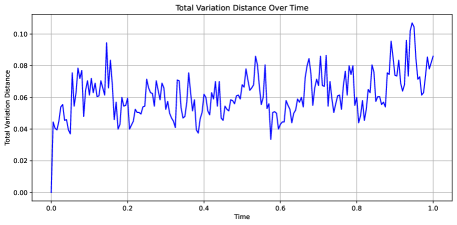
Refer to caption
Figure 2: [Example 4.1] The TV distance between PMCsuperscript𝑃MCP^{\mathrm{MC}} and PSsuperscript𝑃SP^{\mathrm{S}} for (32).

Example 4.2 (Jump-diffusion with α𝛼\alpha-stable Lévy noise).

In this example, we consider the following one-dimensional SDE:

(33) dXt=κ(ηXt)dt+σdBt+dLtα,dsubscript𝑋𝑡𝜅𝜂subscript𝑋limit-from𝑡d𝑡𝜎dsubscript𝐵𝑡dsubscriptsuperscript𝐿𝛼𝑡\displaystyle\,\mathrm{d}X_{t}=\kappa(\eta-X_{t-})\,\mathrm{d}t+\sigma\,\mathrm{d}B_{t}+\,\mathrm{d}L^{\alpha}_{t},

which has been widely used to capture dynamics with both continuous fluctuations and heavy-tailed, discontinuous shocks, making them relevant in fields such as finance, physics [2], and generative modeling [41]. This system captures mean reversion, diffusion, and an α𝛼\alpha-stable Lévy motion Ltαsubscriptsuperscript𝐿𝛼𝑡L^{\alpha}_{t} with Lévy measure:

ν(r)=cα1|r|α+1,cα=α21απΓ(1+α2)Γ(1α2),Γ(z):=0tz1etdt.formulae-sequence𝜈𝑟subscript𝑐𝛼1superscript𝑟𝛼1formulae-sequencesubscript𝑐𝛼𝛼superscript21𝛼𝜋Γ1𝛼2Γ1𝛼2assignΓ𝑧superscriptsubscript0superscript𝑡𝑧1superscript𝑒𝑡differential-d𝑡\nu(r)=c_{\alpha}\frac{1}{|r|^{\alpha+1}},\quad c_{\alpha}=\frac{\alpha}{2^{1-\alpha}\sqrt{\pi}}\frac{\Gamma(\frac{1+\alpha}{2})}{\Gamma(1-\frac{\alpha}{2})},\quad\Gamma(z):=\int_{0}^{\infty}t^{z-1}e^{-t}\,\mathrm{d}t.
Refer to caption
Refer to caption
Figure 3: [Example 4.2] Probability flows of (33).

We set α=1.5𝛼1.5\alpha=1.5 while keeping all other hyperparameters the same as in Example 4.1. To avoid the singularity of the intensity measure ν𝜈\nu at 00, the numerical integration with respect to ν(r)𝜈𝑟\nu(r) is restricted to the interval [5,0.01][0.01,5]50.010.015[-5,-0.01]\cup[0.01,5]. In this example, the Monte Carlo simulation is based on the following Euler–Maruyama scheme: Xt+Δt(i)=Xt(i)+κ(ηXt(i))Δt+σξt+ΔLtα,i=1,,Nformulae-sequencesuperscriptsubscript𝑋𝑡Δ𝑡𝑖superscriptsubscript𝑋𝑡𝑖𝜅𝜂superscriptsubscript𝑋𝑡𝑖Δ𝑡𝜎subscript𝜉𝑡Δsubscriptsuperscript𝐿𝛼𝑡𝑖1𝑁X_{t+\Delta t}^{(i)}=X_{t}^{(i)}+\kappa(\eta-X_{t}^{(i)})\Delta t+\sigma\xi_{t}+\Delta L^{\alpha}_{t},\ i=1,\cdots,N, where the jump increments ΔLtα=Lt+ΔtαLtαΔsuperscriptsubscript𝐿𝑡𝛼superscriptsubscript𝐿𝑡Δ𝑡𝛼superscriptsubscript𝐿𝑡𝛼\Delta L_{t}^{\alpha}=L_{t+\Delta t}^{\alpha}-L_{t}^{\alpha} follow a stable distribution Sα(Δt1α,0,0)subscript𝑆𝛼Δsuperscript𝑡1𝛼00S_{\alpha}(\Delta t^{\frac{1}{\alpha}},0,0).

Figure 3 and Figure 4 depict the evolutions of probability flow and the TV distance between PMCsuperscript𝑃MCP^{\mathrm{MC}} and PSsuperscript𝑃SP^{\mathrm{S}}. The proposed method demonstrates convincing performance in handling α𝛼\alpha-stable Lévy processes and singular intensity measures, maintaining a TV distance on the order of 102superscript10210^{-2}.

Refer to caption
Figure 4: [Example 4.2] The TV distance between PMCsuperscript𝑃MCP^{\mathrm{MC}} and PSsuperscript𝑃SP^{\mathrm{S}} for (33).

Example 4.3 (Double-well system with interaction force).

Next, we consider the following two-dimensional interactive SDE:

(34) dXt=dsubscript𝑋𝑡absent\displaystyle\,\mathrm{d}X_{t}= (XtXt3)dt+Kp^t(Xt)dt+σdBt1+JtdNt,subscript𝑋limit-from𝑡superscriptsubscript𝑋limit-from𝑡3d𝑡𝐾subscript^𝑝𝑡subscript𝑋limit-from𝑡d𝑡𝜎dsubscriptsuperscript𝐵1𝑡subscript𝐽𝑡dsubscript𝑁𝑡\displaystyle\ (X_{t-}-X_{t-}^{3})\,\mathrm{d}t+K*\widehat{p}_{t}(X_{t-})\,\mathrm{d}t+\sigma\,\mathrm{d}B^{1}_{t}+J_{t}\,\mathrm{d}N_{t},
dYt=dsubscript𝑌𝑡absent\displaystyle\,\mathrm{d}Y_{t}= Ytdt+Kp^t(Yt)dt+σdBt2,subscript𝑌limit-from𝑡d𝑡𝐾subscript^𝑝𝑡subscript𝑌limit-from𝑡d𝑡𝜎dsubscriptsuperscript𝐵2𝑡\displaystyle\ Y_{t-}\,\mathrm{d}t+K*\widehat{p}_{t}(Y_{t-})\,\mathrm{d}t+\sigma\,\mathrm{d}B^{2}_{t},

where the interaction kernel is K(x)=x𝐾𝑥𝑥K(x)=x. We set the parameters σ𝜎\sigma and Jtsubscript𝐽𝑡J_{t} to be the same as those in Example 4.1, and the Monte Carlo simulation is based on the following Euler–Maruyama method:

(35) Xt+Δt(i)=superscriptsubscript𝑋𝑡Δ𝑡𝑖absent\displaystyle X_{t+\Delta t}^{(i)}= Xt(i)+(Xt(i)(Xt(i))3)Δt+1Nj=1NK(Xt(i)Xt(j))Δt+σξt1+k=1NΔtJk,superscriptsubscript𝑋𝑡𝑖superscriptsubscript𝑋𝑡𝑖superscriptsuperscriptsubscript𝑋𝑡𝑖3Δ𝑡1𝑁superscriptsubscript𝑗1𝑁𝐾superscriptsubscript𝑋𝑡𝑖superscriptsubscript𝑋𝑡𝑗Δ𝑡𝜎subscriptsuperscript𝜉1𝑡superscriptsubscript𝑘1subscript𝑁Δ𝑡subscript𝐽𝑘\displaystyle\ X_{t}^{(i)}+(X_{t}^{(i)}-(X_{t}^{(i)})^{3})\Delta t+\frac{1}{N}\sum_{j=1}^{N}K(X_{t}^{(i)}-X_{t}^{(j)})\Delta t+\sigma\xi^{1}_{t}+\sum_{k=1}^{N_{\Delta t}}J_{k},
Yt+Δt(i)=superscriptsubscript𝑌𝑡Δ𝑡𝑖absent\displaystyle Y_{t+\Delta t}^{(i)}= Yt(i)+Yt(i)Δt+1Nj=1NK(Yt(i)Yt(j))Δt+σξt2,i=1,,N,formulae-sequencesuperscriptsubscript𝑌𝑡𝑖superscriptsubscript𝑌𝑡𝑖Δ𝑡1𝑁superscriptsubscript𝑗1𝑁𝐾superscriptsubscript𝑌𝑡𝑖superscriptsubscript𝑌𝑡𝑗Δ𝑡𝜎subscriptsuperscript𝜉2𝑡𝑖1𝑁\displaystyle\ Y_{t}^{(i)}+Y_{t}^{(i)}\Delta t+\frac{1}{N}\sum_{j=1}^{N}K(Y_{t}^{(i)}-Y_{t}^{(j)})\Delta t+\sigma\xi^{2}_{t},\quad i=1,\cdots,N,

where ξt1subscriptsuperscript𝜉1𝑡\xi^{1}_{t} and ξt2subscriptsuperscript𝜉2𝑡\xi^{2}_{t} are independent random variables sampled from the Gaussian distribution N0,ΔtsubscriptN0Δ𝑡\mathrm{N}_{0,\Delta t}.

Refer to caption
Refer to caption
Refer to caption
Refer to caption
Figure 5: [Example 4.3] The Probability flows of (34) along the axes: x𝑥x (top), and y𝑦y (bottom).
Refer to caption
Refer to caption
Refer to caption
Refer to caption
Figure 6: [Example 4.3] Kernel density estimation (KDE) of distributions for 400040004000 samples in the xy𝑥𝑦xy-plane. Top: Monte Carlo simulation (35); Bottom: results from Algorithm 1. From left to right: the distributions are shown at the 00th, 404040th, 100100100th, and 250250250th time steps.

Figure 5 illustrates the evolution of probability flows obtained from Equation (34), computed using both the Monte Carlo simulation and the proposed approach. Figure 6 depicts the probability flow evolution on the xy𝑥𝑦xy-plane at different time steps for both methods. Finally, Figure 7 presents the TV distance between PMCsuperscript𝑃MCP^{\mathrm{MC}} and PSsuperscript𝑃SP^{\mathrm{S}}, consistently demonstrating values on the order of 102superscript10210^{-2}. These results confirm the accuracy of the proposed method in approximating the probability flows for systems with interaction terms.
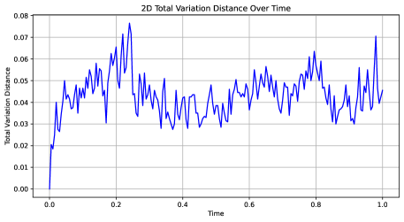
Refer to caption
Figure 7: [Example 4.3] The TV distance between PMCsuperscript𝑃MCP^{\mathrm{MC}} and PSsuperscript𝑃SP^{\mathrm{S}} for (34).

Example 4.4 (State-dependent jump-diffusion).

To conclude our numerical study, we consider the following three-dimensional SDE which describes the asset price dynamics under both jump and stochastic volatility conditions[23]

(36) dst=dsubscript𝑠𝑡absent\displaystyle\,\mathrm{d}s_{t}= (γδvt/2Λ(vt,mt)J¯)dt+|vt|dBt1+log(Jts+1)dNt,𝛾𝛿subscript𝑣limit-from𝑡2Λsubscript𝑣limit-from𝑡subscript𝑚limit-from𝑡¯𝐽d𝑡subscript𝑣limit-from𝑡dsuperscriptsubscript𝐵𝑡1subscriptsuperscript𝐽𝑠𝑡1dsubscript𝑁𝑡\displaystyle\ (\gamma-\delta-v_{t-}/2-\Lambda(v_{t-},m_{t-})\bar{J})\,\mathrm{d}t+\sqrt{|v_{t-}|}\,\mathrm{d}B_{t}^{1}+\log(J^{s}_{t}+1)\,\mathrm{d}N_{t},
dvt=dsubscript𝑣𝑡absent\displaystyle\,\mathrm{d}v_{t}= κv(mtvt)dt+σv|vt|(dBt1+1ρ2dBt2)+JtvdNt,subscript𝜅𝑣subscript𝑚limit-from𝑡subscript𝑣limit-from𝑡d𝑡subscript𝜎𝑣subscript𝑣limit-from𝑡dsubscriptsuperscript𝐵1𝑡1superscript𝜌2dsuperscriptsubscript𝐵𝑡2subscriptsuperscript𝐽𝑣𝑡dsubscript𝑁𝑡\displaystyle\ \kappa_{v}(m_{t-}-v_{t-})\,\mathrm{d}t+\sigma_{v}\sqrt{|v_{t-}|}(\,\mathrm{d}B^{1}_{t}+\sqrt{1-\rho^{2}}\,\mathrm{d}B_{t}^{2})+J^{v}_{t}\,\mathrm{d}N_{t},
dmt=dsubscript𝑚𝑡absent\displaystyle\,\mathrm{d}m_{t}= κm(αmmt)dt+σm|mt|dBt3.subscript𝜅𝑚subscript𝛼𝑚subscript𝑚limit-from𝑡d𝑡subscript𝜎𝑚subscript𝑚limit-from𝑡dsubscriptsuperscript𝐵3𝑡\displaystyle\ \kappa_{m}(\alpha_{m}-m_{t-})\,\mathrm{d}t+\sigma_{m}\sqrt{|m_{t-}|}\,\mathrm{d}B^{3}_{t}.

Here Bt=(Bt1,Bt2,Bt3)subscript𝐵𝑡superscriptsubscript𝐵𝑡1superscriptsubscript𝐵𝑡2superscriptsubscript𝐵𝑡3B_{t}=(B_{t}^{1},B_{t}^{2},B_{t}^{3}) is the standard Brownian motion in 3superscript3\mathbb{R}^{3} and Ntsubscript𝑁𝑡N_{t} is an independent Poisson process with the state-dependent rate Λ(v,m)=Λ0+Λ1v+Λ2mΛ𝑣𝑚subscriptΛ0subscriptΛ1𝑣subscriptΛ2𝑚\Lambda(v,m)=\Lambda_{0}+\Lambda_{1}v+\Lambda_{2}m. The jump component Jtvsuperscriptsubscript𝐽𝑡𝑣J_{t}^{v} follows the exponential distribution with the expectation μJvsubscriptsuperscript𝜇𝑣𝐽\mu^{v}_{J}. Meanwhile, the jump component for the stock price, Jtssuperscriptsubscript𝐽𝑡𝑠J_{t}^{s}, follows a shifted log-normal distribution, where Jts+1superscriptsubscript𝐽𝑡𝑠1J_{t}^{s}+1 is characterized by the parameters μssubscript𝜇𝑠\mu_{s} and σssubscript𝜎𝑠\sigma_{s}, leading to 𝔼(Jts)=J¯=exp(μs+σs2/2)1𝔼subscriptsuperscript𝐽𝑠𝑡¯𝐽subscript𝜇𝑠superscriptsubscript𝜎𝑠221\mathbb{E}(J^{s}_{t})=\bar{J}=\exp(\mu_{s}+\sigma_{s}^{2}/2)-1.The parameters are from [23] and specified as follows: (γ,δ,κv,κm,αm,σv,σm,ρ)𝛾𝛿subscript𝜅𝑣subscript𝜅𝑚subscript𝛼𝑚subscript𝜎𝑣subscript𝜎𝑚𝜌(\gamma,\delta,\kappa_{v},\kappa_{m},\alpha_{m},\sigma_{v},\sigma_{m},\rho) = (0.04,0.015,3.1206,3.3168,0.1125,0.394,0.0835,0.688)0.040.0153.12063.31680.11250.3940.08350.688(0.04,0.015,3.1206,3.3168,0.1125,0.394,0.0835,-0.688), (Λ0,Λ1,Λ2)=(2.096,21.225,0)subscriptΛ0subscriptΛ1subscriptΛ22.09621.2250(\Lambda_{0},\Lambda_{1},\Lambda_{2})=(2.096,21.225,0), and (μs,σs,μJv)=(0.012,0.043,0.002)subscript𝜇𝑠subscript𝜎𝑠superscriptsubscript𝜇𝐽𝑣0.0120.0430.002(\mu_{s},\sigma_{s},\mu_{J}^{v})=(-0.012,0.043,0.002).

We set the initial condition as a three-dimensional Gaussian distribution with the mean vector (5,5,5)superscript555top(5,5,5)^{\top} and the covariance matrix of a 3×3333\times 3 identity matrix. The numerical integration for r𝑟r is performed over a two-dimensional uniform grid defined on [0.17,0.17]×[0,0.0015]0.170.1700.0015[-0.17,0.17]\times[0,0.0015], which is designed to capture the critical density features required for accurate numerical evaluation. The Monte Carlo approximation is easy to achieve by noting that the numerical approximation of log(Jts+1)dNtsubscriptsuperscript𝐽𝑠𝑡1dsubscript𝑁𝑡\log(J^{s}_{t}+1)\,\mathrm{d}N_{t} is k=1NΔtξkJssuperscriptsubscript𝑘1subscript𝑁Δ𝑡subscriptsuperscript𝜉superscript𝐽𝑠𝑘\sum_{k=1}^{N_{\Delta t}}\xi^{J^{s}}_{k} where {ξkJs}ksubscriptsubscriptsuperscript𝜉superscript𝐽𝑠𝑘𝑘\{\xi^{J^{s}}_{k}\}_{k\in\mathbb{N}} are i.i.d samples from the law of log(Jts+1)superscriptsubscript𝐽𝑡𝑠1\log(J_{t}^{s}+1) and NΔtPo(ΛΔt)similar-tosubscript𝑁Δ𝑡PoΛΔ𝑡N_{\Delta t}\sim\text{Po}(\Lambda\Delta t). Similarly JtvdNtsuperscriptsubscript𝐽𝑡𝑣dsubscript𝑁𝑡J_{t}^{v}\,\mathrm{d}N_{t} is approximated by k=1NΔtξkJvsuperscriptsubscript𝑘1subscript𝑁Δ𝑡subscriptsuperscript𝜉superscript𝐽𝑣𝑘\sum_{k=1}^{N_{\Delta t}}\xi^{J^{v}}_{k} where {ξkJv}ksubscriptsubscriptsuperscript𝜉superscript𝐽𝑣𝑘𝑘\{\xi^{J^{v}}_{k}\}_{k\in\mathbb{N}} are i.i.d samples from the law of Jvssuperscriptsubscript𝐽𝑣𝑠J_{v}^{s}.

Let Xt=(st,vt,mt)subscript𝑋𝑡superscriptsubscript𝑠𝑡subscript𝑣𝑡subscript𝑚𝑡topX_{t}=(s_{t},v_{t},m_{t})^{\top}, the SDE (36) can be rewritten as

dXt=dsubscript𝑋𝑡absent\displaystyle\,\mathrm{d}X_{t}= [(γδλ0J¯0κmαm)+(01/2Λ1J¯Λ2J¯0κvκv00κm)Xt]dtdelimited-[]matrix𝛾𝛿subscript𝜆0¯𝐽0subscript𝜅𝑚subscript𝛼𝑚matrix012subscriptΛ1¯𝐽subscriptΛ2¯𝐽0subscript𝜅𝑣subscript𝜅𝑣00subscript𝜅𝑚subscript𝑋𝑡d𝑡\displaystyle\ \left[\left(\begin{matrix}\gamma-\delta-\lambda_{0}\bar{J}\\ 0\\ \kappa_{m}\alpha_{m}\\ \end{matrix}\right)+\left(\begin{matrix}0&-1/2-\Lambda_{1}\bar{J}&-\Lambda_{2}\bar{J}\\ 0&-\kappa_{v}&\kappa_{v}\\ 0&0&-\kappa_{m}\end{matrix}\right)X_{t}\right]\,\mathrm{d}t
+(|vt|00σv|vt|σv|vt|1ρ2000σm|mt|)dBt+3(log(r1+1)r20)𝒩(dt,dr),matrixsubscript𝑣𝑡00subscript𝜎𝑣subscript𝑣𝑡subscript𝜎𝑣subscript𝑣𝑡1superscript𝜌2000subscript𝜎𝑚subscript𝑚𝑡dsubscript𝐵𝑡subscriptsuperscript3matrixsubscript𝑟11subscript𝑟20𝒩d𝑡d𝑟\displaystyle\ +\left(\begin{matrix}\sqrt{|v_{t}|}&0&0\\ \sigma_{v}\sqrt{|v_{t}|}&\sigma_{v}\sqrt{|v_{t}|}\sqrt{1-\rho^{2}}&0\\ 0&0&\sigma_{m}\sqrt{|m_{t}|}\end{matrix}\right)\,\mathrm{d}B_{t}+\int_{\mathbb{R}^{3}}\left(\begin{matrix}\log(r_{1}+1)\\ r_{2}\\ 0\end{matrix}\right)\mathcal{N}(\,\mathrm{d}t,\,\mathrm{d}r),

where 𝒩𝒩\mathcal{N} denotes a random Poisson measure on +×3subscriptsuperscript3\mathbb{R}_{+}\times\mathbb{R}^{3} with Lévy measure dt×Λ(vt,mt)νJ(dr)d𝑡Λsubscript𝑣𝑡subscript𝑚𝑡subscript𝜈𝐽d𝑟\,\mathrm{d}t\times\Lambda(v_{t},m_{t})\nu_{J}(\,\mathrm{d}r), and the jump-size measure νJ(dr)=νJs(dr1)×νJv(dr2)×νJm(dr3)subscript𝜈𝐽d𝑟subscript𝜈superscript𝐽𝑠dsubscript𝑟1subscript𝜈superscript𝐽𝑣dsubscript𝑟2subscript𝜈superscript𝐽𝑚dsubscript𝑟3\nu_{J}(\,\mathrm{d}r)=\nu_{J^{s}}(\,\mathrm{d}r_{1})\times\nu_{J^{v}}(\,\mathrm{d}r_{2})\times\nu_{J^{m}}(\,\mathrm{d}r_{3}). In this expression, F(r,t)=G(r,t)=(log(r1+1),r2,0)𝐹𝑟𝑡𝐺𝑟𝑡superscriptsubscript𝑟11subscript𝑟20topF(r,t)=G(r,t)=(\log(r_{1}+1),r_{2},0)^{\top} .

Refer to caption
Refer to caption
Refer to caption
Refer to caption
Refer to caption
Refer to caption
Figure 8: [Example 4.4] Probability flows along the axes: s𝑠s (top), v𝑣v (middle), and m𝑚m (bottom).

Figure 8 illustrates the evolution of probability flows for each marginal derived from Equation (36). Figure 9 presents the TV distance between the probabilities PMCsuperscript𝑃MCP^{\mathrm{MC}} and PSsuperscript𝑃SP^{\mathrm{S}}, demonstrating that the distance remains on the order of 102superscript10210^{-2}. These results highlight the capability of our proposed method to accurately and efficiently solve complex state-dependent jump-diffusion systems.
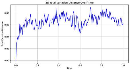
Refer to caption
Figure 9: [Example 4.4] The TV distance between PMCsuperscript𝑃MCP^{\mathrm{MC}} and PSsuperscript𝑃SP^{\mathrm{S}} for (36).

5 Conclusions

In this paper, we introduced the concept of the generalized score function, which unifies the conventional diffusion score and the Lévy score, thereby accommodating a broad class of non-Gaussian processes. Leveraging this generalized score function, we developed a score-based particle algorithm to efficiently solve the nonlinear Lévy-Fokker-Planck equation through sampling of probability flow data. Furthermore, we demonstrate that the Kullback-Leibler divergence between the numerical solution and the ground truth is bounded by a specific loss function, derived from a fixed-point perspective. The rigorous numerical analysis was conducted to validate the theoretical properties of our algorithm. Finally, several numerical examples were presented to illustrate the effectiveness and accuracy of the proposed method.

Data Availability

The datasets generated and/or analyzed during the current study are available in the GitHub reposItôry, accessible via the following link: https://github.com/cliu687/sbtm-levy. All scripts and supporting files necessary to reproduce the findings are openly provided in this reposItôry.

References

  • [1] D. Applebaum, Lévy processes and stochastic calculus, Cambridge university press, 2009.
  • [2] T. Ariga, K. Tateishi, M. Tomishige, and D. Mizuno, Noise-induced acceleration of single molecule kinesin-1, Physical review letters, 127 (2021), p. 178101.
  • [3] P. Barthelemy, J. Bertolotti, and D. S. Wiersma, A Lévy flight for light, Nature, 453 (2008), pp. 495–498.
  • [4] N. M. Boffi and E. Vanden-Eijnden, Probability flow solution of the Fokker–Planck equation, Machine Learning: Science and Technology, 4 (2023), p. 035012.
  • [5] N. M. Boffi and E. Vanden-Eijnden, Deep learning probability flows and entropy production rates in active matter, P NATL ACAD SCI USA, 121 (2024), p. e2318106121.
  • [6] L. Caffarelli and L. Silvestre, An extension problem related to the fractional Laplacian, Communications in partial differential equations, 32 (2007), pp. 1245–1260.
  • [7] Y. Cao, J. Chen, Y. Luo, and X. Zhou, Exploring the optimal choice for generative processes in diffusion models: Ordinary vs stochastic differential equations, Advances in Neural Information Processing Systems, 36 (2024).
  • [8] H. Chen, H. Lee, and J. Lu, Improved analysis of score-based generative modeling: User-friendly bounds under minimal smoothness assumptions, in Proceedings of the 40th International Conference on Machine Learning, vol. 202, 2023, pp. 4735–4763.
  • [9] J. Chevallier and S. Goutte, Estimation of Lévy-driven Ornstein–Uhlenbeck processes: Application to modeling of CO2 and fuel-switching, Annals of Operations Research, 255 (2017), pp. 169–197.
  • [10] V. De Bortoli, J. Thornton, J. Heng, and A. Doucet, Diffusion Schrödinger bridge with applications to score-based generative modeling, in Advances in Neural Information Processing Systems, vol. 34, Curran Associates, Inc., 2021, pp. 17695–17709.
  • [11] P.-E. C. de Raynal, J.-F. Jabir, and S. Menozzi, Multidimensional stable driven Mckean–Vlasov SDEs with distributional interaction kernel: a regularization by noise perspective, Stochastics and Partial Differential Equations: Analysis and Computations, (2024), pp. 1–54.
  • [12] D. Gallon, A. Jentzen, and P. von Wurstemberger, An overview of diffusion models for generative artificial intelligence, arXiv preprint arXiv:2412.01371, (2024).
  • [13] F. Golse, On the dynamics of large particle systems in the mean field limit, Macroscopic and large scale phenomena: coarse graining, mean field limits and ergodicity, (2016), pp. 1–144.
  • [14] G. Gottwald, F. Li, Y. Marzouk, and S. Reich, Stable generative modeling using diffusion maps, arXiv preprint arXiv:2401.04372, (2024).
  • [15] J. Ho, A. Jain, and P. Abbeel, Denoising diffusion probabilistic models, in Advances in Neural Information Processing Systems, vol. 33, Curran Associates, Inc., 2020, pp. 6840–6851.
  • [16] Z. Hu, Z. Zhang, G. E. Karniadakis, and K. Kawaguchi, Score-fPINN: Fractional score-based physics-informed neural networks for high-dimensional Fokker-Planck-Lévy equations, arXiv preprint arXiv:2406.11676, (2024).
  • [17] Y. Huang and L. Wang, A score-based particle method for homogeneous Landau equation, arXiv preprint arXiv:2405.05187, (2024).
  • [18] Y. Huang, X. Zhou, and J. Duan, Probability flow approach to the Onsager–Machlup functional for jump-diffusion processes, SIAM Applied Math(accepted). arXiv:2409.01340.
  • [19] A. Hyvärinen and P. Dayan, Estimation of non-normalized statistical models by score matching., Journal of Machine Learning Research, 6 (2005).
  • [20] V. Ilin, J. Hu, and Z. Wang, Transport based particle methods for the Fokker-Planck-Landau equation, ArXiv, abs/2405.10392 (2024).
  • [21] P.-E. Jabin and Z. Wang, Quantitative estimates of propagation of chaos for stochastic systems with W1,superscript𝑊1{W^{-1,\infty}} kernels, Inventiones mathematicae, 214 (2018), pp. 523–591.
  • [22] K. Kanazawa, T. G. Sano, A. Cairoli, and A. Baule, Loopy Lévy flights enhance tracer diffusion in active suspensions, Nature, 579 (2020), pp. 364–367.
  • [23] D. Kristensen, Y. J. Lee, and A. Mele, Closed-form approximations of moments and densities of continuous–time Markov models, Journal of Economic Dynamics and Control, (2024), p. 104948.
  • [24] L. Li, S. Hurault, and J. Solomon, Self-consistent velocity matching of probability flows, in Thirty-seventh Conference on Neural Information Processing Systems, 2023.
  • [25] M. Liang, M. B. Majka, and J. Wang, Exponential ergodicity for SDEs and Mckean–Vlasov processes with Lévy noise, Annales de l’Institut Henri Poincare (B) Probabilites et statistiques, 57 (2021), pp. 1665–1701.
  • [26] H. Liu and J. Y. Lin, Stochastic Mckean–Vlasov equations with Lévy noise: Existence, attractiveness and stability, Chaos, Solitons & Fractals, 177 (2023), p. 114214.
  • [27] Y. Liu, M. Yang, Z. Zhang, F. Bao, Y. Cao, and G. Zhang, Diffusion-model-assisted supervised learning of generative models for density estimation, Journal of Machine Learning for Modeling and Computing, 5 (2024).
  • [28] J. Lu, Y. Wu, and Y. Xiang, Score-based transport modeling for mean-field Fokker-Planck equations, Journal of Computational Physics, 503 (2024), p. 112859.
  • [29] D. Maoutsa, S. Reich, and M. Opper, Interacting particle solutions of Fokker–Planck equations through gradient–log–density estimation, Entropy, 22 (2020), p. 802.
  • [30] C. Olivera and M. Simon, Microscopic derivation of non-local models with anomalous diffusions from stochastic particle systems, arXiv preprint arXiv:2404.03772, (2024).
  • [31] F. Santambrogio, Optimal transport for applied mathematicians, Birkäuser, NY, 55 (2015).
  • [32] Z. Shen and Z. Wang, Entropy-dissipation informed neural network for Mckean-Vlasov type PDEs, Advances in Neural Information Processing Systems, 36 (2024).
  • [33] Z. Shen, Z. Wang, S. Kale, A. Ribeiro, A. Karbasi, and H. Hassani, Self-consistency of the Fokker–Planck equation, in Conference on Learning Theory, PMLR, 2022, pp. 817–841.
  • [34] J. Song, C. Meng, and S. Ermon, Denoising diffusion implicit models, in International Conference on Learning Representations, 2021.
  • [35] M. S. Song, H. C. Moon, J.-H. Jeon, and H. Y. Park, Neuronal messenger ribonucleoprotein transport follows an aging Lévy walk, Nature communications, 9 (2018), pp. 1–8.
  • [36] Y. Song and S. Ermon, Generative modeling by estimating gradients of the data distribution, in NeurIPS, vol. 32, Curran Associates, Inc., 2019.
  • [37] Y. Song, S. Garg, J. Shi, and S. Ermon, Sliced score matching: A scalable approach to density and score estimation, in Uncertainty in Artificial Intelligence, PMLR, 2020, pp. 574–584.
  • [38] Y. Song, J. Sohl-Dickstein, D. P. Kingma, A. Kumar, S. Ermon, and B. Poole, Score-based generative modeling through stochastic differential equations, International Conference on Learning Representations (ICLR), (2021).
  • [39] T. Tomé and M. Oliveira, Stochastic Dynamics and Irreversibility, Graduate Texts in Physics, Springer International Publishing, 2014.
  • [40] C. Villani et al., Optimal transport: old and new, vol. 338, Springer, 2009.
  • [41] E. B. Yoon, K. Park, S. Kim, and S. Lim, Score-based generative models with Lévy processes, Advances in Neural Information Processing Systems, 36 (2023), pp. 40694–40707.