Dynamical phase transitions in certain non-ergodic stochastic processes

Abstract

We present a class of stochastic processes in which the large deviation functions of time-integrated observables exhibit singularities that relate to dynamical phase transitions of trajectories. These illustrative examples include Brownian motion with a death rate or in the presence of an absorbing wall, for which we consider a set of empirical observables such as the net displacement, local time, residence time, and area under the trajectory. Using a backward Fokker-Planck approach, we derive the large deviation functions of these observables, and demonstrate how singularities emerge from a competition between survival and diffusion. Furthermore, we analyse this scenario using an alternative approach with tilted operators, showing that at the singular point, the effective dynamics undergoes an abrupt transition. Extending this approach, we show that similar transitions may generically arise in Markov chains with transient states. This scenario is robust and generalizable for non-Markovian dynamics and for many-body systems, potentially leading to multiple dynamical phase transitions.

I Introduction

Dynamical phase transitions (DPTs) are singular changes in the distribution of dynamical observables, manifesting as singularities in their large deviation functions. These transitions are observed in systems with many degrees of freedom, such as driven diffusive systems [1, 2, 3, 4, 5, 6, 7], lattice gas models [8, 9, 10], kinetically constrained models of glasses [11, 12], interface models [13, 14], active matter [15, 16], random graphs [17], and others [18, 19, 20, 21, 22, 23, 24]. In systems with a few degrees of freedom, DPTs were observed in the weak-noise limit of Langevin dynamics [1, 25, 26]. In recent years, there have been reports of simple models having DPTs without requiring macroscopic or low noise limits, such as in the context of reset processes [27, 28, 29, 30, 31, 32, 33, 34, 35, 36], run-and-tumble dynamics [37, 38, 39, 40, 41, 42, 43, 44], constrained Brownian motion[45, 46], drifted Brownian motion [47, 48, 49], driven random walker [40, 50, 51], vicious Brownian walkers [52], active Brownian particles [53], Brownian motion with dry friction [54], Brownian motion with certain special observables [55, 56] or in higher dimensions [56].

In this paper, we argue that DPTs could generically arise in certain non-ergodic stochastic processes without the need for weak-noise or macroscopic limit. This scenario provides a unifying narrative for the DPTs reported earlier in several seemingly unrelated models [27, 28, 34, 40, 48, 47, 50, 54, 52, 44]. Understanding the mechanism helps us construct interesting phase behaviours for many-body systems and their extensions in non-Markovian processes.

We present the scenario for illustrative examples of one-dimensional Brownian motion, $X_{t}$, in which non-ergodicity is introduced by a leaking probability in the dynamics, caused, for example, by an absorption site. We consider several different empirical observables for the process $X_{t}$, which are of the form [57, 58, 59, 60, 61]

$$Q=\int_{0}^{T}dt\;U(X_{t})+\int_{0}^{T}dX_{t}\;V(X_{t}),$$ (1)

where $U$ and $V$ are functions of $X_{t}$. The second integral in (1) is interpreted as a stochastic integral with a Stratonovich discretisation.

The dynamical observable $Q$ is a functional of the Brownian trajectory and a fluctuating quantity that depends on a particular realization of the process. The probability of $Q$ can be systematically analyzed using a well-established framework for Brownian functionals [62]. In our explicit examples, we consider four different observables for the Brownian motion: (a) net displacement ($U=0$, $V=1$), (b) local time at position $a$ ($U(x)=\delta(x-a)$, $V=0$), (c) residence time in an interval ($U(x)=1$ for $a<x<b$ and zero outside, $V=0$), and (d) area under the Brownian trajectory ($U=x$ and $V(x)=0$).

We explore these observables for two specific Brownian dynamics. In the first example, a mortal Brownian particle has a probability of dying rendering it immobile. In the second example, the Brownian motion is constrained to move between a fixed absorbing wall and a reflecting wall. For both examples, we show that the probability $P_{T}(Q)$ of $Q$ typically (with exceptions discussed in the text) takes a large deviation form for large $T$,

$$P_{T}(Q=qT)\sim e^{-T\phi(q)},$$ (2)

where $\phi(q)$ is the large deviations function (ldf). For the four observables defined above, we determine $\phi(q)$ using the framework in [62] and show that for all four observables, $\phi(q)$ is singular at certain values of $q$.

These singularities are linked to the dynamical phase transitions, arising from the interplay between trajectories that persist without being dead or absorbed throughout the entire duration $T$ and trajectories that do not survive. Depending on the value of $Q$, one of these two kinds of trajectories is optimal for large $T$, and the singular point in $\phi(q)$ marks the transition between these two types of evolutions. This represents a path-space generalization of conventional equilibrium phase transitions, where singularity in thermodynamic free energy indicates transitions in static observables.

An insightful approach to quantify the differences in the nature of trajectories is in terms of an effective dynamics [59, 63, 58, 61, 64, 65, 66]. Employing a theory of constrained dynamics [57, 59, 60, 61], we show that in our examples, the effective dynamics attaining a value of $Q$ for large $T$ is described by a Langevin process, whose nature changes across the DPT.

The theory of constrained dynamics [57, 58, 59, 60, 61] draws parallels between the mechanism of DPTs and equilibrium phase transitions. In equilibrium lattice models, the singularity of the free energy at a phase transition is associated with the crossing of leading eigenvalues of a transfer matrix [67, 68, 69]. The singularity of $\phi(q)$ in DPTs is related to a similar crossing of two largest eigenvalues of a tilted operator. Typically, such a crossing of eigenvalues is forbidden by the Perron-Frobenius-Jentz theorem [69], unless the tilted operator falls outside the domain of the theorem. This indeed occurs for reducible tilted operators in non-ergodic stochastic processes like those in our examples. This offers a unifying perspective on the origin of DPTs in non-ergodic stochastic processes.

We illustrate the generality of this mechanism in Markov chains with transient state spaces where eigenvalue crossing results in DPTs of observables that are discrete analogs of (1). The mechanism extends to many-body systems and non-Markovian processes. Our work asserts earlier observations [47, 48, 40, 52, 50, 54, 51] of DPTs in non-ergodic dynamics.

The paper is organized in the following order. After a brief introduction about relevant concepts of large deviations in Sec II, we discuss DPTs for mortal Brownian motion in Sec III and for Brownian motion in presence of an absorbing boundary in Sec IV. These results obtained using the backward Fokker-Planck approach [62] are then reproduced using an alternative approach of tilted operators in Sec V. An extension of the DPTs for Markov chains is discussed in Sec VI with a general scenario presented in Sec VII. In Sec VIII, we present examples of many-particle systems with a sequence of DPTs. Examples of DPTs in non-Markov processes is discussed in Sec IX, with applications in fractional Brownian motion and in a model of active matter. We conclude in Sec X with a discussion about open directions.

II Large deviation theory

The large deviation asymptotic in (2) precisely means

$$\lim_{T\to\infty}\frac{1}{T}\ln P_{T}(Q=qT)=-\phi(q).$$ (3)

This is equivalent to an asymptotic of the generating function

$$\langle e^{pQ}\rangle\sim e^{T\mu(p)}$$ (4)

for large $T$, where $\mu(p)$ is the scaled cumulant generating function (scgf). The scgf relates to the large deviation function $\phi(q)$ by a Legendre-Fenchel transformation

$$\mu(p)=\max_{q}\{pq-\phi(q)\}.$$ (5)

For an introduction to the large deviation theory see [70, 71].

III Mortal Brownian motion

The simplest continuous model we consider is the motion of a one-dimensional Brownian particle with a probability rate $\alpha$ of dying, after which the particle remains immobile forever. In a small time interval $dt$, the position $x_{t}$ of an alive particle evolves via the Langevin equation

$$x_{t+dt}=\begin{dcases}x_{t}&\textrm{with prob }\alpha dt\ \textrm{of death}\\ x_{t}+\eta_{t}dt&\textrm{with prob}\ 1-\alpha dt,\end{dcases}$$ (6)

where $\eta_{t}$ is a Gaussian white noise with zero mean and the correlator $\langle\eta_{t}\eta_{t^{\prime}}\rangle=2D\delta(t-t^{\prime})$. For simplicity, we henceforth set $D=1$ for the rest of the paper. In the above equation, once the particle dies, $x_{t+dt}=x_{t}$ for the rest of time. Similar diffusion processes with mortality have been studied in related contexts [72, 73, 74, 75, 76].

The dynamics can also be described by the Fokker-Planck equation for the probability $$P_{t}^{(a)}(x) t x$$ for the particle to start at the origin and remain alive until time , at which point it is at position ,

$$\partial_{t}P^{(a)}_{t}(x)=\partial_{x}^{2}P^{(a)}_{t}(x)-\alpha P^{(a)}_{t}(x)$$ (7a)

with the initial condition $$P_{0}^{(a)}(x)=\delta(x) x t$$. The probability for the particle to be dead at position at time follows

$$\partial_{t}P^{(d)}_{t}(x)=\alpha P^{(a)}_{t}(x)$$ (7b)

with the initial condition $P_{0}^{(d)}(x)=0$. The probability of a particle to be at $x$, irrespective of its status (alive or dead), corresponds to the combined probabilities of two types of trajectories: those that persist until the final time $t$ and are located at $x$, and those that die at $x$ before the final time,

$$P_{t}(x)=P^{(a)}_{t}(x)+P^{(d)}_{t}(x).$$ (8)

A straightforward solution of (7b) gives

$$P_{t}(x)=e^{-\alpha t}g_{t}(x)+\alpha\int_{0}^{t}d{t^{\prime}}\,e^{-\alpha t^{\prime}}g_{t^{\prime}}(x)$$ (9)

where $g_{t}(x)=(4\pi t)^{-\frac{1}{2}}\exp(-x^{2}/4t)$ is the probability for a free Brownian starting at the origin to reach $x$ at time $t$. The first term in the solution is due to particles that remain alive throughout the entire duration, where $e^{-\alpha t}$ is the corresponding surviving probability. The second term is the net contribution from particles that survive until any intermediate time $t^{\prime}<t$ reaching location $x$ and die in the interval between $t^{\prime}$ and $t^{\prime}+dt^{\prime}$.

For large time $t=T$ with $x=qT$, the first term on the right hand side of (9) has an asymptotic $e^{-T(\alpha+q^{2}/4)}$, while the second term decays as $e^{-T\phi(q)}$ with

$$\phi(q)=\begin{dcases}|q|\sqrt{\alpha}&0\leq|q|<\sqrt{4\alpha}\\ \alpha+\frac{q^{2}}{4}&|q|\geq\sqrt{4\alpha}.\end{dcases}$$ (10)

The latter asymptotic is obtained by introducing a change of variable $t^{\prime}=rT$ and subsequently evaluating the integral in (9) using a saddle point approximation for large $T$. The non-analyticity in (10) arises because, for $|q|>\sqrt{4\alpha}$, the saddle-point value of $r=r^{\star}\equiv|q|/\sqrt{4\alpha}$ falls outside the range of integration. As a result, the integration is dominated by the value of the integrand at $r=1$ where it is maximum.

For large $T$, the asymptotic of $P_{T}(x)$ is determined by the dominant contribution among the two terms in (9) leading to (2) for $Q\equiv x$ with the ldf $\phi(q)$ in (10).

The ldf is plotted in Fig. 1 revealing singularities at $q=\pm\sqrt{4\alpha}$, where $\phi^{\prime\prime}(q)$ is discontinuous. Additionally, there is an extra singularity at $q=0$, where the first derivative $\phi^{\prime}(q)$ has a jump discontinuity. Drawing an analogy with equilibrium phase transitions, we categorise the former type of singularities as second-order DPTs and the latter type as first-order DPTs.

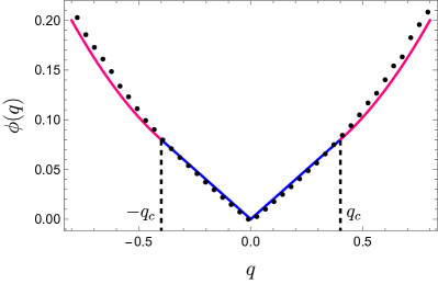
Figure 1: (color online) The solid line denotes the ldf in (10) for the distribution of position of a mortal Brownian particle with a death rate $\alpha=0.04$. The change of color at $q=\pm q_{c}$ with $q_{c}=\sqrt{4\alpha}$ highlights the second-derivative-discontinuity of $\phi(q)$ in (10). The dots on the plot represent results obtained by a Monte-Carlo simulation for $T=30$, $dt=0.01$ averaged over $10^{8}$ iterations.

The origin of the second-order transition becomes apparent through the saddle point approximation used in deriving (10). In this approximation, discussed immediately after (10), the re-scaled variable $r$ denotes the fraction of time the particle remains alive. For $|q|<\sqrt{4\alpha}$, the dominant contribution comes from the trajectories that reach $x$ and die at time $T\sqrt{4\alpha}$. In contrast, for $|q|\geq\sqrt{4\alpha}$, the dominant contribution arises from trajectories that remain alive until the final time $T$. This drastic shift in the nature of optimal trajectories gives rise to the second-order dynamical phase transition.

The first-order transition at $q=0$ stems from a similar change in the nature of optimal trajectories. For small $q$, the optimal trajectory is a straight line from the origin to $x=qT$, reaching in time $Tr^{\star}=T|q|/\sqrt{4\alpha}$ and then dying. The slope of the straight line $x/(Tr^{\star})=\textrm{sgn}(q)\sqrt{4\alpha}$ is non-vanishing for $q\to 0$, but it changes discontinuously as $q$ changes sign, leading to a first-order transition.

Remark: The ldf expression in (10) reveals that for $|q|<\sqrt{4\alpha}$, the asymptotic probability $P_{T}(x=qT)$ in (2) is time independent. This implies, for distances $|x|<T\sqrt{4\alpha}$, the distribution of position reaches a stationary state.

Remark: The same ldf in (10) was reported in the distribution of position $P_{T}(x)$ of a resetting Brownian motion [27]. This is not surprising, considering that the trajectories for $P_{T}(x)$ in the resetting Brownian motion after the last reset are related to the corresponding living part of the trajectories for the mortal Brownian motion by a reversal of time. This relation extends to other variants of the two dynamics, such as their respective generalisations for non-Markovian processes like fractional Brownian motion (see Section. IX.2).

Remark: The solution in (9) follows

$$\partial_{t}P_{t}(x)=\partial_{x}^{2}P_{t}(x)-\alpha P_{t}(x)+\alpha\delta(x)$$ (11)

with the initial condition $P_{0}(x)=\delta(x)$. The same equation was observed for the resetting Brownian motion [27], where the interpretation of the terms in (11) is clear. For the mortal Brownian motion studied here, (11) can be interpreted in a slightly different way. We note that $P_{t}(x)$ is the probability density of the mortal walker to be at $x$ at time $t$. Now, we split the time interval $[0,t+dt]$ into two segments $[0,dt]$ and $[dt,t+dt]$. In the initial interval $dt$, the particle, starting at the origin, jumps to $dx$ with probability $(1-\alpha dt)$ and dies (and therefore stays at $x=0$) with the complementary probability $\alpha dt$. For the second interval $[dt,t+dt]$, the particle has to reach $x$ starting at $dx$ in time $t$, which is equal to the probability that it reaches $x-dx$ in time $t$ stating at the origin. Considering these contributions, one can write the backward evolution equation of $P_{t}(x)$ as

$$P_{t+dt}(x)=(1-\alpha dt)\langle P_{t}(x-dx)\rangle+\alpha dt\delta(x)$$ (12)

where $\langle\rangle$ denotes an average over the initial jump $dx=\eta(0)dt$, where $\eta(0)$ is the initial noise. Taylor expanding $P_{t}(x-dx)$ and using the fact that $\langle\eta(0)\rangle=0$ and $\langle\eta^{2}(0)\rangle=\frac{2}{dt}$, we recover (11) in the limit $dt\to 0$.

Remark: The noticeable deviation in Fig. 1 between numerical and theoretical results for large $q$ is due to limitations of the direct sampling method, which fails to generate the very low probability events contributing to rare fluctuations. To capture these, one needs to employ ‘importance sampling’ algorithms [77], which have been shown in a closely related problem [78] to achieve perfect agreement with the theory.

III.1 Area under the trajectory

Another interesting observable is the area covered by a trajectory [62], defined as $Q=\int_{0}^{t_{f}}X_{t}dt$, where $t_{f}$ is the time at which the particle died. Similar to (8), the probability $P_{t}(Q)$ measured at time $t$ can be written as a combination of two parts

$$P_{t}(Q)=P^{(a)}_{t}(Q)+P^{(d)}_{t}(Q)$$ (13)

where $P^{(a)}_{t}(Q)$ is the contribution from trajectories that are alive until the final time $t$, whereas the trajectories contributing to $P^{(d)}_{t}(Q)$ have died earlier. It is straightforward to show that

$$P_{t}(Q)=e^{-\alpha t}\widehat{g}_{t}(Q)+\alpha\int_{0}^{t}d{t^{\prime}}\,e^{-\alpha t^{\prime}}\widehat{g}_{t^{\prime}}(Q)$$ (14)

where

$$\widehat{g}_{t}(Q)=\left(\frac{4}{3}\pi t^{3}\right)^{-1/2}e^{-\frac{3Q^{2}}{4t^{3}}}$$ (15)

is the probability of area $Q$ for a free Brownian particle (simple to derive using the linearity of the observable). Following a similar saddle point analysis as used for the position distribution, we find that for large time $t=T$, $P(Q=qT^{2})\sim e^{-T\phi(q)}$, where the ldf is given by:

$$\phi(q)=\begin{dcases}\sqrt{|q|}\,\frac{2\sqrt{2}}{\sqrt{3}}\alpha^{3/4}&\textrm{for }0\leq|q|<\frac{2}{3}\sqrt{\alpha}\\ \alpha+\frac{3}{4}q^{2}&\textrm{for }|q|\geq\frac{2}{3}\sqrt{\alpha}.\end{dcases}$$ (16)

This scaling behaviour differs from the distribution in (2). For similar examples, refer to [79, 80]. The singular ldf is depicted in Fig. 2, which, for small $q$, grows as $\sqrt{q}$ compared to the linear growth in (10).

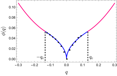
Figure 2: (color online) The ldf in (16) for the area under alive trajectories of a mortal Brownian particle with a death rate $\alpha=0.04$. The change of color at $q=\pm q_{c}$, where $q_{c}=\frac{2}{3}\sqrt{\alpha}$, signifies the second-derivative-discontinuity of $\phi(q)$ in (10). The data points indicate results from direct sampling using Monte Carlo simulation averaged over $4\times 10^{8}$ iterations for $T=300$ with $dt=0.01$. The extreme rarity of fluctuations for large $q$ values makes it difficult to sample beyond a certain range, for which specialized rare-even simulation methods [77] are required.

III.2 A general class of observables

The origin of the singularities in the ldfs for position and area lies in the competition between trajectories that remained alive for the entire duration and trajectories that died at an intermediate time. Such competition could result in similar singularities for other path-dependant observables. To illustrate this aspect, we consider a subset of observables $Q$ in (1) with $V(X_{t})=0$ while $U(X_{t})$ is a function of the alive part of trajectory $X_{t}$:

$$Q=\int_{0}^{t_{f}}dt\;U(X_{t})$$ (17)

where $t_{f}$ is the time until which the particle is alive.

We define $P_{T}(Q|x_{0})$ as the probability of the observable $Q$ at time $T$ for a mortal Brownian motion starting at $x_{0}$. Analogous to (8), the contributions to $P_{T}(Q|x_{0})$ are split into two classes of trajectories:

$$P_{T}(Q|x_{0})=P^{\text{(a)}}_{T}(Q|x_{0})+P^{\text{(d)}}_{T}(Q|x_{0})$$ (18)

where $P^{\text{(a)}}_{T}(Q|x_{0})$ is the contribution from the living trajectories, while $P^{\text{(d)}}_{T}(Q|x_{0})$ is the contribution from trajectories that died before time $T$. The two probabilities are related,

$$P^{\text{(d)}}_{T}(Q|x_{0})=\alpha\int_{0}^{T}dtP^{\text{(a)}}_{t}(Q|x_{0}).$$ (19)

For determining $P^{\text{(a)}}_{t}(Q|x_{0})$, we adopt a backward Fokker-Planck equation approach discussed in [62]. We define a double Laplace transformation

$$\mathcal{D}_{t\to s}^{Q\to p}\odot f_{t}(Q)=\int_{0}^{\infty}dte^{-st}\int dQ\;e^{pQ}f_{t}(Q).$$ (20)

Expressing (18) in terms of the transformed variables and using (19) gives

$$R_{s}(p,x_{0})=S_{s}(p,x_{0})+\frac{\alpha}{s}S_{s}(p,x_{0})$$ (21)

where $R_{s}(p,x_{0})$ and $S_{s}(p,x_{0})$ are the $\mathcal{D}$-transform of $P_{T}(Q|x_{0})$ and $P^{\text{(a)}}_{T}(Q|x_{0})$.

In line with the methods illustrated in [62], we find that $S_{s}(p,x_{0})$ is a solution of the ordinary differential equation

$$\frac{d^{2}S_{s}}{dx_{0}^{2}}-(\alpha+s-pU(x_{0}))S_{s}=-1.$$ (22a)

The specific boundary condition hinges on the observable in question. For observables where $$U(x)\to 0 x$$ for large ,

$$S_{s}(p,x_{0})=\frac{1}{\alpha+s}\qquad\textrm{for }x_{0}\to\pm\infty.$$ (22b)

In principle, obtaining a solution for $S_{s}(p,x_{0})$ allows us to compute $R_{s}(p,x_{0})$ in (21) and perform the inverse $\mathcal{D}$-transformation to derive the probability $P_{T}(Q|x_{0})$. However, performing these steps analytically for arbitrary $U(x)$ is not always feasible. Nevertheless, a large deviation form of the probability $P_{T}(Q|x_{0})$ can be deduced from the poles of $R_{s}(p,x_{0})$. This can be seen as follows. Assuming $P_{T}(Q=qT|x_{0})\sim e^{-T\phi(q)}$, the Laplace transformation

$$\int dQ\,e^{pQ}\,P_{T}(Q=qT)\sim e^{T\mu(p)}$$ (23)

for large $T$, where $\mu(p)$ is the scgf related to $\phi(q)$ by (5). An additional Laplace transformation gives

$$R_{s}(p,x_{0})\sim\frac{1}{s-\mu(p)}.$$ (24)

Therefore, a pole of $R_{s}(p,x_{0})$ at $s=\mu(p)$ suggests a large deviation asymptotic of $P_{T}(Q=qT|x_{0})$ where the ldf $\phi(q)$ is a Legendre-Fenchel transform (5) of $\mu(p)$. If $R_{s}(p,x_{0})$ has multiple poles, the scgf $\mu(p)$ is given by the maximum among all the poles.

This pole structure is seen in the ldf of $P_{t}(x)$ in (10), corresponding to $Q=x$ for which $U=0$ and $V=1$ in (1). Refering to (9), it is straightforward to demonstrate that the corresponding $R_{s}(p,0)=\frac{\alpha+s}{s\left(\alpha-p^{2}+s\right)}$, which has two poles at $s=0$ and at $s=p^{2}-\alpha$. (Here, $x_{0}=0$ is the initial position for this problem.) This results in the scgf, $\mu(p)=\max\{0,p^{2}-\alpha\}$; and its Legendre-Fenchel transform yields the ldf in (10).

In the following, we employ this general approach to obtain large deviations function for a couple of observables with singular ldf.

Remark: A crucial observation in this problem is that the slope $\sqrt{\alpha}$ of the linear part of the ldf in (10) for $|q|<2\sqrt{\alpha}$ corresponds to the pole of $sR_{s}(p,0)$ with respect to $p$ for vanishing $s$. This structure is more general. For an arbitrary $Q$, if the $P_{T}(Q|x_{0})$ is stationary within a range of $Q$ such that the ldf $\phi(q)=cq$, then the corresponding $sR_{s}(p,x_{0})$ for vanishing $s$ has a pole at $p=c$.

III.2.1 Local time

For $U(x)=\delta(x-a)$, the observable $Q$ corresponds to the local time density [81, 82], where $Qdx$ gives the net amount of time spent by the alive particle in the window $[a-\frac{dx}{2},a+\frac{dx}{2}]$ up to time $T$.

The solution for (22b) in this case is given by

$$S_{s}(p,x_{0})=\frac{1}{\alpha+s}\left\{1-\frac{p}{p-2\sqrt{\alpha+s}}e^{-|x_{0}-a|\sqrt{\alpha+s}}\right\}.$$ (25)

Substituting this into (21) reveals that $R_{s}(p,x_{0})$ has two poles, at $s=0$ and at $s=\frac{1}{4}p^{2}-\alpha$. Consequently

$$\mu(p)=\max\left\{0,\frac{p^{2}}{4}-\alpha\right\}.$$ (26)

The scgf in (26) has a singularity at $p=2\sqrt{\alpha}$. Performing a Legendre-Fenchel transformation of the scgf results in a singular ldf given by

$$\phi(q)=\begin{dcases}2q\sqrt{\alpha}&0\leq q<\sqrt{\alpha},\\ \alpha+q^{2}&q\geq\sqrt{\alpha}.\end{dcases}$$ (27)

This singularity is explicitly verified for $x_{0}=a$, for which the inverse-$\mathcal{D}$ transformation of $R_{s}(p,x_{0})$ can be analytically performed, yielding $P_{T}(Q|a)=\frac{1}{\sqrt{T}}h\left(\frac{Q}{\sqrt{T}},\sqrt{\alpha T}\right)$, where

$$h(x,y)= \frac{2e^{-x^{2}-y^{2}}}{\sqrt{\pi}}+$$

$$y\left(e^{-2xy}\textrm{erfc}(x-y)-e^{2xy}\textrm{erfc}(x+y)\right).$$ (28)

III.2.2 Residence time

Next example we consider is the time spent by the particle within an interval while it was alive. To keep the algebra simple, we consider a symmetric interval $-a\leq x\leq a$ with respect to the starting point $x_{0}=0$. The residence time is the observable (1) with $U(x)=1$ inside this interval and zero outside [83].

The solution to (22b) for this specific $U(x)$ is expressed as follows: for $x\in[-a,a]$,

$$S_{s}(p,x_{0})=\frac{1}{\widehat{p}}\left(-1+p\frac{\cos(x_{0}\sqrt{\widehat{p}})}{d(s,p)\sqrt{\widehat{s}}}\right)$$ (29)

and outside this region

$$S_{s}(p,x_{0})=\frac{1}{\widehat{s}}\left(1+p\frac{\sin(a\sqrt{\widehat{p}})e^{(a-|x_{0}|)\sqrt{\widehat{s}}}}{d(s,p)\sqrt{\widehat{p}}}\right)$$ (30)

where we denote $\widehat{p}=p-s-\alpha$, $\widehat{s}=s+\alpha$, and the denominator

$$d(s,p)=\sqrt{\widehat{s}}\cos(a\sqrt{\widehat{p}})-\sqrt{\widehat{p}}\sin(a\sqrt{\widehat{p}}).$$ (31)

Using this solution, the expression for $R_{s}(p,x_{0})$ in (21) can be written as

$$R_{s}(p,x_{0})=\frac{n(s,p,x_{0})}{s\;d(s,p)}$$ (32)

where the numerator is analytic in $s$, and the non-trivial poles for $R_{s}(p,x_{0})$ arise from the roots of $d(s,p)$.

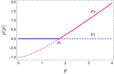
Figure 3: (color online) The solid line represents the scgf in (33) for the residence time in the interval $[-1,1]$ of a mortal Brownian particle with a death rate $\alpha=1$. The scgf is the maximum of the two poles: $\mu_{1}=0$ (blue) and $\mu_{2}(p)=s^{\star}(p)$ (pink) of $R_{s}$ in (32).

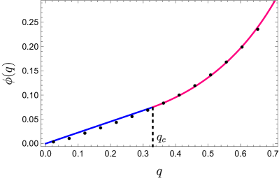
Figure 4: (color online) The ldf for residence time of a mortal Brownian particle with the same parameter values of Fig. 3. The solid line represents the theoretical result in (34) while the points indicate Monte Carlo results obtained by averaging over $10^{9}$ iterations with parameter values $\alpha=0.04,t=30$, $dt=0.01$. At the singular point $q_{c}$, marked by the dashed line, the $\phi^{\prime\prime}(q)$ is discontinuous. Improving numerical results requires the use of importance-sampling methods [77].

Following our argument discussed earlier, the scgf $\mu(p)$ is the largest non-negative root in $s$ for which $sd(s,p)=0$. It turns out that for $p$ less than a critical value $p_{c}$, defined as the positive solution of $d(0,p_{c})=0$, there are no positive roots $s^{\star}$ such that $d(s^{\star},p)=0$. In this scenario, the trivial pole $s=0$ in (32) gives the scgf $\mu(p)=0$. Altogether, this results in a singular scgf

$$\mu(p)=\begin{dcases}0&\textrm{for }0\leq p<p_{c}\\ s^{\star}(p)&\textrm{for }p_{c}\geq p.\end{dcases}$$ (33)

with $s^{\star}(p)$ and $p_{c}$ defined above.

The Legendre-Fenchel transformation (5) of the scgf in (33) results in the singular ldf

$$\phi(q)=\begin{dcases}p_{c}q&\textrm{for }0\leq q<q_{c},\\ \max\{pq-s^{\star}(p)\}&\textrm{for }q\geq q_{c},\end{dcases}$$ (34)

where $q_{c}=\partial_{p}s^{\star}(p_{c})$. The scgf (33) and the ldf (34) are plotted in Fig. 3 and Fig. 4, respectively, for specific parameter values.

IV Brownian Motion in presence of an absorbing boundary

In this second example, we examine a one-dimensional Brownian particle confined within an absorbing wall at the origin and a reflecting wall at $x=L$. As illustrative examples, we focus on a sub-class of path dependent observables given by (1), where $V(x)=0$ for all $x$.

Similar to (18), the contribution to the probability $P_{T}(Q|x_{0})$ of $Q$ for the particle starting at $x_{0}$ arises from two classes of trajectories:

$$P_{T}(Q|x_{0})=P^{\text{sur}}_{T}(Q|x_{0})+\int_{0}^{T}dtP^{\text{fp}}_{t}(Q|x_{0}),$$ (35)

where $P^{\text{sur}}_{T}(Q|x_{0})$ is the joint probability for the particle to survive up to time $T$ without being absorbed and contribute $Q$, while $P^{\text{fp}}_{t}(Q|x_{0})$ is the probability for the particle to get absorbed at time $t<T$ and contribute an amount $Q$ to the observable.

Applying double Laplace transformation (20) to (35) yields

$$R_{s}(p,x_{0})=S_{s}(p,x_{0})+\frac{1}{s}F_{s}(p,x_{0}),$$ (36)

where the terms are the $\mathcal{D}$-transform of respective probabilities in (35). Utilising a backward Fokker-Planck approach described in [62], we find that $S_{s}(p,x_{0})$ is a solution of the ordinary differential equation

$$\frac{d^{2}S_{s}}{dx_{0}^{2}}-(s-pU(x_{0}))S_{s}=-1$$ (37a)

with the boundary conditions

$$S_{s}(p,0)=0\quad\textrm{and }\frac{dS}{dx_{0}}\bigg{|}_{x_{0}=L}=0.$$ (37b)

Similarly, $$F_{s}(p,x_{0})$$ satisfies the following ordinary differential equation:

$$\frac{d^{2}F_{s}}{dx_{0}^{2}}-(s-pU(x_{0}))F_{s}=0$$ (38a)

with the boundary conditions

$$F_{s}(p,0)=1\quad\textrm{and }\frac{dF_{s}}{dx_{0}}\bigg{|}_{x_{0}=L}=0.$$ (38b)

As we discussed in Section. III.2, the presence of a pole for $R_{s}(p,x_{0})$ at $s=\mu(p)$ implies a large deviation form of the probability $P_{T}(Q|x_{0})$, where the ldf $\phi(q)$ relates to the scgf $\mu(p)$ through a Legendre-Fenchel transformation (5).

In the following, we apply this general approach to derive ldfs for two observables considered in Section. III.2.

IV.1 Local time

For $U(x)=\delta(x-a)$ with $0<a<L$, the observable $Q$ in (1) is the local time density. For this observable, the solutions for $S_{s}$ and $F_{s}$ in (37b, 38b) are straightforward and are expressed as

$$S_{u^{2}}(p,x_{0})=\frac{n_{1}(u,p,x_{0})}{d(u,p)},\quad F_{u^{2}}(p,x_{0})=\frac{n_{2}(u,p,x_{0})}{d(u,p)}$$ (39)

where both the numerators (expressions given in the appendix D) and the common denominator

$$d(u,p)=p\sinh\left(au\right)\cosh\left(u(L-a)\right)+u\cosh\left(Lu\right)$$ (40)

are analytic functions of $u$. Using these solutions in (36), we obtain

$$R_{u^{2}}(p,x_{0})=\frac{u^{2}n_{1}(u,p,x_{0})+n_{2}(u,p,x_{0})}{u^{2}d(u,p)}.$$ (41)

For $p$ exceeding a critical value $p_{c}=1/a$, the denominator $d(u,p)$ has real roots at non-zero $u=\pm u_{c}(p)$. Consequently, $R_{s}(p,x_{0})$ features a pole at positive $s=u_{c}(p)^{2}$ for $p>p_{c}$.

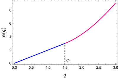
Figure 5: (color online) The ldf (42b) for local time at $a=1/2$ for a Brownian particle confined between an absorbing wall at the origin and a reflecting wall at $L=1$. At the singular point $q_{c}$, marked by the dotted line, the $\phi^{\prime\prime}(q)$ is discontinuous. The inset shows the corresponding scgf given in (42a).

For $p<p_{c}$, the denominator $d(u,p)$ has no real roots in $u$, and consequently, $R_{s}(p,x_{0})$ lacks a pole at $s>0$. In this case, the leading contribution to the scgf arises from the real pole at $s=0$.

Altogether, this yields the piece-wise scgf

$$\mu(p)=\begin{dcases}0&p<1/a\\ u_{c}(p)^{2}&p\geq 1/a\end{dcases}$$ (42a)

where $$u_{c} d(u_{c},p)=0$$ is the largest real solution of the transcendental equation in (40).

A Legendre-Fenchel transformation (5) leads to the ldf

$$\phi(q)=\begin{dcases}\frac{1}{a}q&q<q_{c}\\ \max_{p}\{qp-u_{c}^{2}(p)\}&q\geq q_{c}\end{dcases}$$ (42b)

with $q_{c}=\mu^{\prime}(p_{c}^{+})$ where the derivative is evaluated on the right side of $p_{c}$. The singular ldf and the corresponding scgf are plotted in Fig. 5.

Remark: The linear ldf for $q<q_{c}$ implies a stationary regime for the $P_{T}(Q|x_{0})$. As discussed in Section. III.2, the slope $1/a$ for the ldf in this regime can also be observed from the pole of $sR_{s}(p,x_{0})$ at $p=1/a$ for vanishing $s$.

IV.2 Residence time

The residence time is defined by the observable $Q$ in (1) with $V(x)=0$ for all $x$, while $U(x)=1$ in the interval $x\in[a,b]$ for $0<a<b<L$, zero outside this interval. The solution for the corresponding $S$ and $F$ in (37b, 38b) is straightforward but cumbersome to write in the main text. (For their explicit solution, refer to the supplemental Mathematica notebook [84].) The solution follows the structure of (39), with a denominator

$$\begin{split}&d_{\text{res}}(u,p)=\left(p-2u^{2}\right)\tanh\left(u(a-b+L)\right)\\ &+\frac{p\sinh\left(u(a+b-L)\right)}{\cosh\left(u(a-b+L)\right)}+\frac{2u\sqrt{(p-u^{2})}}{\tan((a-b)\sqrt{p-u^{2}})}.\end{split}$$ (43)

The subsequent analysis parallels that of the local time discussed in the previous section. The scgf has similar formal structure as in (33), where $u_{c}$ is the largest positive root of $d_{\text{res}}(u,p)$. This root exists above a non-zero threshold value of $p_{c}$, which is obtained by $d_{\text{res}}(0,p_{c})=0$ (refer to the discussion above (33)). The resulting scgf and the corresponding ldf are shown in Fig. 6.

Remark: Singular scgf is not limited to the finite domain of the Brownian motion. When the reflecting boundary is pushed to infinity ($L\to\infty$), from (43) we get that $\mu(p)$ is the largest non-negative solution $s$ of the transcendental equation

$$\frac{2\sqrt{s(p-s)}}{\tan\left((a-b)\sqrt{p-s}\right)}=2s-p\left(1-e^{-2a\sqrt{s}}\right)$$ (44)

Resulting scgf and the corresponding ldf have similar singular structure as in Fig. 6. Effect of conditioning on Brownian motion in a similar geometry has been recently studied in [85].

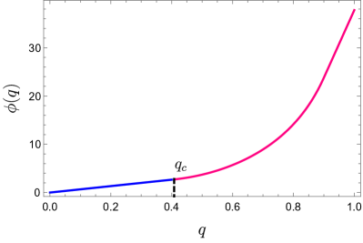
Figure 6: (color online) The ldf for residence time of a Brownian particle in the interval $[1/3,2/3]$, confined between an absorbing wall at the origin and a reflecting wall at $L=1$. At the singular point $q_{c}$, marked by the dotted line, the $\phi^{\prime\prime}(q)$ is discontinuous. The inset shows the corresponding scgf.

V Spectral method

The problem of the long-time asymptotics (3) of the probability $P(Q)$ of empirical observables (1) can be approached using an alternative method that has recently gained considerable attention [57, 58, 59, 60, 61]. In this approach, large deviations are expressed in terms of largest eigenvalue of an operator, offering an intuitive analogy with free-energy calculations using the transfer matrix method [67, 68, 69].

We present a brief introduction to this method using the simplest example of a standard Brownian motion $\dot{X}_{t}=\eta_{t}$ with Gaussian white noise $\eta_{t}$ of mean zero and covariance of $\langle\eta_{t}\eta_{t^{\prime}}\rangle=2\delta(t-t^{\prime})$. For the joint probability $P_{T}(Q,x_{T}|x_{0})$ of the observable $Q$ in (1) and the final position $x_{T}$, starting at $x_{0}$, the generating function

$$R_{T}(p,x_{T}|x_{0})=\int dQe^{pQ}P_{T}(Q,x_{T}|x_{0})$$ (45)

has a path integral representation [62],

$$R_{T}(p,x_{T}|x_{0})=\int_{x_{0}}^{x_{T}}\mathcal{D}[x_{t}]e^{-S_{T}(x_{t})}$$ (46)

where the Feynman-Kac action

$$S_{T}(x_{t})=\int_{0}^{T}dt\,\left\{\frac{\dot{x}_{t}^{2}}{4}-p\dot{x}_{t}V(x_{t})-pU(x_{t})\right\}$$ (47)

is analogous to the action of a charged particle in an electromagnetic field. The corresponding analogue of the Schrodinger equation is the Feynman-Kac formula [62]

$$\frac{d}{dT}R_{T}(p,x|x_{0})=\mathcal{L}_{p}\cdot R_{T}(p,x|x_{0})$$ (48a)

where the operator

$$\mathcal{L}_{p}=\left(\frac{d}{dx}-pV\right)^{2}+pU.$$ (48b)

is often referred to as the tilted operator [57, 58, 59, 60, 61].

If the operator $\mathcal{L}_{p}$ has a spectral gap between its largest and the second-largest eigenvalues, then for large $T$, $R_{T}(p,x_{T}|x_{0})\simeq e^{T\mu(p)}r_{p}(x_{T})\ell_{p}(x_{0})$, where $\mu(p)$ is the largest eigenvalue of $\mathcal{L}_{p}$ with the associated left eigenvector $\ell_{p}(x)$ and right eigenvector $r_{p}(x)$ satisfying

$$\mathcal{L}^{\dagger}_{p}\ell_{p}(x)=\mu(p)\ell_{p}(x)\textrm{ ~~ and }\mathcal{L}_{p}r_{p}(x)=\mu(p)r_{p}(x),$$ (49)

respectively, where $\dagger$ denotes the adjoint. Comparing the asymptotics of $R_{T}(p,x_{T}|x_{0})$ with the asymptotics (4) one can recognise that the largest eigenvalue $\mu(p)$ gives the scgf of $Q$.

For a strictly convex $\mu(p)$, the asymptotic for $R_{T}(p,x_{T}|x_{0})$ corresponds [61] to the large $T$ asymptotic of the joint probability

$$P_{T}(Q=qT,x_{T}|x_{0})\simeq\sqrt{\frac{\phi^{\prime\prime}(q)}{2\pi T}}e^{-T\phi(q)}r_{p}(x_{T})\ell_{p}(x_{0})$$ (50a)

with

$$\phi(q)=pq-\mu(p)\quad\textrm{and }\mu^{\prime}(p)=q,$$ (50b)

which is seen by a saddle point approximation of the integral in (45).

The relation (50b) is an explicit version of (5) for a strictly convex $\mu(p)$. It establishes an equivalence between the conditioned ensemble and the ensemble where evolution is weighted by the value of the observable. Such equivalence of ensemble also extends to the dynamics [57, 58, 59, 60, 61], more precisely, to the joint probability $P_{t}(Q,x|x_{T},x_{0})$ of being at location $x$ at an intermediate time $0<t<T$, starting at $x_{0}$ and ending at $x_{T}$, and yielding a value $Q$ for the empirical observable (1) measured over the time window $[0,T]$. Analogous to (50), the joint probability can be estimated in the large time $T$ limit by the asymptotics of the corresponding generating function $G_{t}(p,x|x_{T},x_{0})$, defined in a way similar to (45). This further implies [57, 58, 59, 60, 61] that the conditional probability

$$P_{t}(x|Q,x_{T},x_{0})=\frac{P_{t}(Q,x|x_{T},x_{0})}{\int dxP_{t}(Q,x|x_{T},x_{0})}$$ (51)

can be estimated in the large $T$ limit by an analogous quantity in the weighted ensemble,

$$P_{t}(x|Q=qT,x_{T},x_{0})\simeq\frac{G_{t}(p,x|x_{T},x_{0})}{\int dxG_{t}(p,x|x_{T},x_{0})}$$ (52)

with $p$ and $q$ related by (50b).

To describe the dynamics followed by the conditional probability $P_{t}(x|Q,x_{T},x_{0})$, we follow a procedure similar to that described in [63] for conditioned dynamics of a Brownian bridge. Using Markovianity,

$$G_{t}(p,x|x_{T},x_{0})=R_{T-t}(p,x_{T}|x)R_{t}(p,x|x_{0})$$ (53)

where $R_{t}(p,x|x_{0})$ evolves according to (48a) with $T$ replaced by $t$, and $R_{T-t}(p,x_{T}|x)\equiv B_{t}(p,x|x_{T})$ follows the backward evolution [62]

$$-\frac{d}{dt}B_{t}(p,x|x_{T})=\mathcal{L}^{\dagger}\cdot B_{t}(p,x|x_{T}).$$ (54)

It then requires a straightforward algebra to show that $G_{t}(p,x|x_{T},x_{0})$ in (53) satisfies

$$\frac{dG_{t}}{dt}=-2\frac{d}{dx}\left\{\left(pV(x)+\frac{1}{B_{t}}\frac{dB_{t}}{dx}\right)G_{t}\right\}+\frac{d^{2}G_{t}}{dx^{2}}.$$ (55)

Integrating the above equation over $x$, we see that the denominator in (52) is independent of time, assuming that $G_{t}(p,x|x_{T},x_{0})$ vanishes sufficiently quickly for $x\to\pm\infty$. Using these results in (52), it immediately follows that the effective dynamics of the conditional probability $P_{t}(x|qT,x_{T},x_{0})$ is similar to (55), with $p$ and $q$ related by (50b).

The effective dynamics particularly simplifies for $1\ll t\ll T$, where, for typical observables, the system reaches a quasi-stationary state [57, 58, 59, 60, 61], in which the conditional probability $P_{t}(x|qT,x_{T},x_{0})\simeq P_{t}(x|q)$ is independent of $x_{T}$, $x_{0}$, and $T$. Moreover, $B_{t}(p,x|x_{T})\simeq e^{-t\mu(p)}\ell_{p}(x)r_{p}(x_{T})$. The resulting conditioned dynamics is a drifted Brownian motion [57, 58, 59, 60, 61] governed by the Fokker-Planck equation

$$\frac{d}{dt}P_{t}(x|q)=-\frac{d}{dx}\Big{(}F_{t}(x,p)P_{t}(x|q)\Big{)}+\frac{d^{2}}{dx^{2}}P_{t}(x|q)$$ (56a)

with a modified force

$$F_{t}(x,p)=2\left\{pV(x)+\frac{\ell_{p}^{\prime}(x)}{\ell_{p}(x)}\right\}$$ (56b)

where the left eigenvector $\ell_{p}(x)$ is defined in (49), and the parameters $p$ and $q$ are related by (50b). This effective description for the conditioned dynamics suitably generalizes [57, 58, 59, 60, 61] for general diffusive processes and for Markov processes on discrete states and time.

In this spectral method, singularities in $\mu(p)$ can arise from crossing of the two leading eigenvalues, denoted as $\mu_{1}(p)$ and $\mu_{2}(p)$, of the tilted operator $\mathcal{L}_{p}$ in (48b), such that the scgf $\mu(p)=\max\{\mu_{1}(p),\mu_{2}(p)\}$. This is analogous to the origin of singular free energy at the phase transition point of equilibrium lattice models from the crossing of leading eigenvalues of the associated transfer matrix [67, 68, 69]. Across the singular point, the largest eigenvector also changes abruptly indicating a sudden change in the effective dynamics (56b). This way the singularity of scgf $\mu(p)$ and equivalently that of the ldf $\phi(q)$ corresponds to a phase transition in the system’s dynamics as the condition on the observable value is varied.

We illustrate how the DPTs for the models we discussed in Section. III and Section. IV can be described using the spectral method. Our discussion will focus on the residence time for the two models; however, the analysis for the other observables follows a similar analysis.

V.1 Residence time for a Brownian motion in presence of an absorbing wall

We initiate our discussion by revisiting the residence time problem, studied in Section. IV.2, of a Brownian particle in presence of an absorbing and a reflecting walls at $x=0$ and $x=L$ respectively. Here, we reproduce our earlier results using the spectral method, with the observable under consideration being the residence time in the interval $x\in[a,b]$ with $0<a<b<L$.

From the previous section (48b), we see that the titled operator in this example takes the form

$$\mathcal{L}_{p}=\frac{d^{2}}{dx^{2}}+p\,\mathbb{1}_{[a,b]}.$$ (57)

The scgf, $\mu(p)$, for the residence time is given by the largest eigenvalue of $\mathcal{L}_{p}$. Here, the operator has an eigenvalue $\mu_{1}(p)=0$ for all $p$ and an associated left eigenfunction denoted by $\ell_{p}^{(1)}(x)$. For $p=0$, this eigenvalue corresponds to the empty stationary state due to the absorbing wall, for which the left eigenfunction $\ell_{0}^{(1)}(x)=1$. Note that this eigenfunction does not vanish at the absorbing wall. The second relevant eigenvalue $\mu_{2}(p)$ is the largest eigenvalue of $\mathcal{L}_{p}$ with a vanishing boundary condition $\ell_{p}^{(2)}(0)=0$ for the corresponding eigenfunction $\ell_{p}^{(2)}(x)$ at the absorbing wall. On the reflecting wall at $x=L$, both eigenfunctions, $\ell_{p}^{(1)}(x)$ and $\ell_{p}^{(2)}(x)$, satisfy the zero gradient condition $\ell_{p}^{(1)\prime}(L)=0$ and $\ell_{p}^{(2)\prime}(L)=0$ [86]. In Appendix A, we discuss an origin of the absorbing boundary condition.

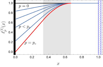
Figure 7: (color online) The left eigenfunction $\ell^{(1)}_{p}(x)$ in (58) corresponding to the vanishing eigenvalue $\mu(p)=0$ for different values of $p$ and a fixed set of parameters $a=1/3$, $b=2/3$, $L=1$. At a critical value $p=p_{c}$, the eigenfunction $\ell^{(1)}_{p}(x)$, indicated in red, vanishes at the absorbing boundary $x=0$.

Figure 8: (color online) The left eigenfunction $\ell^{(2)}_{p}(x)$ in (59) with the absorbing boundary condition at $x=0$ for identical set of parameter values of $a$, $b$, and $L$ as in Fig. 7. At a critical value $p=p_{c}$, the eigenfunction $\ell_{p}(x)$, indicated in red, is constant for $x>b$.

V.1.1 Zero eigenvalue problem

The left eigenfunction $\ell^{(1)}_{p}(x)$ corresponding to the zero eigenvalue $\mu_{1}(p)=0$ with the reflecting boundary condition $\ell^{(1)\prime}_{p}(L)=0$ is a piece-wise function

$$\ell^{(1)}_{p}(x)=\begin{cases}A_{1}+A_{2}x&\textrm{for }0<x<a\\ B_{1}\sin(\omega x)+B_{2}\cos(\omega x)&\textrm{for }x\in[a,b]\\ 1&\textrm{for }b<x<L\end{cases},$$ (58)

where $\omega^{2}=p$ and $A_{1},A_{2},B_{1}$, and $B_{2}$ are $p$-dependent constants determined by continuity of $\ell^{(1)}_{p}(x)$ and its derivative. The eigenfunction is plotted in Fig. 7 for a set of values of the tilting parameter $p$. Notably, $\ell^{(1)}_{0}(x)=1$, which is the left eigenfunction associated with the stationary state of a Markov operator. It is worth mentioning that the eigenfunction does not necessarily vanish at the absorbing wall $x=0$.

V.1.2 Eigenvalue-problem with absorbing boundary condition

The eigenvalue problem for $\mu_{2}(p)$ and its associated left eigenfunction $\ell^{(2)}_{p}(x)$, with the absorbing boundary condition $\ell^{(2)}_{p}(0)=0$ and reflecting boundary condition $\ell_{p}^{(2)\prime}(L)=0$, is analogous to the quantum mechanical problem with infinite potential at origin, a square-well potential in $a<x<b$, and a zero current condition at $x=L$. The solution is given by

$$\ell^{(2)}_{p}(x)=\begin{cases}e^{\kappa x}-e^{-\kappa x}&0<x<a\\ D_{1}\sin(\gamma x)+D_{2}\cos(\gamma x)&x\in[a,b]\\ E\left(e^{\kappa(x-L)}+e^{-\kappa(x-L)}\right)&b<x<L\end{cases},$$ (59)

where $\kappa=\sqrt{\mu_{2}(p)}$, $\gamma=\sqrt{p-\mu_{2}(p)}$, and the $p$-dependent coefficients $D_{1}$, $D_{2}$ and $E$ are determined from continuity of the eigenfunction and its derivative. The eigenvalue $\mu_{2}(p)$ is a solution of the transcendental equation

$$\frac{v+u\tan(v(b-a))\tanh(u(L-b))}{v\{v\tan(v(b-a))-u\tanh(u(L-b))\}}=\frac{\tanh(au)}{u}$$ (60)

where $u^{2}=\mu_{2}(p)$ and $v^{2}=p-\mu_{2}(p)$. The eigenfunction $\ell_{p}^{(2)}(x)$ is illustrated in Fig. 8 for a range of tilting parameters $p$ above a critical value $p_{c}$ defined by the solution of (60) for $\mu_{2}(p_{c})=0$.

As in the previous example, the crossing of the two eigenvalues, $\mu_{1}(p)=0$ and $\mu_{2}(p)$, gives rise to a non-analytic scgf, which in turn results in a non-analytic ldf. These findings match with those obtained in Section. IV.2.

V.1.3 Conditioned dynamics

The singularity of the ldf can be attributed to abrupt change in the conditioned dynamics. Referring back to the discussion at the beginning of Section. V and (56b), the restricted ensemble of trajectories spending a fraction of time $q=\mu^{\prime}(p)$ in the region $[a,b]$, can be described as a Brownian motion inside a potential

$$U_{p}(x)=-2\ln\ell_{p}(x).$$ (61)

For $p>p_{c}$, where the scgf is $\mu_{2}(p)$, the eigenfunction $\ell_{p}^{(2)}(x)$ gives a potential (see Fig. 9) that diverges at $x=0$ and consequently, the trajectories never reach the absorbing site. As $q\to 1$, $\ell_{p}^{(2)}(x)\to 0$ for $x$ outside $[a,b]$ resulting in a confining potential $U_{p}(x)$ around the interval $[a,b]$.

For $p<p_{c}$, where the scgf $\mu(p)=0$, the relation $q=\mu^{\prime}(p)$ yields a constant value for $q$. This indicates a breakdown of ensemble equivalence, rendering the construction [61] of effective dynamics inapplicable. Further discussions on this can be found in [48]. Nevertheless, it is evident that the conditioned dynamics for $p>p_{c}$ do not extend to $p<p_{c}$, indicating a sudden change of the dynamics at the transition point $p=p_{c}$.

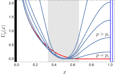
Figure 9: (color online) The effective potential corresponding to the eigenfunction $\ell_{p}^{(2)}(x)$ for the dynamics of a Brownian particle confined between an absorbing wall at the origin and a reflecting wall at $x=1$, conditioned to yield a value of residence time $Q=T\mu^{\prime}(p)$. The plot is for a choice of parameter values $a=1/3,b=2/3$, and $L=1$.

V.2 Residence time for mortal Brownian motion

We now return to the problem discussed in Section. III.2.2: Brownian particle subjected to a constant death rate, with the observable being the total time spent within an interval $x\in[-a,a]$. Once again, the scgf, $\mu(p)$, of the residence time is given by the largest eigenvalue of the corresponding tilted operator.

Adhering to the framework elucidated in [61], it can be shown that the pertinent tilted operator for this problem takes the form of

$$\mathcal{L}_{p}=\begin{pmatrix}0&\alpha\\ 0&\widehat{\mathcal{L}}_{p}\end{pmatrix}.$$ (62)

where

$$\widehat{\mathcal{L}}_{p}=\frac{d^{2}}{dx^{2}}-\alpha+p\mathbb{1}_{[-a,a]}.$$ (63)

In writing $\mathcal{L}_{p}$, we separated the configuration space based on whether the particle is alive or dead. The dead particle is immobile and does not contribute to our observables. Consequently, a dead particle is assigned a single configuration by ignoring its position degrees of freedom.

The scgf, $\mu(p)$, for the residence time is given by the largest eigenvalue of $\mathcal{L}_{p}$. In this context, there are two distinct relevant eigenvalues. One of them is $\mu_{1}(p)=0$ for all $p$ associated to the left eigenvector $\begin{pmatrix}1&\ell^{(1)}_{p}(x)\end{pmatrix}$, with

$$\ell^{(1)}_{p}(x)=\begin{dcases}1+Ae^{\sqrt{\alpha}x}&\textrm{for }x<-a\\ B\cosh(x\sqrt{\alpha-p})+\frac{\alpha}{\alpha+p}&\textrm{for }x\in[-a,a]\\ 1+Ae^{-\sqrt{\alpha}x}&\textrm{for }x>a,\end{dcases}$$ (64)

where the constants $A$ and $B$ are determined by the continuity of $\ell^{(1)}_{p}(x)$ and its derivative. It is noteworthy that, for $p=0$, $\ell^{(1)}_{0}(x)=1$ which is consistent with the unit left eigenvector corresponding to zero eigenvalue of a Markov operator.

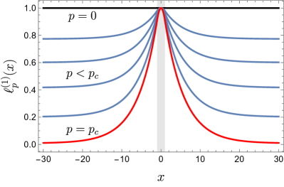
Figure 10: (color online) The normalized functional component of the eigenvector $\begin{pmatrix}1&\ell^{(1)}_{p}(x)\end{pmatrix}$ corresponding to the eigenvalue $\mu(p)=0$ of the operator $\mathcal{L}_{p}$ is depicted for various values of $p<p_{c}$. The normalization is such that the maximum value is set to $1$. The function normalized for $p=p_{c}$, highlighted in red, asymptotically vanishes for $x\pm\infty$. The parameters used are $a=1$ and $\alpha=0.04$, while the shaded gray region indicates the interval $-1<x<1$.

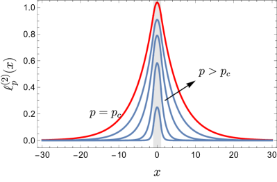
Figure 11: (color online) The function $\ell_{p}^{(2)}(x)$ in (67) is a component of the eigenvector $\begin{pmatrix}0&\ell^{(2)}_{p}(x)\end{pmatrix}$ associated with the eigenvalue $\mu_{2}(p)$ in (65) of the operator $\mathcal{L}_{p}$ in (62) for the same set of parameter values used in Fig. 10. The function is plotted for different values of $p\geq p_{c}$. The red solid line represents the function for $p=p_{c}$. The gray region indicates the interval $-1<x<1$.

The second eigenvalue, $\mu_{2}(p)$, corresponds to the eigenvector $\begin{pmatrix}0&\ell^{(2)}_{p}(x)\end{pmatrix}$, where $\ell^{(2)}_{p}(x)$ is the left eigenfunction corresponding to the largest eigenvalue $\mu_{2}(p)$ of $\widehat{\mathcal{L}}_{p}$. The operator in (63) is related by a similarity transformation to the tilted operator for residence time of a drifted BM [48]. It is also analogous to the quantum Hamiltonian for a particle in a finite potential well. This quantum analogy straightforwardly gives the largest eigenvalue of $\widehat{\mathcal{L}}_{p}$ written as

$$\mu_{2}(p)=\lambda(p)-\alpha.$$ (65)

where $\lambda(p)$ is the largest solution to the transcendental equation

$$\zeta=\gamma\tan(\gamma a)$$ (66)

with $\zeta=\sqrt{\lambda(p)}$ and $\gamma=\sqrt{p-\lambda(p)}$. The corresponding left eigenfunction is

$$\ell^{(2)}_{p}(x)=\begin{cases}e^{\zeta x}&\textrm{for }x<-a\\ C\cos(\gamma x)&\textrm{for }x\in[-a,a]\\ e^{-\zeta x}&\textrm{for }x>a.\end{cases}$$ (67)

with the parameter $C$ determined from the continuity condition at $x=\pm a$.

The scgf $\mu(p)$ for the residence time is the largest among the two eigenvalues: $\mu_{1}(p)=0$ and $\mu_{2}(p)$, which cross each other at a critical value $p=p_{c}$, reproducing the piece-wise function in (33) and consequently, the associated ldf in (34). (We have explicitly verified the agreement with the result in (33).) The value of $p_{c}$ can be determined by setting $\lambda(p_{c})=\alpha$ in (66), for which $\mu_{2}(p_{c})$ in (65) becomes zero.

The eigenvectors associated with the leading eigenvalues, $\mu_{1}(p)$ and $\mu_{2}(p)$, in their respective domains, are shown in Fig. 10 and Fig. 11, respectively, for a range of tilting parameters $p$.

Conditioned dynamics

As in the previous example, the singularity of the ldf here is due to the abrupt change in the conditioned dynamics. Beyond a critical value $p_{c}$, where the scgf is given by the eigenvalue $\mu_{2}(p)$, the effective mortality rate vanishes. This is seen from the vanishing component of the eigenvector $\begin{pmatrix}0&\ell^{(2)}_{p}(x)\end{pmatrix}$ in the effective transition rates constructed by comparing $\mathcal{L}_{p}$ in (62) with the tilted matrix of a discrete-state Markov process discussed in [61]. As a result, the effective dynamics resembles that of a standard Brownian motion conditioned to spend $q=Q/T$ fraction of time in the interval $[-a,a]$, which, following (56b), is described by a Brownian motion inside an effective potential

$$U_{p}(x)=-2\ln\ell_{p}^{(2)}(x)$$ (68)

with $\ell_{p}^{(2)}(x)$ in (67). The bias parameter $p$ is related to the observable’s value by the ensemble equivalence relation $q=\mu^{\prime}(p)$. The vanishing of $\ell_{p}^{(2)}(x)$ for large $x$ (see Fig. 11) results in a confining potential $U_{p}(x)$ around the interval $[-a,a]$, which gets narrower as $q\to 1$. For $p<p_{c}$, the ensemble equivalence breaks down and the construction of the effective dynamics in [61] does not apply.

VI Markov Chains

The origin of DPTs, as discussed in our examples of Langevine processes, is relatively easier to comprehend in their discrete counterparts, which are discrete time Markov processes on a finite configuration space. For a Markov chain, evolution of the probability $P_{t}(C)$ of a configuration $C$ at time $t$ is governed by

$$P_{t+1}(C^{\prime})=\sum_{C}M(C^{\prime},C)P_{t}(C),$$ (69)

where $M(C^{\prime},C)$ denotes the transition probability from state $C$ to $C^{\prime}$. A discrete analogue [61] of the empirical observable (1) is

$$Q=\sum_{t=0}^{T-1}f(C_{t})+\sum_{t=0}^{T-1}g(C_{t+1},C_{t}),$$ (70)

where $f(C)$ and $g(C,C^{\prime})$ are arbitrary functions. For instance, the residence time at a configuration $C$ corresponds to $f(C_{t})=\delta_{C_{t},C}$ and $g(C_{t+1},C_{t})=0$, while $f(C_{t})=0$ and $g(C_{t+1},C_{t})=\delta_{C_{t},C}\delta_{C_{t+1},C^{\prime}}$ gives the total number of jumps from configuration $C$ to $C^{\prime}$.

In the limit of large $T$, the probability of $Q$ has the asymptotic (2) with the corresponding scgf $\mu(p)$ in (4) relating to the largest eigenvalue $e^{\mu(p)}$ of the tilted matrix [57, 58, 59, 60, 61]:

$$M_{p}(C,C^{\prime})=M(C,C^{\prime})e^{p[f(C^{\prime})+g(C,C^{\prime})]},$$ (71)

which is a discrete analogue of the tilted operator (48b).

Analogous to (56b), the dynamics conditioned to yield a value of $Q_{T}$, in the large time limit, are described (excluding the non-quasi-stationary regimes near $t=0$ and $t=T$) by an effective Markov chain [57, 58, 59, 60, 61]:

$$P_{t+1}^{(p)}(C^{\prime})=\sum_{C}W_{p}(C^{\prime},C)P_{t}^{(p)}(C),$$ (72)

with the transition matrix

$$W_{p}(C^{\prime},C)=\frac{L_{p}(C^{\prime})}{e^{\mu(p)}L_{p}(C)}M_{p}(C^{\prime},C),$$ (73)

where $L_{p}$ is the left eigenvector of $M_{p}$ corresponding to the eigenvalue $e^{\mu(p)}$. The tilting parameter $p$ is expressed in terms of the observable value $Q_{T}$ by the relation $\mu^{\prime}(p)=Q_{T}/T$ [57, 58, 59, 60, 61].

In this formalism, the crossing of two leading eigenvalues of $M_{p}$ results a singular scgf and, consequently, an abrupt change in the effective transition matrix $W_{p}$. This draws an instructive analogy between DPTs and conventional equilibrium phase transitions relating to crossing of two largest eigenvalues of transfer matrix [69]. There are known examples of eigenvalue crossings in the transfer matrix of one-dimensional models [69, 87]. Notably, the transfer matrices in these examples are reducible and therefore do not satisfy the criteria for the Perron-Frobenius theorem [69]. In the following examples, we shall illustrate that the DPTs in non-ergodic Markov chains share similar characteristics, arising from the reducibility of the corresponding tilted matrices (71).

VI.1 Residence time in a three-state Markov chain

An example of a three state Markov chain is shown in Fig. 12. The corresponding transition matrix is

$$M=\begin{pmatrix}1&1-2r&1-2r\\ 0&r&r\\ 0&r&r\\ \end{pmatrix}.$$ (74)

The observable we consider is the residence time in the state 1, which corresponds to $f(C)=\delta_{C,\textbf{1}}$ and $g=0$ in the definition (70).

The tilted matrix (71) for this observable

$$M_{p}=\begin{pmatrix}1&(1-2r)e^{p}&1-2r\\ 0&re^{p}&r\\ 0&re^{p}&r\\ \end{pmatrix}.$$ (75)

has three eigenvalues: $e_{1}=1$, $e_{2}=r(1+e^{p})$, and $e_{3}=0$. The left eigenvectors of the dominant eigenvalues $e_{1}$ and $e_{2}$ are

$$v_{1}=\begin{pmatrix}\dfrac{1-r-re^{p}}{1-2r}&e^{p}&1\end{pmatrix}$$ (76)

and $v_{2}=\begin{pmatrix}0&e^{p}&1\end{pmatrix}$, respectively.

Figure 12: (color online) A three-state Markov chain with one absorbing state denoted by 0. The arrows indicate the allowed transitions with the corresponding transition probabilities. The residence time is measured at the state 1 (shaded in blue).

The scgf is given by the logarithm of the largest among the three eigenvalues, leading to

$$\mu(p) =\max\{0,\ln(r(1+e^{p}))\}$$ (77)

and its Legendre-Fenchel transformation (5) gives the piece-wise ldf

$$\phi(q) =\begin{dcases}q\ln\left(\frac{1-r}{r}\right)&\textrm{for }0\leq q\leq q^{\star}\\ q\ln\left(\frac{q}{1-q}\right)-\ln\left(\frac{r}{1-q}\right)&\textrm{for }q^{\star}<q\leq 1\end{dcases}$$ (78)

where $q^{\star}=1-r$. The ldf in (78) can alternatively be obtained, without the spectral method, using combinatorics followed by saddle point approximation. The shape of this ldf is qualitatively similar to the ldf in Fig 6 for the residence time of the Brownian motion in presence of an absorbing site.

The transition rates of the effective Markov process (73) for tilting parameter $p>p_{c}$ are expressed in terms of the eigenvector of the dominant eigenvalue and sketched in Fig. 13. However, for $p<p_{c}$, ensemble equivalence breaks down, rendering the construction of effective dynamics in [61] inapplicable.

Figure 13: (color online) Effective Markov processes for $p>p_{c}$ obtained using (73). In this scenario, the Markov process effectively behaves as if the absorbing site is not present, and the Markov trajectories do not evolve into it.

Remark: The two-state version of this problem was studied in [17], where, although the scgf was non-analytic, the ldf $\phi(q)$ was found to be linear across the entire allowed range of $q$.

VI.2 Integrated current in a four-state Markov chain

The Markov chain in consideration is illustrated in Fig. 14. This example serves a simple discrete analogue of the mortal Brownian motion considered in III, where the recurrent state is equivalent to the immobile dead state of the Brownian.

Figure 14: A four state Markov chain featuring a single recurrent state $\mathbfcal{R}$ and a transient state space $\mathbfcal{T}$ consisting of three states. In $\mathbfcal{T}$, any transient state has a probability $1-3r$, with $r<\frac{1}{3}$, to escape to $\mathbfcal{R}$. For jumps within $\mathbfcal{T}$ the transition probability is $r$ as indicated by arrows.

The observable we consider is the integrated current $Q$ in $T$-time steps counted by adding $1$ for each clockwise jump and subtracting $1$ for an anti-clockwise jump within $\mathcal{T}$. Jumps to $\mathcal{R}$ or to remain at the same site do not contribute to $Q$. The tilted matrix (71) for this observable is

$$M_{p}=\begin{pmatrix}1&1-3r&1-3r&1-3r\\ 0&r&r\mathrm{e}^{-p}&r\mathrm{e}^{p}\\ 0&r\mathrm{e}^{p}&r&r\mathrm{e}^{-p}\\ 0&r\mathrm{e}^{-p}&r\mathrm{e}^{p}&r\end{pmatrix},$$ (79)

From the largest eigenvalue of $M_{p}$ the scgf is

$$\mu(p)=\max\{0,e_{2}(p)\}$$ (80)

where $e_{2}(p)=\ln(r+2r\cosh{p})$. The Legendre-Fenchel transformation (5) of the scgf gives the piece-wise ldf

$$\phi(q)=\begin{dcases}p_{c}|q|&|q|\leq q_{c}\\ f(|q|)&|q|>q_{c},\end{dcases}$$ (81)

where $p_{c}=\operatorname{arcCosh}\frac{(1-r)}{2r}$, $q_{c}=\sqrt{(1-3r)(1+r)}$ and

$$\begin{split}f(q)=q\log\left(\frac{u}{2(1-q)}\right)-\log\left(\left(\frac{1}{1-q}+\frac{4}{u}\right)r\right)\end{split}$$ (82)

with $u=\sqrt{4-3q^{2}}+q$. The scgf (80) plotted in Fig. 15 shows two singularities. Corresponding ldf is similar to the ldf of position (equivalent of integrated current $\int dt\dot{X}_{t}$ ) in Fig. 1 for the mortal Brownian particle.

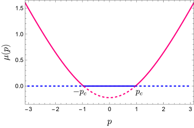
Figure 15: (color online) The solid line, obtained by the maximum of the two largest eigenvalues (80), represents the scgf for the integrated current in the four-state Markov chain in Fig. 14 with parameter value $r=0.2$.

VII A robust mechanism for DPTs

A common feature between the two Markov chain examples in Section. VI is the presence of an absorbing state, from which the system, once entered, can not escape. Their Markov matrices and the associated tilted matrices are reducible making them beyond the purview of the Perron-Forbenius theorem [69]. As a result, crossing of largest eigenvalues is permitted, leading to a singularity in the scgf and, equivalently, a DPT.

This mechanism for DPTs is expected in general for processes with transient states (see illustration in Fig. 16). The transient state space $\mathcal{T}$ is not accessible from the recurrent state space $\mathcal{R}$. Corresponding Markov matrix has the form:

$$\mathbf{M}\equiv\begin{pmatrix}\mathbf{\mathbfcal{T}}&\mathbf{0}\\ \mathbfcal{I}&\mathbf{\mathbfcal{R}}\end{pmatrix},$$ (83)

where $\mathbfcal{T}$ and $\mathbfcal{R}$ are blocks representing transitions within the sub-spaces $\mathcal{T}$ and $\mathcal{R}$, respectively, while $\mathbfcal{I}$ involves transitions from $\mathcal{T}$ to $\mathcal{R}$.

The set of eigenvalues of $\mathbf{M}$ is composed of eigenvalues from $\mathbfcal{T}$ and $\mathbfcal{R}$. At large times, the transient state space $\mathcal{T}$ becomes empty, and the system reaches the stationary state in $\mathcal{R}$. The stationary distribution is given by the eigenvector of $\mathbfcal{R}$ with the largest eigenvalue $e_{1}=1$. This implies that the largest eigenvalue (denoted as $e_{2}$) of $\mathbfcal{T}$ is less than $1$.

For an empirical observable measured in the transient state (as was the case for the examples discussed), only the block $\mathbfcal{T}$ is weighted by the tilting parameter $p$. This means that the spectrum of $\mathbfcal{R}$ remains unchanged with $e_{1}=1$ for all $p$. However, for large $p$, it is expected that the scgf, which is logarithm of the largest eigenvalue of the tilted matrix $\mathbf{M}_{p}$, is positive, implying that $e_{2}>1$ for large $p$. This would occur if $e_{2}$, which was smaller than $e_{1}=1$ for $p=0$, crossed $e_{1}$ at some intermediate value of $p$, resulting in a DPT.

Figure 16: Schematic representation of Markov processes featuring a transient state space $\mathcal{T}$ where the system, once leaving $\mathcal{T}$, cannot reenter from the subspace $\mathcal{R}$.

Remark: The transient states for the examples discussed in this article are explicit. In the example of a drifted Brownian motion, discussed in [48], any finite position is transient as the particle eventually drifts away to infinity.

VIII Multiple phase transitions

Building upon the mechanism of DPT discussed in this article, it is possible to construct simple examples with rich phase behaviours. In the following sections, we explore two such simple examples.

VIII.1 Epidemiological process

Consider a grim epidemiological process where infected individuals quickly die without any chance of recovery. The death rate for an individual is proportional to the number of living persons $n(t)$ at that instant $t$. The scenario is analogous to a variant of Verhulst model [88] of population dynamics with unit reproduction rate. The average number of living persons $\bar{n}(t)$ at a time follows $\frac{d\bar{n}(t)}{dt}\simeq-\alpha\,\bar{n}(t)^{2}$ with $\alpha$ being a parameter, leading to an algebraic decay $\bar{n}(t)\simeq N/(1+\alpha tN)$, where $N$ is the initial size of the population.

A relevant observable is the net resources consumed by the living persons over a period $T$, which is, at the zeroth level approximation and up to a proportionality constant,

$$Q=\int_{0}^{T}n(t)dt.$$ (84)

On an average the consumed resources increase slowly in time $T$ as $\bar{Q}=\alpha^{-1}\log(1+\alpha NT)$ while the fluctuations follow the large deviation asymptotics (2), featuring a piece-wise ldf (see Appendix B for a derivation)

$$\phi(q)=q(2k+1)-k(k+1)\quad\textrm{for {\hbox{k \leq q < k+1}}}$$ (85)

with $k=0,1,\ldots,N-1$. The multiple derivative discontinuities of the ldf are shown in Fig. 17. These discontinuities correspond to first order DPTs between phases characterized by the maximum number of surviving persons $k$ at the time $T$.

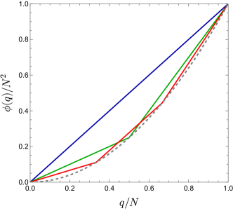
Figure 17: (color online) The ldf (85) for a set of initial population size $N$ (color code: blue $=1$, green $=2$, red $=3$). For large $N$ limit, the scaled ldf $\phi(q)/N^{2}$ converges to the dotted curve $x^{2}$.

VIII.2 Mortal Brownians

A simple extension of the previous example is where the mortal particles diffuse in space. This is a multi-particle generalization of the mortal Brownians introduced in Section. III, where death rate of an individual is proportional to the number of living.

As an observable, we consider the net displacement of all particles

$$Q=\int_{0}^{T}\sum_{i=1}^{N}dx_{i}(t)$$ (86)

where $x_{i}(t)$ is the position of the $i$-th particle at time $t$, and $N$ is the size of the population (living and dead together).

The probability of $Q$ for large time $T$ follows the asymptotics (2) with a piece-wise ldf composed of alternating domains where $\phi(q)$ is linear and quadratic (see Fig. 17). At the boundaries of these domains $\phi^{\prime\prime}(q)$ is discontinuous, indicating a second-order DPT between phases characterized by the number of surviving particles at time $T$. We defer expression of $\phi(q)$ and its derivation in the Appendix C.

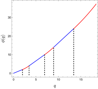
Figure 18: (color online) The ldf $\phi(q)$ for the probability of $Q=qT$ in (86) for three mortal Brownians. Only positive $q$ results are shown. The red color indicates quadratic dependence, while the blue color represents linear dependence.

Remark: The multiple sequence of DPTs in these two examples relate to a transient structure of the state space illustrated in Fig 19. As particles get absorbed, the system moves from one transient state space to the next. A similar sequence of multiple DPTs was recently observed in the context of the occupation fraction of vicious walkers [52].

Figure 19: A Markov process with a sequence of transient state spaces $\mathcal{T}_{i}$ such that evolution can take place only in the direction indicated destined to a recurrent state.

IX Non-Markov processes

The mechanism of DPT that we discussed in Section. VII extends for non-Markovian processes. The key idea is that a non-Markov process with finite memory can be described by a higher dimensional Markov process, which also poses transient sectors if the original process have them. One would expect DPTs for such processes. We give two such examples.

IX.1 Mortal Active Ornstein-Uhlenbeck process

The active Ornstein-Uhlenbeck process [89] is a simple model of persistent dynamics for a non-polar active particle. The position of the particle follows a Langevin dynamics

$$\ddot{X}_{t}+\frac{1}{\tau}\dot{X}_{t}=\eta_{t}$$ (87)

with a Gaussian white noise $\eta_{t}$ with zero-mean and covariance $\langle\eta_{t}\eta_{t^{\prime}}\rangle=2\delta(t-t^{\prime})$. The non-zero auto-correlation $\langle\dot{X}_{t}\dot{X}_{t^{\prime}}\rangle\sim\tau e^{-|t-t^{\prime}|/\tau}$ for large $t-t^{\prime}$ makes the $X_{t}$ dynamics non-Markovian, although on the $(X_{t},\dot{X}_{t})$ space the process is Markovian.

The free propagator for the position of AOUP started at the origin $X_{0}=0$ with $\dot{X}_{0}=0$ is Gaussian:

$$g_{t}(x)=\frac{1}{\sqrt{4\pi t\mathcal{D}_{t}}}\exp\left(-\frac{x^{2}}{4t\mathcal{D}_{t}}\right),$$ (88)

with the variance

$$\mathcal{D}_{t}=\tau^{2}\left(1-\frac{\tau}{2t}\left(3-4e^{-\frac{t}{\tau}}+e^{-\frac{2t}{\tau}}\right)\right).$$ (89)

For a mortal AOUP with a death rate $\alpha$, the probability of the particle position $x$ at time $t$ can be written as (9) with the propagator $g_{t}(x)$ given in (88). For large $t$, the probability has the asymptotic $P_{t}(x=qt)\sim e^{-t\phi(q/\tau)}$ with the ldf that is identical to (10).

This coincidence of the ldf with the Brownian case is not surprising considering that the measurement time $t$ is far larger than the persistance time $\tau$ for the AOUP.

IX.2 Mortal fractional Brownian motion (fBm)

An fBm [90, 91] is a non-Markovian Gaussian process $X_{t}$ with mean zero and power-law auto-correlation:

$$\langle\dot{X}_{t}\dot{X}_{t^{\prime}}\rangle=2H(2H-1)(t-t^{\prime})^{2(H-1)}$$ (90)

for $t>t^{\prime}>0$ with the Hurst exponent $0<H<1$. The free propagator for a fractional Brownian starting at the origin is given by the Gaussian

$$g_{t}(x)=\frac{1}{\sqrt{4\pi t^{2H}}}\exp\left(-\frac{x^{2}}{4t^{2H}}\right).$$ (91)

For a mortal fBm with a death rate $\alpha$, the probability of position at time $t$ is similar to (9) with the propagator in (91). In the limit of large $t$, the probability has the large deviation asymptotic $P_{t}(x=qt^{\nu})\sim e^{-t\phi(q)}$ with the ldf

$$\phi(q)=\begin{dcases}\beta\;|q|^{\frac{1}{\nu}}&\text{for}\ |q|\leq\sqrt{2\alpha/H}\\ \alpha+\frac{q^{2}}{4}&\text{for}\ |q|>\sqrt{2\alpha/H}\end{dcases}$$ (92a)

where $\nu=H+1/2$ and

$$\beta=\frac{\nu\alpha}{H}\left(\frac{H}{2\alpha}\right)^{\frac{1}{2\nu}}.$$ (92b)

Remark: The same ldf was found for an fBm with resetting [27].

X Conclusions

We constructed various illustrative simple models demonstrating DPTs in the statistics of time-integrated observables. These DPTs correspond to sudden changes in effective dynamics that correspond to fluctuations of the observables. For a mathematical origin, we have shown how such DPTs generically arise from the crossing of eigenvalues in reducible Markov operators for stochastic dynamics with transient states. Understanding this scenario aided us in constructing rich phase behaviors consisting of multiple DPTs and extensions for non-Markov processes.

Extending this work for interacting many-body systems and their higher-dimensional generalizations presents intriguing possibilities. For instance, one could explore microscopic models of the epidemiological process in Section. VIII.1 and population dynamics [92, 93], where the density-dependent mortality rate emerges from interactions. Another avenue for investigation could involve studying fluctuations of empirical observables such as integrated current or entropy production in many-particle dynamics with absorbing states. Relying on the mechanism discussed in this work, it is reasonable to predict DPTs in such many-body generalizations. A well-known example [36] is the dynamical phase transition in the current fluctuations of resetting Brownian particles starting from a domain wall initial state on an infinite line. Similar transitions are anticipated for the many-particle generalization of mortal Brownian particles. For such extended systems, the framework of fluctuating hydrodynamics of conditioned dynamics [94] would provide an appropriate theoretical foundation.

In the mechanism discussed here, non-ergodicity arising from the underlying transient state-space is responsible for DPTs. Non-ergodicity may also effectively emerge in the thermodynamic limit of many-body systems or in the low-noise limit of single-degrees of freedom. Exploring the nature and universality of DPTs in such non-ergodic dynamics warrants further investigation.

It is worth noting that that non-ergodicity is not a necessary criteria for DPTs. Singular ldfs are also observed in position distributions in run-and-tumble dynamics devoid of transient states. These singularities originate from a competition between trajectories with typical jumps and trajectories with a dominant atypical jump [38, 37]. Generalization of DPTs in such democratic versus winner-takes-all scenarios would be an interesting future direction.

Appendices

A Boundary condition for absorbing wall

Figure 20: (color online) A continuous time random walker on a 4-site lattice with jump rate $1$, where the site $0$ is absorbing, the site $3$ is reflecting, and the site $2$ (shaded in blue) is where residence time is measured.

The Brownian motion with an absorbing wall studied in Section. V.1 can be viewed as a continuous limit of a continuous-time random walk on a lattice with an absorbing site at $i=0$ and a reflecting wall at the rightmost site. The issue regarding the absorbing boundary condition can be understood already on a four-site problem, illustrated in Fig. 20.

The observable of interest is the residence time at the site $i=2$, defined by $Q=\sum_{1}^{T}\delta_{C_{t},2}$. The corresponding scgf is the largest eigenvalue of the tilted matrix

$$\begin{pmatrix}0&1&0&0\\ 0&-2&1&0\\ 0&1&p-2&1\\ 0&0&1&-1\end{pmatrix}.$$ (93)

which is constructed following the discussion in the Appendix B of [61]. A left eigenvector $(y_{0},y_{1},y_{2},y_{3})$ for the eigenvalue $\lambda$ follows the equation

$$\begin{pmatrix}0\\ y_{0}-2y_{1}+y_{2}\\ y_{1}-2y_{2}+y_{3}+py_{2}\\ y_{2}-y_{3}\end{pmatrix}=\lambda\begin{pmatrix}y_{0}\\ y_{1}\\ y_{2}\\ y_{3}\end{pmatrix},$$ (94)

where the matrices have been transposed for the sake of legibility. We see from $\lambda y_{0}=0$, that a non-zero eigenvalue demands $y_{0}=0$, which in the continuous limit corresponds to the absorbing boundary condition in Sec V.1.2. For the eigenvalue $\lambda=0$, the solution of (94) does not impose vanishing boundary condition at the absorbing site.

In a suitable continuous limit, both eigenvectors satisfy reflecting boundary condition at the rightmost end.

B Large deviation for the epidemiological process

In this section we present a derivation of (85). The probability of $Q$ in (84) with an initial $N$ number of people,

$$P(Q)=\sum_{k=0}^{N}P(Q,k),$$ (95)

where $P(Q,k)$ is the joint probability of $Q$ and that $k$ number of individuals survived till time $T$.

For evaluating this joint probability, consider a sequence of individual deaths at times $t_{1},t_{2},\ldots,t_{N-k}$ in an increasing order of time in the interval $[0,T]$ (see Fig. 21).

Figure 21: A sequence of deaths at times $t_{1},\ldots,t_{N-k}$, with the number of living individuals indicated above the time-line.

In the interval $(t_{i},t_{i+1})$, there are $(N-i)$ living persons, who contribute an amount $(N-i)(t_{i+1}-t_{i})$ to the observable (84). The death rate in this interval is $(N-i)$ and as a result the probability for all of them to survive in this interval and precisely one of them to die in the infinitesimal interval between $t_{i+1}$ and $t_{i+1}+dt_{i+1}$ is $\exp\{-(N-i)^{2}(t_{i+1}-t_{i})\}(N-i)^{2}dt_{i+1}$. Considering all intervals, we write

$$\begin{split}P(Q,k)\sim&\int_{0}^{T}\mathbf{dt}\exp\left(-\sum_{i=0}^{N-k}(N-i)^{2}(t_{i+1}-t_{i})\right)\\ &\qquad\delta\left(Q-\sum_{i=0}^{N-k}(N-i)(t_{i+1}-t_{i})\right),\end{split}$$ (96)

with $\mathbf{dt}=\prod_{i=1}^{N-k}dt_{i}$ subject to the constraint $t_{i}\leq t_{i+1}$, $t_{0}=0$, and $t_{N-k+1}=T$, where we ignored algebraic pre-factors which are irrelevant for large deviation asymptotic.

For our analysis it is convenient to make a change of variables $t_{i}=T\,r_{N+1-i}$, and rewrite (96) as

$$\begin{split}P(qT,k)\sim&\int_{0}^{1}dr_{k+1}\cdots dr_{N}\exp\left(-T\sum_{i=k}^{N}i^{2}(r_{i}-r_{i+1})\right)\\ &\qquad\delta\left(\sum_{i=k}^{N}i(r_{i}-r_{i+1})-q\right),\end{split}$$ (97)

with $r_{k}=1$, $r_{N+1}=0$, and $r_{i}\geq r_{i+1}$.

Evidently, for large $T$, the integral in (97) is dominated by the minimum of the term in the exponential subjected to the constraint in the delta function. This gives the large deviation asymptotic $P(qT,k)\sim e^{-T\phi_{k}(q)}$ with

$$\phi_{k}(q)=\min_{\{r_{i}\}}\sum_{i=k}^{N}i^{2}(r_{i}-r_{i+1})$$ (98)

subjected to constraint $\sum_{i=k}^{N}i(r_{i}-r_{i+1})=q$.

To solve this variational problem, we rewrite (98) using $r_{1}=1$ and $r_{N+1}=0$, resulting in

$$\phi(q)=\min_{\{r_{i}\}}\sum_{i=k+1}^{N}(2i-1)r_{i}+k^{2}$$ (99)

with constraint $\sum_{i=k+1}^{N}r_{i}+k=q$. Considering that each term in the summation in (99) is positive, minimum is achieved by setting as many $r_{i}=0$ as possible. The domain of integration $r_{i}\geq r_{i+1}$ imposes that for a minimal solution $r_{i}=0$ for all $i\geq i^{\star}$ dictated by the value of $q$ in the constraint $\sum_{i=k+1}^{i^{\star}-1}r_{i}+k=q$.

Evidently, for $q<k$ and $q>N$, the constraint can not be satisfied, implying $P(qT,k)=0$ and consequently $\phi_{k}(q)\to\infty$. For $k\leq q<k+1$, minimum solution corresponds to $i^{\star}=k+2$ and $r_{k+1}=q-k$. Similarly, for $k+1\leq q<k+2$, the minimum corresponds to $i^{\star}=k+3$, $r_{k+1}=1$, $r_{k+2}=q-k-1$, and $r_{i}=0$ for the rest; and so on. This gives the solution of the variational problem

$$\phi_{k}(q)=\{2(k+n)+1\}q-(k+n)(k+n+1)$$ (100)

for $k+n\leq q<k+n+1$ with $n=0,\cdots,N-k-1$.

Using this asymptotic of $P(Q,k)$ in (95) yields the large deviation asymptotic (2) for $P(Q)$ with $\phi(q)=\min\{\phi_{0}(q),\ldots,\phi_{N}(q)\}$ leading to the expression (85).

C Large deviation for the mortal Brownians

Here, we present a derivation for the piece-wise large deviation function discussed in Section. VIII.2. For this problem, the joint probability (analogous to (96)) is

$$\begin{split}P(Q,k)\sim\int_{0}^{T}\mathbf{dt}&\exp\left(-\sum_{i=0}^{N-k}(N-i)^{2}(t_{i+1}-t_{i})\right)\\ \int\limits_{-\infty}^{\infty}\mathbf{dx}&\exp\left(-\sum_{i=1}^{N}\frac{x_{i}^{2}}{4t_{i}}\right)\delta\left(Q-\sum_{i=0}^{N}x_{i}\right)\end{split}$$

with $t_{i}=T$ for $i>N-k$, $\mathbf{dt}=dt_{1}\ldots dt_{N}$ and $\mathbf{dx}\equiv dx_{1}\ldots dx_{N}$, where we have used the Gaussian propagator for Brownains of unit diffusivity. At this point onward the analysis is similar to the one discussed in Appendix. B. For brevity, we present the final expression of the large deviation function.

The probability of $Q$ for large time $T$ follows the asymptotics (2) with a piece-wise ldf

$$\phi(q)=\begin{dcases}\frac{q^{2}}{4k}+k^{2}&\textrm{for }\ell_{k-1}\leq|q|\leq\frac{k\ell_{k}}{k+1}\cr|q|\sqrt{2k+1}-k(k+1)&\textrm{for }\frac{k\ell_{k}}{k+1}\leq|q|\leq\ell_{k},\end{dcases}$$ (101)

where $k=0,1,\ldots,N$, $\ell_{k}=2(k+1)\sqrt{2k+1}$ for all $k<N$, and $\ell_{N}$ infinite.

D Expressions of quantities defined in Section. IV.1

The solutions $S_{s}$ and $F_{s}$ for the local time observable are obtained by solving (37b) and (38b), and are given by (39), with the explicit expressions

$$n_{1}(u,p,x_{0})=\begin{dcases}\frac{1}{u^{2}}\left(d(u,p)-2p\sinh\left(\frac{au}{2}\right)\cosh\left(u(L-a)\right)\cosh\left(\frac{1}{2}u(a-2x_{0})\right)-u\cosh\left(u(x_{0}-L)\right)\right)&x_{0}\leq a,\\ \frac{1}{u^{2}}\left(d(u,p)-\left(p\sinh\left(au\right)+u\right)\cosh\left(u(x_{0}-L)\right)\right)&x_{0}>a,\end{dcases}$$

$$n_{2}(u,p,x_{0})=\begin{dcases}u\cosh\left(u(x_{0}-L)\right)-p\cosh\left(u(a-L)\right)\sinh\left(u(x_{0}-a)\right)&x_{0}\leq a,\\ u\cosh\left(u(x_{0}-L)\right)&x_{0}>a,\end{dcases}$$

and $d(u,p)$ defined in (40).

References

- Baek and Kafri [2015] Y. Baek and Y. Kafri, Singularities in large deviation functions, Journal of Statistical Mechanics: Theory and Experiment 2015, P08026 (2015).
- Baek et al. [2017] Y. Baek, Y. Kafri, and V. Lecomte, Dynamical symmetry breaking and phase transitions in driven diffusive systems, Physical review letters 118, 030604 (2017).
- Bertini et al. [2010] L. Bertini, A. De Sole, D. Gabrielli, G. Jona-Lasinio, and C. Landim, Lagrangian phase transitions in nonequilibrium thermodynamic systems, Journal of Statistical Mechanics: Theory and Experiment 2010, L11001 (2010).
- Bunin et al. [2013] G. Bunin, Y. Kafri, and D. Podolsky, Cusp singularities in boundary-driven diffusive systems, Journal of Statistical Physics 152, 112 (2013).
- Aminov et al. [2014] A. Aminov, G. Bunin, and Y. Kafri, Singularities in large deviation functionals of bulk-driven transport models, Journal of Statistical Mechanics: Theory and Experiment 2014, P08017 (2014).
- Shpielberg et al. [2017] O. Shpielberg, Y. Don, and E. Akkermans, Numerical study of continuous and discontinuous dynamical phase transitions for boundary-driven systems, Physical Review E 95, 032137 (2017).
- Kumar et al. [2011] N. Kumar, S. Ramaswamy, and A. Sood, Symmetry properties of the large-deviation function of the velocity of a self-propelled polar particle, Physical review letters 106, 118001 (2011).
- Bodineau and Derrida [2005] T. Bodineau and B. Derrida, Distribution of current in nonequilibrium diffusive systems and phase transitions, Physical Review E 72, 066110 (2005).
- Bertini et al. [2005] L. Bertini, A. De Sole, D. Gabrielli, G. Jona-Lasinio, and C. Landim, Current fluctuations in stochastic lattice gases, Physical review letters 94, 030601 (2005).
- Bertini et al. [2006] L. Bertini, A. D. Sole, D. Gabrielli, G. Jona-Lasinio, and C. Landim, Non equilibrium current fluctuations in stochastic lattice gases, Journal of statistical physics 123, 237 (2006).
- Garrahan et al. [2007] J. P. Garrahan, R. L. Jack, V. Lecomte, E. Pitard, K. van Duijvendijk, and F. van Wijland, Dynamical first-order phase transition in kinetically constrained models of glasses, Physical review letters 98, 195702 (2007).
- Garrahan et al. [2009] J. P. Garrahan, R. L. Jack, V. Lecomte, E. Pitard, K. van Duijvendijk, and F. van Wijland, First-order dynamical phase transition in models of glasses: an approach based on ensembles of histories, Journal of Physics A: Mathematical and Theoretical 42, 075007 (2009).
- Le Doussal et al. [2016] P. Le Doussal, S. N. Majumdar, and G. Schehr, Large deviations for the height in 1d kardar-parisi-zhang growth at late times, EPL (Europhysics Letters) 113, 60004 (2016).
- Janas et al. [2016] M. Janas, A. Kamenev, and B. Meerson, Dynamical phase transition in large-deviation statistics of the kardar-parisi-zhang equation, Physical Review E 94, 032133 (2016).
- Cagnetta et al. [2017] F. Cagnetta, F. Corberi, G. Gonnella, and A. Suma, Large fluctuations and dynamic phase transition in a system of self-propelled particles, Physical review letters 119, 158002 (2017).
- Nemoto et al. [2019] T. Nemoto, É. Fodor, M. E. Cates, R. L. Jack, and J. Tailleur, Optimizing active work: Dynamical phase transitions, collective motion, and jamming, Physical Review E 99, 022605 (2019).
- Coghi et al. [2019] F. Coghi, J. Morand, and H. Touchette, Large deviations of random walks on random graphs, Physical Review E 99, 022137 (2019).
- Szavits-Nossan et al. [2014] J. Szavits-Nossan, M. R. Evans, and S. N. Majumdar, Constraint-driven condensation in large fluctuations of linear statistics, Physical review letters 112, 020602 (2014).
- Jack and Sollich [2013] R. L. Jack and P. Sollich, Large deviations of the dynamical activity in the east model: Analysing structure in biased trajectories, Journal of Physics A: Mathematical and Theoretical 47, 015003 (2013).
- Bodineau and Derrida [2007] T. Bodineau and B. Derrida, Cumulants and large deviations of the current through non-equilibrium steady states, Comptes Rendus Physique 8, 540 (2007).
- Prolhac and Mallick [2009] S. Prolhac and K. Mallick, Cumulants of the current in a weakly asymmetric exclusion process, Journal of Physics A: Mathematical and Theoretical 42, 175001 (2009).
- Hurtado and Garrido [2011] P. I. Hurtado and P. L. Garrido, Spontaneous symmetry breaking at the fluctuating level, Physical review letters 107, 180601 (2011).
- Shpielberg et al. [2018] O. Shpielberg, T. Nemoto, and J. Caetano, Universality in dynamical phase transitions of diffusive systems, Physical Review E 98, 052116 (2018).
- Bodineau et al. [2012] T. Bodineau, V. Lecomte, and C. Toninelli, Finite size scaling of the dynamical free-energy in a kinetically constrained model, Journal of Statistical Physics 147, 1 (2012).
- Speck et al. [2012] T. Speck, A. Engel, and U. Seifert, The large deviation function for entropy production: the optimal trajectory and the role of fluctuations, Journal of Statistical Mechanics: Theory and Experiment 2012, P12001 (2012).
- Nyawo and Touchette [2016] P. T. Nyawo and H. Touchette, Large deviations of the current for driven periodic diffusions, Physical Review E 94, 032101 (2016).
- Majumdar et al. [2015a] S. N. Majumdar, S. Sabhapandit, and G. Schehr, Dynamical transition in the temporal relaxation of stochastic processes under resetting, Physical Review E 91, 052131 (2015a).
- Pal et al. [2016] A. Pal, A. Kundu, and M. R. Evans, Diffusion under time-dependent resetting, Journal of Physics A: Mathematical and Theoretical 49, 225001 (2016).
- Harris and Touchette [2017] R. J. Harris and H. Touchette, Phase transitions in large deviations of reset processes, Journal of Physics A: Mathematical and Theoretical 50, 10LT01 (2017).
- Majumdar et al. [2015b] S. N. Majumdar, S. Sabhapandit, and G. Schehr, Random walk with random resetting to the maximum position, Physical Review E 92, 052126 (2015b).
- Santra et al. [2022] I. Santra, U. Basu, and S. Sabhapandit, Effect of stochastic resetting on brownian motion with stochastic diffusion coefficient, Journal of Physics A: Mathematical and Theoretical 55, 414002 (2022).
- Smith and Majumdar [2022] N. R. Smith and S. N. Majumdar, Condensation transition in large deviations of self-similar gaussian processes with stochastic resetting, Journal of Statistical Mechanics: Theory and Experiment 2022, 053212 (2022).
- Biroli et al. [2023] M. Biroli, H. Larralde, S. N. Majumdar, and G. Schehr, Extreme statistics and spacing distribution in a brownian gas correlated by resetting, Physical Review Letters 130, 207101 (2023).
- Gupta [2019] D. Gupta, Stochastic resetting in underdamped brownian motion, Journal of Statistical Mechanics: Theory and Experiment 2019, 033212 (2019).
- Gupta et al. [2020] D. Gupta, C. A. Plata, A. Kundu, and A. Pal, Stochastic resetting with stochastic returns using external trap, Journal of Physics A: Mathematical and Theoretical 54, 025003 (2020).
- Di Bello et al. [2023] C. Di Bello, A. K. Hartmann, S. N. Majumdar, F. Mori, A. Rosso, and G. Schehr, Current fluctuations in stochastically resetting particle systems, Physical Review E 108, 014112 (2023).
- Mori et al. [2021a] F. Mori, P. Le Doussal, S. N. Majumdar, and G. Schehr, Condensation transition in the late-time position of a run-and-tumble particle, Physical Review E 103, 062134 (2021a).
- Mori et al. [2021b] F. Mori, G. Gradenigo, and S. N. Majumdar, First-order condensation transition in the position distribution of a run-and-tumble particle in one dimension, Journal of Statistical Mechanics: Theory and Experiment 2021, 103208 (2021b).
- Gradenigo and Majumdar [2019] G. Gradenigo and S. N. Majumdar, A first-order dynamical transition in the displacement distribution of a driven run-and-tumble particle, Journal of Statistical Mechanics: Theory and Experiment 2019, 053206 (2019).
- Mallmin et al. [2019] E. Mallmin, R. A. Blythe, and M. R. Evans, A comparison of dynamical fluctuations of biased diffusion and run-and-tumble dynamics in one dimension, Journal of Physics A: Mathematical and Theoretical 52, 425002 (2019).
- Santra et al. [2020] I. Santra, U. Basu, and S. Sabhapandit, Run-and-tumble particles in two dimensions under stochastic resetting conditions, Journal of Statistical Mechanics: Theory and Experiment 2020, 113206 (2020).
- Proesmans et al. [2020] K. Proesmans, R. Toral, and C. Van den Broeck, Phase transitions in persistent and run-and-tumble walks, Physica A: Statistical Mechanics and its Applications 552, 121934 (2020).
- Banerjee et al. [2020] T. Banerjee, S. N. Majumdar, A. Rosso, and G. Schehr, Current fluctuations in noninteracting run-and-tumble particles in one dimension, Physical Review E 101, 052101 (2020).
- Mukherjee et al. [2024] S. Mukherjee, P. Le Doussal, and N. R. Smith, Large deviations in statistics of the local time and occupation time for a run and tumble particle, Physical Review E 110, 024107 (2024).
- Smith and Meerson [2019] N. R. Smith and B. Meerson, Geometrical optics of constrained brownian excursion: from the kpz scaling to dynamical phase transitions, Journal of Statistical Mechanics: Theory and Experiment 2019, 023205 (2019).
- Meerson and Smith [2019] B. Meerson and N. R. Smith, Geometrical optics of constrained brownian motion: three short stories, Journal of Physics A: Mathematical and Theoretical 52, 415001 (2019).
- Nyawo and Touchette [2017] P. T. Nyawo and H. Touchette, A minimal model of dynamical phase transition, Europhysics Letters 116, 50009 (2017).
- Nyawo and Touchette [2018] P. T. Nyawo and H. Touchette, Dynamical phase transition in drifted brownian motion, Physical Review E 98, 052103 (2018).
- Majumdar and Meerson [2020a] S. N. Majumdar and B. Meerson, Statistics of first-passage brownian functionals, Journal of Statistical Mechanics: Theory and Experiment 2020, 023202 (2020a).
- Whitelam and Jacobson [2021] S. Whitelam and D. Jacobson, Varied phenomenology of models displaying dynamical large-deviation singularities, Physical Review E 103, 032152 (2021).
- Gingrich et al. [2014] T. R. Gingrich, S. Vaikuntanathan, and P. L. Geissler, Heterogeneity-induced large deviations in activity and (in some cases) entropy production, Physical Review E 90, 042123 (2014).
- Mukherjee and Smith [2023] S. Mukherjee and N. R. Smith, Dynamical phase transition in the occupation fraction statistics for noncrossing brownian particles, Physical Review E 107, 064133 (2023).
- Majumdar and Meerson [2020b] S. N. Majumdar and B. Meerson, Toward the full short-time statistics of an active brownian particle on the plane, Physical Review E 102, 022113 (2020b).
- Szavits-Nossan and Evans [2015] J. Szavits-Nossan and M. R. Evans, Inequivalence of nonequilibrium path ensembles: the example of stochastic bridges, Journal of Statistical Mechanics: Theory and Experiment 2015, P12008 (2015).
- Kanazawa et al. [2024a] T. Kanazawa, K. Kawaguchi, and K. Adachi, Dynamical phase transitions in single particle brownian motion without drift, arXiv preprint arXiv:2407.18282 (2024a).
- Kanazawa et al. [2024b] T. Kanazawa, K. Kawaguchi, and K. Adachi, Universality in the dynamical phase transitions of brownian motion, arXiv preprint arXiv:2407.14090 (2024b).
- Jack and Sollich [2010] R. L. Jack and P. Sollich, Large deviations and ensembles of trajectories in stochastic models, Progress of Theoretical Physics Supplement 184, 304 (2010).
- Jack and Sollich [2015] R. L. Jack and P. Sollich, Effective interactions and large deviations in stochastic processes, The European Physical Journal Special Topics 224, 2351 (2015).
- Chetrite and Touchette [2013] R. Chetrite and H. Touchette, Nonequilibrium microcanonical and canonical ensembles and their equivalence, Physical review letters 111, 120601 (2013).
- Chetrite and Touchette [2015] R. Chetrite and H. Touchette, Nonequilibrium markov processes conditioned on large deviations, Annales Henri Poincaré 16, 2005 (2015).
- Derrida and Sadhu [2019a] B. Derrida and T. Sadhu, Large deviations conditioned on large deviations i: Markov chain and langevin equation, Journal of Statistical Physics 176, 773 (2019a).
- Majumdar [2005] S. N. Majumdar, Brownian functionals in physics and computer science, Current Science 89, 2076 (2005).
- Majumdar and Orland [2015] S. N. Majumdar and H. Orland, Effective langevin equations for constrained stochastic processes, Journal of Statistical Mechanics: Theory and Experiment 2015, P06039 (2015).
- De Bruyne et al. [2021a] B. De Bruyne, S. N. Majumdar, and G. Schehr, Generating constrained run-and-tumble trajectories, Journal of Physics A: Mathematical and Theoretical 54, 385004 (2021a).
- De Bruyne et al. [2021b] B. De Bruyne, S. N. Majumdar, H. Orland, and G. Schehr, Generating stochastic trajectories with global dynamical constraints, Journal of Statistical Mechanics: Theory and Experiment 2021, 123204 (2021b).
- Grela et al. [2021] J. Grela, S. N. Majumdar, and G. Schehr, Non-intersecting Brownian Bridges in the Flat-to-Flat Geometry, Journal of Statistical Physics 183, 49 (2021).
- Goldenfeld [1992] N. Goldenfeld, Lectures on phase transitions and the renormalization group, Westview Press (1992).
- Dhar [2011] D. Dhar, Graphical Enumeration Techniques: Series Expansions and Animal Problems, in Computational Statistical Physics (Hindustan Book Agency, 2011) pp. 35–54.
- Cuesta and Sánchez [2004] J. A. Cuesta and A. Sánchez, General non-existence theorem for phase transitions in one-dimensional systems with short range interactions, and physical examples of such transitions, Journal of statistical physics 115, 869 (2004).
- Touchette [2009] H. Touchette, The large deviation approach to statistical mechanics, Physics Reports 478, 1 (2009).
- Majumdar and Schehr [2017] S. N. Majumdar and G. Schehr, Large deviations (2017), arXiv:1711.07571 [cond-mat.stat-mech] .
- Mazzolo and Monthus [2022] A. Mazzolo and C. Monthus, Conditioning diffusion processes with killing rates, Journal of Statistical Mechanics: Theory and Experiment 2022, 083207 (2022).
- Berman and Halina [1996] S. M. Berman and F. Halina, Distributions associated with markov processes with killing, Stochastic Models 12, 367 (1996).
- Holcman et al. [2005] D. Holcman, A. Marchewka, and Z. Schuss, The survival probability of diffusion with killing, arXiv preprint math-ph/0502035 (2005).
- Frydman [2000] H. Frydman, Gussian diffusions and continuous state branching processes with killing, Stochastic Models 16, 189 (2000).
- Chen et al. [2022] Y. Chen, T. T. Georgiou, and M. Pavon, The most likely evolution of diffusing and vanishing particles: Schrodinger bridges with unbalanced marginals, SIAM Journal on Control and Optimization 60, 2016 (2022).
- Hartmann [2015] A. K. Hartmann, Big practical guide to computer simulations, World Scientific Publishing Company (2015).
- Hartmann et al. [2023] A. K. Hartmann, S. N. Majumdar, and G. Schehr, The distribution of the maximum of independent resetting brownian motions, arXiv preprint arXiv:2309.17432 (2023).
- Nickelsen and Touchette [2018] D. Nickelsen and H. Touchette, Anomalous Scaling of Dynamical Large Deviations, Physical Review Letters 121, 090602 (2018).
- Krapivsky et al. [2014] P. Krapivsky, K. Mallick, and T. Sadhu, Melting of an ising quadrant, Journal of Physics A: Mathematical and Theoretical 48, 015005 (2014).
- Pal et al. [2019] A. Pal, R. Chatterjee, S. Reuveni, and A. Kundu, Local time of diffusion with stochastic resetting, Journal of Physics A: Mathematical and Theoretical 52, 264002 (2019).
- Burenev et al. [2023a] I. N. Burenev, S. N. Majumdar, and A. Rosso, Local time of a system of brownian particles on the line with steplike initial condition, Physical Review E 108, 064113 (2023a).
- Burenev et al. [2023b] I. N. Burenev, S. N. Majumdar, and A. Rosso, Occupation time of a system of brownian particles on the line with steplike initial condition, arXiv preprint arXiv:2311.17689 (2023b).
- [84] Supplemental mathematica notebook containing explicit solutions, and , for the residence time of a Brownian motion confined within an absorbing wall and a reflecting wall.
- Monthus and Mazzolo [2022] C. Monthus and A. Mazzolo, Conditioned diffusion processes with an absorbing boundary condition for finite or infinite horizon, Phys. Rev. E 106, 044117 (2022).
- du Buisson and Touchette [2020] J. du Buisson and H. Touchette, Dynamical large deviations of reflected diffusions, Physical Review E 102, 012148 (2020).
- Kittel [1969] C. Kittel, Phase transition of a molecular zipper, American Journal of Physics 37, 917 (1969).
- Meerson and Ovaskainen [2013] B. Meerson and O. Ovaskainen, Immigration-extinction dynamics of stochastic populations, Phys. Rev. E 88, 012124 (2013).
- Martin et al. [2021] D. Martin, J. O’Byrne, M. E. Cates, É. Fodor, C. Nardini, J. Tailleur, and F. Van Wijland, Statistical mechanics of active ornstein-uhlenbeck particles, Physical Review E 103, 032607 (2021).
- Sadhu and Wiese [2021] T. Sadhu and K. J. Wiese, Functionals of fractional brownian motion and the three arcsine laws, Physical Review E 104, 054112 (2021).
- Sadhu et al. [2018] T. Sadhu, M. Delorme, and K. J. Wiese, Generalized arcsine laws for fractional brownian motion, Physical review letters 120, 040603 (2018).
- Ovaskainen and Meerson [2010] O. Ovaskainen and B. Meerson, Stochastic models of population extinction, Trends in Ecology I& Evolution 25, 643 (2010).
- Ottino-Löffler and Kardar [2020] B. Ottino-Löffler and M. Kardar, Population extinction on a random fitness seascape, Phys. Rev. E 102, 052106 (2020).
- Derrida and Sadhu [2019b] B. Derrida and T. Sadhu, Large Deviations Conditioned on Large Deviations II: Fluctuating Hydrodynamics, J. Stat. Phys. 177, 151 (2019b).
- Baek et al. [2018] Y. Baek, Y. Kafri, and V. Lecomte, Dynamical phase transitions in the current distribution of driven diffusive channels, Journal of Physics A: Mathematical and Theoretical 51, 105001 (2018).