Hybrid Local Causal Discovery

Abstract

Local causal discovery aims to learn and distinguish the direct causes and effects of a target variable from observed data. Existing constraint-based local causal discovery methods use AND or OR rules in constructing the local causal skeleton, but using either rule alone is prone to produce cascading errors in the learned local causal skeleton, and thus impacting the inference of local causal relationships. On the other hand, directly applying score-based global causal discovery methods to local causal discovery may randomly return incorrect results due to the existence of local equivalence classes. To address the above issues, we propose a Hybrid Local Causal Discovery algorithm, called HLCD. Specifically, HLCD initially utilizes a constraint-based approach combined with the OR rule to obtain a candidate skeleton and then employs a score-based method to eliminate redundant portions in the candidate skeleton. Furthermore, during the local causal orientation phase, HLCD distinguishes between V-structures and equivalence classes by comparing the local structure scores between the two, thereby avoiding orientation interference caused by local equivalence classes. We conducted extensive experiments with seven state-of-the-art competitors on 14 benchmark Bayesian network datasets, and the experimental results demonstrate that HLCD significantly outperforms existing local causal discovery algorithms.

1 Introduction

Causal discovery has always been an important goal in many areas of scientific research [1, 2]. It reveals the underlying causal mechanisms of data generation and contributes to solving decision-making problems in machine learning  [3, 4]. Learning a Bayesian network (BN) from observational data is the popular method for causal discovery [5, 6]. The structure of a BN takes the form of a directed acyclic graph (DAG), where nodes signify variables, and edges represent cause-effect relationships between variables [7]. In recent years, many global causal discovery algorithms have been proposed, which aim to learn the entire causal network of all variables, such as MMHC [8], GGSL [9], and ADL [10]. However, in many practical scenarios, it is not necessary to waste time learning a global causal network when we are only interested in the causal relationships around a given variable [11]. To address this challenge, local causal discovery algorithms have been proposed.

Local causal discovery aims to uncover the causal structure surrounding a specific variable. However, due to the unavailability of complete global information, many edge directions determined by relationships with distant variables remain unidentified. As a result, most existing methods adopt a progressive learning approach to gradually acquire outer layer information, until the causal directions around the target variable are identified. Consequently, local causal discovery commonly employs the faster constraint-based methods [12, 13], as score-based methods exhibit higher time complexity and are not well-suited for this gradual information acquisition process [14].

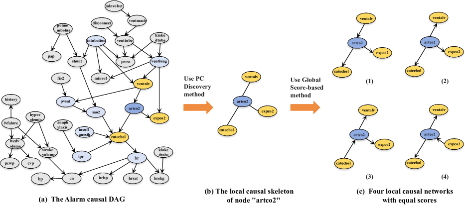
Figure 1: Directly using the search scoring algorithm to find the maximum score local network structure of node “artco2” will randomly return one of the four local structures in (c). It may depend on the order in which the variables in the dataset are encountered.

Similar to global causal discovery methods, local causal discovery is susceptible to common issues associated with conditional independence (CI) testing [15], which can impact its accuracy [16, 17]. One prominent concern is that CI testing cannot accurately determine the causal skeleton. As a result, many approaches employ symmetry tests to address this limitation. However, the prevailing AND and OR rules used in these tests introduce certain errors [18, 19]. The AND rule aims to rigorously eliminate all erroneous relationships, while the OR rule [19] seeks to include as many true positives as possible, operating under a more lenient criterion. Empirical studies have provided evidence that approaches based on the AND rule achieve superior precision, whereas methods based on the OR rule exhibit better performance in terms of recall [20]. Consequently, neither approach yields completely accurate results. Additionally, in the context of local causal learning, the presence of data bias caused by unconsidered distant relationships and inherent noise in the data further compounds the negative impact, exacerbating the potential for misleading results in local causal discovery.

To address the challenges posed by the dual absence of sample and global information, a natural approach is to leverage a hybrid methodology for local causal structure discovery, aiming to enhance performance by combining the strengths of constraint-based and score-based methods. While hybrid methods are commonly employed in global causal discovery research, their application in local causal discovery remains relatively unexplored. The complexity arises because a straightforward combination of these two methods inevitably faces the efficiency dilemma mentioned earlier in score-based approaches. Moreover, directly utilizing a global search scoring method to find the maximum score of local network structures may lead to incorrect local causal networks due to local equivalence class issues, as shown in Fig. 1. Furthermore, inaccuracies in CI tests resulting from information miss cascade into errors in the score-based causal discovery process. Consequently, effectively leveraging score information in local causal discovery poses a significant challenge.

In this paper, we introduce a novel hybrid method that identifies causal skeletons and V-structures by comparing scores among different local causal structures. Specifically, we employ the constraint-based approach for the initial causal skeleton, which uses symmetric tests with the OR rule to achieve a comprehensive yet less precise network. On this basis, we demonstrate the identification and removal of redundant structures through special local structures between the target variable and its causes and effects. Additionally, we prove the discovery of V-structures using similar score information. This theoretical contribution motivates us to propose a novel hybrid local causal discovery method. Our main contributions are summarized as follows:

• We theoretically analyze the special local structure score relationships between the target variable and its causal variables, as well as different local structure score relationships between equivalence classes and V-structures.

• We propose a Hybrid Local Causal Discovery algorithm, HLCD. Based on our analysis, HLCD can effectively eliminate redundant causal skeletons and differentiate between V-structures and equivalence classes by scoring to avoid interference caused by score equivalence.

• We conducted extensive experiments using seven state-of-the-art local causal discovery algorithms on 14 benchmark BN datasets. The results show that our proposed algorithms outperform the compared methods, especially in the small sample case.

The remainder of this paper is organized as follows. Section 2 reviews the related work and Section 3 gives the notations and definitions. Section 4 describes the proposed HLCD algorithm in detail and Section 5 reports the experimental results. Section 6 summarizes the paper.

2 Relate Work

The majority of local causal discovery algorithms are constraint-based. They both use CI tests singularly to construct and orient causal networks. Some pioneering algorithms, Local Causal Discovery (LCD) [21] and its variants, use CI tests to learn the causal relationships among every four variables. BLCD learns the Y-structure in the MB of a target variable [22]. While LCD/BLCD algorithms aim to identify a subset of causal edges via special structures among all variables, not distinguishing between the direct causes and effects of the target.

To address this problem, state-of-the-art local causal discovery algorithms distinguish the direct causes and effects of the target variable directly in the observed data. PCD-by-PCD [23] uses the MMPC to find PC, separating sets, and AND rule for local skeleton construction and V-structure identification. Then, the found V-structures and Meek-rules [24] are used to achieve edge orientations. MB-by-MB [25] first finds a MB of the target node and constructs a local causal structure, and then sequentially finds MB of variables connected to the target and simultaneously constructs local structures along the paths starting from the target until the causes and effects of the target have been determined. Causal Markov Blanket (CMB) [26], first uses HITON-MB [27] to find the MB of the target, and then orients edges by tracking the conditional independence changes in MBs. LCS-FS [28] uses mutual information-based feature selection methods [29] to discover the PC set of variables and construct the skeleton using OR rules. Unfortunately, it cannot discover the separating sets between nodes while learning the PC sets of nodes. Therefore, LCS-FS looks for separating sets from a subset of the learned PC sets and in turn uses the separating sets for edge orientation. Yang et al. propose the concept of N-structures. Through leveraging the N-structures, ELCS [30] discovers the local structure of the target variable while learning as few MBs of the variable as possible, which reduce the number and impact of unreliable CI tests. PSL [31] is a partial causal discovery algorithm. It uses the OR rule to construct the skeleton and recursively finds two types of v-structures, Type-C and Type-NC, in the PC set of the current node until all edges in the partial BN structure are oriented, avoiding the false edge orientation problem of local causal discovery algorithms. Recently, Yang et al. proposed a gradient-based method for learning local causal structure, GraN-LCS [14] constructs an MLP to simultaneously fit all other variables for a target variable and defines an acyclicity-constrained local recovery loss to promote the exploration of local graphs and to find out direct causes and effects.

However, as we discussed in Section 1, existing local causal discovery algorithms do not consider utilizing score information in the data to enhance the performance of the algorithm when faced with challenges such as sample size, noise, and global information deficiencies. In this paper, we will develop a novel hybrid local discovery algorithm to improve the quality of local causal discovery, especially in the case of small samples.

3 Notations And Definitions

In this section, we will briefly introduce some basic notations and definitions.

Definition 1 (Bayesian Network). [7] Let U denote a set of random variables and $\Theta$ indicate the conditional probability distribution of each node $X\in\textbf{U}$ given its parents. A Bayesian Network, ${\mathbb{B}}(\mathcal{G},\Theta)$, is represented by a tuple consisting of a DAG $\mathcal{G}$, and a set of parameters $\Theta$.

In a BN ${\mathbb{B}}(\mathcal{G},\Theta)$, each variable in $\mathcal{G}$ is independent of any subset of its non-descendants given its parents. We can decompose the joint probability distribution into local conditional probabilities using Markov conditioning.

Definition 2 (V-Structure). [7] The triplet of variables $X$, $Y$, and $T$ forms a V-structure if node $T$ has two incoming edges from $X$ and $Y$ respectively, i.e. $X\rightarrow T\leftarrow Y$, and $X$ is not adjacent to $Y$.

In a BN, $T$ is a collider if two directed edges are from $X$ to $T$ and $Y$ to $T$, respectively. i.e., the cause variables of colliding nodes can be recognized by the V-structure.

Definition 3 (Symmetry Constraint). [32] For a node $X$ to be a parent or child of $Y$ in a DAG. Then, $X$ must be in the PC set of $Y$ and $Y$ must be in the PC set of $X$, i.e., $X\in\textbf{PC}_{Y}$ and $Y\in\textbf{PC}_{X}$.

In a BN, learning causal relationships between variables from data is sometimes asymmetric. In this case, using only the AND or OR rule individually to eliminate causal asymmetry does not lead to accurate results [18].

Definition 4 (Score Consistency). [33] Let $\mathcal{D}$ be a set of data consisting of i.i.d. samples from some distribution ${\mathcal{P}}$. A score criterion $\mathcal{S}$ is consistent if, as the size of the $\mathcal{D}$ goes to infinity, the following two properties hold true:

1. if the structure $\mathcal{G}$ contains ${\mathcal{P}}$ and another structure $\mathcal{G}^{\prime}$ does not, then $\mathcal{S}(\mathcal{G},\mathcal{D})>\mathcal{S}(\mathcal{G}^{\prime},\mathcal{D})$.

2. if $\mathcal{G}$ and $\mathcal{G}^{\prime}$ both contain ${\mathcal{P}}$ but $\mathcal{G}$ has fewer parameters, then $\mathcal{S}(\mathcal{G},\mathcal{D})>\mathcal{S}(\mathcal{G}^{\prime},\mathcal{D})$.

The graph $\mathcal{G}$ contains ${\mathcal{P}}$ if there exists a set of parameter values $\Theta$ for $\mathcal{G}$ such that the parameterized BN model $(\mathcal{G},\Theta)$ represents ${\mathcal{P}}$ exactly.

Definition 5 (Local Score Consistency). [33] Let $\mathcal{D}$ be a set of data consisting of i.i.d. samples from some distribution ${\mathcal{P}}$. Let $\mathcal{G}$ be any BN structure and $\mathcal{G}^{\prime}$ be the same structure as $\mathcal{G}$ but with an edge from a node $Y$ to a node $X$. Let $\textbf{PC}_{X}^{\mathcal{G}}$ be the parent set of $X$ in $\mathcal{G}$. A score criterion $\mathcal{S}$ is locally consistent if, as the size of the $\mathcal{D}$ goes to infinity, the following two properties hold true:

1. if $X\not\!\perp\!\!\!\perp Y\mid\textbf{PC}_{X}^{\mathcal{G}}$, then $\mathcal{S}(\mathcal{G},\mathcal{D})<\mathcal{S}(\mathcal{G}^{\prime},\mathcal{D})$.

2. if $X\!\perp\!\!\!\perp Y\mid\textbf{PC}_{X}^{\mathcal{G}}$, then $\mathcal{S}(\mathcal{G},\mathcal{D})>\mathcal{S}(\mathcal{G}^{\prime},\mathcal{D})$.

The score-based methods rely on score criteria to learn the best-fit DAG $\mathcal{G}$ for the data samples. In general, the higher the score for $\mathcal{G}$, the better the fit to the data $\mathcal{D}$, and vice versa.

For example, information theoretic scores [34] aim to avoid over-fitting by balancing the goodness of fit with model dimensionality given the available data. The general form of these scores can be expressed as:

$$\mathcal{S}(\mathcal{G},\mathcal{D})=\log[\hat{p}(\mathcal{D}|\mathcal{G})]-\Delta(\mathcal{D},\mathcal{G})$$ (1)

Where $\log\hat{p}(\mathcal{D}|\mathcal{G})$ denotes the goodness of fit as measured by the log likelihood of the data given the graph, in the case where the distribution parameters, $\Theta$, take their maximum likelihood estimation values. The computation of $\log\hat{p}(\mathcal{D}|\mathcal{G})$ is as follows:

$$\log[\hat{p}(\mathcal{D}|\mathcal{G})]=\sum\limits_{i=1}^{n}{\sum\limits_{j=1}^{{q_{i}}}{\sum\limits_{k=1}^{{r_{i}}}{{N_{ijk}}\log\frac{{{N_{ijk}}}}{{{N_{ij}}}}}}}={\mathcal{S}_{LL}}(\mathcal{G},\mathcal{D})$$ (2)

The $\Delta(\mathcal{D},\mathcal{G})$ is a function which penalises graph complexity. The penalty term of the AIC score function is $\sum\nolimits_{i=1}^{n}{({r_{i}}-1)q}$ and BIC score is $\sum\nolimits_{i=1}^{n}{\frac{{({r_{i}}-1)q\cdot\log N}}{2}}$. Furthermore, setting $\Delta(\mathcal{D},\mathcal{G})=0$ makes the score equivalent to the log-likelihood score ${\mathcal{S}_{LL}}(\mathcal{G},\mathcal{D})$.

In the definition of the above formula, $i$ is the index over the $n$ variables, $j$ is the index over the $q_{i}$ combinations of values of the parents of the node $X_{i}$, and $k$ is the index over the $r_{i}$ possible values of node $X_{i}$. $N$ is the sample size and ${N_{ij}}=\sum\nolimits_{k=1}^{{r_{i}}}{{N_{ijk}}}$. It should be noted that the AIC, BIC, ${\mathcal{S}_{LL}}$, and BDeu functions are score equivalence, decomposable, score consistent, and locally score consistent [32].

4 The Proposed Method

In this section, we describe our approach in detail, including the theoretical analysis and algorithmic specifics.

4.1 The local causal discovery strategy

In this section, we describe the hybrid local causal discovery strategy for HLCD, which is constructed based on the following two theorems. In the following proofs and experiments, we use the AIC score function by default if not otherwise specified and denote the AIC score of the local structure $X\rightarrow Y$ by $\mathcal{S}(X\rightarrow Y,\mathcal{D})$ ($\phi\rightarrow Y$ means that no node points to $Y$).

Theorem 1. Let $T$ be any variable in U, and $X$ be a variable in $\textbf{PC}_{T}$. Then node $X$ (or $T$) can increase the scores of local structures $\phi\rightarrow T$ (or $\phi\rightarrow X$), and the added scores are consistent, i.e. $\mathcal{S}(X\rightarrow T,\mathcal{D})-\mathcal{S}(\phi\rightarrow T,\mathcal{D})=\mathcal{S}(T\rightarrow X,\mathcal{D})-\mathcal{S}(\phi\rightarrow X,\mathcal{D})>0$ holds.

Proof: Assuming that the local structure $X\rightarrow T$ is the correct local causal network, denoted as $\mathcal{G}$, and $T\rightarrow X$ is denoted $\mathcal{G}^{\prime}$. The AIC score for $\mathcal{G}$ is calculated as follows:

$${\mathcal{S}}(\mathcal{G},\mathcal{D})= \log[\hat{p}(\mathcal{D}|\phi\rightarrow X)]$$ (3)

$$+\log[\hat{p}(\mathcal{D}|X\rightarrow T)]-\Delta(\mathcal{D},\mathcal{G})$$

Writing the log-likelihood term in multiplicative form and using the probabilistic representation ${\frac{{{N_{ijk}}}}{{{N_{ij}}}}}$, one can further obtain the following equation:

$${\mathcal{S}}(\mathcal{G},\mathcal{D})=\prod\limits_{{\rm{k}}=1}^{{r_{X}}}{p{{(X|\phi)}^{{N_{k}}}}}\prod\limits_{j=1}^{{q_{T}}}{\prod\limits_{k=1}^{{r_{T}}}{p{{(T|X)}^{{N_{jk}}}}}}-\Delta(\mathcal{D},\mathcal{G})$$ (4)

Since the local structure $X\rightarrow T$ is the correct causal network, according to the Markov Condition of BN, ${p(X|T)}$ can be written as posterior probability. In addition, it is important to note that the number of terms in the log-likelihood of the local scores of each node is the size of the $\mathcal{D}$, so the following equation holds:

$${\mathcal{S}}(\mathcal{G},\mathcal{D})$$ (5)

$$=\prod\limits_{{\rm{k}}=1}^{{r_{X}}}{p{{(X|\phi)}^{{N_{k}}}}}\prod\limits_{j=1}^{{q_{T}}}{\prod\limits_{k=1}^{{r_{T}}}{{{[\frac{{p(T)p(X|T)}}{{p(X)}}]}^{{N_{jk}}}}}}-\Delta(\mathcal{D},\mathcal{G})$$

$$=\prod\limits_{k=1}^{{r_{T}}}{p{{(T|\phi)}^{{N_{k}}}}}\prod\limits_{j=1}^{{q_{X}}}{\prod\limits_{k=1}^{{r_{X}}}{p{{(X|T)}^{{N_{jk}}}}}}-\Delta(\mathcal{D},\mathcal{G})$$

Since $X\rightarrow T$ and $T\rightarrow X$ have the same penalty term $(\Delta={r_{X}}{r_{T}}-1)$, it follows from Eq.5 that $\mathcal{S}(X\rightarrow T,\mathcal{D})+\mathcal{S}(\phi\rightarrow X,\mathcal{D})=\mathcal{S}(T\rightarrow X,\mathcal{D})+\mathcal{S}(\phi\rightarrow T,\mathcal{D})$ holds, i.e. $\mathcal{S}(X\rightarrow T,\mathcal{D})-\mathcal{S}(\phi\rightarrow T,\mathcal{D})=\mathcal{S}(T\rightarrow X,\mathcal{D})-\mathcal{S}(\phi\rightarrow X,\mathcal{D})$ holds.

Further analysis, according to $X\in\textbf{PC}_{T}$, then $\forall\textbf{Z}\subseteq\textbf{U}\backslash T,X\not\!\perp\!\!\!\!\perp T\mid\textbf{Z}$ holds. So when the condition set is $\phi$ (empty), $X\not\!\perp\!\!\!\perp T\mid\phi$ holds. according to local score consistency, then $\mathcal{S}(X\rightarrow T,\mathcal{D})-\mathcal{S}(\phi\rightarrow T,\mathcal{D})>0$, $\mathcal{S}(T\rightarrow X,\mathcal{D})-\mathcal{S}(\phi\rightarrow X,\mathcal{D})>0$ holds. According to the above conclusion, we can ultimately establish that $\mathcal{S}(X\rightarrow T,\mathcal{D})-\mathcal{S}(\phi\rightarrow T,\mathcal{D})=\mathcal{S}(T\rightarrow X,\mathcal{D})-\mathcal{S}(\phi\rightarrow X,\mathcal{D})>0$ holds. $\hfill\blacksquare$

Furthermore, for BDeu score function, since $X\rightarrow T$ and $T\rightarrow X$ have the same prior parameter $\Theta$ and graphical probability distribution $p(\mathcal{G})/p(\mathcal{G}^{\prime})$, and it satisfies local score consistency. Thereby, similarly, the same conclusion can be drawn.

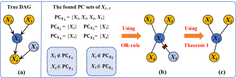
Figure 2: An example demonstrating how Theorem 1 is used.

As shown in Fig. 2 (a), node $X_{1}$ is the target variable. Due to the noise and small-scale samples, after using the PC learning algorithm, we may get $\textbf{PC}_{X_{1}}$=$\{X_{2},X_{3},X_{4},X_{5}\}$, $\textbf{PC}_{X_{4}}$=$\{X_{5}\}$, and $\textbf{PC}_{X_{5}}$=$\{X_{4}\}$. According to the symmetry constraint, if we apply the AND rule, the correct causal edge of $X_{1}-X_{4}$ will be missing. Therefore, we initially adopt the OR rule to obtain a comprehensive causal skeleton, as shown in Fig. 2 (b). But, it will introduce the redundant causal edge of $X_{1}-X_{5}$. Since $X_{2},X_{3},X_{4}\in\textbf{PC}_{X_{1}}$ and $X_{5}\notin\textbf{PC}_{X_{1}}$, it follows by Theorem 1 that $\mathcal{S}(X_{2}\rightarrow X_{1},\mathcal{D})-\mathcal{S}(\phi\rightarrow X_{1},\mathcal{D})=\mathcal{S}(X_{1}\rightarrow X_{2},\mathcal{D})-\mathcal{S}(\phi\rightarrow X_{2},\mathcal{D})>0$ holds (the same conclusion applies to nodes $X_{3}$ and $X_{4}$), and $\mathcal{S}(X_{5}\rightarrow X_{1},\mathcal{D})-\mathcal{S}(\phi\rightarrow X_{1},\mathcal{D})=\mathcal{S}(X_{1}\rightarrow X_{5},\mathcal{D})-\mathcal{S}(\phi\rightarrow X_{5},\mathcal{D})>0$ does not hold. Thus, based on the above distinction, the correct causal nodes in Fig. 2 (b) will be retained, while the non-causal nodes will be removed, resulting in the precise causal skeleton in Fig. 2 (c).

With Theorem 1, we can then maximize the local scores of the target nodes to remove the redundant skeleton during skeleton construction.

Since the scores of the equivalence class structure are the same, e.g. the score of $X\leftarrow T\rightarrow Y$ is $\mathcal{S}(\phi\to T,\mathcal{D})+\mathcal{S}(T\to X,\mathcal{D})+\mathcal{S}(T\to Y,\mathcal{D})$, and the score of $X\rightarrow T\rightarrow Y$ is $\mathcal{S}(\phi\to X,\mathcal{D})+\mathcal{S}(X\to T,\mathcal{D})+\mathcal{S}(T\to Y,\mathcal{D})$, by Theorem 1, $\mathcal{S}(\phi\to T,\mathcal{D})+\mathcal{S}(T\to X,\mathcal{D})=\mathcal{S}(\phi\to X,\mathcal{D})+\mathcal{S}(X\to T,\mathcal{D})$ holds, and the score of both are the same. Thus, in the following, we consider $X\rightarrow T\rightarrow Y$ as the representative of the equivalence class.

Theorem 2. Let $X,Y,T\in U$ and $T$ be a target node with no edge connected between $X$ and $Y$, and $X,Y\in\textbf{PC}_{T}$. If the score of local structures $X\rightarrow T\leftarrow Y$ is greater than the score of local structures $X\rightarrow T\rightarrow Y$, i.e., $\mathcal{S}(\phi\rightarrow X,\mathcal{D})+\mathcal{S}(\phi\rightarrow Y,\mathcal{D})+\mathcal{S}(X,Y\rightarrow T,\mathcal{D})>\mathcal{S}(\phi\rightarrow X,\mathcal{D})+\mathcal{S}(X\rightarrow T,\mathcal{D})+\mathcal{S}(T\rightarrow Y,\mathcal{D})$, then there exists a V-structure in variables $X$, $Y$, $T$, and $T$ is a collision node.

Proof: Assuming that the local structure $X\rightarrow T\leftarrow Y$ is the correct local causal network, denoted as $\mathcal{G}$, and $X\rightarrow T\rightarrow Y$ is denoted $\mathcal{G}^{\prime}$. The AIC score for ${\mathcal{S}}(\mathcal{G},\mathcal{D})-{\mathcal{S}}(\mathcal{G}^{\prime},\mathcal{D})$ is calculated as follows:

$${\mathcal{S}} (\mathcal{G},\mathcal{D})-{\mathcal{S}}(\mathcal{G}^{\prime},\mathcal{D})=$$ (6)

$$\mathcal{S}(\phi\to X,\mathcal{D})+\mathcal{S}(\phi\to Y,\mathcal{D})+\mathcal{S}(X,Y\to T,\mathcal{D})$$

$$-\mathcal{S}(\phi\to X,\mathcal{D})-\mathcal{S}(X\to T,\mathcal{D})-\mathcal{S}(T\to Y,\mathcal{D})$$

Subtracting the same terms, the log-likelihood terms are written in multiplicative form and using probabilities instead of ${\frac{{{N_{ijk}}}}{{{N_{ij}}}}}$, the following equation can be obtained:

$${\mathcal{S}}(\mathcal{G},\mathcal{D})-{\mathcal{S}}(\mathcal{G}^{\prime},\mathcal{D})=$$ (7)

$$[(\prod\limits_{k=1}^{{r_{Y}}}{p{{(Y|\phi)}^{{N_{k}}}}}\prod\limits_{j=1}^{{q_{T}}}{\prod\limits_{k=1}^{{r_{T}}}{p{{(T|X,Y)}^{{N_{jk}}}}}})/(\prod\limits_{j=1}^{{q_{T}}}{\prod\limits_{k=1}^{{r_{T}}}{p{{(T|X)}^{{N_{jk}}}}}}$$

$$\prod\limits_{j=1}^{{q_{Y}}}{\prod\limits_{k=1}^{{r_{Y}}}{p{{(Y|T)}^{{N_{jk}}}}}})]+\Delta(\mathcal{D},\mathcal{G}^{\prime})-\Delta(\mathcal{D},\mathcal{G})$$

Since the local structure $X\rightarrow T\leftarrow Y$ is the correct causal network, according to the Markov Condition of BN, ${p(Y|T)}$ can be written as $p(T|Y)p(Y)/p(T)$. The above equation can be transformed as follows:

$${\mathcal{S}}(\mathcal{G},\mathcal{D})-{\mathcal{S}}(\mathcal{G}^{\prime},\mathcal{D})=$$ (8)

$$[\prod\limits_{j=1}^{{q_{T}}}{\prod\limits_{k=1}^{{r_{T}}}{p{{(T|X,Y)}^{{N_{jk}}}}}}/\prod\limits_{j=1}^{{q_{T}}}{\prod\limits_{k=1}^{{r_{T}}}{p{{(T|X)}^{{N_{jk}}}}}}]/[\prod\limits_{j=1}^{{q_{T}}}{\prod\limits_{k=1}^{{r_{T}}}{p{{(T|Y)}^{{N_{jk}}}}}}$$

$$/\prod\limits_{k=1}^{{r_{T}}}{p{{(T|\phi)}^{{N_{k}}}}}]+\Delta(\mathcal{D},\mathcal{G}^{\prime})-\Delta(\mathcal{D},\mathcal{G})$$

$$=[{\mathcal{S}_{LL}}(X\to T\leftarrow Y|\mathcal{D})-{\mathcal{S}_{LL}}(X\to T)]-[{\mathcal{S}_{LL}}(Y\to T|\mathcal{D})$$

$$-{\mathcal{S}_{LL}}(\phi\to T)]+\Delta(\mathcal{D},\mathcal{G}^{\prime})-\Delta(\mathcal{D},\mathcal{G})$$

where $[{\mathcal{S}_{LL}}(X\to T\leftarrow Y|\mathcal{D})-{\mathcal{S}_{LL}}(X\to T)]$ can be viewed as the score by which ${\mathcal{S}_{LL}}(X\to T)$ increases when one $Y$ is added. Similarly, $[{\mathcal{S}_{LL}}(Y\to T|\mathcal{D})-{\mathcal{S}_{LL}}(\phi\to T)]$ can be viewed as the score that ${\mathcal{S}_{LL}}(\phi\to T)$ increases by adding one $Y$. But they are different in that $[{\mathcal{S}_{LL}}(X\to T\leftarrow Y|\mathcal{D})-{\mathcal{S}_{LL}}(X\to T)]$ has one more node $X$ compared to $[{\mathcal{S}_{LL}}(Y\to T|\mathcal{D})-{\mathcal{S}_{LL}}(\phi\to T)]$, and $X\in\textbf{P}_{T}$. According to score consistency, $[{\mathcal{S}_{LL}}(X\to T\leftarrow Y|\mathcal{D})-{\mathcal{S}_{LL}}(X\to T)]$ contains more parameters $\Theta$ compared to $[{\mathcal{S}_{LL}}(Y\to T|\mathcal{D})-{\mathcal{S}_{LL}}(\phi\to T)]$, so $[{\mathcal{S}_{LL}}(X\to T\leftarrow Y|\mathcal{D})-{\mathcal{S}_{LL}}(X\to T)]-[{\mathcal{S}_{LL}}(Y\to T|\mathcal{D})-{\mathcal{S}_{LL}}(\phi\to T)]>0$. Moreover, since $\Delta$ is a penalizes graph complexity and $\Delta(\mathcal{D},\mathcal{G}^{\prime})-\Delta(\mathcal{D},\mathcal{G})={r_{X}}{r_{T}}+{r_{Y}}{r_{T}}+{r_{X}}{r_{Y}}+1-{r_{X}}-{r_{T}}-{r_{Y}}-{r_{X}}{r_{T}}{r_{Y}}$. Thus, if the score of local structure $X\rightarrow T\leftarrow Y$ is still higher than the local structure of $X\rightarrow T\rightarrow Y$ after considering the graph complexity, we consider that $X$, $Y$, $T$ forms a V-structure and that $T$ is a collision node.

Similarly, assuming that $X\rightarrow T\rightarrow Y$ is the real local causal structure, denoted as $\mathcal{G}^{\prime}$, and $X\rightarrow T\leftarrow Y$ is denoted $\mathcal{G}$. The AIC score for ${\mathcal{S}}(\mathcal{G},\mathcal{D})-{\mathcal{S}}(\mathcal{G}^{\prime},\mathcal{D})$ is calculated as follows:

$${\mathcal{S}}(\mathcal{G},\mathcal{D})-{\mathcal{S}}(\mathcal{G}^{\prime},\mathcal{D})$$ (9)

$$= [(\prod\limits_{j=1}^{{q_{T}}}{\prod\limits_{k=1}^{{r_{T}}}{p{{(T|X,Y)}^{{N_{jk}}}}\prod\limits_{k=1}^{{r_{Y}}}{p{{(Y|\phi)}^{{N_{k}}}}}}})/(\prod\limits_{j=1}^{{q_{T}}}{\prod\limits_{k=1}^{{r_{T}}}{p{{(T|X)}^{{N_{jk}}}}}}$$

$$\prod\limits_{j=1}^{{q_{Y}}}{\prod\limits_{k=1}^{{r_{Y}}}{p{{(Y|T)}^{{N_{jk}}}}}})]+\Delta(\mathcal{D},\mathcal{G}^{\prime})-\Delta(\mathcal{D},\mathcal{G})$$

$$= [\prod\limits_{j=1}^{{q_{Y}}}{\prod\limits_{k=1}^{{r_{Y}}}{p{{(Y|(T|X))}^{{N_{jk}}}}}}/\prod\limits_{j=1}^{{q_{Y}}}{\prod\limits_{k=1}^{{r_{Y}}}{p{{(Y|T)}^{{N_{jk}}}}}}]+\Delta(\mathcal{D},\mathcal{G}^{\prime})$$

$$-\Delta(\mathcal{D},\mathcal{G})$$

At this point, the structures $(X\rightarrow T)\rightarrow Y$ and $T\to Y$ contain the $X\to Y$ parameter $\Theta$, but $T\to Y$ has less $X\to T$ parameters $\Theta$ than $(X\to T)\to Y$. Therefore, according to the second article of score consistency, the score of $T\to Y$ is higher than that of $(X\to T)\to Y$. Similarly, if the score of local structure $X\rightarrow T\rightarrow Y$ is still greater than the local structure of $X\rightarrow T\leftarrow Y$ after considering the $\Delta$, we consider node $X$, $Y$, $Z$ to be the equivalence class. $\hfill\blacksquare$

For BDeu score fuction, $X\rightarrow T\leftarrow Y$ and $X\rightarrow T\rightarrow Y$ have the same prior graph probability $p(\mathcal{G})/p(\mathcal{G}^{\prime})$, and it satisfies score consistency. Thus, the same conclusion can be drawn if the maximum posterior probability of $X\rightarrow T\leftarrow Y$ is greater or less than $X\rightarrow T\rightarrow Y$ when the prior parameter $\Theta$ distribution is considered.

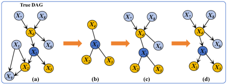
Figure 3: An example demonstrating how Theorem 2 is used.

As shown in Fig. 3 (a), the node $X_{1}$ is the target variable and after using the PC learning algorithm, we get $\textbf{PC}_{X_{1}}$=$\{X_{2},X_{3},X_{4}\}$. Since $X_{1}$ and its PC nodes are an equivalence class structure. Thus, according to Theorem 2, the scores of the local structures $X_{2}\rightarrow X_{1}\rightarrow X_{3}$, $X_{2}\rightarrow X_{1}\rightarrow X_{4}$, and $X_{3}\rightarrow X_{1}\rightarrow X_{4}$ will be higher than those of $X_{2}\rightarrow X_{1}\leftarrow X_{3}$, $X_{2}\rightarrow X_{1}\leftarrow X_{4}$, and $X_{3}\rightarrow X_{1}\leftarrow X_{4}$. At this point, we obtain the undirected local structure of Fig. 3 (b) and continue to extend the learning outward. Then, the node $X_{4}$ becomes the target variable. By PC learning algorithm, we get $\textbf{PC}_{X_{4}}$=$\{X_{1},X_{6},X_{7},X_{8}\}$. According to Theorem 2, the local structure $X_{7}\rightarrow X_{4}\leftarrow X_{8}$ will have a higher score than $X_{7}\rightarrow X_{4}\rightarrow X_{8}$, so nodes $X_{7}$ and $X_{8}$ will be directed to $X_{4}$. Moreover, the remaining equivalence class structure’s score will be higher than its V-structure’s. Thus, nodes $X_{1}$ and $X_{6}$ will not be oriented and we obtain the local causal structure in Fig. 3 (c). Finally, we can obtain the local causal structure in Fig. 3 (d) with Meek-rule. At this point, the direct cause and effect of node $X_{1}$ are distinguished. We stop extending learning outward.

With Theorem 2, we can gradually identify the final causal direction by scoring to recognize the V-structure, while avoiding the disruption of equivalence classes.

4.2 Detailed descriptions of the HLCD algorithm

In this section, we present the proposed HLCD algorithm through the theoretical analysis in the previous section.

Step 1: Hybrid-based local causal skeleton construction (Lines 2-14): HLCD first pops a variable at the front of the queue $Q$ and assigns it to the current iteration node $Z$ (initially $Z$ is the given target $T$) (Line 4). Then, HLCD uses the constraint-based PC discovery algorithm to find the $\textbf{PC}_{Z}$ and constructs a local causal skeleton with the OR rule (Line 6). As we do not need MBs and separating sets for the edge orientation phase, HLCD can use any of the state-of-the-art PC discovery algorithms, such as MMPC, HITION-PC, FCBF, etc. Then, the HLCD stores $Z$ into V to prevent repeated learning of the PC of variables (line 7). At this point, HLCD builds an initial local causal skeleton from the OR rule and learned PC sets.

As the OR rule can generate a comprehensive but redundant causal skeleton, HLCD uses the score-based method to eliminate redundant causal skeletons, ensuring they don’t interfere with subsequent causal orientations. With the analysis of Theorem 1, if node $X\in\textbf{PC}_{Z}$, then the following $\mathcal{S}(X\rightarrow Z,\mathcal{D})-\mathcal{S}(\phi\rightarrow Z,\mathcal{D})=\mathcal{S}(Z\rightarrow X,\mathcal{D})-\mathcal{S}(\phi\rightarrow X,\mathcal{D})>0$ will be hold. HLCD does this by testing each variable $X$ in $\textbf{PC}_{Z}$ to see if it satisfies Theorem 1, and removing it from $\textbf{PC}_{Z}$ if it does not satisfy (Lines 9-13). Then, HLCD pushes all variables in $\textbf{PC}_{Z}$ into $Q$ to recursively find the PC of each node in $\textbf{PC}_{Z}$ in the next iterations for expanding (Line 14). At the end of step 1, HLCD obtains the accurate local causal skeleton consisting of all nodes in the set V and their PC nodes.

1

2

Input: $\mathcal{D}$: Data, $T$: The target variable;

Output: $[\textbf{P}_{T},\textbf{C}_{T},\textbf{UN}_{T}]$: Local causal structure of $T$ ;

3

4Initialize: $\textbf{V}=\emptyset$, $Q=\{T\}$;

5

6repeat

7   

8   /*Step 1: Hybrid-based local causal skeleton construction*/  

9   $Z=Q.pop$;  

10   if $Z\notin\textbf{V}$ then

11      

12      $\textbf{PC}_{Z}$ = getPC($\mathcal{D}$,$Z$);  

13      $\textbf{V}=\textbf{V}\cup\{Z\}$;  

14    end if

15   

16   for each $X\in\bf{PC_{Z}}$ do

17      

18      if The local score of $X\to Z$ is not equal to $Z\to X$ or $\mathcal{S}(X\to Z,\mathcal{D})-\mathcal{S}(\phi\to Z,\mathcal{D})<0$ then

19         

20         $\textbf{PC}_{Z}=\textbf{PC}_{Z}\backslash\{X\}$;  

21       end if

22      

23    end for

24   

25   $Q=Q.push(\textbf{PC}_{Z}\backslash\{\textbf{V}\})$;  

26   /*Step 2: Hybrid-based local causal orientation*/  

27   for each $X$,$Y\in\textbf{PC}_{Z}$ do

28      

29      if The local score of $X\rightarrow Z\leftarrow Y$ is greater than $X\rightarrow Z\rightarrow Y$ then

30         

31         The $X$, $Y$, $Z$ form a V-structure, and $Z$ is the collision node;  

32       end if

33      

34    end for

35   

36   Using Meek-rule to orient edge orientations between variables in V;  

37until All causal orientations of $T$ is determined, or $Q=\emptyset$, or $\textbf{V}=\textbf{U}$;

38Return $[\textbf{P}_{T},\textbf{C}_{T},\textbf{UN}_{T}]$;  

Algorithm 1 Hybrid Local Causal Discovery

Step 2: Hybrid-based local causal orientation (Lines 15-22): To avoid the effect of the score equivalence, HLCD distinguishes between V-structures and equivalence class structures by employing the score-based method. Specifically, HLCD identifies the V-structures in the causal skeleton by comparing the two local structure scores of each tuple $X$, $Y$ and $Z$ ($X,Y\in\textbf{PC}_{Z}$) in the causal skeleton obtained in step 1. If $\mathcal{S}(\phi\rightarrow X,\mathcal{D})+\mathcal{S}(\phi\rightarrow Y,\mathcal{D})+\mathcal{S}(X,Y\rightarrow Z,\mathcal{D})>\mathcal{S}(\phi\rightarrow X,\mathcal{D})+\mathcal{S}(X\rightarrow Z,\mathcal{D})+\mathcal{S}(Z\rightarrow Y,\mathcal{D})$, then the edge $X-Z$ and edge $Y-Z$ will be oriented as $X\rightarrow Z$ and $Y\rightarrow Z$ (Lines 16-20). It may be the V-structure consisting of $Z$ and $\textbf{P}_{Z}$, or consisting of $Z$ and $\textbf{C}_{Z}$ and spouse nodes. At this point, HLCD orients the causal orientations of all V-structures in the current causal skeleton and does not orient the causal orientations of equivalent class structures.

Finally, HLCD uses the constraint-based Meek-rule as well as the discovered V-structure to orient the causal orientations of the nodes in the set V (Line 21). If all causal orientations of the $T$ are recognized in the current V, learning stops, otherwise it continues to expand outward until it distinguishes between the father and child nodes of the $T$ (Line 22).

Theorem 3 (Correctness of HLCD). Given a set of i.i.d data $\mathcal{D}$, and samples from some distribution ${\mathcal{P}}$. HLCD distinguishes all parents from children of a given variable.

Proof: According to Theorem 1, if $X\in\textbf{PC}_{T}$, the local scores of $X\rightarrow T$ and $T\rightarrow X$ are the same and higher than $\phi\rightarrow T$ and $\phi\rightarrow X$. Therefore, Step 1 will keep all the true PCs found by the PC discovery algorithm and remove the false positive nodes. In the local skeleton, if $X,Y\in\textbf{P}_{T}$, the local score of $X\rightarrow T\leftarrow Y$ is higher than that of $X\rightarrow T\rightarrow Y$ according to Theorem 2. Thus, Step 2 will find all correct V-structures in the local skeleton and will not orient the edge directions of the equivalence classes. At this point, $T$ and all its parent nodes are found correctly. Finally, the child nodes oriented out of the Meek-rule are correct. Thus, all the parents and children of a given target variable distinguished by HLCD are correct.

5 Experiments

In this section, we conduct experiments to evaluate the performance of our method. In Section 5.1, we describe the experiment settings. In Section 5.2, we provide detailed experimental figures, and the results are analyzed.

5.1 Experimental settings

5.1.1 Datasets

TABLE I: Summary of benchmark BN datasets

	Num.	Num.	Min/Max	Max In/Out	Domain
Network	Vars	Edges	$|$PCset$|$	Degree	Range
Alarm	37	46	1/6	4/5	2-4
Alarm3	111	149	1/6	4/5	2-4
Alarm5	185	265	1/8	4/6	2-4
Alarm10	370	570	1/9	4/7	2-4
Child	20	25	1/8	2/7	2-6
Insurance3	81	163	1/9	4/7	2-5
Insurance5	135	281	1/10	5/8	2-5
Hailfinder3	168	283	1/19	5/18	2-11
Hailfinder5	280	458	1/19	5/19	2-11
Hailfinder10	560	283	1/21	5/20	2-11
Barley	48	84	1/8	4/5	2-67
Link	724	1125	0/17	3/14	2-4
Pigs	441	592	1/41	2/39	3-3
Gene	801	972	0/11	4/10	3-5

We use 14 benchmark BNs to evaluate HLCD against its rivals. Each benchmark BN contains two groups of data: one with 10 datasets of 500 samples and another with 10 datasets of 1000 samples. A brief description of the 14 BNs is listed in Table 1.

5.1.2 Comparison methods

We compare our approaches to HLCD with seven state-of-the-art local causal discovery algorithms, including PCD-by-PCD [23], MB-by-MB [25], CMB [26], LCS-FS [28], ELCS [30], GraN-LCS [14], and the partially causal structured discovery algorithm PSL  [31].

5.1.3 Evaluation metrics

We evaluate the performance of HLCD with its competitors in terms of structural correctness, structural errors and efficiency. The F1 and SHD metric shown below are used to measure structural correctness and error, respectively. Finally the running time are used as a measure of the efficiency of the algorithm.

• $F1$: ($F1=2*Precision*Recall/(Precision+Recall)$). $Precision$ denotes the number of correctly predicted edges in the causal direction in the output divided by the total number of edges in the output of the algorithm, while $recall$ denotes the number of correctly predicted edges in the causal direction in the output divided by the total number of edges in the true DAG.

• $SHD$: $SHD$ is the number of total error edges, which contains $Undirected$, $Reverse$ , $Miss$ and $Extra$. They are the number of undirected edges, reversed edges, missing edges, and extra edges in the learned local DAG compared to the true DAG. The smaller value of SHD is better.

• $Time$: $Time$ is the running time (in seconds) of the local causal discovery algorithm.

In the following Tables, the results are reported in the format of $A\pm B$, where $A$ denotes the average results, and $B$ represents the standard deviation. The best results in each setting have been marked in bold. “-” means that the algorithm does not get the result in 72 hours.

5.1.4 Implementation details

All the code implementations are done in Matlab or Python [35], and the experiments are conducted on a computer with an Intel Core i7-12700 CPU and 8GB of memory. The significance level for the CI tests is set at 0.01 and the threshold for mutual information is set at 0.03. Furthermore, PCD-by-PCD is using the MMPC [36] in the skeleton construction stage. MB-by-MB uses IAMB [37] to obtain the MBs. CMB uses HITON-MB [27] to obtain MBs. LCS-FS uses FCBF [29] for skeleton construction. ELCS uses HITONPC [27] for skeleton construction. PSL uses PCsimple [38] to obtain the skeleton. Therefore, to avoid the disparities in results caused by the PC algorithm, we keep the PC algorithm used by HLCD consistent with its comparison algorithms and compare the experimental results separately.

5.2 Experimental results

In this section, we report the experimental results of HLCD with its rivals on 14 BN datasets. Section 5.2.1 reports structural correctness and structural errors, Section 5.2.2 focuses on the time efficiency of the algorithms, and Section 5.2.3 performs ablation experiments to verify the performance of Theorem 1 and Theorem 2, respectively.

5.2.1 Structural correctness and errors

TABLE II: Summary of structural correctness and errors for HLCD-FS, LCS-FS, and MB-by-MB

		Size=500			Size=500					Size=1000			Size=1000
Network	Algorithm	F1 (↑)	Precision (↑)	Recall (↑)	SHD (↓)	Undirected (↓)	Reverse (↓)	Miss (↓)	Extra (↓)	F1 (↑)	Precision (↑)	Recall (↑)	SHD (↓)	Undirected (↓)	Reverse (↓)	Miss (↓)	Extra (↓)
Alarm	MB-by-MB	0.52$\pm$0.06	0.55$\pm$0.05	0.52$\pm$0.06	1.69$\pm$0.12	0.07$\pm$0.08	0.46$\pm$0.09	0.73$\pm$0.07	0.43$\pm$0.07	0.57$\pm$0.04	0.58$\pm$0.05	0.60$\pm$0.03	1.59$\pm$0.17	0.20$\pm$0.16	0.40$\pm$0.09	0.49$\pm$0.05	0.50$\pm$0.14
	LCS-FS	0.44$\pm$0.05	0.48$\pm$0.05	0.43$\pm$0.05	1.75$\pm$0.11	0.33$\pm$0.11	0.25$\pm$0.08	0.80$\pm$0.05	0.38$\pm$0.08	0.55$\pm$0.04	0.59$\pm$0.04	0.54$\pm$0.04	1.47$\pm$0.13	0.22$\pm$0.11	0.29$\pm$0.11	0.63$\pm$0.04	0.34$\pm$0.06
	HLCD-FS	0.58$\pm$0.02	0.63$\pm$0.02	0.57$\pm$0.03	1.43$\pm$0.11	0.09$\pm$0.04	0.14$\pm$0.05	0.80$\pm$0.05	0.40$\pm$0.07	0.64$\pm$0.03	0.68$\pm$0.04	0.63$\pm$0.03	1.18$\pm$0.12	0.14$\pm$0.04	0.06$\pm$0.05	0.63$\pm$0.05	0.34$\pm$0.07
Alarm3	MB-by-MB	0.46$\pm$0.03	0.50$\pm$0.03	0.45$\pm$0.03	2.07$\pm$0.09	0.06$\pm$0.05	0.50$\pm$0.07	0.99$\pm$0.04	0.52$\pm$0.06	0.43$\pm$0.01	0.43$\pm$0.02	0.47$\pm$0.01	2.44$\pm$0.10	0.04$\pm$0.04	0.71$\pm$0.07	0.72$\pm$0.02	0.97$\pm$0.08
	LCS-FS	0.53$\pm$0.02	0.61$\pm$0.03	0.50$\pm$0.02	1.51$\pm$0.06	0.23$\pm$0.06	0.32$\pm$0.08	0.78$\pm$0.03	0.20$\pm$0.05	0.56$\pm$0.02	0.63$\pm$0.02	0.53$\pm$0.03	1.34$\pm$0.08	0.31$\pm$0.06	0.22$\pm$0.03	0.66$\pm$0.02	0.15$\pm$0.04
	HLCD-FS	0.61$\pm$0.03	0.70$\pm$0.04	0.57$\pm$0.03	1.29$\pm$0.08	0.20$\pm$0.12	0.12$\pm$0.07	0.77$\pm$0.03	0.19$\pm$0.05	0.62$\pm$0.03	0.69$\pm$0.03	0.58$\pm$0.03	1.20$\pm$0.08	0.27$\pm$0.11	0.12$\pm$0.04	0.65$\pm$0.03	0.15$\pm$0.04
Alarm5	MB-by-MB	0.43$\pm$0.03	0.48$\pm$0.03	0.42$\pm$0.03	2.48$\pm$0.10	0.03$\pm$0.02	0.56$\pm$0.04	1.18$\pm$0.03	0.70$\pm$0.06	0.39$\pm$0.02	0.39$\pm$0.02	0.43$\pm$0.02	2.91$\pm$0.08	0.02$\pm$0.01	0.79$\pm$0.04	0.94$\pm$0.02	1.17$\pm$0.07
	LCS-FS	0.50$\pm$0.04	0.58$\pm$0.04	0.47$\pm$0.04	1.81$\pm$0.09	0.26$\pm$0.10	0.32$\pm$0.05	0.96$\pm$0.02	0.27$\pm$0.04	0.57$\pm$0.04	0.64$\pm$0.04	0.53$\pm$0.03	1.54$\pm$0.09	0.25$\pm$0.09	0.25$\pm$0.03	0.85$\pm$0.02	0.19$\pm$0.03
	HLCD-FS	0.57$\pm$0.02	0.66$\pm$0.03	0.54$\pm$0.02	1.60$\pm$0.05	0.17$\pm$0.07	0.20$\pm$0.03	0.96$\pm$0.02	0.27$\pm$0.03	0.58$\pm$0.02	0.65$\pm$0.02	0.54$\pm$0.02	1.47$\pm$0.07	0.23$\pm$0.04	0.22$\pm$0.03	0.83$\pm$0.02	0.19$\pm$0.03
Alarm10	MB-by-MB	0.36$\pm$0.02	0.42$\pm$0.02	0.36$\pm$0.02	2.97$\pm$0.08	0.01$\pm$0.01	0.64$\pm$0.03	1.42$\pm$0.02	0.89$\pm$0.05	0.33$\pm$0.01	0.33$\pm$0.01	0.39$\pm$0.01	3.59$\pm$0.05	0.00$\pm$0.00	0.89$\pm$0.03	1.14$\pm$0.02	1.55$\pm$0.04
	LCS-FS	0.49$\pm$0.02	0.57$\pm$0.02	0.45$\pm$0.01	2.19$\pm$0.07	0.17$\pm$0.04	0.39$\pm$0.03	1.17$\pm$0.02	0.47$\pm$0.07	0.56$\pm$0.02	0.65$\pm$0.02	0.52$\pm$0.02	1.82$\pm$0.05	0.16$\pm$0.05	0.29$\pm$0.03	1.02$\pm$0.01	0.35$\pm$0.03
	HLCD-FS	0.57$\pm$0.02	0.67$\pm$0.02	0.53$\pm$0.01	1.95$\pm$0.07	0.09$\pm$0.04	0.23$\pm$0.02	1.17$\pm$0.02	0.47$\pm$0.07	0.59$\pm$0.01	0.68$\pm$0.01	0.55$\pm$0.01	1.73$\pm$0.04	0.14$\pm$0.03	0.23$\pm$0.02	1.01$\pm$0.01	0.35$\pm$0.03
Child	MB-by-MB	0.42$\pm$0.23	0.46$\pm$0.26	0.43$\pm$0.22	1.91$\pm$0.45	0.39$\pm$0.57	0.47$\pm$0.20	0.78$\pm$0.12	0.27$\pm$0.05	0.51$\pm$0.13	0.51$\pm$0.14	0.52$\pm$0.13	1.79$\pm$0.28	0.25$\pm$0.48	0.67$\pm$0.26	0.53$\pm$0.06	0.34$\pm$0.13
	LCS-FS	0.30$\pm$0.20	0.32$\pm$0.22	0.29$\pm$0.19	1.85$\pm$0.53	1.16$\pm$0.64	0.17$\pm$0.17	0.45$\pm$0.07	0.07$\pm$0.04	0.30$\pm$0.13	0.31$\pm$0.14	0.29$\pm$0.13	1.82$\pm$0.36	1.24$\pm$0.43	0.12$\pm$0.12	0.45$\pm$0.08	0.01$\pm$0.03
	HLCD-FS	0.68$\pm$0.11	0.75$\pm$0.11	0.65$\pm$0.11	0.99$\pm$0.23	0.11$\pm$0.17	0.33$\pm$0.08	0.49$\pm$0.08	0.06$\pm$0.04	0.54$\pm$0.16	0.59$\pm$0.19	0.51$\pm$0.16	1.20$\pm$0.46	0.31$\pm$0.56	0.27$\pm$0.18	0.28$\pm$0.13	0.34$\pm$0.09
Insurance3	MB-by-MB	0.37$\pm$0.02	0.47$\pm$0.04	0.33$\pm$0.02	3.35$\pm$0.14	0.01$\pm$0.01	0.82$\pm$0.08	2.07$\pm$0.03	0.45$\pm$0.09	0.41$\pm$0.03	0.48$\pm$0.03	0.39$\pm$0.02	3.24$\pm$0.12	0.02$\pm$0.02	0.90$\pm$0.06	1.75$\pm$0.05	0.57$\pm$0.07
	LCS-FS	0.46$\pm$0.03	0.55$\pm$0.04	0.42$\pm$0.03	2.73$\pm$0.15	0.19$\pm$0.10	0.57$\pm$0.09	1.62$\pm$0.05	0.35$\pm$0.09	0.54$\pm$0.02	0.67$\pm$0.02	0.47$\pm$0.02	2.42$\pm$0.09	0.13$\pm$0.04	0.43$\pm$0.06	1.65$\pm$0.06	0.21$\pm$0.04
	HLCD-FS	0.52$\pm$0.03	0.63$\pm$0.03	0.47$\pm$0.03	2.58$\pm$0.14	0.03$\pm$0.09	0.59$\pm$0.09	1.61$\pm$0.04	0.35$\pm$0.08	0.56$\pm$0.02	0.70$\pm$0.02	0.49$\pm$0.02	2.42$\pm$0.08	0.00$\pm$0.00	0.57$\pm$0.05	1.65$\pm$0.06	0.20$\pm$0.03
Insurance5	MB-by-MB	0.33$\pm$0.02	0.43$\pm$0.03	0.30$\pm$0.02	3.69$\pm$0.10	0.01$\pm$0.01	0.87$\pm$0.03	2.29$\pm$0.04	0.53$\pm$0.06	0.35$\pm$0.01	0.42$\pm$0.02	0.34$\pm$0.01	3.70$\pm$0.11	0.00$\pm$0.00	1.04$\pm$0.05	1.94$\pm$0.03	0.72$\pm$0.06
	LCS-FS	0.47$\pm$0.02	0.58$\pm$0.03	0.43$\pm$0.02	2.96$\pm$0.10	0.16$\pm$0.05	0.51$\pm$0.06	1.83$\pm$0.05	0.46$\pm$0.08	0.52$\pm$0.02	0.66$\pm$0.02	0.45$\pm$0.02	2.61$\pm$0.07	0.19$\pm$0.04	0.37$\pm$0.05	1.85$\pm$0.04	0.19$\pm$0.03
	HLCD-FS	0.50$\pm$0.02	0.61$\pm$0.04	0.45$\pm$0.02	2.90$\pm$0.09	0.05$\pm$0.07	0.57$\pm$0.06	1.83$\pm$0.06	0.45$\pm$0.07	0.54$\pm$0.02	0.69$\pm$0.03	0.47$\pm$0.02	2.63$\pm$0.09	0.03$\pm$0.07	0.56$\pm$0.03	1.85$\pm$0.04	0.19$\pm$0.03
Barley	MB-by-MB	0.00$\pm$0.00	0.00$\pm$0.00	0.00$\pm$0.00	3.75$\pm$0.04	0.71$\pm$0.01	0.00$\pm$0.00	2.79$\pm$0.01	0.25$\pm$0.04	0.07$\pm$0.02	0.12$\pm$0.03	0.05$\pm$0.02	3.70$\pm$0.06	0.59$\pm$0.08	0.04$\pm$0.04	2.71$\pm$0.04	0.37$\pm$0.03
	LCS-FS	0.24$\pm$0.02	0.25$\pm$0.02	0.24$\pm$0.03	4.33$\pm$0.10	0.05$\pm$0.07	0.54$\pm$0.10	1.98$\pm$0.07	1.76$\pm$0.09	0.32$\pm$0.02	0.34$\pm$0.02	0.32$\pm$0.02	3.77$\pm$0.11	0.09$\pm$0.06	0.54$\pm$0.08	1.88$\pm$0.04	1.26$\pm$0.07
	HLCD-FS	0.29$\pm$0.05	0.38$\pm$0.06	0.25$\pm$0.05	3.05$\pm$0.15	0.20$\pm$0.06	0.27$\pm$0.03	2.14$\pm$0.04	0.45$\pm$0.07	0.36$\pm$0.02	0.44$\pm$0.03	0.33$\pm$0.02	2.98$\pm$0.08	0.17$\pm$0.00	0.37$\pm$0.05	1.92$\pm$0.05	0.53$\pm$0.03
Hailfinder3	MB-by-MB	0.23$\pm$0.01	0.34$\pm$0.02	0.20$\pm$0.01	4.16$\pm$0.04	0.33$\pm$0.02	0.33$\pm$0.03	2.10$\pm$0.02	1.40$\pm$0.03	0.26$\pm$0.01	0.34$\pm$0.01	0.25$\pm$0.01	3.22$\pm$0.05	0.21$\pm$0.02	0.45$\pm$0.04	1.99$\pm$0.02	0.57$\pm$0.03
	LCS-FS	0.32$\pm$0.02	0.42$\pm$0.03	0.28$\pm$0.02	3.02$\pm$0.06	0.17$\pm$0.06	0.46$\pm$0.04	1.73$\pm$0.03	0.66$\pm$0.05	0.39$\pm$0.04	0.51$\pm$0.05	0.38$\pm$0.04	2.90$\pm$0.12	0.23$\pm$0.08	0.27$\pm$0.05	1.76$\pm$0.03	0.64$\pm$0.05
	HLCD-FS	0.43$\pm$0.04	0.55$\pm$0.05	0.40$\pm$0.05	2.89$\pm$0.14	0.36$\pm$0.09	0.11$\pm$0.02	1.77$\pm$0.03	0.64$\pm$0.07	0.45$\pm$0.02	0.58$\pm$0.02	0.41$\pm$0.02	2.79$\pm$0.06	0.26$\pm$0.06	0.18$\pm$0.04	1.81$\pm$0.03	0.54$\pm$0.03
Hailfinder5	MB-by-MB	0.23$\pm$0.01	0.31$\pm$0.01	0.20$\pm$0.01	4.13$\pm$0.02	0.34$\pm$0.02	0.38$\pm$0.03	1.99$\pm$0.01	1.42$\pm$0.01	0.25$\pm$0.01	0.32$\pm$0.01	0.24$\pm$0.01	3.20$\pm$0.03	0.21$\pm$0.01	0.52$\pm$0.03	1.87$\pm$0.01	0.60$\pm$0.03
	LCS-FS	0.34$\pm$0.01	0.42$\pm$0.02	0.31$\pm$0.02	2.96$\pm$0.06	0.22$\pm$0.03	0.44$\pm$0.03	1.58$\pm$0.04	0.72$\pm$0.06	0.41$\pm$0.03	0.50$\pm$0.03	0.40$\pm$0.03	2.76$\pm$0.05	0.24$\pm$0.05	0.28$\pm$0.04	1.61$\pm$0.02	0.63$\pm$0.03
	HLCD-FS	0.43$\pm$0.04	0.52$\pm$0.04	0.41$\pm$0.04	2.84$\pm$0.12	0.47$\pm$0.11	0.09$\pm$0.03	1.62$\pm$0.03	0.66$\pm$0.05	0.47$\pm$0.03	0.57$\pm$0.04	0.44$\pm$0.03	2.68$\pm$0.11	0.32$\pm$0.09	0.16$\pm$0.03	1.66$\pm$0.02	0.55$\pm$0.05
Hailfinder10	MB-by-MB	0.20$\pm$0.01	0.30$\pm$0.01	0.17$\pm$0.00	4.54$\pm$0.03	0.31$\pm$0.01	0.42$\pm$0.01	2.35$\pm$0.01	1.45$\pm$0.02	0.23$\pm$0.01	0.31$\pm$0.01	0.22$\pm$0.01	3.57$\pm$0.02	0.19$\pm$0.00	0.51$\pm$0.02	2.25$\pm$0.01	0.63$\pm$0.02
	LCS-FS	0.31$\pm$0.01	0.42$\pm$0.01	0.28$\pm$0.01	3.44$\pm$0.03	0.19$\pm$0.03	0.48$\pm$0.03	1.90$\pm$0.02	0.87$\pm$0.04	0.38$\pm$0.01	0.51$\pm$0.02	0.35$\pm$0.01	3.09$\pm$0.03	0.24$\pm$0.04	0.29$\pm$0.04	1.95$\pm$0.02	0.61$\pm$0.02
	HLCD-FS	0.43$\pm$0.02	0.58$\pm$0.02	0.39$\pm$0.02	3.03$\pm$0.05	0.23$\pm$0.05	0.25$\pm$0.02	1.95$\pm$0.02	0.59$\pm$0.03	0.44$\pm$0.01	0.59$\pm$0.01	0.39$\pm$0.01	2.90$\pm$0.03	0.21$\pm$0.04	0.21$\pm$0.02	1.97$\pm$0.02	0.50$\pm$0.02
Link	MB-by-MB	0.18$\pm$0.01	0.22$\pm$0.02	0.19$\pm$0.01	3.76$\pm$0.04	0.13$\pm$0.02	0.29$\pm$0.01	2.21$\pm$0.03	1.13$\pm$0.02	0.22$\pm$0.01	0.28$\pm$0.02	0.23$\pm$0.01	4.03$\pm$0.04	0.03$\pm$0.01	0.41$\pm$0.01	2.04$\pm$0.02	1.55$\pm$0.03
	LCS-FS	0.18$\pm$0.01	0.18$\pm$0.01	0.20$\pm$0.01	4.29$\pm$0.29	0.36$\pm$0.03	0.30$\pm$0.02	1.79$\pm$0.03	1.85$\pm$0.27	0.20$\pm$0.01	0.20$\pm$0.01	0.22$\pm$0.01	4.04$\pm$0.09	0.34$\pm$0.01	0.27$\pm$0.02	1.79$\pm$0.01	1.65$\pm$0.09
	HLCD-FS	0.20$\pm$0.02	0.21$\pm$0.02	0.22$\pm$0.02	4.09$\pm$0.25	0.34$\pm$0.03	0.20$\pm$0.01	1.82$\pm$0.03	1.73$\pm$0.21	0.22$\pm$0.00	0.22$\pm$0.01	0.24$\pm$0.00	3.90$\pm$0.10	0.33$\pm$0.00	0.17$\pm$0.01	1.79$\pm$0.01	1.61$\pm$0.10
Pigs	MB-by-MB	0.50$\pm$0.01	0.49$\pm$0.01	0.54$\pm$0.01	2.11$\pm$0.04	0.00$\pm$0.00	0.96$\pm$0.02	0.52$\pm$0.01	0.62$\pm$0.03	0.50$\pm$0.02	0.49$\pm$0.02	0.54$\pm$0.02	2.09$\pm$0.05	0.00$\pm$0.00	0.97$\pm$0.04	0.52$\pm$0.01	0.61$\pm$0.02
	LCS-FS	0.92$\pm$0.01	0.91$\pm$0.01	0.93$\pm$0.01	0.47$\pm$0.08	0.01$\pm$0.01	0.08$\pm$0.02	0.12$\pm$0.03	0.25$\pm$0.04	0.95$\pm$0.01	0.95$\pm$0.01	0.97$\pm$0.01	0.25$\pm$0.05	0.00$\pm$0.00	0.06$\pm$0.01	0.05$\pm$0.02	0.14$\pm$0.02
	HLCD-FS	0.96$\pm$0.01	0.96$\pm$0.01	0.96$\pm$0.01	0.26$\pm$0.06	0.01$\pm$0.00	0.01$\pm$0.01	0.13$\pm$0.03	0.12$\pm$0.03	0.97$\pm$0.01	0.97$\pm$0.01	0.99$\pm$0.01	0.18$\pm$0.05	0.00$\pm$0.00	0.00$\pm$0.00	0.05$\pm$0.02	0.13$\pm$0.03
Gene	MB-by-MB	0.26$\pm$0.01	0.25$\pm$0.01	0.30$\pm$0.01	2.63$\pm$0.04	0.00$\pm$0.00	1.21$\pm$0.02	0.51$\pm$0.01	0.91$\pm$0.02	0.28$\pm$0.00	0.27$\pm$0.00	0.31$\pm$0.01	2.56$\pm$0.01	0.00$\pm$0.00	1.19$\pm$0.01	0.48$\pm$0.01	0.89$\pm$0.01
	LCS-FS	0.91$\pm$0.01	0.92$\pm$0.01	0.91$\pm$0.01	0.30$\pm$0.04	0.07$\pm$0.03	0.09$\pm$0.02	0.08$\pm$0.01	0.07$\pm$0.01	0.94$\pm$0.01	0.95$\pm$0.01	0.93$\pm$0.01	0.21$\pm$0.02	0.07$\pm$0.03	0.04$\pm$0.01	0.08$\pm$0.01	0.03$\pm$0.00
	HLCD-FS	0.94$\pm$0.01	0.95$\pm$0.01	0.93$\pm$0.02	0.25$\pm$0.05	0.05$\pm$0.05	0.06$\pm$0.01	0.08$\pm$0.01	0.06$\pm$0.01	0.97$\pm$0.01	0.97$\pm$0.01	0.97$\pm$0.01	0.14$\pm$0.02	0.02$\pm$0.03	0.04$\pm$0.01	0.04$\pm$0.00	0.04$\pm$0.01

TABLE III: Summary of structural correctness and errors for HLCD-H, CMB, and ELCS

		Size=500			Size=500					Size=1000			Size=1000
Network	Algorithm	F1 (↑)	Precision (↑)	Recall (↑)	SHD (↓)	Undirected (↓)	Reverse (↓)	Miss (↓)	Extra (↓)	F1 (↑)	Precision (↑)	Recall (↑)	SHD (↓)	Undirected (↓)	Reverse (↓)	Miss (↓)	Extra (↓)
Alarm	CMB	0.43$\pm$0.09	0.44$\pm$0.09	0.43$\pm$0.09	1.83$\pm$0.23	0.25$\pm$0.23	0.65$\pm$0.06	0.49$\pm$0.09	0.44$\pm$0.08	0.50$\pm$0.07	0.52$\pm$0.07	0.50$\pm$0.08	1.44$\pm$0.19	0.16$\pm$0.15	0.75$\pm$0.10	0.34$\pm$0.07	0.20$\pm$0.07
	ELCS	0.44$\pm$0.04	0.47$\pm$0.05	0.43$\pm$0.04	1.76$\pm$0.14	0.46$\pm$0.08	0.36$\pm$0.04	0.52$\pm$0.05	0.42$\pm$0.08	0.66$\pm$0.05	0.69$\pm$0.05	0.65$\pm$0.06	0.92$\pm$0.16	0.34$\pm$0.09	0.08$\pm$0.04	0.34$\pm$0.07	0.16$\pm$0.05
	HLCD-H	0.64$\pm$0.05	0.66$\pm$0.05	0.65$\pm$0.05	1.27$\pm$0.15	0.21$\pm$0.08	0.15$\pm$0.10	0.49$\pm$0.06	0.43$\pm$0.08	0.72$\pm$0.05	0.74$\pm$0.05	0.71$\pm$0.06	0.82$\pm$0.16	0.16$\pm$0.08	0.15$\pm$0.07	0.33$\pm$0.07	0.17$\pm$0.06
Alarm3	CMB	0.44$\pm$0.03	0.47$\pm$0.03	0.44$\pm$0.03	1.89$\pm$0.13	0.21$\pm$0.07	0.63$\pm$0.13	0.68$\pm$0.03	0.37$\pm$0.07	0.54$\pm$0.03	0.57$\pm$0.03	0.53$\pm$0.03	1.37$\pm$0.11	0.14$\pm$0.06	0.58$\pm$0.08	0.51$\pm$0.02	0.14$\pm$0.03
	ELCS	0.48$\pm$0.03	0.52$\pm$0.03	0.46$\pm$0.02	1.71$\pm$0.10	0.38$\pm$0.10	0.31$\pm$0.07	0.67$\pm$0.02	0.35$\pm$0.06	0.58$\pm$0.03	0.63$\pm$0.04	0.56$\pm$0.03	1.23$\pm$0.08	0.45$\pm$0.12	0.14$\pm$0.07	0.51$\pm$0.02	0.14$\pm$0.03
	HLCD-H	0.57$\pm$0.03	0.61$\pm$0.03	0.56$\pm$0.03	1.46$\pm$0.08	0.23$\pm$0.07	0.23$\pm$0.04	0.64$\pm$0.02	0.36$\pm$0.07	0.62$\pm$0.03	0.67$\pm$0.04	0.60$\pm$0.03	1.15$\pm$0.10	0.32$\pm$0.10	0.20$\pm$0.06	0.49$\pm$0.02	0.15$\pm$0.03
Alarm5	CMB	0.44$\pm$0.02	0.47$\pm$0.02	0.43$\pm$0.03	2.11$\pm$0.07	0.20$\pm$0.06	0.65$\pm$0.06	0.86$\pm$0.03	0.40$\pm$0.04	0.53$\pm$0.02	0.57$\pm$0.03	0.52$\pm$0.02	1.60$\pm$0.08	0.11$\pm$0.03	0.62$\pm$0.06	0.69$\pm$0.02	0.18$\pm$0.03
	ELCS	0.46$\pm$0.03	0.51$\pm$0.03	0.45$\pm$0.03	1.95$\pm$0.06	0.37$\pm$0.08	0.33$\pm$0.05	0.85$\pm$0.03	0.40$\pm$0.04	0.58$\pm$0.03	0.63$\pm$0.03	0.56$\pm$0.03	1.44$\pm$0.09	0.41$\pm$0.11	0.15$\pm$0.04	0.70$\pm$0.02	0.18$\pm$0.03
	HLCD-H	0.53$\pm$0.03	0.57$\pm$0.03	0.52$\pm$0.03	1.79$\pm$0.09	0.24$\pm$0.08	0.30$\pm$0.03	0.82$\pm$0.03	0.43$\pm$0.03	0.62$\pm$0.02	0.66$\pm$0.02	0.59$\pm$0.02	1.38$\pm$0.07	0.22$\pm$0.07	0.29$\pm$0.06	0.68$\pm$0.02	0.19$\pm$0.04
Alarm10	CMB	0.42$\pm$0.01	0.47$\pm$0.02	0.41$\pm$0.01	2.39$\pm$0.04	0.13$\pm$0.03	0.72$\pm$0.05	1.06$\pm$0.02	0.49$\pm$0.02	0.52$\pm$0.02	0.58$\pm$0.02	0.50$\pm$0.02	1.81$\pm$0.05	0.09$\pm$0.02	0.64$\pm$0.03	0.86$\pm$0.02	0.22$\pm$0.02
	ELCS	0.45$\pm$0.01	0.52$\pm$0.01	0.43$\pm$0.01	2.22$\pm$0.04	0.27$\pm$0.04	0.40$\pm$0.04	1.06$\pm$0.02	0.49$\pm$0.02	0.57$\pm$0.02	0.63$\pm$0.02	0.54$\pm$0.02	1.66$\pm$0.06	0.40$\pm$0.09	0.18$\pm$0.06	0.85$\pm$0.02	0.22$\pm$0.02
	HLCD-H	0.52$\pm$0.01	0.58$\pm$0.02	0.50$\pm$0.01	2.03$\pm$0.04	0.17$\pm$0.03	0.33$\pm$0.02	1.02$\pm$0.02	0.51$\pm$0.02	0.60$\pm$0.01	0.66$\pm$0.01	0.57$\pm$0.01	1.60$\pm$0.04	0.22$\pm$0.05	0.30$\pm$0.04	0.83$\pm$0.02	0.25$\pm$0.02
Child	CMB	0.57$\pm$0.09	0.59$\pm$0.10	0.57$\pm$0.09	1.53$\pm$0.24	0.07$\pm$0.09	0.78$\pm$0.26	0.35$\pm$0.09	0.34$\pm$0.09	0.48$\pm$0.29	0.48$\pm$0.29	0.48$\pm$0.29	1.59$\pm$0.73	0.73$\pm$0.85	0.43$\pm$0.25	0.23$\pm$0.08	0.20$\pm$0.08
	ELCS	0.53$\pm$0.10	0.54$\pm$0.10	0.53$\pm$0.10	1.48$\pm$0.22	0.26$\pm$0.19	0.55$\pm$0.13	0.35$\pm$0.10	0.33$\pm$0.08	0.68$\pm$0.07	0.69$\pm$0.07	0.68$\pm$0.07	1.03$\pm$0.20	0.18$\pm$0.11	0.42$\pm$0.12	0.26$\pm$0.06	0.16$\pm$0.05
	HLCD-H	0.66$\pm$0.19	0.66$\pm$0.19	0.68$\pm$0.18	1.20$\pm$0.46	0.31$\pm$0.56	0.27$\pm$0.18	0.28$\pm$0.13	0.34$\pm$0.09	0.70$\pm$0.12	0.71$\pm$0.13	0.70$\pm$0.12	0.97$\pm$0.30	0.23$\pm$0.39	0.36$\pm$0.17	0.22$\pm$0.08	0.16$\pm$0.06
Insurance3	CMB	0.45$\pm$0.03	0.50$\pm$0.03	0.44$\pm$0.03	3.04$\pm$0.13	0.03$\pm$0.02	1.03$\pm$0.15	1.39$\pm$0.04	0.60$\pm$0.04	0.51$\pm$0.02	0.56$\pm$0.02	0.48$\pm$0.02	2.62$\pm$0.08	0.04$\pm$0.03	1.00$\pm$0.07	1.16$\pm$0.03	0.42$\pm$0.05
	ELCS	0.43$\pm$0.04	0.47$\pm$0.05	0.41$\pm$0.04	2.98$\pm$0.12	0.11$\pm$0.08	0.90$\pm$0.11	1.32$\pm$0.04	0.64$\pm$0.03	0.59$\pm$0.04	0.64$\pm$0.04	0.56$\pm$0.03	2.19$\pm$0.15	0.08$\pm$0.05	0.64$\pm$0.10	1.09$\pm$0.03	0.39$\pm$0.05
	HLCD-H	0.53$\pm$0.02	0.58$\pm$0.02	0.53$\pm$0.02	2.70$\pm$0.07	0.14$\pm$0.11	0.59$\pm$0.11	1.29$\pm$0.03	0.69$\pm$0.03	0.64$\pm$0.02	0.69$\pm$0.03	0.61$\pm$0.02	2.08$\pm$0.10	0.08$\pm$0.03	0.53$\pm$0.07	1.07$\pm$0.02	0.41$\pm$0.05
Insurance5	CMB	0.43$\pm$0.02	0.48$\pm$0.02	0.42$\pm$0.02	3.29$\pm$0.06	0.02$\pm$0.02	1.07$\pm$0.06	1.61$\pm$0.05	0.60$\pm$0.05	0.52$\pm$0.03	0.57$\pm$0.04	0.49$\pm$0.03	2.75$\pm$0.13	0.03$\pm$0.02	1.00$\pm$0.09	1.33$\pm$0.03	0.40$\pm$0.06
	ELCS	0.42$\pm$0.02	0.48$\pm$0.03	0.41$\pm$0.02	3.18$\pm$0.08	0.13$\pm$0.05	0.86$\pm$0.07	1.54$\pm$0.05	0.66$\pm$0.05	0.58$\pm$0.02	0.64$\pm$0.03	0.55$\pm$0.02	2.37$\pm$0.09	0.10$\pm$0.04	0.62$\pm$0.05	1.27$\pm$0.02	0.38$\pm$0.05
	HLCD-H	0.53$\pm$0.02	0.59$\pm$0.02	0.52$\pm$0.02	2.88$\pm$0.09	0.08$\pm$0.05	0.60$\pm$0.05	1.52$\pm$0.06	0.68$\pm$0.05	0.62$\pm$0.02	0.68$\pm$0.02	0.59$\pm$0.02	2.28$\pm$0.09	0.08$\pm$0.03	0.55$\pm$0.05	1.26$\pm$0.03	0.39$\pm$0.06
Barley	CMB	0.22$\pm$0.03	0.17$\pm$0.03	0.40$\pm$0.04	9.20$\pm$0.46	0.00$\pm$0.00	1.20$\pm$0.07	0.94$\pm$0.10	7.06$\pm$0.47	0.23$\pm$0.01	0.18$\pm$0.02	0.43$\pm$0.02	9.67$\pm$0.25	0.00$\pm$0.01	1.27$\pm$0.05	0.75$\pm$0.04	7.65$\pm$0.25
	ELCS	0.21$\pm$0.01	0.17$\pm$0.01	0.37$\pm$0.01	9.31$\pm$0.44	0.00$\pm$0.00	1.28$\pm$0.05	0.94$\pm$0.10	7.09$\pm$0.47	0.22$\pm$0.01	0.18$\pm$0.01	0.40$\pm$0.01	9.79$\pm$0.26	0.00$\pm$0.00	1.38$\pm$0.03	0.75$\pm$0.04	7.67$\pm$0.25
	HLCD-H	0.28$\pm$0.02	0.28$\pm$0.02	0.35$\pm$0.02	5.14$\pm$0.23	0.08$\pm$0.04	0.56$\pm$0.06	1.73$\pm$0.06	2.77$\pm$0.27	0.34$\pm$0.02	0.31$\pm$0.02	0.44$\pm$0.03	5.28$\pm$0.21	0.14$\pm$0.04	0.51$\pm$0.04	1.36$\pm$0.08	3.27$\pm$0.19
Hailfinder3	CMB	0.27$\pm$0.02	0.32$\pm$0.03	0.34$\pm$0.02	5.63$\pm$0.09	0.13$\pm$0.02	0.81$\pm$0.04	1.55$\pm$0.04	3.14$\pm$0.06	0.36$\pm$0.02	0.41$\pm$0.01	0.46$\pm$0.04	4.37$\pm$0.09	0.14$\pm$0.02	0.54$\pm$0.09	1.43$\pm$0.03	2.27$\pm$0.07
	ELCS	0.31$\pm$0.02	0.39$\pm$0.02	0.32$\pm$0.01	5.39$\pm$0.07	0.16$\pm$0.02	0.48$\pm$0.03	1.54$\pm$0.04	3.22$\pm$0.06	0.40$\pm$0.01	0.48$\pm$0.01	0.39$\pm$0.01	4.38$\pm$0.06	0.13$\pm$0.02	0.49$\pm$0.03	1.41$\pm$0.03	2.34$\pm$0.06
	HLCD-H	0.37$\pm$0.02	0.42$\pm$0.02	0.48$\pm$0.03	4.43$\pm$0.07	0.20$\pm$0.05	0.20$\pm$0.03	1.60$\pm$0.04	2.43$\pm$0.06	0.44$\pm$0.02	0.50$\pm$0.02	0.51$\pm$0.04	3.89$\pm$0.09	0.26$\pm$0.06	0.11$\pm$0.03	1.46$\pm$0.03	2.06$\pm$0.07
Hailfinder5	CMB	0.27$\pm$0.01	0.31$\pm$0.01	0.35$\pm$0.02	5.69$\pm$0.08	0.12$\pm$0.02	0.81$\pm$0.03	1.45$\pm$0.02	3.31$\pm$0.09	0.35$\pm$0.02	0.38$\pm$0.02	0.43$\pm$0.03	4.40$\pm$0.10	0.14$\pm$0.02	0.56$\pm$0.09	1.37$\pm$0.02	2.33$\pm$0.05
	ELCS	0.33$\pm$0.01	0.38$\pm$0.02	0.34$\pm$0.01	5.45$\pm$0.10	0.14$\pm$0.02	0.48$\pm$0.01	1.44$\pm$0.02	3.39$\pm$0.08	0.40$\pm$0.01	0.46$\pm$0.01	0.39$\pm$0.01	4.38$\pm$0.06	0.15$\pm$0.02	0.48$\pm$0.02	1.35$\pm$0.01	2.40$\pm$0.05
	HLCD-H	0.38$\pm$0.02	0.42$\pm$0.02	0.50$\pm$0.02	4.37$\pm$0.05	0.21$\pm$0.05	0.17$\pm$0.02	1.49$\pm$0.02	2.50$\pm$0.05	0.43$\pm$0.01	0.48$\pm$0.02	0.49$\pm$0.02	3.88$\pm$0.05	0.29$\pm$0.05	0.12$\pm$0.03	1.39$\pm$0.02	2.07$\pm$0.03
Hailfinder10	CMB	0.25$\pm$0.01	0.28$\pm$0.01	0.34$\pm$0.01	6.34$\pm$0.07	0.10$\pm$0.01	0.84$\pm$0.03	1.78$\pm$0.01	3.62$\pm$0.06	0.33$\pm$0.01	0.37$\pm$0.01	0.40$\pm$0.03	4.84$\pm$0.06	0.11$\pm$0.01	0.71$\pm$0.07	1.63$\pm$0.01	2.38$\pm$0.03
	ELCS	0.28$\pm$0.01	0.33$\pm$0.01	0.29$\pm$0.01	6.13$\pm$0.06	0.14$\pm$0.02	0.54$\pm$0.02	1.76$\pm$0.01	3.68$\pm$0.05	0.38$\pm$0.01	0.46$\pm$0.01	0.37$\pm$0.01	4.69$\pm$0.04	0.13$\pm$0.01	0.49$\pm$0.01	1.61$\pm$0.01	2.47$\pm$0.03
	HLCD-H	0.37$\pm$0.01	0.43$\pm$0.01	0.47$\pm$0.01	4.76$\pm$0.06	0.14$\pm$0.01	0.20$\pm$0.02	1.81$\pm$0.02	2.60$\pm$0.04	0.44$\pm$0.01	0.50$\pm$0.01	0.51$\pm$0.02	4.09$\pm$0.04	0.19$\pm$0.03	0.13$\pm$0.01	1.63$\pm$0.01	2.14$\pm$0.02
Link	CMB	0.21$\pm$0.02	0.21$\pm$0.03	0.25$\pm$0.02	4.36$\pm$0.12	0.15$\pm$0.03	0.40$\pm$0.01	1.72$\pm$0.04	2.09$\pm$0.14	0.29$\pm$0.01	0.31$\pm$0.01	0.31$\pm$0.01	4.32$\pm$0.03	0.06$\pm$0.03	0.37$\pm$0.03	1.62$\pm$0.02	2.28$\pm$0.02
	ELCS	0.19$\pm$0.02	0.20$\pm$0.03	0.21$\pm$0.02	4.53$\pm$0.09	0.23$\pm$0.05	0.44$\pm$0.03	1.70$\pm$0.03	2.16$\pm$0.10	0.28$\pm$0.01	0.31$\pm$0.02	0.29$\pm$0.01	4.46$\pm$0.03	0.12$\pm$0.03	0.42$\pm$0.03	1.61$\pm$0.02	2.31$\pm$0.03
	HLCD-H	0.24$\pm$0.01	0.25$\pm$0.02	0.27$\pm$0.01	4.08$\pm$0.10	0.22$\pm$0.03	0.20$\pm$0.02	1.70$\pm$0.03	1.96$\pm$0.10	0.27$\pm$0.01	0.31$\pm$0.02	0.27$\pm$0.01	4.23$\pm$0.03	0.20$\pm$0.04	0.37$\pm$0.04	1.61$\pm$0.02	2.05$\pm$0.03
Pigs	CMB	0.76$\pm$0.01	0.73$\pm$0.01	0.82$\pm$0.01	0.79$\pm$0.05	0.03$\pm$0.01	0.43$\pm$0.03	0.01$\pm$0.00	0.32$\pm$0.03	0.76$\pm$0.01	0.73$\pm$0.01	0.82$\pm$0.01	0.79$\pm$0.03	0.02$\pm$0.01	0.43$\pm$0.03	0.01$\pm$0.00	0.33$\pm$0.02
	ELCS	0.90$\pm$0.01	0.86$\pm$0.01	0.99$\pm$0.00	0.36$\pm$0.03	0.00$\pm$0.00	0.02$\pm$0.01	0.00$\pm$0.00	0.34$\pm$0.03	0.90$\pm$0.00	0.86$\pm$0.01	0.99$\pm$0.00	0.36$\pm$0.02	0.00$\pm$0.00	0.03$\pm$0.01	0.00$\pm$0.00	0.34$\pm$0.02
	HLCD-H	0.98$\pm$0.00	0.96$\pm$0.01	1.00$\pm$0.00	0.10$\pm$0.02	0.00$\pm$0.00	0.00$\pm$0.00	0.00$\pm$0.00	0.10$\pm$0.02	0.98$\pm$0.00	0.97$\pm$0.01	1.00$\pm$0.00	0.08$\pm$0.01	0.00$\pm$0.00	0.00$\pm$0.00	0.00$\pm$0.00	0.08$\pm$0.02
Gene	CMB	0.56$\pm$0.01	0.54$\pm$0.01	0.62$\pm$0.01	1.30$\pm$0.03	0.00$\pm$0.00	0.76$\pm$0.03	0.09$\pm$0.01	0.44$\pm$0.01	0.57$\pm$0.01	0.54$\pm$0.01	0.64$\pm$0.01	1.25$\pm$0.02	0.00$\pm$0.00	0.77$\pm$0.02	0.03$\pm$0.00	0.45$\pm$0.01
	ELCS	0.70$\pm$0.01	0.68$\pm$0.01	0.76$\pm$0.01	0.83$\pm$0.02	0.01$\pm$0.01	0.28$\pm$0.02	0.08$\pm$0.01	0.46$\pm$0.01	0.72$\pm$0.01	0.68$\pm$0.01	0.78$\pm$0.01	0.77$\pm$0.02	0.01$\pm$0.01	0.27$\pm$0.02	0.02$\pm$0.00	0.47$\pm$0.02
	HLCD-H	0.83$\pm$0.01	0.82$\pm$0.01	0.86$\pm$0.01	0.53$\pm$0.02	0.01$\pm$0.00	0.20$\pm$0.02	0.08$\pm$0.01	0.24$\pm$0.02	0.87$\pm$0.01	0.87$\pm$0.02	0.90$\pm$0.01	0.37$\pm$0.03	0.01$\pm$0.01	0.15$\pm$0.02	0.02$\pm$0.00	0.19$\pm$0.02

(1) HLCD-FS against LCS-FS and MB-by-MB. Table 2 shows that HLCD-FS significantly enhances precision and recall compared to LCS-FS across most networks. For instance, with a sample size of 500, HLCD-FS improves precision by over 9% and recall by over 7% on Alarm, Child, and Hailfinder networks, enhancing precision and recall by around 3% on Link, Pigs, and Gene networks. This trend continues with a sample size of 1000. Compared with MB-by-MB, when the sample size is 500, HLCD-FS increases precision by 16% to 38% and improves recall by 10% to 30% in low-dimensional networks (Alarm, Child, Insurance, Barley, Hailfinder). Moreover, in high-dimensional networks (Pigs, Gene), HLCD-FS increases precision and recall by over 50%. With a sample size of 1000, HLCD-FS significantly outperforms MB-by-MB in precision and recall on the mentioned networks.

Based on Table 2, HLCD-FS maintains comparable miss edges and fewer extra edges as LCS-FS on Barley, Hailfinder, Pigs, and Link networks. Specifically, for a sample size of 500, HLCD-FS reduces extra edges by around 74%, 11%, 52%, and 7% respectively. For a sample size of 1000, the reduction is 58%, 15%, 7%, and 3% respectively. In terms of reverse and undirected metrics, HLCD-FS consistently exhibits fewer reversed and undirected edges than LCS-FS in the Alarm and Gene networks, fewer undirected edges in the Child and Insurance networks, and fewer reversed edges in other networks. Compared to MB-by-MB, HLCD-FS significantly decreases misses and extra edges on Alarm, Child, Insurance, Hailfinder, Pigs, and Gene networks. On undirected and reverse metrics, HLCD-FS maintains a similar count of undirected edges and notably reduces reverse edges in these networks. Specifically, for a sample size of 500, HLCD-FS reduces extra edges by over 45%, misses by over 17%, and reverse edges by over 29%. For a sample size of 1000, the reduction is over 21% for extra edges, over 11% for misses, and over 46% for reverse edges.

TABLE IV: Summary of structural correctness and errors for HLCD-P and PSL

		Size=500			Size=500					Size=1000			Size=1000
Network	Algorithm	F1 (↑)	Precision (↑)	Recall (↑)	SHD (↓)	Undirected (↓)	Reverse (↓)	Miss (↓)	Extra (↓)	F1 (↑)	Precision (↑)	Recall (↑)	SHD (↓)	Undirected (↓)	Reverse (↓)	Miss (↓)	Extra (↓)
Alarm	PSL	0.50$\pm$0.07	0.53$\pm$0.08	0.50$\pm$0.07	1.62$\pm$0.18	0.32$\pm$0.15	0.34$\pm$0.09	0.53$\pm$0.09	0.44$\pm$0.09	0.67$\pm$0.06	0.70$\pm$0.05	0.65$\pm$0.06	0.96$\pm$0.19	0.21$\pm$0.11	0.19$\pm$0.07	0.36$\pm$0.08	0.20$\pm$0.08
	HLCD-P	0.60$\pm$0.06	0.63$\pm$0.05	0.61$\pm$0.06	1.34$\pm$0.22	0.24$\pm$0.09	0.14$\pm$0.06	0.54$\pm$0.08	0.43$\pm$0.09	0.71$\pm$0.04	0.73$\pm$0.03	0.70$\pm$0.03	0.86$\pm$0.14	0.14$\pm$0.03	0.16$\pm$0.07	0.37$\pm$0.08	0.19$\pm$0.08
Alarm3	PSL	0.49$\pm$0.03	0.53$\pm$0.03	0.47$\pm$0.03	1.62$\pm$0.11	0.28$\pm$0.06	0.43$\pm$0.07	0.63$\pm$0.03	0.29$\pm$0.05	0.57$\pm$0.03	0.61$\pm$0.03	0.54$\pm$0.03	1.25$\pm$0.08	0.38$\pm$0.15	0.26$\pm$0.09	0.50$\pm$0.03	0.10$\pm$0.03
	HLCD-P	0.57$\pm$0.03	0.62$\pm$0.03	0.56$\pm$0.03	1.43$\pm$0.06	0.31$\pm$0.09	0.20$\pm$0.04	0.62$\pm$0.03	0.29$\pm$0.05	0.61$\pm$0.02	0.66$\pm$0.03	0.59$\pm$0.02	1.16$\pm$0.08	0.38$\pm$0.09	0.18$\pm$0.06	0.50$\pm$0.03	0.10$\pm$0.03
Alarm5	PSL	0.48$\pm$0.03	0.53$\pm$0.03	0.47$\pm$0.03	1.83$\pm$0.06	0.31$\pm$0.09	0.38$\pm$0.05	0.82$\pm$0.03	0.32$\pm$0.04	0.56$\pm$0.01	0.62$\pm$0.02	0.54$\pm$0.02	1.46$\pm$0.06	0.36$\pm$0.07	0.27$\pm$0.05	0.69$\pm$0.02	0.14$\pm$0.02
	HLCD-P	0.54$\pm$0.02	0.59$\pm$0.02	0.52$\pm$0.02	1.70$\pm$0.05	0.30$\pm$0.08	0.26$\pm$0.03	0.81$\pm$0.02	0.33$\pm$0.04	0.60$\pm$0.02	0.66$\pm$0.02	0.58$\pm$0.02	1.37$\pm$0.07	0.31$\pm$0.09	0.24$\pm$0.05	0.69$\pm$0.02	0.14$\pm$0.03
Alarm10	PSL	0.47$\pm$0.01	0.54$\pm$0.01	0.45$\pm$0.01	2.07$\pm$0.04	0.26$\pm$0.04	0.40$\pm$0.03	1.02$\pm$0.02	0.38$\pm$0.02	0.56$\pm$0.02	0.64$\pm$0.02	0.53$\pm$0.01	1.62$\pm$0.05	0.29$\pm$0.07	0.31$\pm$0.06	0.85$\pm$0.02	0.17$\pm$0.01
	HLCD-P	0.52$\pm$0.01	0.60$\pm$0.01	0.49$\pm$0.01	1.94$\pm$0.04	0.28$\pm$0.04	0.27$\pm$0.02	1.02$\pm$0.02	0.39$\pm$0.02	0.59$\pm$0.01	0.66$\pm$0.01	0.55$\pm$0.01	1.59$\pm$0.04	0.32$\pm$0.04	0.25$\pm$0.04	0.85$\pm$0.02	0.17$\pm$0.01
Child	PSL	0.56$\pm$0.10	0.57$\pm$0.10	0.56$\pm$0.10	1.43$\pm$0.26	0.15$\pm$0.09	0.60$\pm$0.11	0.36$\pm$0.10	0.32$\pm$0.09	0.46$\pm$0.24	0.46$\pm$0.24	0.46$\pm$0.24	1.52$\pm$0.61	0.87$\pm$0.81	0.28$\pm$0.24	0.22$\pm$0.07	0.15$\pm$0.06
	HLCD-P	0.70$\pm$0.05	0.72$\pm$0.06	0.71$\pm$0.03	1.11$\pm$0.15	0.04$\pm$0.05	0.40$\pm$0.11	0.35$\pm$0.09	0.32$\pm$0.09	0.58$\pm$0.19	0.59$\pm$0.19	0.58$\pm$0.19	1.23$\pm$0.46	0.49$\pm$0.62	0.37$\pm$0.20	0.23$\pm$0.06	0.14$\pm$0.05
Insurance3	PSL	0.49$\pm$0.02	0.55$\pm$0.02	0.47$\pm$0.01	2.73$\pm$0.07	0.08$\pm$0.05	0.69$\pm$0.07	1.39$\pm$0.05	0.57$\pm$0.04	0.60$\pm$0.03	0.66$\pm$0.03	0.57$\pm$0.03	2.13$\pm$0.11	0.04$\pm$0.03	0.64$\pm$0.10	1.11$\pm$0.04	0.34$\pm$0.04
	HLCD-P	0.52$\pm$0.03	0.59$\pm$0.03	0.51$\pm$0.03	2.67$\pm$0.12	0.14$\pm$0.11	0.57$\pm$0.08	1.38$\pm$0.05	0.58$\pm$0.04	0.62$\pm$0.02	0.68$\pm$0.02	0.59$\pm$0.02	2.12$\pm$0.11	0.09$\pm$0.04	0.58$\pm$0.07	1.10$\pm$0.05	0.35$\pm$0.04
Insurance5	PSL	0.47$\pm$0.03	0.55$\pm$0.03	0.45$\pm$0.03	2.96$\pm$0.12	0.11$\pm$0.06	0.65$\pm$0.07	1.61$\pm$0.05	0.59$\pm$0.05	0.58$\pm$0.03	0.66$\pm$0.03	0.55$\pm$0.02	2.34$\pm$0.09	0.04$\pm$0.04	0.66$\pm$0.08	1.33$\pm$0.03	0.32$\pm$0.04
	HLCD-P	0.51$\pm$0.03	0.58$\pm$0.04	0.48$\pm$0.03	2.91$\pm$0.13	0.15$\pm$0.13	0.55$\pm$0.07	1.61$\pm$0.06	0.59$\pm$0.05	0.60$\pm$0.02	0.68$\pm$0.03	0.56$\pm$0.02	2.34$\pm$0.11	0.12$\pm$0.05	0.57$\pm$0.05	1.33$\pm$0.03	0.33$\pm$0.05
Barley	PSL	0.19$\pm$0.02	0.14$\pm$0.01	0.40$\pm$0.02	11.52$\pm$0.69	0.00$\pm$0.00	1.33$\pm$0.07	0.79$\pm$0.08	9.40$\pm$0.69	0.23$\pm$0.02	0.16$\pm$0.01	0.45$\pm$0.02	11.06$\pm$0.34	0.00$\pm$0.01	1.30$\pm$0.09	0.67$\pm$0.04	9.09$\pm$0.27
	HLCD-P	0.29$\pm$0.03	0.29$\pm$0.04	0.35$\pm$0.04	4.97$\pm$0.18	0.13$\pm$0.08	0.59$\pm$0.09	1.60$\pm$0.06	2.65$\pm$0.25	0.36$\pm$0.03	0.33$\pm$0.03	0.45$\pm$0.03	5.23$\pm$0.24	0.19$\pm$0.03	0.55$\pm$0.05	1.24$\pm$0.09	3.25$\pm$0.19
Hailfinder3	PSL	0.27$\pm$0.02	0.35$\pm$0.03	0.26$\pm$0.02	5.67$\pm$0.12	0.15$\pm$0.03	0.79$\pm$0.03	1.58$\pm$0.03	3.16$\pm$0.08	0.37$\pm$0.01	0.46$\pm$0.01	0.35$\pm$0.02	4.45$\pm$0.06	0.14$\pm$0.03	0.58$\pm$0.04	1.50$\pm$0.03	2.23$\pm$0.05
	HLCD-P	0.34$\pm$0.03	0.41$\pm$0.03	0.41$\pm$0.04	4.52$\pm$0.09	0.32$\pm$0.07	0.16$\pm$0.05	1.64$\pm$0.03	2.41$\pm$0.06	0.41$\pm$0.02	0.48$\pm$0.02	0.44$\pm$0.03	3.97$\pm$0.08	0.27$\pm$0.04	0.16$\pm$0.03	1.54$\pm$0.03	2.00$\pm$0.07
Hailfinder5	PSL	0.28$\pm$0.01	0.34$\pm$0.02	0.28$\pm$0.01	5.81$\pm$0.08	0.15$\pm$0.02	0.77$\pm$0.02	1.48$\pm$0.01	3.41$\pm$0.09	0.36$\pm$0.01	0.44$\pm$0.01	0.35$\pm$0.01	4.45$\pm$0.07	0.14$\pm$0.02	0.59$\pm$0.03	1.45$\pm$0.01	2.27$\pm$0.04
	HLCD-P	0.34$\pm$0.01	0.40$\pm$0.02	0.42$\pm$0.02	4.47$\pm$0.07	0.34$\pm$0.03	0.13$\pm$0.03	1.54$\pm$0.02	2.46$\pm$0.05	0.40$\pm$0.01	0.47$\pm$0.02	0.44$\pm$0.01	3.94$\pm$0.05	0.32$\pm$0.03	0.10$\pm$0.03	1.49$\pm$0.01	2.03$\pm$0.03
Hailfinder10	PSL	0.25$\pm$0.01	0.32$\pm$0.01	0.24$\pm$0.01	6.61$\pm$0.06	0.14$\pm$0.01	0.81$\pm$0.02	1.81$\pm$0.02	3.85$\pm$0.06	0.35$\pm$0.01	0.45$\pm$0.01	0.33$\pm$0.01	4.68$\pm$0.04	0.14$\pm$0.02	0.61$\pm$0.03	1.70$\pm$0.01	2.24$\pm$0.02
	HLCD-P	0.33$\pm$0.01	0.40$\pm$0.02	0.37$\pm$0.01	4.78$\pm$0.07	0.34$\pm$0.03	0.16$\pm$0.03	1.87$\pm$0.02	2.41$\pm$0.03	0.40$\pm$0.01	0.49$\pm$0.01	0.42$\pm$0.01	4.13$\pm$0.03	0.31$\pm$0.02	0.09$\pm$0.01	1.74$\pm$0.01	1.99$\pm$0.02
Link	PSL	0.17$\pm$0.01	0.18$\pm$0.02	0.19$\pm$0.01	4.41$\pm$0.08	0.22$\pm$0.04	0.37$\pm$0.04	1.76$\pm$0.04	2.05$\pm$0.09	0.29$\pm$0.02	0.33$\pm$0.02	0.30$\pm$0.01	4.18$\pm$0.06	0.13$\pm$0.02	0.29$\pm$0.02	1.63$\pm$0.02	2.13$\pm$0.04
	HLCD-P	0.23$\pm$0.01	0.25$\pm$0.02	0.27$\pm$0.01	4.09$\pm$0.08	0.18$\pm$0.02	0.19$\pm$0.02	1.76$\pm$0.04	1.96$\pm$0.09	0.28$\pm$0.01	0.33$\pm$0.01	0.28$\pm$0.01	4.12$\pm$0.04	0.18$\pm$0.02	0.33$\pm$0.03	1.63$\pm$0.02	1.99$\pm$0.04
Pigs	PSL	0.94$\pm$0.01	0.92$\pm$0.01	0.98$\pm$0.01	0.20$\pm$0.03	0.00$\pm$0.00	0.06$\pm$0.02	0.00$\pm$0.00	0.14$\pm$0.02	0.95$\pm$0.01	0.93$\pm$0.01	0.99$\pm$0.00	0.16$\pm$0.02	0.00$\pm$0.00	0.04$\pm$0.01	0.00$\pm$0.00	0.13$\pm$0.02
	HLCD-P	0.99$\pm$0.00	0.98$\pm$0.01	1.00$\pm$0.00	0.05$\pm$0.01	0.00$\pm$0.00	0.00$\pm$0.00	0.00$\pm$0.00	0.05$\pm$0.01	0.99$\pm$0.00	0.99$\pm$0.01	1.00$\pm$0.00	0.04$\pm$0.02	0.00$\pm$0.00	0.00$\pm$0.00	0.00$\pm$0.00	0.04$\pm$0.02
Gene	PSL	0.85$\pm$0.01	0.84$\pm$0.01	0.86$\pm$0.01	0.41$\pm$0.03	0.01$\pm$0.01	0.12$\pm$0.02	0.09$\pm$0.01	0.19$\pm$0.01	0.86$\pm$0.02	0.85$\pm$0.02	0.88$\pm$0.01	0.33$\pm$0.04	0.02$\pm$0.03	0.10$\pm$0.02	0.02$\pm$0.00	0.19$\pm$0.02
	HLCD-P	0.91$\pm$0.01	0.91$\pm$0.01	0.91$\pm$0.01	0.29$\pm$0.03	0.01$\pm$0.01	0.09$\pm$0.02	0.09$\pm$0.01	0.11$\pm$0.02	0.92$\pm$0.02	0.92$\pm$0.03	0.94$\pm$0.02	0.22$\pm$0.04	0.02$\pm$0.03	0.08$\pm$0.01	0.02$\pm$0.00	0.10$\pm$0.02

TABLE V: Summary of structural correctness and errors for HLCD-M, PCD-by-PCD, and GraN-LCS

		Size=500			Size=500					Size=1000			Size=1000
Network	Algorithm	F1 (↑)	Precision (↑)	Recall (↑)	SHD (↓)	Undirected (↓)	Reverse (↓)	Miss (↓)	Extra (↓)	F1 (↑)	Precision (↑)	Recall (↑)	SHD (↓)	Undirected (↓)	Reverse (↓)	Miss (↓)	Extra (↓)
Alarm	PCD-by-PCD	0.47$\pm$0.04	0.51$\pm$0.05	0.46$\pm$0.04	1.63$\pm$0.16	0.27$\pm$0.09	0.30$\pm$0.09	0.72$\pm$0.09	0.34$\pm$0.09	0.57$\pm$0.07	0.63$\pm$0.07	0.54$\pm$0.07	1.10$\pm$0.14	0.25$\pm$0.14	0.32$\pm$0.10	0.51$\pm$0.08	0.02$\pm$0.03
	GraN-LCS	0.37$\pm$0.03	0.38$\pm$0.04	0.40$\pm$0.03	2.57$\pm$0.24	0.00$\pm$0.00	0.58$\pm$0.08	0.98$\pm$0.08	1.01$\pm$0.21	0.38$\pm$0.03	0.38$\pm$0.03	0.42$\pm$0.03	2.43$\pm$0.14	0.00$\pm$0.00	0.58$\pm$0.07	0.94$\pm$0.08	0.91$\pm$0.10
	HLCD-M	0.64$\pm$0.05	0.67$\pm$0.05	0.65$\pm$0.05	1.29$\pm$0.16	0.20$\pm$0.07	0.13$\pm$0.09	0.51$\pm$0.06	0.45$\pm$0.07	0.72$\pm$0.05	0.74$\pm$0.05	0.71$\pm$0.06	0.86$\pm$0.16	0.16$\pm$0.08	0.15$\pm$0.08	0.35$\pm$0.07	0.20$\pm$0.05
Alarm3	PCD-by-PCD	0.44$\pm$0.03	0.50$\pm$0.03	0.41$\pm$0.03	1.72$\pm$0.07	0.34$\pm$0.07	0.33$\pm$0.03	0.87$\pm$0.04	0.18$\pm$0.04	0.54$\pm$0.04	0.60$\pm$0.04	0.50$\pm$0.04	1.30$\pm$0.08	0.27$\pm$0.08	0.38$\pm$0.04	0.65$\pm$0.03	0.01$\pm$0.01
	GraN-LCS	0.36$\pm$0.01	0.38$\pm$0.01	0.37$\pm$0.01	2.63$\pm$0.02	0.00$\pm$0.00	0.51$\pm$0.03	1.18$\pm$0.02	0.94$\pm$0.02	0.40$\pm$0.01	0.44$\pm$0.02	0.40$\pm$0.01	2.35$\pm$0.08	0.00$\pm$0.00	0.52$\pm$0.04	1.13$\pm$0.03	0.70$\pm$0.07
	HLCD-M	0.57$\pm$0.03	0.61$\pm$0.04	0.56$\pm$0.03	1.53$\pm$0.12	0.24$\pm$0.09	0.21$\pm$0.03	0.67$\pm$0.04	0.41$\pm$0.06	0.62$\pm$0.03	0.66$\pm$0.03	0.60$\pm$0.03	1.21$\pm$0.09	0.30$\pm$0.11	0.20$\pm$0.06	0.52$\pm$0.03	0.18$\pm$0.03
Alarm5	PCD-by-PCD	0.41$\pm$0.01	0.48$\pm$0.02	0.39$\pm$0.01	1.94$\pm$0.05	0.38$\pm$0.04	0.35$\pm$0.04	1.03$\pm$0.04	0.18$\pm$0.02	0.52$\pm$0.04	0.58$\pm$0.04	0.48$\pm$0.04	1.51$\pm$0.09	0.28$\pm$0.06	0.40$\pm$0.03	0.82$\pm$0.05	0.01$\pm$0.01
	GraN-LCS	0.37$\pm$0.01	0.39$\pm$0.02	0.39$\pm$0.02	2.76$\pm$0.05	0.00$\pm$0.00	0.46$\pm$0.03	1.37$\pm$0.03	0.94$\pm$0.06	0.38$\pm$0.01	0.43$\pm$0.02	0.38$\pm$0.01	2.47$\pm$0.07	0.00$\pm$0.00	0.47$\pm$0.03	1.36$\pm$0.03	0.65$\pm$0.05
	HLCD-M	0.53$\pm$0.03	0.57$\pm$0.03	0.52$\pm$0.03	1.83$\pm$0.08	0.22$\pm$0.08	0.29$\pm$0.03	0.85$\pm$0.04	0.47$\pm$0.03	0.62$\pm$0.02	0.66$\pm$0.03	0.59$\pm$0.02	1.41$\pm$0.08	0.21$\pm$0.07	0.29$\pm$0.07	0.70$\pm$0.02	0.22$\pm$0.04
Alarm10	PCD-by-PCD	0.39$\pm$0.02	0.48$\pm$0.03	0.36$\pm$0.02	2.17$\pm$0.06	0.34$\pm$0.04	0.38$\pm$0.03	1.25$\pm$0.03	0.20$\pm$0.02	0.51$\pm$0.01	0.60$\pm$0.01	0.46$\pm$0.01	1.68$\pm$0.04	0.24$\pm$0.03	0.41$\pm$0.03	1.00$\pm$0.03	0.02$\pm$0.01
	GraN-LCS	0.28$\pm$0.01	0.31$\pm$0.01	0.30$\pm$0.01	3.06$\pm$0.03	0.00$\pm$0.00	0.40$\pm$0.02	1.79$\pm$0.03	0.86$\pm$0.05	0.32$\pm$0.02	0.36$\pm$0.02	0.31$\pm$0.01	2.81$\pm$0.04	0.00$\pm$0.00	0.43$\pm$0.03	1.74$\pm$0.03	0.64$\pm$0.04
	HLCD-M	0.52$\pm$0.01	0.58$\pm$0.02	0.50$\pm$0.01	2.07$\pm$0.03	0.17$\pm$0.03	0.30$\pm$0.03	1.05$\pm$0.02	0.56$\pm$0.02	0.60$\pm$0.01	0.67$\pm$0.01	0.56$\pm$0.01	1.65$\pm$0.04	0.21$\pm$0.04	0.31$\pm$0.04	0.86$\pm$0.02	0.27$\pm$0.02
Child	PCD-by-PCD	0.29$\pm$0.07	0.30$\pm$0.08	0.31$\pm$0.07	2.01$\pm$0.16	0.28$\pm$0.10	1.02$\pm$0.18	0.46$\pm$0.10	0.25$\pm$0.08	0.48$\pm$0.07	0.52$\pm$0.08	0.47$\pm$0.06	1.47$\pm$0.15	0.27$\pm$0.10	0.74$\pm$0.11	0.36$\pm$0.07	0.10$\pm$0.00
	GraN-LCS	0.30$\pm$0.04	0.29$\pm$0.04	0.34$\pm$0.05	2.41$\pm$0.16	0.00$\pm$0.00	0.99$\pm$0.07	0.70$\pm$0.09	0.72$\pm$0.09	0.29$\pm$0.04	0.30$\pm$0.06	0.31$\pm$0.04	2.61$\pm$0.20	0.00$\pm$0.00	0.97$\pm$0.07	0.79$\pm$0.06	0.85$\pm$0.17
	HLCD-M	0.57$\pm$0.04	0.58$\pm$0.03	0.59$\pm$0.04	1.39$\pm$0.10	0.26$\pm$0.13	0.47$\pm$0.12	0.32$\pm$0.09	0.34$\pm$0.09	0.66$\pm$0.11	0.67$\pm$0.12	0.66$\pm$0.12	1.07$\pm$0.27	0.26$\pm$0.35	0.48$\pm$0.15	0.19$\pm$0.06	0.14$\pm$0.05
Insurance3	PCD-by-PCD	0.38$\pm$0.02	0.44$\pm$0.03	0.36$\pm$0.02	3.03$\pm$0.08	0.05$\pm$0.04	1.10$\pm$0.07	1.46$\pm$0.06	0.41$\pm$0.04	0.50$\pm$0.02	0.59$\pm$0.03	0.45$\pm$0.02	2.33$\pm$0.09	0.07$\pm$0.04	0.94$\pm$0.07	1.24$\pm$0.03	0.08$\pm$0.04
	GraN-LCS	0.29$\pm$0.01	0.29$\pm$0.02	0.32$\pm$0.02	4.59$\pm$0.08	0.00$\pm$0.00	1.25$\pm$0.06	1.55$\pm$0.02	1.79$\pm$0.13	0.32$\pm$0.02	0.34$\pm$0.02	0.33$\pm$0.02	3.86$\pm$0.08	0.00$\pm$0.00	1.26$\pm$0.04	1.51$\pm$0.04	1.09$\pm$0.08
	HLCD-M	0.54$\pm$0.02	0.58$\pm$0.02	0.53$\pm$0.02	2.67$\pm$0.08	0.14$\pm$0.12	0.57$\pm$0.09	1.30$\pm$0.04	0.66$\pm$0.04	0.63$\pm$0.02	0.69$\pm$0.03	0.61$\pm$0.02	2.11$\pm$0.10	0.09$\pm$0.03	0.54$\pm$0.07	1.07$\pm$0.03	0.41$\pm$0.06
Insurance5	PCD-by-PCD	0.37$\pm$0.02	0.44$\pm$0.02	0.34$\pm$0.02	3.22$\pm$0.08	0.06$\pm$0.03	1.06$\pm$0.08	1.68$\pm$0.05	0.41$\pm$0.04	0.50$\pm$0.01	0.61$\pm$0.02	0.45$\pm$0.01	2.48$\pm$0.05	0.06$\pm$0.03	0.92$\pm$0.09	1.44$\pm$0.03	0.07$\pm$0.03
	GraN-LCS	0.26$\pm$0.01	0.25$\pm$0.01	0.30$\pm$0.01	5.33$\pm$0.13	0.00$\pm$0.00	1.20$\pm$0.05	1.75$\pm$0.02	2.37$\pm$0.12	0.28$\pm$0.01	0.31$\pm$0.02	0.29$\pm$0.01	4.28$\pm$0.14	0.00$\pm$0.00	1.21$\pm$0.04	1.83$\pm$0.04	1.24$\pm$0.13
	HLCD-M	0.53$\pm$0.02	0.59$\pm$0.02	0.52$\pm$0.02	2.87$\pm$0.10	0.09$\pm$0.05	0.60$\pm$0.04	1.52$\pm$0.06	0.66$\pm$0.05	0.62$\pm$0.02	0.68$\pm$0.02	0.59$\pm$0.02	2.28$\pm$0.10	0.09$\pm$0.03	0.54$\pm$0.06	1.26$\pm$0.03	0.39$\pm$0.06
Barley	PCD-by-PCD	0.20$\pm$0.02	0.14$\pm$0.02	0.42$\pm$0.03	11.47$\pm$0.72	0.02$\pm$0.04	1.27$\pm$0.07	0.78$\pm$0.08	9.40$\pm$0.70	0.21$\pm$0.01	0.15$\pm$0.01	0.45$\pm$0.02	11.13$\pm$0.24	0.01$\pm$0.03	1.33$\pm$0.04	0.70$\pm$0.04	9.09$\pm$0.24
	GraN-LCS	0.20$\pm$0.02	0.20$\pm$0.02	0.23$\pm$0.01	5.39$\pm$0.21	0.00$\pm$0.00	1.18$\pm$0.08	1.55$\pm$0.08	2.65$\pm$0.22	0.21$\pm$0.03	0.22$\pm$0.02	0.24$\pm$0.04	5.22$\pm$0.23	0.00$\pm$0.00	1.23$\pm$0.07	1.43$\pm$0.05	2.56$\pm$0.15
	HLCD-M	0.30$\pm$0.02	0.29$\pm$0.04	0.35$\pm$0.04	4.93$\pm$0.18	0.14$\pm$0.07	0.56$\pm$0.07	1.63$\pm$0.05	2.60$\pm$0.23	0.36$\pm$0.02	0.33$\pm$0.03	0.45$\pm$0.03	5.26$\pm$0.22	0.19$\pm$0.04	0.55$\pm$0.05	1.24$\pm$0.08	3.28$\pm$0.18
Hailfinder3	PCD-by-PCD	0.23$\pm$0.01	0.31$\pm$0.02	0.25$\pm$0.02	5.57$\pm$0.09	0.19$\pm$0.04	0.85$\pm$0.05	1.65$\pm$0.02	2.88$\pm$0.10	0.26$\pm$0.02	0.34$\pm$0.02	0.25$\pm$0.02	4.56$\pm$0.06	0.20$\pm$0.03	0.81$\pm$0.05	1.61$\pm$0.04	1.93$\pm$0.05
	GraN-LCS	0.10$\pm$0.01	0.11$\pm$0.01	0.20$\pm$0.02	9.40$\pm$0.44	0.00$\pm$0.00	0.77$\pm$0.04	2.09$\pm$0.04	6.54$\pm$0.45	0.12$\pm$0.01	0.14$\pm$0.01	0.19$\pm$0.01	7.23$\pm$0.38	0.00$\pm$0.00	0.76$\pm$0.03	2.10$\pm$0.03	4.36$\pm$0.40
	HLCD-M	0.36$\pm$0.02	0.40$\pm$0.02	0.46$\pm$0.03	4.43$\pm$0.08	0.25$\pm$0.05	0.25$\pm$0.04	1.58$\pm$0.04	2.35$\pm$0.07	0.44$\pm$0.02	0.50$\pm$0.02	0.53$\pm$0.03	3.81$\pm$0.07	0.24$\pm$0.05	0.12$\pm$0.03	1.45$\pm$0.03	2.00$\pm$0.06
Hailfinder5	PCD-by-PCD	0.23$\pm$0.01	0.30$\pm$0.02	0.25$\pm$0.02	5.68$\pm$0.08	0.21$\pm$0.03	0.83$\pm$0.02	1.56$\pm$0.02	3.08$\pm$0.08	0.26$\pm$0.01	0.34$\pm$0.02	0.25$\pm$0.01	4.50$\pm$0.05	0.23$\pm$0.02	0.77$\pm$0.02	1.54$\pm$0.02	1.96$\pm$0.05
	GraN-LCS	0.09$\pm$0.01	0.09$\pm$0.01	0.19$\pm$0.02	10.72$\pm$0.45	0.00$\pm$0.00	0.74$\pm$0.03	2.06$\pm$0.04	7.91$\pm$0.45	0.12$\pm$0.00	0.14$\pm$0.00	0.20$\pm$0.01	8.00$\pm$0.41	0.00$\pm$0.00	0.73$\pm$0.01	2.05$\pm$0.02	5.22$\pm$0.42
	HLCD-M	0.37$\pm$0.02	0.41$\pm$0.02	0.45$\pm$0.02	4.37$\pm$0.05	0.32$\pm$0.05	0.14$\pm$0.03	1.47$\pm$0.02	2.44$\pm$0.05	0.43$\pm$0.02	0.48$\pm$0.02	0.51$\pm$0.02	3.86$\pm$0.05	0.24$\pm$0.05	0.14$\pm$0.03	1.38$\pm$0.02	2.10$\pm$0.02
Hailfinder10	PCD-by-PCD	0.21$\pm$0.00	0.29$\pm$0.01	0.23$\pm$0.00	6.45$\pm$0.04	0.20$\pm$0.01	0.88$\pm$0.03	1.88$\pm$0.02	3.49$\pm$0.04	0.25$\pm$0.01	0.35$\pm$0.01	0.25$\pm$0.01	4.80$\pm$0.04	0.18$\pm$0.01	0.88$\pm$0.03	1.80$\pm$0.02	1.94$\pm$0.02
	GraN-LCS	0.08$\pm$0.00	0.08$\pm$0.01	0.15$\pm$0.01	12.17$\pm$0.19	0.00$\pm$0.00	0.75$\pm$0.01	2.49$\pm$0.02	8.93$\pm$0.19	0.11$\pm$0.01	0.13$\pm$0.01	0.18$\pm$0.01	11.74$\pm$0.25	0.00$\pm$0.00	0.74$\pm$0.01	2.43$\pm$0.03	8.57$\pm$0.28
	HLCD-M	0.36$\pm$0.01	0.42$\pm$0.02	0.43$\pm$0.02	4.75$\pm$0.07	0.22$\pm$0.03	0.20$\pm$0.02	1.78$\pm$0.01	2.55$\pm$0.05	0.43$\pm$0.01	0.51$\pm$0.01	0.49$\pm$0.01	4.06$\pm$0.03	0.24$\pm$0.03	0.11$\pm$0.01	1.65$\pm$0.01	2.06$\pm$0.02
Link	PCD-by-PCD	0.18$\pm$0.01	0.19$\pm$0.02	0.21$\pm$0.01	4.24$\pm$0.11	0.32$\pm$0.03	0.37$\pm$0.03	1.77$\pm$0.03	1.78$\pm$0.10	0.25$\pm$0.00	0.30$\pm$0.01	0.27$\pm$0.00	4.04$\pm$0.02	0.31$\pm$0.01	0.26$\pm$0.01	1.67$\pm$0.01	1.80$\pm$0.01
	GraN-LCS	-	-	-	-	-	-	-	-	-	-	-	-	-	-	-	-
	HLCD-M	0.24$\pm$0.01	0.26$\pm$0.02	0.28$\pm$0.01	4.05$\pm$0.09	0.22$\pm$0.03	0.19$\pm$0.02	1.70$\pm$0.03	1.95$\pm$0.10	0.29$\pm$0.01	0.34$\pm$0.01	0.29$\pm$0.01	4.11$\pm$0.04	0.17$\pm$0.03	0.32$\pm$0.02	1.60$\pm$0.02	2.02$\pm$0.03
Pigs	PCD-by-PCD	0.90$\pm$0.01	0.89$\pm$0.01	0.90$\pm$0.01	0.53$\pm$0.03	0.00$\pm$0.00	0.47$\pm$0.03	0.00$\pm$0.00	0.06$\pm$0.01	0.94$\pm$0.01	0.94$\pm$0.01	0.94$\pm$0.01	0.24$\pm$0.03	0.00$\pm$0.00	0.19$\pm$0.02	0.00$\pm$0.00	0.06$\pm$0.02
	GraN-LCS	0.43$\pm$0.01	0.42$\pm$0.01	0.46$\pm$0.01	1.81$\pm$0.05	0.00$\pm$0.00	1.05$\pm$0.03	0.21$\pm$0.02	0.54$\pm$0.04	0.41$\pm$0.01	0.41$\pm$0.01	0.41$\pm$0.01	1.70$\pm$0.04	0.00$\pm$0.00	1.14$\pm$0.03	0.22$\pm$0.02	0.34$\pm$0.02
	HLCD-M	0.98$\pm$0.01	0.97$\pm$0.01	1.00$\pm$0.00	0.10$\pm$0.02	0.00$\pm$0.00	0.00$\pm$0.00	0.00$\pm$0.00	0.10$\pm$0.02	0.98$\pm$0.00	0.98$\pm$0.01	1.00$\pm$0.00	0.07$\pm$0.01	0.00$\pm$0.00	0.00$\pm$0.00	0.00$\pm$0.00	0.07$\pm$0.01
Gene	PCD-by-PCD	0.53$\pm$0.02	0.54$\pm$0.02	0.53$\pm$0.02	1.19$\pm$0.04	0.21$\pm$0.03	0.80$\pm$0.02	0.13$\pm$0.01	0.05$\pm$0.01	0.68$\pm$0.02	0.68$\pm$0.02	0.68$\pm$0.02	0.83$\pm$0.05	0.17$\pm$0.03	0.56$\pm$0.03	0.04$\pm$0.01	0.05$\pm$0.01
	GraN-LCS	-	-	-	-	-	-	-	-	-	-	-	-	-	-	-	-
	HLCD-M	0.84$\pm$0.01	0.83$\pm$0.01	0.86$\pm$0.01	0.48$\pm$0.03	0.00$\pm$0.00	0.16$\pm$0.02	0.08$\pm$0.01	0.24$\pm$0.02	0.88$\pm$0.01	0.86$\pm$0.01	0.90$\pm$0.01	0.35$\pm$0.03	0.00$\pm$0.00	0.13$\pm$0.01	0.02$\pm$0.00	0.19$\pm$0.02

(2) HLCD-H against CMB and ELCS. Based on Table 3, HLCD-H consistently outperforms CMB and ELCS in precision and recall across most networks. Specifically, compared to CMB, at a sample size of 500, HLCD-H improves precision by over 7% and recall by over 9% on the Alarm, Child and Insurance network, achieves improvements of over 11% in precision and 13% in recall on the Hailfinder network, and shows increases of over 23% in precision and over 18% in recall on the Pigs and Gene networks. Compared to ELCS at a sample size of 500, HLCD-H improves precision by over 6% and recall by over 7% on Alarm networks, achieves increases ranging from over 5% to over 16% in precision and recall on Child, Insurance, and Hailfinder networks, and demonstrates improvements of over 10% in precision and over 1% in recall on Pigs, and over 14% in precision and over 10% in recall on Gene. Similarly, at a sample size of 1000, HLCD-H’s precision and recall are notably superior to CMB and ELCS across all networks except Link network.

Table 3 suggests that compared to CMB and ELCS, HLCD-H exhibits comparable missed edges and significantly fewer extra edges in the Barley, Hailfinder, Link, Pigs, and Gene networks. Specifically, for sample sizes of 500 and 1000, HLCD-H reduces the number of extra edges by approximately 58%, 10%, 11%, 75%, and 57% compared to CMB and ELCS, respectively. On undirected and reverse metrics, HLCD-H slightly increases the number of undirected edges and significantly decreases the number of reverse edges. Specifically, compared to CMB, HLCD-H reduces the number of reverse edges by over 50% on the Alarm, Child, Insurance, Barley, and Link networks. In the Hailfinder, Pigs, and Gene networks, HLCD-H reduces the number of reverse edges by over 70%. Compared to ELCS, HLCD-H decreases the number of reverse edges by over 12% on the Child, Insurance, and Link networks. In the Barley, Hailfinder, Pigs, and Gene networks, HLCD-H reduces the number of reverse edges by over 40%.

(3) HLCD-P against PSL. Table 4 indicates that HLCD-P achieves higher precision and recall on the majority of networks compared to PSL. Specifically, at a sample size of 500, HLCD-P demonstrates improvements of over 6% in precision and over 13% in recall on the Child and Hailfinder network, improves precision by over 4% and recall by over 2% on the Insurance and Pigs network, and achieves increases of over 6% in precision and over 5% in recall on the Alarm, Link and Gene network. Additionally, when the sample size is 1000, HLCD-P’s precision and recall are also significantly superior to PSL on all networks except the Link network.

Based on Table 4, in the Barley, Hailfinder, Link, Pigs, and Gene networks, HLCD-P has significantly fewer extra edges and comparable miss edges. Specifically, compared to PSL, HLCD-P reduces the number of extra edges by approximately 64%, 11%, 5%, 69%, and 42% at sample sizes of 500 and 1000. On undirected and reverse metrics, compared to PSL, HLCD-P has fewer undirected and reverse edges in the Alarm, Pigs, and Gene networks. In the remaining networks, HLCD-P slightly increases the number of undirected edges and significantly reduces the number of reverse edges.

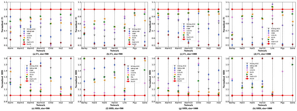
Figure 4: Normalized F1 and SHD, where the normalized value is the F1 (or SHD) value of the comparison algorithm divided by the F1 (or SHD) value of the HLCD. The larger the normalized F1 value the better, and the smaller the normalized SHD value the better.

(4) HLCD-M against PCD-by-PCD and GraN-LCS. Table 5 indicates that HLCD-M outperforms PCD-by-PCD and GraN-LCS in precision and recall across all networks. Compared to PCD-by-PCD, HLCD-M enhances precision and recall in low-dimensional networks (Alarm, Child, Insurance, and Hailfinder) by 6% to 16% and 10% to 26%, respectively, and in high-dimensional (Link, Pigs, and Gene) by 4% to 18% in precision and 2% to 22% in recall. Compared to GraN-LCS, HLCD-M consistently enhances precision by 9% to 34% and recall by 12% to 26% in low-dimensional networks, and achieves over 54% increase in precision and recall in high-dimensional networks.

Based on Table 5, HLCD-M notably reduces miss edges compared to PCD-by-PCD across all networks. Specifically, at sample sizes of 500 and 1000, HLCD-M reduces miss edges by over 12% in Alarm and Insurance networks, over 30% in Child and Gene networks, and over 5% in Hailfinder and Link networks. Regarding undirected and reverse metrics, HLCD-M exhibits fewer undirected and reverse edges in Alarm, Child, Link, Pigs, and Gene networks, and fewer reverse edges in Insurance, Barley, and Hailfinder networks. In addition, GraN-LCS requires data to conform to a Gaussian distribution and additional Gaussian noise, whereas the data generation mechanism for BN does not fulfill these criteria. As a result, GraN-LCS possesses higher structural error. Specifically, HLCD-M reduces the structural error by more than 50% in all networks except the Barley compared with GraN-LCS.

In summary, based on Fig. 4, considering both structural correctness and errors, we find the following: with a sample size of 500, HLCD achieves the highest F1 score in 14 networks and the lowest SHD count in 13 networks. With a sample size of 1000, HLCD obtains the highest F1 score in 13 networks and the lowest SHD count in 11 networks. This is attributed to HLCD’s ability to construct a more accurate local causal skeleton using Theorem 1 and to identify more precise V-structures through Theorem 2 in the skeleton orientation stage, resulting in the recognition of more precision causal orientations.

5.2.2 Time efficiency

TABLE VI: The runtime (in seconds) for HLCD and its rivals

#Sample	Network	MB-by-MB	LCS-FS	HLCD-FS	CMB	ELCS	HLCD-H	PSL	HLCD-P	PCD-by-PCD	GraN-LCS	HLCD-M
500	Alarm	0.01$\pm$0.00	0.01$\pm$0.00	0.01$\pm$0.00	0.04$\pm$0.01	0.01$\pm$0.00	0.02$\pm$0.00	0.01$\pm$0.00	0.02$\pm$0.00	0.02$\pm$0.00	9.94$\pm$0.92	0.01$\pm$0.00
	Alarm3	0.03$\pm$0.01	0.02$\pm$0.00	0.05$\pm$0.02	0.04$\pm$0.01	0.02$\pm$0.01	0.05$\pm$0.01	0.04$\pm$0.01	0.08$\pm$0.03	0.07$\pm$0.02	13.18$\pm$0.05	0.06$\pm$0.02
	Alarm5	0.07$\pm$0.02	0.03$\pm$0.01	0.11$\pm$0.04	0.06$\pm$0.00	0.04$\pm$0.00	0.11$\pm$0.03	0.09$\pm$0.03	0.12$\pm$0.03	0.22$\pm$0.05	19.23$\pm$3.28	0.14$\pm$0.03
	Alarm10	0.16$\pm$0.05	0.10$\pm$0.02	0.30$\pm$0.07	0.16$\pm$0.01	0.09$\pm$0.01	0.50$\pm$0.09	0.46$\pm$0.12	0.56$\pm$0.14	1.37$\pm$0.51	81.70$\pm$1.25	0.46$\pm$0.14
	Child	0.01$\pm$0.00	0.01$\pm$0.00	0.01$\pm$0.00	0.05$\pm$0.01	0.02$\pm$0.01	0.03$\pm$0.00	0.01$\pm$0.00	0.01$\pm$0.00	0.01$\pm$0.00	13.42$\pm$1.97	0.02$\pm$0.00
	Insurance3	0.02$\pm$0.00	0.01$\pm$0.00	0.03$\pm$0.01	0.13$\pm$0.02	0.04$\pm$0.01	0.07$\pm$0.01	0.04$\pm$0.01	0.07$\pm$0.01	0.03$\pm$0.01	19.45$\pm$1.19	0.07$\pm$0.01
	Insurance5	0.03$\pm$0.01	0.02$\pm$0.00	0.04$\pm$0.02	0.15$\pm$0.02	0.06$\pm$0.01	0.11$\pm$0.03	0.08$\pm$0.03	0.12$\pm$0.03	0.06$\pm$0.02	50.97$\pm$4.67	0.11$\pm$0.03
	Barley	0.02$\pm$0.01	0.02$\pm$0.00	0.02$\pm$0.01	21.17$\pm$17.28	2.08$\pm$1.10	1.66$\pm$0.67	10.66$\pm$4.97	1.39$\pm$0.31	17.86$\pm$4.48	23.25$\pm$3.77	2.89$\pm$0.73
	Hailfinder3	0.02$\pm$0.00	0.01$\pm$0.00	0.12$\pm$0.03	11.51$\pm$2.60	0.69$\pm$0.12	1.10$\pm$0.20	0.81$\pm$0.15	0.64$\pm$0.12	2.25$\pm$0.92	21.61$\pm$2.43	1.32$\pm$0.24
	Hailfinder5	0.04$\pm$0.01	0.02$\pm$0.00	0.30$\pm$0.10	13.13$\pm$1.36	1.77$\pm$0.88	1.96$\pm$0.33	2.36$\pm$0.33	2.26$\pm$0.43	5.49$\pm$0.61	24.19$\pm$0.94	3.69$\pm$0.54
	Hailfinder10	0.07$\pm$0.01	0.05$\pm$0.01	0.69$\pm$0.18	12.36$\pm$0.28	10.11$\pm$2.24	3.87$\pm$0.78	9.89$\pm$1.26	12.64$\pm$2.38	27.09$\pm$2.26	39.30$\pm$4.21	27.08$\pm$3.78
	Link	0.55$\pm$0.29	0.13$\pm$0.04	0.57$\pm$0.26	81.96$\pm$49.19	3.44$\pm$0.65	1.86$\pm$0.77	1.88$\pm$0.43	0.56$\pm$0.16	8.71$\pm$3.02	-	0.96$\pm$0.50
	Pigs	0.16$\pm$0.02	0.04$\pm$0.00	0.06$\pm$0.02	4.44$\pm$0.59	0.21$\pm$0.10	1.66$\pm$0.09	0.89$\pm$0.23	0.44$\pm$0.06	1.20$\pm$0.05	21.94$\pm$4.97	0.92$\pm$0.22
	Gene	0.25$\pm$0.04	0.21$\pm$0.03	1.18$\pm$0.37	0.39$\pm$0.10	0.52$\pm$0.07	0.76$\pm$0.14	2.01$\pm$0.37	2.11$\pm$0.39	4.18$\pm$0.44	-	0.90$\pm$0.13
1000	Alarm	0.01$\pm$0.00	0.01$\pm$0.00	0.01$\pm$0.00	0.03$\pm$0.00	0.01$\pm$0.00	0.02$\pm$0.01	0.02$\pm$0.00	0.02$\pm$0.00	0.02$\pm$0.00	13.00$\pm$1.32	0.01$\pm$0.00
	Alarm3	0.06$\pm$0.02	0.02$\pm$0.00	0.07$\pm$0.02	0.05$\pm$0.01	0.05$\pm$0.01	0.11$\pm$0.02	0.12$\pm$0.02	0.15$\pm$0.02	0.08$\pm$0.02	20.65$\pm$1.00	0.09$\pm$0.02
	Alarm5	0.09$\pm$0.02	0.03$\pm$0.00	0.17$\pm$0.04	0.06$\pm$0.00	0.07$\pm$0.01	0.17$\pm$0.05	0.21$\pm$0.05	0.24$\pm$0.05	0.16$\pm$0.03	27.77$\pm$2.21	0.16$\pm$0.05
	Alarm10	0.20$\pm$0.05	0.11$\pm$0.02	0.56$\pm$0.07	0.13$\pm$0.01	0.16$\pm$0.02	0.64$\pm$0.10	0.91$\pm$0.21	1.01$\pm$0.22	0.68$\pm$0.10	94.63$\pm$2.05	0.80$\pm$0.22
	Child	0.01$\pm$0.00	0.01$\pm$0.00	0.01$\pm$0.00	0.07$\pm$0.02	0.05$\pm$0.01	0.03$\pm$0.01	0.02$\pm$0.00	0.03$\pm$0.00	0.02$\pm$0.00	13.82$\pm$1.45	0.03$\pm$0.00
	Insurance3	0.03$\pm$0.01	0.02$\pm$0.00	0.03$\pm$0.01	0.22$\pm$0.03	0.05$\pm$0.01	0.07$\pm$0.01	0.04$\pm$0.01	0.07$\pm$0.01	0.04$\pm$0.01	21.08$\pm$0.99	0.09$\pm$0.02
	Insurance5	0.04$\pm$0.00	0.03$\pm$0.00	0.05$\pm$0.00	0.23$\pm$0.03	0.06$\pm$0.00	0.10$\pm$0.02	0.06$\pm$0.02	0.13$\pm$0.04	0.06$\pm$0.02	49.38$\pm$16.56	0.13$\pm$0.03
	Barley	0.01$\pm$0.00	0.02$\pm$0.00	0.03$\pm$0.00	31.98$\pm$5.55	1.36$\pm$0.14	2.88$\pm$0.39	4.08$\pm$0.26	1.55$\pm$0.16	13.45$\pm$1.57	29.54$\pm$2.95	4.28$\pm$0.61
	Hailfinder3	0.03$\pm$0.01	0.03$\pm$0.00	0.11$\pm$0.02	7.40$\pm$1.09	0.17$\pm$0.02	1.25$\pm$0.16	0.28$\pm$0.03	0.56$\pm$0.08	0.61$\pm$0.07	25.39$\pm$1.67	0.76$\pm$0.09
	Hailfinder5	0.05$\pm$0.01	0.05$\pm$0.00	0.22$\pm$0.09	8.19$\pm$1.44	0.28$\pm$0.11	2.21$\pm$0.30	0.53$\pm$0.05	1.10$\pm$0.21	1.06$\pm$0.16	30.32$\pm$1.59	1.54$\pm$0.20
	Hailfinder10	0.11$\pm$0.01	0.07$\pm$0.01	0.59$\pm$0.10	10.07$\pm$0.16	0.39$\pm$0.05	3.95$\pm$0.39	1.58$\pm$0.22	3.36$\pm$0.50	1.45$\pm$0.16	53.64$\pm$4.35	3.39$\pm$0.53
	Link	1.18$\pm$0.38	0.11$\pm$0.00	0.27$\pm$0.04	191.86$\pm$30.79	2.97$\pm$0.67	4.97$\pm$1.37	2.80$\pm$0.76	1.95$\pm$0.41	14.70$\pm$1.19	-	3.20$\pm$0.77
	Pigs	0.14$\pm$0.02	0.07$\pm$0.00	0.06$\pm$0.03	4.35$\pm$0.77	0.14$\pm$0.06	1.47$\pm$0.13	0.86$\pm$0.15	0.47$\pm$0.08	1.36$\pm$0.08	38.12$\pm$4.75	0.97$\pm$0.13
	Gene	0.26$\pm$0.04	0.42$\pm$0.07	1.14$\pm$0.27	0.70$\pm$0.15	0.61$\pm$0.07	1.19$\pm$0.26	2.37$\pm$0.68	0.10$\pm$0.02	3.37$\pm$0.72	-	1.08$\pm$0.15

TABLE VII: Results of ablation experiments for Theorem 1 and Theorem 2

#Sample	Network	Total_PC	Get_PC (↑)	Accuracy (↑)	Total_NoPC	Delete_NoPC (↑)	Accuracy (↑)	Total_V	Get_V (↑)	Accuracy (↑)	Total_NoV	Get_NoV (↑)	Accuracy (↑)
500	Alarm5	530	472.40$\pm$6.65	0.89$\pm$0.01	33695	27300.00$\pm$183.12	0.81$\pm$0.01	140	116.80$\pm$3.99	0.83$\pm$0.03	635	516.20$\pm$7.76	0.81$\pm$0.01
	Alarm10	1140	1002.00$\pm$5.08	0.88$\pm$0.00	135760	108105.80$\pm$577.72	0.80$\pm$0.00	298	240.60$\pm$1.84	0.81$\pm$0.01	1526	1245.90$\pm$16.56	0.82$\pm$0.01
	Hailfinder5	916	754.00$\pm$13.76	0.83$\pm$0.02	77484	64868.80$\pm$170.30	0.84$\pm$0.00	357	262.00$\pm$5.25	0.73$\pm$0.01	1551	1236.40+11.98	0.80+0.01
	Hailfinder10	2034	1618.60$\pm$16.49	0.80$\pm$0.01	311566	265814.00$\pm$301.27	0.85$\pm$0.00	850	610.40+9.61	0.72+0.01	3767	2981.20+27.17	0.79+0.01
	Link	2250	1778.40$\pm$0.84	0.80$\pm$0.00	521926	418718.60$\pm$1057.86	0.81$\pm$0.00	821	705.10$\pm$35.34	0.86$\pm$0.04	6986	5821.40$\pm$160.61	0.83$\pm$0.02
	Pigs	1184	1184.00$\pm$0.00	1.00$\pm$0.00	193297	189196.00$\pm$184.21	0.98$\pm$0.00	296	295.90$\pm$0.32	1.00$\pm$0.00	3229	3228.60$\pm$0.70	1.00$\pm$0.00
	Gene	1944	1933.20$\pm$2.86	0.99$\pm$0.00	639657	622343.80$\pm$472.18	0.97$\pm$0.00	269	254.90$\pm$1.97	0.95$\pm$0.01	2691	2679.10$\pm$3.35	1.00$\pm$0.00
1000	Alarm5	530	473.40$\pm$5.34	0.89$\pm$0.01	33695	28930.60$\pm$166.43	0.86$\pm$0.00	140	120.30$\pm$2.54	0.86$\pm$0.02	635	523.90$\pm$9.59	0.83$\pm$0.02
	Alarm10	1140	1002.60$\pm$8.80	0.88$\pm$0.01	135760	116155.00$\pm$454.16	0.86$\pm$0.00	298	252.10$\pm$2.38	0.85$\pm$0.01	1526	1284.20$\pm$12.97	0.84$\pm$0.01
	Hailfinder5	916	797.20$\pm$8.55	0.87$\pm$0.01	77484	64481.80$\pm$175.08	0.83$\pm$0.00	357	281.80+4.66	0.79+0.01	1551	1279.50+14.35	0.82+0.01
	Hailfinder10	2034	1728.80$\pm$14.73	0.85$\pm$0.01	311566	268080.70$\pm$225.01	0.86$\pm$0.00	850	671.50+7.41	0.79+0.01	3767	3007.20+16.98	0.80+0.00
	Link	2250	1779.00$\pm$1.05	0.80$\pm$0.00	521926	419386.40$\pm$535.96	0.81$\pm$0.00	821	773.80$\pm$15.89	0.94$\pm$0.02	6986	5838.00$\pm$98.12	0.84$\pm$0.01
	Pigs	1184	1184.00$\pm$0.00	1.00$\pm$0.00	193297	187357.80$\pm$132.39	0.97$\pm$0.00	296	296.00$\pm$0.00	1.00$\pm$0.00	3229	3229.00$\pm$0.00	1.00$\pm$0.00
	Gene	1944	1939.00$\pm$1.70	1.00$\pm$0.00	639657	620068.60$\pm$421.87	0.97$\pm$0.00	269	257.30$\pm$1.95	0.96$\pm$0.01	2691	2687.20$\pm$1.03	1.00$\pm$0.00

Table 6 illustrates the runtime performance of each algorithm. Overall, LCS-FS outperforms other algorithms in most networks, particularly excelling in Barley, Hailfinder, Pig, and Link networks. HLCD-FS shows higher efficiency compared to MB-by-MB in Link, Pigs, and Gene networks, while slightly lower efficiency in Alarm and Hailfinder networks, with comparable efficiency in other networks. HLCD-H exhibits lower time efficiency in most networks compared to ELCS, but outperforms CMB in Child, Insurance, Barley, Hailfinder, Link, and Pigs networks. Against PSL, HLCD-P shows better time efficiency in high-dimensional networks but slightly weaker efficiency in low-dimensional networks. In comparison to PCD-by-PCD, HLCD-M generally outperforms PCD-by-PCD in time efficiency, especially at a sample size of 500. Additionally, the gradient-based GraN-LCS algorithm involves extensive matrix operations, resulting in lower time efficiency, and it can only scale to high-dimensional datasets with GPU acceleration.

In a more detailed analysis, the primary time investment in local causal discovery is concentrated in the local skeleton construction stage. LCS-FS and HLCD-FS employ the mutual information-based approach for skeleton construction, making it time-saving and efficient, outperforming local causal discovery algorithms based on constraint-based skeleton construction. MB-by-MB introduces the synchronized MB learning algorithm IAMB, providing more time-efficient results than the divide-and-conquer MB learning algorithm. ELCS reduces the number of CI through N-structures, exhibiting good time efficiency compared to other constraint-based algorithms. HLCD-H and HLCD-P exhibit better time efficiency than PCD-by-PCD, as the HITON-PC and PC-simple algorithms are more effective than the MMPC algorithm. The gradient-based GraN-LCS, using deep neural network models, exhibits the lowest efficiency in all networks.

Furthermore, due to the characteristic of local causal discovery algorithms gradually expanding outward, when an algorithm misidentifies the causal direction of the target variable, it stops expanding outward to reduce time expenditure. However, this can increase the number of reverse edges, thereby reducing accuracy and recall. In other words, compared to other algorithms, HLCD is not the most time-efficient. This is because we aim to identify more correct causal directions, ensuring the learning of the correct causal structure of the target variable before ending the outward expansion. While this increases time expenditure, it reduces the number of reverse edges, thereby enhancing the precision and recall of the algorithm.

5.2.3 Ablation experiment

Finally, to visually validate the correctness of Theorems 1 and Theorems 2, we conducted ablation experiments on true graphs. Specifically, we computed the PC node set and non-PC node set for each node in the real graph, obtaining the overall counts of PC (Total_PC) and non-PC nodes (Total_NoPC) in the network. Then, applying Theorem 1, we removed the PC set and non-PC set for each node, resulting in the number of PC nodes retained (Get_PC) and non-PC nodes removed (Delete_NoPC) according to Theorem 1. Similarly, to validate Theorem 2, we tallied the number of V-structures and equivalent class structures formed by each node and its PC set in the true graph, deriving the overall counts of V-structures (Total_V) and equivalent class structures (Total_NoV) in the network. We used Theorem 2 to determine whether each V-structure and equivalent class structure was correctly identified, yielding the counts of correctly identified V-structures (Get_V) and equivalent class structures (Get_NoV). Additionally, to ensure the statistical significance of the experiments, we conducted these experiments on networks with more than 180 nodes and calculated the accuracy for each metrics.

According to Table 7, the following conclusions are drawn: At a sample size of 500, Theorem 1 removes more than 80% to 98% of redundant causal nodes in the Alarm, Hailfinder, Link, Pigs, and Gene networks, while retaining over 80% to 100% of correct causal nodes. At a sample size of 1000, Theorem 1 increases the removal rate of redundant nodes to 81% to 97%, and raises the retention rate of correct causal nodes to 80% to 100% in these networks. Regarding the identification of V-structures and equivalent class structures, at a sample size of 500, Theorem 2 correctly identifies V-structures with accuracy rates of approximately 72% to 100% and equivalent class structures with accuracy rates of approximately 79% to 100% in the mentioned networks. When the sample size reaches 1000, the accuracy of Theorem 2 in recognizing V-structures and equivalence class is further improved.

Further analysis, as the algorithm removes more redundant causal nodes, the number of correct causal nodes it removes increases as well. Similarly, as more correct V-structures are recognized, the number of correctly recognized equivalence classes decreases. Theorem 1 and Theorem 2 can synthesize and balance the two well, respectively, which is one of the reasons for the high precision and recall of the HLCD algorithm.

6 Conclusion

In this paper, we discuss the limitations of AND and OR rules in constructing exact local causal skeletons, and the problem of global causal discovery methods randomly returning incorrect local causal networks due to equivalence classes. To address the above issues, we propose a new hybrid local causal discovery algorithm (HLCD). Specifically, During the skeleton construction phase, HLCD uses maximized local scores to eliminate redundant causal skeleton structures, thereby providing a more precise causal network space. In the skeleton orientation phase, HLCD employs an innovative score-based V-structure identification approach to avoid interference caused by equivalence classes. The experimental results show that the quality of local causal discovery of HLCD is significantly better than existing methods, especially in the small sample case. In future work, we may consider a hybrid approach to improve the accuracy of MB discovery for class variables.

Zhaolong Ling received the the PhD degree in the School of of Computer and Information at the Hefei University of Technology, China, in 2020. He is a Assistant Professor with the School of Computer Science and Technology, Anhui University, China. He has published more than 10 papers in highly regarded journals, including IEEE TKDE, ACM TIST, ACM TKDD, IEEE TBD, etc. His research interests include data mining, and casual discover.

Honghui Peng received the B.S. degree from Foshan University, China, in 2022. Currently, he is working toward the MSc degree in the School of Computer Science and Technology, Anhui University, China. His research interests include feature selection, casual discovery, and data mining.

Yiwen Zhang received the Ph.D. degree in management science and engineering from the Hefei University of Technology, in 2013. He is currently a Professor with the School of Computer Science and Technology, Anhui University. Meanwhile, he is a Ph.D. advisor. His research interests include service computing, cloud computing, and big data analytics. Until now, Dr. Zhang has published more than 70 papers in some international conferences including ICSOC, ICWS and journals including IEEE TKDE, ACM TOIS, IEEE TSC, IEEE TMC, ACM TKDD, IEEE TSMC, IEEE TBD, IEEE TNNLS, IEEE TCSS, IEEE TNSE.

Peng Zhou received the B.E. degree in computer science and technology from University of Science and Technology of China in 2011, and Ph.D degree in Computer Science from Institute of Software, Chinese Academy of Sciences in 2017. He is currently an Associate Professor with the School of Computer Science and Technology, Anhui University. He has published more than 20 papers in highly regarded conferences and journals, including IEEE TNNLS, IEEE TCYB, Pattern Recognition, IJCAI, AAAI, SDM, ICDM, etc. His research interests include machine learning, data mining and artificial intelligence. More publications and codes can be found in his homepage: https://doctor-nobody.github.io/.

Xingyu Wu received the BS degree from the University of Electronic Science and Technology of China (UESTC), Chengdu, China, in 2018, and the PhD degree from University of Science and Technology of China (USTC), Hefei, China, in 2023. He is currently a postdoctoral fellow in the Department of Computing, The Hong Kong Polytechnic University. His research interests include causality-based machine learning, automatic machine learning, and large-scale pretraining model.

Kui Yu received his PhD degree in Computer Science in 2013 from the Hefei University of Technology, China. From 2013 to 2015, he was a postdoctoral fellow at the School of Computing Science of Simon Fraser University, Canada. From 2015 to 2018, He was a research fellow at the University of South Australia, Australia. He is a Professor with the School of Computer and Information, Hefei University of Technology. His main research interests include causal discovery and machine learning.

Xindong Wu received his Bachelor’s and Master’s degrees in Computer Science from the Hefei University of Technology, China, and his Ph.D. degree in Artificial Intelligence from the University of Edinburgh, Britain, in 1993. He is a Foreign Member of the Russian Academy of Engineering, and a Fellow of IEEE and the AAAS (American Association for the Advancement of Science). He is Director and Professor of the Key Laboratory of Knowledge Engineering with Big Data (the Ministry of Education of China), Hefei University of Technology, China. His research interests include big data analytics, data mining and knowledge engineering.

References

- [1] B. Huang, K. Zhang, M. Gong, and C. Glymour, “Causal discovery and forecasting in nonstationary environments with state-space models,” in International conference on machine learning. PMLR, 2019, pp. 2901–2910.
- [2] M. Prosperi, Y. Guo, M. Sperrin, J. S. Koopman, J. S. Min, X. He, S. Rich, M. Wang, I. E. Buchan, and J. Bian, “Causal inference and counterfactual prediction in machine learning for actionable healthcare,” Nature Machine Intelligence, vol. 2, no. 7, pp. 369–375, 2020.
- [3] K. Yu, X. Guo, L. Liu, J. Li, H. Wang, Z. Ling, and X. Wu, “Causality-based feature selection: Methods and evaluations,” ACM Computing Surveys (CSUR), vol. 53, no. 5, pp. 1–36, 2020.
- [4] P. Cui, Z. Shen, S. Li, L. Yao, Y. Li, Z. Chu, and J. Gao, “Causal inference meets machine learning,” in Proceedings of the 26th ACM SIGKDD International Conference on Knowledge Discovery & Data Mining, 2020, pp. 3527–3528.
- [5] C. Zhang, H. Zhang, W. Xie, N. Liu, K. Wu, and L. Chen, “Where to: Crowd-aided path selection by selective bayesian network,” IEEE Transactions on Knowledge and Data Engineering, vol. 35, no. 1, pp. 1072–1087, 2021.
- [6] M. H. Maathuis, M. Kalisch, and P. Bühlmann, “Estimating high-dimensional intervention effects from observational data,” 2009.
- [7] P. Spirtes, C. N. Glymour, R. Scheines, and D. Heckerman, Causation, prediction, and search. MIT press, 2000.
- [8] I. Tsamardinos, L. E. Brown, and C. F. Aliferis, “The max-min hill-climbing bayesian network structure learning algorithm,” Machine learning, vol. 65, pp. 31–78, 2006.
- [9] T. Gao, K. Fadnis, and M. Campbell, “Local-to-global bayesian network structure learning,” in International Conference on Machine Learning. PMLR, 2017, pp. 1193–1202.
- [10] X. Guo, K. Yu, L. Liu, P. Li, and J. Li, “Adaptive skeleton construction for accurate dag learning,” IEEE Transactions on Knowledge and Data Engineering, p. DOI 10.1109/TKDE.2023.3265015, 2023.
- [11] A. Statnikov, S. Ma, M. Henaff, N. Lytkin, E. Efstathiadis, E. R. Peskin, and C. F. Aliferis, “Ultra-scalable and efficient methods for hybrid observational and experimental local causal pathway discovery,” The Journal of Machine Learning Research, vol. 16, no. 1, pp. 3219–3267, 2015.
- [12] D. You, S. Dong, S. Niu, H. Yan, Z. Chen, S. Jin, D. Wu, and X. Wu, “Local causal structure learning for streaming features,” Information Sciences, vol. 647, p. 119502, 2023.
- [13] S. Sheng, X. Guo, K. Yu, and X. Wu, “Local causal structure learning with missing data,” Expert Systems with Applications, vol. 238, p. 121831, 2024.
- [14] J. Liang, J. Wang, G. Yu, C. Domeniconi, X. Zhang, and M. Guo, “Gradient-based local causal structure learning,” IEEE Transactions on Cybernetics, p. DOI 10.1109/TCYB.2023.3237635, 2023.
- [15] X. Wu, Y. Zhong, Z. Ling, J. Yang, L. Li, W. Sheng, and B. Jiang, “Nonlinear learning method for local causal structures,” Information Sciences, vol. 654, p. 119789, 2024.
- [16] G. Xiang, H. Wang, K. Yu, X. Guo, F. Cao, and Y. Song, “Bootstrap-based layer-wise refining for causal structure learning,” IEEE Transactions on Artificial Intelligence, p. DOI 10.1109/TAI.2023.3329786, 2023.
- [17] X. Wu, B. Jiang, Y. Zhong, and H. Chen, “Multi-target markov boundary discovery: Theory, algorithm, and application,” IEEE Transactions on Pattern Analysis and Machine Intelligence, vol. 45, no. 4, pp. 4964–4980, 2022.
- [18] X. Guo, K. Yu, L. Liu, F. Cao, and J. Li, “Causal feature selection with dual correction,” IEEE Transactions on Neural Networks and Learning Systems, 2022.
- [19] X. Wu, B. Jiang, K. Yu, H. Chen et al., “Accurate markov boundary discovery for causal feature selection,” IEEE transactions on cybernetics, vol. 50, no. 12, pp. 4983–4996, 2019.
- [20] X. Wu, B. Jiang, K. Yu, and H. Chen, “Separation and recovery markov boundary discovery and its application in eeg-based emotion recognition,” Information Sciences, vol. 571, pp. 262–278, 2021.
- [21] G. F. Cooper, “A simple constraint-based algorithm for efficiently mining observational databases for causal relationships,” Data Mining and Knowledge Discovery, vol. 1, pp. 203–224, 1997.
- [22] S. Mani and G. F. Cooper, “Causal discovery using a bayesian local causal discovery algorithm,” in MEDINFO 2004. IOS Press, 2004, pp. 731–735.
- [23] J. Yin, Y. Zhou, C. Wang, P. He, C. Zheng, and Z. Geng, “Partial orientation and local structural learning of causal networks for prediction,” in Causation and Prediction Challenge. PMLR, 2008, pp. 93–105.
- [24] C. Meek, “Causal inference and causal explanation with background knowledge,” in Proceedings of the Eleventh Conference on Uncertainty in Artificial Intelligence, 1995, pp. 403–410.
- [25] C. Wang, Y. Zhou, Q. Zhao, and Z. Geng, “Discovering and orienting the edges connected to a target variable in a dag via a sequential local learning approach,” Computational Statistics & Data Analysis, vol. 77, pp. 252–266, 2014.
- [26] T. Gao and Q. Ji, “Local causal discovery of direct causes and effects,” Advances in Neural Information Processing Systems, vol. 28, 2015.
- [27] C. F. Aliferis, I. Tsamardinos, and A. Statnikov, “Hiton: a novel markov blanket algorithm for optimal variable selection,” in AMIA annual symposium proceedings, vol. 2003. American Medical Informatics Association, 2003, pp. 21–25.
- [28] Z. Ling, K. Yu, H. Wang, L. Li, and X. Wu, “Using feature selection for local causal structure learning,” IEEE Transactions on Emerging Topics in Computational Intelligence, vol. 5, no. 4, pp. 530–540, 2020.
- [29] H. Peng, F. Long, and C. Ding, “Feature selection based on mutual information criteria of max-dependency, max-relevance, and min-redundancy,” IEEE Transactions on pattern analysis and machine intelligence, vol. 27, no. 8, pp. 1226–1238, 2005.
- [30] S. Yang, H. Wang, K. Yu, F. Cao, and X. Wu, “Towards efficient local causal structure learning,” IEEE Transactions on Big Data, vol. 8, no. 6, pp. 1592–1609, 2021.
- [31] Z. Ling, K. Yu, L. Liu, J. Li, Y. Zhang, and X. Wu, “Psl: An algorithm for partial bayesian network structure learning,” ACM Transactions on Knowledge Discovery from Data (TKDD), vol. 16, no. 5, pp. 1–25, 2022.
- [32] T. Gao and Q. Ji, “Efficient score-based markov blanket discovery,” International Journal of Approximate Reasoning, vol. 80, pp. 277–293, 2017.
- [33] D. M. Chickering, “Optimal structure identification with greedy search,” Journal of machine learning research, vol. 3, no. Nov, pp. 507–554, 2002.
- [34] N. K. Kitson, A. C. Constantinou, Z. Guo, Y. Liu, and K. Chobtham, “A survey of bayesian network structure learning,” Artificial Intelligence Review, pp. 1–94, 2023.
- [35] Z. Ling, K. Yu, Y. Zhang, L. Liu, and J. Li, “Causal learner: A toolbox for causal structure and markov blanket learning,” Pattern Recognition Letters, vol. 163, pp. 92–95, 2022.
- [36] I. Tsamardinos, C. F. Aliferis, and A. Statnikov, “Time and sample efficient discovery of markov blankets and direct causal relations,” in Proceedings of the ninth ACM SIGKDD international conference on Knowledge discovery and data mining. ACM, 2003, pp. 673–678.
- [37] I. Tsamardinos, C. F. Aliferis, A. R. Statnikov, and E. Statnikov, “Algorithms for large scale markov blanket discovery.” in FLAIRS conference, vol. 2, 2003, pp. 376–380.
- [38] J. Li, L. Liu, and T. D. Le, Practical approaches to causal relationship exploration. Springer, 2015.