A polynomial bosonic form of statistical configuration sums and the odd/even minimal excludant in integer partitions

Abstract

Inspired by the study of the minimal excludant in integer partitions by G.E. Andrews and D. Newman, we introduce a pair of new partition statistics, squrank and recrank. It is related to a polynomial bosonic form of statistical configuration sums for an integrable cellular automaton. For all nonnegative integer $n$, we prove that the partitions of $n$ on which squrank or recrank takes on a particular value, say $r$, are equinumerous with the partitions of $n$ on which the odd/even minimal exclutant takes on the corresponding value, $2r+1$ or $2r+2$.

1 Introduction

A partition of a positive integer $n$ is a finite weakly decreasing sequence of positive integers $\lambda=(\lambda_{1},\dots,\lambda_{r})$ such that $\sum_{i=1}^{r}\lambda_{i}=n$. It is sometimes written as $\lambda\vdash n$, and each $\lambda_{i}$ is called a part of $\lambda$. The integer partitions are denoted by $\mathscr{P}$, where the empty sequence for the only partition of zero (denoted by $\emptyset$) is also included as an element.

Recently, Andrews and Newman initiated studies on the minimal excludant in integer partitions and found many remarkable relations between different partition statistics [4]. They introduced the minimal excludant function ${\rm mex}_{A,a}:\mathscr{P}\rightarrow\mathbb{Z}_{>0}$ by letting ${\rm mex}_{A,a}(\lambda)$ be the smallest positive integer congruent to $a$ modulo $A$ that is not a part of $\lambda$. They also defined $p_{A,a}(n)$ to be the number of the partitions of $n$ on which ${\rm mex}_{A,a}$ takes on values congruent to $a$ modulo $2A$. This in particular implies that $p_{2,2}(n)$ is the number of the partitions of $n$ whose ‘even minimal excludant’ is not a multiple of four. They asked, at least in the author’s interpretation, a question about the existence of a different partition statistic that can reproduce the same integer sequence $\{p_{2,2}(n)\}_{n\geq 0}$ [4, p. 9, Questions II]. This question naturally arises because they have already found theorems on the existence of such partition statistics that are different from ${\rm mex}_{1,1}$ and ${\rm mex}_{3,3}$ but can reproduce the same integer sequences $\{p_{1,1}(n)\}_{n\geq 0}$ and $\{p_{3,3}(n)\}_{n\geq 0}$ [4, Theorems 2 and 3]. More specifically, they found that the relevant partition statistics are Dyson’s crank and rank [7, 3].

Motivated by this question, in this paper we introduce a pair of new partition statistics by a fairly succinct definition in combinatorics, which we call squrank and recrank. For all nonnegative integer $n$, we prove that the partitions of $n$ on which squrank or recrank takes on a particular value, say $r$, are equinumerous with the partitions of $n$ on which the odd/even minimal exclutant takes on the corresponding value, $2r+1$ or $2r+2$. This is the main result of this paper (Theorem 1). As a corollary of this theorem, the above question by Andrews and Newman is also answered.

To establish the main result, we use the fact that our new partition statistics are associated with a polynomial bosonic form of statistical configuration sums for an integrable cellular automaton [9, 13]. Let us briefly explain the relation between this bosonic form and a formula by Andrews and Newman [4], and give a comment on relevant historical backgrounds in mathematical physics. We use standard notations $(z;q)_{n}=\prod_{k=1}^{n}(1-zq^{k-1})$ for $n\geq 1$, and $(z;q)_{0}=1$. The Gaussian polynomial ${n\brack m}$ is defined by

$${n\brack m}=\begin{cases}(q;q)_{n}(q;q)_{m}^{-1}(q;q)_{n-m}^{-1}&\mbox{if }0\leq m\leq n,\\ 0&\mbox{otherwise}.\end{cases}$$ (1)

As a suggestion to solve the above open question, Andrews and Newman presented the following expression for the generating function of $p_{2,2}(n)$

$$\sum_{n\geq 0}p_{2,2}(n)q^{n}=\sum_{n\geq 0}\frac{q^{n^{2}+n}B_{n}(q)}{(q;q)_{2n+1}},$$

where $B_{n}(q)$ is a polynomial in $q$ that is written as an alternating sum of the Gaussian polynomials (See (10) in the main text). Three conjectures about this polynomial were given, for which we present two of them [4, p. 9, Questions II (1) and II (3)]:

• $B_{n}(q)$ has nonnegative coefficients.

• $B_{n}(q)$ enumerates some subset of the partitions into at most $n$ parts each $\leq n+1$.

S. Chern [5] gave a proof of the first assertion. As was mentioned therein, to verify this assertion it suffices to prove that the polynomial

$$X^{+}_{L,s}(q)={L\brack s}-{L\brack s-1},$$

has nonnegative coefficients for $1\leq s\leq L/2$. However, it was known that this polynomial takes the following statistical configuration sum form [9, 13]

$$X^{+}_{L,s}(q)=\sum_{\eta\in\mathcal{H}^{+}(L,s)}q^{E(\eta)},$$

where $\mathcal{H}^{+}(L,s)$ is a subset of the bit sequences of $s$ ones and $L-s$ zeros, and $E(\eta)$ is an energy attributed to bit sequences $\eta$ (See (20) in the main text). From this viewpoint, the non-negativity of the coefficients of the polynomial is obvious. The above expression of this polynomial as a subtraction of two Gaussian polynomials, or such expressions for more general polynomials or series with nonnegative coefficients by formulae including subtractions, are sometimes called bosonic forms. This terminology was used in the study of the formulae for conformal field theory characters and branching functions [12], and such formulae have their origin in the study of exactly solvable lattice models in $2D$ statistical mechanics [2].

This relation enables us to verify the second assertion of the above conjecture for $B_{n}(q)$, by introducing a partition theoretic function to specify the unidentified subset of the set of restricted partitions. This function, denoted by $\mathcal{E}_{1}$, has its origin in algebraic combinatorics or more precisely in the theory of crystals [8], and plays an essential role in the proof of the main theorem. To obtain a useful form for this function, we use the notion of the path-encoding of the box-ball system in a recent study on the integrable cellular automaton [6].

The remainder of this paper is organized as follows. In Sect. 2, after reviewing necessary notions about integer partitions and Ferrers diagrams, we present the definition of our new partition statistics through a combinatorial procedure and state the main theorem. Everything what follows are for the proof of this theorem. In Sect. 3, we derive formulae for the generating functions of a pair of mex-related functions and find that the polynomial bosonic form appears there. In Sect. 4, we prove that the bosonic form can be expressed as a statistical configuration sum over the set of bit sequences with a restriction. In Sect. 5 and Sect. 6, we define an energy preserving bijection between restricted partitions and bit sequences, and also define a similar bijection between partitions and pairs of partitions. In Sect. 7 we give a proof of the main theorem, and finally in Sect. 8 we present concluding remarks.

2 Preliminaries and the main result

Throughout this paper, we identify partitions with the corresponding Ferrers diagrams, in which dots are replaced by unit squares called cells. The cell in row $i$ and column $j$ has coordinate $(i,j)$, as in a matrix. We sometimes use the following notation for a non empty partition $\lambda$ [10]. Suppose that the main diagonal of the diagram of $\lambda$ consists of $d$ cells $(i,i)\,(1\leq i\leq d)$. Such $d=d(\lambda)$ is called the side of the Durfee square of $\lambda$ [1]. Let $x_{i}$ be the number of cells in the $i$th row of $\lambda$ to the right of $(i,i)$, and let $y_{i}$ be the number of cells in the $i$th column of $\lambda$ below $(i,i)$, for $1\leq i\leq d$. Then we define the Frobenius representation of $\lambda$ to be $F(\lambda)=(x_{1},\dots,x_{d}\mid y_{1},\dots,y_{d})$. See Fig. 1 for an example.

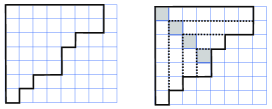
Figure 1: (left) The Ferrers diagram for partition $\lambda=(7,7,5,4,4,2,1).$; (right) Its decomposition into the hooks for recognizing its Frobenius representation $F(\lambda)=(6,5,2,0\mid 6,4,2,1)$.

A rim hook (also called a border strip) is a skew diagram if it is edgewise connected and contains no $2\times 2$ block of cells [11]. The number of all cells contained in a rim hook is called its length. By generalizing the corresponding notions for a hook [11], we define the arm length of a rim hook to be one less than the number of columns it occupies, and the leg length of a rim hook to be one less than the number of rows it occupies. The rim of a Ferrers diagram $\lambda$ is defined to be the rim hook that consists of all the cells along the south-east border of $\lambda$. More precisely, if $F(\lambda)=(x_{1},\dots,x_{d}\mid y_{1},\dots,y_{d})$, then the rim of $\lambda$ is defined by the skew shape $\lambda/\nu$ where $\nu$ is the partition uniquely determined by $F(\nu)=(x_{2},\dots,x_{d}\mid y_{2},\dots,y_{d})$.

Now we introduce the pair of partition statistics or maps from $\mathscr{P}$ to $\mathbb{Z}_{\geq 0}$, tentatively denoted by $f^{(a)}\,(a=0,1)$, by the following procedure. Given $\lambda\in\mathscr{P}$;

1. Let $D_{0}(\lambda)$ be the largest square inside $\lambda$, and let $D_{1}(\lambda)$ be the largest rectangle inside $\lambda$ whose horizontal side is larger than whose vertical side by one. Let $n_{a}=n_{a}(\lambda)$ denote the vertical side of $D_{a}(\lambda)$, and let $A_{a}(\lambda)$ denote the sub-diagram of $\lambda$ that consists of the cells inside the first $n_{a}$ rows but not in $D_{a}(\lambda)$ .

2. From diagram $A_{a}(\lambda)$, strip away the longest of the rightmost rim hooks with arm length $n_{a}+a$ lying along the rim of the diagram. Repeat the same procedure until the remaining diagram has less than $n_{a}+a+1$ columns, and let $R_{a}(\lambda)$ denote the residual diagram.

3. Let $F(R_{a}(\lambda))=(x_{1},\dots,x_{d}\mid y_{1},\dots,y_{d})$. Set $y_{0}=n_{a},x_{d+1}=-1$ and define

   $$f^{(a)}(\lambda):=\max_{0\leq i\leq d}(y_{i}-x_{i+1})-1.$$

The author proposes the following:

Definition 1.

For partitions $\lambda$, we define

1. ${\rm squrank}(\lambda)=f^{(0)}(\lambda)$,

2. ${\rm recrank}(\lambda)=f^{(1)}(\lambda)$.

In what follows, we call $D_{0}(\lambda)$ (resp. $D_{1}(\lambda)$) the Durfee square (resp. Durfee rectangle) of the partition $\lambda$.

Example 1.

Let $\lambda=(19,16,9,2,1)$. Then we have $n_{0}=3,D_{0}(\lambda)=(3,3,3)$ and $A_{0}(\lambda)=(16,13,6)$. After stripping away the rim hooks with arm length 3 from $A_{0}(\lambda)$, one has $R_{0}(\lambda)=(1,1)$. Then we find $F(R_{0}(\lambda))=(0\mid 1)$ and hence ${\rm squrank}(\lambda)=\max(y_{0}-x_{1},y_{1}-x_{2})-1=\max(3-0,1-(-1))-1=2$. See Fig 2.

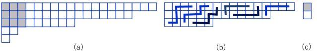
Figure 2: (a) The diagram of $\lambda$ and its Durfee square $D_{0}(\lambda)$ (shaded). (b) The rim hooks with arm length 3 that will be stripped away from the sub-diagram $A_{0}(\lambda)$. (c) The residual diagram $R_{0}(\lambda)$ and its diagonal node (shaded).

Example 2.

Let $\lambda=(19,16,9,2,1)$. Then we have $n_{1}=3,D_{1}(\lambda)=(4,4,4)$ and $A_{1}(\lambda)=(15,12,5)$. After stripping away the rim hooks with arm length 4 from $A_{1}(\lambda)$, one has $R_{1}(\lambda)=(3,3)$. Then we find $F(R_{1}(\lambda))=(2,1\mid 1,0)$ and hence ${\rm recrank}(\lambda)=\max(y_{0}-x_{1},y_{1}-x_{2},y_{2}-x_{3})-1=\max(3-2,1-1,0-(-1))-1=0$. See Fig 3.

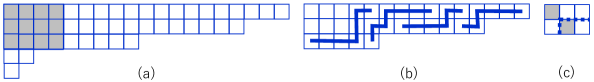
Figure 3: (a) The diagram of $\lambda$ and its Durfee rectangle $D_{1}(\lambda)$ (shaded). (b) The rim hooks with arm length 4 that will be stripped away from the sub-diagram $A_{1}(\lambda)$. (c) The residual diagram $R_{1}(\lambda)$ and its diagonal nodes (shaded), and its decomposition into the hooks.

As we introduced in Sect. 1, ${\rm mex}_{A,a}(\lambda)$ is the smallest positive integer congruent to $a$ modulo $A$ that is not a part of $\lambda$. In particular, ${\rm mex}_{2,1}(\lambda)$ (resp. ${\rm mex}_{2,2}(\lambda)$) is the smallest positive odd (resp. even) number that is not a part of $\lambda$. For all $n,r\in\mathbb{Z}_{\geq 0}$, we define

$$p^{(r)}_{2,1}(n) =\#\{\lambda\vdash n\mid{\rm mex}_{2,1}(\lambda)=2r+1\},$$ (2)

$$p^{(r)}_{2,2}(n) =\#\{\lambda\vdash n\mid{\rm mex}_{2,2}(\lambda)=2r+2\},$$ (3)

where $\#$ denotes cardinality. Here we let $p^{(r)}_{2,1}(0)=p^{(r)}_{2,2}(0)=\delta_{r,0}$ since for the only partition $\lambda=\emptyset$ of $n=0$ we have ${\rm mex}_{2,1}(\lambda)=1$ and ${\rm mex}_{2,2}(\lambda)=2$. The following is the main result of this paper.

Theorem 1.

1. $p^{(r)}_{2,1}(n)$ equals the number of partitions $\lambda$ of $n$ with ${\rm squrank}(\lambda)=r$.

2. $p^{(r)}_{2,2}(n)$ equals the number of partitions $\lambda$ of $n$ with ${\rm recrank}(\lambda)=r$.

Example 3.

Let $n=8$. Then, item 1 (resp. item 2) of Theorem 1 is shown in Table 1 (resp. Table 2 ). In this example, we use the multiplicity notation $\mu_{1}^{m_{1}}\mu_{2}^{m_{2}}\dots\mu_{\ell}^{m_{\ell}}$ to represent a partition in which $m_{i}$ denotes the multiplicity of the part $\mu_{i}$ (which is omitted when $m_{i}=1$) and $\mu_{1}>\mu_{2}>\dots>\mu_{\ell}$.

Let $p_{2,2}(n)=\sum_{m\geq 0}p^{(2m)}_{2,2}(n)$, which equals the number of partitions $\lambda$ of $n$, where

$${\rm mex}_{2,2}(\lambda)\equiv 2\pmod{4}.$$ (4)

As a direct result of the above theorem, we have:

Corollary 2.

$p_{2,2}(n)$ equals the number of partitions of $n$ with even recrank.

This is an answer to the problem by Andrews-Newman [4, p. 9, Question II].

Table 1: Comparison between squrank and ${\rm mex}_{2,1}$ for the partitions of 8

	squrank			${\rm mex}_{2,1}$
Partition	0	1	2	1	3	5
$1^{8}$		✓			✓
$21^{6}$	✓				✓
$2^{2}1^{4}$			✓		✓
$2^{3}1^{2}$			✓		✓
$2^{4}$			✓	✓
$31^{5}$		✓				✓
$321^{3}$		✓				✓
$32^{2}1$		✓				✓
$3^{2}1^{2}$		✓				✓
$3^{2}2$		✓		✓
$41^{4}$	✓				✓
$421^{2}$	✓				✓
$42^{2}$	✓			✓
$431$		✓				✓
$4^{2}$	✓			✓
$51^{3}$		✓			✓
$521$			✓		✓
$53$			✓	✓
$61^{2}$	✓				✓
$62$		✓		✓
$71$		✓			✓
$8$	✓			✓
Total	7	10	5	7	10	5

Table 2: Comparison between recrank and ${\rm mex}_{2,2}$ for the partitions of 8

	recrank			${\rm mex}_{2,2}$
Partition	0	1	2	2	4	6
$1^{8}$	✓			✓
$21^{6}$		✓			✓
$2^{2}1^{4}$		✓			✓
$2^{3}1^{2}$		✓			✓
$2^{4}$		✓			✓
$31^{5}$	✓			✓
$321^{3}$	✓				✓
$32^{2}1$	✓				✓
$3^{2}1^{2}$			✓	✓
$3^{2}2$			✓		✓
$41^{4}$	✓			✓
$421^{2}$	✓					✓
$42^{2}$	✓					✓
$431$		✓		✓
$4^{2}$		✓		✓
$51^{3}$		✓		✓
$521$		✓			✓
$53$	✓			✓
$61^{2}$	✓			✓
$62$	✓				✓
$71$	✓			✓
$8$		✓		✓
Total	11	9	2	11	9	2

3 Generating functions

In this section we establish the following formulae for the generating functions of the mex-related functions.

Proposition 3.

The following identities hold:

$$\sum_{n\geq 0}p^{(r)}_{2,1}(n)q^{n} =\sum_{n\geq 0}\frac{q^{n^{2}}Z_{2n,n}^{(r)}(q)}{(q;q)_{2n}},$$ (5)

$$\sum_{n\geq 0}p^{(r)}_{2,2}(n)q^{n} =\sum_{n\geq 0}\frac{q^{n^{2}+n}Z_{2n+1,n}^{(r)}(q)}{(q;q)_{2n+1}},$$ (6)

where

$$Z_{2n+a,n}^{(r)}(q)={2n+a\brack n-r}-{2n+a\brack n-r-1}.$$ (7)

Proof.

First we prove (5). Its right hand side can be written as

$$\sum_{n\geq 0}\frac{q^{n^{2}}Z_{2n,n}^{(r)}(q)}{(q;q)_{2n}}=\sum_{n\geq r}\frac{q^{n^{2}}}{(q;q)_{2n}}{2n\brack n-r}\\ -\,(\quad``r\rightarrow r+1"\quad),$$

where we let the second term be obtained from the first term by replacing $r$ by $r+1$. The first term can be written as

$$\sum_{n\geq r}\frac{q^{n^{2}}}{(q;q)_{2n}}{2n\brack n-r} =\sum_{n\geq r}\frac{q^{n^{2}}}{(q;q)_{n-r}(q;q)_{n+r}}$$

$$=\sum_{n\geq 0}\frac{q^{(n+r)^{2}}}{(q;q)_{n}(q;q)_{n+2r}}$$

$$=q^{r^{2}}\sum_{n\geq 0}\frac{q^{n(n+2r)}}{(q;q)_{n}(q;q)_{n+2r}}$$

$$=\frac{q^{r^{2}}}{(q;q)_{\infty}}.$$

In the last line we used $(q;q)_{n+2r}=(q;q)_{2r}(q^{2r+1};q)_{n}$ and the Cauchy formula [1, (2.2.8)]

$$\sum_{n\geq 0}\frac{q^{n^{2}-n}z^{n}}{(q;q)_{n}(z;q)_{n}}=\frac{1}{(z;q)_{\infty}},$$ (8)

with $z=q^{2r+1}$. Therefore

$$\sum_{n\geq 0}\frac{q^{n^{2}}Z_{2n,n}^{(r)}(q)}{(q;q)_{2n}} =\frac{q^{r^{2}}-q^{(r+1)^{2}}}{(q;q)_{\infty}}$$

$$=\frac{q^{r^{2}}(1-q^{2r+1})}{(q;q)_{\infty}}$$

$$=\frac{q^{r^{2}}}{\prod_{m=1,m\neq 2r+1}^{\infty}(1-q^{m})}.$$

Since $r^{2}=1+3+\dots+(2r-1)$, one finds that this expression is clearly the generating function for $p^{(r)}_{2,1}(n)$.

Next we prove (6). Its right hand side can be written as

$$\sum_{n\geq 0}\frac{q^{n^{2}+n}Z_{2n+1,n}^{(r)}(q)}{(q;q)_{2n+1}}=\sum_{n\geq r}\frac{q^{n^{2}+n}}{(q;q)_{2n+1}}{2n+1\brack n-r}\\ -\,(\quad``r\rightarrow r+1"\quad),$$

where we let the second term be obtained from the first term by replacing $r$ by $r+1$. The first term can be written as

$$\sum_{n\geq r}\frac{q^{n^{2}+n}}{(q;q)_{2n+1}}{2n+1\brack n-r} =\sum_{n\geq r}\frac{q^{n^{2}+n}}{(q;q)_{n-r}(q;q)_{n+r+1}}$$

$$=\sum_{n\geq 0}\frac{q^{(n+r)^{2}+(n+r)}}{(q;q)_{n}(q;q)_{n+2r+1}}$$

$$=q^{r^{2}+r}\sum_{n\geq 0}\frac{q^{n(n+2r+1)}}{(q;q)_{n}(q;q)_{n+2r+1}}$$

$$=\frac{q^{r(r+1)}}{(q;q)_{\infty}}.$$

In the last line we used $(q;q)_{n+2r+1}=(q;q)_{2r+1}(q^{2r+2};q)_{n}$ and the Cauchy formula (8) with $z=q^{2r+2}$. Therefore

$$\sum_{n\geq 0}\frac{q^{n^{2}+n}Z_{2n+1,n}^{(r)}(q)}{(q;q)_{2n+1}} =\frac{q^{r(r+1)}-q^{(r+1)(r+2)}}{(q;q)_{\infty}}$$

$$=\frac{q^{r(r+1)}(1-q^{2(r+1)})}{(q;q)_{\infty}}$$

$$=\frac{q^{r(r+1)}}{\prod_{m=1,m\neq 2(r+1)}^{\infty}(1-q^{m})}.$$

Since $r(r+1)=2+4+\dots+2r$, one finds that this expression is clearly the generating function for $p^{(r)}_{2,2}(n)$. ∎

Remark 1.

By summing both sides of (6) over even $r$’s, we obtain

$$\sum_{n\geq 0}p_{2,2}(n)q^{n}=\sum_{n\geq 0}\frac{q^{n^{2}+n}B_{n}(q)}{(q;q)_{2n+1}},$$ (9)

where

$$B_{n}(q)=\sum_{r=0}^{n}(-1)^{r}{2n+1\brack n-r},$$ (10)

which we have already mentioned in §1. This expression for the generating function of $p_{2,2}(n)$ was first derived through a different argument by Andrews and Newman [4].

4 A polynomial bosonic form for statistical configuration sums

In this section we present the formulae for the statistical configuration sums associated with an integrable cellular automaton which the author studied some time ago [9, 13], with an argument for proving them being supplied. Part of the following results are also presented in Japanese [14].

4.1 A linear recursion relation associated with the Gaussian polynomials

We seek a family of polynomials $G_{L,s}(q)$ satisfying the recursion relation

$$G_{L,s}(q)=G_{L-1,s}(q)+\sum_{k=1}^{s}q^{L-k}G_{L-k-1,s-k}(q),$$ (11)

for $s<L$.

Proposition 4.

Suppose that the boundary condition

$$G_{L,0}(q)=G_{L,L}(q)=1,$$ (12)

is satisfied. Then the recursion relation (11) with this boundary condition determines a unique solution $G_{L,s}(q)=:X_{L,s}(q)$ for every $0\leq s\leq L$. This polynomial has nonnegative coefficients.

Proof.

If $L-s=0$ then it is a monomial $1$ by the boundary condition, and by increasing the difference $L-s$ one by one from this case, it is successively determined by the recursion relation (11). This polynomial clearly has nonnegative coefficients by definition. ∎

Proposition 5.

Suppose $0\leq s\leq\lceil L/2\rceil$, and that the boundary conditions

$$G_{L,0}(q)=1,\quad G_{2s-1,s}(q)=0,$$ (13)

are satisfied. Then the recursion relation (11) with these boundary conditions determines a unique solution $G_{L,s}(q)=:X^{+}_{L,s}(q)$ for every $L\geq 0$ and $0\leq s\leq\lceil L/2\rceil$. This polynomial has nonnegative coefficients.

Proof.

We prove it by induction on $s$ and $L$. First we suppose $s=0$, then by the boundary condition (13) $X^{+}_{L,0}(q)$ is a polynomial with nonnegative coefficients (the monomial $1$) for every $L\geq 0$.

Next we suppose $s>0$, and for every fixed $\sigma<s$ suppose all $X^{+}_{\Lambda,\sigma}(q)$ have already been determined as polynomials with nonnegative coefficients for every $\Lambda\geq 2\sigma$.

1. Suppose $L=2s$. Then by the recursion relation (11) we have

   $$X^{+}_{2s,s}(q)=X^{+}_{2s-1,s}(q)+\sum_{k=1}^{s}q^{2s-k}X^{+}_{2s-k-1,s-k}(q),$$

   where we see that the first term in its right hand side equals $0$ by the boundary condition (13), and the second term is a summation over already determined polynomials with nonnegative coefficients. Therefore, its left hand side is also uniquely determined as a polynomial with nonnegative coefficients.

2. Suppose $L>2s$, and for every fixed $\Lambda<L$ suppose all $X^{+}_{\Lambda,s}(q)$ have already been determined as polynomials with nonnegative coefficients. Then by the recursion relation (11) we have

   $$X^{+}_{L,s}(q)=X^{+}_{L-1,s}(q)+\sum_{k=1}^{s}q^{L-k}X^{+}_{L-k-1,s-k}(q),$$

   where we see that its right hand side is a summation over already determined polynomials with nonnegative coefficients. Therefore, its left hand side is also uniquely determined as a polynomial with nonnegative coefficients.

∎

Here we summarize the definition of the above polynomials.

Definition 2.

Let $X_{L,s}(q)$ and $X^{+}_{L,s}(q)$ denote the pair of polynomials with nonnegative coefficients that are determined by;

1. Recursion relation (11) with boundary condition (12) for $X_{L,s}(q)$.

2. Recursion relation (11) with boundary condition (13) for $X^{+}_{L,s}(q)$.

These polynomials can be expressed by using Gaussian polynomials (1).

Proposition 6.

These polynomials take the following forms

$$X_{L,s}(q) ={L\brack s},$$ (14)

$$X^{+}_{L,s}(q) ={L\brack s}-{L\brack s-1}.$$ (15)

Proof.

The Gaussian polynomials satisfy the following identities [1]:

$${L\brack s} ={L\brack L-s},$$ (16)

$${L\brack s} ={L-1\brack s}+q^{L-s}{L-1\brack s-1},$$ (17)

$${L\brack s} =q^{s}{L-1\brack s}+{L-1\brack s-1}.$$ (18)

First we prove (14). By definition the Gaussian polynomials satisfy the boundary condition (12). For the identity (17), we substitute the second term of its right hand side by the left hand side of (18) but with $L,s$ replaced by $L-1,s-1$ to obtain a new identity. In the same way, we repeat substituting the rightmost term of their right hand side by the left hand side of (18) but with $L,s$ replaced by $L-k,s-k$, for $k=2,\dots,s-1$. As a result, we obtain the recursion relation (11). Since $X_{L,s}(q)$ is uniquely determined by the boundary condition and the recursion relation, we get the expression (14).

Next we prove (15). Because of the above result and the linearity of the recursion relation (11), the right hand side of (15) must satisfy the same recursion relation. In addition, by the definition of Gaussian polynomial and the identity (16), we see that the right hand side of (15) satisfies the boundary condition (13). Since $X^{+}_{L,s}(q)$ is also uniquely determined by the boundary condition and the recursion relation, we get the expression (15). ∎

Corollary 7.

1. $Z_{2n+a,n}^{(r)}(q)$ in (7) has nonnegative coefficients.

2. $B_{n}(q)$ in (10) has nonnegative coefficients.

The latter is an answer to the problem by Andrews-Newman [4, p. 9, Question II (1)].

4.2 Canonical partition functions: statistical configuration sums over bit sequences

We consider the set of all bit sequences that consists of $L-s$ zeros and $s$ ones. More explicitly we define

$$\mathcal{H}(L,s)=\{\eta\in\{0,1\}^{L}\,\mid\,|\eta|=s\},$$ (19)

where for $\eta=(\eta_{1},\dots,\eta_{L})\in\{0,1\}^{L}$ we let $|\eta|=\sum_{1\leq i\leq L}\eta_{i}$. In what follows, we sometimes write $(\eta_{1},\dots,\eta_{L})$ as $\eta_{1}\dots\eta_{L}$.

Let $H$ denote the function from $\{0,1\}^{2}$ to $\{0,1\}$ that is given by $H(0,1)=1,H(0,0)=H(1,0)=H(1,1)=0$. For bit sequences $\eta\in\mathcal{H}(L,s)$, we define their energy by

$$E(\eta)=\sum_{1\leq j\leq L-1}jH(\eta_{j},\eta_{j+1}).$$ (20)

We define the generating function enumerating the bit sequences with the energy as

$$Z_{L,s}(q)=\sum_{\eta\in\mathcal{H}(L,s)}q^{E(\eta)}.$$ (21)

Borrowing a terminology from statistical mechanics, we call this generating function a partition function.

Example 4.

Let $L=5,s=2$. The ten elements of $\mathcal{H}(5,2)$ are $11000\,(E=0)$, $01100,\,(E=1)$, $00110,10100\,(E=2)$, $00011,10010\,(E=3)$, $01010,10001\,(E=4)$, $01001\,(E=5)$, and $00101\,(E=6)$. Therefore we have $Z_{5,2}(q)=1+q+2q^{2}+2q^{3}+2q^{4}+q^{5}+q^{6}$.

Proposition 8.

$$Z_{L,s}(q)={L\brack s}.\\$$ (22)

Proof.

By Proposition 6, it suffices to show that $Z_{L,s}(q)=X_{L,s}(q)$. The only bit sequence belonging to $\mathcal{H}(L,L)$ is $(1,\dots,1)$, and that of $\mathcal{H}(L,0)$ is $(0,\dots,0)$. These bit sequences have zero energy. So, $Z_{L,s}(q)$ satisfies the boundary condition (12) and the remaining task for us is to verify the recursion relation (11).

By classifying the elements of $\mathcal{H}(L,s)$ by the positions $L-k$ of the last zero, we have

$$\mathcal{H}(L,s) =\coprod_{k=0}^{s}\mathcal{H}_{(k)}(L,s),$$

$$\mathcal{H}_{(k)}(L,s) =\{\eta\in\mathcal{H}(L,s)\,\mid\,\max\{\alpha\,\mid\,\eta_{\alpha}=0\}=L-k\}.$$

According to this disjoint union, the partition function takes the form

$$Z_{L,s}(q)=\sum_{\eta\in\mathcal{H}_{(0)}(L,s)}q^{E(\eta)}+\sum_{k=1}^{s}\sum_{\eta\in\mathcal{H}_{(k)}(L,s)}q^{E(\eta)}.$$

In the first term of the right hand side, we have $E(\eta)=\sum_{1\leq j\leq L-2}jH(\eta_{j},\eta_{j+1})$, because for every $\eta\in\mathcal{H}_{(0)}(L,s)$ we have $H(\eta_{L-1},\eta_{L})=0$. In addition, we have $\sum_{1\leq i\leq L-1}\eta_{i}=s$. This implies that the procedure of removing the last digit $0$ induces an energy preserving bijection from $\mathcal{H}_{(0)}(L,s)$ to $\mathcal{H}(L-1,s)$. Therefore, this first term equals to the first term of the right hand side of (11). In the second term of the right hand side, for each $k$, we have $E(\eta)=L-k+\sum_{1\leq j\leq L-k-1}jH(\eta_{j},\eta_{j+1})$, because for every $\eta\in\mathcal{H}_{(k)}(L,s)$ we have $H(\eta_{L-k+j},\eta_{L-k+j+1})=\delta_{j,0}$ for $0\leq j\leq k-1$. In addition, we have $\sum_{1\leq i\leq L-k-1}\eta_{i}=s-k$. This implies that the procedure of removing the last $k+1$ digits $01\dots 1$ induces a bijection from $\mathcal{H}_{(k)}(L,s)$ to $\mathcal{H}(L-1-k,s-k)$ that reduces the value of the energy by $L-k$. Therefore, this second term as a whole equals to the second term of the right hand side of (11). ∎

For $\eta\in\mathcal{H}(L,s)$ let $S(\eta)=(S_{i}(\eta))_{0\leq i\leq L}$ be its path-encoding [6] that is defined as

$$S_{0}(\eta) =0,$$

$$\quad S_{i}(\eta) =S_{i-1}(\eta)+1-2\eta_{i}\,(1\leq i\leq L).$$ (23)

See Fig 4 for an example. In what follows we call $S(\eta)$ the path for the bit sequence $\eta$.

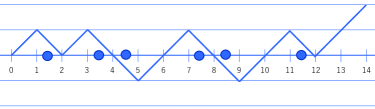
Figure 4: A graphical representation of the path $S(\eta)$ for $\eta=01011001100100$ by line segments. We put a mark $\bullet$ between coordinate $i-1$ and $i$ if $\eta_{i}=1$.

Let $\varepsilon_{1}(\eta)$ be the absolute value of the minimum of the path $S(\eta)$, i.e.

$$\varepsilon_{1}(\eta):=-\min_{0\leq i\leq L}S_{i}(\eta),$$ (24)

by which we also define the function $\varepsilon_{1}:\mathcal{H}(L,s)\rightarrow[0,s].$ By classifying the elements of $\mathcal{H}(L,s)$ by their $\varepsilon_{1}$-values, we have

$$\mathcal{H}(L,s) =\coprod_{r=0}^{s}\mathcal{H}^{(r)}(L,s),$$ (25)

$$\mathcal{H}^{(r)}(L,s) =\{\eta\mid\varepsilon_{1}(\eta)=r\}.$$

Proposition 9.

For every integer $L\geq 2$, and for every pair of integers $r,s$ satisfying the conditions $0\leq s\leq\lfloor L/2\rfloor-1,0\leq r\leq s$, there is an energy preserving bijection between $\mathcal{H}^{(r)}(L,s)$ and $\mathcal{H}^{(r+1)}(L,s+1)$ with respect to the energy (20).

Proof.

We construct the bijection explicitly. See Fig 5 for an example.

First we construct the map from $\mathcal{H}^{(r)}(L,s)$ to $\mathcal{H}^{(r+1)}(L,s+1)$, denoted by $\tilde{f}_{1}$, as follows. For all $\eta\in\mathcal{H}^{(r)}(L,s)$, we see that if $S_{i}(\eta)=-r$ then $i\leq L-2$ because we have $S_{L}(\eta)=L-2s\geq 2$, and hence $S_{L-1}(\eta)\geq 1$.

• If $\max\{i\mid S_{i}(\eta)=-r\}=0$, then $r=0$. In this case we have $(\eta_{1},\eta_{2})=(0,0)$. Replace it by $(1,0)$.

• If $\max\{i\mid S_{i}(\eta)=-r\}>0$, then we have $(\eta_{i},\eta_{i+1},\eta_{i+2})=(1,0,0)$. Replace it by $(1,1,0)$.

By this procedure, whereas the number of $1$’s becomes $s+1$ but the energy of the bit sequence does not change. Although the values of $S_{j}$ for $j>i$ decrease by $2$, they are greater than or equal to $-r-1$, and in particular we have $S_{i+1}(\tilde{f}_{1}\eta)=-r-1$. On the other hand, the values of $S_{j}$ for $j\leq i$ do not change, and hence are greater than or equal to $-r$.

Next we construct the map from $\mathcal{H}^{(r+1)}(L,s+1)$ to $\mathcal{H}^{(r)}(L,s)$, denoted by $\tilde{e}_{1}$, as follows. For all $\eta\in\mathcal{H}^{(r+1)}(L,s+1)$, we see that if $S_{i}(\eta)=-r-1$ then $1\leq i\leq L-1$, because we have $S_{L}(\eta)=L-2s-2\geq 0$, and $S_{0}(\eta)=0$.

• If $\min\{i\mid S_{i}(\eta)=-r-1\}=1$, then $r=0$. In this case we have $(\eta_{1},\eta_{2})=(1,0)$. Replace it by $(0,0)$.

• If $\min\{i\mid S_{i}(\eta)=-r-1\}>1$, then we have $(\eta_{i-1},\eta_{i},\eta_{i+1})=(1,1,0)$. Replace it by $(1,0,0)$.

By this procedure, whereas the number of $1$’s becomes $s$ but the energy of the bit sequence does not change. Since the values of $S_{j}$ for $j\geq i$ increase by $2$, they are greater than or equal to $-r+1$. On the other hand, the values of $S_{j}$ for $j<i$ do not change, and hence are greater than or equal to $-r$, and in particular we have $S_{i-1}(\tilde{e}_{1}\eta)=-r$.

It is also easy to see that the maps $\tilde{f}_{1}$ and $\tilde{e}_{1}$ are inverse to each other . ∎

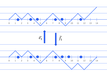
Figure 5: A graphical representation of maps $\tilde{f}_{1}$ and $\tilde{e}_{1}$. We have $\tilde{f}_{1}(01011001100100)=01011001110100\in\mathcal{H}^{(2)}(14,7)$ and $\tilde{e}_{1}(01011001110100)=01011001100100\in\mathcal{H}^{(1)}(14,6)$. The values of the energy coincide as $H(01011001100100)=H(01011001110100)=1+3+7+11=22$.

Remark 2.

The notation $\tilde{f}_{1},\tilde{e}_{1}$ for the maps in the proof of Proposition 9 is so chosen as to coincide with the notation for the Kashiwara operators in the theory of affine crystals. The notation $\varepsilon_{1}$ for the map defined in (24) is also taken from this theory. From this point of view, the set of bit sequences $\mathcal{H}(L,s)$ is regarded as a subset of $B^{\otimes L}$, where $B=\{0,1\}$ is a classical crystal. The energy (20) for bit sequences is used to interpret the sequences as elements of an affine crystal. The function $H$ (but the sign has been changed) is called an energy function [8].

According to (25), we define the partition function with fixed $\varepsilon_{1}$-values by

$$Z_{L,s}^{(r)}(q)=\sum_{\eta\in\mathcal{H}^{(r)}(L,s)}q^{E(\eta)}.$$ (26)

We show that it is consistent with a notation in (7).

Proposition 10.

$$Z_{L,s}^{(r)}(q)={L\brack s-r}-{L\brack s-r-1}.$$ (27)

Proof.

By Proposition 9, we have $Z_{L,s}^{(r)}(q)=Z_{L,s-r}^{(0)}(q)$ for $1\leq r\leq s$. Thus it suffices to establish this formula in the case of $r=0$. Then by Proposition 6, it suffices to show that $Z^{(0)}_{L,s}(q)=X^{+}_{L,s}(q)$. The only bit sequence belonging to $\mathcal{H}^{(0)}(L,0)$ is $(0,\dots,0)$, which has zero energy. On the other hand, we have $\mathcal{H}^{(0)}(2s-1,s)=\emptyset$, because the condition $S_{2s-1}(\eta)=-1$ holds for every $\eta\in\mathcal{H}(2s-1,s)$. So, $Z^{(0)}_{L,s}(q)$ satisfies the boundary condition (13) and the remaining task for us is to verify the recursion relation (11).

In what follows, let $\mathcal{H}^{+}(L,s)=\mathcal{H}^{(0)}(L,s)$. By classifying the elements of $\mathcal{H}^{+}(L,s)$ by the positions $L-k$ of the last zero, we have

$$\mathcal{H}^{+}(L,s) =\coprod_{k=0}^{s}\mathcal{H}^{+}_{(k)}(L,s),$$

$$\mathcal{H}^{+}_{(k)}(L,s) =\{\eta\in\mathcal{H}^{+}(L,s)\mid\max\{\alpha\mid\eta_{\alpha}=0\}=L-k\}.$$

According to this disjoint union, the partition function takes the form

$$Z^{(0)}_{L,s}(q)=\sum_{\eta\in\mathcal{H}^{+}_{(0)}(L,s)}q^{E(\eta)}+\sum_{k=1}^{s}\sum_{\eta\in\mathcal{H}^{+}_{(k)}(L,s)}q^{E(\eta)}.$$

By using the same argument in the proof of Proposition 8, we see that the right hand side of this expression equals to the right hand side of (11) with $G_{L,s}(q)=Z^{(0)}_{L,s}(q)$. The only subtlety may occur when $L=2s$, but in this case we always have $\eta_{L}=1$ and hence $\mathcal{H}^{+}_{(0)}(2s,s)=\emptyset$, which is consistent with $Z^{(0)}_{2s-1,s}(q)=0$. ∎

Example 5.

Let $L=5,s=2$. Then we have

$$\mathcal{H}^{(0)}(5,2) =\{00110,00011,01010,01001,00101\},$$

$$\mathcal{H}^{(1)}(5,2) =\{01100,10100,10010,10001\},$$

$$\mathcal{H}^{(2)}(5,2) =\{11000\}.$$

One finds that the corresponding partition functions indeed take the forms

$$Z^{(0)}_{5,2}(q) ={5\brack 2}-{5\brack 1}=q^{2}+q^{3}+q^{4}+q^{5}+q^{6},$$

$$Z^{(1)}_{5,2}(q) ={5\brack 1}-{5\brack 0}=q+q^{2}+q^{3}+q^{4},$$

$$Z^{(2)}_{5,2}(q) ={5\brack 0}-{5\brack-1}=1.$$

5 An energy preserving bijection between restricted partitions and bit sequences

In this section we define an energy preserving bijection between the sets of restricted partitions and bit sequences. Together with the result in Sect. 4, this enables us to represent the function $Z_{2n+a,n}^{(r)}(q)$ in (7) as a statistical configuration sum over a subset of the restricted partitions.

We let $\mathscr{P}^{(n)}_{l}(\subset\mathscr{P})$ denote the integer partitions having at most $n$ parts and each part being less than or equal to $l$. The number of cells contained in $\lambda$ is denoted by $|\lambda|$, and called the energy of $\lambda$. Recall that the energy of a bit sequence was defined by (20). The following result is a slight modification of those in the appendix of the author’s former work [13].

Proposition 11.

There is an energy preserving bijection between $\mathcal{H}(L,s)$ and $\mathscr{P}^{(s)}_{L-s}$.

Proof.

We construct the bijection explicitly. First we define the map $\Phi:\mathcal{H}(L,s)\rightarrow\mathscr{P}^{(s)}_{L-s}$ as follows. For

$$\eta=\eta_{\emptyset}:=(\underbrace{1,\dots,1}_{s},\underbrace{0,\dots,0}_{L-s}),$$ (28)

we set $\Phi(\eta)=\emptyset$. Otherwise, every bit sequence $\eta\in\mathcal{H}(L,s)$ has the expression

$$\eta=(\underbrace{1,\dots,1}_{\alpha_{1}},\underbrace{0,\dots,0}_{\beta_{1}},\underbrace{1,\dots,1}_{\alpha_{2}},\underbrace{0,\dots,0}_{\beta_{2}},\dots\dots,\underbrace{1,\dots,1}_{\alpha_{d+1}},\underbrace{0,\dots,0}_{\beta_{d+1}}),$$ (29)

where $d\geq 1,\sum_{k=1}^{d+1}\alpha_{k}=s$, and $\sum_{k=1}^{d+1}\beta_{k}=L-s$. Here we let $\alpha_{1}$ and $\beta_{d+1}$ be non-negative, and the other $\alpha_{k}$’s and $\beta_{k}$’s be positive. For $1\leq i\leq d$, let

$$x_{i}=\sum_{j=1}^{d+1-i}\beta_{j}-1,\quad y_{i}=\sum_{j=1}^{d+1-i}\alpha_{j}.$$ (30)

Then we have

$$L-s-1\geq x_{1}>\dots>x_{d}\geq 0\quad\mbox{and}\quad s-1\geq y_{1}>\dots>y_{d}\geq 0.$$ (31)

Let $\Phi(\eta)$ be the partition that has the Frobenius representation $F(\Phi(\eta))=(x_{1},\dots,x_{d}\mid y_{1},\dots,y_{d})$. Then clearly one has $\Phi(\eta)\in\mathscr{P}^{(s)}_{L-s}$.

The inverse map can be easily constructed. For $\lambda=\emptyset\in\mathscr{P}^{(s)}_{L-s}$, we define $\Phi^{-1}(\emptyset)$ to be $\eta_{\emptyset}$ given by (28). Otherwise every $\lambda\in\mathscr{P}^{(s)}_{L-s}$ admits a Frobenius representation of the form

$$F(\lambda)=(x_{1},\dots,x_{d}\mid y_{1},\dots,y_{d}),$$ (32)

satisfying the condition (31), where $d=d(\lambda)\geq 1$ is the side of the Durfee square of $\lambda$. For this $\lambda$ we set

$$\Phi^{-1}(\lambda)=(\underbrace{1,\dots,1}_{y_{d}},\underbrace{0,\dots,0}_{x_{d}+1},\underbrace{1,\dots,1}_{y_{d-1}-y_{d}},\underbrace{0,\dots,0}_{x_{d-1}-x_{d}},\dots\dots,\underbrace{1,\dots,1}_{y_{1}-y_{2}},\underbrace{0,\dots,0}_{x_{1}-x_{2}}\underbrace{1,\dots,1}_{s-y_{1}},\underbrace{0,\dots,0}_{L-s-x_{1}-1}).$$ (33)

Then clearly one has $\Phi^{-1}(\lambda)\in\mathcal{H}(L,s)$. By looking over this bit sequence from the left to the right, and summing up the positions at which the $0$’s turn into the $1$’s, one can verify the energy preservation

$$E(\Phi^{-1}(\lambda))=|\lambda|=\sum_{i=1}^{d}(x_{i}+y_{i})+d.$$

The proof is completed. ∎

Example 6.

Let $L=15,s=7$ and $\eta=101001100011010$. Then we have $\alpha_{1}=\alpha_{2}=1,\alpha_{3}=\alpha_{4}=2,\beta_{1}=1,\beta_{2}=2,\beta_{3}=3$, and $\beta_{4}=1$. This implies that

$$x_{1} =\beta_{1}+\beta_{2}+\beta_{3}+\beta_{4}-1=6, \quad y_{1} =\alpha_{1}+\alpha_{2}+\alpha_{3}+\alpha_{4}=6,$$

$$x_{2} =\beta_{1}+\beta_{2}+\beta_{3}-1=5, \quad y_{2} =\alpha_{1}+\alpha_{2}+\alpha_{3}=4,$$

$$x_{3} =\beta_{1}+\beta_{2}-1=2, \quad y_{3} =\alpha_{1}+\alpha_{2}=2,$$

$$x_{4} =\beta_{1}-1=0, \quad y_{4} =\alpha_{1}=1.$$

Therefore we have $F(\Phi(\eta))=(6,5,2,0\mid 6,4,2,1)$ and hence $\Phi(\eta)=(7,7,5,4,4,2,1)$. (See Fig. 1.) The energy preservation is confirmed as $E(\eta)=2+5+10+13=30=7+7+5+4+4+2+1=|\Phi(\eta)|$.

Recall the definitions of the path-encoding (23) and the function $\varepsilon_{1}$ (24). In the bit sequence (33), find the positions at which the $1$’s turn into the $0$’s. By noting that they are the positions at which the path $S(\Phi^{-1}(\lambda))$ takes on its local minima (See Fig. 4 for an example), we can obtain the following expression

$$\varepsilon_{1}\circ\Phi^{-1}(\lambda)=\max_{0\leq i\leq d(\lambda)}(y_{i}-x_{i+1})-1=:\mathcal{E}_{1}(\lambda;s),$$

where we set $y_{0}=s$ and $x_{d(\lambda)+1}=-1$. Here we also introduced the function $\mathcal{E}_{1}$ as:

Definition 3.

Define the function $\mathcal{E}_{1}$ from $\mathscr{P}$ to $\mathbb{Z}_{\geq 0}$ by

$$\mathcal{E}_{1}(\lambda;n)=\max_{0\leq i\leq d}(y_{i}-x_{i+1})-1,$$ (34)

where $n\in\mathbb{Z}_{\geq 0}$ is a fixed parameter, $(x_{i},y_{i})_{1\leq i\leq d}$ are the entries of the Frobenius representation (32), $y_{0}=n$ and $x_{d+1}=-1$.

By using this function we can directly evaluate the values of $\varepsilon_{1}\circ\Phi^{-1}(\lambda)$ from the Frobenius representation (32) without mapping $\lambda$ to the bit sequence $\Phi^{-1}(\lambda)$.

By Propositions 10 and 11, we find that polynomial $Z_{2n+a,n}^{(r)}(q)$ in (7) can be viewed as a generating function enumerating some subset of $\mathscr{P}^{(n)}_{n+a}$. More explicitly, by classifying the elements of $\mathscr{P}^{(n)}_{n+a}$ by their $\mathcal{E}_{1}$-values, we have

$$\mathscr{P}^{(n)}_{n+a} =\coprod_{r=0}^{n}\mathscr{P}^{(n;r)}_{n+a},$$

$$\mathscr{P}^{(n;r)}_{n+a} :=\{\lambda\in\mathscr{P}^{(n)}_{n+a}\mid\mathcal{E}_{1}(\lambda;n)=r\},$$ (35)

and by which we obtain the expression

$$Z_{2n+a,n}^{(r)}(q)=\sum_{\eta\in\mathcal{H}^{(r)}(2n+a,n)}q^{E(\eta)}=\sum_{\lambda\in\mathscr{P}^{(n;r)}_{n+a}}q^{|\lambda|}.$$ (36)

Corollary 12.

1. $Z_{2n+a,n}^{(r)}(q)$ in (7) enumerates the subset of $\mathscr{P}^{(n)}_{n+a}$ specified by $\mathcal{E}_{1}(\bullet;n)=r$.

2. $B_{n}(q)$ in (10) enumerates the subset of $\mathscr{P}^{(n)}_{n+1}$ specified by even $\mathcal{E}_{1}(\bullet;n)$.

The latter is an answer to the problem by Andrews-Newman [4, p. 9, Question II (3)].

6 An energy preserving bijection between partitions and pairs of partitions

Let $\mathscr{P}^{(n)}(\subset\mathscr{P})$ denote the integer partitions having at most $n$ parts, and let $\mathscr{P}_{l}(\subset\mathscr{P})$ denote the integer partitions with each part being less than or equal to $l$.

Proposition 13.

There is an energy preserving bijection between $\mathscr{P}^{(n)}$ and $\mathscr{P}^{(n)}_{n+a}\times(\mathscr{P}_{2n+a}\setminus\mathscr{P}_{n+a})$.

Proof.

We construct such a bijection explicitly. First we define the map $\Psi^{(a)}:\mathscr{P}^{(n)}\rightarrow\mathscr{P}^{(n)}_{n+a}\times(\mathscr{P}_{2n+a}\setminus\mathscr{P}_{n+a})$ as follows. Let $\nu\in\mathscr{P}^{(n)}$:

1. If $\nu$ has less than $n+a+1$ columns, then let $(\lambda,\mu)=(\nu,\emptyset)$. Otherwise, let $\nu^{(0)}=\nu$.

2. For $i\geq 1$, we define the sequence of partitions $\nu^{(i)}$ and the sequence of rim hooks $\xi^{(i)}$ recursively by the following way. If $\nu^{(i-1)}$ has more than $n+a$ columns, let $\xi^{(i)}$ be the longest of the rightmost rim hooks with arm length $n+a$ lying along the rim of $\nu^{(i-1)}$, and let $\nu^{(i)}=\nu^{(i-1)}\setminus\xi^{(i)}$. Repeat this procedure for $i=1,2,\dots$ until we have some $\nu^{(N)}$ that has less than $n+a+1$ columns. Let $\lambda=\nu^{(N)}$ and $\mu=(|\xi^{(N)}|,\dots,|\xi^{(1)}|)$.

3. Let $\Psi^{(a)}(\nu)=(\lambda,\mu)$.

By definition we have $|\nu|=|\lambda|+|\mu|$, so $\Psi^{(a)}$ is a weight preserving map. Note that, if we write $|\xi^{(i)}|=n+a+k_{i}$, then the leg length of $\xi^{(i)}$ is $k_{i}-1$ and we have $1\leq k_{1}\leq\dots\leq k_{N}\leq n$. Thus we see that the $(\lambda,\mu)$ obtained here is an element of $\mathscr{P}^{(n)}_{n+a}\times(\mathscr{P}_{2n+a}\setminus\mathscr{P}_{n+a})$.

Next we define the map $\Xi^{(a)}:\mathscr{P}^{(n)}_{n+a}\times(\mathscr{P}_{2n+a}\setminus\mathscr{P}_{n+a})\rightarrow\mathscr{P}^{(n)}$ as follows. Let $(\lambda,\mu)\in\mathscr{P}^{(n)}_{n+a}\times(\mathscr{P}_{2n+a}\setminus\mathscr{P}_{n+a})$. If $\mu=(\mu_{1},\dots,\mu_{N})$, then we can write $\mu_{i}=n+a+l_{i}$ where the condition $n\geq l_{1}\geq\dots\geq l_{N}\geq 1$ is satisfied. In the following, we interpret the coordinates of cells in such a way that the coordinate $(1,1)$ is always at the position of the upper-leftmost cell of $\lambda$.

1. If $\mu=\emptyset$, then let $\nu=\lambda$. Otherwise, we let $\lambda^{(0)}=\lambda$.

2. For $i=1,\dots,N$, we construct a partition $\lambda^{(i)}$ from the partition $\lambda^{(i-1)}$ by sticking a rim hook with length $\mu_{i}$ and leg length $l_{i}-1$ (which we call $\eta^{(i)}$) to it. It is done in such a way that the lower-leftmost cell of $\eta^{(i)}$ is at the coordinate $(l_{i},\lambda^{(i-1)}_{l_{i}}+1)$, where we interpret $\lambda^{(i-1)}_{l_{i}}=0$ if the partition $\lambda^{(i-1)}$ has less than $l_{i}$ parts . Let $\nu=\lambda^{(N)}$.

3. Let $\Xi^{(a)}(\lambda,\mu)=\nu$.

Since the leg length of rim hook $\eta^{(i)}$ is $l_{i}-1$, its arm length is always $n+a$. This enables us to verify (by induction on $i$) that the upper-rightmost cell of $\eta^{(i)}$ is always in the first row and to the right of the upper-rightmost cell of $\lambda^{(i-1)}$, because by the condition $l_{i-1}\geq l_{i}$ the lower-leftmost cell of $\eta^{(i)}$ must be always to the right of the lower-leftmost cell of $\eta^{(i-1)}$. Thus we see that maps $\Psi^{(a)}$ and $\Xi^{(a)}$ are mutually inverse, and the $\nu$ obtained in this procedure is indeed an element of $\mathscr{P}^{(n)}$. Therefore $\Psi^{(a)}=(\Xi^{(a)})^{-1}$ is an energy preserving bijection from $\mathscr{P}^{(n)}$ to $\mathscr{P}^{(n)}_{n+a}\times(\mathscr{P}_{2n+a}\setminus\mathscr{P}_{n+a})$. ∎

Remark 3.

For every $\mathscr{S}\subset\mathscr{P}\sqcup(\mathscr{P}\times\mathscr{P})$ and $M\in\mathbb{Z}_{\geq 0}$, let $[\mathscr{S}]_{M}$ denote the subset of $\mathscr{S}$ that consists of the elements with energy $M$. As a result of Proposition 13, the map $\Psi^{(a)}$ restricted to $[\mathscr{P}^{(n)}]_{M}$ gives a bijection between $[\mathscr{P}^{(n)}]_{M}$ and $[\mathscr{P}^{(n)}_{n+a}\times(\mathscr{P}_{2n+a}\setminus\mathscr{P}_{n+a})]_{M}$, and hence such pairs of subsets share a common cardinality for all $M$. This fact is directly verified by using their generating functions as

$$\sum_{M\geq 0}\#[\mathscr{P}^{(n)}_{n+a}\times(\mathscr{P}_{2n+a}\setminus\mathscr{P}_{n+a})]_{M}q^{M} =\sum_{M_{1}\geq 0}\#[\mathscr{P}^{(n)}_{n+a}]_{M_{1}}q^{M_{1}}$$

$$\times\sum_{M_{2}\geq 0}\#[(\mathscr{P}_{2n+a}\setminus\mathscr{P}_{n+a})]_{M_{2}}q^{M_{2}}$$

$$={2n+a\brack n}\cdot\frac{(q;q)_{n+a}}{(q;q)_{2n+a}}=\frac{1}{(q;q)_{n}}$$

$$=\sum_{M\geq 0}\#[\mathscr{P}^{(n)}]_{M}q^{M}.$$

Example 7.

Let $n=2,a=1$, and $M=10$. Then the bijection $\Psi^{(1)}:[\mathscr{P}^{(2)}]_{10}\rightarrow[\mathscr{P}^{(2)}_{3}\times(\mathscr{P}_{5}\setminus\mathscr{P}_{3})]_{10}$ is explicitly given by

$$\Psi^{(1)}((10)) =((2),(4,4)), \Psi^{(1)}((9,1)) =((1,1),(4,4)),$$

$$\Psi^{(1)}((8,2)) =((1),(5,4)), \Psi^{(1)}((7,3)) =((3,3),(4)),$$

$$\Psi^{(1)}((6,4)) =((3,2),(5)), \Psi^{(1)}((5,5)) =(\emptyset,(5,5)).$$

See Fig. 6 for the corresponding combinatorial procedure.

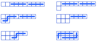
Figure 6: The combinatorial procedure for the bijection $\Psi^{(1)}:[\mathscr{P}^{(2)}]_{10}\rightarrow[\mathscr{P}^{(2)}_{3}\times(\mathscr{P}_{5}\setminus\mathscr{P}_{3})]_{10}$

Having $\Psi^{(a)}$ in the proof of Proposition 13, we let $\Psi^{(a)}_{1}$ and $\Psi^{(a)}_{2}$ be the pair of maps obtained from $\Psi^{(a)}$ by composing with a projection into the first and the second component of $\mathscr{P}^{(n)}_{n+a}\times(\mathscr{P}_{2n+a}\setminus\mathscr{P}_{n+a})$, respectively.

Corollary 14.

There is an energy preserving bijection between $\mathscr{P}^{(n)}\times\mathscr{P}_{n+a}$ and $\mathscr{P}^{(n)}_{n+a}\times\mathscr{P}_{2n+a}$.

Proof.

We define the map $\Phi^{(a)}:\mathscr{P}^{(n)}\times\mathscr{P}_{n+a}\rightarrow\mathscr{P}^{(n)}_{n+a}\times\mathscr{P}_{2n+a}$ as follows. Given an element $(\nu,\pi)\in\mathscr{P}^{(n)}\times\mathscr{P}_{n+a}$, let $\Phi^{(a)}(\nu,\pi)=(\Psi^{(a)}_{1}(\nu),\Psi^{(a)}_{2}(\nu)\cup\pi)$ . Clearly this $\Phi^{(a)}$ gives the desired bijection. ∎

7 Proof of the main result

In this section, we give a proof of Theorem 1 to establish the main result of this paper.

Let $\lambda\in\mathscr{P}$, and recall the definitions of the Durfee square/rectangle $D_{a}(\lambda)$, its vertical side $n_{a}=n_{a}(\lambda)$, the sub-diagram $A_{a}(\lambda)$, and the residual diagram $R_{a}(\lambda)$ used to evaluate its squrank/recrank. In $\lambda$, the cells inside the first $n_{a}+a$ columns but not in $D_{a}(\lambda)$ constitute a sub-diagram of $\lambda$. Let $L_{a}(\lambda)$ denote this sub-diagram. In other words, we have a unique decomposition

$$\lambda=D_{a}(\lambda)\uplus A_{a}(\lambda)\uplus L_{a}(\lambda),$$ (37)

for every partition $\lambda$, where $\uplus$ denotes disjoint union. Note that $A_{a}(\lambda)\in\mathscr{P}^{(n)}$ and $L_{a}(\lambda)\in\mathscr{P}_{n+a}$ with $n=n_{a}(\lambda)$.

Example 8.

Let $\lambda=(19,16,9,2,1)$. Then we have $L_{0}(\lambda)=L_{1}(\lambda)=(2,1)$. See Figs 2 and 3 for the relevant decomposition of the diagram into the sub-diagrams given by the right hand side of (37).

By comparing the procedure to define squrank/recrank and the procedure to define $\Psi^{(a)}$ in the proof of Proposition 13, we see that $R_{a}(\lambda)=\Psi^{(a)}_{1}(A_{a}(\lambda))\in\mathscr{P}^{(n)}_{n+a}$ with $n=n_{a}(\lambda)$. Thus in terms of the map $\Psi^{(a)}_{1}$ the definition of squrank/recrank takes the form

$${\rm squrank}(\lambda) =\mathcal{E}_{1}(\Psi^{(0)}_{1}(A_{0}(\lambda));n_{0}(\lambda)),$$ (38)

$${\rm recrank}(\lambda) =\mathcal{E}_{1}(\Psi^{(1)}_{1}(A_{1}(\lambda));n_{1}(\lambda)),$$ (39)

where $\mathcal{E}_{1}$ is the function defined in (34). Now we define

$$\mathscr{S}^{[n;r]} =\{\lambda\in\mathscr{P}\mid{\rm squrank}(\lambda)=r,n_{0}(\lambda)=n\},$$ (40)

$$\mathscr{R}^{[n;r]} =\{\lambda\in\mathscr{P}\mid{\rm recrank}(\lambda)=r,n_{1}(\lambda)=n\}.$$ (41)

Recall the definition of $\Phi^{(a)}:\mathscr{P}^{(n)}\times\mathscr{P}_{n+a}\rightarrow\mathscr{P}^{(n)}_{n+a}\times\mathscr{P}_{2n+a}$ in the proof of Corollary 14 and the decomposition (37). By using the relation

$$\Phi^{(a)}(A_{a}(\lambda),L_{a}(\lambda))=(\Psi^{(a)}_{1}(A_{a}(\lambda)),\Psi_{2}^{(a)}(A_{a}(\lambda))\cup L_{a}(\lambda)),$$ (42)

and noting that the map $\Phi^{(a)}$ is an energy preserving bijection, we see that

$$\sum_{\lambda\in\mathscr{S}^{[n;r]}}q^{|\lambda|} =q^{n^{2}}\cdot\sum_{\pi\in\mathscr{P}^{(n;r)}_{n}}q^{|\pi|}\cdot\sum_{\mu\in\mathscr{P}_{2n}}q^{|\mu|},$$ (43)

$$\sum_{\lambda\in\mathscr{R}^{[n;r]}}q^{|\lambda|} =q^{n^{2}+n}\cdot\sum_{\pi\in\mathscr{P}^{(n;r)}_{n+1}}q^{|\pi|}\cdot\sum_{\mu\in\mathscr{P}_{2n+1}}q^{|\mu|},$$ (44)

where $\mathscr{P}^{(n;r)}_{n+a}$ is the subset of $\mathscr{P}^{(n)}_{n+a}$ given by (35). Now we define

$${\rm ps}^{(r)}(n) =\#\{\lambda\vdash n\mid{\rm squrank}(\lambda)=r\},$$ (45)

$${\rm pr}^{(r)}(n) =\#\{\lambda\vdash n\mid{\rm recrank}(\lambda)=r\}.$$ (46)

Then by using (36), (43), and (44), we have

$$\sum_{n\geq 0}{\rm ps}^{(r)}(n)q^{n} =\sum_{n\geq 0}\frac{q^{n^{2}}Z_{2n,n}^{(r)}(q)}{(q;q)_{2n}},$$

$$\sum_{n\geq 0}{\rm pr}^{(r)}(n)q^{n} =\sum_{n\geq 0}\frac{q^{n^{2}+n}Z_{2n+1,n}^{(r)}(q)}{(q;q)_{2n+1}}.$$

Comparing this result with Proposition 3, we see that $p^{(r)}_{2,1}(n)={\rm ps}^{(r)}(n)$ and $p^{(r)}_{2,2}(n)={\rm pr}^{(r)}(n)$. This completes the proof of Theorem 1.

8 Concluding remarks

Inspired by the study of the minimal excludant in integer partitions by Andrews and Newman [4], and in particular by the generating function (9) of the mex-related function $p_{2,2}(n)$, we introduced a pair of partition statistics, squrank and recrank. We have shown that there is a nontrivial connection between these statistics and the odd/even mex functions for having equinumerous integer partitions. To establish our main result, Theorem 1, we used an analytic method for showing that the different partition statistics share the same generating functions. We hope that there is a more explicit bijective proof of our result.

An obvious generalization of our answer (Corollary 2) to one of their questions [4, p. 9, Question II] may be stated as follows: $p_{2,1}(n)$ equals the number of partitions of $n$ with even squrank. However, as was shown in their paper [4, Theorem 4], there is a simpler partition statistic which produces the same integer sequence $\{p_{2,1}(n)\}_{n\geq 0}$. In fact, there is the identity $p_{2,1}(n)=p_{e}(n)$ where $p_{e}(n)$ is the number of partitions of $n$ into an even numbers of parts. The author does not know whether a similar result exists for $p_{2,2}(n)$.

The author believes that most of the readers will agree to saying that the definition of our new partition statistics in Sect. 2 is fairly succinct. However, while the definition of rank and crank was stated in three lines without using mathematical notation [4], our definition of squrank and recrank requires ten lines. While the former only uses parts and number of parts of the partitions, the latter uses Ferrers diagrams and combinatorial procedures thereon. This may be rather unsatisfactory. We hope that someone will be able to find another partition statistic with more succinct definition but can reproduce the same integer sequence by $p_{2,2}(n)$.

References

- [1] Andrews, G.E.: The Theory of Partitions, Cambridge Univ. Press, New York (1984)
- [2] Andrews, G.E., Baxter, R.J., Forrester, P.J.: Eight-vertex SOS model and generalized Rogers-Ramanujan-type identities, Journal of Statistical Physics 35, 193–266 (1984)
- [3] Andrews, G.E., Garvan, F.G.: Dyson’s crank of a partition, Bulletin (New Series) of the American Mathematical Society 18, 167–171 (1988)
- [4] Andrews, G.E., Newman, D.: The minimal excludant in integer partitions, Journal of Integer Sequences 23, Article 20.2.3. (2020)
- [5] Chern, S.: -Log-concavity and -unimodality of Gaussian polynomials and a problem of Andrews and Newman, Proc. Japan Acad., 99 Ser. A, 33–36 (2023)
- [6] Croydon, D.A., Kato, T., Sasada, M., Tsujimoto, S.: Dynamics of the Box-Ball System with Random Initial Conditions via Pitman’s Transformation, Memoirs of the American Mathematical Society 283 no. 1398, (2023)
- [7] Dyson, F.J.: Some guesses in the theory of partitions, Eureka 8, 10–15 (1944)
- [8] Kang, S-J., Kashiwara, M., Misra, K.C., Miwa, T., Nakashima, T., Nakayashiki, A.: Affine crystals and vertex models, Int. J. Mod. Phys. A7 (suppl. 1A), 449–484 (1992)
- [9] Kuniba, A., Okado, M., Takagi, T.,Yamada, Y.: Vertex operators and canonical partition functions of the box-ball system (in Japanese), RIMS Kkyroku, 1302, 91–107 (2003)
- [10] Macdonald, I.G.: Symmetric Functions and Hall Polynomials, 2nd ed., Clarendon Press, Oxford (1995).
- [11] Sagan, B.E.: The Symmetric Group — Representations, Combinatorial Algorithms, and Symmetric Functions, 2nd Ed., Springer-Verlag, New York, (2000)
- [12] Schilling, A.: Multinomials and polynomial bosonic forms for the branching functions of the conformal coset models, Nuclear Physics B, 467, 247–271 (1996)
- [13] Takagi, T.: Inverse scattering method for a soliton cellular automaton, Nuclear Physics B 707, 577–601 (2005)
- [14] Takagi, T.: A bosonic formula for one-dimensional configuration sums and the even minimal excludant in integer partitions, Scientific and Engineering Reports of the National Defense Academy, Japan (in Japanese), 62 No. 1·2, to appear (2025)