Inequalities between Dirichlet and Neumann Eigenvalues on Surfaces

Abstract.

For a bounded Lipschitz domain $\Sigma$ in a Riemannian surface $M$ satisfying certain curvature condition, we prove that for any $k\geq 1,$ we have

$$\mu_{k+2-\beta_{1}}\leq\lambda_{k},$$

where $\mu_{k}$ ($\lambda_{k}$ resp.) is the $k$-th Neumann (Dirichlet resp.) Laplacian eigenvalue on $\Sigma$ and $\beta_{1}$ is the first Betti number of $\Sigma.$ This extends previous results on the Euclidean space to curved surfaces, including the flat cylinder, the hyperbolic plane, hyperbolic cusp, funnel, etc. The novelty of the paper lies in comparing Dirichlet and Neumann Laplacian eigenvalues via the variational principle of the Hodge Laplacian on $1$-forms on a surface, extending the variational principle on vector fields in the Euclidean plane as developed by Rohleder [50]. The comparison is reduced to the existence of a distance function with appropriate curvature conditions on its level sets.

Keywords: Dirichlet and Neumann eigenvalue, Friedlander’s inequality, variational principle, hyperbolic geometry.

1. Introduction

Spectral theory of Laplace operators on Euclidean spaces or Riemannian manifolds is fundamental in partial different equations, geometry and physics, which was extensively studied in the literature, see e.g. [22, 49, 48, 17, 52]. For eigenvalues of the Laplacian on a bounded domain, the boundary condition, Dirichlet or Neumann, has strong physical meaning and is of significant importance in the studies. There are many results on such eigenvalue estimates, see e.g. [56, 54, 55, 44, 47, 41, 59, 6, 5, 20, 18, 14, 58].

For a given domain, finding intrinsic relationship between Dirichlet eigenvalues and Neumann eigenvalues is an interesting topic. We recall some related results on the Euclidean spaces. For a bounded Lipschitz domain $\Sigma\subset\mathbb{R}^{n},$ denote by $\mu_{k}$ ($\lambda_{k}$ resp.) the $k$-th eigenvalue of the Laplacian on $\Sigma$ with Neumann (Dirichlet resp.) boundary condition, ordered by

$$0=\mu_{1}<\mu_{2}\leq\mu_{3}\leq\cdots,\quad(0<\lambda_{1}<\lambda_{2}\leq\lambda_{3}\leq\cdots\mathrm{resp.}).$$

By the classical variational principle, one immediately has $\mu_{k}\leq\lambda_{k}$ for all $k\in\mathbb{Z}_{+}$. In 1952, Pólya [46] proved that $\mu_{2}<\lambda_{1}$ for any bounded Lipschitz domain in $\mathbb{R}^{2}.$ Later, Payne [43] proved that $\mu_{k+2}<\lambda_{k}$ for all $k\in\mathbb{Z}_{+}$ for a bounded convex domain with $C^{2}$ boundary in $\mathbb{R}^{2}.$ In 1991, Friedlander [28] established that $\mu_{k+1}\leq\lambda_{k}$ for all $k\in\mathbb{Z}_{+}$ for any bounded $C^{1}$ domain in $\mathbb{R}^{n},$ which is now called Friedlander’s inequality. For more results in this direction, one refers to [8, 54, 42, 40, 34, 37, 27, 2, 23, 26, 29, 51, 7, 31].

Recently, Rohleder [50] introduce an innovative method based on the variational principle for vector fields on the plane, combined with Helmholtz decomposition, to prove that $\mu_{k+2}\leq\lambda_{k},k\in\mathbb{Z}_{+}$ for any simply-connected and bounded Lipschitz domain in $\mathbb{R}^{2}$. This removes the convexity condition for domains in Payne’s result [43], and extends Friedlander’s inequality.

In this paper, we aim to extend Rohleder’s method to general Riemannian surfaces and prove the comparison result for Dirichlet and Neumann eigenvalues. We require the following two ingredients: On one hand, Rohleder introduced a linear operator on vector fields defined on the planar domain, whose spectrum consists of Dirichlet and Neumann Laplacian eigenvalues. However, its geometric meaning is not clear for a general surface. Our key observation is that the spectrum of the Hodge Laplacian on $1$-forms, with the appropriate boundary conditions, serves the same purpose on surfaces. Using this, we can apply the standard variational principle and the Hodge decomposition to compare the Dirichlet and Neumann eigenvalues. On the other hand, we need suitable test functions for the variational arguments, which are provided by the following curvature condition. A $C^{1}$ function $f$ on a Riemannian surface $M$ is called a distance function if it has unit gradient, i.e. $|\nabla f|\equiv 1.$

Definition 1.1.

We say a domain $\Sigma$ in a Riemannian surface $M$ satisfies the curvature condition if there exist an open set $U\supset\overline{\Sigma}$ and a distance function with $f\in C^{3}(U)$ such that the Gaussian curvature $K$ satisfies

$$K\leq-|\operatorname{Hess}f|^{2}\quad\text{in }U.$$ (1)

For convenience, we also say that $f$ satisfies the curvature condition in $U$.

One easily sees that the necessary condition for the above is the non-possitivity of the Gaussian curvature. Moreover, the planar domain satisfies the curvature condition by choosing the coordinate function as the distance function. For a smooth distance function $f,$ the sufficient and necessary condition for (1) is

$$K(x)\leq-h^{2}(x)\quad\forall x\in U,$$ (2)

where $h(x)$ is the curvature of the level set $f^{-1}(f(x)).$ This justifies the term “curvature condition”, and relax the requirement in [42] demanding for a constant mean curvature of level sets. Later, we will provide several interesting examples that satisfy the curvature condition, including warped product surfaces with log-convex warped functions, the flat cylinder, the hyperbolic plane, hyperbolic cusp, funnel, etc. The following is the main result of the paper.

Theorem 1.2.

Let $\Sigma$ be a bounded Lipschitz domain in a Riemannian surface $M$ satisfying the curvature condition. Then

$$\mu_{k+2-\beta_{1}}\leq\lambda_{k},\quad\,\forall\,k\in\mathbb{Z}_{+},$$ (3)

where $\beta_{1}$ is the first Betti number of $\Sigma.$

Remark 1.3.

The result is meaningful only when $\beta_{1}=0$ or $1,$ since it is trivial for $\beta_{1}\geq 2.$ For the case of $\mathbb{R}^{2},$ it recovers Rohleder’s result [50] for a simply-connected bounded Lipschitz domain. This theorem generalizes the result to the surface case satisfying the curvature condition.

The proof strategy of the theorem is as follows: First, for a smooth bounded domain, we introduce the Hodge Laplacian on $1$-forms with appropriate boundary conditions, whose spectrum consists of Dirichlet and Neumann Laplacian eigenvalues (see Proposition 4.2). On a surface, the Hodge Laplacian on $1$-forms decomposes into the upward and downward Laplacians. The spectrum of the upward (downward resp.) Laplacian coincides with that of the Hodge Laplacian on $2$-forms ($0$-forms resp.), up to some null eigenvalues, and corresponds to the Dirichlet (Neumann resp.) Laplacian eigenvalues. This is a crucial property in dimension two, which is difficult to generalize to higher dimensions. Second, we utilize Dirichlet eigenfunctions to construct specific $1$-forms, adopt suitable test functions provided by the curvature condition, and apply the variational principle for the Hodge Laplacian of $1$-forms to compare the Dirichlet and Neumann eigenvalues. Finally, we approximate the Lipschitz domain from the exterior by a sequence of smooth domains with a uniform cone condition. We prove the lower semi-continuity of the Neumann eigenvalues for the approximating sequence and extend the result to Lipschitz domains (see Appendix).

Theorem 1.2 reduces this problem to finding an appropriate distance function on the surface that satisfies the curvature condition in Definition 1.1. For applications, we discuss the curvature condition as follows. The first candidate is the Busemann function on a Hadamard surface, which is a simply-connected surface with nonpositive curvature. This function is a natural distance function to infinity. For a space form of nonpositive curvature, such as the plane or the hyperbolic plane, the Busemann function satisfies the curvature condition; see Example 5.6 (or [16]) for the hyperbolic case. In a general Hadamard surface, it remains an interesting question whether there exists a Busemann function that satisfies the curvature condition. See, e.g., [32, 36, 35] for discussions of Busemann functions.

The next theorem provides a criterion for the curvature condition in a twisted product surface.

Theorem 1.4.

Let $M=(I\times S^{1},g),$ for an interval $I\subset\mathbb{R},$ be a twisted product surface with the metric

$$g(r,\theta)=dr^{2}+\phi(r,\theta)^{2}d\theta^{2},\quad(r,\theta)\in M,$$

where $\phi$ is a positive smooth function. Then the radius distance function $f(r,\theta)=r$ satisfies the curvature condition if and only if $\phi(r,\theta)$ is log-convex in $r$, that is, $\partial^{2}_{r}\log\phi\geq 0$. In this case, every bounded Lipschitz domain $\Sigma\subset M$ satisfies the eigenvalue inequality (3).

Remark 1.5.

When $\phi=\phi(r)$ does not depend on $\theta$, the twisted product structure simplifies to the well-known warped product. There are plenty of examples of warped product surfaces with log-convex warped functions. For example, one chooses $\phi=e^{f}$ for any convex function $f$ on $I.$ Typical examples are as follows:

1. Flat cylinder on $\mathbb{R}\times S^{1}$ with $\phi=\mathrm{const.};$

2. Hyperbolic cusp on $\mathbb{R}\times S^{1}$ with $\phi(r)=e^{r},$ see Example 5.8.

3. Hyperbolic collar (funnel resp.) on $\mathbb{R}\times S^{1}$ ($[0,+\infty)\times S^{1}$ resp.) with $\phi(r)=\cosh r,$ see Example 5.9 for collars. In fact, $\phi$ satisfies the log-convex condition strictly, thus we allow a compact supported perturbation of the metric, i.e.

   $$\phi=\cosh r+\varepsilon g(r,\theta),\quad g\geq 0,\quad g\in C_{c}^{\infty},\quad\varepsilon>0\text{ is sufficiently small.}$$

The fundamental structures in hyperbolic geometry consist of cusps, funnels, and collars. In a complete hyperbolic surface, the ends are either cusps or funnels, and there exists a neighborhood of simple closed geodesics forming a collar [10, 15]. All of them satisfy the curvature conditions, and hence our results apply to hyperbolic geometry. We collect them in the following corollary.

Corollary 1.6.

Let $M$ be a space form with a nonpositive curvature, flat cylinder, hyperbolic cusp, funnel, or collar. For any bounded Lipschitz domain $\Sigma\subset M,$ the inequality (3) holds.

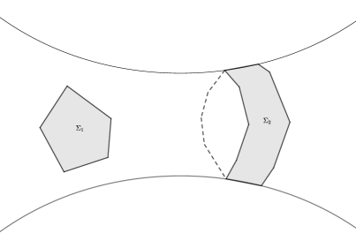
Figure 1. Bounded Lipschitz domains in a cusp and a collar. As $\Sigma_{1}$ is simply connected, we have $\mu_{k+2}\leq\lambda_{k}$. While for annular domain $\Sigma_{2},$ we can only obtain $\mu_{k+1}\leq\lambda_{k}.$

Remark 1.7.

Note that Mazzeo [42] proved Friedlander’s inequality on hyperbolic plane, and our result improves his estimate from $\mu_{k+1}$ to $\mu_{k+2}$ for simply-connected bounded domains. The cases of cylinders, cusps, funnels and collars are noteworthy and have not been investigated previously. Moreover, eigenvalue estimates for cusps, funnels and collars are novel contributions, since they are fundamental structures in hyperbolic surfaces.

The paper is organized as follows: we introduce basic concepts of differential forms and Hadamard manifolds in Section 2. Section 3 contains the theory of Sobolev spaces for differential forms based on [53]. Section 4 is devoted to necessary analytical tools: spectral decomposition for the Hodge Laplacian, Dirichlet form, and variational principle. In Section 5, we prove the main theorems and provide several examples in detail. The smooth approximation of a Lipschitz domain and the semi-continuity of Neumann eigenvalues is included in the Appendix.

2. Preliminaries

2.1. Notations for Differential Forms

Let $(M^{n},g)$ be an oriented $n$-dimensional Riemannian manifold. We consider the exterior $k$-form bundle $\Lambda^{k}(M)$ and its smooth sections $\Omega^{k}(M)=\Gamma(\Lambda^{k}(M))$, which constitute the space of differential forms of degree $k$ on $M$, where $k\in\mathbb{N}$.

Using the musical isomorphism $\sharp:T^{*}_{p}M\rightarrow T_{p}M$ defined by

$$g(\omega^{\sharp},v)=\omega(v),\quad\forall v\in T_{p}M,$$

we can define the pointwise inner product on $\Lambda^{1}(M)$ as

$$\langle\omega,\nu\rangle=g(\omega^{\sharp},\nu^{\sharp}),$$

which extends to $\Lambda^{k}(M)$ by

$$\langle\omega_{1}\wedge\cdots\wedge\omega_{k},\nu_{1}\wedge\cdots\wedge\nu_{k}\rangle=\det\{\langle\omega_{i},\nu_{j}\rangle\}_{i,j=1}^{k}.$$

The inverse map of $\sharp$ is denoted by $\flat:T_{p}M\rightarrow T^{*}_{p}M$, and both maps naturally extend to isomorphisms between $TM$ and $T^{*}M$.

We denote the volume form by $\operatorname{vol}_{M}\in\Omega^{n}(M)$, which satisfies

$$\operatorname{vol}_{M}(X_{1},\ldots,X_{n})=\sqrt{\det\{g(X_{i},X_{j})\}_{i,j=1}^{n}}.$$

The Hodge operator $*:\Omega^{k}(M)\rightarrow\Omega^{n-k}(M)$ is defined by

$$\omega\wedge(*\nu)=\langle\omega,\nu\rangle\operatorname{vol}_{M},\quad\forall\omega\in\Omega^{k}(M).$$

Proposition 2.1 ([39]).

The Hodge operator satisfies the following properties for all $\omega,\nu\in\Omega^{k}(M)$:

1. $*(*\omega)=(-1)^{k(n-k)}\omega,$

2. $\langle*\omega,*\nu\rangle=\langle\omega,\nu\rangle.$

Suppose $\Sigma\subset M$ is a compact $n$-dimensional submanifold with boundary, equipped with an induced atlas, also known as the $\partial$-manifold in [53]. Differential forms on $\Sigma$ are denoted by $\Omega^{*}(\Sigma)$. Let $\iota:\Sigma\rightarrow M$ be the inclusion map, then we have $\iota^{*}\Omega^{*}(M)\subset\Omega^{*}(\Sigma)$.

The $L^{2}$ inner product on $\Omega^{k}(\Sigma)$ is defined by

$$(\omega_{1},\omega_{2}):=\int_{\Sigma}\langle\omega_{1},\omega_{2}\rangle\operatorname{vol}_{M}=\int_{\Sigma}\omega_{1}\wedge(*\omega_{2}),\quad\omega_{1},\omega_{2}\in\Omega^{k}(\Sigma).$$

The co-differential operator is defined by $d^{*}\omega:=(-1)^{nk+n+1}*d(*\omega)$ for $\omega\in\Omega^{k}(\Sigma)$. By Stokes’ theorem, we have the following lemma.

Lemma 2.2 (Green’s Formula).

Let $i:\partial\Sigma\rightarrow\Sigma$ be the inclusion map. Then, for $\omega_{1}\in\Omega^{k-1}(\Sigma)$ and $\omega_{2}\in\Omega^{k}(\Sigma)$, we have

$$(d\omega_{1},\omega_{2})=(\omega_{1},d^{*}\omega_{2})+\int_{\partial\Sigma}i^{*}(\omega_{1}\wedge*\omega_{2}).$$ (4)

Proof.

Let $\omega=\omega_{1}\wedge*\omega_{2}$. Then,

$$d\omega =d\omega_{1}\wedge*\omega_{2}+(-1)^{k-1}\omega_{1}\wedge(d*\omega_{2})$$

$$=d\omega_{1}\wedge*\omega_{2}+(-1)^{nk+n+k}*\omega_{1}\wedge d^{*}\omega_{2}$$

$$=d\omega_{1}\wedge*\omega_{2}+(-1)^{nk+n+k+(k-1)(n-k+1)}d^{*}\omega_{2}\wedge*\omega_{1}$$

$$=d\omega_{1}\wedge*\omega_{2}-d^{*}\omega_{2}\wedge*\omega_{1}.$$

Thus, by Stokes’ theorem, we obtain

$$\int_{\partial\Sigma}i^{*}\omega=\int_{\Sigma}d\omega=\int_{\Sigma}d\omega_{1}\wedge*\omega_{2}-\int_{\Sigma}d^{*}\omega_{2}\wedge*\omega_{1}=(d\omega_{1},\omega_{2})-(d^{*}\omega_{2},\omega_{1}).$$

Reorganizing terms completes the proof. ∎

Example 2.3.

For $M=\mathbb{R}^{2}$, it is straightforward to see that for a vector field $v=u_{1}e_{1}+u_{2}e_{2}\in\Gamma(T\Sigma)$, we have $v^{\flat}=u_{1}dx_{1}+u_{2}dx_{2}\in\Omega^{1}(\Sigma)$. Then,

$$d(v^{\flat})=(\partial_{1}u_{2}-\partial_{2}u_{1})\operatorname{vol}_{M}=(\operatorname{curl}v)\operatorname{vol}_{M}.$$

For the Hodge operator, we have

$$*dx_{1}=dx_{2},\quad*dx_{2}=-dx_{1},\quad*(v^{\flat})=u_{1}dx_{2}-u_{2}dx_{1}=(v^{\perp})^{\flat},$$

where $v^{\perp}:=-u_{2}e_{1}+u_{1}e_{2}$ is the vector $v$ rotated by $\frac{\pi}{2}$ counterclockwise. Then we obtain

$$-d^{*}(v^{\flat})=*d(u_{1}dx_{2}-u_{2}dx_{1})=\partial_{1}u_{1}+\partial_{2}u_{2}=\operatorname{div}v.$$

The Hodge Laplacian is defined as $\Delta_{k}:=d^{*}d+dd^{*}$ on $k$-forms. Naturally, we have $d^{*}|_{\Omega^{0}(\Sigma)}=0$ and $d|_{\Omega^{n}(\Sigma)}=0$. We may omit the subscript $k$ when the degree is clear from the context.

2.2. Busemann Function on a Hadamard Manifold

Suppose $H$ is a Hadamard manifold, meaning $H$ is a simply-connected and complete Riemannian manifold with non-positive sectional curvature everywhere. By the Cartan-Hadamard theorem, $H$ is diffeomorphic to $\mathbb{R}^{n}$.

Let $\gamma_{1}$ and $\gamma_{2}$ be two geodesic rays, $\gamma_{i}:[0,\infty)\rightarrow H$, $i=1,2$. We always consider geodesics with unit speed. The geodesics $\gamma_{1}$ and $\gamma_{2}$ are said to be asymptotically equivalent if there exists a constant $C>0$ such that $d(\gamma_{1}(t),\gamma_{2}(t))<C$ for all $t\geq 0$. The set of all asymptotically equivalent classes forms the ideal boundary of $H$, denoted by $\partial H$. This boundary can be regarded as the “point at infinity” of $H$, meaning that a geodesic $\gamma$ is said to “converge” to $\theta\in\partial H$ at infinity if $\gamma$ represents the class $\theta$.

Fix an arbitrary point $o\in H$ and let $\theta\in\partial H$. We can find a unique geodesic ray such that $\gamma(0)=o$ and $[\gamma]=\theta$. The corresponding Busemann function is defined as

$$B_{\theta}(x):=\lim_{t\rightarrow\infty}\left(d(x,\gamma(t))-t\right).$$

Proposition 2.4 ([36]).

The Busemann function $B_{\theta}$ satisfies the following properties:

1. $B_{\theta}$ is a convex function with $C^{2}$ regularity.

2. $|dB_{\theta}|\equiv 1$.

The level set of $B_{\theta}$ containing $x\in H$ is called a horosphere centered at $\theta$ passing through $x$, denoted by $\mathcal{H}_{(x,\theta)}$, i.e.,

$$\mathcal{H}_{(x,\theta)}=\{y\in H\mid B_{\theta}(y)=B_{\theta}(x)\}.$$

By the implicit function theorem, the horosphere $\mathcal{H}_{(x,\theta)}$ has $C^{2}$ regularity.

The gradient field $\nabla B_{\theta}$, when restricted to $\mathcal{H}_{(x,\theta)}$, yields the $C^{1}$ unit vector field $N$ that is outward normal to $\mathcal{H}_{(x,\theta)}$. The second fundamental form is given by the Hessian

$$h(v,w)=\langle-\nabla_{v}N,w\rangle=-\nabla^{2}B_{\theta}(v,w),\quad v,w\in T_{y}\mathcal{H}_{(x,\theta)}.$$

This form is negative semi-definite because $B_{\theta}$ is convex.

3. Sobolev Space for Differential Forms

3.1. General Case

The form space $L^{2}\Omega^{k}(\Sigma)$ is defined as the completion of $\Omega^{k}(\Sigma)$ with respect to the induced norm

$$\|\omega\|_{L^{2}}:=\sqrt{(\omega,\omega)}.$$

Moreover, the Sobolev space $H^{s}\Omega^{k}(\Sigma)$ is defined as the completion of $\Omega^{k}(\Sigma)$ with respect to the norm

$$\|\omega\|_{H^{s}}:=\sqrt{\sum_{r=0}^{s}\|\nabla^{r}\omega\|_{L^{2}}^{2}},\quad s\geq 0,$$ (5)

where $\nabla$ is the Levi-Civita connection on $M$. Similarly, one can define $W^{s,p}\Omega^{k}(\Sigma)$ more generally; see [53]. For $s<0$, the corresponding Sobolev space is defined as the dual space of $H^{-s}.$

It is clear that these spaces are Hilbert spaces with the corresponding inner product. Since $\|\omega\|_{L^{2}}=\|*\omega\|_{L^{2}}$ for all $\omega\in\Omega^{k}(\Sigma)$, the Hodge star operator has a continuous extension

$$*:L^{2}\Omega^{k}(\Sigma)\rightarrow L^{2}\Omega^{n-k}(\Sigma),$$

and it is an isometry. Given that $*(\nabla_{Y}\omega)=\nabla_{Y}(*\omega)$ for all $Y\in T\Sigma$ and $\omega\in\Omega^{k}(\Sigma)$, we also have $\|\omega\|_{H^{s}}=\|*\omega\|_{H^{s}}$, and thus the Hodge star operator extends to an isometry between Sobolev spaces as well.

By the standard theory of Sobolev spaces [53], regarding the trace, we have

$$\|i^{*}\omega\|_{H^{s}\Omega^{k}(\partial\Sigma)}\leq\|\omega|_{\partial\Sigma}\|_{H^{s}\Gamma(\Lambda^{k}(\partial\Sigma))}\leq C\|\omega\|_{H^{s+1}\Omega^{k}(\Sigma)},$$

from which we obtain the continuous (and compact) linear map

$$i^{*}:H^{s+1}\Omega^{k}(\Sigma)\rightarrow H^{s}\Omega^{k}(\partial\Sigma),\quad s\geq 0.$$

The differential operators $d$ and $d^{*}$ continuously extend to the Sobolev space such that

$$d:H^{s+1}\Omega^{k}(\Sigma)\rightarrow H^{s}\Omega^{k+1}(\Sigma),\quad d^{*}:H^{s+1}\Omega^{k}(\Sigma)\rightarrow H^{s}\Omega^{k-1}(\Sigma),\quad s\geq 0,$$

as both can be expressed using $\nabla$ after choosing a coordinate system.

By the continuity of the exterior derivative and the trace formula, Stokes’ theorem can be shown to hold for Sobolev spaces as well, allowing us to extend Green’s formula (4) to Sobolev spaces. Specifically, we have

$$(d\omega_{1},\omega_{2})=(\omega_{1},d^{*}\omega_{2})+\int_{\partial\Sigma}i^{*}(\omega_{1}\wedge*\omega_{2}),\quad\forall\omega_{1}\in H^{1}\Omega^{k-1}(\Sigma),\>\omega_{2}\in H^{1}\Omega^{k}(\Sigma).$$ (6)

We define the following form space for $s\geq 1$:

$$H^{s}\Omega_{D}^{k}(M)=\{\omega\in H^{s}\Omega^{k}(M)\mid i^{*}(*\omega)=0\}.$$ (7)

As we will see later, this condition represents the absence of a normal component for forms at the boundary. The subscript $D$ represents exactly the Dirichlet condition.

Using standard techniques for elliptic equations, we can derive the following Hodge decomposition on the $\partial$-manifold $\Sigma$, which will be crucial in our paper.

Theorem 3.1 ([53], Corollary 2.4.9).

Let $\Sigma$ be a $\partial$-manifold. We have the following $L^{2}$-orthogonal decomposition:

$$L^{2}\Omega^{k}(\Sigma)=dH^{1}\Omega^{k-1}(\Sigma)\oplus d^{*}H^{1}\Omega^{k+1}_{D}(\Sigma)\oplus\mathcal{H}^{k}_{D}(\Sigma),$$ (8)

where $\mathcal{H}^{k}_{D}(\Sigma)$ is the harmonic form with Dirichlet boundary defined as

$$\mathcal{H}^{k}_{D}(\Sigma):=\{\omega\in H^{1}\Omega^{k}_{D}(\Sigma)\mid d\omega=0,\,d^{*}\omega=0\}.$$

Moreover, we have the following Hodge isomorphism.

Theorem 3.2 ([53], Theorem 2.6.1).

For the $k$-th cohomology group $H^{k}_{dR}(\Sigma)$, we have

$$H^{k}_{dR}(\Sigma)\cong\mathcal{H}^{k}_{D}(\Sigma).$$

When $\Sigma$ is simply-connected, we have $\mathcal{H}^{k}_{D}(\Sigma)=0,$ and (8) only has the leading two spaces. This case is also known as Helmholtz decomposition when we are dealing with vector fields on plane.

3.2. Surface Case

In this subsection, we will primarily focus on the case when $n=2$ to avoid extensive discussion on fractional Sobolev spaces for differential forms. Generally, fractional Sobolev spaces for differential forms can be defined on Euclidean space, and then the corresponding spaces on a manifold can be defined using a partition of unity, with some uniform curvature assumption if the area is not compact.

Consider the space

$$\mathscr{E}(\Sigma):=\{\omega\in L^{2}\Omega^{1}(\Sigma)\mid d^{*}\omega\in L^{2}\Omega^{0}(\Sigma)=L^{2}(\Sigma)\}$$

with the corresponding norm

$$\|\omega\|^{2}_{\mathscr{E}}:=\|\omega\|^{2}_{L^{2}}+\|d^{*}\omega\|^{2}_{L^{2}}.$$

This is a Hilbert space, and $\Omega^{1}(\Sigma)$ is dense in $\mathscr{E}(\Sigma)$ under this norm.

Let $\nu$ be the outer normal vector of $\partial\Sigma$. The mapping

$$\Omega^{1}(\Sigma)\ni\omega\mapsto\omega|_{\partial\Sigma}(\nu)$$

extends to the map $\mathscr{E}(\Sigma)\rightarrow H^{-\frac{1}{2}}(\partial\Sigma)$; see [24, Chapter XIX, §1, Theorem 2] for the case on plane $\mathbb{R}^{2}$. The situation is similar for manifolds, particularly for Hadamard surface as there is a direct isomorphism to the plane, and when we focus on a compact area.

In fact, we have

$$i^{*}(*\omega)=\omega|_{\partial\Sigma}(\nu)\operatorname{vol}_{\partial\Sigma},$$

so $i^{*}(*\omega)$ can be used to express the boundary condition as in (7). Notably, Green’s formula (4) extends to $\mathscr{E}(\Sigma)$ as follows:

$$(du,\omega)=(u,d^{*}\omega)+\int_{\partial\Sigma}i^{*}(*\omega)u,\quad\forall u\in H^{1}(\Sigma),\,\omega\in\mathscr{E}(\Sigma).$$ (9)

Similarly, for all $\omega\in*\mathscr{E}(\Sigma)$, we have

$$d\omega=-*(d^{*}(*\omega))\in*L^{2}(\Sigma)=L^{2}\Omega^{2}(\Sigma),$$

and therefore

$$(d\omega,A)=(\omega,d^{*}A)+\int_{\partial\Sigma}(*A)(i^{*}\omega),\quad\forall A\in H^{1}\Omega^{2}(\Sigma)=*H^{1}(\Sigma),\omega\in*\mathscr{E}(\Sigma).$$ (10)

Let $u\in H^{1}(\Sigma)$ such that $\Delta u=d^{*}du\in L^{2}(\Sigma)$ in the weak sense. Then $\omega=du\in\mathscr{E}(\Sigma)$, and hence

$$\partial_{\nu}u=du(\nu)=(*_{\partial\Sigma})i^{*}(*du)\in H^{-\frac{1}{2}}(\partial\Sigma)$$

is well-defined. We will use this to define the Neumann boundary condition.

Theorem 3.1 for the surface case with $H^{1}_{dR}(\Sigma)=0$ is the well-known Helmholtz decomposition:

$$L^{2}\Omega^{1}(\Sigma)=dH^{1}(\Sigma)\oplus d^{*}H^{1}\Omega^{2}_{D}(\Sigma)=dH^{1}(\Sigma)\oplus*dH^{1}_{0}(\Sigma).$$

4. Eigenvalue Problem on Riemannian Surfaces

4.1. Dirichlet and Neumann Problems

Consider the case when $n=2$, i.e., $M$ is a Riemannian surface, and $\Sigma$ is a bounded smooth domain on $M$. The domain of the Dirichlet problem is defined as

$$\operatorname{dom}(\Delta_{D})=\{A\in H^{1}\Omega^{2}_{D}(\Sigma)\mid\Delta A=dd^{*}A\in L^{2}\Omega^{2}(\Sigma)\},$$

and the domain of the Neumann problem is

$$\operatorname{dom}(\Delta_{N})=\{u\in H^{1}(\Sigma)\mid\Delta u=d^{*}du\in L^{2}(\Sigma),\ \partial_{\nu}u|_{\partial\Sigma}=0\}.$$

Here we note that $*\operatorname{dom}(\Delta_{D})\subset H_{0}^{1}(\Sigma)$ corresponds to the domain of the classical Dirichlet problem, and $\partial_{\nu}u|_{\partial\Sigma}$ is well-defined because $du\in\mathscr{E}(\Sigma).$ It is equivalent to say that $i^{*}(*du)=0$ for the Neumann boundary condition.

Consider the Dirichlet eigen-form $\Phi\in\operatorname{dom}(\Delta_{D})$ such that $\Delta_{D}\Phi=dd^{*}\Phi=\lambda\Phi$. Let $\Phi=\varphi\>\operatorname{vol}_{M}$, where $\varphi\in H^{1}_{0}(\Sigma)$ satisfies

$$\Delta\varphi=d^{*}d\varphi=-*d*d(**\varphi)=*dd^{*}\Phi=\lambda\varphi,$$

which is the classical eigenfunction for the Dirichlet problem on $\Sigma$.

Note that for $\varphi\in*\operatorname{dom}(\Delta_{D})\subset H_{0}^{1}(\Sigma)$, we have $d\varphi\in\mathscr{E}(\Sigma)$, and then

$$i^{*}(d\varphi)=d(i^{*}\varphi)=0.$$ (11)

Here, we use the continuity of $i^{*}$ and $d$, as well as their commutativity for smooth differential forms. For a more detailed proof, see [50, Lemma 2.2].

The Neumann eigenfunction is the classical one: $\psi\in\operatorname{dom}(\Delta_{N})$ such that $\Delta_{N}\psi=d^{*}d\psi=\mu\psi$. Denote the Neumann eigenvalues by

$$0=\mu_{1}<\mu_{2}\leq\mu_{3}\leq\cdots$$

with multiplicities, and let

$$0<\lambda_{1}<\lambda_{2}\leq\lambda_{3}\leq\cdots$$

be the eigenvalues of $\Delta_{D}$, also with multiplicities.

Take orthonormal eigenbases $(\psi_{1},\psi_{2},\cdots)$ and $(\varphi_{1},\varphi_{2},\cdots)$ of $L^{2}(\Sigma)$ such that $\Delta_{N}\psi_{i}=\mu_{i}\psi_{i}$ and $\Delta_{D}\varphi_{i}=\lambda_{i}\varphi_{i}$ hold for all $i\in\mathbb{Z}_{+}.$ Then $\{\Phi_{i}:=\varphi_{i}\operatorname{vol}_{M}\}$ form orthonormal eigenbases of $L^{2}\Omega^{2}(\Sigma)$ with $\Delta_{D}\Phi_{i}=\lambda_{i}\Phi_{i}$.

4.2. Spectral Decomposition and Dirichlet Form

Definition 4.1.

We define the Dirichlet form $\alpha$ on $H^{1}\Omega^{k}_{D}(\Sigma)$ by

$$\alpha[\omega_{1},\omega_{2}]:=(d\omega_{1},d\omega_{2})+(d^{*}\omega_{1},d^{*}\omega_{2}),$$

and we write $\alpha[\omega]:=\alpha[\omega,\omega]$ for simplicity.

Clearly, $\alpha$ is bounded since $d$ and $d^{*}$ are continuous in $H^{1}\Omega^{k}_{D}(\Sigma)$. It is semi-positive definite with the kernel being $\mathcal{H}^{k}(\Sigma)\cong H^{k}_{dR}(\Sigma)$ by Theorem 3.2.

We define the following inner product on $H^{1}\Omega^{k}_{D}(\Sigma)$:

$$(\omega_{1},\omega_{2})_{\alpha}:=\alpha[\omega_{1},\omega_{2}]+(\omega_{1},\omega_{2}).$$

By Gaffney’s inequality [53, Corollary 2.1.6], the norm induced by $(-,-)_{\alpha}$ is equivalent to the canonical $H^{1}$ norm (5) on the space $H^{1}_{D}\Omega^{k}(M)$, and we denote it by $\|-\|_{\alpha}$.

Let $A:H^{1}\Omega^{k}_{D}(\Sigma)\to H^{-1}\Omega^{k}(\Sigma)$ be the bounded $L^{2}$-self-adjoint operator such that

$$\alpha[u,v]=(Au,v),\quad\forall u,v\in H^{1}\Omega^{k}_{D}(\Sigma).$$

In fact, by Green’s formula (6), we have $Au=\Delta u$ for $u\in H^{2}\Omega^{k}_{D}(\Sigma)$ with $i^{*}(*du)=0$.

From now on, we will focus on the case where $n=2$ and $k=0,1,2$.

Proposition 4.2.

Let $\Sigma$ be a bounded smooth domain on surface. The $1$-forms $\left\{\frac{1}{\sqrt{\mu_{i}}}d\psi_{i}\right\}_{i=2}^{\infty}$ and $\left\{\frac{1}{\sqrt{\lambda_{i}}}d^{*}\Phi_{i}\right\}_{i=1}^{\infty}$ form orthonormal eigen-bases of $dH^{1}(\Sigma)$ and $d^{*}H^{1}\Omega_{D}^{2}(\Sigma)$, respectively. These eigen-bases satisfy

$$A(d\psi_{i})=\mu_{i}d\psi_{i},\quad A(d^{*}\Phi_{i})=\lambda_{i}d^{*}\Phi_{i}.$$

Let $\operatorname{Spec}_{+}$ be the positive spectrum, we have

$$\operatorname{Spec}_{+}A=\operatorname{Spec}_{+}\Delta_{D}\cup\operatorname{Spec}_{+}\Delta_{N}.$$ (12)

Proof.

For $i\geq 2$, $d\psi_{i}\in H^{1}\Omega_{D}^{1}(\Sigma)$ because $d(d\psi_{i})=0$, $d^{*}(d\psi_{i})=\mu_{i}\psi_{i}\in L^{2}(\Sigma)$, and $i^{*}(*d\psi_{i})=0$ due to the Neumann boundary condition. Similarly, $d^{*}\Phi_{i}\in H^{1}\Omega_{D}^{1}(\Sigma)$ for $i\geq 1$, and the boundary condition is satisfied by the Dirichlet condition as in (11),

$$i^{*}(*d^{*}\Phi_{i})=-i^{*}(**d*\Phi_{i})=-i^{*}(d\varphi_{i})=0.$$

Orthogonality follows from Green’s formula:

$$(d^{*}\Phi_{i},d^{*}\Phi_{j})=(dd^{*}\Phi_{i},\Phi_{j})=\lambda_{i}(\Phi_{i},\Phi_{j}),\quad(d\psi_{i},d\psi_{j})=(d^{*}d\psi_{i},\psi_{j})=\mu_{i}(\psi_{i},\psi_{j}).$$

Suppose there exists $\psi\in H^{1}(\Sigma)$ such that $d\psi\perp d\psi_{i}$ for all $i\geq 2$. Then

$$0=(d\psi,d\psi_{i})=\mu_{i}(\psi,\psi_{i}),\quad\forall i\geq 2,$$

which implies that $\psi=c\psi_{1}$ is a constant due to the orthonormality of $\{\psi_{i}\}_{i=1}^{\infty}$ in $L^{2}(\Sigma)$. Thus, $d\psi=0$, showing that $\{d\psi_{i}\}_{i=2}^{\infty}$ is orthonormal in $dH^{1}(\Sigma)$. The orthonormality of $\{d^{*}\Phi_{i}\}_{i=1}^{\infty}$ in $d^{*}H^{1}\Omega_{D}^{2}(\Sigma)$ is similar and even simpler to verify.

Finally, they are eigenforms of $A$ because for any $v\in H^{1}\Omega_{D}^{1}(\Sigma)$,

$$(Ad^{*}\Phi_{i},v)=\alpha[d^{*}\Phi_{i},v]=(dd^{*}\Phi_{i},dv)=\lambda_{i}(\Phi_{i},dv)=\lambda_{i}(d^{*}\Phi_{i},v),$$

$$(Ad\psi_{i},v)=\alpha[d\psi_{i},v]=(d^{*}d\psi_{i},d^{*}v)=\mu_{i}(\psi_{i},d^{*}v)=\mu_{i}(d\psi_{i},v).$$

Combined with the Hodge decomposition in Theorem 3.1, this proves the positive spectral decomposition (12). ∎

Remark 4.3.

In fact, one can generalize the results by replacing $\Delta_{D}$ with the downward Laplacian $L_{k}=d_{k-1}d^{*}_{k}$ and $\Delta_{N}$ with the upward Laplacian $U_{k}=d^{*}_{k+1}d_{k}$. This leads to the positive spectrum decomposition for the Laplacian $\Delta_{k}$ acting on general Sobolev $k$-forms:

$$\operatorname{Spec}_{+}\left(\Delta_{k}\right)=\operatorname{Spec}_{+}\left(U_{k-1}\right)\cup\operatorname{Spec}_{+}\left(L_{k+1}\right).$$

The proof follows a similar method to the one presented in this section. Care must be taken to properly define the corresponding spaces where these operators act.

Finally, consider the Rayleigh quotient defined by $\eta(\omega)=\frac{\alpha[\omega]}{\|\omega\|_{L^{2}}^{2}}$. Using standard variational methods, we obtain the following result:

Theorem 4.4.

Let $\eta_{1}\leq\eta_{2}\leq\cdots$ be the eigenvalues of the operator $A$. Then,

$$\eta_{k}=\min_{\begin{subarray}{c}E\subset H^{1}\Omega_{D}^{1}(\Sigma)\\ \dim E=k\end{subarray}}\max_{\omega\in E\setminus\{0\}}\eta(\omega),\quad\forall k\in\mathbb{Z}_{+}.$$

5. Friedlander’s Inequality

5.1. Proof of main theorem

In this section, we prove Theorem 1.2. It should be noted that $\Sigma$ must satisfy the curvature condition in Definition 1.1. Let $f$ be a function satisfying the curvature condition. We define $\nu:=df\in H^{1}\Omega^{1}(\Sigma)$. Consequently, $d\nu=0$, $d^{*}\nu=\Delta f$, and $|\nu|=|\nabla f|\equiv 1$.

Let $(\Phi_{i}=\varphi_{i}\mathrm{vol}_{M},\lambda_{i})$ be the Dirichlet eigenpair of $\Delta_{D}$. We obtain

$$\|\varphi_{i}\nu\|_{L^{2}}^{2}=\int_{\Sigma}\varphi_{i}^{2}|\nu|^{2}\,d\mathrm{vol}_{M}=\|\varphi_{i}\|_{L^{2}}^{2}=1.$$

Lemma 5.1.

Consider a bounded smooth domain $\Sigma$ on surface $M$ that satisfies the curvature condition. For Dirichlet eigenfunctions $\{\varphi_{i}\}_{i=1}^{\infty}$ on $\Sigma$ and $\nu$ as defined previously, the following inequality holds:

$$\alpha[\varphi_{i}\nu],\alpha[\varphi_{i}(*\nu)]\leq\lambda_{i},\quad\forall i\in\mathbb{Z}_{+}.$$

Proof.

For the Dirichlet form $\alpha$, we have

$$\alpha[\varphi_{i}\nu] =(d(\varphi_{i}\nu),d(\varphi_{i}\nu))+(d^{*}(\varphi_{i}\nu),d^{*}(\varphi_{i}\nu))$$

$$=(d\varphi_{i}\wedge\nu,d\varphi_{i}\wedge\nu)+(d\varphi_{i}\wedge*\nu+\varphi_{i}d*\nu,d\varphi_{i}\wedge*\nu+\varphi_{i}d*\nu)$$

$$=\|d\varphi_{i}\|_{L^{2}}^{2}+2(d\varphi_{i}\wedge*\nu,\varphi_{i}d*\nu)+\|\varphi_{i}d^{*}\nu\|_{L^{2}}^{2}$$ (13)

$$=(d^{*}d\varphi_{i},\varphi_{i})+(2\varphi_{i}d\varphi_{i}\wedge*\nu,(**)d*\nu)+\|\varphi_{i}d^{*}\nu\|_{L^{2}}^{2}$$

$$=\lambda_{i}\|\varphi_{i}\|_{L^{2}}^{2}-(d\varphi_{i}^{2}\wedge*\nu,*d^{*}\nu)+\|\varphi_{i}\Delta f\|_{L^{2}}^{2}.$$ (14)

Equality (13) holds because if we assume $d\varphi_{i}=\alpha\nu+\beta(*\nu)$, then

$$\|d\varphi_{i}\wedge\nu\|^{2}_{L^{2}}=\beta^{2},\quad\|d\varphi_{i}\wedge*\nu\|^{2}_{L^{2}}=\alpha^{2},\quad\|d\varphi_{i}\|^{2}=\alpha^{2}+\beta^{2}.$$

We have the following computation for the middle term in (14).

$$(d\varphi_{i}^{2}\wedge*\nu,*d^{*}\nu) =\left(\left<{}d\varphi_{i}^{2},\nu\right>\mathrm{vol}_{M},\Delta f\mathrm{vol}_{M}\right)$$

$$=(d\varphi_{i}^{2},(\Delta f)\nu)$$

$$=(\varphi_{i}^{2},d^{*}((\Delta f)\nu))\quad\text{(because }\varphi_{i}^{2}|_{\partial\Sigma}=0\text{)}.$$

Provided that the term $d^{*}(\Delta fdf)\geq(\Delta f)^{2}$ everywhere in $\Sigma$, we have

$$(d\varphi_{i}^{2}\wedge*\nu,*d^{*}\nu)=(\varphi_{i}^{2},d^{*}((\Delta f)\nu))\geq(\varphi_{i}^{2},(\Delta f)^{2})=\|\varphi_{i}\Delta f\|_{L^{2}}^{2},$$

and consequently in $\eqref{eq:last}$ we derive one part of the conclusion

$$\alpha[\varphi_{i}\nu]\leq\lambda_{i}\|\varphi_{i}\|^{2}_{L^{2}}=\lambda_{i}.$$

For the term $d^{*}(\Delta fdf)$, we have

$$d^{*}(\Delta fdf) =-*d(\Delta f*df)$$

$$=-*(d\Delta f\wedge*df+\Delta fd*df)$$

$$=-\left<{}d\Delta f,df\right>+(\Delta f)^{2}.$$

Therefore, it is sufficient to require $\left<{}d\Delta f,df\right>=\left<{}\nabla\Delta f,\nabla f\right>\leq 0$. By Bochner’s formula, this is equivalent to

$$\left<{}\nabla\Delta f,\nabla f\right>=\frac{1}{2}\Delta|\nabla f|^{2}+|\nabla^{2}f|^{2}+\operatorname{Ric}(\nabla f,\nabla f)=|\operatorname{Hess}f|^{2}+K\leq 0,$$ (15)

where it should be noted that the Laplacian is positive in our setting. Equation  (15) is guaranteed by the curvature condition. As for $\alpha[\varphi_{i}(*\nu)],$ the calculation is similar. ∎

Remark 5.2.

Let us consider the case where $f$ is chosen as the Busemann function $B_{\theta}$. In this instance, $|\operatorname{Hess}B_{\theta}|$ represents the absolute value of the curvature $h$ of the horocircle; consequently, (15) transforms into $h^{2}+K\leq 0$.

Mazzeo in [42] introduces a general method for proving Friedlander’s inequality by finding a distance function $f$ such that $\Delta f$ remains a constant. This condition corresponds precisely to the equality case in (15). Thus our curvature condition is a weaker assumption for proving such eigenvalue inequalities, with stronger results when domains are simply connected.

The unique continuation results yield the following lemma:

Lemma 5.3.

[11, Proposition 2.5] Let $f\in H^{1}(\Sigma)$ satisfy $\Delta f=\lambda f$ weakly, with $f|_{\partial\Sigma}=0$ and $\partial_{\nu}f=0$. Thus, $f\equiv 0$ in $\Sigma$.

We now prove the main theorem for a smooth domain.

Theorem 5.4.

Let $M$ be a Riemannian surface. If a bounded smooth domain $\Sigma\subset M$ satisfies the curvature condition, then the following inequality holds.

$$\mu_{k+2-\beta_{1}}\leq\lambda_{k},\quad\text{where }\beta_{1}:=\dim H^{1}_{dR}(\Sigma),\quad\forall k\in\mathbb{Z}_{+}.$$

Proof.

Let $\eta_{1}\leq\eta_{2}\leq\cdots$ be the eigenvalues of $A$. For any $k\in\mathbb{Z}_{+},$ the $1$-forms $\{\varphi_{i}\nu,*\varphi_{i}\nu\}_{i=1}^{k}$ generate a $2k$-dimensional subspace $\Lambda_{k}\subset L^{2}\Omega^{1}(\Sigma),$ and these $1$-forms constitute an orthonormal basis of $\Lambda_{k}.$ Thus, for all $u\in\Lambda_{k},$ we have

$$\alpha[u]\leq\lambda_{k}\|u\|_{L^{2}}^{2}.$$

Furthermore, for any $v\in H^{1}\Omega_{D}^{1}(\Sigma)$ such that $Av=\lambda_{k}v,$ we have $\alpha[v,u]=(Av,u)=\lambda_{k}(v,u),$ and consequently,

$$\alpha[u+v]=\alpha[u]+2\alpha[u,v]+\alpha[v]\leq\lambda_{k}(\|u\|_{L^{2}}^{2}+2(u,v)+\|v\|_{L^{2}}^{2})=\lambda_{k}\|u+v\|_{L^{2}}^{2}.$$

Let $E_{k}$ denote the subspace $\Lambda_{k}+\ker(A-\lambda_{k})$. We derive

$$\eta(u)\leq\lambda_{k},\quad\forall u\in E_{k}.$$

Recall that from Proposition 4.2 we have

$$\ker(A-\lambda_{k})=d\ker(\Delta_{N}-\lambda_{k})\oplus d^{*}\ker(\Delta_{D}-\lambda_{k}),$$

Assuming $u\in\Lambda_{k}\cap d^{*}\ker(\Delta_{D}-\lambda_{k}),$ we have $u=0$ because of Lemma 5.3. Therefore, we obtain that

$$\dim E_{k}\geq\dim\Lambda_{k}+\dim\ker(\Delta_{D}-\lambda_{k})=2k+m_{D}(\lambda_{k}),$$

where $m_{D}(\lambda_{k})$ denotes the multiplicity of $\lambda_{k}$ in $\operatorname{Spec}\Delta_{D}.$

Consequently,

$$\eta_{2k+m_{D}(\lambda_{k})}\leq\eta_{\dim E_{k}}\leq\max_{u\in E_{k}\setminus\{0\}}\eta(u)\leq\lambda_{k}.$$

This proves that we have at least $2k+m_{D}(\lambda_{k})$ eigenvalues in $[0,\lambda_{k}]$ for $A.$ As $\Delta_{D}$ has at most $k-1+m_{D}(\lambda_{k})$ eigenvalues in $(0,\lambda_{k}]$ and $\dim\ker A=\beta_{1},$ by spectrum decomposition in Theorem 3.1, $\Delta_{N}$ has at least $k+1-\beta_{1}$ eigenvalues in $(0,\lambda_{k}].$ Taking into account that $\mu_{1}=0,$ we derive our conclusion that $\mu_{k+2-\beta_{1}}\leq\lambda_{k}.$ ∎

Proof of Theorem 1.2.

The main theorem for the general Lipschitz domain is derived from a method similar to that presented in Friedlander [28]. We only need to employ a Lipschitz approximation by smooth domains from the exterior while maintaining the Betti number unchanged. The inequality of eigenvalues remains valid by semi-continuity of Neumann eigenvalues under this perturbation, detailed in the attachment. ∎

Remark 5.5.

The difficulty in extending our result to higher dimensions stems from the lack of analogous test-form constructions and the challenge of combining the spectra of $\Delta_{D}$ and $\Delta_{N}$ as the dimension increases.

However, one may attempt to define and prove the result for Dirichlet and Neumann problems in $n-1$ and $n+1$ dimensions, respectively, when the manifold is $2n$-dimensional. Initially, it was necessary to utilize the upward/downward Laplacian in the definition, as introduced in Remark 4.3.

5.2. Applications on standard models

According to Theorem 1.2, the comparison of the Neumann and Dirichlet eigenvalues can be reduced to finding an appropriate distance function that satisfies inequality $\eqref{eq:curvatureCondition}$ in the curvature condition. We begin with the hyperbolic space.

Example 5.6.

We provide an explicit expression of the Busemann function $B_{\theta}(z)$ to prove its fulfillment of the curvature condition. Consequently, the eigenvalue inequality (3) holds for any bounded Lipschitz domain in the hyperbolic space.

To simplify the calculation, we employ the upper-plane model with $K=1$:

$$\mathbb{H}^{2}:=\mathbb{H}^{2}(-1)=\{z=x+iy\in\mathbb{C}\mid y>0\},\quad ds^{2}=\frac{dx^{2}+dy^{2}}{y^{2}}.$$

Without loss of generality, we select the infinity point $\infty\in\partial\mathbb{H}^{2}$ for the Busemann function, yielding

$$B_{\infty}(z)=-\ln y\in C^{\infty}(\mathbb{H}^{2}),\quad|\nabla B_{\infty}|\equiv 1.$$

Through straightforward calculation, one can derive that

$$\operatorname{Hess}B_{\infty}=\begin{bmatrix}\frac{1}{y^{2}}&0\\ 0&0\end{bmatrix},\quad|\operatorname{Hess}B_{\infty}|^{2}=\left(g^{xx}\right)^{2}\left(\frac{1}{y^{2}}\right)^{2}\equiv 1,$$

which ensures that the condition $K+|\operatorname{Hess}B_{\infty}|^{2}\leq 0$ in any bounded domain $\Sigma\subset\mathbb{H}^{2}$.

For a specific calculation of eigenvalues in hyperbolic space, see [13, 12, 42] for related results. In the following example, we provide the explicit eigenvalues of a ring-shaped domain on a cylinder to verify our inequality.

Example 5.7.

For $\Sigma=S^{1}\times[0,\pi]\subset S^{1}\times\mathbb{R}=M,$ through separation of variables, one can easily derive that

$$\lambda_{i,j}=i^{2}+j^{2},\quad\mu_{i,k}=i^{2}+k^{2},\quad i,k\in\mathbb{N},\,j\in\mathbb{Z}_{+}$$

constitute all eigenvalues, where $\lambda_{i,j},\mu_{i,k}$ have multiplicity $2$ when $i\neq 0$, and all other eigenvalues are single-rooted. As $\mu_{i,j}=\lambda_{i,j}$ for all $i\in\mathbb{N},$ $j\in\mathbb{Z}_{+}$ and $\mu_{i,0}\leq\lambda_{i,j},$ we can identify $m+1$ Neumann eigenvalues smaller than the $m$-th Dirichlet eigenvalue for all $m\in\mathbb{Z}_{+}$. Thus, after sorting the eigenvalues, we obtain

$$\mu_{m+1}\leq\lambda_{m},\quad\,\forall\,m\geq 1.$$

Before proceeding to next example, we first prove Theorem 1.4 that provides a method to find suitable twisted product space.

Proof of Theorem 1.4.

It is sufficient to select function $f(r,\theta)=r$ to satisfy the curvature condition. Obviously $|\nabla f|\equiv 1.$ It remains to verify the inequality (1). Through calculations [45], we require

$$K+|\operatorname{Hess}f|^{2}=-\frac{\partial_{r}^{2}\phi}{\phi}+\left(\frac{\partial_{r}\phi}{\phi}\right)^{2}=-\partial_{r}^{2}\log\phi\leq 0.$$

Therefore, provided that $\phi(r,\theta)$ is log-convex in $r$ for all $\theta\in S^{1}$, $f(r,\theta)=r$ is a function that satisfies the curvature condition on $M.$

The remain part follows from Theorem 1.2. ∎

Employing Theorem 1.4, we can prove the results for cusps and collars, which are essential fundamental structures in hyperbolic geometry [10, 15].

Example 5.8.

Let $M$ be a cusp equipped with the standard isothermal metric [57]

$$g(z)=\left(\frac{|dz|}{|z|\log|z|}\right)^{2},\quad z\in B_{r_{0}}(0)\setminus\{0\},\quad r_{0}<1.$$

By setting $z=re^{i\theta},$ we obtain

$$g(r,\theta)=\left(\frac{1}{r\log r}\right)^{2}\left(dr^{2}+r^{2}d\theta^{2}\right),\quad r\in(0,r_{0}).$$

Let $\rho=-\log(-\log r),$ we derive

$$g(\rho,\theta)=d\rho^{2}+e^{2\rho}d\theta^{2},\quad\rho\in(-\infty,-\log(-\log r_{0})).$$

As $\log e^{\rho}=\rho$ is convex, the curvature condition is ensured by $f(r,\theta)=r$ for any bounded Lipschitz domain $\Sigma$ on a cusp. Consequently, eigenvalue inequality (3) holds for $\Sigma$.

Example 5.9.

Let $M$ be a collar. According to [15], it is isometric to the cylinder $I\times S^{1}$ with metric

$$ds^{2}=d\rho^{2}+l_{0}^{2}\cosh^{2}\rho d\theta^{2},$$

where $l_{0}$ represents the length of the simple closed geodesic that corresponds to the collar, and $I\subset\mathbb{R}$ is an interval containing $0$.

Through calculations,

$$(\log\cosh\rho)^{\prime}=\frac{\sinh\rho}{\cosh\rho},\quad(\log\cos\rho)^{\prime\prime}=\frac{\cosh^{2}\rho-\sinh^{2}\rho}{\cosh^{2}\rho}=\frac{1}{\cosh^{2}\rho}\geq 0,$$

we show that $l_{0}\cosh\rho$ is log-convex. Thus, the eigenvalue inequality (3) holds for every bounded Lipschitz domain in a collar, by Theorem 1.4.

The eigenvalue inequality is applicable to bounded Lipschitz domains in funnels because funnels constitute half of the collars.

Appendix A Lipschitz Perturbation by Smooth Domains

In the appendix, we prove that a sequence of smooth domains can be chosen to approximate the Lipschitz domain $\Sigma$ from the outside and that the eigenvalues are lower semi-continuous under this convergence. For a comprehensive introduction to this area, the reader may refer to [30].

For the Dirichlet eigenvalue problem, the results were established in [9]. Consequently, our focus is on Neumann eigenvalues. We first select an appropriate sequence of smooth domains.

Lemma A.1.

For any bounded Lipschitz domain $\Sigma\subset M$, there exists a sequence of smooth domains $\{\Sigma_{m}\}_{m=1}^{\infty}$ such that $\Sigma\subset\Sigma_{m}$ and

$$m(\Sigma_{m}\setminus\Sigma)\to 0\quad\text{as}\quad m\to\infty.$$

Furthermore, $\partial\Sigma_{m}$ and $\partial\Sigma$ can be expressed by smooth or Lipschitz functions respectively in the same coordinate chart with uniform Lipschitz constant $C(L)$.

Proof.

The results for Euclidean space are presented in [25, 1], where the proof uses small open balls centered at the boundary. This method can be easily applied to manifolds, and herein, we briefly explain a few minor distinctions while showing the key steps of the proof, omitting specific details.

In Euclidean space, a Lipschitz domain $\Sigma\subset\mathbb{R}^{n}$ is defined such that for each point $x\in\partial\Sigma$, there exists a small open ball $B_{x}$ centered at $x$ for which $B_{x}\cap\partial\Sigma$ is the graph of a Lipschitz function with constant $L=L(\Sigma)$.

The situation is similar for a Riemannian manifold; however, we need to apply the exponential map on the tangent space. Specifically, for a Lipschitz domain $\Sigma\subset M$, for each $x\in\partial\Sigma$, there exists a small open neighborhood $B_{x}$ such that $\exp_{x}^{-1}(B_{x}\cap\partial\Sigma)$ is a graph of a Lipschitz function in the tangent space $T_{x}M$ with a constant $L=L(\Sigma)$. This function is defined on a hyperplane $E_{x}\subset T_{x}M$ with values lying in the direction of the orthogonal complement $E_{x}^{\perp}$ in $T_{x}M$. Let $n_{x}\in E_{x}^{\perp}$ be a unit vector pointing outward from $\Sigma$.

Let $\pi:T_{x}M\to E_{x}$ be a projection map. We define $B_{x}^{\prime}=\pi(\exp_{x}^{-1}(B_{x}\cap\partial\Sigma))$, Subsequently, there exists a Lipschitz function $\phi:B_{x}^{\prime}\to\mathbb{R}$ such that $\phi(0)=0$, and the boundary of $\Sigma$ near $x$ is described by

$$B_{x}\cap\partial\Sigma=\{\exp_{x}(y+\phi(y)n_{x})\mid y\in B_{x}^{\prime}\},$$

while the interior of $\Sigma$ near $x$ is given by

$$B_{x}\cap\Sigma=\{\exp_{x}(y+un_{x})\mid y\in B_{x}^{\prime},\,u<\phi(y),\,y+un_{x}\in\exp_{x}^{-1}(B_{x}\cap\Sigma)\}.$$

In fact, we can select $B_{x}$ appropriately such that $\exp_{x}^{-1}(B_{x})$ forms a cylinder, with base $B_{x}^{\prime}$ and the axis along $E_{x}^{\perp}$.

By further selecting a smaller neighborhood, we can ensure that for any $\varepsilon>0$, we have

$$\|(d\exp_{x})_{y}-\mathrm{id}_{xy}\|\leq\varepsilon\quad\text{for all }y\in\exp_{x}^{-1}(B_{x}),$$

where $\mathrm{id}_{xy}:T_{y}T_{x}M\to T_{\exp_{y}}M$ is an isometry that identifies two Euclidean spaces, and the norm is considered in the sense of linear maps. We require $\mathrm{id}_{x\bullet}:TT_{x}M\rightarrow TM$ to be smooth.

Now, we consider that $y\in B_{x_{1}}\cap B_{x_{2}}$. At the point $\exp_{x_{1}}^{-1}(y)$, the map $d\exp_{x_{2}}^{-1}\circ d\exp_{x_{1}}$ is almost orthogonal, which means

$$\|d\exp_{x_{2}}^{-1}\circ d\exp_{x_{1}}-\mathrm{id}_{x_{2}\exp_{x_{2}}^{-1}(y)}^{-1}\circ\mathrm{id}_{x_{1}\exp_{x_{1}}^{-1}(y)}\|\leq 3\varepsilon.$$

Here, $\mathrm{id}_{x_{2}\exp_{x_{2}}^{-1}(y)}^{-1}\circ\mathrm{id}_{x_{1}\exp_{x_{1}}^{-1}(y)}:T_{\exp_{x_{1}}^{-1}(y)}T_{x_{1}}M\to T_{\exp_{x_{2}}^{-1}(y)}T_{x_{2}}M$ is an orthogonal map, as it is isometric between two Euclidean spaces. We select the identification map $\mathrm{id}_{x_{1}x_{2}}:T_{x_{1}}M\to T_{x_{2}}M$ such that $\mathrm{id}_{x_{1}x_{2}}(E_{x_{1}})=E_{x_{2}}$ and $\mathrm{id}_{x_{1}x_{2}}(n_{x_{1}})=n_{x_{2}}$.

Figure 2. Graphs in two charts differ by an almost orthogonal transformation.

In the Euclidean space, all identification maps are natural, and the exponential map is simply the identity. Consequently, this definition is consistent when the manifold is in Euclidean space.

After clarifying these definitions, we now outline the proof. Initially, we select a finite open cover $\bigcup_{i=0}^{N}B_{i}\supset\overline{\Sigma},$ where $\{B_{i}\}_{i=1}^{N}$ are small neighborhoods at the boundary, satisfying the conditions discussed above. $B_{0}\subset\Sigma$ is a large open set that covers $\Sigma\setminus\bigcup_{i=1}^{N}B_{i}$. We then consider the unity partition $\{\xi_{i}\}_{i=0}^{N}$ belonging to this open cover.

For each neighborhood at the boundary, we have the Lipschitz map $\phi_{i}$ defined on $B_{i}^{\prime}\subset E_{i}\subset T_{x_{i}}M.$ We can construct smooth functions $\{\phi_{i}^{(m)}\}$ by mollifier such that

$$\frac{L}{m}\leq\phi_{i}^{(m)}-\phi_{i}\leq\frac{3L}{m},\quad|d\phi_{i}^{(m)}|\leq L.$$

Combining these maps with the unity partition, we can obtain the boundary defining function $F,\{F_{m}\}_{m=1}^{\infty}$ from $\bigcup_{i=0}^{N}B_{i}$ to $\mathbb{R},$ such that

$$\{F=0\}=\partial\Sigma,\quad\{F<0\}=\Sigma,$$

and subsequently, the smooth domains

$$\Sigma_{m}:=\{F_{m}<0\}$$

satisfy the condition precisely with the boundary $\partial\Sigma_{m}=\{F_{m}=0\}.$

Furthermore, $\partial\Sigma_{m}$ and $\partial\Sigma$ can be expressed using the same local coordinate system in $B_{i}.$ This implies that $\partial\Sigma_{m}$ can also be expressed by smooth function $f_{i}^{(m)}$ defined on $B_{i}^{\prime}.$ It is necessary to prove that $F_{m}$ in $B_{i}$ is not degenerate in the direction of $n_{i}$ and subsequently apply the implicit function theorem. This part in Euclidean space is proved by the transversality property in [1], where they primarily utilize the fact that the transition map between Lipschitz graphs in different charts is rigid, that is, a translation plus an orthogonal map. As previously established, we have shown that the transition map between $B_{i}$ and $B_{j}$ is almost orthogonal. Consequently, the transversality property can be proven in manifolds in a similar way.

Given that $|d\phi_{i}^{(m)}|\leq L,$ $|d\xi_{i}|\leq C$, we can easily show that $|df_{i}^{(m)}|\leq C(L)$ uniformly in $m$ using the implicit function theorem. ∎

The uniform Lipschitz constant is utilized in the following lemma.

Lemma A.2.

The collection $\{\Sigma_{m}\}_{m=1}^{\infty}$ obtained by previous method satisfies the $\varepsilon$-cone condition, where $\varepsilon>0$ is sufficiently small depending on $L.$ Consequently, there exists a linear continuous extension operator $P_{m}:H^{1}(\Sigma_{m})\rightarrow H^{1}(\Sigma_{1})$ and $\|P_{m}\|\leq K$ for some $K>0$ independent of $m.$

Proof.

The $\varepsilon$-cone condition is described in many textbooks, and we refer to [33, Definition 2.4.1] for an example. Define the cone $C(y,\xi,\varepsilon)\subset\mathbb{R}^{N}$ for $y\in\mathbb{R}^{N},$ $\xi\in S^{N-1}$ and $\varepsilon>0:$

$$C(y,\xi,\varepsilon):=\{z\in\mathbb{R}^{N},\,\left<{}z-y,\xi\right>\geq\cos(\varepsilon)|z-y|,\,|z-y|\in(0,\varepsilon)\}.$$

An open set $\Sigma$ is said to satisfy the $\varepsilon$-cone condition if for all $x\in\partial\Sigma,$ there exists $\xi_{x}\in S^{N-1}$ such that

$$C(y,\xi_{x},\varepsilon)\subset\Sigma,\quad\,\forall\,y\in\overline{\Sigma}\cap B_{\varepsilon}(x),$$

where $B_{\varepsilon}(x)$ denotes an open ball with radius $\varepsilon$ centered at $x$.

For manifolds, it is necessary to employ the exponential map to express the condition precisely. The cone can only be defined on the tangent space; therefore, the cone condition is transformed into

$$C(y,\xi_{x},\varepsilon)\subset\exp_{x}^{-1}\Sigma,\quad\,\forall\,y\in(\exp_{x}^{-1}\overline{\Sigma})\cap B_{\varepsilon}(0).$$

Figure 3. Cone condition on manifolds.

According to [33, Proposition 3.7.2], with the proof provided in [19], given a larger bounded open set $B,$ there exists $k>0$ such that for all open sets $\Sigma\subset B$ with the $\varepsilon$-cone property, there exists a linear continuous extension operator $P_{\Sigma}:H^{1}(\Sigma)\rightarrow H^{1}(B)$ such that $\|P_{\Sigma}\|\leq K$. Although the statement is presented in Euclidean space, because the proof is proceeded locally and uses the partition of unity, it can be easily extended to manifolds with the previous definitions.

We assert that $\{\Sigma_{m}\}_{m=1}^{\infty}$ satisfies the $\varepsilon$-cone condition. This follows directly from their global Lipschitz constant $C(L)$. Consequently, the continuous extension operator is naturally derived. ∎

Finally, we prove the lower semi-continuity of the Neumann eigenvalue under this perturbation.

Theorem A.3.

Let $\mu_{k}^{(m)}$ be the $k$-th Neumann eigenvalue of $\Sigma_{m},$ and $\mu_{k}$ be the $k$-th Neumann eigenvalue of $\Sigma$. We have

$$\mu_{k}\leq\liminf_{m\rightarrow\infty}\mu_{k}^{(m)}.$$

Proof.

Take $L^{2}$-orthonormal eigen-basis $\{\psi_{i}\}_{i=1}^{\infty}$ in $H^{1}(\Sigma),$ such that

$$\left\{\begin{aligned} &\Delta\psi_{i}=\mu_{i}\psi_{i},\\ &\frac{\partial{}\psi_{i}}{\partial{}n}|_{\partial\Sigma}=0.\end{aligned}\right.$$

Let $\{\psi_{i}^{(m)}\}_{i=1}^{\infty}$ be the $L^{2}$-orthonormal eigen-basis in $H^{1}(\Sigma_{m}).$ Define

$$v_{i}^{(m)}:=\psi_{i}^{(m)}|_{\Sigma}\in H^{1}(\Sigma).$$

For fixed $k\in\mathbb{Z}_{+},$

$$\|v_{k}^{(m)}\|_{H^{1}(\Sigma)}\leq\|\psi_{k}^{(m)}\|_{H^{1}(\Sigma_{m})}=1+\mu_{k},$$

thus there exists $u_{k}\in H^{1}(\Sigma)$ such that

$$v_{k}^{(m)}\rightharpoonup u_{k},\quad v_{k}^{(m)}\xrightarrow{L^{2}}u_{k},\quad m\rightarrow\infty.$$

We assert that $\{u_{k}\}_{k=1}^{\infty}$ constitutes an $L^{2}$-orthonormal basis. The following equations hold:

$$(v_{i}^{(m)},v_{j}^{(m)})_{\Sigma}\rightarrow(u_{i},u_{j})_{\Sigma},\quad(\psi_{i}^{(m)},\psi_{j}^{(m)})_{\Sigma_{m}}=\delta_{ij},$$

$$(v_{i}^{(m)},v_{j}^{(m)})_{\Sigma} =(\psi_{i}^{(m)},\psi_{j}^{(m)})_{\Sigma_{m}}-(\psi_{i}^{(m)},\psi_{j}^{(m)})_{\Sigma_{m}\setminus\Sigma}.$$

As

$$\left|(\psi_{i}^{(m)},\psi_{j}^{(m)})_{\Sigma_{m}\setminus\Sigma}\right|\leq\|\psi_{i}^{(m)}\|_{L^{2}(\Sigma_{m}\setminus\Sigma)}^{2}|\leq\|\psi_{j}^{(m)}\|_{L^{2}(\Sigma_{m}\setminus\Sigma)}^{2},$$

it is necessary to show that $\|\psi_{k}^{(m)}\|_{L^{2}(\Sigma_{m}\setminus\Sigma)}\rightarrow 0$ for all $k\in\mathbb{Z}_{+}.$

Initially, we shall establish that $\|\psi_{k}^{(m)}\|_{L^{p}(\Sigma_{m})}$ is bounded in $m$ for $p>2$. Let $P_{m}$ denote the extension map. By applying the Sobolev inequality, we obtain

$$\|\psi_{k}^{(m)}\|_{L^{p}(\Sigma_{m})} \leq\|P_{m}[\psi_{k}^{(m)}]\|_{L^{p}(\Sigma_{1})}$$

$$\leq C_{p}\|P_{m}[\psi_{k}^{(m)}]\|_{H^{1}(\Sigma_{1})}$$

$$\leq C_{p}K\|\psi_{k}^{(m)}\|_{H^{1}(\Sigma_{m})}$$

$$=C_{p}K(1+\mu_{k}).$$

Subsequently, we derive

$$\|\psi_{k}^{(m)}\|_{L^{2}(\Sigma_{m}\setminus\Sigma)} =\|1_{\Sigma_{m}\setminus\Sigma}\psi_{k}^{(m)}\|_{L^{2}(\Sigma_{m})}$$

$$\leq m(\Sigma_{m}\setminus\Sigma)^{\frac{1}{q}}\|\psi_{k}^{(m)}\|_{L^{p}(\Sigma_{m})}\rightarrow 0, \frac{1}{q}+\frac{1}{p}=\frac{1}{2}.$$

Consequently, $\{u_{k}\}_{k=1}^{\infty}$ constitutes an $L^{2}$-orthonormal basis. Therefore, by the min-max principle,

$$\mu_{k} =\inf_{\begin{subarray}{c}E\subset H^{1}(\Sigma)\\ \dim E=k\end{subarray}}\sup_{u\in E\setminus\{0\}}\frac{\|\nabla u\|_{L^{2}(\Sigma)}}{\|u\|_{L^{2}(\Sigma)}}$$

$$\leq\sup_{\sum_{i=1}^{k}a_{i}^{2}=1}\left\|\sum_{i=1}^{k}a_{i}\nabla u_{i}\right\|_{L^{2}(\Sigma)}$$

$$\leq\liminf_{m\rightarrow\infty}\sup_{\sum_{i=1}^{k}a_{i}^{2}=1}\left\|\sum_{i=1}^{k}a_{i}\nabla v_{i}^{(m)}\right\|_{L^{2}(\Sigma)} v_{i}^{(m)}\rightharpoonup u_{i}$$

$$\leq\liminf_{m\rightarrow\infty}\sup_{\sum_{i=1}^{k}a_{i}^{2}=1}\left\|\sum_{i=1}^{k}a_{i}\nabla\psi_{i}^{(m)}\right\|_{L^{2}(\Sigma_{m})}$$

$$=\liminf_{m\rightarrow\infty}\mu_{k}^{(m)}.$$

∎

We now discuss the main theorem of this study. As $\Sigma$ satisfies the curvature condition, we can select $\Sigma_{1}$ sufficiently small such that all the elements of $\{\Sigma_{m}\}_{m=1}^{\infty}$ satisfy the condition. Through the approximation method, it is evident that $\Sigma_{m}\simeq\Sigma,$ and thus, the Betti numbers remain unchanged during this perturbation.

Given that $\mu_{k+2-\beta_{1}}^{(m)}\leq\lambda_{k}^{(m)},$ we obtain

$$\mu_{k+2-\beta_{1}}\leq\liminf_{m\rightarrow\infty}\mu_{k+2-\beta_{1}}^{(m)}\leq\liminf_{m\rightarrow\infty}\lambda_{k}^{(m)}=\lambda_{k},$$

which concludes the proof of the Lipschitz domain.

Remark A.4.

In fact, it is proved in [38, Proposition 1.1] that for Neumann eigenvalues, we have

$$\limsup\mu_{k}^{(m)}\leq\mu_{k},\quad\,\forall\,k\geq 0.$$

Combined with Theorem A.3, we can further establish the convergence of Neumann eigenvalues. This was also documented in [21, Proposition A.9], where it showed that the bounded extension operator is essential for convergence.

It is noteworthy that in this section, our focus is on perturbations that “globally” converge to the domain $\Sigma,$ rather than a thin tube connecting two parts of domains $\Sigma_{1}$ and $\Sigma_{2}$ or perturbations near a point singularity. The results for these domains can be found in [4, 30, 3].

Acknowledgements. We extend our gratitude to Prof. Zhiqin Lu for discussions on differential forms, and Prof. Zuoqin Wang for discussions on regular domain perturbation. B. Hua is supported by NSFC, no.12371056, and by Shanghai Science and Technology Program [Project No. 22JC1400100].

References

• [1] Carlo Alberto Antonini. Smooth approximation of Lipschitz domains, weak curvatures and isocapacitary estimates. Calc. Var. Partial Differential Equations, 63(4):Paper No. 91, 34, 2024.
• [2] Wolfgang Arendt and Rafe Mazzeo. Friedlander’s eigenvalue inequalities and the Dirichlet-to-Neumann semigroup. Commun. Pure Appl. Anal., 11(6):2201–2212, 2012.
• [3] José M. Arrieta. Neumann eigenvalue problems on exterior perturbations of the domain. J. Differential Equations, 118(1):54–103, 1995.
• [4] José M. Arrieta, Jack K. Hale, and Qing Han. Eigenvalue problems for non-smoothly perturbed domains. J. Differential Equations, 91(1):24–52, 1991.
• [5] Mark S. Ashbaugh. Isoperimetric and universal inequalities for eigenvalues. In Spectral theory and geometry (Edinburgh, 1998), volume 273 of London Math. Soc. Lecture Note Ser., pages 95–139. Cambridge Univ. Press, Cambridge, 1999.
• [6] Mark S. Ashbaugh and Rafael D. Benguria. A sharp bound for the ratio of the first two eigenvalues of Dirichlet Laplacians and extensions. Ann. of Math. (2), 135(3):601–628, 1992.
• [7] Mark S. Ashbaugh and Howard A. Levine. Inequalities for the Dirichlet and Neumann eigenvalues of the Laplacian for domains on spheres. In Journées “Équations aux Dérivées Partielles” (Saint-Jean-de-Monts, 1997), pages Exp. No. I, 15. École Polytech., Palaiseau, 1997.
• [8] Patricio Aviles. Symmetry theorems related to Pompeiu’s problem. Amer. J. Math., 108(5):1023–1036, 1986.
• [9] Ivo Babuška and Rudolf Výborný. Continuous dependence of eigenvalues on the domain. Czechoslovak Math. J., 15(90):169–178, 1965.
• [10] Werner Ballmann, Henrik Matthiesen, and Sugata Mondal. Small eigenvalues of surfaces: old and new. ICCM Not., 6(2):9–24, 2018.
• [11] Jussi Behrndt and Jonathan Rohleder. An inverse problem of Calderón type with partial data. Comm. Partial Differential Equations, 37(6):1141–1159, 2012.
• [12] Stine Marie Berge. Eigenvalues of the Laplacian on balls with spherically symmetric metrics. Anal. Math. Phys., 13(1):Paper No. 14, 20, 2023.
• [13] Denis Borisov and Pedro Freitas. The spectrum of geodesic balls on spherically symmetric manifolds. Comm. Anal. Geom., 25(3):507–544, 2017.
• [14] Dorin Bucur and Antoine Henrot. Maximization of the second non-trivial Neumann eigenvalue. Acta Math., 222(2):337–361, 2019.
• [15] Peter Buser. Geometry and spectra of compact Riemann surfaces. Modern Birkhäuser Classics. Birkhäuser Boston, Ltd., Boston, MA, 2010. Reprint of the 1992 edition.
• [16] Philippe Castillon and Andrea Sambusetti. On asymptotically harmonic manifolds of negative curvature. Math. Z., 277(3-4):1049–1072, 2014.
• [17] Isaac Chavel. Eigenvalues in Riemannian geometry, volume 115 of Pure and Applied Mathematics. Academic Press, Inc., Orlando, FL, 1984. Including a chapter by Burton Randol, With an appendix by Jozef Dodziuk.
• [18] Daguang Chen and Qing-Ming Cheng. Extrinsic estimates for eigenvalues of the Laplace operator. J. Math. Soc. Japan, 60(2):325–339, 2008.
• [19] Denise Chenais. On the existence of a solution in a domain identification problem. J. Math. Anal. Appl., 52(2):189–219, 1975.
• [20] Qing-Ming Cheng and Hongcang Yang. Estimates on eigenvalues of Laplacian. Math. Ann., 331(2):445–460, 2005.
• [21] Bruno Colbois, Alexandre Girouard, Carolyn Gordon, and David Sher. Some recent developments on the Steklov eigenvalue problem. Rev. Mat. Complut., 37(1):1–161, 2024.
• [22] R. Courant and D. Hilbert. Methods of mathematical physics. Vol. I. Interscience Publishers, Inc., New York, N.Y., 1953.
• [23] Graham Cox, Scott MacLachlan, and Luke Steeves. Isoperimetric relations between dirichlet and neumann eigenvalues. arXiv:1906.10061, 2019.
• [24] Robert Dautray and Jacques-Louis Lions. Analyse mathématique et calcul numérique pour les sciences et les techniques. Vol. 6. INSTN: Collection Enseignement. [INSTN: Teaching Collection]. Masson, Paris, 1988. Méthodes intégrales et numériques. [Integral and numerical methods], With the collaboration of Michel Artola, Philippe Bénilan, Michel Bernadou, Michel Cessenat, Jean-Claude Nédélec and Jacques Planchard, Reprinted from the 1984 edition.
• [25] Pavel Doktor. Approximation of domains with Lipschitzian boundary. Časopis Pěst. Mat., 101(3):237–255, 1976.
• [26] N. Filonov. On an inequality for the eigenvalues of the Dirichlet and Neumann problems for the Laplace operator. Algebra i Analiz, 16(2):172–176, 2004.
• [27] Rupert L. Frank and Ari Laptev. Inequalities between Dirichlet and Neumann eigenvalues on the Heisenberg group. Int. Math. Res. Not. IMRN, (15):2889–2902, 2010.
• [28] Leonid Friedlander. Some inequalities between Dirichlet and Neumann eigenvalues. Arch. Rational Mech. Anal., 116(2):153–160, 1991.
• [29] Fritz Gesztesy and Marius Mitrea. Nonlocal Robin Laplacians and some remarks on a paper by Filonov on eigenvalue inequalities. J. Differential Equations, 247(10):2871–2896, 2009.
• [30] J. K. Hale. Eigenvalues and perturbed domains. In Ten mathematical essays on approximation in analysis and topology, pages 95–123. Elsevier B. V., Amsterdam, 2005.
• [31] A. M. Hansson. An inequality between Dirichlet and Neumann eigenvalues of the Heisenberg Laplacian. Comm. Partial Differential Equations, 33(10-12):2157–2163, 2008.
• [32] Ernst Heintze and Hans-Christoph Im Hof. Geometry of horospheres. J. Differential Geometry, 12(4):481–491, 1977.
• [33] Antoine Henrot and Michel Pierre. Variation et optimisation de formes, volume 48 of Mathématiques & Applications (Berlin) [Mathematics & Applications]. Springer, Berlin, 2005. Une analyse géométrique. [A geometric analysis].
• [34] Yi-Jung Hsu and Tai-Ho Wang. Inequalities between Dirichlet and Neumann eigenvalues for domains in spheres. Taiwanese J. Math., 5(4):755–766, 2001.
• [35] Mitsuhiro Itoh, Sinwhi Kim, JeongHyeong Park, and Hiroyasu Satoh. Hessian of Busemann functions and rank of Hadamard manifolds. arXiv:1702.03646, 2017.
• [36] Mitsuhiro Itoh, Hiroyasu Satoh, and Young Jin Suh. Horospheres and hyperbolicity of Hadamard manifolds. Differential Geom. Appl., 35:50–68, 2014.
• [37] James P. Kelliher. Eigenvalues of the Stokes operator versus the Dirichlet Laplacian in the plane. Pacific J. Math., 244(1):99–132, 2010.
• [38] Gerasim Kokarev. Variational aspects of Laplace eigenvalues on Riemannian surfaces. Adv. Math., 258:191–239, 2014.
• [39] John M. Lee. Introduction to smooth manifolds, volume 218 of Graduate Texts in Mathematics. Springer, New York, second edition, 2013.
• [40] Howard A. Levine and Hans F. Weinberger. Inequalities between Dirichlet and Neumann eigenvalues. Arch. Rational Mech. Anal., 94(3):193–208, 1986.
• [41] Peter Li and Shing Tung Yau. On the Schrödinger equation and the eigenvalue problem. Comm. Math. Phys., 88(3):309–318, 1983.
• [42] Rafe Mazzeo. Remarks on a paper of L. Friedlander concerning inequalities between Neumann and Dirichlet eigenvalues: “Some inequalities between Dirichlet and Neumann eigenvalues” [Arch. Rational Mech. Anal. 116 (1991), no. 2, 153–160; MR1143438 (93h:35146)]. Internat. Math. Res. Notices, (4):41–48, 1991.
• [43] L. E. Payne. Inequalities for eigenvalues of membranes and plates. J. Rational Mech. Anal., 4:517–529, 1955.
• [44] L. E. Payne, G. Pólya, and H. F. Weinberger. On the ratio of consecutive eigenvalues. J. Math. and Phys., 35:289–298, 1956.
• [45] Peter Petersen. Riemannian geometry, volume 171 of Graduate Texts in Mathematics. Springer, Cham, third edition, 2016.
• [46] G. Pólya. Remarks on the foregoing paper. J. Math. Physics, 31:55–57, 1952.
• [47] G. Pólya. On the eigenvalues of vibrating membranes. Proc. London Math. Soc. (3), 11:419–433, 1961.
• [48] Michael Reed and Barry Simon. Methods of modern mathematical physics. IV. Analysis of operators. Academic Press [Harcourt Brace Jovanovich, Publishers], New York-London, 1978.
• [49] Michael Reed and Barry Simon. Methods of modern mathematical physics. I. Academic Press, Inc. [Harcourt Brace Jovanovich, Publishers], New York, second edition, 1980. Functional analysis.
• [50] Jonathan Rohleder. Inequalities between neumann and dirichlet laplacian eigenvalues on planar domains. arXiv:2306.12922, 2023.
• [51] Y. Safarov. On the comparison of the Dirichlet and Neumann counting functions. In Spectral theory of differential operators, volume 225 of Amer. Math. Soc. Transl. Ser. 2, pages 191–204. Amer. Math. Soc., Providence, RI, 2008.
• [52] R. Schoen and S.-T. Yau. Lectures on differential geometry. Conference Proceedings and Lecture Notes in Geometry and Topology, I. International Press, Cambridge, MA, 1994. Lecture notes prepared by W.Y. Ding, K.C. Chang [G.Q. Zhang], J.Q. Zhong and Y.C. Xu, Translated from the Chinese by Ding and S.Y. Cheng, Preface translated from the Chinese by K. Tso.
• [53] Günter Schwarz. Hodge decomposition—a method for solving boundary value problems, volume 1607 of Lecture Notes in Mathematics. Springer-Verlag, Berlin, 1995.
• [54] G. Szegö. Inequalities for certain eigenvalues of a membrane of given area. J. Rational Mech. Anal., 3:343–356, 1954.
• [55] H. F. Weinberger. An isoperimetric inequality for the $N$-dimensional free membrane problem. J. Rational Mech. Anal., 5:633–636, 1956.
• [56] Hermann Weyl. Das asymptotische Verteilungsgesetz der Eigenwerte linearer partieller Differentialgleichungen (mit einer Anwendung auf die Theorie der Hohlraumstrahlung). Math. Ann., 71(4):441–479, 1912.
• [57] Scott A. Wolpert. Cusps and the family hyperbolic metric. Duke Math. J., 138(3):423–443, 2007.
• [58] Changyu Xia and Qiaoling Wang. On a conjecture of Ashbaugh and Benguria about lower eigenvalues of the Neumann laplacian. Math. Ann., 385(1-2):863–879, 2023.
• [59] Hongcang Yang. An estimate of the difference between consecutive eigenvalues. Preprintn IC/91/60 of ICTP, Trieste, 1991.