Traversing Quantum Control Robustness Landscapes: A New Paradigm for Quantum Gate Engineering

Abstract

The optimization of robust quantum control is often tailored to specific tasks and suffers from inefficiencies due to the complexity of cost functions that account for gate infidelity, noise susceptibility, and intricate constraints. Our recent findings suggest a more efficient approach through the engineering of quantum gates, beginning with any arbitrary robust control configuration. We first introduce the Quantum Control Robustness Landscape (QCRL), a conceptual framework that maps control parameters to noise susceptibility. This framework facilitates a systematic investigation of equally robust controls for diverse quantum operations. By navigating through the level sets of the QCRL, our algorithm Robustness-Invariant Pulse Variation allows for the variation of control pulses while preserving robustness. Numerical simulations demonstrate that our single- and two-qubit gates exceed the quantum error correction threshold even with substantial noise, thereby relaxing the extremely stringent noise protection mechanisms in quantum computing systems. This methodology opens up a new paradigm for quantum gate engineering capable of effectively suppressing generic noise.

I Introduction

Quantum control plays a pivotal role in the advancement of quantum technologies, including quantum computing, quantum communication, and quantum sensing. However, quantum systems are highly susceptible to noise and environmental disturbances, making it challenging to maintain the desired level of control  [1, 2]. This issue is particularly pronounced in the Noisy Intermediate-Scale Quantum (NISQ) era, where quantum devices operate with limited resources and are prone to various types of noise. As such, the development of robust quantum control methods is critical to achieving fault-tolerant quantum computing  [3].

Traditionally, quantum control has been studied through the framework of Quantum Control Landscape (QCL)  [4, 5], which maps control parameters to objective functions like fidelity. And the exploration of level sets has provided a valuable framework into optimizing control fields to steer quantum systems toward desired states or operations with high fidelity. However, the focus on fidelity optimization often overlooks another critical aspect of quantum control: robustness to noise that includes disturbance from the environment, parameter uncertainty, crosstalk, control imperfection, and so on. Robust quantum control, which aims to minimize the impact of noise while maintaining operational accuracy, has been a key area of research to address this challenge. Various techniques have been developed to enhance control robustness, such as dynamical decoupling  [6], composite pulse sequences  [7], geometric gates  [8] and dynamically corrected gates  [9, 10]. But there has been limited investigation into the landscape properties of robustness itself  [11]. Most existing approaches focus on optimizing fidelity and assume that robustness will follow, but this is not always the case, particularly in noisy environments.

In this work, we introduce the concept of Quantum Control Robustness Landscape (QCRL), a novel framework that emphasizes robustness over fidelity. Unlike traditional QCL based on the fidelity to an ideal gate, QCRL maps control parameters to the robustness of quantum operations against noise. This shift in focus is particularly relevant in the NISQ era, where noise significantly limits the performance of quantum systems. In this way, QCRL provides a new way to assess and optimize the performance of quantum gates and control pulses in the presence of noise.

We also propose an algorithm called Robustness-Invariant Pulse Variation (RIPV), which traverses a level set of a QCRL, a subset of control pulses that yield the same robustness. By traversing the level sets of a QCRL, we can find robust control pulses far more efficiently than traditional methods. An oversimplified illustration is provided in Figure 1, where $A_{1}$ and $A_{2}$ are two control parameters and the level set is represented by red arrows (details covered in later sections). Since our QCRL framework is irrelevant to the ideal gate, we can traverse the level set to find all equally robust control pulses for different quantum gates. We start from the control implementing $R_{x}(0)$, and move step by step (each red arrow being one step) to find equally robust controls for other $R_{x}(\theta)$ gates, all the way up to $R_{x}(2\pi)$. This approach is far more efficient than the traditional QCL framework, as it leverages the robustness of the existing pulse for $R_{x}(0)$ to generate robust pulses for other gates.

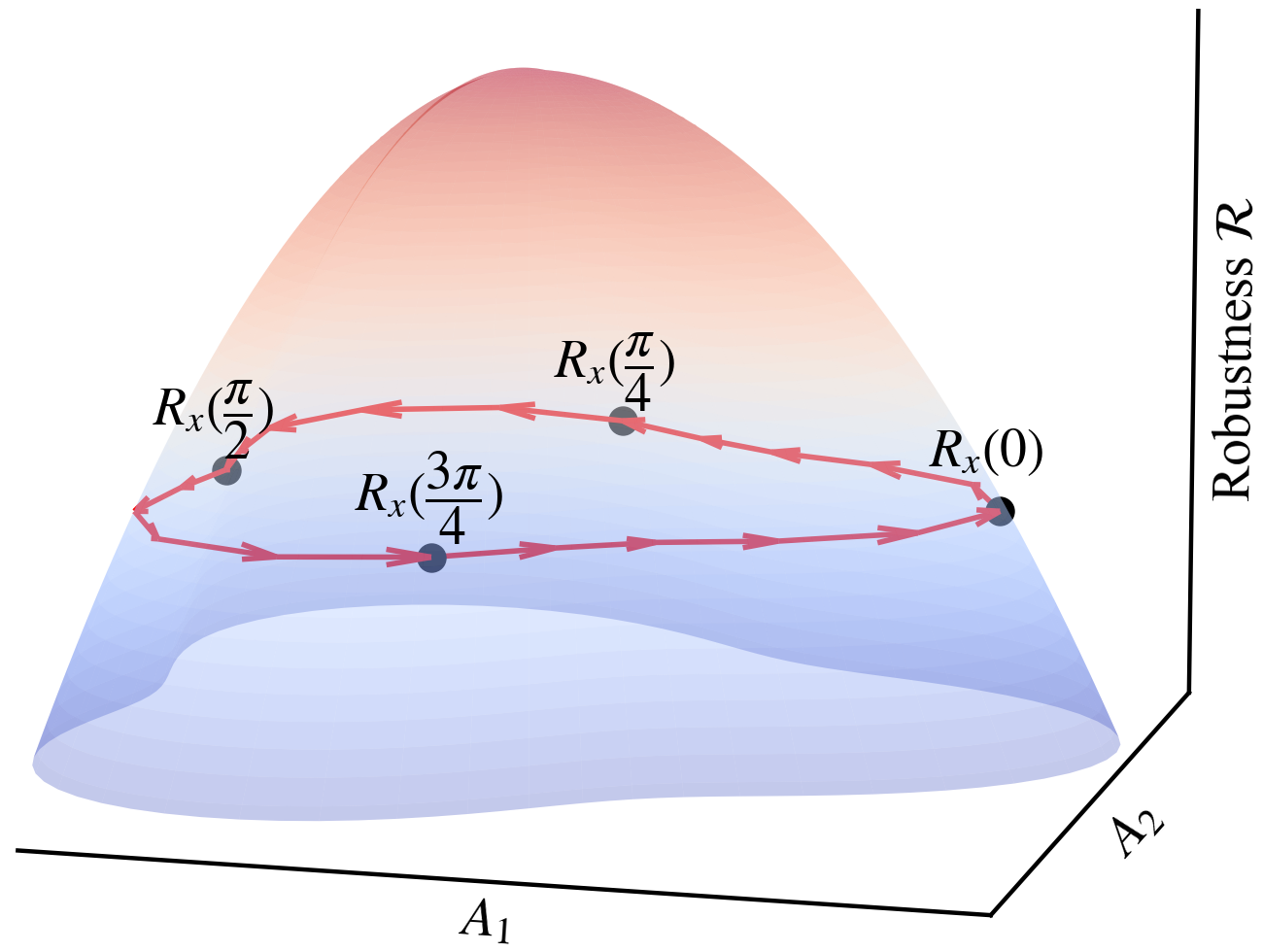
Figure 1: Schematic illustration of a level set exploration on a toy robustness landscape.

In the following sections, we present the mathematical formalism of the QCRL, introduce the RIPV algorithm, and provide numerical examples to demonstrate its effectiveness. We believe that this work opens new possibilities in the field of quantum control, offering a robust and flexible approach to pulse engineering in noisy quantum systems.

Advantages of our framework include:

• Unified description. In the QCRL, because it is defined independently from the control objective, we can consider all controllable objectives in a unified setting.

• Noise-centered perspective. The QCRL is defined by a noise model, rather than a control objective. It is a better mathematical tool for the NISQ era.

• Suitable for parametric gates. Using the RIPV algorithm, we can implement robust parametric gates with optimized control parameters.

• Generalizable algorithm design. In principle, the RIPV algorithm can be easily generalized to multi-qubit gates and more complex noise models.

• Decoupling multi-objectives. When dealing with multi-objective optimization, we can optimize one without undermining the others, effectively decoupling one objective from the others.

II Preliminaries

Our QCRL is built upon the two fields of QCL and robust quantum control, which we introduce briefly in this section.

II.1 Quantum control landscape

A landscape is the graph of a function or map. The study of landscapes focuses on problems that arise while optimizing this function, such as plateaus, local traps, etc. The concept of Quantum Control Landscapes (QCL) originates from the study of how quantum systems can be manipulated using external control fields to achieve specific objectives, such as high-fidelity quantum gates or precise state transfers. Herschel Rabitz and collaborators formalized the idea of QCL as a framework that maps control parameters (e.g., pulse amplitudes, phases, or durations) to an objective function, such as fidelity or population transfer. While other metrics, such as robustness, leakage, etc., are considered as constraints during the optimization on the QCL. This mapping creates a "landscape" in which the control parameters define the input space, and the output space is determined by the value of the objective function. The structure of this landscape is critical for understanding and optimizing quantum control.

The first property we would want in a QCL is the controllability of the quantum system. A quantum system is fully controllable if it can be steered to any desired state from any given initial state. Ramakrishna et al. [12] stated that an $N$-level system is fully controllable if the Lie algebra generated by the system and control Hamiltonians is $N^{2}$. Later, Schirmer et al. [13] examined controllability for single control pulses addressing multiple transitions, and Polack et al. [14] made a more subtle discussion by classifying uncontrollable systems into reducible and irreducible types. These foundational results established controllability as a cornerstone of QCL, ensuring that the optimization process has access to all necessary dynamical possibilities.

A key requirement for QCLs is the absence of local traps (i.e., local extrema) under ideal conditions, ensuring that gradient-based optimization algorithms converge to a global extremum of the objective function. Rabitz et al. [15] showed that, for controllable systems with unconstrained control fields, all local extrema are also global. However, this result holds only under specific conditions, notably the absence of constraints on the control fields and the fulfillment of controllability criteria.

Despite the idealized assumption of a trap-free landscape, the existence of local traps has been extensively studied. Rabitz initially formalized the distinction between global and local extrema in QCLs. Subsequent work by Pechen et al. [16] introduced the idea of kinematic and dynamic critical points, which can give rise to local traps. Commonly used QCLs are free of kinematic critical points, while dynamic critical points are more common and result from limitations in the control Hamiltonian or system dynamics. Studies by Wu et al. [17, 18] and Russell et al. [19] further analyzed the different types of critical points, providing a deeper understanding of the conditions under which traps might exist. For instance, constrained optimization in $SU(N)$ spaces, as demonstrated by Birtea et al. [20], revealed the presence of kinematic local extrema for $N\geq 5$. These findings highlight the importance of understanding the interplay between system dynamics, constraints, and the structure of the landscape. There have been controversies over whether the QCL is truly trap-free under realistic assumptions [21, 22, 23].

Beside those properties, the level sets of QCLs played an important role. A level set consists of all the control fields yielding the same value of the objective function. Level sets are especially useful for refining control solutions according to additional criteria. For example, the D-MORPH algorithm [24] and its unitary variant [25] allow for systematic exploration of level sets, enabling the optimization of secondary objectives such as gate time while maintaining transition probability or unitary gate. Pechen et al. [26] demonstrated that the level sets in two-level quantum systems are connected, further validating the efficacy of level set exploration algorithms for quantum control tasks. This ability to navigate level sets makes QCL a versatile framework for addressing multi-objective optimization problems in quantum systems.

In realistic applications, there are often multiple objectives such as fidelity, robustness, leakage, gate time, bandwidth and fluence, etc. In multi-objective optimization, there is no well-defined optimal solution. Rather, we care about the Pareto front, the set of optimized controls such that no objective can be further optimized without undermining another. Even if we cannot directly calculate the Pareto optimal solution, at least we want to iteratively update our solution towards the Pareto front as close as possible. Due to complexities in multi-objective optimization, people often use the aggregated objective function, such as taking the sum of all objectives in question. This aggregated objective makes the landscape complicated and unpredictable. Even worse, only having control over the aggregated objective means optimizing one could easily harm other objectives, thus never approaching the Pareto front. But if we can explore the level set of some landscape that we care the most, meanwhile optimizing some other criteria, we would finally have the hope to reach the Pareto front.

II.2 Robust quantum control

Robust quantum control is a vital discipline within quantum information science that focuses on maintaining the fidelity of quantum operations in the presence of various types of noise and uncertainties inherent in quantum systems. As quantum technologies advance, particularly in platforms such as superconducting qubits and solid-state spins [27, 28], the challenge of effectively managing noise—ranging from field (charge, flux, photon, etc.) fluctuations [29] to uncertain disturbances (crosstalk, unwanted couplings, etc.) [30, 31, 32] —has become increasingly critical. Robust quantum control techniques aim to design control protocols that can withstand these disturbances, ensuring reliable performance of quantum gates and operations. Methods such as dynamical decoupling [33], composite pulse sequences [34, 35], and advanced optimization strategies have been developed to enhance the resilience of quantum systems against noise [36, 37]. Furthermore, the introduction of a geometric framework for robust quantum control provides a powerful tool for visualizing and analyzing the robustness of quantum operations [10, 38, 39, 32]. This framework not only facilitates a deeper understanding of the landscape of control parameters but also aids in the systematic design of control strategies that can effectively mitigate the impact of generic noise [40].

III Quantum Control Robustness Landscape

We now define precisely what robustness means. We shall see that robustness can be defined for arbitrary types of noise, as long as it can be written as a Hamiltonian with stochastic parameters, which is a general enough condition. First, we take a look at what we are going to achieve from a toy model. Then, we define integral robustness and asymptotic robustness. Integral robustness, defined as the integral over the noise parameters, characterizes the system’s resilience to noise across all noise strengths. In contrast, asymptotic robustness, defined using a local expansion, describes the system’s response to noise at small noise strengths.

III.1 A first glance into QCRL

Enhancing the performance of quantum computers in the NISQ era towards error-corrected quantum computing can be logically decomposed into two primary tasks within the realm of quantum control: (1) increasing the fidelity of quantum operations, and (2) enhancing the robustness of these operations against noise. In this manuscript, we introduce a novel framework for the landscape of quantum control in the presence of noise, termed the Quantum Control Robustness Landscape (QCRL).

The key reason to study QCRLs is that traversing a level set (inputs that yield equal outputs) provides a series of equally robust controls. Unlike optimizing the QCL, essentially a fidelity landscape, where the peak represents control for a specific gate, a QCRL level set includes robust controls for different gates. This allows for finding multiple robust controls in a single run. Figure 1 illustrates this idea on a simple 2D toy landscape (which does not necessarily correspond to any realistic robustness model)

$$\mathcal{R} =-r^{2}$$

$$A_{1} =r\left(2+\cos^{2}3\theta/2\right)\cos\theta$$

$$A_{2} =r\left(2+\cos^{2}3\theta/2\right)\sin\theta\>,$$

where $\mathcal{R}$ represents the control’s robustness, $A_{1}$ and $A_{2}$ are control parameters. The red arrows represent the small steps that we take to vary the inputs $x$ and $y$ while maintaining $z=-16$ unchanged.

This toy landscape is unrealistically simple, since a 2D surface can only have 1D level sets which only allow movement in one direction. Real applications typically involve far more than two parameters, leading to higher-dimensional level sets and more complex traversal paths. As a result, Figure 1 gives a wrong intuition that a path in a level set should be a closed loop, which is far from true in higher-dimensional level sets. Therefore, usually in the parameter space, the point for $R_{x}(0)$ does not overlap with $R_{x}(2\pi)$. With extra dimensions, we can choose a path in a higher-dimensional level set so that the path encompasses all the gates we want to be robust.

To rigorously define QCRL, we propose a quantitative and general definition of quantum control robustness. We then present the mathematical formalism of QCRL and elucidate several key concepts. Additionally, we briefly explore potential applications of QCRL in quantum computing.

III.2 Integral Robustness

III.2.1 Notations

First of all, we introduce a useful notation of propagator that allows us to deal with time-dependent and time-independent Hamiltonians at once. Note that throughout this paper, we set $\hbar=1$.

Notation 1.

Let’s denote by $U^{H}(t)$ the propagator generated by a (whether time-dependent or time-independent) Hamiltonian $H$ in the time period $[0,t]$.

In a more common notation, for a time-independent Hamiltonian $H$, we have $U^{H}(t)=e^{-iHt}$, and for a time-dependent $H(t)$, we have $U^{H}(t)=U^{H(\tau)}(t)=\mathcal{T}e^{-i\int_{0}^{t}H(\tau)\differential{\tau}}$ with $\mathcal{T}$ being the time-ordering operator. Pay attention to $\tau$ in the exponent of our notation $U^{H(\tau)}(t)$. It is only used to indicate we are dealing with a time-dependent Hamiltonian, and is essentially the variable of integration in the formal exponent $\int_{0}^{t}H(\tau)\differential{\tau}$.

Throughout this paper, we assume a system dictated by Hamiltonian

$$H=H_{\text{s}}+H_{\text{c}}+H_{\text{n}}\>,$$

with $H_{\text{s}}$ the system Hamiltonian, $H_{\text{c}}$ the control Hamiltonian, $H_{\text{n}}$ the noise Hamiltonian introducing stochastic perturbations. We omit the explicit time variable in $H_{\text{n}}$ and $H_{\text{c}}$ to emphasize the entire map, rather than a specific instance of $H_{\text{n}}(t)$ at any given $t$. Upon fixing a coordinate frame and time $t$, $H_{\text{n}}(t)$ is represented as a matrix. Let’s denote by $\mathcal{H}_{\text{n}}$ the set of matrices from which the instant noise operator $H_{\text{n}}(t)$ might take value. It is a subalgebra of $n\times n$ Hermitian matrices. Subsequently, $H_{\text{n}}:t\mapsto H_{\text{n}}(t)$ represents a map residing within the exponential set

$${\mathcal{H}_{\text{n}}}^{[0,T]}:=\{\text{continuous }H_{\text{n}}:[0,T]\to\mathcal{H}_{\text{n}}\}\>,$$ (1)

i.e. the set of all continuous maps from $[0,T]$ to $\mathcal{H}_{\text{n}}$. If we view $\mathcal{H}_{\text{n}}$ as a linear space of dimension $n^{2}$, then the image of the continuous map $H_{\text{n}}$ is a path (strictly speaking, a bounded 1D submanifold) when time evolves from $0$ to $t$. In this way, ${\mathcal{H}_{\text{n}}}^{[0,T]}$ can be viewed as a space of paths, where each $H_{\text{n}}$ is a path in $\mathcal{H}_{\text{n}}$. In the following discussions, we will use “path” as a synonym of “time-dependent noise operator”.

III.2.2 Path integral perspective

In this part of the discussion, we are going to see that what we need for defining a general robustness metric is mathematically a path integral. We will start from a intuitive construction and work our way to a rigorous definition.

To understand the system’s robustness to stochastic noise, we must take into account all possible noise operators in ${\mathcal{H}_{\text{n}}}^{[0,T]}$ when examining the system’s performance. In other words, we might need to evaluate an expression in the form of $\int J[H_{\text{n}}]\,\differential{H_{\text{n}}}$, where $J:{\mathcal{H}_{\text{n}}}^{[0,T]}\to\mathbb{R}$ is some functional of $H_{\text{n}}$ that assesses the system’s performance.

Since $H_{\text{n}}$ is a path as we discussed in the end of the previous section, mathematically speaking, $\int J[H_{\text{n}}]\,\differential{H_{\text{n}}}$ is a form of path integral. It is fundamentally different from ordinary integrals over $\mathbb{R}^{n}$. A common mistake is to write $\differential{H_{\text{n}}}=\partialderivative{H_{\text{n}}(t)}{t}\differential{t}$, wrongly treating it as integrating over all instant Hamiltonians $H_{\text{n}}(t)$. This is incorrect because we are integrating over all paths $H_{\text{n}}$, instead of matrices $H_{\text{n}}(t)$. To see it from another perspective, $J[H_{\text{n}}]$, as a functional of $H_{\text{n}}$, does not make sense when we ask the value of $J$ at a specific time $t$, not to mention integrating it over $t$. To make the integral well-defined, the differential $\differential{H_{\text{n}}}$ should be the measure of a neighborhood of $H_{\text{n}}$. In other words, we need a measure on the space ${\mathcal{H}_{\text{n}}}^{[0,T]}$. To emphasize its contrast to the “ordinary” measure $\differential{x}$, we denote this measure of paths with $\DD{H_{\text{n}}}$. To summarize, we want to define a path integral of the form

$$\int_{H_{\text{n}}\in{\mathcal{H}_{\text{n}}}^{[0,T]}}J[H_{\text{n}}]\DD{H_{\text{n}}}\>.$$

To compute the path integral, it is imperative to first define a measure $\mu$ on the space of paths ${\mathcal{H}_{\text{n}}}^{[0,T]}$, or equivalently the space of maps. Defining a measure in such a space poses significant challenges owing to its large cardinality (size of an infinite set). Nevertheless, for practical scenarios, a parametrization of $H_{\text{n}}$ induces a measure on ${\mathcal{H}_{\text{n}}}^{[0,T]}$.

Let’s see how the measure on ${\mathcal{H}_{\text{n}}}^{[0,T]}$ can be induced by the measure of $\mathbb{R}^{n}$. Once we parameterize the noise Hamiltonian $H_{\text{n}}$ by $\mathbf{B}\in\mathbb{R}^{n}$, formally

$$H_{\text{n}}(t)=H_{\text{n}}(t;\mathbf{B})\>,$$

we get a map from parameters to paths, $H_{\text{n}}:\mathbb{R}^{n}\to{\mathcal{H}_{\text{n}}}^{[0,T]}$. Intuitively, it is indeed such a map because a parameter vector $\mathbf{B}$ defines a time-dependent noise operator in ${\mathcal{H}_{\text{n}}}^{[0,T]}$. To be more strict, contemplate the notation $H_{\text{n}}(\_;\mathbf{B})$ where $\mathbf{B}$ is fixed but $t$ is to be determined. It defines a path in ${\mathcal{H}_{\text{n}}}$, because whenever we insert a time instant $t$, we get a matrix in $\mathcal{H}_{\text{n}}$ (see definition in Equation 1). Therefore, $H_{\text{n}}$ is such a map that when we feed a parameter vector $\mathbf{B}\in\mathbb{R}^{n}$, we get a path $H_{\text{n}}(\_;\mathbf{B})\in{\mathcal{H}_{\text{n}}}^{[0,T]}$. Moving on to subsets, if $\mathcal{B}\subset\mathbb{R}^{n}$ is a measurable neighborhood of $\mathbf{B}$, we can denote by $H_{\text{n}}(\_;\mathcal{B})\subset{\mathcal{H}_{\text{n}}}^{[0,T]}$ the subset of operators parameterized by all $\mathbf{B}\in\mathcal{B}$, the measure of $H_{\text{n}}(\_;\mathcal{B})$ is thus defined as

$$\mu\big{(}H_{\text{n}}(\_;\mathcal{B})\big{)}:=\mu_{L}(\mathcal{B})\>,$$ (2)

where $\mu_{L}(\mathcal{B})$ denotes the Lebesgue measure of $\mathbb{R}^{n}$. In other words, when we calculate the path integral, we convert back to $\mathbb{R}^{n}$ as

$$\int J[H_{\text{n}}]\DD{H_{\text{n}}}:=\int J[H_{\text{n}}(\_;\mathbf{B})]\differential{\mathbf{B}}\>.$$ (3)

In this manner, we have defined a measure and therefore the integral on the parametrizable subset of $\mathcal{H}_{\text{n}}^{[0,T]}$, though lacking some mathematical rigor. Let’s check these issues.

1. Symmetric treatment on parameters. By using a rotational symmetric measure in $\mathbb{R}^{n}$, we presume subjectively, that each component $B_{i}$ in vector $\mathbf{B}$ has equal influence on $H_{\text{n}}$. To allow different effects $B_{i}$ has on $H_{\text{n}}$, we need a Jacobian-like coefficient. This is addressed by inserting a probability function in the formal definition, writing down something like $\int J[H_{\text{n}}]p(H_{\text{n}})\DD{H_{\text{n}}}$.

2. Additivity. To ensure the induced measure to be additive, two sufficient conditions should be posited: (1) the map $H_{\text{n}}$ is continuous over both $t$ and $\mathbf{B}$; (2) the map $H_{\text{n}}:\mathbb{R}^{n}\to{\mathcal{H}_{\text{n}}}^{[0,T]}$ acts as a bijection nearly everywhere, with the exception of a null set (a subset of zero measure). Given these sufficient conditions, we can ascertain that

   $$\mu\big{(}H_{\text{n}}(\_;\mathcal{B}_{1})\big{)}+\mu\big{(}H_{\text{n}}(\_;\mathcal{B}_{2})\big{)}$$

   $$=\mu\big{(}H_{\text{n}}(\_;\mathcal{B}_{1}\cup\mathcal{B}_{2})\big{)}\>,$$

   and the induced measure is thus well defined.

3. Invariance under frame transformation. It is noteworthy that the measure $\mu(H_{\text{n}})$ should remain invariant under the transformation of any frame $U(t)$. However, addressing the property of invariance proves to be challenging, and consequently, computations are typically executed numerically within a fixed coordinate frame.

To summarize, by defining the measure of $H_{\text{n}}(\_;\mathcal{B})$ to be the measure in $\mathcal{B}$ as in Equation 2, we can safely replace $\DD{H_{\text{n}}}$ by $\differential{\mathbf{B}}$ as in Equation 3. Keep in mind that this replacement does not introduce the Jacobian in the way $\DD{H_{\text{n}}}=\absolutevalue{\partialderivative{H_{\text{n}}}{\mathbf{B}}}\differential{\mathbf{B}}$, because, as we discussed earlier, $\DD$ is the measure of the path rather than the differential of the matrix $H_{\text{n}}(t;\mathbf{B})$.

Given a well-defined differential $\DD{H_{\text{n}}}$, it is reasonable to further postulate that the noise adheres to a probability distribution characterized by the density function $p(H_{\text{n}})$. Consequently, the probability that the noise resides within a small neighborhood around $H_{\text{n}}$ is denoted by $p(H_{\text{n}})\DD{H_{\text{n}}}$. In numerical computations, the specific probability of a time-dependent Hamiltonian is frequently unknown; however, we can hypothesize the probability distribution of the noise parameters. Therefore, it becomes feasible to substitute $p(H_{\text{n}})$ with $p(\mathbf{B})$ and perform integration over $\mathbf{B}$. Equipped with these methodologies, we can formally characterize the robustness of a control with respect to the system’s noise. In the subsequent definition, temporal dependence is presumed throughout, yet omitted for clarity unless explicitly necessary.

III.2.3 Formal definition

Definition 1 (Robustness).

Given a control $H_{\text{c}}(t)$ applied to this system, the control’s robustness $\boxed{\mathcal{R}[H_{\text{c}}]}$ with respect to a specific subset of noise Hamiltonians $\mathcal{H}_{\text{n}}$ is defined as the mathematical expectation of the average gate fidelity between the noiseless propagator $U_{\text{sc}}=U^{H_{\text{s}}+H_{\text{c}}}(T)$ and the actual noisy propagator $U_{\text{scn}}=U^{H_{\text{s}}+H_{\text{c}}+H_{\text{n}}}(T)$. Mathematically,

$$\mathcal{R}[H_{\text{c}}]:=\int_{\mathrlap{\raisebox{0.0pt}{${}_{H_{\text{n}}\in{\mathcal{H}_{\text{n}}}^{[0,T]}}$}}}\qquad F\big{(}U_{\text{sc}}(T),U_{\text{scn}}(T)\big{)}\,p(H_{\text{n}})\DD{H_{\text{n}}}\>,$$ (4)

where $p(H_{\text{n}})$ is non-zero only at the noise operators that might affect the system. If we only consider noise operators parametrizable by $\mathbf{B}$, and denote $U_{\text{scn}}(T;\mathbf{B})=U^{H_{\text{s}}+H_{\text{c}}+H_{\text{n}}(\tau;\mathbf{B})}(T)$

$$\mathcal{R}[H_{\text{c}}]:= \int_{\mathbf{B}\in\mathbb{R}^{n}}F\big{(}U_{\text{sc}}(T),U_{\text{scn}}(T;\mathbf{B})\big{)}\,p(\mathbf{B})\differential{\mathbf{B}}\>.$$ (5)

Based on the definition of fidelity, what we defined here is a number $0\leq\mathcal{R}\leq 1$. In the following text, we occasionally refer to such $\mathcal{R}[H_{\text{c}}]$ as the integral robustness to distinguish it from the more practical $n$-th order asymptotic robustness that is to be introduced.

Remark 1.

It is important to highlight that this definition is NOT an “average of fidelity” in the conventional sense, as fidelity typically involves a comparison between the realistic propagator $U_{\text{ideal}}$. In contrast, robustness is determined by comparing the noiseless propagator $U_{\text{sc}}$ with the noisy propagator $U_{\text{scn}}$. Robustness $\mathcal{R}$ is influenced exclusively by two competing factors: the noise $H_{\text{n}}$ that generates errors and the control $H_{\text{c}}$ employed to suppress these errors.

Remark 2.

It should be observed that complete robustness can be more directly defined via the probability and measurement of the parameters pertaining to the noise operator. Nonetheless, the measurement of functions does not necessarily have to be derived from these parameters; hence, it has been conceptualized through the measure on the space of paths ${\mathcal{H}_{\text{n}}}^{[0,T]}$. Should a more generalized measure be introduced, this definition of robustness could be further refined and rendered more rigorous.

III.2.4 Error evolution

Transitioning to the interaction picture with respect to the noiseless propagator $U_{\text{sc}}(t)=U^{H_{\text{s}}+H_{\text{c}}(\tau)}(t)$ reveals that, while the noise itself cannot be directly controlled, the accumulation of errors induced by the noise can be effectively suppressed through the application of control fields. These control fields influence the manner in which errors accumulate over time, thereby providing a mechanism to mitigate their impact. By analyzing the error evolution in the interaction picture, we can simplify and formalize the definition of robustness. In this framework, the noise Hamiltonian transforms as:

$$H_{\text{n}}^{\text{sc}}(t) =U^{-H_{\text{s}}-H_{\text{c}}(\tau)}(t)\cdot H_{\text{n}}(t)\cdot U^{H_{\text{s}}+H_{\text{c}}(\tau)}(t)$$ (6)

$$=U_{\text{sc}}^{\dagger}H_{\text{n}}U_{\text{sc}}^{\vphantom{\dagger}}\>.$$ (7)

Notably, the noise operator $H_{\text{n}}$ may exhibit either time-dependent or time-independent characteristics, a distinction that is irrelevant in our discussion.

Definition 2 (Error evolution).

The error evolution or error propagator is defined as the unitary evolution

$$U_{\text{n}}^{\text{sc}}(t)=U^{H_{\text{n}}^{\text{sc}}(\tau)}(t)=U^{U_{\text{sc}}^{\dagger}H_{\text{n}}U_{\text{sc}}}(t)\>,$$

where $H_{\text{n}}^{\text{sc}}$ is the noise Hamiltonian under the interaction picture. $U_{\text{n}}^{\text{sc}}(T)=I$ means error is canceled exactly at time $T$.

Remark 3 (Integral robustness by error evolution).

With the definition of error evolution and the interaction picture, the fidelity between $U_{\text{sc}}$ and $U_{\text{scn}}$ becomes,

$$\hphantom{{}={}}F\big{(}U_{\text{sc}}(T),U_{\text{scn}}(T)\big{)}$$

$$=\Tr\big(U_{\text{sc}}^{\dagger}(T)\cdot U_{\text{scn}}(T)\big{missing})/d$$

$$=\Tr\big(U_{\text{sc}}^{\dagger}(T)\cdot U_{\text{sc}}(T)\cdot U_{\text{n}}^{\text{sc}}(T)\big{missing})/d$$

$$=\Tr\big(U_{\text{n}}^{\text{sc}}(T)\big{missing})/d$$

$$=F\big{(}U_{\text{n}}^{\text{sc}}(T),\mathrm{I}\big{)}\>,$$

where $d$ is the dimension of the Hilbert space. Hence, the integral robustness can also be written as

$$\mathcal{R}[H_{\text{c}}] =\int_{H_{\text{n}}\in{\mathcal{H}_{\text{n}}}^{[0,T]}}\frac{1}{d}\Tr\big(U_{\text{n}}^{\text{sc}}(T)\big{missing})p(H_{\text{n}})\DD{H_{\text{n}}}$$ (8)

$$=\int_{H_{\text{n}}\in{\mathcal{H}_{\text{n}}}^{[0,T]}}F(U_{\text{n}}^{\text{sc}}(T),I)p(H_{\text{n}})\DD{H_{\text{n}}}\>.$$ (9)

This expression coheres with our intuition that, within the interaction picture, a robust system characterized by a larger $\mathcal{R}$ should exhibit an error evolution $U_{\text{n}}^{\text{sc}}$ that closely resembles the identity evolution $I$. Fundamentally, the robustness of a system is encapsulated in the error evolution $U_{\text{n}}^{\text{sc}}$.

III.3 Asymptotic robustness

While the integral robustness is elegant in both construction and interpretation, it is impractical, as it requires simulating for fidelity under all possible noise operators. Instead, we can take a more practical approach by focusing on robustness to small noise. In this section, we define asymptotic robustness metrics that capture the system’s resilience as the noise strength approaches zero.

Let’s first look at a simpler case, where $H_{\text{n}}=\delta H_{\text{n},0}$ is quasi-static noise, with $\delta$ an unknown constant.

$$H_{\text{n}}^{\text{sc}}(t) =U^{-H_{\text{s}}-H_{\text{c}}(\tau)}(t)\cdot\delta H_{\text{n},0}\cdot U^{H_{\text{s}}+H_{\text{c}}(\tau)}(t)$$

$$=\delta U_{\text{sc}}^{\dagger}(t)H_{\text{n},0}U_{\text{sc}}^{\vphantom{\dagger}}(t)\>.$$

The error evolution is $U_{\text{n}}^{\text{sc}}=U^{H_{\text{n}}^{\text{sc}}}(t)=U^{\delta U_{\text{sc}}^{\dagger}H_{\text{n},0}U_{\text{sc}}^{\vphantom{\dagger}}}(t)$. Since noise should be relatively small compared to control field strength, we can assume $\delta$ is very small. Then the error evolution is approximately, to the first order,

$$U_{\text{n}}^{\text{sc}}(T) =\mathcal{T}e^{-i\int_{0}^{T}\delta U_{\text{sc}}^{\dagger}(\tau)H_{\text{n},0}U_{\text{sc}}^{\vphantom{\dagger}}(\tau)\differential{\tau}}$$

$$\approx I-i\delta\int_{0}^{T}U_{\text{sc}}^{\dagger}(\tau)H_{\text{n},0}U_{\text{sc}}^{\vphantom{\dagger}}(\tau)\differential{\tau}\>.$$

Then the overlap between $U_{\text{n}}^{\text{sc}}$ and $I$ all boils down to the norm of the matrix integral $\int_{0}^{T}U_{\text{sc}}^{\dagger}(\tau)H_{\text{n},0}U_{\text{sc}}^{\vphantom{\dagger}}(\tau)\differential{\tau}$. The value of $\mathcal{R}$ is mainly determined by the matrix value when $\delta$ is small enough. We can generalize this quantity to higher orders.

In general, by using tools like the Magnus expansion or high order derivatives, we can define another type of asymptotic robustness that holds in the limit of $\delta\to 0$, where $\delta$ is the strength of some noise (not necessarily the strength of quasi-static noise).

Example 1 ($n$-th order robustness by Magnus expansion).

In previous example, we have shown that the robustness can be calculated by $\mathcal{R}[H_{\text{c}}]=\int_{H_{\text{n}}}\Tr(U_{\text{n}}^{\text{sc}})/d\DD{H_{\text{n}}}$. Furthermore, we can use Magnus expansion to get a more useful quantity:

$$U_{\text{n}}^{\text{sc}}= U^{H_{\text{n}}^{\text{sc}}}(T)$$

$$=$$

$$= \exp\left(-i\delta M_{1}(T)-\frac{1}{2}\delta^{2}M_{2}(T)+O(\delta^{3})\right)\>,$$

where $M_{k}$ denotes the $k$-th order term in the Magnus expansion. The 1st-order term $M_{1}$ tells us, to the 1st order, the amount of error induced by a unit of noise (i.e. $\delta=1$) under the amplification or suppression of the control. We refer to its norm as the 1st-order noise susceptibility $\mathcal{S}^{1}_{\text{(M)}}$:

$$\mathcal{S}^{1}_{\text{(M)}}=\norm{M_{1}(T)}=\norm{\int_{0}^{T}\frac{H_{\text{n}}^{\text{sc}}(t)}{\delta}\differential{t}}\>.$$ (10)

The subscript $\square_{\text{(M)}}$ indicates it is defined by the Magnus expansion, and will be omitted when the context is clear. We always assume this Magnus-expansion-based definition throughout this paper. Similarly, we can define the 2nd-order noise susceptibility:

$$\mathcal{S}^{2}_{\text{(M)}} =\norm{M_{2}(T)}$$ (11)

$$=\norm{\int_{0}^{T}\left[\frac{H_{\text{n}}^{\text{sc}}(t)}{\delta},\int_{0}^{t}\frac{H_{\text{n}}^{\text{sc}}(\tau)}{\delta}\differential{\tau}\right]\differential{t}}\>.$$ (12)

Naturally, we define $n$-th order noise susceptibility as

$$\mathcal{S}^{n}_{\text{(M)}}=\norm{M_{n}(T)}\>.$$

Because we only care about its relative magnitude, the norms used here can be any norm, as long as it bounds every component of the matrix. For example, any element-wise $p$-norm works fine, but trace norm is unfavorable since it does not bound off-diagonal components.

However, the definitions of $\mathcal{S}^{n}$ are dependent on gate time $T$ and $n$ (the order of $\delta$). Another drawback is that $\mathcal{S}^{n}$ is negatively correlated with the control’s robustness. Hence, from the definitions of $n$-th order noise susceptibilities $\mathcal{S}^{n}$, we can define the $n$-order robustness $\mathcal{R}^{n}$. To get rid of the relation to $T$ and $n$, we take the $n$-th root and then divide it by $T$, which gives $\frac{\sqrt[n]{\mathcal{S}^{n}}}{T}$. To make this quantity positively correlated to robustness, we take its reciprocal. We finally take logarithm of base 10 to make the numbers compact and to manifest the order of error suppression. In summary, we define $n$-th order robustness (by Magnus expansion) as

$$\mathcal{R}^{n}_{\text{(M)}} =\log_{10}\left({\frac{T}{\sqrt[n]{\mathcal{S}^{n}_{\text{(M)}}}}}\right)$$

$$=\log_{10}T-\frac{1}{n}\log_{10}\mathcal{S}^{n}_{\text{(M)}}\>.$$

This robustness is more intuitive, but it could exceed the computer precision when $\mathcal{S}^{n}\to 0$, though this hardly happens in realistic applications. Since the robustness and susceptibility are monotonically related, we mainly use susceptibility in this paper for its computational simplicity.

Example 2 ($n$-th order robustness by derivatives).

We can also define asymptotic noise susceptibility by higher derivatives.

$$\mathcal{S}^{n}_{\text{(D)}} =\norm{\partialderivative[n]{U_{\text{n}}^{\text{sc}}}{\delta}}\>.$$

And we define asymptotic robustness by derivatives similarly,

$$\mathcal{R}^{n}_{\text{(D)}} =\log_{10}T-\frac{1}{n}\log_{10}\mathcal{S}^{n}_{(D)}\>.$$

Note that the 1st-order noise susceptibility defined by either derivatives or the Magnus expansion is the same, but they disagree on higher order susceptibilities (hence also on robustness):

$$\partialderivative{U_{\text{n}}^{\text{sc}}}{\delta}=-M_{1} \Rightarrow\mathcal{S}^{1}_{\text{(D)}}=\mathcal{S}^{1}_{\text{(M)}}$$

$$\partialderivative[2]{U_{\text{n}}^{\text{sc}}}{\delta}=-\frac{1}{2}M_{1}^{2}+iM_{2} \Rightarrow\mathcal{S}^{2}_{\text{(D)}}\leq\frac{1}{2}\left(\mathcal{S}^{1}_{(D)}\right)^{2}\!+\mathcal{S}^{2}_{\text{(M)}}\>,$$

where $M_{k}$ is a shorthand for $M_{k}(T)$ in the Magnus expansion at time $T$.

The two definitions of asymptotic robustness are essentially equivalent. If the lower-than-$n$-th order susceptibilities all vanish, then these two definitions of susceptibility (or robustness) coincide within a constant at $n$-th order. Precisely,

$$\mathcal{S}^{k}_{\text{(D)}}=\mathcal{S}^{k}_{\text{(M)}}=0\quad\forall k=1,\dots,n-1,$$

$$\Longrightarrow\quad \mathcal{S}^{n}_{\text{(D)}}\propto\mathcal{S}^{n}_{\text{(M)}}\>.$$

Particularly, it becomes trivial for noise susceptibility on the 1st order, which we simply denote by $\mathcal{S}^{1}$ (and the robustness by $\mathcal{R}^{1}$):

$$\mathcal{S}^{1}:=\mathcal{S}^{1}_{\text{(D)}}=\mathcal{S}^{1}_{\text{(M)}}\>.$$

Example 3 (Multiple noise sources).

If there are more than one noise sources, i.e. $H_{\text{n}}=\sum_{k}H_{\text{n},k}$ where each $H_{\text{n},k}$ is an independent quasi-static noise, we can easily find out that the 1st-order term in the Magnus expansion for noise $H_{\text{n}}$ is simply the sum of that for $H_{\text{n},k}$ ,

$$M_{1}(T;H_{\text{n}})=\int_{0}^{T}\frac{\sum_{k}H_{\text{n},k}^{\text{sc}}(t)}{\delta}\differential{t}=\sum_{k}M_{1}(T;H_{\text{n},k})\>.$$

Then, by the triangle inequality of matrix norms, the 1st-order noise susceptibility is bounded by the sum

$$\norm{M_{1}(T;H_{\text{n}})}=\mathcal{S}^{1}[H_{\text{n}}]$$

$$\leq\sum_{k}\mathcal{S}^{1}[H_{\text{n},k}]=\sum_{k}\norm{M_{1}(T;H_{\text{n},k})}\>.$$

Thus, the first-order robustness concerning a single noise source can be readily extended to encompass multiple noise sources. Higher-order robustness could similarly be generalized to the scenario involving multiple noise sources; however, this would entail a remarkably complex array of mixed products of different $H_{\text{n},k}$’s. Consequently, such formulations are not presented here.

Remark 4 (Comparison to optimization on QCL).

In QCL, our objective is either the state fidelity, the gate fidelity, or the expectation of an observable $\mathcal{O}$. The objective is always a function of the final time propagator $U_{\text{sc}}(T)$, with $\eta$ being the ideal final state and $G$ being the ideal gate,

$$F_{\text{state}} =\Big{(}\Tr\sqrt{\sqrt{\eta}U_{\text{sc}}(T)\rho_{0}U_{\text{sc}}^{\dagger}(T)\sqrt{\eta}}\Big{)}^{2}\>,$$

$$F_{\text{gate}} =\Tr\left(U_{\text{sc}}^{\dagger}(T)G\right)\>,$$

$$\expectationvalue{\mathcal{O}} =\Tr\left(U_{\text{sc}}^{\dagger}(T)\mathcal{O}U_{\text{sc}}^{\vphantom{\dagger}}(T)\right)\>.$$

On the other hand, in QCRL, if we optimize the 1st-order susceptibility $\mathcal{S}^{1}$, our objective is an integral over all propagators $U_{\text{sc}}(t)$ for $t\in[0,T]$, which is

$$\mathcal{S}^{1} =\norm{\int_{0}^{T}\frac{H_{\text{n}}^{\text{sc}}(t)}{\delta}\differential{t}}$$

$$=\norm{\int_{0}^{T}U_{\text{sc}}^{\dagger}(t)H_{\text{n},0}U_{\text{sc}}^{\vphantom{\dagger}}(t)\differential{t}}\>.$$

Notice the difference in $U_{\text{sc}}(t)$ and $U_{\text{sc}}(T)$. We can tell by these definitions that the landscape of noise susceptibility (hence also robustness) is fundamentally different from that of the fidelity-based QCLs.

III.4 Breakdown of QCRL

As elucidated previously, QCL defines the map from control parameters to the fidelity of the ideal quantum gate. Since now a measure is defined as Equation 4, there emerges a novel landscape distinct from QCL, which facilitates the characterization of quantum control performance, particularly with respect to robustness.

Hereinafter, we suppose the control Hamiltonian is parameterized by a vector $\mathbf{A}\in\mathbb{R}^{n}$, formally

$$H_{\text{c}}(t)=H_{\text{c}}(t;\mathbf{A})\>.$$

Definition 3 (QCRL).

The QCRL is defined as the map $\mathcal{R}:\mathbf{A}\mapsto\mathcal{R}(\mathbf{A})$ from control parameters $\mathbf{A}$ to the control’s robustness $\mathcal{R}$ against certain noise types.

In practical quantum systems, reference $\mathbf{A}$ typically pertains to the parameters of control fields, which include waveforms of electronic or magnetic fields, as well as the envelope and frequency of microwave fields, among others. In this work, we assume the general form of control

$$H_{\text{c}}(t;\mathbf{A}) :=\sum_{k}\Omega_{k}(t;\mathbf{A})H_{\text{c},k},$$

where time-dependence are reflected in $\Omega_{k}(t)$ and $H_{\text{c},k}$ are time-independent operators. We will refer to $\Omega_{k}(t)$ as pulses, which are not necessarily the physically applied pulse signals.

Remark 5 (Decomposition of QCRL).

If we look into this $\mathcal{R}(\mathbf{A})$, it is actually composed of the following maps. In this paper, we use $[\dots]$ to denote functional dependence, and $(\dots)$ to denote time dependence.

1. A vector of maps $\vec{\Omega}=\{\Omega_{k}\}_{k}$ from control parameters $\mathbf{A}$ to control pulses $\Omega_{k}(t;\mathbf{A})$, each corresponding to one of the control terms $H_{\text{c},k}$. Each $\Omega_{k}(\mathbf{A})$ is a function of $t$, denoted by $\Omega_{k}(t;\mathbf{A})$:

   $$\Omega_{k}:\mathbf{A} \mapsto\Omega_{k}(\mathbf{A}),$$

   $$\text{s.t. }\Omega_{k}(\mathbf{A})(t) =\Omega_{k}(t;\mathbf{A})\>.$$

2. A map $H_{\text{c}}$ from those time-dependent coefficients $\Omega_{k}$ to a control Hamiltonian $H_{\text{c}}[\vec{\Omega}]$, where $H_{\text{c}}[\vec{\Omega}]$ is a time-dependent operator:

   $$H_{\text{c}}:\vec{\Omega} \mapsto H_{\text{c}}[\vec{\Omega}],$$

   $$\text{s.t. }H_{\text{c}}[\vec{\Omega}](t) =\sum_{k}\Omega_{k}(t)H_{\text{c},k}\>.$$

3. A map $U_{\text{sc}}$ from control Hamiltonian $H_{\text{c}}$ to the noiseless propagator $U_{\text{sc}}[H_{\text{c}}]$, where $U_{\text{sc}}[H_{\text{c}}]$ is a time-independent operator:

   $$U_{\text{sc}}:H_{\text{c}} \mapsto U_{\text{sc}}[H_{\text{c}}],$$

   $$\text{s.t. }U_{\text{sc}}[H_{\text{c}}](t) =U^{H_{\text{s}}+H_{\text{c}}(\tau)}(t)\>.$$

4. A map from the propagator $U_{\text{sc}}(t)$ to any metric of robustness $\mathcal{R}$ (integral robustness, asymptotic robustness, etc.):

   $$\mathcal{R}:U_{\text{sc}}\mapsto\mathcal{R}[U_{\text{sc}}]\>.$$

Finally, we get the robustness map from control parameters $\mathbf{A}$ to some metric of robustness $\mathcal{R}$ by composing all the maps,

$$\mathcal{R}:\mathbf{A}\mapsto\vec{\Omega}(\mathbf{A})\mapsto H_{\text{c}}[\vec{\Omega}]\mapsto U_{\text{sc}}[H_{\text{c}}]\mapsto\mathcal{R}[U_{\text{sc}}(\mathbf{A})]\>.$$ (13)

If we write out the time dependence explicitly, the map then looks like

$$\mathcal{R}: \mathbf{A}\xmapsto{\vec{\Omega}}\{\Omega_{k}(t;\mathbf{A})\}_{k}\xmapsto{H_{\text{c}}}\sum_{k}\Omega_{k}(t;\mathbf{A})H_{\text{c},k}$$

$$\xmapsto{U_{\text{sc}}}U^{H_{\text{s}}+\sum_{k}\Omega_{k}(\tau;\mathbf{A})H_{\text{c},k}}(t)\xmapsto{\mathcal{R}}\mathcal{R}[U_{\text{sc}}]\>.$$

Among the four maps above, only the first one $\vec{\Omega}$ is a function of numbers, i.e. the control parameters $\mathbf{A}$. The second map $H_{\text{c}}$ maps the functions $\vec{\Omega}(t)$ to a time-dependent Hamiltonian $H_{\text{c}}(t)$. The rest two maps, $U_{\text{sc}}$ and $\mathcal{R}$, have either time-ordered exponential or integrals. So they are all functionals that depend on the whole input functions defined on the time interval $[0,T]$. This decomposition into four maps will aid us in further discussions on topics such as critical points.

Remark 6 (Functional dependence on $U_{\text{n}}^{\text{sc}}$).

We have assumed in previous discussions that the robustness $\mathcal{R}$ is always a functional of the trajectory of the propagator $U_{\text{sc}}(t)$, i.e. they depend on all the values of $U_{\text{sc}}(t)$ on $t\in[0,T]$. Let’s check that the definitions of robustness we have defined before always fit this assumption. The integral robustness is defined as

$$\mathcal{R}[U_{\text{sc}}] =\int_{H_{\text{n}}\in\mathcal{H}_{\text{n}}}F(U_{\text{n}}^{\text{sc}},I)p(H_{\text{n}})\differential{H_{\text{n}}}$$

$$=\int_{H_{\text{n}}\in\mathcal{H}_{\text{n}}}F\left(U^{U_{\text{sc}}^{\dagger}(\tau)H_{\text{n}}U_{\text{sc}}^{\vphantom{\dagger}}(\tau)}(T),I\right)\;p(H_{\text{n}})\differential{H_{\text{n}}}\>.$$

Hence the integral robustness is indeed a functional of $U_{\text{sc}}(t)$. If the noise is quasi-static noise, then the first order robustness $\mathcal{R}^{1}$ is, too. Here we only check the noise susceptibility $\mathcal{S}^{1}$ is a functional of $U_{\text{sc}}(t)$ because they merely differ by a logarithm.

$$\mathcal{S}^{1}:U_{\text{sc}}\mapsto\mathcal{S}^{1}[U_{\text{sc}}] =\norm{\int_{0}^{T}\frac{H_{\text{n}}^{\text{sc}}(t)}{\delta}\differential{t}}$$

$$=\norm{\int_{0}^{T}U_{\text{sc}}^{\dagger}(t)\,H_{\text{n},0}\,U_{\text{sc}}(t)\differential{t}}\>.$$

As for higher order robustness defined by Magnus expansion, notice that they are all commutators and integrals of $\frac{H_{\text{n}}^{\text{sc}}(t)}{\delta}$, which is $U_{\text{sc}}^{\dagger}(t)H_{\text{n},0}U_{\text{sc}}^{\vphantom{\dagger}}(t)$.

The definition of robustness stands in sharp contrast to the definition of fidelity. When calculating fidelity, we only care about the propagator $U_{\text{sc}}(T)$ at final time $T$ since $F=F(U_{\text{sc}}(T),U_{\text{ideal}})$. However, because the error is actually the dynamics of

While this marks the first dedicated discussion of QCRL, the topics of interest are similar to those of QCL, namely controllability, local traps, level sets, etc. In this work, we emphasize the level sets, based on which we will later introduce an algorithm.

Definition 4.

A level set of a landscape is defined as all the inputs that yield the same output. A critical point of a landscape is those that have a zero derivative. A local trap is a local extremum (maximum or minimum) within a specific neighborhood, yet does not constitute the global minimum or maximum of the entire landscape.

Notice, again, how the QCL differs from the QCRL. A level set of the QCL is defined as the set of all controls that produce the same fidelity with respect to the ideal gate. In contrast, a level set of the QCRL consists of points with the same robustness to a given type of noise, or equivalently, those that achieve the same fidelity as the noiseless implementation in a noisy environment. We emphasize again that studying the QCRL, especially the level sets in it, allows us to discuss robust control for different quantum gates at the same time.

Among the four maps in the decomposition of $\mathcal{R}(\mathbf{A})$ in Equation 13, the two in the middle are defined by physical implementation: $\vec{\Omega}(\mathbf{A})\mapsto H_{\text{c}}[\vec{\Omega}]$ and $H_{\text{c}}[\vec{\Omega}]\mapsto U_{\text{sc}}[H_{\text{c}}]$. The final map $U_{\text{sc}}[H_{\text{c}}]\mapsto\mathcal{R}[U_{\text{sc}}]$ is already covered in the definition of robustness. The other part that plays an important role in shaping the landscape is the parametrization of the pulses, i.e. the map $\mathbf{A}\mapsto\vec{\Omega}(\mathbf{A})$.

III.5 Pulse parametrization

We often control our quantum systems through modulated microwave or optical pulses. When we simulate numerically, however, it is not the pulses directly that affect the control fidelity and robustness, but the parametrization. Here we showcase two widely used parametrization methods, namely time slicing and composite functions.

Let’s denote the pulse by $\Omega(t;\mathbf{A})$, parametrized by $\mathbf{A}$. Parametrization by time slicing is to simply slice the pulse into many piecewise constant pulses and use the pulse’s amplitudes at each time slice as parameters. Parametrization by composite functions is to compose the pulse using a finite number of parametrized simple functions.

III.5.1 Time slicing.

We first discretize the time interval $[0,T]$ into $N$ pieces, namely

$$t_{0}=0,t_{1}=\frac{T}{N},\dots,t_{k}=\frac{kT}{N},\dots,t_{N}=T\>.$$

Then the pulse is defined by the parameter vector $\mathbf{A}=(A_{0},\dots,A_{N})$ as

$$\Omega(t)=\begin{cases}0&t\notin[0,T]\\ A_{k}&t\in[t_{k},t_{k+1}]\end{cases}$$

The parametrization is straightforward to implement, but applying constraints is challenging. In practice, we often require the pulse to be continuous, smooth (with a continuous derivative), and to smoothly vanish at the beginning and end times. While it is possible to impose these constraints on time-sliced pulses, doing so requires quite a bit of work.

III.5.2 Composite functions.

There are many ways to compose a function from simple elementary functions. The simplest one is the Taylor expansion or Fourier expansion, where the pulse parameters are the coefficients of the expansion terms.

Since the pulses are composed of smooth functions, they naturally satisfy the smoothness requirements. To satisfy the vanishing boundary conditions, the pulse is typically constructed so that its expression inherently meets these conditions, regardless of the parameter values. The simplest way of doing it is to multiply two Taylor expansions at $t=0$ and $t=T$, or multiply the Fourier expansion by a finite supported window function.

Among the most effective tools for constructing pulses are wavelets, which offer great flexibility in pulse composition.

Taylor expansion.

For example, using Taylor expansion, the pulse parametrized by $\mathbf{A}=(a_{1},\dots,\allowbreak a_{N},\allowbreak b_{1},\dots,\allowbreak b_{N})$ is given by

$$\Omega(t;\mathbf{A})=\left(\sum_{k=1}^{N}a_{k}t^{k}\right)\cdot\left(\sum_{k=1}^{N}b_{k}(T-t)^{k}\right)\>.$$

If we want the beginning and ending points of the pulse to vanish up to $K$-th order, we only need to set $a_{k}=b_{k}=0$ for all $k=0,1,\dots,K$.

Fourier expansion.

Using Fourier expansion, the pulse parametrized by $\mathbf{A}=(a_{0},a_{1},\dots,a_{N},b_{1},\dots,b_{N})$ is given by

$$\Omega(t;\mathbf{A})=W(t)\Bigg{(}a_{0} +\sum_{k=1}^{N}a_{k}\cos(2\pi k\cdot\frac{t}{T})$$

$$+\sum_{k=1}^{N}a_{k}\sin(2\pi k\cdot\frac{t}{T})\Bigg{)}\>,$$

where $W(t)$ is a window (envelope) function that, along with its derivative, vanishes outside $[0,T]$.

Useful window functions include

$$\sin\left(\pi\frac{t}{T}\right),\quad\sin^{2}\left(\pi\frac{t}{T}\right),\quad\frac{1}{\sigma\sqrt{2\pi}}e^{-\frac{\left(t-\frac{T}{2}\right)^{2}}{2\sigma^{2}}}\>.$$

The $\sin$ envelope ensures zero amplitude on both side, while $\sin^{2}$ envelope further ensures continuous transitions on both sides. The Gaussian envelope actually gives rise to Morlet wavelets, which will introduce in the next part.

Wavelets.

We can also construct the pulse using wavelets. Simply put, a wavelet is a function with finite support, typically modulated by time scaling and frequency shifts. Functions that are close to zero outside a finite interval are also considered wavelets. The continuous wavelet transform (CWT), unlike the Fourier transform, provides information about both time and frequency. As a result, composing pulses with wavelets inherently allows for precise control over the time period.

There are many wavelets to choose from, each offering advantages depending on specific desired properties of the composed pulse. One that we particularly introduce here is the Morlet wavelets, which provides best trade-off between time and frequency precision. The spectrum of control signals are important if we want to avoid crosstalk and coupling to noise. Therefore, using Morlet-like wavelets naturally generates a clean spectrum compared to other wavelets.

The standard definition of Morlet wavelet is defined as

$$\operatorname{Mlt}(t)=c_{\sigma}\pi^{-{\frac{1}{4}}}e^{-{\frac{1}{2}}t^{2}}(e^{i\sigma t}-\kappa_{\sigma})\>,$$

where $\kappa_{\sigma}$ is a constant to ensure $\operatorname{Morlet}(t)$ has zero mean, and $c_{\sigma}$ is the normalization constant. The parameter $\sigma$ is used to control the tradeoff between the wavelet’s time and frequency precision. The bigger $\sigma$ is, the more precise this wavelet is in frequency domain.

As quantum control pulses, we aim for the pulse to be as fast as possible, necessitating truncation within a short time interval. To ensure that the truncated pulse closely approximates the zero on smoothly both ends, we adopt an alternative definition for the Morlet wavelet basis,

$$\operatorname{Mlt}_{k}(t)=ce^{-2r^{2}\cdot\tau^{2}}\cos\big((2k+1)\pi\tau\big{missing})\>,$$

where $t\in[0,T]$ is gate operation time, $\tau=\left(\frac{t-T/2}{T}\right)\in[-\frac{1}{2},\frac{1}{2}]$ is normalized time, $c$ is the normalization constant such that $\int_{0}^{T}\operatorname{Mlt}_{k}(t)\differential{t}=1$, and $r$ is the ratio $\frac{T/2}{\sigma}$ with $\sigma$ being the standard deviation of the Gaussian envelope. The $k$-th order Morlet wavelet $\operatorname{Mlt}_{k}(t)$ has a central frequency approximately equal to (in fact, a little higher than) $\frac{2k+1}{T}$. The pulse parametrized by $\mathbf{A}=(A_{1},\dots,A_{N})$ is defined as

$$\Omega(t;\mathbf{A}):=\sum_{k=1}^{N}A_{k}M_{k}(t)$$

IV Level set exploration

Being able to traverse a level set is crucial to deal with robust control of parametric gates. Existing optimization methods become impractical as it would require too many optimization runs to implement $U(\theta)$ for different $\theta$, as illustrated in Figure 2(a). In these methods, each iteration loop (represented by cursive gray arrows) focuses on optimizing the control for a single value of the gate parameter $\theta$ separately. Therefore, it requires multiple iterations for the whole series of gates. In contrast, the level set traversal technique, as is shown in Figure 2(b), allows one to start from a robust control solution for one gate parameter, and then systematically varying it by small steps (short arrows) to find robust control solutions for all gate parameters in a single run (cursive arrow), accelerating the pulse preparation time significantly.

(a)

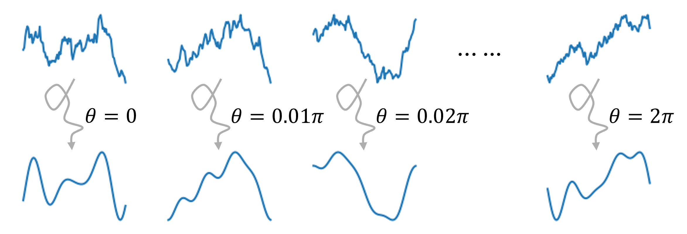
(b)

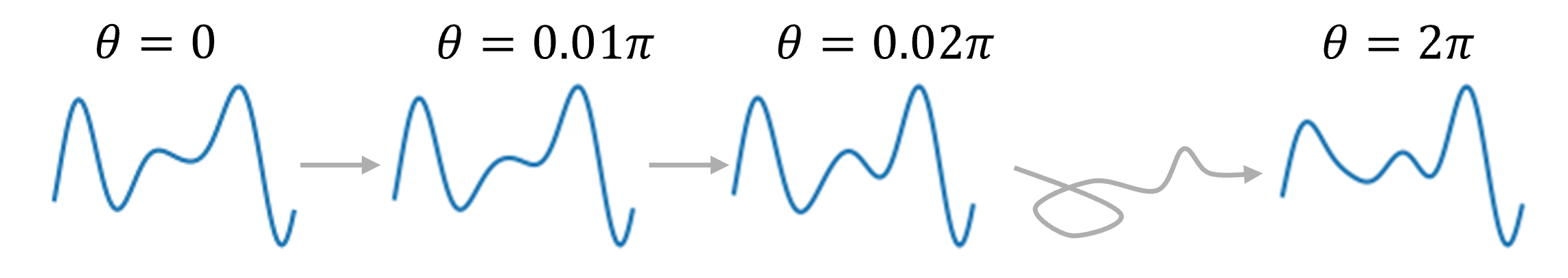
Figure 2: Comparison of different approaches to optimize robust control for parametric gates: (a) traditional way using optimization algorithms and (b) our way by traversing a level set using the RIPV algorithm.

In this chapter, we introduce the Robustness-Invariant Pulse Variance (RIPV) algorithm, which is designed to modify control pulses while maintaining robustness. The algorithm achieves this by ensuring that the control remains within the same level set of a robustness function. We assume the Hamiltonian governing the system is

$$H(t)=H_{\text{s}}+H_{\text{c}}(t)+H_{\text{n}}(t)\>,$$

the control Hamiltonian is

$$H_{\text{c}}=\sum_{k}\Omega_{k}(t;\mathbf{A})H_{\text{c},k}\>,$$

and the noise Hamiltonian is

$$H_{\text{n}}=\sum_{j}\delta_{j}H_{\text{n},j}\>.$$

Starting with a known robust control $H_{\text{c}|\theta=\theta_{0}}(t)$ for a parametric gate $U(\theta_{0})$, which is robust against $K$ noise sources $H_{\text{n},k}$ ($k=1,\dots,K$), the algorithm systematically varies the control Hamiltonian to identify a series of robust controls $H_{\text{c}|\theta}(t)$ for each parametric gate $U(\theta)$. Throughout this process, it ensures that the robustness functions $\mathcal{R}_{k}$ for each noise source $H_{\text{n},k}$ remains unchanged, thus preserving robustness. The RIPV algorithm is inspired by the unitary D-MORPH algorithm  [25], which explores a level set in a quantum control landscape, but they differ in both approach and application.

IV.1 RIPV for single control preview

Suppose we want to implement $U(\theta)$ robustly, where $\theta$ represents a gate parameter, typically the Bloch sphere’s rotation angle around some axis. We temporarily assume single control

$$H_{\text{c}}=\Omega(t;\mathbf{A})H_{\text{c},0}\>.$$

By assuming that $[H_{\text{s}},H_{\text{c},0}]=0$, we focus on the simplest case so that we will not generate rotation on other axes without influence of noise. We aim to find an $\mathbf{A}_{\theta}$ that implements the quantum gate $U(\theta)$ for each value of $\theta$ in $[\theta_{L},\theta_{R}]$ at intervals of $\Delta\theta$. Occasionally, we will refer to $\mathbf{A}$ as the “pulse” in this context when the meaning is clear. The procedure to implement $U(\theta)$ with equal robustness $\mathcal{R}$ to one noise source is as follows.

1. (Initialization.) Starting from an arbitrary pulse $\mathbf{A}_{\text{init}}$ (called the initial pulse), use any optimization algorithm to optimize the robustness function $\mathcal{R}(\mathbf{A})$. After optimization, we get a pulse $\mathbf{A}_{0}$ and its corresponding gate parameter $\theta_{0}$. Note that we only record but not designate the value $\theta_{0}$.

2. (Variation step.) Starting from $\mathbf{A}_{0}$ (called the beginning pulse), we add to it each time a small vector $\Delta\mathbf{A}$. But we choose $\Delta\mathbf{A}$ smartly so that $\mathcal{R}$ stays the same but $\theta$ changes by ${\Delta\theta}$. I.e., we require, in each step,

   $$\mathcal{R}(\mathbf{A}+\Delta\mathbf{A}) =\mathcal{R}(\mathbf{A})$$ (14)

   $$\theta(\mathbf{A}+\Delta\mathbf{A}) =\theta(\mathbf{A})\pm{\Delta\theta}\>.$$ (15)

   The sign before $\Delta\theta$ is determined by whether one wants to increase $\theta$ (when $\theta_{0}\leq\theta_{L}$) or decrease it (when $\theta_{0}\geq\theta_{R}$). After variation, we record the value of $\mathbf{A}_{1}=\mathbf{A}_{0}+\Delta\mathbf{A}$ and $\theta_{1}=\theta(\mathbf{A}_{1})$.

3. (Termination condition.) Repeat the variation step for $M$ iterations. We get controls $\mathbf{A}_{0},\allowbreak\mathbf{A}_{1},\dots\allowbreak,\allowbreak\mathbf{A}_{M}$ with $\theta_{0},\allowbreak\theta_{1},\dots,\theta_{M}$. Terminate when $[\theta_{0},\theta_{M}]$ covers the desired range $[\theta_{L},\theta_{R}]$. In the desired range, we get $N+1$ pulses where $N=\left\lceil\frac{\theta_{R}-\theta_{L}}{\Delta\theta}\right\rceil$. To aid discussions, it is sufficient to focus on the case where the variation of $\theta$ starts exactly at $\theta_{L}$ and ends at $\theta_{R}$, which is the assumption from now on.

4. (Relabel and output.) We relabel the $N$ pulses with $0,\allowbreak 1,\dots,\allowbreak N$. Finally, we get $N+1$ pulses $\mathbf{A}_{0},\allowbreak\mathbf{A}_{1},\dots,\allowbreak\mathbf{A}_{N}$, along with gate parameters $\theta_{L}=\theta_{0},\theta_{1},\dots,\theta_{N}=\theta_{R}$.

Here we implicitly assumed only one noise source, hence only one robustness function $\mathcal{R}$ to optimize and maintain. If there are multiple, we simply require Equation 14 for every robustness function $\mathcal{R}_{k}$ against $H_{\text{n},k}$ .

But a core question remains: How can we “smartly” choose $\Delta\mathbf{A}$ so that $\mathcal{R}$ does not change but $\theta$ increase or decrease by a proper amount that fits our need? We use Gradient Orthogonal Variation, which we introduce in the next section.

IV.2 Gradient Orthogonal Variation

Now we introduce the core of the RIPV algorithm, which is the Gradient Orthogonal Variation (GOV) algorithm. The goal of GOV is to modify the input vector $\mathbf{A}$ while keeping certain functions of $\mathbf{A}$ unchanged. These unchanged functions, referred to as “constraints,” are not limited to robustness and are denoted by a different font, $R_{1}(\mathbf{A}),\dots,R_{n}(\mathbf{A})$. It is important to note that these “constraints” differ from the traditional definition, as they are not required to satisfy specific bounds or inequalities but instead must remain invariant.

IV.2.1 Variation condition

Let’s transform Equation 14 into a more useful condition.

Recall that in calculus, we have this simple equation $\differential{y}=\derivative{y}{x}\differential{x}$ that states the infinitesimal change of $y$ as a function of $x$ is equal to the infinitesimal change of $x$ multiplied by the derivative $\derivative{y}{x}$. This holds true approximately when we numerically change $x$ by a small enough $\Delta x$.

Now in RIPV, we need to “smartly” choose $\Delta\mathbf{A}$ so that $\Delta R=R(\mathbf{A}+\Delta\mathbf{A})-R(\mathbf{A})=0$. Suppose we choose an infinitesimal $\differential{\mathbf{A}}$. In the tangent space, this amounts to choosing $\differential{\mathbf{A}}\neq 0$ so that $\differential{R}=0$. Hereinafter, we denote the change of $\mathbf{A}$ by $\differential{\mathbf{A}}$ to indicate the change is sufficiently small that it approximates the tangent space. For the robustness function $R(\mathbf{A})$, we have similarly

$$\differential{R}=\partialderivative{R}{\mathbf{A}}\cdot\differential{\mathbf{A}}\>.$$

In this equation, the derivative $\partialderivative{R}{\mathbf{A}}$ is taken with regard to a vector $\mathbf{A}$, which actually means taking the gradient $\nabla R$. We will stick to partial derivative notation to clearly indicate the variable with respect to which the gradient is taken. Since we want $\differential{\mathbf{A}}\neq 0$ and, in general, $\partialderivative{R}{\mathbf{A}}\neq 0$ holds, the only way to get $\differential{R}=0$ is to enforce the condition

$$\text{Variation condition:}\quad\differential{\mathbf{A}}\perp\partialderivative{R}{\mathbf{A}}\>.$$ (16)

The variation condition can be satisfied by simply selecting an arbitrary vector $\differential{\mathbf{A}}^{\text{pre}}$ as what we call “pre-variation”, and then performing the Gram-Schmidt process to get the component $\differential{\mathbf{A}}^{\text{pre}}_{\perp}$ that is perpendicular to $\partialderivative{R}{\mathbf{A}}$. This gives us the direction of $\differential{\mathbf{A}}$, after which we still have to adjust its length. In order to understand the significance of the pre-variation during GOV, we first take a look at orthogonalization.

IV.2.2 Orthogonalization

In short, the Gram-Schmidt process orthogonalizes a vector $\mathbf{v}$ to a group of vectors $\mathbf{u}_{1},\mathbf{u_{2},\dots,\mathbf{u}}_{N}$. The process is mathematically equivalent to decomposing $\mathbf{v}$ as

$$\mathbf{v}=\mathbf{v}_{\perp}+\mathbf{v}_{\parallel}\>,$$

where $\mathbf{v}_{\perp}$ (or $\mathbf{v}_{\parallel}$) is orthogonal to (or inside) $\mathrm{span}\{\mathbf{u}_{i}\}_{i}=\mathrm{span}\{\mathbf{u}_{1},\dots,\mathbf{u}_{N}\}$.

To get a $\differential{\mathbf{A}}$ that maintains a constraint $R$, we decompose an arbitrary pre-variation vector $\differential{\mathbf{A}}^{\text{pre}}$ as

$$\differential{\mathbf{A}}^{\text{pre}}=\differential{\mathbf{A}}^{\text{pre}}_{\perp}+\differential{\mathbf{A}}^{\text{pre}}_{\parallel}\>,$$

where $\differential{\mathbf{A}}^{\text{pre}}_{\perp}$ ($\differential{\mathbf{A}}^{\text{pre}}_{\parallel}$) is perpendicular (parallel) to the gradient $\partialderivative{R}{\mathbf{A}}$. We then vary $\mathbf{A}$ along the direction $\differential{\mathbf{A}}^{\text{pre}}_{\perp}$. By Equation 16, we know that $R$ is maintained.

If we want to keep $R_{1}(\mathbf{A}),\dots,R_{n}(\mathbf{A})$ constant, we still apply Gram-Schmidt process to get $\differential{\mathbf{A}}^{\text{pre}}_{\perp}$ (or $\differential{\mathbf{A}}^{\text{pre}}_{\parallel}$) that is orthogonal to (or inside) $\mathrm{span}\{\partialderivative{R_{i}}{\mathbf{A}}\}_{i}$. We then vary $\mathbf{A}$ along the direction $\differential{\mathbf{A}}^{\text{pre}}_{\perp}$. The tangent sub-bundle $\left(\mathrm{span}\{\partialderivative{R_{i}}{\mathbf{A}}\}_{i}\right)^{\perp}$, which is orthogonal to $\mathrm{span}\{\partialderivative{R_{i}}{\mathbf{A}}\}_{i}$, is the tangent subspace in which our variation happens. We refer to it by the variation subspace and denote it hereinafter by $V$.

IV.2.3 Choice of pre-variation

The selection of this pre-variation $\differential{\mathbf{A}}^{\text{pre}}$ is very important to roughly determine the direction along which the pulse $\mathbf{A}$ should be adjusted, since the “official variation” $\differential{\mathbf{A}}$ is an orthogonal projection of $\differential{\mathbf{A}}^{\text{pre}}$ into the variation subspace $V$. This choice can be tailored according to specific requirements.

The simplest choice would be a random vector. This would allow one to trace a stochastic trajectory in the space of control parameters, which lies in the level set of the QCRL. It is useful when exploring the level sets.

Another application is to maximize some objective function $F(\mathbf{A})$, for example, the fidelity of control. The fastest direction that maximizes $F(\mathbf{A})$ is $\partialderivative{F}{\mathbf{A}}$, because

$${\differential{F}}={\partialderivative{F}{\mathbf{A}}\cdot\differential{\mathbf{A}}}\leq\norm{\partialderivative{F}{\mathbf{A}}}\cdot\norm{\differential{\mathbf{A}}}\>.$$

The equality holds if and only if $\partialderivative{F}{\mathbf{A}}\parallel\differential{\mathbf{A}}$, or equivalently $\differential{\mathbf{A}}=\alpha\partialderivative{F}{\mathbf{A}}$ for some $\alpha>0$. Setting $\differential{\mathbf{A}}$ to $\alpha\partialderivative{F}{\mathbf{A}}$ with $\alpha<0$ (or $\alpha>0$) without GOV procedure gives the classic Gradient Descent (Ascent) algorithm. If we set $\differential{\mathbf{A}}^{\text{pre}}=\partialderivative{F}{\mathbf{A}}$ and $\differential{\mathbf{A}}=\alpha\differential{\mathbf{A}}^{\text{pre}}_{\perp}$, where $\differential{\mathbf{A}}^{\text{pre}}_{\perp}\in V$ and $\alpha>0$, then $\differential{\mathbf{A}}$ would generally not be the fastest direction to maximize $F(\mathbf{A})$. However, it is still the fastest direction to maximize $F(\mathbf{A})$ while keeping while keeping $\{R_{i}\}_{i}$ unchanged, for the following reasons. It maximizes $F(\mathbf{A})$, because the Gram-Schmidt process ensures the angle $\angle\left(\differential{\mathbf{A}}^{\text{pre}}_{\perp},\differential{\mathbf{A}}^{\text{pre}}\right)$ is an acute angle, i.e. it ensures $\differential{\mathbf{A}}^{\text{pre}}_{\perp}\cdot\partialderivative{F}{\mathbf{A}}\geq 0$. Therefore,

$$\differential{F}=\partialderivative{F}{\mathbf{A}}\cdot\differential{\mathbf{A}}=\partialderivative{F}{\mathbf{A}}\cdot\alpha\differential{\mathbf{A}}^{\text{pre}}_{\perp}>0\>.$$

It is also the fastest, because in the tangent subspace $\left(\mathrm{span}\{\partialderivative{R_{i}}{\mathbf{A}}\}_{i}\right)^{\perp}$ that keeps $\{R_{i}\}_{i}$ unchanged, the orthogonal projection $\differential{\mathbf{A}}^{\text{pre}}_{\perp}$ is the vector closest to $\differential{\mathbf{A}}^{\text{pre}}\!=\partialderivative{F}{\mathbf{A}}$, i.e., closest to the direction that $\theta$ increases. In summary, setting

$$\differential{\mathbf{A}}^{\text{pre}}=\partialderivative{F}{\mathbf{A}},\quad\differential{\mathbf{A}}=\alpha\differential{\mathbf{A}}^{\text{pre}}_{\perp}$$

where $\differential{\mathbf{A}}^{\text{pre}}_{\perp}\in\left(\mathrm{span}\{\partialderivative{R_{i}}{\mathbf{A}}\}_{i}\right)^{\perp}$ and with constant $\alpha>0$, one could maximize a function $F(\mathbf{A})$.

Lastly, we consider our RIPV algorithm, where the goal is to continuously traverse a function $\theta(\mathbf{A})$ within the interval $[\theta_{L},\theta_{R}]$. Starting at $\theta_{L}$, the variation process aims to conclude at $\theta_{R}$. To ensure $\theta$ is increasing, we define the pre-variation as $\differential{\mathbf{A}}^{\text{pre}}=\partialderivative{\theta}{\mathbf{A}}$. However, the magnitude of $\differential{\mathbf{A}}$ must be more carefully chosen to ensure that $\theta$ evolves smoothly, with evenly spaced increments throughout the process.

IV.2.4 Normalization

Now that the direction of variation is determined as $\differential{\mathbf{A}}^{\text{pre}}_{\perp}$, another important question concerns the step size of variation. Since our goal is to implement $U(\theta)$ for all values of $\theta$, we want $\theta$ to be evenly distributed across the interval $[\theta_{L},\theta_{R}]$, with an ideal step size of ${\Delta\theta}_{\text{ideal}}$. The linear part of variation $\differential{\theta}$, caused by $\differential{\mathbf{A}}$, is determined by the differential relation ${\differential{\theta}}={{\partialderivative{\theta}{\mathbf{A}}}\cdot\differential{\mathbf{A}}}$. Then we would want ${\differential{\theta}}={\Delta\theta}_{\text{ideal}}$, i.e.

$$\norm{\differential{\mathbf{A}}} =\frac{{\Delta\theta}_{\text{ideal}}}{\norm{\partialderivative{\theta}{\mathbf{A}}}\cdot\cos\angle\left(\differential{\mathbf{A}}^{\text{pre}}_{\perp},\partialderivative{\theta}{\mathbf{A}}\right)}$$

$$=\frac{{\Delta\theta}_{\text{ideal}}}{\norm{\partialderivative{\theta}{\mathbf{A}}}}\cdot\frac{\norm{\differential{\mathbf{A}}^{\text{pre}}_{\perp}}\cdot\norm{\partialderivative{\theta}{\mathbf{A}}}}{\langle\differential{\mathbf{A}}^{\text{pre}}_{\perp},\partialderivative{\theta}{\mathbf{A}}\rangle}$$

$$=\frac{{\Delta\theta}_{\text{ideal}}\cdot\norm{\differential{\mathbf{A}}^{\text{pre}}_{\perp}}}{\langle\differential{\mathbf{A}}^{\text{pre}}_{\perp},\partialderivative{\theta}{\mathbf{A}}\rangle}\>,$$

where $\angle(\mathbf{u},\mathbf{v})$ denotes the angle between two vectors $\mathbf{u}$ and $\mathbf{v}$. Then the “official variation” should be the unit vector $\differential{\mathbf{A}}^{\text{pre}}_{\perp}/\norm{\differential{\mathbf{A}}^{\text{pre}}_{\perp}}$ multiplied by this magnitude, which is

$$\differential{\mathbf{A}}=\frac{{\Delta\theta}_{\text{ideal}}}{\langle\differential{\mathbf{A}}^{\text{pre}}_{\perp},\partialderivative{\theta}{\mathbf{A}}\rangle}\differential{\mathbf{A}}^{\text{pre}}_{\perp}\>.$$

IV.2.5 Summary of GOV

To summarize, the goal of GOV is to maintain constraints $\{R_{i}\}_{i}$ unchanged, for which we need to achieve the variation condition $\differential{\mathbf{A}}\perp\partialderivative{R_{i}}{\mathbf{A}}$. The general procedure is as follows.

1. Choose an arbitrary pre-variation vector $\differential{\mathbf{A}}^{\text{pre}}$, either random or tasked-specific.

2. Apply the Gram-Schmidt process to get $\differential{\mathbf{A}}^{\text{pre}}_{\perp}\in\left(\mathrm{span}\{\partialderivative{R_{i}}{\mathbf{A}}\}_{i}\right)^{\perp}$.

3. Choose an appropriate $\alpha$ according to the task, and vary $\mathbf{A}$ by $\differential{\mathbf{A}}=\alpha\differential{\mathbf{A}}^{\text{pre}}_{\perp}$.

For our RIPV algorithm, where we traverse the rotation angle $\theta$ while maintaining several fixed criteria $\{R_{i}\}_{i}$, we need to further specify the pre-variation $\differential{\mathbf{A}}^{\text{pre}}$ and normalization factor $\alpha$.

1. Calculate the pre-variation $\differential{\mathbf{A}}^{\text{pre}}=\partialderivative{F}{\mathbf{A}}$.

2. Apply the Gram-Schmidt process to get $\differential{\mathbf{A}}^{\text{pre}}_{\perp}\in\left(\mathrm{span}\{\partialderivative{R_{i}}{\mathbf{A}}\}_{i}\right)^{\perp}$.

3. Normalize the vector and adjust the step size to get $\differential{\mathbf{A}}=\frac{{\Delta\theta}_{\text{ideal}}}{\langle\differential{\mathbf{A}}^{\text{pre}}_{\perp},\partialderivative{\theta}{\mathbf{A}}\rangle}\differential{\mathbf{A}}^{\text{pre}}_{\perp}$.

The GOV algorithm extends beyond robust quantum optimal control aimed at countering quasi-static noise. It allows for adjusting the rotation angle while preserving robustness against any form of noise or leakage, or conversely, enhancing robustness without compromising the fidelity to a specific gate. Moreover, its applicability is not limited to quantum control tasks. Whenever parameter variation is needed without altering certain criteria, the GOV algorithm proves to be a valuable tool.

IV.2.6 Variation vs. optimization

Traversing a level set, such as when implementing a robust parametric gate, is fundamentally different from an optimization algorithm (referred to as “OPT” in this section) and cannot naturally be formulated as one. The goal is not to optimize anything, but rather to vary the solution. Therefore, we refer to this type of algorithm as a variation algorithm (referred to as “VAR” in this section).

There are at least three key differences between variation and optimization algorithms.

Goal.

OPT aims to find the optimal solution, whereas VAR seeks a set of solutions that share the same constraint values (e.g., robustness) as the beginning solution, regardless of optimality.

Role of constraints.

The term “constraint” has a slightly different meaning. In VAR, constraints must remain unchanged, serving as the goal of the algorithm. In OPT, constraints must be equal to or less than some predefined values, serving as obstructions to our goal – optimization.

Role of intermediate solutions.

In OPT, we solve equations or inequalities only once to find the optimal solution, such as with Lagrange multipliers. Even in gradient descent, we only need the final result. In contrast, VAR collects all the intermediate solutions, requiring the variation condition to be solved multiple times. It is more comparable to solving differential equations, where each intermediate step provides one slice of the final solution function.

IV.3 RIPV algorithm implementation

Knowing how to choose the variation $\differential{\mathbf{A}}$ so that $\mathcal{R}$ (or multiple $R_{i}$’s) will not change, we can complete the RIPV algorithm. We firsts discuss some details, and then present the algorithm’s pseudocode.

IV.3.1 Extraction of rotation angle

For the simplest control scheme $H_{\text{c}}(t)=\Omega(t)\sigma$ where $\sigma$ is a constant operator, the rotation angle is simply the integral $\theta(\mathbf{A})=\int_{0}^{T}\Omega(t;\mathbf{A})\differential{t}$. For example, if we want to implement $R_{x}(\theta)$ with $\sigma_{x}$ control, then this integration gives the exact rotation angle $\theta$ without the risk of extra rotation along undesired axes, because the control scheme allows only $\sigma_{x}$ rotation.

However, if the control involves more than one term, the rotation angle can no longer be calculated by simple integration. An even worse problem is that two non-commuting time-dependent operators can generate rotations along a third axis. For example, the control scheme $H_{\text{c}}(t)=\Omega_{x}(t)\sigma_{x}+\Omega_{y}(t)\sigma_{y}$ can even implement an $R_{z}(\theta)$ gate.

To extract the rotation angle from the noiseless propagator $U_{\text{sc}}(T)=U^{H_{\text{s}}+H_{\text{c}}(\tau)}(T)$, we can compute the matrix logarithm to get its exponent $\eta$ and then project $\eta$ onto the desired rotation axis $\sigma$. The $\sigma$ here is a Pauli matrix in single-qubit control. For a $d$ dimensional Hilbert space, the matrix inner product $\tr(\eta^{\dagger}\sigma)/d$ gives the coefficient of $\eta$ along $\sigma$, which, multiplied by $d$, gives the rotation angle by the axis $\sigma$. Additionally, we must ensure that the rotation angles $\vartheta_{j}$ along all undesired axes $\varsigma_{j}$ remain zero ($\vartheta,\varsigma$ are variant forms of $\theta,\sigma$, here denoting undesired angles/axes).

In summary, the rotation angle along an axis $\sigma$ can be determined as

$$\theta =\Tr\left(\eta^{\dagger}\sigma\right)/d, \text{where}\quad\eta =i\operatorname{logm}U_{\text{sc}}(T)\>,$$

where $\operatorname{logm}$ stands for matrix logarithm. Meanwhile, in addition to preserving robustness throughout the variation process, we must also ensure the rotation angles $\vartheta_{j}=\tr(\eta^{\dagger}\varsigma_{j})$ along undesired axes $\varsigma_{j}$, remains at zero.

IV.3.2 Calculation of derivatives

We need to calculate the value of the derivatives $\partialderivative{\theta}{\mathbf{A}}$ and $\partialderivative{R_{i}}{\mathbf{A}}$ at data points. These could be carried out and hard-coded into the program, but we adopted a more general solution, Automatic Differentiation, hereinafter referred to as autodiff.

Autodiff, short for automatic differentiation, is fundamentally different from numerical differentiation and offers significant advantages in computational complexity. It is a technique implemented in libraries such as TensorFlow, PyTorch, and Jax, which automatically compute derivatives alongside function evaluations. Unlike numerical differentiation, which approximates derivatives by introducing small perturbations, autodiff constructs a computation graph that tracks the data flow during function evaluation. This graph enables the differentiator to retrieve exact derivative formulas and efficiently apply the chain rule to compute derivatives directly with respect to every free variable. While numerical methods require $n$ passes to calculate derivatives for $n$ variables, autodiff achieves this in a single pass with a bit of overhead.

To calculate the derivatives that we need, one only has to change the ordinary numbers and vectors into the traceable (or differentiable) variables provided by the autodiff library so that it can automatically construct the computation graph and output derivatives.

IV.3.3 Single noise source

Data: Initial pulse with $\mathbf{A}_{0}$ that implements $\theta_{0}=\theta_{L}$, rotation angle range $[\theta_{L},\theta_{R}]$, variance step size ${\Delta\theta}_{\text{ideal}}$

Result: An array of pairs of rotation angle and pulse parameters records $=\{(\theta_{k},\mathbf{A}_{k})\}_{k}$

1 Initialize the pulse parameter iterator $\mathbf{A}^{\text{now}}\leftarrow\mathbf{A}_{0}$ ;

2 Initialize the rotation angle $\theta\leftarrow\theta_{0}$ ;

3 Record the first pair records.append($\theta_{0},\mathbf{A}_{0}$) ;

4 while  $\theta^{\textup{now}}<\theta_{R}$  do

5    Calculate $\theta^{\text{now}}$ and $\mathcal{R}^{\text{now}}$ from $\mathbf{A}^{\text{now}}$ with autodiff on ;

6    Calculate $\displaystyle\differential{\mathbf{A}}^{\text{pre}}\leftarrow\evaluated{\partialderivative{\theta}{\mathbf{A}}}_{\mathbf{A}^{\text{now}}}$ using autodiff ;

7    Calculate $\displaystyle\evaluated{\partialderivative{\mathcal{R}}{\mathbf{A}}}_{\mathbf{A}^{\text{now}}}$ using autodiff ;

8    Perform Gram-Schmidt process $\displaystyle\differential{\mathbf{A}}^{\text{pre}}=\differential{\mathbf{A}}^{\text{pre}}_{\perp}+\differential{\mathbf{A}}^{\text{pre}}_{\parallel}$ so that $\displaystyle\differential{\mathbf{A}}^{\text{pre}}_{\perp}\perp\partialderivative{\mathcal{R}}{\mathbf{A}}$ ;

9    Normalize $\differential{\mathbf{A}}^{\text{pre}}_{\perp}$ according to ${\Delta\theta}_{\text{ideal}}$, $\displaystyle\differential{\mathbf{A}}\leftarrow\frac{{\Delta\theta}_{\text{ideal}}}{\left\langle\partialderivative{\theta}{\mathbf{A}},\differential{\mathbf{A}}^{\text{pre}}_{\perp}\right\rangle}\cdot\differential{\mathbf{A}}^{\text{pre}}_{\perp}$ ;

10    Vary the current value of $\mathbf{A}$, $\mathbf{A}^{\text{now}}\leftarrow\mathbf{A}^{\text{now}}+\differential{\mathbf{A}}$ ;

11    Record a new pair records.append($\theta^{\textup{now}},\mathbf{A}^{\textup{now}}$) ;

12   

13 end while

Algorithm 1 RIPV for single control single noise

The simplest RIPV algorithm can deal with one control term $H_{\text{c},0}$ and one quasi-static noise source $H_{\text{n},0}$, where the commutator $[H_{\text{c},0},H_{\text{n},0}]\neq 0$. We only have to vary one rotation angle $\theta$ and maintain one robustness $\mathcal{R}$. The pseudocode of single control single noise scenario is shown in algorithm 1. If we use the $n$-th order asymptotic robustness as constraint in RIPV, we refer to this algorithm as $n$-th order RIPV.

IV.3.4 Multiple noise sources

To deal with multiple noise sources, especially quasi-static noise on the control term, we need to upgrade our control and modify two steps of the RIPV algorithm. But before the general scenario, let’s look at a simpler case.

If we assume $H_{\text{c}}(t)=\Omega(t)H_{\text{c},0}$ satisfying $[H_{\text{s}},H_{\text{c}}]=0$ as in subsection IV.1, this simplest control model will never generate any extra rotation on undesired axes. Hence, only noise could undermine the goal of our control task. In this case, if we try to fight against multiple error sources that are all orthogonal to the control term $H_{\text{c},0}$, we simply need to add the robustness function for every noise source into our constraints. This single control, multiple noise sources scenario is fundamentally the same as the single noise source case.

On the other hand, if $[H_{\text{s}},H_{\text{c}}]\neq 0$ or there are more than one control term, we need to consider undesired rotations. If we apply arbitrary pulses $\{\Omega_{k}(t)\}_{k}$ to $\{H_{\text{c},k}\}_{k}$, it is not guaranteed to produce rotation $\theta$ on the axis that we want. That means we need to modify two steps in the RIPV algorithm for single noise source. Suppose we want to generate rotation on $\sigma$ by $\theta$, while the rotation on $\varsigma_{j}$, or $\vartheta_{j}$ should be $0$. Modification 1. Since the rotation angle is no longer a simple integration of the pulse, we have to use the projection method mentioned in subsubsection IV.3.1 instead of simple integration to calculate rotation angles, whether it is $\theta$ or $\vartheta_{j}$. Modification 2. In the orthogonalization step, we should orthogonalize $\differential{\mathbf{A}}^{\text{pre}}$not only to the gradients of robustness functions, but also the undesired rotation angles.

For example, let’s say we want to implement $R_{x}(\theta)$ that are robust to noise on $\sigma_{x}$, $\sigma_{y}$ and $\sigma_{z}$. Then we have five constraints, namely $\mathcal{R}_{x},\mathcal{R}_{y},\mathcal{R}_{z},\vartheta_{y}$ and $\vartheta_{z}$. We need to maintain $\mathcal{R}_{x}$, $\mathcal{R}_{y}$ and $\mathcal{R}_{z}$ so that the robustness on the three operators are unchanged throughout the variation, and we also need to maintain $\vartheta_{y}$ and $\vartheta_{z}$ so that they remain zero throughout the variation.

This modification is very important because it is often the case that we have multiple controls when fighting off multiple noise sources. The prerequisite for dynamical noise-cancellation is having an “orthogonal control”. Concretely, from the previous work [40], we have known that, in order to correct error in direction $\sigma$, we need to have a control in an orthogonal direction of $\sigma$. In other words, for each noise source $H_{\text{n},k}$, there should be at least one control term $H_{\text{c},j}$ satisfying $[H_{\text{n},k},H_{\text{c},j}]\neq 0$. One special case is that we want to cancel the quasi-static noise on the control term, then the control cannot correct the noise on itself. Then we would need at least two controls to cancel the noise on each other.

IV.4 Numerical considerations

In this section, we discuss some technical problems when implementing the RIPV algorithm numerically.

IV.4.1 Number of parameters

The number of independent control parameters, equivalently the dimension of the landscape, matters. It must be sufficiently large to accommodate a viable solution and ensure that the solution can be easily accessed within a given level set (which is called reachability). This is intuitively easy to understand: after all, more parameters means more choices. Now let’s sort out the details.

First, let’s consider at exactly which step do we need a large enough dimension and how large it must be. Remember that after we chose a pre-variation $\differential{\mathbf{A}}^{\text{pre}}$, we then have to orthogonalize it to the set of constraints $\{R_{i}\}_{i}$. Generally, if we have $m$ constraints $\{R_{1},\dots,R_{m}\}$, their gradients would span an $m$-dimensional space $V^{m}=\mathrm{span}\{\partialderivative{R_{i}}{\mathbf{A}}\}_{i=1}^{m}$. Now we want the “official” $\differential{\mathbf{A}}$ to be orthogonal to $V^{m}$, then we must live in a space at least $(m+1)$-dimensional. However, if it is exactly $(m+1)$-dimensional, then we would have no choice but to follow the only direction that is orthogonal to $V^{m}$. That would invalidate our choice of $\differential{\mathbf{A}}^{\text{pre}}$ because we actually have no freedom in choosing direction. In summary, we need at least $m+2$ independent parameters if we want to maintain $m$ constraints.

Second, having more parameters is still beneficial. In essence, we are looking for a direction that is orthogonal to $V^{m}$, so it is the best if the “probability of being orthogonal” is higher. If we consider strict orthogonality, then, in a $n$-dimensional parameter space, the probability of two vectors being orthogonal is simply $\frac{n-1}{n}$. However, since we are running a numerical algorithm, where everything has a numerical precision limit, we actually only test approximate orthogonality where the angle between two vectors is $\frac{\pi}{2}\pm\epsilon$ for very small $\epsilon$. A corollary from the Johnson–Lindenstrauss lemma states that for a fixed $\epsilon$, the probability of $\frac{\pi}{2}\pm\epsilon$ orthogonal grows exponentially with the dimension $n$. In Figure 3, we show a simple simulation where we take 5000 random vectors and ask for the distribution of the angle between each pair of vectors. Even rasing dimension from 7 to 10 results in a visible rise of probability. If we have 100 parameters (though unlikely), we can see that “almost all” pairs of vectors have have an angle between them in $[80,100]$ degrees. In summary, we would have a better chance at locating a direction orthogonal to $V^{m}$ if our parameter space has higher dimension.

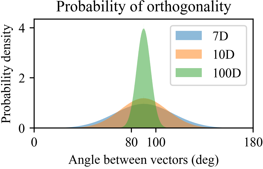
Figure 3: Probability of two vectors being orthogonal in an $n$-dimensional parameter space. This is a histogram of $10^{5}$ randomly generated vectors.

IV.4.2 Error from linear approximation

The RIPV algorithm inevitably introduces error when it takes finite-length steps in the tangent space of the level set instead of the actual level set. Now matter how small a step we choose for variation, we can only slow down the accumulation of error but not eliminate it. This problem can be dealt with by an extra correcting step between two consecutive variation steps where we bring our solution back to the level set. In the unitary D-MORPH algorithm that inspired our RIPV, they applied correcting methods through unitary tracking and brought the algorithm’s precision to machine precision.

In our algorithm, since we used autodiff, we can insert a gradient-based optimization procedure after taking the variation step in order to keep the parameters on the level set. Suppose we are at a point on the level set of $\mathcal{R}=\mathcal{R}_{0}$ with $\theta=\theta_{k}$, and a variation in the parameters moves $\theta$ to $\theta_{k+1}$, resulting in a deviation to a neighboring level set $\mathcal{R}=\mathcal{R}_{0}+\epsilon$. One way is to apply the simplest gradient descent to optimize the sum of the fidelity to $U(\theta_{k+1})$ and the robustness deviation $\mathcal{R}-\mathcal{R}_{0}$. A more complex way is to ensure we only deviate to a more robust level set. If $\epsilon<0$, we can apply a mini GOV procedure, with the only difference being that we maintain the fidelity to $U(\theta_{k+1})$ while enhancing robustness, not the other way around like in RIPV.

In our numerical examples, these steps are not implemented because linear approximation is good for now. Also, this extra correcting step takes a lot of both coding effort and execution time.

IV.4.3 Viability of variation direction

Even if we used a lot of free parameters, there is still a chance that we cannot find a viable direction for $\differential{\mathbf{A}}$. This problem might appear when we orthogonalize $\differential{\mathbf{A}}^{\text{pre}}$ to $V^{m}=\mathrm{span}\{\partialderivative{R_{i}}{\mathbf{A}}\}_{i=1}^{m}$. If we chose the pre-variation $\differential{\mathbf{A}}^{\text{pre}}=\partialderivative{\theta}{\mathbf{A}}$ and found that $\partialderivative{\theta}{\mathbf{A}}\in V^{m}$, orthogonalization is impossible, which means we would not be able to increase or decrease $\theta$ without changing at least one $R_{i}$.

Let’s discuss what does this mean and how to avoid it. Let’s say we are currently at a point $\mathbf{A}_{0}$ in $\mathbb{R}^{n}$, the space of $n$ real parameters $\{A_{i}\}_{i=1}^{n}$. Normally we can expect

$$\dim\left(\mathrm{span}\left\{\partialderivative{\theta}{\mathbf{A}},\partialderivative{R_{1}}{\mathbf{A}},\dots,\partialderivative{R_{m}}{\mathbf{A}},\right\}\right)=m+1\>,$$

which means $\partialderivative{\theta}{\mathbf{A}}$ cannot be spanned by $\partialderivative{R_{i}}{\mathbf{A}}$’s. We call $\mathbf{A}_{0}$ an irregular point if we find out $\partialderivative{\theta}{\mathbf{A}}\in V^{m}$, i.e. if $\partialderivative{\theta}{\mathbf{A}}$ has no component orthogonal to $\{\partialderivative{R_{i}}{\mathbf{A}}\}_{i=1}^{m}$.

An irregular point appears in one of the following cases.

1. The objective $\theta(\mathbf{A})$ is irregular at every point. In this case, no matter which value of $\mathbf{A}$ we try, $\partialderivative{\theta}{\mathbf{A}}$ is always a linear combination of $\partialderivative{R_{i}}{\mathbf{A}}$’s, as

   $$\partialderivative{\theta}{\mathbf{A}} =f_{1}(\mathbf{A})\partialderivative{R_{1}}{\mathbf{A}}+\dots+f_{m}(\mathbf{A})\partialderivative{R_{m}}{\mathbf{A}}\>.$$

   It means they are fundamentally dependent to each other and cannot be decoupled as objective and constraints. For instance, $\theta$ might be a function of $R_{i}$’s with $\partialderivative{\theta}{R_{i}}$ serving as $f_{i}$ (but this is stronger than the derivatives being linearly dependent):

   $$\partialderivative{\theta}{\mathbf{A}} =\partialderivative{\theta}{R_{1}}\partialderivative{R_{1}}{\mathbf{A}}+\dots+\partialderivative{\theta}{R_{m}}\partialderivative{R_{m}}{\mathbf{A}}\>.$$

   In this case, we have to change the objective function or constraints and check our physical model.

2. The objective $\theta(\mathbf{A})$ is irregular at a subset containing $\mathbf{A}_{0}$. In this case, we are just at an unlucky point $\mathbf{A}_{0}$. We can pull the current parameter point $\mathbf{A}_{0}$ to another parameter point $\mathbf{A}_{1}$ in a different, maybe more robust level set, using the same method as in the correcting step. Or, we can start off from a different parameter point in the hope of getting rid of this irregular point.

In our numerical experiments, non of the above happens. We presume the reason is the large number of parameters (18 when using both X and Y control for one qubit) makes the variation subspace large enough to accommodate a viable variation direction $\differential{\mathbf{A}}$.

IV.4.4 Interpolation of gate parameters

After all, we can only generate a discrete series of pulses, instead of a genuinely continuous series. It is not exactly what we need in reality where we must implement $U(\theta)$ for continuous values of $\theta$. However, since our algorithm is a local gradient-based algorithm, which means it traces a continuous path in the parameter space, the pulses $\Omega_{\theta_{1}}(t)$ and $\Omega_{\theta_{2}}(t)$ for $\theta_{1}$ and $\theta_{2}$ that are close to each other are also close as functions of $t$. This means we can interpolate between two pulses $\Omega_{\theta_{k}}(t)$ and $\Omega_{\theta_{k+1}}(t)$ to get a pulse $\Omega_{\theta}(t)$ with any intermediate $\theta\in[\theta_{k},\theta_{k+1}]$. More precisely, if we denote by $\mathbf{A}_{i}$ that implements $U(\theta_{i})$, we can interpolate on the $N$ solutions $\{(\theta_{i},\mathbf{A}_{i})\}_{i=1,\dots,N,}$ obtained by RIPV to get a continuous function $\mathbf{A}(\theta)$. This way, we can say we got a map from rotation angles to control pulses $\theta\mapsto\Omega_{\theta}=\Omega(t;\mathbf{A}(\theta))$.

This is another advantage of our RIPV algorithm over traditional algorithms that optimize each $U(\theta)$ separately: that we can effectively get a continuous function $\mathbf{A}(\theta)$. It is meaningful for experimentalists, because when numerical simulations and physical experiments disagree, we can calibrate $\theta$ by adjusting $\mathbf{A}$ values while keeping its robustness.

IV.5 Comparison to unitary D-MORPH

We mentioned earlier in section IV that our RIPV algorithm is inspired by the unitary D-MORPH algorithm by J. Dominy and H. Rabitz [25] with some important modifications.

Elementary description.

We specifically avoided the descriptive language of differential manifolds. Because, despite being extremely accurate and enlightening, it requires a lot of prior knowledge on the subject of manifolds, which is not necessarily familiar to quantum computing scientists and engineers. Instead, we adopted the language used in gradient descent.

Improved computational efficiency.

This algorithm uses less computational resources and computation time, because the unitary D-MORPH algorithm solves the whole needs to calculate the inverse of the overlap matrix $\mathcal{S}_{\mathcal{E},T}$ (notation borrowed from the original paper). The $\mathcal{S}_{\mathcal{E},T}$ means, roughly speaking, the linear map $\differential{\mathbf{A}}\to\differential{R}$ in the tangent space of some landscape $R(\mathbf{A})$, where $R$ is a landscape whose level sets correspond to realizing a fixed gate at a fixed time. But this computation is unnecessary because inverting $\mathcal{S}_{\mathcal{E},T}$ is effectively calculating all the possible directions that would keep us in the level set (i.e. keep $R$ unchanged), while we need only one direction. In contrast, our RIPV algorithm first assumes a “pre-variation” $\differential{\mathbf{A}}^{\text{pre}}$ and then calculates only the projection of $\differential{\mathbf{A}}^{\text{pre}}$ on to (the tangent space of) the level set. In this way, we avoids inverting a matrix by using Gram-Schmidt orthogonalization. This advantage is only visible when the dimension of Hilbert space $\mathcal{H}$ is large, because the number of columns (or rows) of $\mathcal{S}_{\mathcal{E},T}$ is the dimension of Hermitian operators on $\mathcal{H}$.

Versatility.

The RIPV, or more generally the GOV algorithm, is not limited to maintaining robustness. It makes no assumption on the structure or the number of the constraint functions. Calculations of the unitary D-MORPH was based on the goal to keep either the gate or the gate time fixed while changing the pulse. It cannot keep both fixed. But GOV can keep any number of constraints unchanged, regardless of the type of constraints, while improving one merit of the control or just randomly exploring the parameter space.

V Numerical examples

To demonstrate that we can actually generate an almost continuous series of control pulses to implement a quantum gate with a continuous parameter, we conducted several numerical experiments. Before we look into them, a little digression is needed to talk about a tool used in visualization.

V.1 Quantum Error Evolution Diagram

We cannot understand anything about the pulse if we just stared at the pulses that we generate, so we need some tool to visualize its properties, especially about how they respond to noise. When displaying our numerical results, we use a diagram called Quantum Error Evolution Diagram [41, 40], or QEED, to manifest the error induced by some noise source during the quantum gate operation. To put it simply, when we consider a 2-level quantum system, the error caused by a single noise source $\sigma$ through some time can be mapped to a 3D curve $\mathbf{r}_{\sigma}(t)$ parametrized by time $t$. If there are three noise sources in this 2-level system, namely $\sigma_{x}$, $\sigma_{y}$ and $\sigma_{z}$, we would get three 3D curves, which we call error curves, $\mathbf{r}_{\sigma_{x}}$, $\mathbf{r}_{\sigma_{y}}$ and $\mathbf{r}_{\sigma_{z}}$.

The curves $\mathbf{r}_{j}(t)$ (where $j=\sigma_{x},\sigma_{y},\sigma_{z}$) are closely related to the error evolution $U_{\text{n}}^{\text{sc}}(t)$ associated with noise in directions defined by $H_{\text{n}}=\sigma_{x},\sigma_{y},\sigma_{z}$. Since QEED is associated with $U_{\text{n}}^{\text{sc}}(t)$, which encodes information about the applied control, the QEED and the control can be mutually reconstructed from one another. Additionally, we can extract asymptotic robustness, as defined by the Magnus expansion, directly from the QEED. Concretely, if the control corrects quasi-static noise in a direction $\sigma$ to first order, meaning $\mathcal{R}^{1}_{\text{(M)}}=0$, then the curve $\mathbf{r}_{\sigma}$ should form a closed loop. Furthermore, second-order robustness to $\sigma$ noise implies that the curve $\mathbf{r}_{\sigma}$ will project onto the three coordinate planes in 3D with a net zero area in each projection.

When considering a single noise source and a single control, such as $H_{\text{n}}=\delta\sigma_{z}$ and $H_{\text{c}}=\frac{\Omega(t)}{2}\sigma_{x}$, the resulting error curve $\mathbf{r}_{\sigma_{z}}$ is confined to a 2D subspace. This subspace, spanned by $\sigma_{z}$ and $\sigma_{y}$, lies perpendicular to the control direction. The rotation angle $\theta=\int_{0}^{T}\Omega(t)\,dt$ can be inferred directly from the error curve as it is the angle between the initial and final directions of the curve’s tangent vector. Furthermore, if the curve $\mathbf{r}_{\sigma_{z}}$ forms a closed loop, this indicates that the control is first-order robust to $\sigma_{z}$ noise. A zero net area enclosed by the curve – such as in an “8”-shaped trajectory – implies second-order robustness. Hence, in the single control, single noise scenario, we will leverage the QEED, in combination with the control pulse, to directly demonstrate the robustness of the control to the readers.

V.2 Single qubit gates

In the rotation picture $e^{-it\omega_{d}\sigma_{z}}$ at the drive frequency, the most commonly used single qubit dynamic model is $H(t)=\frac{\Delta}{2}\sigma_{z}+\frac{\Omega_{x}(t)}{2}\sigma_{x}+\frac{\Omega_{y}(t)}{2}\sigma_{y}$, where $\Delta=\omega_{d}-\omega_{q}$ is the detuning between drive frequency $\omega_{d}$ and qubit frequency $\omega_{q}$. We operate in a on-resonance system, where $\Delta=0$ is assumed, i.e. the generally assumed form of our qubit model is $H(t)=\frac{\Omega_{x}(t)}{2}\sigma_{x}+\frac{\Omega_{y}(t)}{2}\sigma_{y}$.

V.2.1 Single noise source

In this part, we assume the noise is on $\sigma_{z}$. According to ref. [40], we need only control on either one of the perpendicular axes, which means control on either $\sigma_{x}$ or $\sigma_{y}$. We choose $\sigma_{x}$ as our control term to implement robust $R_{x}(\theta)$. To summarize, we assume

$$H_{\text{c}}(t) =\frac{\Omega(t)}{2}\sigma_{x}$$

$$H_{\text{n}} =\delta\sigma_{z}\>,$$

where $\delta$ is constant during the gate operation. The pulse $\Omega(t)$ is parameterized by an $(2n+1)$-dimensional vector $\mathbf{A}=(a_{0},\allowbreak a_{1},\allowbreak\dots,\allowbreak a_{n},\allowbreak\phi_{1},\allowbreak\dots,\allowbreak\phi_{n})$ as

$$\Omega(t;\mathbf{A})=\sin(\pi\tilde{t})\left(a_{0}+\sum_{k=1}^{n}a_{k}\cos(2\pi k\tilde{t}+\phi_{k})\right)\>,$$ (17)

where $\tilde{t}=t/T$ is time normalized by gate time $T=50\,\mathrm{ns}$. The beginning pulse parameters used in these simulations are all from ref. [40]. We will denote the pulse that implements $R_{x}(\theta)$ as $\Omega_{\theta}(t)$, its parametrization as $\Omega_{\theta}(t;\mathbf{A}_{\theta})$.

1st order robust $R_{x}(\theta)$.

In the first demonstration, we used 1st order RIPV, where $\mathcal{S}^{1}$ defined in Equation 10 is the only constraint. We started from a 2nd order robust pulse $\Omega_{2\pi}(t)$ implementing $R_{x}(2\pi)$, parameterized by Equation 17 with the values of $\mathbf{A}_{2\pi}$ given by $R_{\text{ex;}\perp}^{2\pi}$ in the supplementary materials of Hai’s paper [40]. We then varied the pulse $\Omega_{2\pi}(t)$ with pre-variation

$$\differential{\mathbf{A}^{\text{pre}}}=\partialderivative{\theta}{\mathbf{A}}\>,$$

to increase the rotation angle $\theta$ until it reaches $4\pi$. The step size was set to be

$${\Delta\theta}_{\text{ideal}}=0.001\,\mathrm{rad}\>,$$

which means we needed approximately $2\pi/0.001\approx 6283$ iterations. With these settings, we got a series of pulses $\Omega_{\theta}(t)=\Omega(t;\mathbf{A}_{\theta})$ with $\theta$ almost evenly distributed in $[0,2\pi]$ with an interval $0.001\,\mathrm{rad}$. Neglecting a global phase of $2\pi$, we can say we obtained control pulses that implements $R_{x}(\theta)$ for $\theta\in[0,2\pi]$. In our following discussions, this global phase will always be neglected and the beginning pulse is denoted as $\Omega_{0}(t)$.

In Figure 5(a-c), we showed respectively the pulses obtained by RIPV algorithm, the corresponding QEEDs, and the infidelity-noise graph, all colored by the value of $\theta$ from $0$ to $2\pi$. In the QEED (a) and pulse (b) figures, since we could not print an animation, we plotted the pulse series in a 3D graph for about 1 out of every 100 pulses, among which we highlight those with $\theta=\frac{n\pi}{3}$ for $n=0,1,2,3,4,5,6$. The infidelity-noise graph (c), on the other hand, are made half transparent and stacked in a 2D graph for better comparison. The noise strength are shown relative to the maximum amplitude of the pulse $\Omega_{m}=\max_{t\in[0,50]}\Omega(t)$. We also plot the infidelity for a non-robust pulse $\Omega(t)=\sin\pi\tilde{t}$ with dashed black line.

(a)

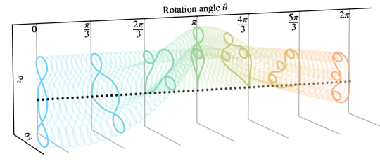
(b)

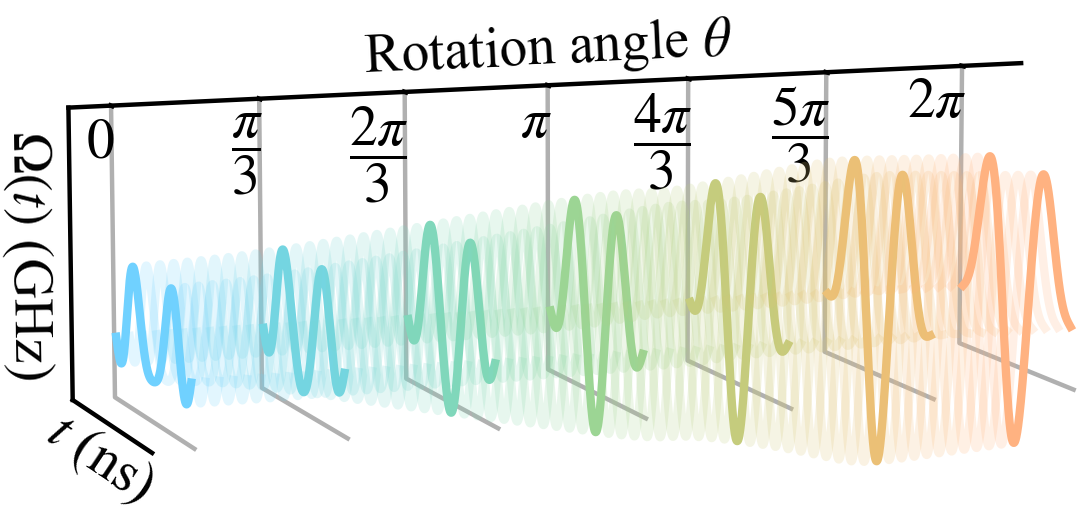
(c)

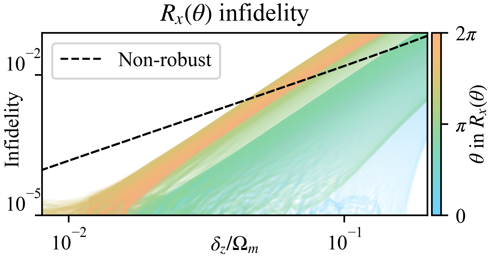
(d)

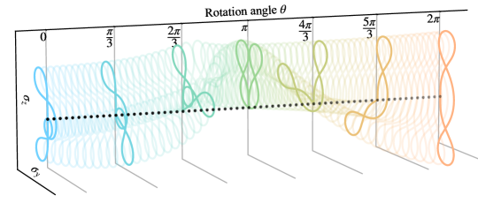
(e)

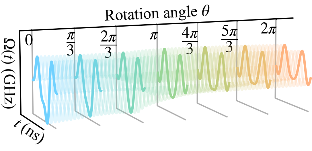
(f)

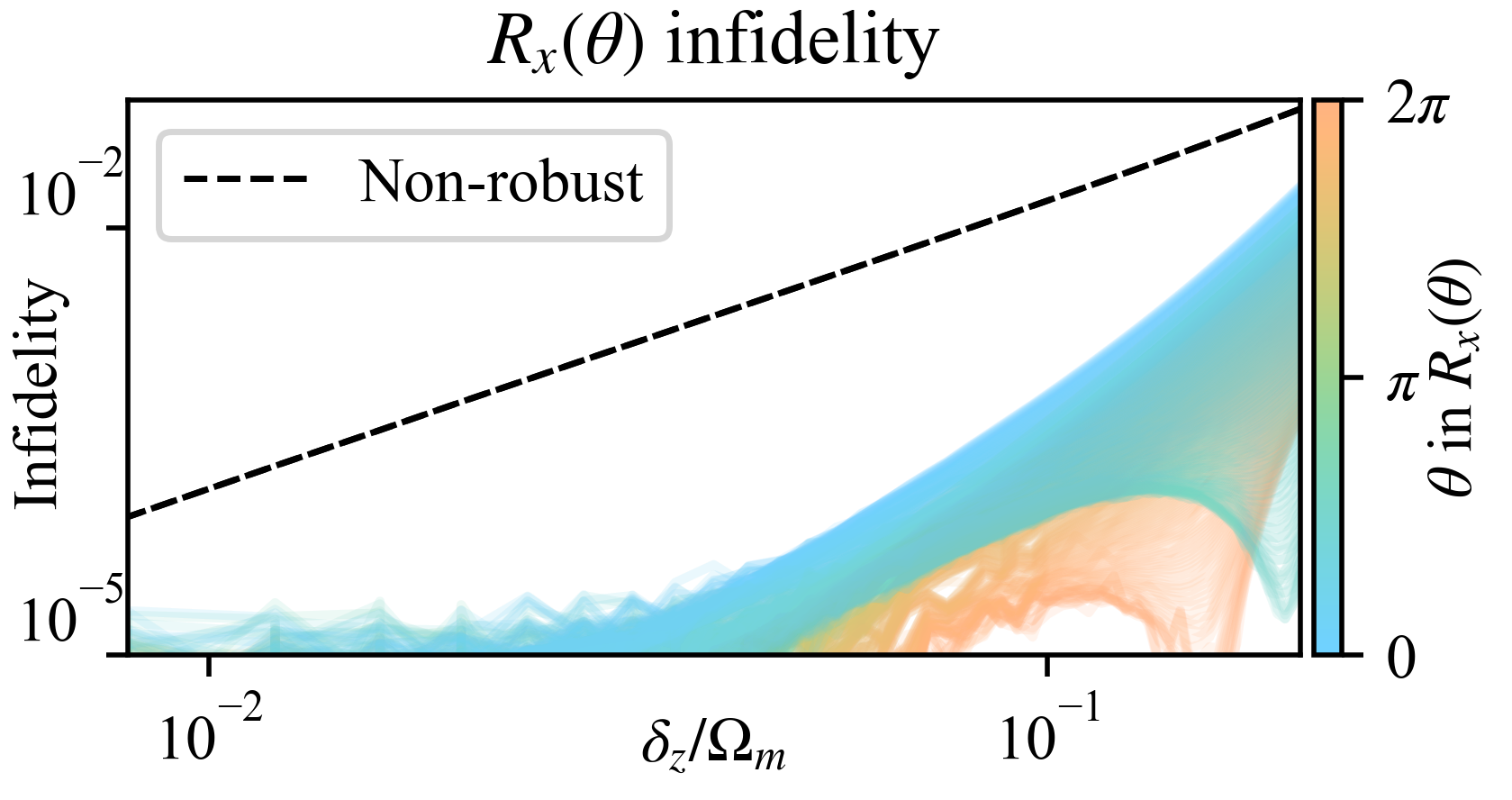
Figure 5: Robust $R_{x}(\theta)$ pulses for $\theta\in[0,2\pi]$, each having 9 parameters, using (a-c) 1st order RIPV with positive $\Delta\theta$ in and (d-f) 2nd order with negative $\Delta\theta$, all variations started from $R_{x}(2\pi)$. In (a-c), global phase $2\pi$ is neglected so $R_{x}(\theta)$ means precisely $R_{x}(\theta+2\pi)$. In each group, on the left we show the QEEDs generated by the pulses. On the right, we show the pulses on the top and fidelity vs noise on the bottom, where $\Omega_{m}$ means the maximum amplitude of the pulse. The fidelity and noise strength are both in logarithm scale with negative $\delta$ mirrored to positive half. Fidelity for curves of different $\theta$ are stacked with transparency. The dashed lines show that for the non-robust $\cos$ pulse implementing $R_{x}(2\pi)$. In all graphs, for visualizing purposes, only about $1/100$ of all pulses are displayed and colors are used uniformly to represent $\theta$.

We can draw several conclusions by observing these graphs. From the QEED graph Figure 5(a), we can see clearly that they all closed at the origin (black dot), indicating that $\mathcal{R}^{1}$ was kept at zero for all $\Omega_{\theta}(t)$ pulses. From Figure 5(b), we see that this series of $R_{x}(\theta)$ pulses are continuously changing with regard to $\theta$. This means we can interpolate between any two pulses to get an intermediate $\theta$ value for $R_{x}(\theta)$. In Figure 5(c), as the variation progresses (with the color changing from blue to orange-red), the fidelity plateau, although narrowing, remains above $0.999$ despite a $5\%$ relative noise. This plateau is ensured because, throughout the variation, $1.414<\mathcal{S}^{1}<1.425$. In contrast, the baseline non-robust pulse has a much higher value of $\mathcal{S}^{1}=21.433$. Furthermore, while the robust pulses maintain a flat response for small $\delta_{z}$ in the log-log infidelity plot, the non-robust pulse shows almost a linear growth.

The 2nd order robustness decreased during variation for we are running the 1st order RIPV. The beginning pulse $\Omega_{0}(t)$ (the left-most blue one in Figure 5(a)) is 2nd-order robust to $\sigma_{z}$ noise. It has $\mathcal{S}^{2}=10.69$, which is small compared to $T^{2}=2500$, resulting in almost zero net area. More directly, if we calculate the 2nd order robustness $\mathcal{R}^{2}=1.18$, we know this pulse cancels approximately $1.18$ digits of $\delta$ to the second order. In Figure 5(c), the first blue curves near $\theta=0$ remained robustness close to $\Omega_{0}(t)$, and possessed similar plateau. As the variation progressed, the 2nd order susceptibility $\mathcal{S}^{2}$ worsened. As a result, the error curves obtained larger positive net area and their infidelity rose fast as $\theta$ goes to $0$ (color changing from blue to orange-red).

2nd order robust $R_{x}(\theta)$.

In the second demonstration, we aim to maintain both 1st and 2nd order robustness. We start from $\Omega_{2\pi}(t)$ and vary backwards to get $\Omega_{\theta}(t)$ for $\theta<2\pi$. The parameters $\mathbf{A}_{2\pi}$ for the beginning pulse is still given by $R_{\text{ex;}\perp}^{2\pi}$ in Hai’s paper [40]. With the same $H_{\text{c}}$ and $H_{\text{n}}$, we only change $\differential{\mathbf{A}}^{\text{pre}}$ and $\Delta\theta_{\text{ideal}}$ to negative values of previous settings. Notice that since we are varying backward this time, we are not neglecting any global phase in discussions.

We can then see from Figure 5(d) that the error curves not only formed closed loops but also maintained zero net area judging by rules of thumb. Quantitatively, all of pulses maintained $1.415<\mathcal{S}^{1}<1.440$ and $10.45<\mathcal{S}^{2}<10.7$, both very small compared to $T=50$ and $T^{2}=2500$. In Figure 5(f), compared to the results of 1st order RIPV, we were able to keep a much wider fidelity plateau as the variation progressed (with color changing from orange-red to blue, since we are decreasing $\theta$ here). The fidelity remained above $0.999$ under $10\%$ noise relative to $\Omega_{m}$. In comparison, the baseline non-robust pulse had $\mathcal{S}^{1}=21.433$ and $\mathcal{S}^{2}=127.7775$ which led to bad fidelity and almost linear growth in log-log scale.

A little compromise of keeping 2nd order robustness, though harmless, is that the dynamics become very complicated, as we can see from the error curves when the pulses are varied towards $\theta=0$. This complicated error curve implies that the trajectories traced by qubits on the Bloch sphere would be convoluted. This complication cannot be overcome because the continuous variation of curves (or homotopy, in mathematical terms) does not change the topology of the error curve. As long as we want to keep the net area close to zero, they are destined to form 3 circular shapes when approaching $\theta=0$.

V.2.2 Multiple noise sources

If there are multiple noise sources, as we discussed in subsubsection IV.3.4, the algorithm is slightly different. To suppress quasi-static noise from all three directions, we need at least 2 independent controls. The rotation angle $\theta_{j}$ on direction $\sigma_{j}$ where $j=x,y,z$ is no longer a simple integration of the pulse, instead, it must be calculated by

$$\theta_{j}=\tr\Big(\sigma_{j}^{\dagger}\big{(}-i\operatorname{logm}U_{\text{sc}}(T)\big{)}\Big{missing})\>,$$

where $\operatorname{logm}$ stands for matrix logarithm. Suppose we want to implement $R_{x}(\theta)$ for convenience. We have to use five constraints $\mathcal{R}_{x},\mathcal{R}_{y},\mathcal{R}_{z},\vartheta_{y}$ and $\vartheta_{z}$ to ensure that the robustness on three axes and the undesired rotations all remain unchanged (variant font $\vartheta$ for undesired rotations).

In this demonstration, we implement $R_{x}(\theta)$ with noises on all three axes and control on two axes, namely

$$H_{\text{c}}(t) =\frac{\Omega_{x}(t)}{2}\sigma_{x}+\frac{\Omega_{y}(t)}{2}\sigma_{y}$$

$$H_{\text{n}} =\delta_{x}\sigma_{x}+\delta_{y}\sigma_{y}+\delta_{z}\sigma_{z}\>.$$

Each pulse is parametrized as Equation 17. We denote $\vec{\Omega}(t)=(\Omega_{x}(t),\Omega_{y}(t))$. The beginning pulse $\vec{\Omega}_{\pi}$, from which we start the variation, implements $R_{x}(\pi)$. The pulse data were given in ref. [40], denoted by $R_{1;\text{all}}^{\pi}$ in the original paper. We used two runs to generate $\vec{\Omega}_{\theta}$ for $\theta\in[0,2\pi]$: one for $\theta\in[\pi,2\pi]$ with $\Delta\theta_{\text{ideal}}>0$ and another for $\theta\in[0,\pi]$ with $\Delta\theta_{\text{ideal}}<0$. The step size was set to

$$\absolutevalue{\Delta\theta_{\text{ideal}}}=5\times 10^{-4}\,\mathrm{rad}\>.$$

For visualization, we only show the pulses and the infidelity-noise graphs in Figure 6, because the error curves are many to visualize. There are now 3 curves for each pulse, each curve being 3D, which means if we project every 3D curve to three 2D axial planes, we would get $3\times 3=9$ curves for each pulse.

(a)

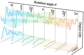
(b)

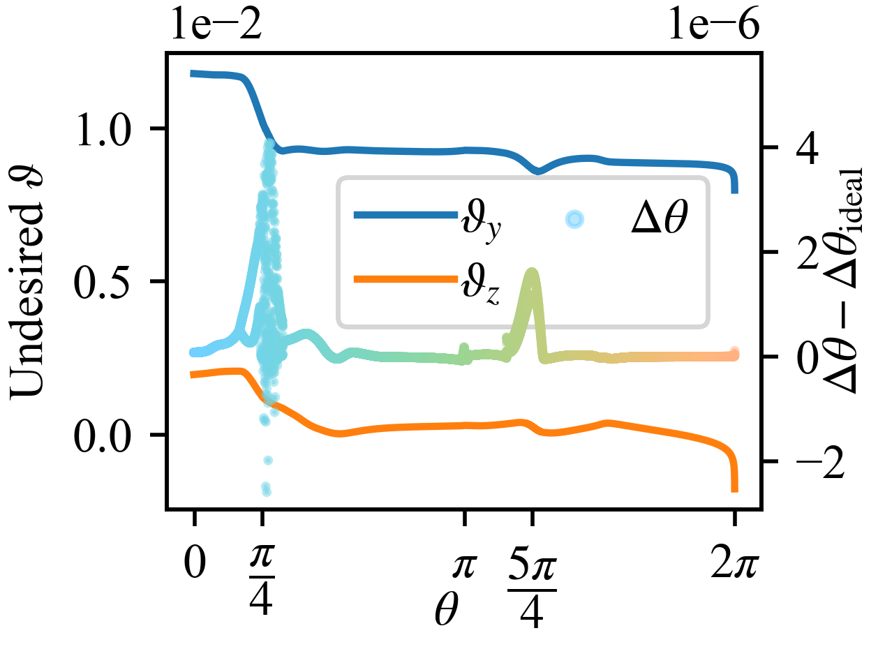
Figure 6: Robust $R_{x}(\theta)$ pulses against noise on $\sigma_{x},\sigma_{y}$ and $\sigma_{z}$, with control $H_{\text{c}}=\frac{\Omega_{x}(t)}{2}\sigma_{x}+\frac{\Omega_{y}(t)}{2}\sigma_{y}$. (a) Pulses as $\theta$ goes from $0$ to $2\pi$. (b) Fidelity vs. noise on three directions, in logarithm scale on both axes and all stacked with transparency. The positive and negative $\delta$ are stacked with the same color, with two ticks at $10^{-2}$ and $10^{-1}$. The black dashed line represents that of the baseline $\sin$ pulse. $\Omega_{m}$ is the maximum pulse amplitude. (c, d) The change of noise susceptibility on three directions and two undesired rotations. The colorful scattered plot (using the y-axis on the right) shows the change of finite difference $\Delta\theta$ on $\sigma_{x}$, relative to the ideal value $\Delta\theta_{\text{ideal}}=5\times 10^{-4}$. In all graphs, for visualizing purposes, only about $1/100$ of all pulses are displayed and colors are used uniformly to represent $\theta$ of $R_{x}(\theta)$.

In Figure 6(a), we see again that the pulses $\Omega_{x}(t)$ (higher) and $\Omega_{y}(t)$ (lower) changed continuously. In Figure 6(b), the infidelity-noise graphs on the three directions, we see that these pulses indeed preserved robustness very well to $\sigma_{y}$ and $\sigma_{z}$. As for $\delta_{x}\sigma_{x}$ noise source, they are robust when $\theta$ is larger than $\pi/4$ (with color from orange-red to green), but the fidelity plateau shrank fast as the variation processes towards $\theta=0$ (colored blue). The worst part is that when there is no noise, the “robust pulses” behaved worse than the non-robust pulse. However, this issue is not a flaw of the algorithm but rather a precision problem, which we believe can be mitigated.

Let’s find out why the fidelity plateau on $\sigma_{x}$ noise shrank very fast. If we plot the 1st order noise susceptibility $\mathcal{S}^{1}_{j}$ on three directions $j=x,y,z$ as a function of $\theta$ in Figure 6(c), we can see that at around $\theta=\pi/4$, the error susceptibility $\mathcal{S}^{1}_{x}$ rose very fast when $\theta$ decreases (recall that for $\theta<\pi$, we decrease $\theta$ during variation). The rise in $\mathcal{S}^{1}_{x}$ theoretically suggests that the fidelity plateau is likely to shrink. The emphasis on likely reflects the uncertainty, as $\mathcal{S}^{1}_{x}$ is only an asymptotic local property defined in the limit $\delta_{x}\to 0$. But why $\mathcal{S}^{1}_{j}$ rose so fast? To understand what happened on the landscape, we plot the deviation of the finite difference $\Delta\theta=\theta(\mathbf{A}+\differential{\mathbf{A}})-\theta(\mathbf{A})$ from its ideal value $\Delta\theta_{\text{ideal}}$ with scatter points and stack it in Figure 6(c). Observe closely the range of $\theta$ where at least one of the 1st order robustness changes, i.e. around $\theta=\pi/4$ and $\theta=5\pi/4$. It is no coincidence that whenever the 1st order robustness changes abruptly, the variation $\Delta\theta$ also deviates sharply (albeit small, at the order of $10^{6}$) around its ideal value ${\Delta\theta}_{\text{ideal}}$. Recall the definition of difference

$$\Delta\theta =\theta(\mathbf{A}+\differential{\mathbf{A}})-\theta(\mathbf{A})$$

$$=\differential{\mathbf{A}}\partialderivative{\theta}{\mathbf{A}}+O(\differential{\mathbf{A}}^{2})$$

$$=\differential{\theta}+O(\differential{\mathbf{A}}^{2})\>.$$

Since in RIPV we require $\differential{\theta}=\Delta\theta_{\text{ideal}}$, the large deviation of $\Delta\theta$ signifies a fact that the landscape $\theta(\mathbf{A})$ is highly nonlinear around those points, i.e. $\Delta\theta-\differential{\theta}\gg 0$. Geometrically, the fast oscillation implies that the level set of the landscape $\theta(\mathbf{A})$ is oscillating about its tangent space.

In summary, the drop in robustness is not a flaw of algorithm design, but is rooted in numerical precision. It can be solved by using smaller $\Delta\theta_{\text{ideal}}$, or by adding an extra optimizing step described in subsubsection IV.4.2 to move the parameter point back on the landscape.

Besides robustness, we can also calculate the undesired rotations $\vartheta_{y}$ and $\vartheta_{z}$ to see why fidelity dropped. We see again in Figure 6(d) that the regions where undesired rotations increase abruptly coincide with those where $\Delta\theta$ significantly deviates from $\Delta\theta_{\text{ideal}}$. This means, at small noise region, the drop of fidelity as $\theta$ approaches $0$ is due to the highly nonlinear nature of the landscapes $\vartheta(\mathbf{A})$ and $\vartheta(\mathbf{A})$.

V.3 Two qubit gates

Implementing two-qubit parametric gates is vital to near term quantum devices, as it provides a threefold reduction in circuit depth as compared to a standard decomposition [42]. We can also use RIPV to get a continuous series of robust two-qubit gates, with only a change of the calculation of rotation angle and adding more undesired rotations to constraints. Here we show a simpler solution.

If we apply the pulse sequence used for $R_{x}(\theta)$ with single $\sigma_{x}$ control, we can achieve a parametric gate generalized from the iSWAP gate, namely the $R_{XY}(\theta)$ gate defined as

$$R_{XY}(\theta)=\exp(-i\frac{\theta}{2}\cdot\frac{\sigma_{x}\sigma_{x}+\sigma_{y}\sigma_{y}}{2})\>,$$

where $\sigma_{x}\sigma_{x}=\sigma_{x}\otimes\sigma_{x}$ is a shorthand for tensor product. In particular, we have $R_{XY}(\frac{\pi}{2})=\textrm{iSWAP}$.

The Hamiltonian for a two-qubit system is

$$H_{0}=\omega_{1}\sigma_{z}I+\omega_{2}I\sigma_{z}+g(\sigma_{x}\sigma_{x}+\sigma_{y}\sigma_{y})\>,$$

where $\omega_{j}$ is the frequency of qubit $j$. Here we only deal with the computational subspace because we would like to separate the effects of leakage from that of coherent noise. To implement an iSWAP gate on superconducting qubits, one could use tunable couplers to make the coupling strength $g$ a driving term $g(t)(\sigma_{x}\sigma_{x}+\sigma_{y}\sigma_{y})$. Hence, we set the control and the noise Hamiltonian as

$$H_{\text{c}}(t) =\frac{\Omega(t)}{2}\cdot\frac{\sigma_{x}\sigma_{x}+\sigma_{y}\sigma_{y}}{2}$$ (18)

$$H_{\text{n}} =\frac{\delta}{2}(\sigma_{z}I-I\sigma_{z})$$ (19)

This $H_{\text{n}}$ signifies the noise on the detuning of two qubits due to frequency shift.

Since both $H_{\text{c}}$ and $H_{\text{n}}$ interact with the subspace spanned by $\{\ket{01},\ket{10}\}$ in the same way as $\sigma_{x}$ and $\sigma_{z}$ interact with $\{\ket{0},\ket{1}\}$, we can use single-qubit $R_{x}(\theta)$ pulses for $\Omega(t)$ in Equation 18 to implement $R_{XY}(\theta)$. The infidelity-noise graph of $R_{XY}(\theta)$ using 2nd order robust pulses obtained in subsubsection V.2.2, is shown in Figure 7. We can see that they are fundamentally the same with the single qubit infidelity curves, except that the calculated infidelity is a little smaller now, since we are considering four levels, namely $\ket{00},\ket{01},\ket{10},\ket{11}$, only half of which are affected by the noise.

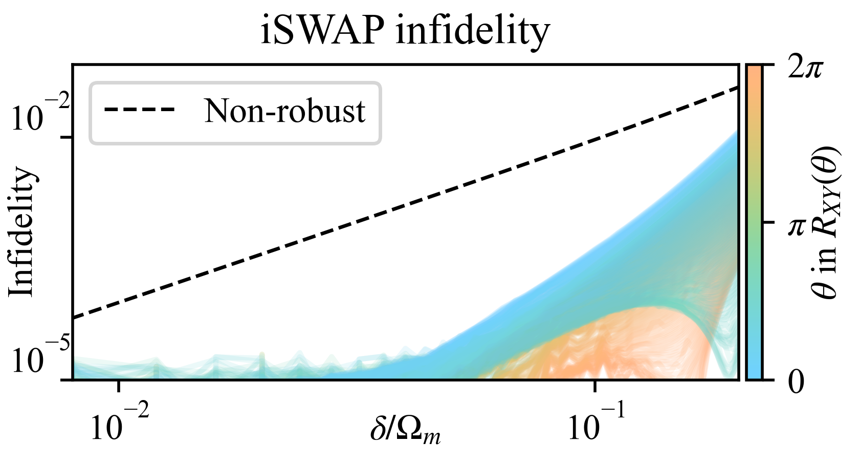
Figure 7: Infidelity-noise graph when using single control pulse sequence for parametric iSWAP gate, or the $R_{XY}(\theta)$ gate.

We emphasize that the RIPV algorithm is not confined to two-dimensional Hilbert space dynamics. By adjusting the calculation of rotation angles and incorporating undesired rotations as constraints, the RIPV algorithm can be adapted for general multi-qubit gates. This allows us to start from a robust pulse sequence for a general multi-qubit gate, which can then be used to generate a continuous series of pulses for parametric multi-qubit gates.

VI Discussion

This work still has many aspects that can be improved or further studied. We list these points here.

To prove of controllability.

We found that by traversing the robustness landscape we can find arbitrary rotational angles, but this doesn’t mean we have full controllability of the quantum systems. To tell whether there is universal robust control over a quantum system, we need to look into the details of how the variation process happens in the QCRL and also examine the properties of the QCRL itself.

To aid multi-objective optimization.

Optimization of multiple objectives is challenging with traditional methods, especially when an aggregated objective function is used. This approach often leads to both objectives changing simultaneously, without control over which one progresses faster or slower. This issue is illustrated in Figure 8 by the blue curve. However, by traversing a level set of one landscape using the GOV algorithm, it is possible to optimize one objective while holding the other constant (the orange zigzag line). This decouples the two objectives, allowing for independent optimization or adjustment.

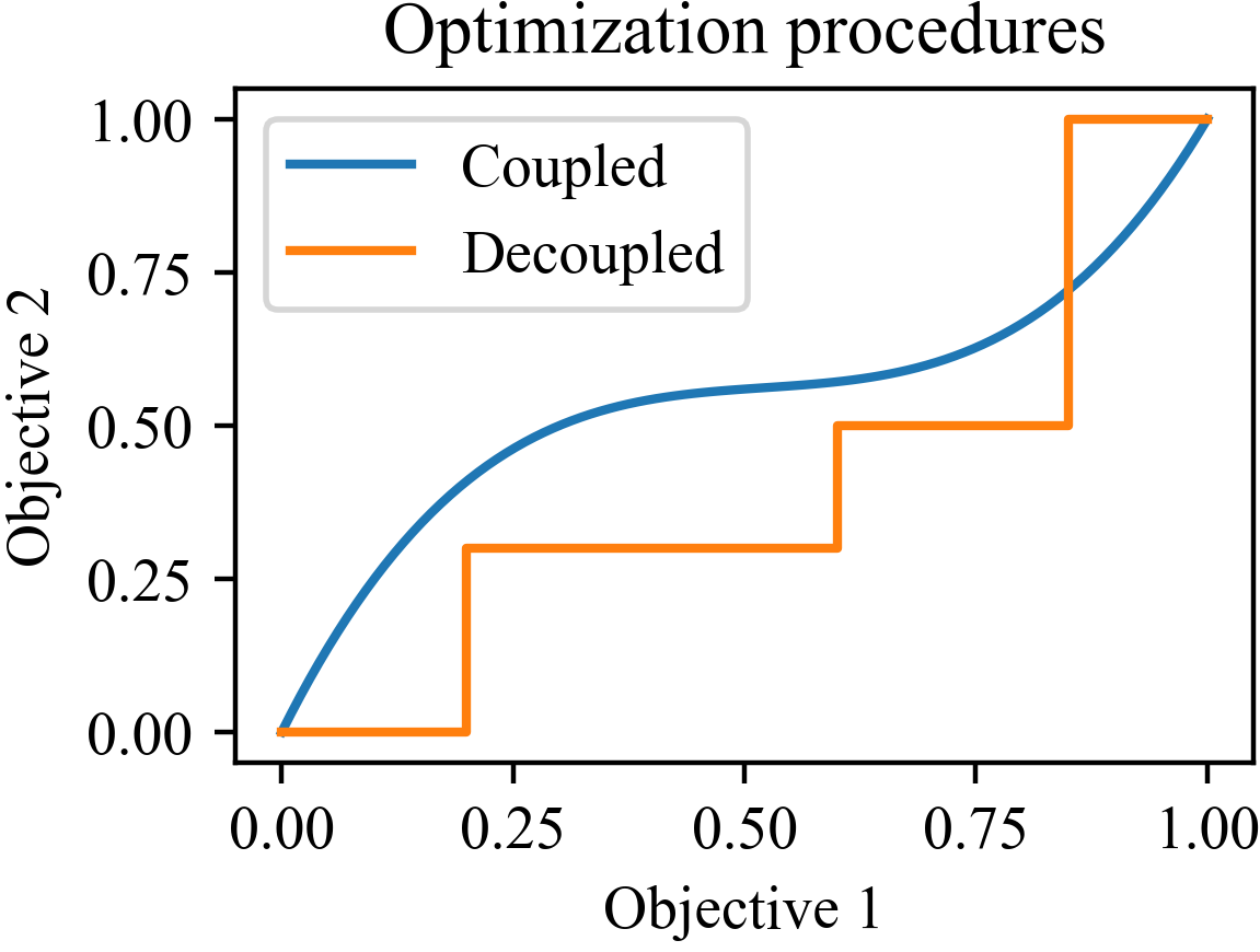
Figure 8: Decoupling two objectives.

To aid robust control.

The shift from QCL to QCRL is more than just a change of the objective function; they are two fundamentally different landscapes. It might be possible to benefit from the landscape structure to speed up the optimization of a robust control, or even find a robust control which was once impossible. An obvious difference is that the QCRL level sets contain robust controls for different ideal gates. We could, for example, start from a robust control of some gate $G_{1}$ and then gradually vary our control to implement another gate $G_{2}$, all while ensuring high robustness. The best part is, we can even insert many optimization runs during the variation process to further ensure robustness. If the QCRL algorithm fails to find a viable variation direction, it is possible that the controls for $G_{1}$ and $G_{2}$ are not in the same connected level set of the QCRL. But if it always finds a viable solution, this solution might be something inaccessible by optimizing the QCL (e.g. we need to go over a hill before reaching globally optimal control).

To include incoherent noise

This work is mainly about coherent noise sources, since we assumed the noise can be expressed as a Hamiltonian $H_{\text{n}}$. However, in most cases, this assumption is just too strong for we can only assume an incoherent noise model. Although when we treat the noise strength as a stochastic parameter, the resulting stochastic Schrödinger equation could model incoherent noise sources, it is still valuable and more straightforward to use some open-system descriptions such as the Lindbladian. Then we have to change the noisy propagator $U_{\text{scn}}$ in Definition 1 to a non-unitary quantum channel, in general a completely positive trace-preserving operator.

VII Conclusion

In this paper, we presented a novel perspective on quantum optimal control tasks, namely the QCRL. Unlike the traditional concept of QCL [4], which is by definition dependent on the specific gate to implement, QCRL emphasizes the effects of noise. The two types of robustness, integral and asymptotic, are defined by either integrating over, or expanding a power series by the noise strength. This approach enables us to find robust control for all tasks within a unified landscape, allowing us to exploit their correlations. Moreover, the level sets of the QCRL offer a rich family of controls, each equally robust against the relevant noise.

Despite being useful, the QCRL still lacks mathematical proof regarding the connectivity of level lets, critical points, and topics similar to that of the QCL. Even the robustness function could be chosen differently, and we did not mention a systematic way on how to choose among those metrics. Further studies of the QCRL could at least prove, hopefully, that its level set is big enough to implement any controllable parametric gate, provided necessary conditions are met.

Building on top of QCRL, we developed a paradigm-shifting algorithm called the RIPV algorithm. As the name suggests, it changes control pulses without undermining robustness. This algorithm is useful to propagate robustness from the control of one gate to a series of others, for example, when implementing a family of parametric gates. We numerically demonstrated on single-qubit and two-qubit parametric gates, with up to two independent control terms. From the QEEDs and infidelity-noise graphs, we can verify that the $R_{x}(\theta)$ fidelity remains at least $0.999$ with $10\%$ noise on $\sigma_{z}$, or at least $0.999$ with $2\%$ noise on three Pauli operators (percentage of pulse maximum amplitude). If we replace robustness or gate parameter with other properties we care about, we can, for example, further optimize gate time, leakage, energy consumption, etc.

At the core of RIPV is the GOV algorithm, a more versatile multipurpose algorithm. Basically, it ensures that, when we vary a point in some landscape, the data point stays in the level set with the freedom of choosing a direction called pre-variation. Choosing the direction that increases (or decreases) the gate parameter gives rise to RIPV. The GOV algorithm brings more than robust quantum control. It allows one to independently change one of many objectives in a multi-objective problem. Through GOV, we can leverage the properties of different landscapes, optimize any one of them without undermining another, and explore their level sets purposefully or randomly.