Movable Antenna-Aided Near-Field Integrated Sensing and Communication

Abstract

Integrated sensing and communication (ISAC) is emerging as a pivotal technology for next-generation wireless networks. However, existing ISAC systems are based on fixed-position antennas (FPAs), which inevitably incur a loss in performance when balancing the trade-off between sensing and communication. Movable antenna (MA) technology offers promising potential to enhance ISAC performance by enabling flexible antenna movement. Nevertheless, exploiting more spatial channel variations requires larger antenna moving regions, which may invalidate the conventional far-field assumption for channels between transceivers. Therefore, this paper utilizes the MA to enhance sensing and communication capabilities in near-field ISAC systems, where a full-duplex base station (BS) is equipped with multiple transmit and receive MAs movable in large-size regions to simultaneously sense multiple targets and serve multiple uplink (UL) and downlink (DL) users for communication. We aim to maximize the weighted sum of sensing and communication rates (WSR) by jointly designing the transmit beamformers, sensing signal covariance matrices, receive beamformers, and MA positions at the BS, as well as the UL power allocation. The resulting optimization problem is challenging to solve, while we propose an efficient two-layer random position (RP) algorithm to tackle it. In addition, to reduce movement delay and cost, we design an antenna position matching (APM) algorithm based on the greedy strategy to minimize the total MA movement distance. Extensive simulation results demonstrate the substantial performance improvement achieved by deploying MAs in near-field ISAC systems. Moreover, the results show the effectiveness of the proposed APM algorithm in reducing the antenna movement distance, which is helpful for energy saving and time overhead reduction for MA-aided near-field ISAC systems with large moving regions.

I Introduction

Integrated sensing and communication (ISAC) has been considered as a promising technology for next-generation wireless networks because of its unique ability to efficiently reuse time, frequency, power, and hardware resources for both sensing and communication tasks at the same time [1, 2]. In addition, the continuous and aggressive utilization of frequency spectrum, such as millimeter-wave (mmWave), in wireless communications has resulted in spectrum overlap with conventional radar systems, thereby driving the need for the development of ISAC frameworks [3].

In the ISAC system, one key challenge is to design dual-functional signals that can achieve both the sensing and communication tasks. It is worth noting that multiple-input multiple-output (MIMO) technology provides a viable solution to this issue by exploiting spatial degrees of freedom (DoFs) through beamforming design. Specifically, MIMO-based ISAC systems, equipped with multiple antennas at both the transmitter and receiver, can employ beamforming to steer the sensing/communication signals toward the desired targets/users, which reduces interference in undesired directions and enhances the quality of ISAC performance [4]. Motivated by this, substantial works have explored beamforming design in MIMO-based wireless sensing and communication systems [5, 6, 7, 8, 9, 10, 11]. However, most existing ISAC systems focus on either uplink (UL) or downlink (DL) communication, which cannot simultaneously meet both communication demands, thus incurring reduced system throughput. To address this limitation, full-duplex ISAC systems have been proposed [12], which enable simultaneous transmission and reception of sensing/communication signals over the same frequency. The full-duplex operation improves both sensing and communication capabilities through the efficient reuse of time-frequency resources. In terms of sensing, the entire frequency bands are available to detect targets such that an enhanced radar performance is achieved. From the communication perspective, there is a significant improvement in spectral efficiency [12]. Accordingly, full-duplex ISAC systems have garnered significant attention [13, 14, 15]. The authors in [13] investigated the joint secure transceiver design for the full-duplex ISAC system, where the base station (BS) simultaneously performs target tracking and communicates with the UL and DL users. The authors in [14] studied the joint optimization of a full-duplex communication-based ISAC system under the criteria of transmit power minimization and sum-rate maximization. The results demonstrated the performance gains in terms of both the power and the spectral efficiency compared to the conventional half-duplex ISAC. More comprehensively, the authors in [15] compared the different advantages of ISAC systems operating in full-duplex and half-duplex modes.

However, conventional ISAC architectures mentioned above typically utilize fixed-position antenna (FPA) arrays, which limit the exploitation of spatial DoFs available in the continuous spatial domain. This limitation hinders the ability to fully optimize spatial diversity and multiplexing performance in sensing and communication tasks, thus constraining the overall potential of ISAC systems [16]. Fortunately, movable antenna (MA) and six-dimensional MA (6DMA) technologies have recently been proposed to address this limitation [17, 18, 19, 20, 21, 22]. Specifically, MA technology can adjust antenna positions on a line/surface with fixed antenna rotation to effectively provide customized sensing and communication services [17, 18]. More generally, 6DMA technology can incorporate the DoFs in the three-dimensional (3D) position and 3D orientation/rotation of antennas, which can adaptively allocate antenna resources based on the long-term/statistical user distribution to improve network capacity [19, 20, 21, 22]. The various wireless sensing/ISAC systems applying MA have been extensively studied recently [23, 24, 25]. The authors in [23] analyzed the performance of a new wireless sensing system equipped with a one-dimensional (1D) or two-dimensional (2D) array. The authors in [24] minimized the Cramér-Rao bound (CRB) through the joint beamforming design and MA position optimization. Moreover, the authors in [25] proposed a 6DMA-aided wireless sensing system and compared it with MA for both directive and isotropic antenna radiation patterns. In addition, based on previous studies of MA-aided full-duplex wireless communication systems [26, 27, 28, 29], the full-duplex ISAC system aided by MAs has begun to attract the attention of researchers [30, 31, 32]. The authors in [30] focused on maximizing the communication rate and sensing mutual information in a monostatic MA-ISAC system. The authors in [31] investigated the joint discrete antenna positioning and beamforming optimization in MA-enabled full-duplex ISAC networks. The authors in [32] considered the joint active beamforming and position coefficients design problem in an MA-aided networked full-duplex ISAC system that accomplishes radar sensing as well as UL and DL communication capabilities concurrently.

While the advantages of MA in ISAC systems have been validated, existing studies mainly focus on far-field ISAC systems. Generally, to accommodate the free movement of multiple MAs and maximize spatial DoFs, larger antenna moving regions are required [33, 34]. Hence, the MA system usually has a larger aperture size compared to conventional FPA-based systems. Besides, to meet the ever-growing demands for sensing and communication performance, future ISAC systems are expected to operate in high-frequency bands [35]. The above two reasons render the conventional far-field assumption commonly adopted in previous MA-aided ISAC systems invalid. As a result, it is essential to explore the potential advantages that MA can offer to ISAC systems in near-field scenarios. It is noteworthy that the additional distance dimension in near-field ISAC compared to far-field ISAC allows the system to provide sensing/communication services for multiple targets/users through joint resolutions in both the angle and distance domains [36, 37]. However, to the best of the authors’ knowledge, there has been no prior work on designing MA-aided ISAC systems under near-field channel conditions and optimizing the corresponding system performance. Therefore, in this paper, we investigate MA-aided near-field ISAC systems. The main contributions of this paper are summarized as follows:

• We propose an MA-aided ISAC system that employs the near-field spherical wave channel model, where the dual-functional full-duplex BS is equipped with multiple transmit and receive MAs movable in large-size regions to simultaneously sense multiple targets and serve multiple UL and DL users for communication. To balance sensing accuracy and communication efficiency, we aim to maximize the weighted sum of sensing and communication rates (WSR) by jointly designing the transmit beamformers, sensing signal covariance matrices, receive beamformers, and MA positions at the BS, as well as the UL power allocation.

• We propose a two-layer random position (RP) algorithm to solve the formulated non-convex optimization problem with highly-coupled variables. In the inner-layer, for a given MA position, we iteratively update the remaining optimization variables based on the alternating optimization (AO) framework. In the outer-layer, we randomly assign multiple pairs of transmit and receive MA positions and select the pair that maximizes the WSR. Moreover, to reduce the overhead associated with the real-time movement of multiple MAs within the large-size moving region, we propose an antenna position matching (APM) algorithm that effectively minimizes the total MA movement distance.

• We conduct extensive simulations to validate the advantages of MA-aided near-field ISAC systems and the effectiveness of the proposed algorithms. The results demonstrate that the MA-aided ISAC system outperforms the ISAC system based on FPAs due to the additional DoFs introduced by antenna position optimization. In addition, a larger moving region for MAs increases the equivalent array aperture, thus providing an efficient way to enlarge the near-field region of ISAC systems without increasing the number of antennas, which facilitates multi-location beamfocusing. Furthermore, the proposed APM algorithm effectively reduces the total MA movement distance, which significantly reduces the energy consumption and time overhead for antenna movement in practical systems.

The rest of this paper is organized as follows. Section II introduces the system model and the optimization problem for the proposed system. In Section III, we propose the two-layer RP algorithm and APM algorithm to solve the optimization problem and minimize the total MA movement distance, respectively. Next, simulation results and discussions are provided in Section IV. Finally, this paper is concluded in Section V.

Notation: $a/A$, $\mathbf{a}$, $\mathbf{A}$, and $\mathcal{A}$ denote a scalar, a vector, a matrix, and a set, respectively. $A!$ represents the factorial of positive integer $A$. $\mathbf{A}\succeq\mathbf{0}$ indicates that $\mathbf{A}$ is a positive semidefinite matrix. ${\left(\cdot\right)^{T}}$, ${\left(\cdot\right)^{H}}$, $\left\|\cdot\right\|_{2}$, $\left|\cdot\right|$, $\mathrm{Tr}\left\{\cdot\right\}$, and $\mathrm{Rank}\left\{\cdot\right\}$ denote the transpose, conjugate transpose, Euclidean norm, absolute value, trace, and rank, respectively. $\mathbb{C}^{M\times N}$ and $\mathbb{R}^{M\times N}$ are the sets for complex and real matrices of $M\times N$ dimensions, respectively. $\mathbf{I}_{N}$ is the identity matrix of order $N$. $\mathcal{CN}\left(\mathbf{0},\mathbf{\Lambda}\right)$ represents the circularly symmetric complex Gaussian (CSCG) distribution with mean zero and covariance matrix $\mathbf{\Lambda}$. $\mathcal{A}\backslash\mathcal{B}$ denotes the subtraction of set $\mathcal{B}$ from set $\mathcal{A}$.

II System Model and Problem Formulation

Figure 1: Illustration of the proposed MA-aided near-field ISAC system.

Consider an MA-aided near-field ISAC system as shown in Fig. 1, where a dual-functional full-duplex BS equipped with two MA arrays transmits the DL ISAC signal and receives the UL communication signal from $J$ single-FPA half-duplex UL users, along with the reflected ISAC signal from sensing targets, via the same time-frequency resource. The DL ISAC signal is transmitted from the $N$-element MA array to simultaneously communicate with $K$ single-FPA half-duplex DL users and detect $L$ point sensing targets. The sensing echo signal and the UL communication signal are received at the BS through the receive MA array equipped with $M$ elements. Each transmit or receive MA can move freely within its designated transmit or receive region, i.e., $\mathcal{C}_{\mathrm{t}}$ or $\mathcal{C}_{\mathrm{r}}$, respectively. Without loss of generality, we assume that the targets and users are located within the BS’s near-field region.

II-A Channel Model

We consider the quasi-static near-field spherical wave channel model [33, 34] for the self-interference (SI) channel, communication channel, and sensing channel. Since these channels can be actively reconfigured through MA movement, we establish a global Cartesian coordinate system $o$-$xyz$ at the BS to describe the MA positions with the reference point between the transmit and receive regions defined as origin $o$, where axes $x$ and $y$ are defined as the horizontal and vertical directions in the MA array plane, respectively, and axis $z$ is perpendicular to the array plane (see Fig. 1). The coordinates of $N$ transmit MAs and $M$ receive MAs are described by $\mathbf{t}={\left[{\mathbf{t}_{1}^{T},\ldots,\mathbf{t}_{N}^{T}}\right]^{T}}\in{\mathbb{R}^{3N\times 1}}$ and $\mathbf{r}={\left[{\mathbf{r}_{1}^{T},\ldots,\mathbf{r}_{M}^{T}}\right]^{T}}\in{\mathbb{R}^{3M\times 1}}$, where ${\mathbf{t}_{n}}=\left[{x_{n}^{\mathrm{t}},y_{n}^{\mathrm{t}},0}\right]^{T}\in\mathcal{C}_{\mathrm{t}}$ ($1\leq n\leq N$) and ${\mathbf{r}_{m}}=\left[{x_{m}^{\mathrm{r}},y_{m}^{\mathrm{r}},0}\right]^{T}\in\mathcal{C}_{\mathrm{r}}$ ($1\leq m\leq M$), respectively. The coordinates of UL user $j$ ($j\in\mathcal{J}=\left\{{1,\ldots,J}\right\}$), DL user $k$ ($k\in\mathcal{K}=\left\{{1,\ldots,K}\right\}$), and target $l$ ($l\in\mathcal{L}=\left\{{1,\ldots,L}\right\}$) are denoted as $\mathbf{q}_{\mathrm{U}_{j}}\in\mathbb{R}^{3\times 1}$, $\mathbf{q}_{\mathrm{D}_{k}}\in\mathbb{R}^{3\times 1}$, and $\mathbf{q}_{\mathrm{S}_{l}}\in\mathbb{R}^{3\times 1}$, respectively.

According to the spherical wave model, the SI channel is given by

$${\mathbf{H}_{\mathrm{SI}}}\left(\mathbf{t},\mathbf{r}\right)$$

$$=\rho_{\mathrm{SI}}\left[{\begin{array}[]{*{20}{c}}{{e^{\mathrm{j}\frac{{2\pi}}{\lambda}{{\left\|{{\mathbf{t}_{1}}-{\mathbf{r}_{1}}}\right\|}_{2}}}}}&\ldots&{{e^{\mathrm{j}\frac{{2\pi}}{\lambda}{{\left\|{{\mathbf{t}_{N}}-{\mathbf{r}_{1}}}\right\|}_{2}}}}}\\ \vdots&\vdots&\vdots\\ {{e^{\mathrm{j}\frac{{2\pi}}{\lambda}{{\left\|{{\mathbf{t}_{1}}-{\mathbf{r}_{M}}}\right\|}_{2}}}}}&\ldots&{{e^{\mathrm{j}\frac{{2\pi}}{\lambda}{{\left\|{{\mathbf{t}_{N}}-{\mathbf{r}_{M}}}\right\|}_{2}}}}}\end{array}}\right]\in\mathbb{C}^{M\times N},$$ (4)

where $\lambda$ is the carrier wavelength and $0<\rho_{\mathrm{SI}}\ll 1$ is the SI loss coefficient representing the path loss and the SI cancellations in analog and digital domains. The DL user $k$’s and UL user $j$’s communication channels can be respectively expressed as the functions of the transmit and receive MAs’ position vectors, i.e.,

$${\mathbf{h}_{k}}\left(\mathbf{t}\right)={\rho_{{\mathrm{D}_{k}}}}{\left[{{e^{\mathrm{j}\frac{{2\pi}}{\lambda}{{\left\|{{\mathbf{t}_{1}}-{\mathbf{q}_{{\mathrm{D}_{k}}}}}\right\|}_{2}}}},\ldots,{e^{\mathrm{j}\frac{{2\pi}}{\lambda}{{\left\|{{\mathbf{t}_{N}}-{\mathbf{q}_{{\mathrm{D}_{k}}}}}\right\|}_{2}}}}}\right]^{T}}\in\mathbb{C}^{N\times 1},$$ (5)

$${\mathbf{f}_{j}}\left(\mathbf{r}\right)={\rho_{{\mathrm{U}_{j}}}}{\left[{{e^{\mathrm{j}\frac{{2\pi}}{\lambda}{{\left\|{{\mathbf{r}_{1}}-{\mathbf{q}_{{\mathrm{U}_{j}}}}}\right\|}_{2}}}},\ldots,{e^{\mathrm{j}\frac{{2\pi}}{\lambda}{{\left\|{{\mathbf{r}_{M}}-{\mathbf{q}_{{\mathrm{U}_{j}}}}}\right\|}_{2}}}}}\right]^{T}}\in\mathbb{C}^{M\times 1},$$ (6)

where ${\rho_{{\mathrm{D}_{k}}}}$ and ${\rho_{{\mathrm{U}_{j}}}}$ accounts for the corresponding path loss.

For the sensing channel of target $l$, we denote the transmit near-field response vector by

$${\mathbf{g}_{\mathrm{t},l}}\left(\mathbf{t}\right)={\left[{{e^{\mathrm{j}\frac{{2\pi}}{\lambda}{{\left\|{{\mathbf{t}_{1}}-{\mathbf{q}_{{\mathrm{S}_{l}}}}}\right\|}_{2}}}},\ldots,{e^{\mathrm{j}\frac{{2\pi}}{\lambda}{{\left\|{{\mathbf{t}_{N}}-{\mathbf{q}_{{\mathrm{S}_{l}}}}}\right\|}_{2}}}}}\right]^{T}}\in\mathbb{C}^{N\times 1},$$ (7)

and similarly denote by

$${\mathbf{g}_{\mathrm{r},l}}\left(\mathbf{r}\right)={\left[{{e^{\mathrm{j}\frac{{2\pi}}{\lambda}{{\left\|{{\mathbf{r}_{1}}-{\mathbf{q}_{{\mathrm{S}_{l}}}}}\right\|}_{2}}}},\ldots,{e^{\mathrm{j}\frac{{2\pi}}{\lambda}{{\left\|{{\mathbf{r}_{M}}-{\mathbf{q}_{{\mathrm{S}_{l}}}}}\right\|}_{2}}}}}\right]^{T}}\in\mathbb{C}^{M\times 1},$$ (8)

the receive near-field response vector. The target $l$’s sensing channel is thus given by $\mathbf{G}_{l}\left(\mathbf{t},\mathbf{r}\right)={\rho_{{\mathrm{S}_{l}}}}{\mathbf{g}_{\mathrm{r},l}}\left(\mathbf{r}\right){\mathbf{g}_{\mathrm{t},l}}\left(\mathbf{t}\right)^{H}\in\mathbb{C}^{M\times N}$, where ${\rho_{{\mathrm{S}_{l}}}}$ is the round-trip channel coefficient determined by the path loss and the radar cross-section of the target.

II-B Signal Model

We first focus on the DL ISAC signal used for simultaneous sensing and DL multi-user communication via $N$-element MA array beamforming, which is expressed as

$$\mathbf{x}=\sum\limits_{l\in\mathcal{L}}{{\mathbf{s}_{l}}}+\sum\limits_{k\in\mathcal{K}}{{\mathbf{w}_{k}}{d_{{\mathrm{D}_{k}}}}}\in\mathbb{C}^{N\times 1},$$ (9)

where $\mathbf{w}_{k}\in\mathbb{C}^{N\times 1}$ is the beamformer of DL user $k$ and ${d_{{\mathrm{D}_{k}}}}$ is the corresponding DL signal with normalized power, i.e., $\mathbb{E}\left\{{{{\left|{{d_{{\mathrm{D}_{k}}}}}\right|}^{2}}}\right\}=1$. $\mathbf{s}_{l}\in\mathbb{C}^{N\times 1}$ is the dedicated sensing signal for target $l$ with the covariance matrix ${\mathbf{S}_{l}}=\mathbb{E}\left\{{{\mathbf{s}_{l}}\mathbf{s}_{l}^{H}}\right\}\in\mathbb{C}^{N\times N}$. Here, we assume that the signals $d_{{\mathrm{D}_{k}}}$ and $\mathbf{s}_{l}$ are independent of each other. The received signal at DL user $k$ is given by

$${y_{k}}=\underbrace{\mathbf{h}_{k}^{H}{\mathbf{w}_{k}}{d_{{\mathrm{D}_{k}}}}}_{\mathrm{Desired\ siganl}}+\underbrace{\sum\limits_{i\in\mathcal{K}\backslash k}{\mathbf{h}_{k}^{H}{\mathbf{w}_{i}}{d_{{\mathrm{D}_{i}}}}}}_{\mathrm{Multi-user\ interference}}+\underbrace{\sum\limits_{l\in\mathcal{L}}{\mathbf{h}_{k}^{H}{\mathbf{s}_{l}}}}_{\mathrm{Sensing\ signal}}+{n_{k}},$$ (10)

where $n_{k}\sim\mathcal{CN}\left(0,\sigma^{2}_{k}\right)$ represents the additive white Gaussian noise (AWGN) with zero mean and variance $\sigma^{2}_{k}$.

As the full-duplex BS transmits the DL ISAC signal, it simultaneously receives the UL communication signal and the target reflection. Denote the signal from UL user $j$ by ${d_{{\mathrm{U}_{j}}}}$, which satisfies $\mathbb{E}\left\{{{{\left|{{d_{{\mathrm{U}_{j}}}}}\right|}^{2}}}\right\}=1$. The received signal at the full-duplex BS can be expressed as

$${\mathbf{y}_{\mathrm{BS}}}=\underbrace{\sum\limits_{j\in\mathcal{J}}{{\mathbf{f}_{j}}\sqrt{{p_{j}}}{d_{{\mathrm{U}_{j}}}}}}_{\mathrm{Communication\ signal}}+\underbrace{\sum\limits_{l\in\mathcal{L}}{{\mathbf{G}_{l}}\mathbf{x}}}_{\mathrm{Target\ reflection}}+\underbrace{{\mathbf{H}_{\mathrm{SI}}}\mathbf{x}}_{\mathrm{SI}}+{\mathbf{n}_{\mathrm{BS}}},$$ (11)

where $p_{j}$ is the transmit power of UL user $j$, ${\mathbf{n}_{\mathrm{BS}}}\sim\mathcal{CN}\left(\mathbf{0},\sigma^{2}_{\mathrm{BS}}\mathbf{I}_{M}\right)$ is the AWGN at the BS with zero mean and variance $\sigma^{2}_{\mathrm{BS}}$.

II-C Sensing and Communication Performance Metrics

The BS uses the received signal (11) to sense the target. When considering point target detection in MIMO radar systems, the detection probability of target $l$ is generally a monotonically increasing function of the output signal-to-interference-plus-noise ratio (SINR) [8, 14]. To capture the reflected signal of target $l$, the BS applies the receive beamformer, $\mathbf{u}_{l}\in\mathbb{C}^{M\times 1}$, on received signal ${\mathbf{y}_{\mathrm{BS}}}$, and thus the corresponding SINR is given by

$${{\gamma}_{{\mathrm{S}_{l}}}}=\frac{{\mathbf{u}_{l}^{H}{\mathbf{G}_{l}}\mathbf{R}\mathbf{G}_{l}^{H}{\mathbf{u}_{l}}}}{{\mathbf{u}_{l}^{H}\left({\sum\limits_{j\in\mathcal{J}}{{p_{j}}{\mathbf{f}_{j}}\mathbf{f}_{j}^{H}}+{\mathbf{A}_{l}}\mathbf{R}\mathbf{A}_{l}^{H}+\sigma_{\mathrm{BS}}^{2}{\mathbf{I}_{M}}}\right){\mathbf{u}_{l}}}},$$ (12)

where $\mathbf{R}=\mathbb{E}\left\{{\mathbf{x}{\mathbf{x}^{H}}}\right\}=\sum\nolimits_{l\in\mathcal{L}}{{\mathbf{S}_{l}}}+\sum\nolimits_{k\in\mathcal{K}}{{\mathbf{w}_{k}}\mathbf{w}_{k}^{H}}\in\mathbb{C}^{N\times N}$ and $\mathbf{A}_{l}=\sum\nolimits_{i\in\mathcal{L}\backslash l}{{\mathbf{G}_{i}}}+{\mathbf{H}_{\mathrm{SI}}}\in\mathbb{C}^{M\times N}$. To mathematically align with the logarithmic form of the communication rate, sensing performance is assessed using sensing rate, i.e., $R_{{\mathrm{S}_{l}}}=\log_{2}\left(1+{\gamma_{{\mathrm{S}_{l}}}}\right)$, like in [11, 16, 30, 37]. The optimal sensing waveform designed to maximize the sensing rate has the same estimation performance as the optimal sensing waveform designed to minimize the mean-square error in estimating the target sensing response $\mathbf{G}_{l}$ [11].

Similarly, the BS applies another set of receive beamformers, $\mathbf{b}_{j}\in\mathbb{C}^{M\times 1}$, on ${\mathbf{y}_{\mathrm{BS}}}$ to decode the data signal of UL user $j$. The corresponding UL communication rate is given by $R_{{\mathrm{U}_{j}}}=\log_{2}\left(1+{\gamma_{{\mathrm{U}_{j}}}}\right)$, where ${\gamma_{{\mathrm{U}_{j}}}}$ is the receive SINR given by

$${{\gamma}_{{\mathrm{U}_{j}}}}=\frac{{{p_{j}}\mathbf{b}_{j}^{H}{\mathbf{f}_{j}}\mathbf{f}_{j}^{H}{\mathbf{b}_{j}}}}{{\mathbf{b}_{j}^{H}\left({\sum\limits_{i\in\mathcal{J}\backslash j}{{p_{i}}{\mathbf{f}_{i}}\mathbf{f}_{i}^{H}}+\mathbf{A}\mathbf{R}{\mathbf{A}^{H}}+\sigma_{\mathrm{BS}}^{2}{\mathbf{I}_{M}}}\right){\mathbf{b}_{j}}}},$$ (13)

where $\mathbf{A}=\sum\nolimits_{l\in\mathcal{L}}{{\mathbf{G}_{l}}}+{\mathbf{H}_{\mathrm{SI}}}\in\mathbb{C}^{M\times N}$. For DL communication, (10) indicates that the SINR of DL user $k$ can be expressed as

$${\gamma_{{\mathrm{D}_{k}}}}=\frac{{{{\left|{\mathbf{h}_{k}^{H}{\mathbf{w}_{k}}}\right|}^{2}}}}{{\sum\limits_{i\in\mathcal{K}\backslash k}{{{\left|{\mathbf{h}_{k}^{H}{\mathbf{w}_{i}}}\right|}^{2}}}+\sum\limits_{l\in\mathcal{L}}{\mathbf{h}_{k}^{H}{\mathbf{S}_{l}}{\mathbf{h}_{k}}}+\sigma_{k}^{2}}},$$ (14)

and the corresponding DL communication rate is given by $R_{{\mathrm{D}_{k}}}=\log_{2}\left(1+{\gamma_{{\mathrm{D}_{k}}}}\right)$.

II-D Problem Formulation

Herein, we aim to maximize the WSR to balance sensing accuracy and communication efficiency, which can be expressed as

$$WSR=\sum\limits_{l\in\mathcal{L}}{{\varpi_{{\mathrm{S}_{l}}}}{R_{{\mathrm{S}_{l}}}}}+\sum\limits_{j\in\mathcal{J}}{{\varpi_{{\mathrm{U}_{j}}}}{R_{{\mathrm{U}_{j}}}}}+\sum\limits_{k\in\mathcal{K}}{{\varpi_{{\mathrm{D}_{k}}}}{R_{{\mathrm{D}_{k}}}}},$$ (15)

where ${\varpi_{{\mathrm{S}_{l}}}}\geq 0$, ${\varpi_{{\mathrm{U}_{j}}}}\geq 0$, and ${\varpi_{{\mathrm{D}_{k}}}}\geq 0$ denote predefined rate weights for target $l$, UL user $j$, and DL user $k$, respectively, which satisfy $\sum\nolimits_{l\in\mathcal{L}}{{\varpi_{{\mathrm{S}_{l}}}}}+\sum\nolimits_{j\in\mathcal{J}}{{\varpi_{{\mathrm{U}_{j}}}}}+\sum\nolimits_{k\in\mathcal{K}}{{\varpi_{{\mathrm{D}_{k}}}}}=1$ and can be used to prioritize the targets and users. In particular, we jointly optimize the receive beamformers, $\mathbf{u}_{l}$ and $\mathbf{b}_{j}$, sensing signal covariance matrices, $\mathbf{S}_{l}$, transmit beamformers, $\mathbf{w}_{k}$, UL transmit power, $p_{j}$, and MA positions, $\mathbf{t}$ and $\mathbf{r}$. The corresponding problem is formulated as

$$\mathop{\mathrm{maximize}}\limits_{\mathbf{u}_{l},\mathbf{b}_{j},\mathbf{S}_{l},\mathbf{w}_{k},p_{j},\mathbf{t},\mathbf{r}}\quad WSR$$ (16)

$$\mathrm{s.t.}\quad\mathrm{C1}:\left\|{\mathbf{u}_{l}}\right\|_{2}^{2}=1,\ \forall{l}\in\mathcal{L},$$

$$\hskip 23.00006pt\mathrm{C2}:\left\|{\mathbf{b}_{j}}\right\|_{2}^{2}=1,\ \forall{j}\in\mathcal{J},$$

$$\hskip 23.00006pt\mathrm{C3}:\sum\limits_{l\in{\mathcal{L}}}{\mathrm{Tr}\left\{\mathbf{S}_{l}\right\}}+\sum\limits_{k\in{\mathcal{K}}}{\left\|{\mathbf{w}_{k}}\right\|_{2}^{2}}\leq P_{\mathrm{D}}^{\mathrm{max}},$$

$$\hskip 23.00006pt\mathrm{C4}:0\leq{p_{j}}\leq P_{\mathrm{U}}^{\mathrm{max}},\ \forall j\in\mathcal{J},$$

$$\hskip 23.00006pt\mathrm{C5}:\mathbf{t}\in{\mathcal{C}_{\mathrm{t}}},\ \mathbf{r}\in{\mathcal{C}_{\mathrm{r}}},$$

$$\hskip 23.00006pt\mathrm{C6}:{\left\|{{\mathbf{t}_{a}}-{\mathbf{t}_{\tilde{a}}}}\right\|_{2}}\geq D,\ 1\leq a\neq{\tilde{a}}\leq N,$$

$$\hskip 23.00006pt\mathrm{C7}:{\left\|{{\mathbf{r}_{b}}-{\mathbf{r}_{\tilde{b}}}}\right\|_{2}}\geq D,\ 1\leq b\neq{\tilde{b}}\leq M.$$

Here, constraints C1 and C2 normalize the receive beamformers. Constraints C3 and C4 indicate that the total transmit powers of DL and UL transmissions should not exceed the maximum limits, $P_{\mathrm{D}}^{\mathrm{max}}$ and $P_{\mathrm{U}}^{\mathrm{max}}$, respectively. Constraint C5 confines the moving regions of transmit and receive MAs. Constraints C6 and C7 ensure the minimum inter-MA distance, $D$, at the BS for practical implementation. Note that problem (16) is a non-convex optimization problem with coupled variables, and thus finding globally optimal solutions for it in polynomial time is challenging. Thus, we develop an efficient two-layer RP algorithm to obtain suboptimal solutions for this problem in the next section.

III Proposed Solution

The AO algorithm is commonly used to solve optimization problems in wireless communication systems. It decomposes the original problem into manageable sub-problems and iteratively solves each one while keeping the optimization variables of other sub-problems fixed. For MA-aided communication systems, a straightforward approach is to separate the optimization of MA positions and other variables into two independent problems and then solve them iteratively [17]. However, the conventional AO algorithm may converge to undesired local optimal solutions because the MA positions (or other variables) determined in the previous iteration restrict the optimization space for other variables (or MA positions) in the current iteration [38]. Therefore, we propose a two-layer RP algorithm. In the inner-layer, for a given MA position, we decompose problem (16) into two sub-problems, i.e., iteratively updating $\left\{\mathbf{u}_{l},\mathbf{b}_{j}\right\}$ with closed-form expressions and $\left\{\mathbf{S}_{l},\mathbf{w}_{k},p_{j}\right\}$ based on successive convex approximation (SCA). In the outer-layer, we randomly assign multiple pairs of transmit and receive MA positions, $\left\{\mathbf{t},\mathbf{r}\right\}$, and select the pair that maximizes the objective value (15) as the optimized MA positions. The initial and optimized MA positions are then matched one by one via the proposed APM algorithm to minimize the total MA movement distance. The details of the proposed algorithms are presented below.

III-A Inner-Layer of RP Algorithm

In the inner-layer, since the MA positions, $\left\{\mathbf{t},\mathbf{r}\right\}$, are given, we only need to optimize $\left\{\mathbf{u}_{l},\mathbf{b}_{j},\mathbf{S}_{l},\mathbf{w}_{k},p_{j}\right\}$. Thus, problem (16) can be restated as the following optimization problem:

$$\mathop{\mathrm{maximize}}\limits_{\mathbf{u}_{l},\mathbf{b}_{j},\mathbf{S}_{l},\mathbf{w}_{k},p_{j}}\quad WSR$$ (17)

$$\mathrm{s.t.}\quad\mathrm{C1}-\mathrm{C4}.$$

Based on the AO framework, we decompose problem (17) into two sub-problems and iteratively optimize $\left\{\mathbf{u}_{l},\mathbf{b}_{j}\right\}$ and $\left\{\mathbf{S}_{l},\mathbf{w}_{k},p_{j}\right\}$.

III-A1 Sub-problem 1 for Optimizing $\left\{\mathbf{u}_{l},\mathbf{b}_{j}\right\}$

Given $\left\{\mathbf{S}_{l},\mathbf{w}_{k},p_{j}\right\}$, the optimizations of $\mathbf{u}_{l}$ and $\mathbf{b}_{j}$ only affect the receive SINRs (12) and (13), respectively. Therefore, maximizing the WSR, i.e, objective value (15), is equivalent to maximizing SINRs (12) and (13). Hence, we optimize $\left\{\mathbf{u}_{l},\mathbf{b}_{j}\right\}$ via the SINR maximization criterion:

$$\mathop{\mathrm{maximize}}\limits_{\mathbf{u}_{l}}\quad{{\gamma}_{{\mathrm{S}_{l}}}}$$ (18)

$$\mathrm{s.t.}\quad\mathrm{C1},$$

$$\mathop{\mathrm{maximize}}\limits_{\mathbf{b}_{j}}\quad{{\gamma}_{{\mathrm{U}_{j}}}}$$ (19)

$$\mathrm{s.t.}\quad\mathrm{C2}.$$

Proposition 1.

The optimal solutions of problems (18) and (19) are respectively given by

$$\mathbf{u}_{l}^{*}=\frac{{{{\left({\sum\limits_{j\in\mathcal{J}}{{{\tilde{\mathbf{f}}}_{j}}\tilde{\mathbf{f}}_{j}^{H}}+{\mathbf{A}_{l}}\mathbf{R}\mathbf{A}_{l}^{H}+\sigma_{\mathrm{BS}}^{2}{\mathbf{I}_{M}}}\right)}^{-1}}{\mathbf{g}_{l}}}}{{{{\left\|{{{\left({\sum\limits_{j\in\mathcal{J}}{{{\tilde{\mathbf{f}}}_{j}}\tilde{\mathbf{f}}_{j}^{H}}+{\mathbf{A}_{l}}\mathbf{R}\mathbf{A}_{l}^{H}+\sigma_{\mathrm{BS}}^{2}{\mathbf{I}_{M}}}\right)}^{-1}}{\mathbf{g}_{l}}}\right\|}_{2}}}},$$ (20)

$$\mathbf{b}_{j}^{*}=\frac{{{{\left({\sum\limits_{i\in\mathcal{J}\backslash j}{{{\tilde{\mathbf{f}}}_{i}}\tilde{\mathbf{f}}_{i}^{H}}+\mathbf{A}\mathbf{R}{\mathbf{A}^{H}}+\sigma_{\mathrm{BS}}^{2}{\mathbf{I}_{M}}}\right)}^{-1}}{{\tilde{\mathbf{f}}}_{j}}}}{{{{\left\|{{{\left({\sum\limits_{i\in\mathcal{J}\backslash j}{{{\tilde{\mathbf{f}}}_{i}}\tilde{\mathbf{f}}_{i}^{H}}+\mathbf{A}\mathbf{R}{\mathbf{A}^{H}}+\sigma_{\mathrm{BS}}^{2}{\mathbf{I}_{M}}}\right)}^{-1}}{{\tilde{\mathbf{f}}}_{j}}}\right\|}_{2}}}},$$ (21)

where ${\mathbf{g}_{l}}={\mathbf{G}_{l}}\left({\sum\nolimits_{k\in\mathcal{K}}{{\mathbf{w}_{k}}}+\sum\nolimits_{l\in\mathcal{L}}{{\mathbf{s}_{l}}}}\right)\in\mathbb{C}^{M\times 1}$ and ${{\tilde{\mathbf{f}}}_{j}}=\sqrt{{p_{j}}}{{\mathbf{f}}_{j}}\in\mathbb{C}^{M\times 1}$.

Proof:

Please refer to [14, Appendix A]. ∎

III-A2 Sub-problem 2 for Optimizing $\left\{\mathbf{S}_{l},\mathbf{w}_{k},p_{j}\right\}$

Given $\left\{\mathbf{u}_{l},\mathbf{b}_{j}\right\}$, the joint optimization of $\left\{\mathbf{S}_{l},\mathbf{w}_{k},p_{j}\right\}$ can be formulated as

$$\mathop{\mathrm{maximize}}\limits_{\mathbf{S}_{l},\mathbf{w}_{k},p_{j}}\quad WSR$$ (22)

$$\mathrm{s.t.}\quad\mathrm{C3},\mathrm{C4}.$$

Defining $\mathbf{W}_{k}=\mathbf{w}_{k}\mathbf{w}_{k}^{H}\in\mathbb{C}^{N\times N}$, constraint C3 can be equivalently transformed into the following constraints:

$$\mathrm{C3a}:\sum\limits_{l\in{\mathcal{L}}}{\mathrm{Tr}\left\{\mathbf{S}_{l}\right\}}+\sum\limits_{k\in{\mathcal{K}}}{\mathrm{Tr}\left\{\mathbf{W}_{k}\right\}}\leq P_{\mathrm{D}}^{\mathrm{max}},$$

$$\mathrm{C3b}:\mathbf{W}_{k}\succeq\mathbf{0},\ \forall{k}\in\mathcal{K},$$

$$\mathrm{C3c}:\mathrm{Rank}\left\{\mathbf{W}_{k}\right\}\leq 1,\ \forall{k}\in\mathcal{K}.$$

As such, problem (22) can be recast as

$$\mathop{\mathrm{maximize}}\limits_{\mathbf{S}_{l},\mathbf{W}_{k},p_{j}}\quad WSR$$ (23)

$$\mathrm{s.t.}\quad\mathrm{C3a},\mathrm{C3b},\mathrm{C3c},\mathrm{C4}.$$

Problem (23) is non-convex due to the non-concavity of the objective function and the rank constraint C3c. Therefore, it is necessary to transform problem (23) into a convex form.

To achieve this goal, we begin by addressing the non-concavity of the objective function. Based on the rule of the logarithmic function, the objective function of problem (23) can be reformulated as

$$\widetilde{WSR}={\alpha_{1}}+{\alpha_{2}}+{\alpha_{3}}-{\beta_{1}}-{\beta_{2}}-{\beta_{3}},$$ (24)

where ${\alpha_{1}}$, ${\alpha_{2}}$, ${\alpha_{3}}$, ${\beta_{1}}$, ${\beta_{2}}$, and ${\beta_{3}}$ are the concave functions with respect to (w.r.t.) optimization variables $\left\{\mathbf{S}_{l},\mathbf{W}_{k},p_{j}\right\}$ and shown in (25)-(30) at the bottom of the next page, respectively.

$$\alpha_{1}=\sum\limits_{l\in\mathcal{L}}{{\varpi_{{\mathrm{S}_{l}}}}{{\log}_{2}}\left({\sum\limits_{i\in\mathcal{L}}{\mathrm{Tr}\left\{{{\mathbf{R}}\mathbf{G}_{i}^{H}{\mathbf{u}_{l}}\mathbf{u}_{l}^{H}{\mathbf{G}_{i}}}\right\}+\mathrm{Tr}\left\{{{\mathbf{R}}\mathbf{H}_{\mathrm{SI}}^{H}{\mathbf{u}_{l}}\mathbf{u}_{l}^{H}{\mathbf{H}_{\mathrm{SI}}}}\right\}+\sum\limits_{j\in\mathcal{J}}{{p_{j}}{{\left|{\mathbf{u}_{l}^{H}{\mathbf{f}_{j}}}\right|}^{2}}}+\sigma_{\mathrm{BS}}^{2}}}\right)}.$$ (25)

$${\alpha_{2}}=\sum\limits_{j\in\mathcal{J}}{{\varpi_{{\mathrm{U}_{j}}}}{{\log}_{2}}\left({\sum\limits_{l\in\mathcal{L}}{\mathrm{Tr}\left\{{{\mathbf{R}}\mathbf{G}_{l}^{H}{\mathbf{b}_{j}}\mathbf{b}_{j}^{H}{\mathbf{G}_{l}}}\right\}}+\mathrm{Tr}\left\{{{\mathbf{R}}\mathbf{H}_{\mathrm{SI}}^{H}{\mathbf{b}_{j}}\mathbf{b}_{j}^{H}{\mathbf{H}_{\mathrm{SI}}}}\right\}+\sum\limits_{i\in\mathcal{J}}{{p_{i}}{{\left|{\mathbf{b}_{j}^{H}{\mathbf{f}_{i}}}\right|}^{2}}}+\sigma_{\mathrm{BS}}^{2}}\right)}.$$ (26)

$${\alpha_{3}}=\sum\limits_{k\in\mathcal{K}}{{\varpi_{{\mathrm{D}_{k}}}}{{\log}_{2}}\left({\mathrm{Tr}\left\{{{\mathbf{R}}{\mathbf{h}_{k}}\mathbf{h}_{k}^{H}}\right\}+\sigma_{k}^{2}}\right)}.$$ (27)

$${\beta_{1}}=\sum\limits_{l\in\mathcal{L}}{{\varpi_{{\mathrm{S}_{l}}}}{{\log}_{2}}\left({\sum\limits_{i\in\mathcal{L}\backslash l}{\mathrm{Tr}\left\{{{\mathbf{R}}\mathbf{G}_{i}^{H}{\mathbf{u}_{l}}\mathbf{u}_{l}^{H}{\mathbf{G}_{i}}}\right\}+\mathrm{Tr}\left\{{{\mathbf{R}}\mathbf{H}_{\mathrm{SI}}^{H}{\mathbf{u}_{l}}\mathbf{u}_{l}^{H}{\mathbf{H}_{\mathrm{SI}}}}\right\}+\sum\limits_{j\in\mathcal{J}}{{p_{j}}{{\left|{\mathbf{u}_{l}^{H}{\mathbf{f}_{j}}}\right|}^{2}}}+\sigma_{\mathrm{BS}}^{2}}}\right)}.$$ (28)

$${\beta_{2}}=\sum\limits_{j\in\mathcal{J}}{{\varpi_{{\mathrm{U}_{j}}}}{{\log}_{2}}\left({\sum\limits_{l\in\mathcal{L}}{\mathrm{Tr}\left\{{{\mathbf{R}}\mathbf{G}_{l}^{H}{\mathbf{b}_{j}}\mathbf{b}_{j}^{H}{\mathbf{G}_{l}}}\right\}}+\mathrm{Tr}\left\{{{\mathbf{R}}\mathbf{H}_{\mathrm{SI}}^{H}{\mathbf{b}_{j}}\mathbf{b}_{j}^{H}{\mathbf{H}_{\mathrm{SI}}}}\right\}+\sum\limits_{i\in\mathcal{J}\backslash j}{{p_{i}}{{\left|{\mathbf{b}_{j}^{H}{\mathbf{f}_{i}}}\right|}^{2}}}+\sigma_{\mathrm{BS}}^{2}}\right)}.$$ (29)

$${\beta_{3}}=\sum\limits_{k\in\mathcal{K}}{{\varpi_{{\mathrm{D}_{k}}}}{{\log}_{2}}\left({\mathrm{Tr}\left({\left({\sum\limits_{l\in\mathcal{L}}{{\mathbf{S}_{l}}}+\sum\limits_{i\in\mathcal{K}\backslash k}{{\mathbf{W}_{i}}}}\right){\mathbf{h}_{k}}\mathbf{h}_{k}^{H}}\right)+\sigma_{k}^{2}}\right)}.$$ (30)

Thus, objective function (24) is a difference-of-concave function. The SCA algorithm is applied to obtain a suboptimal solution of problem (23).

Define the maximum number of iterations for SCA as $C$. In the $c$-th ($1\leq c\leq C$) iteration, given a feasible point $\left\{\mathbf{S}_{l}^{c},\mathbf{W}_{k}^{c},p_{j}^{c}\right\}$, we construct a global overestimate of ${\beta_{1}}\left({{\mathbf{S}_{l}},{\mathbf{W}_{k}},{p_{j}}}\right)$ by the first-order Taylor expansion, i.e.,

$${\beta_{1}}\left({{\mathbf{S}_{l}},{\mathbf{W}_{k}},{p_{j}}}\right)\leq{{\hat{\beta}}_{1}}\left({{\mathbf{S}_{l}},{\mathbf{W}_{k}},{p_{j}}\left|{\mathbf{S}_{l}^{c},\mathbf{W}_{k}^{c},p_{j}^{c}}\right.}\right)$$

$$={\beta_{1}}\left({\mathbf{S}_{l}^{c},\mathbf{W}_{k}^{c},p_{j}^{c}}\right)$$

$$+\sum\limits_{l\in\mathcal{L}}{\mathrm{Tr}\left\{{{{\left({{\nabla_{{\mathbf{S}_{l}}}}{\beta_{1}}\left({\mathbf{S}_{l}^{c},\mathbf{W}_{k}^{c},p_{j}^{c}}\right)}\right)}^{H}}\left({{\mathbf{S}_{l}}-\mathbf{S}_{l}^{c}}\right)}\right\}}$$

$$+\sum\limits_{k\in\mathcal{K}}{\mathrm{Tr}\left\{{{{\left({{\nabla_{{\mathbf{W}_{k}}}}{\beta_{1}}\left({\mathbf{S}_{l}^{c},\mathbf{W}_{k}^{c},p_{j}^{c}}\right)}\right)}^{H}}\left({{\mathbf{W}_{k}}-\mathbf{W}_{k}^{c}}\right)}\right\}}$$

$$+\sum\limits_{j\in\mathcal{J}}{{\nabla_{{p_{j}}}}{\beta_{1}}\left({\mathbf{S}_{l}^{c},\mathbf{W}_{k}^{c},p_{j}^{c}}\right)\left({{p_{j}}-p_{j}^{c}}\right)},$$ (31)

where ${\nabla_{{\mathbf{S}_{l}}}}{\beta_{1}}$, ${\nabla_{{\mathbf{W}_{k}}}}{\beta_{1}}$, and ${\nabla_{p_{j}}}{\beta_{1}}$ are the gradients of function ${\beta_{1}}$ w.r.t. ${{\mathbf{S}_{l}}}$, ${{\mathbf{W}_{k}}}$, and ${p_{j}}$, respectively, and are shown in (32) and (33) at the bottom of the page.

$${\nabla_{{\mathbf{S}_{l}}}}{\beta_{1}}={\nabla_{{\mathbf{W}_{k}}}}{\beta_{1}}=\sum\limits_{l\in\mathcal{L}}{\frac{{{\varpi_{{\mathrm{S}_{l}}}}}}{{\ln 2}}\cdot\frac{{\sum\limits_{i\in\mathcal{L}\backslash l}{\mathbf{G}_{i}^{H}{\mathbf{u}_{l}}\mathbf{u}_{l}^{H}{\mathbf{G}_{i}}}+\mathbf{H}_{\mathrm{SI}}^{H}{\mathbf{u}_{l}}\mathbf{u}_{l}^{H}{\mathbf{H}_{\mathrm{SI}}}}}{{\sum\limits_{i\in\mathcal{L}\backslash l}{\mathrm{Tr}\left\{{{\mathbf{R}}\mathbf{G}_{i}^{H}{\mathbf{u}_{l}}\mathbf{u}_{l}^{H}{\mathbf{G}_{i}}}\right\}+\mathrm{Tr}\left\{{{\mathbf{R}}\mathbf{H}_{\mathrm{SI}}^{H}{\mathbf{u}_{l}}\mathbf{u}_{l}^{H}{\mathbf{H}_{\mathrm{SI}}}}\right\}+\sum\limits_{j\in\mathcal{J}}{{p_{j}}{{\left|{\mathbf{u}_{l}^{H}{\mathbf{f}_{j}}}\right|}^{2}}}+\sigma_{\mathrm{BS}}^{2}}}}}.$$ (32)

$${\nabla_{p_{j}}}{\beta_{1}}=\sum\limits_{l\in\mathcal{L}}{\frac{{{\varpi_{{\mathrm{S}_{l}}}}}}{{\ln 2}}\cdot\frac{{{\left|{\mathbf{u}_{l}^{H}{\mathbf{f}_{j}}}\right|}^{2}}}{{\sum\limits_{i\in\mathcal{L}\backslash l}{\mathrm{Tr}\left\{{{\mathbf{R}}\mathbf{G}_{i}^{H}{\mathbf{u}_{l}}\mathbf{u}_{l}^{H}{\mathbf{G}_{i}}}\right\}+\mathrm{Tr}\left\{{{\mathbf{R}}\mathbf{H}_{\mathrm{SI}}^{H}{\mathbf{u}_{l}}\mathbf{u}_{l}^{H}{\mathbf{H}_{\mathrm{SI}}}}\right\}+\sum\limits_{j\in\mathcal{J}}{{p_{j}}{{\left|{\mathbf{u}_{l}^{H}{\mathbf{f}_{j}}}\right|}^{2}}}+\sigma_{\mathrm{BS}}^{2}}}}}.$$ (33)

Similarly, given a feasible point $\left\{\mathbf{S}_{l}^{c},\mathbf{W}_{k}^{c},p_{j}^{c}\right\}$, the global overestimate of ${\beta_{2}}\left({{\mathbf{S}_{l}},{\mathbf{W}_{k}},{p_{j}}}\right)$ and ${\beta_{3}}\left({{\mathbf{S}_{l}},{\mathbf{W}_{k}}}\right)$ are respectively given by

$${\beta_{2}}\left({{\mathbf{S}_{l}},{\mathbf{W}_{k}},{p_{j}}}\right)\leq{{\hat{\beta}}_{2}}\left({{\mathbf{S}_{l}},{\mathbf{W}_{k}},{p_{j}}\left|{\mathbf{S}_{l}^{c},\mathbf{W}_{k}^{c},p_{j}^{c}}\right.}\right)$$

$$={\beta_{2}}\left({\mathbf{S}_{l}^{c},\mathbf{W}_{k}^{c},p_{j}^{c}}\right)$$

$$+\sum\limits_{l\in\mathcal{L}}{\mathrm{Tr}\left\{{{{\left({{\nabla_{{\mathbf{S}_{l}}}}{\beta_{2}}\left({\mathbf{S}_{l}^{c},\mathbf{W}_{k}^{c},p_{j}^{c}}\right)}\right)}^{H}}\left({{\mathbf{S}_{l}}-\mathbf{S}_{l}^{c}}\right)}\right\}}$$

$$+\sum\limits_{k\in\mathcal{K}}{\mathrm{Tr}\left\{{{{\left({{\nabla_{{\mathbf{W}_{k}}}}{\beta_{2}}\left({\mathbf{S}_{l}^{c},\mathbf{W}_{k}^{c},p_{j}^{c}}\right)}\right)}^{H}}\left({{\mathbf{W}_{k}}-\mathbf{W}_{k}^{c}}\right)}\right\}}$$

$$+\sum\limits_{j\in\mathcal{J}}{{\nabla_{{p_{j}}}}{\beta_{2}}\left({\mathbf{S}_{l}^{c},\mathbf{W}_{k}^{c},p_{j}^{c}}\right)\left({{p_{j}}-p_{j}^{c}}\right)},$$ (34)

and

$${\beta_{3}}\left({{\mathbf{S}_{l}},{\mathbf{W}_{k}}}\right)\leq{{\hat{\beta}}_{3}}\left({{\mathbf{S}_{l}},{\mathbf{W}_{k}}\left|{\mathbf{S}_{l}^{c},\mathbf{W}_{k}^{c}}\right.}\right)$$

$$={\beta_{3}}\left({\mathbf{S}_{l}^{c},\mathbf{W}_{k}^{c}}\right)$$

$$+\sum\limits_{l\in\mathcal{L}}{\mathrm{Tr}\left\{{{{\left({{\nabla_{{\mathbf{S}_{l}}}}{\beta_{3}}\left({\mathbf{S}_{l}^{c},\mathbf{W}_{k}^{c}}\right)}\right)}^{H}}\left({{\mathbf{S}_{l}}-\mathbf{S}_{l}^{c}}\right)}\right\}}$$

$$+\sum\limits_{k\in\mathcal{K}}{\mathrm{Tr}\left\{{{{\left({{\nabla_{{\mathbf{W}_{k}}}}{\beta_{3}}\left({\mathbf{S}_{l}^{c},\mathbf{W}_{k}^{c}}\right)}\right)}^{H}}\left({{\mathbf{W}_{k}}-\mathbf{W}_{k}^{c}}\right)}\right\}},$$ (35)

where gradients ${\nabla_{{\mathbf{S}_{l}}}}{\beta_{2}}$, ${\nabla_{{\mathbf{W}_{k}}}}{\beta_{2}}$, ${\nabla_{p_{j}}}{\beta_{2}}$, ${\nabla_{{\mathbf{S}_{l}}}}{\beta_{3}}$, and ${\nabla_{{\mathbf{W}_{k}}}}{\beta_{3}}$ are shown in (36)-(39) at the bottom of the next page.

$${\nabla_{{\mathbf{S}_{l}}}}{\beta_{2}}={\nabla_{{\mathbf{W}_{k}}}}{\beta_{2}}=\sum\limits_{j\in\mathcal{J}}{\frac{{{\varpi_{{\mathbf{U}_{j}}}}}}{{\ln 2}}\cdot\frac{{\sum\limits_{l\in\mathcal{L}}{\mathbf{G}_{l}^{H}{\mathbf{b}_{j}}\mathbf{b}_{j}^{H}{\mathbf{G}_{l}}}+\mathbf{H}_{\mathrm{SI}}^{H}{\mathbf{b}_{j}}\mathbf{b}_{j}^{H}{\mathbf{H}_{\mathrm{SI}}}}}{{\sum\limits_{l\in\mathcal{L}}{\mathrm{Tr}\left\{{{\mathbf{R}}\mathbf{G}_{l}^{H}{\mathbf{b}_{j}}\mathbf{b}_{j}^{H}{\mathbf{G}_{l}}}\right\}}+\mathrm{Tr}\left\{{{\mathbf{R}}\mathbf{H}_{\mathrm{SI}}^{H}{\mathbf{b}_{j}}\mathbf{b}_{j}^{H}{\mathbf{H}_{\mathrm{SI}}}}\right\}+\sum\limits_{i\in\mathcal{J}\backslash j}{{p_{i}}{{\left|{\mathbf{b}_{j}^{H}{\mathbf{f}_{i}}}\right|}^{2}}}+\sigma_{\mathrm{BS}}^{2}}}}.$$ (36)

$${\nabla_{{p_{j}}}}{\beta_{2}}=\sum\limits_{t\in\mathcal{J}\backslash j}{\frac{{{\varpi_{{\mathrm{U}_{t}}}}}}{{\ln 2}}\cdot\frac{{{{\left|{\mathbf{b}_{t}^{H}{\mathbf{f}_{j}}}\right|}^{2}}}}{{\sum\limits_{l\in\mathcal{L}}{\mathrm{Tr}\left\{{{\mathbf{R}}\mathbf{G}_{l}^{H}{\mathbf{b}_{t}}\mathbf{b}_{t}^{H}{\mathbf{G}_{l}}}\right\}}+\mathrm{Tr}\left\{{{\mathbf{R}}\mathbf{H}_{\mathrm{SI}}^{H}{\mathbf{b}_{t}}\mathbf{b}_{t}^{H}{\mathbf{H}_{\mathrm{SI}}}}\right\}+\sum\limits_{i\in\mathcal{J}\backslash t}{{p_{i}}{{\left|{\mathbf{b}_{t}^{H}{\mathbf{f}_{i}}}\right|}^{2}}}+\sigma_{\mathrm{BS}}^{2}}}}.$$ (37)

$${\nabla_{{\mathbf{S}_{l}}}}{\beta_{3}}=\sum\limits_{k\in\mathcal{K}}{\frac{{{\varpi_{{\mathrm{D}_{k}}}}}}{{\ln 2}}\cdot\frac{{{\mathbf{h}_{k}}\mathbf{h}_{k}^{H}}}{{\mathrm{Tr}\left\{{\left({\sum\limits_{l\in\mathcal{L}}{{\mathbf{S}_{l}}}+\sum\limits_{i\in\mathcal{K}\backslash k}{{\mathbf{W}_{i}}}}\right){\mathbf{h}_{k}}\mathbf{h}_{k}^{H}}\right\}+\sigma_{k}^{2}}}}.$$ (38)

$${\nabla_{{\mathbf{W}_{k}}}}{\beta_{3}}=\sum\limits_{t\in\mathcal{K}\backslash k}{\frac{{{\varpi_{{\mathrm{D}_{t}}}}}}{{\ln 2}}\cdot\frac{{{\mathbf{h}_{t}}\mathbf{h}_{t}^{H}}}{{\mathrm{Tr}\left\{{\left({\sum\limits_{l\in\mathcal{L}}{{\mathbf{S}_{l}}}+\sum\limits_{i\in\mathcal{K}\backslash t}{{\mathbf{W}_{i}}}}\right){\mathbf{h}_{t}}\mathbf{h}_{t}^{H}}\right\}+\sigma_{k}^{2}}}}.$$ (39)

Therefore, in the $c$-th iteration, given a feasible point $\left\{\mathbf{S}_{l}^{c},\mathbf{W}_{k}^{c},p_{j}^{c}\right\}$, a lower bound of objective value (24) can be determined by

$$\widehat{WSR}\left({\mathbf{S}_{l},\mathbf{W}_{k},p_{j}}\right) ={\alpha_{1}}+{\alpha_{2}}+{\alpha_{3}}$$

$$-{{\hat{\beta}}_{1}}\left({{\mathbf{S}_{l}},{\mathbf{W}_{k}},{p_{j}}\left|{\mathbf{S}_{l}^{c},\mathbf{W}_{k}^{c},p_{j}^{c}}\right.}\right)$$

$$-{{\hat{\beta}}_{2}}\left({{\mathbf{S}_{l}},{\mathbf{W}_{k}},{p_{j}}\left|{\mathbf{S}_{l}^{c},\mathbf{W}_{k}^{c},p_{j}^{c}}\right.}\right)$$

$$-{{\hat{\beta}}_{3}}\left({{\mathbf{S}_{l}},{\mathbf{W}_{k}}\left|{\mathbf{S}_{l}^{c},\mathbf{W}_{k}^{c}}\right.}\right).$$ (40)

Then, problem (23) can be reformulated as

$$\mathop{\mathrm{maximize}}\limits_{\mathbf{S}_{l},\mathbf{W}_{k},p_{j}}\quad\widehat{WSR}\left({\mathbf{S}_{l},\mathbf{W}_{k},p_{j}}\right)$$ (41)

$$\mathrm{s.t.}\quad\mathrm{C3a},\mathrm{C3b},\mathrm{C3c},\mathrm{C4}.$$

Next, for the rank constraint C3c, we apply semidefinite relaxation (SDR) and remove constraint C3c. The relaxed version of problem (41) can now be optimally solved using standard convex solvers such as CVX. Then, we verify the tightness of SDR in the following proposition.

Proposition 2.

If $P_{\mathrm{D}}^{\mathrm{max}}>0$, the optimal beamforming matrices $\mathbf{W}_{k}$ satisfying $\mathrm{Rank}\left\{\mathbf{W}_{k}\right\}\leq 1$ can always be obtained.

Proof:

Please refer to [39, Appendix A]. ∎

The SCA algorithm for solving problem (22) iteratively is summarized in Algorithm 1.

Algorithm 1 SCA algorithm for solving problem (22)

0: Set initial point $\left\{\mathbf{S}_{l}^{0},\mathbf{W}_{k}^{0},p_{j}^{0}\right\}$, iteration index $c=0$, and error tolerance $0\leq\epsilon\ll 1$.

0: ${\mathbf{S}_{l}}$, ${\mathbf{w}_{k}}$, and ${p_{j}}$.

1: Calculate initial value $\widehat{WSR}\left({\mathbf{S}_{l}^{0},\mathbf{W}_{k}^{0},p_{j}^{0}}\right)$;

2: repeat

3:  Set $c=c+1$;

4:  Solve the relaxed version of problem (41) for a given feasible point $\left\{\mathbf{S}_{l}^{c-1},\mathbf{W}_{k}^{c-1},p_{j}^{c-1}\right\}$ and store the intermediate solution $\left\{\mathbf{S}_{l}^{c},\mathbf{W}_{k}^{c},p_{j}^{c}\right\}=\left\{\mathbf{S}_{l},\mathbf{W}_{k},p_{j}\right\}$;

5: until Increase of objective value (III-A2) is less than $\epsilon$ or $c\geq C$

6: Perform eigenvalue decomposition on $\mathbf{W}_{k}^{c}$ to obtain $\mathbf{w}_{k}$;

7: return  ${\mathbf{S}_{l}}={\mathbf{S}_{l}^{c}}$, $\mathbf{w}_{k}$, and $p_{j}=p_{j}^{c}$.

III-A3 AO Algorithm for Solving Problem (17)

After obtaining the solutions of sub-problems 1 and 2, the proposed AO algorithm for solving problem (17) is summarized in Algorithm 2. Specifically, we first obtain the optimized $\left\{\mathbf{u}_{l},\mathbf{b}_{j}\right\}$ by closed-form expressions (20) and (21) (Line 4). Then, we optimize $\left\{\mathbf{S}_{l},\mathbf{w}_{k},p_{j}\right\}$ by solving sub-problem 2 based on SCA (Line 5). The AO algorithm iteratively solves the two sub-problems until the increase in objective value (15) is less than error tolerance threshold $\tilde{\epsilon}$ or the maximum number of iterations for AO, $\widetilde{C}$, is reached.

Algorithm 2 AO algorithm for solving problem (17)

0: Set initial ${\left\{\mathbf{u}_{l}^{0},\mathbf{b}_{j}^{0},\mathbf{S}_{l}^{0},\mathbf{w}_{k}^{0},p_{j}^{0}\right\}}$, iteration index $\tilde{c}=0$, and error tolerance $0\leq\tilde{\epsilon}\ll 1$.

0: $\mathbf{u}_{l}$, $\mathbf{b}_{j}$, $\mathbf{S}_{l}$, $\mathbf{w}_{k}$, and $p_{j}$.

1: Calculate initial value $WSR\left(\mathbf{u}_{l}^{0},\mathbf{b}_{j}^{0},\mathbf{S}_{l}^{0},\mathbf{w}_{k}^{0},p_{j}^{0}\right)$;

2: repeat

3:  Set $\tilde{c}=\tilde{c}+1$;

4:  With given $\mathbf{S}_{l}^{\tilde{c}-1}$, $\mathbf{w}_{k}^{\tilde{c}-1}$, and $\mathbf{p}_{j}^{\tilde{c}-1}$, solve sub-problem 1 by (20) and (21), and store the intermediate solutions $\mathbf{u}_{l}^{\tilde{c}}=\mathbf{u}_{l}$ and $\mathbf{b}_{j}^{\tilde{c}}=\mathbf{b}_{j}$;

5:  With given $\mathbf{u}_{l}^{\tilde{c}}$ and $\mathbf{b}_{j}^{\tilde{c}}$, solve sub-problem 2 by Algorithm 1 and store the intermediate solutions $\mathbf{S}_{l}^{\tilde{c}}=\mathbf{S}_{l}$, $\mathbf{w}_{k}^{\tilde{c}}=\mathbf{w}_{k}$, and $\mathbf{p}_{j}^{\tilde{c}}=\mathbf{p}_{j}$;

6: until Increase in objective value (15) is less than $\tilde{\epsilon}$ or $\tilde{c}\geq\widetilde{C}$

7: return  $\mathbf{u}_{l}=\mathbf{u}_{l}^{\tilde{c}}$, $\mathbf{b}_{j}=\mathbf{b}_{j}^{\tilde{c}}$, $\mathbf{S}_{l}=\mathbf{S}_{l}^{\tilde{c}}$, $\mathbf{w}_{k}=\mathbf{w}_{k}^{\tilde{c}}$, and $p_{j}=p_{j}^{\tilde{c}}$.

III-B Outer-Layer of RP Algorithm

In the outer-layer, we propose an intuitive antenna position optimization algorithm, i.e., RP algorithm, to obtain the optimized positions for multiple transmit and receive MAs.

Algorithm 3 RP algorithm for solving problem (16)

0: $M$, $N$, $K$, $J$, $L$, $P^{\max}_{\mathrm{D}}$, $P^{\max}_{\mathrm{U}}$, $D$, $\Gamma$, $\mathcal{C}_{\mathrm{t}}$, $\mathcal{C}_{\mathrm{r}}$, $\rho_{\mathrm{SI}}$, $\lambda$, $\left\{{{\rho_{{\mathrm{D}_{k}}}}}\right\}$, $\left\{{{\rho_{{\mathrm{U}_{j}}}}}\right\}$, $\left\{{{\rho_{{\mathrm{S}_{l}}}}}\right\}$, $\left\{{{\mathbf{q}_{{\mathrm{U}_{j}}}}}\right\}$, $\left\{{{\mathbf{q}_{{\mathrm{D}_{k}}}}}\right\}$, and $\left\{{{\mathbf{q}_{{\mathrm{S}_{l}}}}}\right\}$.

0: $\mathbf{u}_{l}$, $\mathbf{b}_{j}$, $\mathbf{S}_{l}$, $\mathbf{w}_{k}$, $p_{j}$, $\mathbf{t}$, and $\mathbf{r}$.

1: Randomly generate $\left\{{{{\left\{{\mathbf{t},\mathbf{r}}\right\}}_{i}}}\right\}_{i=1}^{\Gamma}$ that satisfy constraints C5-C7;

2: for $i=1:1:\Gamma$ do

3:  With given ${{{\left\{{\mathbf{t},\mathbf{r}}\right\}}_{i}}}$, solve problem (17) by Algorithm 2 to obtain the optimized $\left\{\mathbf{u}_{l},\mathbf{b}_{j},\mathbf{S}_{l},\mathbf{w}_{k},p_{j}\right\}$;

4:  Calculate the corresponding $WSR\left({{{\left\{{\mathbf{t},\mathbf{r}}\right\}}_{i}}}\right)$ by (15);

5: end for

6: Select the optimized MA position $\left\{{\mathbf{t},\mathbf{r}}\right\}=\mathop{\arg\max}\limits_{{{\left\{{\mathbf{t},\mathbf{r}}\right\}}_{i}}}\left\{{WSR\left({{{\left\{{\mathbf{t},\mathbf{r}}\right\}}_{1}}}\right),\ldots,WSR\left({{{\left\{{\mathbf{t},\mathbf{r}}\right\}}_{\Gamma}}}\right)}\right\}$

7: return  $\mathbf{u}_{l}$, $\mathbf{b}_{j}$, $\mathbf{S}_{l}$, $\mathbf{w}_{k}$, $p_{j}$, $\mathbf{t}$, and $\mathbf{r}$.

It is well known that the adjustment of MA positions effectively reconfigures the channel. In addition, the optimization of beamformers, sensing signal covariance matrices, and UL power allocation relies directly on the channel response. Therefore, in the antenna position optimization process, the beamformers, sensing signal covariance matrices, and UL power allocation need to be optimized for each candidate MA position to fully exploit the performance potential of the current MA position. To reduce the computational complexity of the antenna position optimization algorithm, we provide an intuitive and feasible RP algorithm, which is summarized in Algorithm 3. First, the RP algorithm randomly generate $\Gamma$ pairs of $\mathbf{t}$ and $\mathbf{r}$, i.e., $\left\{\mathbf{t},\mathbf{r}\right\}_{i}$ ($1\leq i\leq\Gamma$), that satisfy constraints C5-C7 (Line 1). For each pair, problem (17) is solved by Algorithm 2 to obtain the optimized $\left\{\mathbf{u}_{l},\mathbf{b}_{j},\mathbf{S}_{l},\mathbf{w}_{k},p_{j}\right\}$ (Line 3). The corresponding WSR is calculated based on (15) (Line 4). Then, the $\left\{\mathbf{t},\mathbf{r}\right\}$ with the largest WSR is selected as the optimized MA position (Line 6). Finally, the optimized MA position, along with the corresponding beamformers, sensing signal covariance matrices, and UL power allocation, are obtained.

III-C Antenna Position Matching (APM) Algorithm

To reduce the additional overhead caused by antenna movement over large-size regions, we present the APM algorithm to minimize the total MA movement distance in this sub-section.

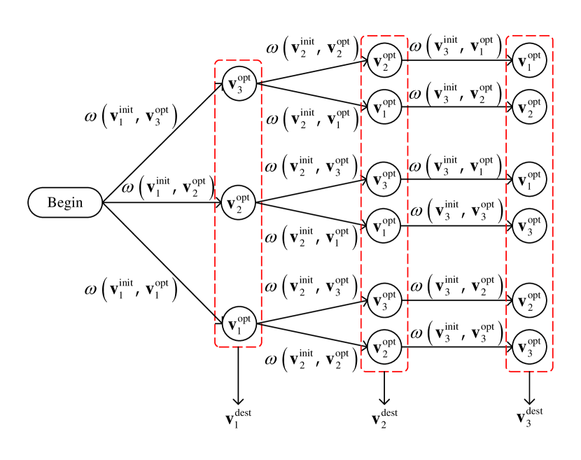
Figure 2: An example of APM with $\widetilde{N}=3$.

Define the initial and optimized antenna positions of $\widetilde{N}$ MAs before and after antenna position optimization as $\mathbf{v}_{\tilde{n}}^{\mathrm{init}}\in\mathbb{R}^{3\times 1}$ and $\mathbf{v}_{\tilde{n}}^{\mathrm{opt}}\in\mathbb{R}^{3\times 1}$ ($1\leq\tilde{n}\leq\widetilde{N}$), respectively. Prior works on MA-aided systems have yet incorporated the MA movement distance into the objective function or constraints of the optimization problem, apart from an initial investigation given in [40]. In other words, when moving MA $\tilde{n}$ from $\mathbf{v}_{\tilde{n}}^{\mathrm{init}}$ to $\mathbf{v}_{\tilde{n}}^{\mathrm{opt}}$, they do not consider the additional costs incurred by antenna movement in practical applications. The optimized position $\mathbf{v}_{\tilde{n}}^{\mathrm{opt}}$ may be far from the corresponding initial position $\mathbf{v}_{\tilde{n}}^{\mathrm{init}}$ but closer to another initial MA position. Furthermore, this oversight is especially significant in near-field ISAC scenarios because the large-size moving regions are deployed to fully enhance the system performance. As such, we propose an APM algorithm based on the greedy strategy to tackle this issue.

The total MA movement distance minimization problem is a shortest path search problem in tree graph. Fig. 2 shows an example for the case when $\widetilde{N}=3$, where

$$\omega\left({\mathbf{v}_{\tilde{n}}^{\mathrm{init}},\mathbf{v}_{\hat{n}}^{\mathrm{opt}}}\right)={\left\|{\mathbf{v}_{\tilde{n}}^{\mathrm{init}}-\mathbf{v}_{\hat{n}}^{\mathrm{opt}}}\right\|_{2}},\quad 1\leq{\hat{n}}\leq\widetilde{N},$$ (42)

is the path weight determined by the movement distance from $\mathbf{v}_{\tilde{n}}^{\mathrm{init}}$ to $\mathbf{v}_{\hat{n}}^{\mathrm{opt}}$. For each MA, the destination position, $\mathbf{v}_{\tilde{n}}^{\mathrm{dest}}\in\mathbb{R}^{3\times 1}$, can be selected according to path weights. Once a specific optimized position is selected by one MA, it becomes unavailable for the remaining MAs. Consequently, there are $\widetilde{N}!$ APM solutions.

To find the optimal APM solution that minimizes the total MA movement distance, a straightforward approach is to perform an exhaustive search over the $\widetilde{N}!$ solutions. However, this clearly results in high computational complexity, especially when $\widetilde{N}$ is large. As a result, we adopt the greedy strategy to identify a suboptimal solution. First, we initialize the antenna index set as $\widetilde{\mathcal{N}}^{0}=\left\{{1,\ldots,\widetilde{N}}\right\}$. Next, we sequentially select destination position $\mathbf{v}_{\tilde{n}}^{\mathrm{dest}}$ for each MA. Specifically, for MA $\tilde{n}$, we select the optimized position in updated antenna index set $\widetilde{\mathcal{N}}^{\tilde{n}-1}$ with the smallest path weight as its destination position, i.e.,

$$\mathbf{v}_{\tilde{n}}^{\mathrm{dest}}=\mathop{\arg\min}\limits_{\mathbf{v}_{\hat{n}}^{\mathrm{opt}}}\left\{{\omega\left({\mathbf{v}_{\tilde{n}}^{\mathrm{init}},\mathbf{v}_{\hat{n}}^{\mathrm{opt}}}\right)\left|{{\hat{n}}\in{{\widetilde{\mathcal{N}}}^{\tilde{n}-1}}}\right.}\right\}.$$ (43)

Then, we update the antenna index set by removing the index of the selected antenna position, i.e.,

$${\widetilde{\mathcal{N}}}^{\tilde{n}}={\widetilde{\mathcal{N}}}^{\tilde{n}-1}\backslash{\hat{n}}.$$ (44)

After the destination positions for all $\widetilde{N}$ MAs have been selected, the APM solution $\mathbf{v}_{\tilde{n}}^{\mathrm{dest}}$ for $1\leq\tilde{n}\leq\widetilde{N}$ is obtained.

Algorithm 4 APM algorithm for minimizing the total MA movement distance

0: $M$, $N$, $\mathbf{t}^{\mathrm{init}}$, $\mathbf{r}^{\mathrm{init}}$, $\mathbf{t}^{\mathrm{opt}}$, and $\mathbf{r}^{\mathrm{opt}}$.

0: $\mathbf{t}^{\mathrm{dest}}$ and $\mathbf{r}^{\mathrm{dest}}$.

1: Initialize the index sets of the transmit and receive MAs as $\mathcal{N}^{0}=\left\{{1,\ldots,N}\right\}$ and $\mathcal{M}^{0}=\left\{{1,\ldots,M}\right\}$, respectively;

2: for $n=1:1:N$ do

3:  Calculate path weight $\omega\left({\mathbf{t}_{n}^{\mathrm{init}},\mathbf{t}_{\hat{n}}^{\mathrm{opt}}}\right)$ according to (42);

4:  Select optimized position $\mathbf{t}_{\hat{n}}^{\mathrm{opt}}$ as transmit MA $n$’s destination position $\mathbf{t}_{n}^{\mathrm{dest}}$ according to (43);

5:  Update antenna index set $\mathcal{N}^{n}$ according to (44);

6: end for

7: for $m=1:1:M$ do

8:  Calculate path weight $\omega\left({\mathbf{r}_{m}^{\mathrm{init}},\mathbf{r}_{\hat{m}}^{\mathrm{opt}}}\right)$ according to (42);

9:  Select the optimized position $\mathbf{r}_{\hat{m}}^{\mathrm{opt}}$ as receive MA $m$’s destination position $\mathbf{r}_{m}^{\mathrm{dest}}$ according to (43);

10:  Update antenna index set $\mathcal{M}^{m}$ according to (44);

11: end for

12: return  $\mathbf{t}^{\mathrm{dest}}$ and $\mathbf{r}^{\mathrm{dest}}$.

Note that the aforementioned APM algorithm can be widely applied in MA-aided communication systems. For the proposed system, we need to perform APM separately for the transmit and receive MAs. In other words, we have $\widetilde{N}=N$ or $M$, $\mathbf{v}_{\tilde{n}}^{\mathrm{init}}=\mathbf{t}_{n}^{\mathrm{init}}$ or $\mathbf{r}_{m}^{\mathrm{init}}$, and $\mathbf{v}_{\tilde{n}}^{\mathrm{opt}}=\mathbf{t}_{n}^{\mathrm{opt}}$ or $\mathbf{r}_{m}^{\mathrm{opt}}$, where $\mathbf{t}_{n}^{\mathrm{init}}/\mathbf{r}_{m}^{\mathrm{init}}$ is the initial transmit/receive MA position and $\mathbf{t}_{n}^{\mathrm{opt}}/\mathbf{r}_{m}^{\mathrm{opt}}$ is the optimized transmit/receive MA position output by Algorithm 3. The corresponding processing steps are summarized in Algorithm 4. After that, the destination positions of transmit and receive MAs, $\mathbf{t}_{n}^{\mathrm{dest}}$ and $\mathbf{r}_{m}^{\mathrm{dest}}$ can be obtained.

III-D Overall Algorithm

Algorithm 5 Overall algorithm for solving problem (16) and minimizing total MA movement distance

0: $M$, $N$, $K$, $J$, $L$, $P^{\max}_{\mathrm{D}}$, $P^{\max}_{\mathrm{U}}$, $D$, $\Gamma$, $\mathcal{C}_{\mathrm{t}}$, $\mathcal{C}_{\mathrm{r}}$, $\rho_{\mathrm{SI}}$, $\lambda$, $\left\{{{\rho_{{\mathrm{D}_{k}}}}}\right\}$, $\left\{{{\rho_{{\mathrm{U}_{j}}}}}\right\}$, $\left\{{{\rho_{{\mathrm{S}_{l}}}}}\right\}$, $\left\{{{\mathbf{q}_{{\mathrm{U}_{j}}}}}\right\}$, $\left\{{{\mathbf{q}_{{\mathrm{D}_{k}}}}}\right\}$, $\left\{{{\mathbf{q}_{{\mathrm{S}_{l}}}}}\right\}$, $\mathbf{t}^{\mathrm{init}}$, and $\mathbf{r}^{\mathrm{init}}$.

0: $\mathbf{u}_{l}$, $\mathbf{b}_{j}$, $\mathbf{S}_{l}$, $\mathbf{w}_{k}$, $p_{j}$, $\mathbf{t}^{\mathrm{dest}}$, and $\mathbf{r}^{\mathrm{dest}}$.

1: Solving problem (16) by Algorithm 3 to obtain optimized $\mathbf{u}_{l}$, $\mathbf{b}_{j}$, $\mathbf{S}_{l}$, $\mathbf{w}_{k}$, $p_{j}$, $\mathbf{t}^{\mathrm{opt}}$, and $\mathbf{r}^{\mathrm{opt}}$;

2: Search destination positions for transmit and receive MAs, $\mathbf{t}^{\mathrm{dest}}$ and $\mathbf{r}^{\mathrm{dest}}$, by Algorithm 4;

3: return  $\mathbf{u}_{l}$, $\mathbf{b}_{j}$, $\mathbf{S}_{l}$, $\mathbf{w}_{k}$, $p_{j}$, $\mathbf{t}^{\mathrm{dest}}$, and $\mathbf{r}^{\mathrm{dest}}$.

The detailed overall algorithm for solving problem (16) and minimizing the total MA movement distance is summarized in Algorithm 5. Specifically, the optimized transmit beamformers, $\mathbf{w}_{k}$, sensing signal covariance matrices, $\mathbf{S}_{l}$, receive beamformers, $\mathbf{u}_{l}$ and $\mathbf{b}_{j}$, UL power allocation, $p_{j}$, and MA positions, $\mathbf{t}^{\mathrm{opt}}$ and $\mathbf{r}^{\mathrm{opt}}$, are obtained by Algorithm 3 (Line 1). Subsequently, the destination positions of transmit and receive MAs, $\mathbf{t}^{\mathrm{dest}}$ and $\mathbf{r}^{\mathrm{dest}}$, are searched by Algorithm 4 to minimize the total MA movement distance (Line 2).

III-E Convergence and Complexity Analysis

As the RP algorithm only executes the selection of candidate MA positions, its convergence depends on Algorithm 2. The convergence of Algorithm 2 is guaranteed by the following inequality:

$$WSR\left(\mathbf{u}_{l}^{\tilde{c}},\mathbf{b}_{j}^{\tilde{c}},\mathbf{S}_{l}^{\tilde{c}},\mathbf{w}_{k}^{\tilde{c}},p_{j}^{\tilde{c}}\right)$$

$$\mathop{\geq}\limits^{\left({{\alpha_{1}}}\right)}WSR\left(\mathbf{u}_{l}^{\tilde{c}},\mathbf{b}_{j}^{\tilde{c}},\mathbf{S}_{l}^{\tilde{c}-1},\mathbf{w}_{k}^{\tilde{c}-1},p_{j}^{\tilde{c}-1}\right)$$

$$\mathop{\geq}\limits^{\left({{\alpha_{2}}}\right)}WSR\left(\mathbf{u}_{l}^{\tilde{c}-1},\mathbf{b}_{j}^{\tilde{c}-1},\mathbf{S}_{l}^{\tilde{c}-1},\mathbf{w}_{k}^{\tilde{c}-1},p_{j}^{\tilde{c}-1}\right),$$ (45)

where inequality ${\left({{\alpha_{1}}}\right)}$ holds because $\left\{\mathbf{S}_{l}^{\tilde{c}},\mathbf{w}_{k}^{\tilde{c}},p_{j}^{\tilde{c}}\right\}$ are the optimized sensing signal covariance matrices, transmit beamformers, and UL power allocation via Algorithm 1 under the current $\left\{\mathbf{u}_{l}^{\tilde{c}},\mathbf{b}_{j}^{\tilde{c}}\right\}$, and inequality ${\left({{\alpha_{2}}}\right)}$ holds because $\left\{\mathbf{u}_{l}^{\tilde{c}},\mathbf{b}_{j}^{\tilde{c}}\right\}$ are the optimal receive beamformers for maximizing SINRs (12) and (13) under the current $\left\{\mathbf{S}_{l}^{\tilde{c}-1},\mathbf{w}_{k}^{\tilde{c}-1},p_{j}^{\tilde{c}-1}\right\}$. Thus, the objective value is non-decreasing during the iterations in Algorithm 2. Meanwhile, the objective value is upper-bounded due to finite communication resources. As such, the convergence of Algorithm 2 is guaranteed. Moreover, the convergence is verified by the simulations in Section IV-B.

The main computational complexity of the overall algorithm, i.e., Algorithm 5, is caused by the iterations of Algorithm 2, the selections of Algorithm 3, and the searches of Algorithm 4. In Algorithm 2, the computational complexity for calculating receive beamformers is $\mathcal{O}\left(\left(L+J\right)M^{3}\right)$ due to the matrix inversion in (20) and (21). The computational complexity of Algorithm 1 for optimizing transmit beamformers, sensing signal covariance matrices, and UL power allocation is $\mathcal{O}\left(C_{\mathrm{SCA}}\left(\left(L+K\right)N^{3.5}+J^{3.5}\right)\right)$ due to solving the SDR problem iteratively, where $C_{\mathrm{SCA}}$ is the number of iterations for SCA. Therefore, the computational complexity of Algorithm 2 is $o_{1}=\mathcal{O}\left(\widetilde{C}_{\mathrm{AO}}\left(\left(L+J\right)M^{3}+C_{\mathrm{SCA}}\left(\left(L+K\right)N^{3.5}+J^{3.5}\right)\right)\right)$, where $\widetilde{C}_{\mathrm{AO}}$ is the number of iterations for AO. In addition, the computational complexity of Algorithm 4 for matching antenna positions is $o_{2}=\mathcal{O}\left({\frac{1}{2}\left({N\left({N+1}\right)+M\left({M+1}\right)}\right)}\right)$. As a result, with the number of candidate MA position pairs $\Gamma$, the computational complexity of the overall algorithm is $\mathcal{O}\left(\Gamma o_{1}+o_{2}\right)$.

IV Performance Evaluation

In this section, we provide the simulation results to evaluate the performance of the proposed MA-aided near-field ISAC system. First, the simulation setup is introduced, and then the numerical results are presented.

IV-A Simulation Setup

TABLE I: Simulation Parameters

Parameter	Description	Value
$A_{\mathrm{t}}$, $A_{\mathrm{r}}$	Side length of moving region	$100\lambda\times 100\lambda$
$N$, $M$	Number of MAs	8
$L$, $J$, $K$	Number of targets/users	2
$C$, $\widetilde{C}$	Maximum number of iterations	100
$\Gamma$	Number of MA position pairs	100
$\epsilon$, $\tilde{\epsilon}$	Error tolerance	$10^{-3}$
$\rho_{\mathrm{SI}}$	SI loss coefficient	-100 dB
$\rho_{\mathrm{S}_{l}}$	Round-trip channel coefficient	-50 dB
$P_{\mathrm{U}}^{\mathrm{max}}$	Maximum UL transmit power	10 dBm
$P_{\mathrm{D}}^{\mathrm{max}}$	Maximum DL transmit power	40 dBm
$D$	Minimum inter-MA distance	$\lambda/2$
$\sigma^{2}_{\mathrm{BS}}$, $\sigma^{2}_{k}$	Average noise power	-70 dBm

In the simulation, the sensing targets and users are randomly distributed within a semicircular region on the ground centered at the BS, with horizontal distances from the BS to the targets/users ranging from 25 to 30 meters (m). The transmit and receive MA arrays are mounted on a full-duplex BS at a height of 15 m in a horizontal arrangement. The transmit and receive regions for the MA movement are square regions with side lengths of $A_{\mathrm{t}}$ and $A_{\mathrm{r}}$, respectively. The carrier frequency is set as 30 GHz ($\lambda=0.01$ m). The pass loss coefficients $\rho_{{\mathrm{D}_{k}}}$ and $\rho_{{\mathrm{U}_{j}}}$ are determined by the uniform spherical wave (USW) model [35, Equation (35)]. Without loss of generality, we assume that the transmit and receive regions have equal side lengths, i.e., $A_{\mathrm{t}}=A_{\mathrm{r}}$, the numbers of transmit and receive MAs are equal, i.e., $N=M$, and the rate weights are equal, i.e., ${\varpi_{{\mathrm{S}_{l}}}}={\varpi_{{\mathrm{U}_{j}}}}={\varpi_{{\mathrm{D}_{k}}}}=\frac{1}{L+J+K}$. Unless otherwise specified, the default simulation parameters are listed in Table I.

IV-B Convergence Evaluation of Algorithm 2

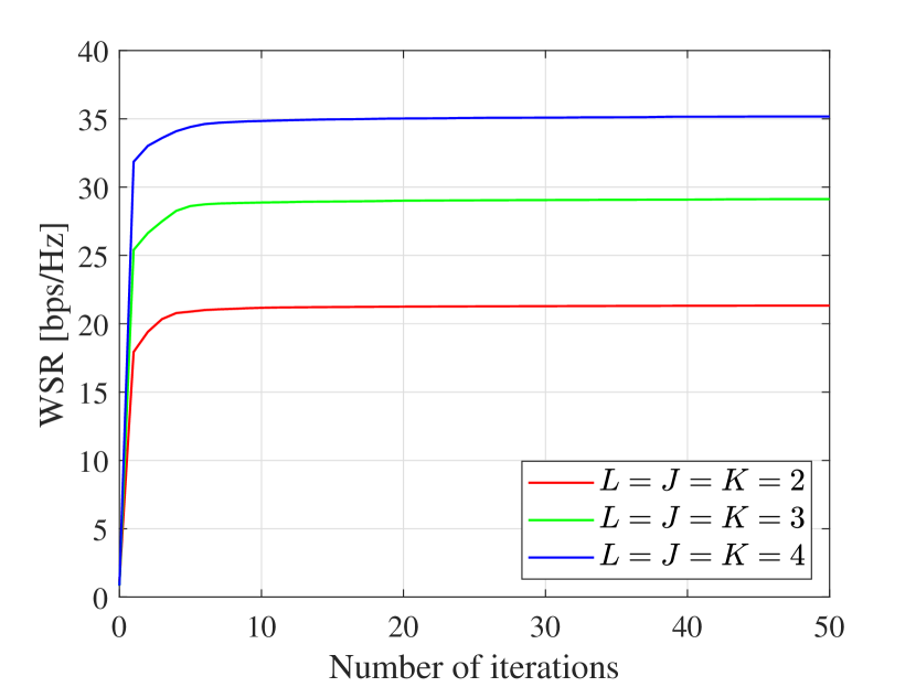
Figure 3: Convergence evaluation of Algorithm 2.

We first evaluate in Fig. 3 the convergence performance of the proposed Algorithm 2, under different numbers of targets/users. As can be observed, the algorithm demonstrates rapid convergence in all scenarios, with the objective value stabilizing within 10 iterations. This confirms the previous discussion regarding the convergence of Algorithm 2 in Section III-E. Moreover, the WSR improves as the number of targets/users increases, since the additional targets/users can leverage the redundant spatial DoFs to further enhance the overall system performance.

IV-C Beamfocusing in MA-Aided Near-Field ISAC

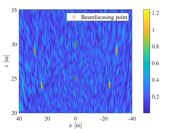
(a) $A_{\mathrm{t}}=100\lambda$

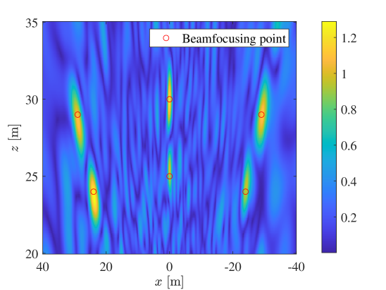
(b) $A_{\mathrm{t}}=30\lambda$

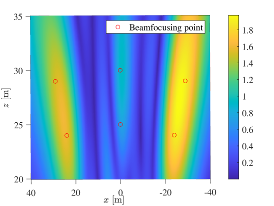
(c) $A_{\mathrm{t}}=5\lambda$

Figure 4: Beampattern under different sizes of the moving region.

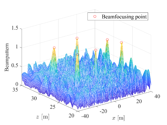
(a) [25, 30] m

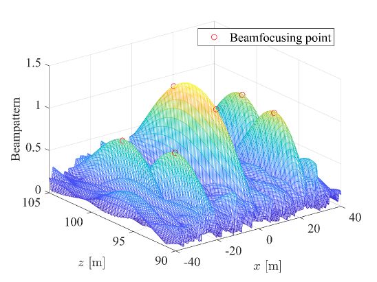
(b) [95, 100] m

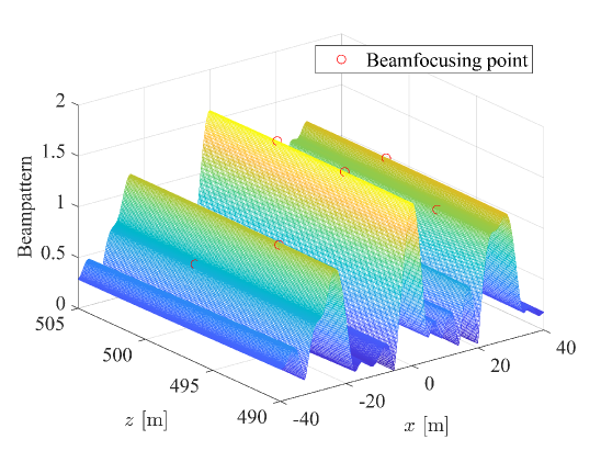
(c) [495, 500] m

Figure 5: Beampattern under different distances between the BS and beamfocusing points.

To intuitively demonstrate the advantages of large-size moving regions in near-field ISAC systems, we present the beampattern corresponding to the optimized geometry of the transmit MA array with $N=128$ in Figs. 4 and 5. The beampattern for the receive MA array can be similarly obtained and is thus omitted here for brevity. Specifically, we calculate the array response vector

$$\mathbf{a}\left(\mathbf{q}\right)={\left[{{e^{\mathrm{j}\frac{{2\pi}}{\lambda}{{\left\|{{\mathbf{t}_{1}}-\mathbf{q}}\right\|}_{2}}}},\ldots,{e^{\mathrm{j}\frac{{2\pi}}{\lambda}{{\left\|{{\mathbf{t}_{N}}-\mathbf{q}}\right\|}_{2}}}}}\right]^{T}}\in{\mathbb{C}^{N\times 1}},$$ (46)

for all positions $\mathbf{q}$ within a defined rectangular region on the ground. Then, the beamfocusing at $B$ locations, i.e., ${\tilde{\mathbf{q}}}_{b}\in{\mathbb{R}^{3\times 1}}$, $b\in\mathcal{B}=\left\{1,\ldots,B\right\}$, is achieved by setting the beamforming vector as the sum of the array response vectors at these beamfocusing points, i.e.,

$${\mathbf{w}_{\mathrm{bf}}} =\sum\limits_{b\in\mathcal{B}}{\mathbf{a}\left({{{\tilde{\mathbf{q}}}_{b}}}\right)}$$

$$=\sum\limits_{b\in\mathcal{B}}{{{\left[{{e^{\mathrm{j}\frac{{2\pi}}{\lambda}{{\left\|{{\mathbf{t}_{1}}-{{\tilde{\mathbf{q}}}_{b}}}\right\|}_{2}}}},\ldots,{e^{\mathrm{j}\frac{{2\pi}}{\lambda}{{\left\|{{\mathbf{t}_{N}}-{{\tilde{\mathbf{q}}}_{b}}}\right\|}_{2}}}}}\right]}^{T}}}\in{\mathbb{C}^{N\times 1}},$$ (47)

Therefore, the beamforming gain at position $\mathbf{q}$ can be calculated as

$$G\left(\mathbf{q}\right)=\frac{1}{N}\left|{\mathbf{w}_{\mathrm{bf}}^{H}\mathbf{a}\left(\mathbf{q}\right)}\right|.$$ (48)

As shown in Fig. 4, when $A_{\mathrm{t}}=100\lambda$ (see Fig. 4LABEL:sub@bp_dis1), the beam is precisely focused at the multiple desired locations, and the main lobes of the beam are extremely narrow. This indicates that the beam focused on the desired locations causes minimal interference leakage to other locations, allowing the near-field ISAC system to achieve excellent performance in multi-target sensing and multi-user communication through joint resolutions in both the distance and angle domains. As the size of the moving region decreases ((see Figs. 4LABEL:sub@bp_dis2 and 4LABEL:sub@bp_dis3), the beam’s main lobes become wider due to the reduced maximum aperture achievable by the MA array. This results in significant interference to targets/users at undesired locations, thereby degrading the overall system performance. Notably, when $A_{\mathrm{t}}=5\lambda$, the beamfocusing points are already in the far-field region, resulting in a loss of resolution in the distance domain and retaining only angular discrimination. In other words, when multiple targets and users are located in the same direction relative to the BS, the far-field ISAC system cannot provide effective sensing and communication services for them.

In addition, Fig. 5 provides a 3D perspective on the variations in beampatterns across different distance intervals between the BS and beamfocusing points. The beamforming gains in Fig. 5LABEL:sub@bp_dis1 at the beamfocusing points are significantly higher compared to the other locations. As the distance between the BS and beamfocusing points increases, the interference leakage from the beam’s main lobes to locations that are not beamfocusing points becomes more pronounced because the spherical wave approximates more closely to the plane wave, leading to a gradual disappearance of near-field beamfocusing characteristics. The beamforming gains in Fig. 5LABEL:sub@bp_dis3 are nearly uniform in the same direction, which makes it impossible to distinguish between different beamfocusing points along that direction.

Overall, the additional distance dimension of near-field ISAC, compared to far-field ISAC, allows for beamfocusing that enhances the performance of multi-target sensing and multi-user communication. The MA system, which has a larger aperture size of the antenna array compared to conventional FPA systems, naturally expands the near-field region. As a result, the MA-aided near-field ISAC system can benefit from the enlarged near-field region achieved by the large moving region.

IV-D Performance Comparison with Benchmark Schemes

To gain more insight, we compare the performance of the proposed scheme (labeled as MA) with benchmark schemes. The considered benchmark schemes for setting antennas’ positions are listed as follows: 1) FPA with full aperture (FPAF): The antenna’s positions, $\mathbf{t}$ and $\mathbf{r}$, are set according to the transmit and receive uniform planar arrays (UPAs) with the largest achievable apertures, $A_{\mathrm{t}}\times A_{\mathrm{t}}$ and $A_{\mathrm{r}}\times A_{\mathrm{r}}$, respectively; and 2) FPA with half-wavelength antenna spacing (FPAH): The antenna’s positions, $\mathbf{t}$ and $\mathbf{r}$, are set according to the transmit and receive UPAs with half-wavelength inter-antenna spacing both horizontally and vertically.

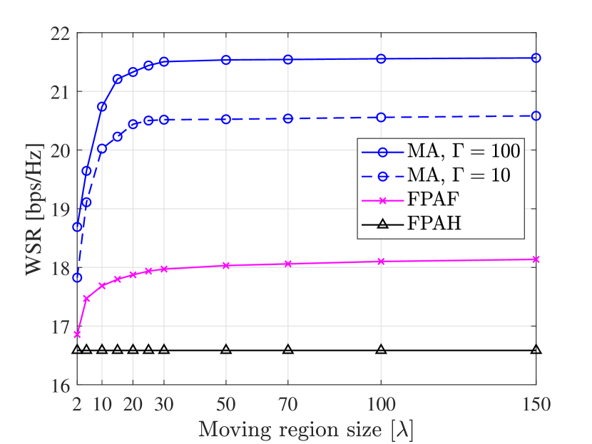
Figure 6: Comparison of WSR between the proposed and benchmark schemes w.r.t. the moving region size.

Fig. 6 compares the WSRs of different schemes versus the moving region size. As can be seen, the WSRs of the MA and FPAF schemes continuously increase when the moving region size is less than $30\lambda$, and stabilize when the size exceeds $30\lambda$. This is because the increase in the moving region size provides two advantages: 1) expand the optimization space for the antenna position optimization; and 2) enlarge the equivalent array aperture, thereby extending the near-field region, within which the resolution for multiple locations can be achieved. The MA scheme fully leverages both advantages to improve system performance. The FPAF scheme benefits only from advantage 2). The FPAH scheme fails to capitalize on either of these two advantages. As a result, the MA scheme achieves a 13.57% or 19.07% WSR gain over the FPAF scheme when $\Gamma=10$ or $\Gamma=100$, respectively. The WSR of the FPAH scheme, however, remains unchanged because of the fixed antennas’ positions and array aperture. Furthermore, for the MA scheme, $\Gamma=100$ achieves better system performance than $\Gamma=10$ due to the availability of more candidate MA positions, at the cost of increased computational complexity.

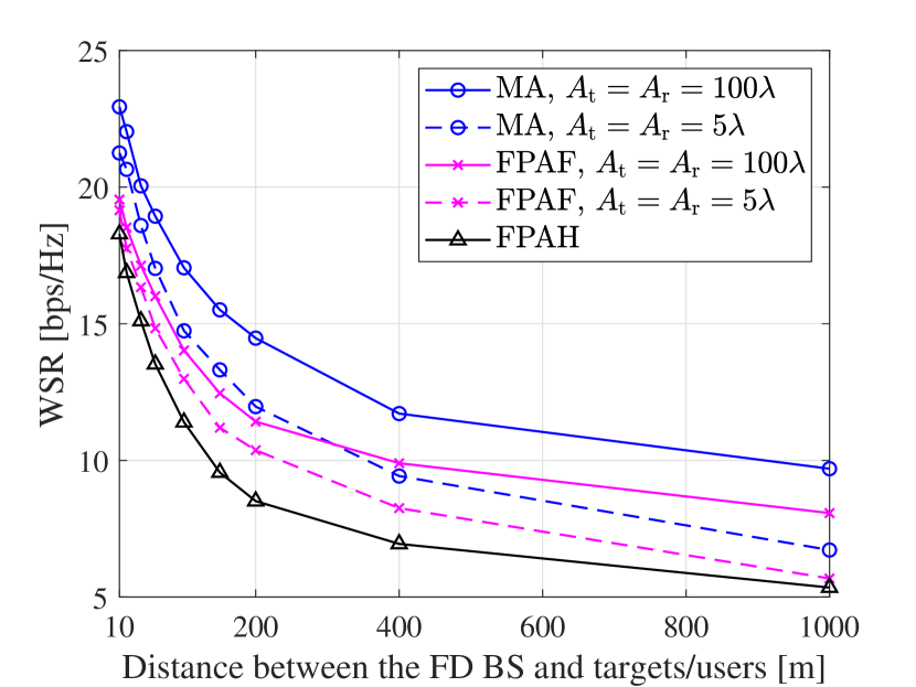
Figure 7: Comparison of WSR between the proposed and benchmark schemes w.r.t. the distance between the BS and targets/users.

In Fig. 7, we compare the WSRs of the proposed and benchmark schemes w.r.t. the distance between the BS and targets/users. The distances between the BS and different targets/users are set within a 5-meter interval, centered around a specified distance. We can see that as the distance increases, the WSR of all schemes decreases. This is because the increase in distance weakens system performance in the following two aspects: 1) increased path loss; and 2) the transition from near-field ISAC to far-field ISAC, which leads to the gradual loss of the distance dimension in the ISAC system. However, in the same communication scenario, the MA scheme still outperforms the FPAF or FPAH scheme due to the additional DoFs introduced by antenna position optimization.

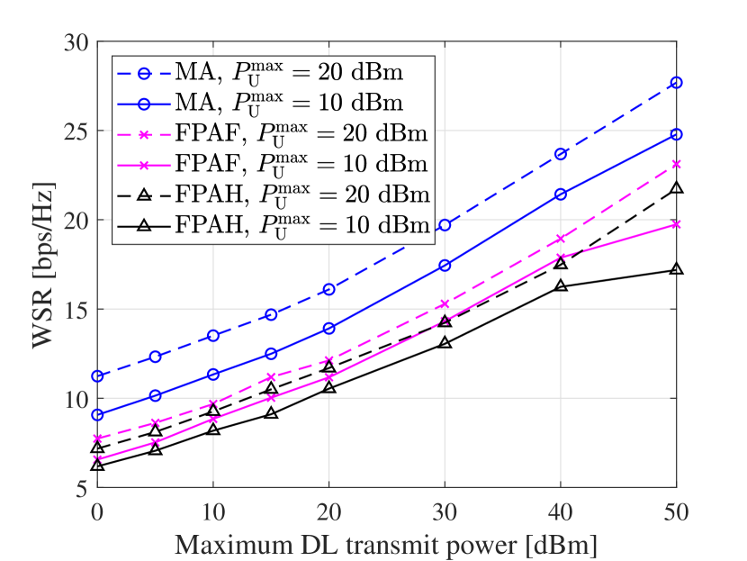
Figure 8: Comparison of WSR between the proposed and benchmark schemes w.r.t. the maximum DL transmit power.

Next, we show the WSRs of the proposed and benchmark schemes w.r.t. the maximum DL transmit power under different maximum UL transmit power constraints in Fig. 8. Overall, the WSRs of all schemes improve as the maximum DL transmit power increases, since higher DL transmit power ensures more reliable DL transmission quality. However, the high DL transmit power can cause strong echo signals from the sensing targets and SI, which in turn degrade the SINRs of the UL users. Therefore, as shown in Fig. 8, when $P^{\mathrm{max}}_{\mathrm{D}}\geq 40$ dBm, both the FPAF and FPAH schemes exhibit a noticeable slowdown in WSR increase compared to the MA scheme at low maximum UL transmit power case, i.e., $P^{\mathrm{max}}_{\mathrm{U}}=10$ dBm. In addition, compared to FPA-based schemes, the MA scheme can save DL transmit power at the same WSR level by leveraging antenna movement to effectively reconfigure the channels.

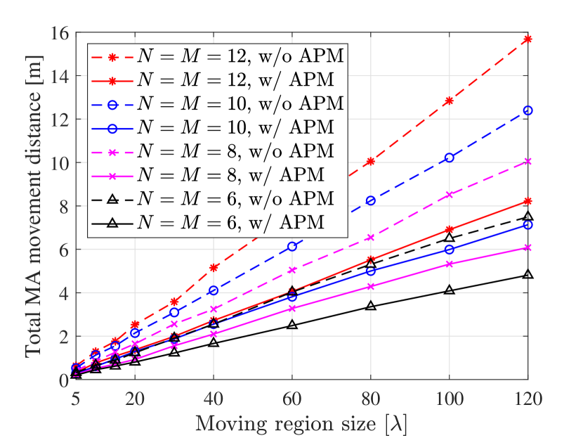
Figure 9: Total MA movement distance for schemes with (w/) or without (w/o) APM algorithm w.r.t. the moving region size.

Finally, Fig. 9 illustrates the total MA movement distance for schemes with (w/) or without (w/o) APM algorithm w.r.t. the moving region size under different numbers of MAs. It can be seen that the total MA movement distance increases linearly with the size of the moving region, and the APM algorithm significantly reduces this distance. Moreover, as the number of MAs increases, the gap between the schemes w/ and w/o APM algorithm widens. Specifically, when the moving region size is $120\lambda$, the proposed APM algorithm reduces the total MA movement distance by 35.79%, 39.50%, 42.46%, and 47.59% for $N=M=$ 6, 8, 10, and 12, respectively. Typically, in MA-aided near-field ISAC systems, the size of moving region and the number of MAs are large. Therefore, solely considering antenna position optimization without accounting for APM leads to long MA movement distance, thereby increasing the time delay and hardware burden.

V Conclusion

In this paper, we investigated the MA-aided near-field ISAC system. We characterized the near-field sensing and communication channels w.r.t. MA positions using the spherical wave model and formulated a joint optimization problem to maximize the system’s WSR achievable for both communications and sensing. To solve this non-convex optimization problem, we proposed a two-layer RP algorithm where multiple MA positions were randomly initialized. For each MA position, the beamformers, sensing signal covariance matrices, and UL power allocation were iteratively optimized using the AO algorithm until convergence. The MA position that achieves the maximum WSR was then selected as the optimized position. Moreover, considering the large size of moving region and the large number of antennas in near-field MA systems, we proposed an APM algorithm based on the greedy strategy to reduce the total MA movement distance, thereby alleviating the cost of antenna movement. Simulation results verified the effectiveness of the proposed algorithms and the advantages of the considered MA-aided ISAC scheme compared to conventional FPA-based schemes. Furthermore, the results showed that equipping the BS with large regions for free MA movement increases the equivalent array aperture, thereby significantly expanding the near-field region without requiring more antennas or higher frequencies. Compared to the far-field ISAC system, the additional distance dimension introduced by the near-field ISAC system can enhance system performance for multi-target sensing and multi-user communication through precise beamfocusing. This can be more efficiently exploited by optimally designing the MAs’ positions matching the ISAC channels.

References

- [1] Y. Zhuo, T. Mao, H. Li, C. Sun, Z. Wang, and Z. Han, “Multi-beam integrated sensing and communication: State-of-the-art, challenges and opportunities,” IEEE Commun. Mag., vol. 62, no. 9, pp. 90-96, Sep. 2024.
- [2] X. Shao, C. You, W. Ma, X. Chen, and R. Zhang, “Target sensing with intelligent reflecting surface: Architecture and performance,” IEEE J. Sel. Areas Commun., vol. 40, no. 7, pp. 2070-2084, Jul. 2022.
- [3] Y. Gong, X. Li, F. Meng, L. Liu, M. Guizani, and Z. Xu, “Toward green RF chain design for integrated sensing and communications: Technologies and future directions,” IEEE Commun. Mag., vol. 62, no. 9, pp. 36-42, Sep. 2024.
- [4] F. Liu, Y. Cui, C. Masouros, J. Xu, T. X. Han, Y. C. Eldar, and S. Buzzi, “Integrated sensing and communications: Toward dual-functional wireless networks for 6G and beyond,” IEEE J. Sel. Areas Commun., vol. 40, no. 6, pp. 1728-1767, Jun. 2022.
- [5] X. Chen, X, He, Z, Feng, Z, Wei, Q, Zhang, and X. Yuan, “Joint localization and communication enhancement in uplink integrated sensing and communications system with clock asynchronism,” IEEE J. Sel. Areas Commun., vol. 42, no. 10, pp. 2659-2673, Oct. 2024.
- [6] J. Dai, C. Liu, C. Pan, and K. Wang, “Secure downlink transmission for integrated sensing, energy, and communication systems,” IEEE Commun. Lett., vol. 28, no. 9, pp. 1996-2000, Sep. 2024.
- [7] X. Wang, Z. Fei, J. A. Zhang, and J. Huang, “Sensing-assisted secure uplink communications with full-duplex base station,” IEEE Commun. Lett., vol. 26, no. 2, pp. 249-253, Feb. 2022.
- [8] C. G. Tsinos, A. Arora, S. Chatzinotas, and B. Ottersten, “Joint transmit waveform and receive filter design for dual-function radar-communication systems,” IEEE J. Sel. Topics Signal Process., vol. 15,no. 6, pp. 1378–1392, Nov. 2021.
- [9] C.-Y. Chen and P. P. Vaidyanathan, “MIMO radar waveform optimization with prior information of the extended target and clutter,” IEEE Trans. Signal Process., vol. 57, no. 9, pp. 3533–3544, Sep. 2009.
- [10] L. Wu, P. Babu, and D. P. Palomar, “Transmit waveform/receive filter design for MIMO radar with multiple waveform constraints,” IEEE Trans. Signal Process., vol. 66, no. 6, pp. 1526–1540, Mar. 2018.
- [11] D. Galappaththige, C. Tellambura, and A. Maaref, “Integrated sensing and backscatter communication,” IEEE Wireless Commun. Lett., vol. 12, no. 12, pp. 2043-2047, Dec. 2023.
- [12] J. A. Zhang et al., “Enabling joint communication and radar sensing in mobile networks-A survey,” IEEE Commun. Surveys Tuts., vol. 24, no. 1, pp. 306-345, 1st Quart., 2022.
- [13] B. He, F. Wang, and J. Cheng, “Joint secure transceiver design for integrated sensing and communication,” IEEE Trans. Wireless Commun., vol. 23, no. 10, pp. 13377-13393, Oct. 2024.
- [14] Z. He, W. Xu, H. Shen, D. W. K. Ng, Y. C. Eldar, and X. You, “Full-duplex communication for ISAC: Joint beamforming and power optimization,” IEEE J. Sel. Areas Commun., vol. 41, no. 9, pp. 2920-2936, Sep. 2023.
- [15] Z. Wang, X. Mu, and Y. Liu, “Bidirectional integrated sensing and communication: Full-duplex or half-duplex?,” IEEE Trans. Wireless Commun., vol. 23, no. 8, pp. 8184-8199, Aug. 2024.
- [16] W. Lyu, S. Yang, Z. Zhang, C. Assi, C. Yuen, “Movable antenna enabled integrated sensing and communication,” 2024, arXiv:2410.19763.
- [17] W. Ma, L. Zhu, and R. Zhang, “MIMO capacity characterization for movable antenna systems,” IEEE Trans. Wireless Commun., vol. 23, no. 4, pp. 3392-3407, Apr. 2024.
- [18] L. Zhu, W. Ma, and R. Zhang, “Movable antennas for wireless communication: Opportunities and challenges,” IEEE Commun. Mag., vol. 62, no. 6, pp. 114-120, Jun. 2024.
- [19] X. Shao, Q. Jiang, and R. Zhang, “6D movable antenna based on user distribution: Modeling and optimization,” IEEE Trans. Wireless Commun., Nov. 13, 2024, early access, doi: 10.1109/TWC.2024.3492195.
- [20] X. Shao, R. Zhang, Q. Jiang, and R. Schober, “6D movable antenna enhanced wireless network via discrete position and rotation optimization,” 2024, arXiv:2403.17122.
- [21] X. Shao and R. Zhang, “6DMA enhanced wireless network with flexible antenna position and rotation: Opportunities and challenges,” 2024, arXiv:2406.06064.
- [22] X. Shao, R. Zhang, Q. Jiang, J. Park, T. Q. S. Quek, and R. Schober, “Distributed channel estimation and optimization for 6D movable antenna: Unveiling directional sparsity,” 2024, arXiv:2409.16510.
- [23] W. Ma, L. Zhu, and R. Zhang, “Movable antenna enhanced wireless sensing via antenna position optimization,” IEEE Trans. Wireless Commun., vol. 23, no. 11, pp. 16575-16589, Nov. 2024.
- [24] H. Qin, W. Chen, Q. Wu, Z. Zhang, Z. Li, and N. Cheng, “Cramér-Rao bound minimization for movable antenna-assisted multiuser integrated sensing and communications,” IEEE Wireless Commun. Lett., vol. 13, no. 12, pp. 3404-3408, Dec. 2024.
- [25] X. Shao, R. Zhang, and R. Schober, “Exploiting six-dimensional movable antenna for wireless sensing,” IEEE Wireless Commun. Lett., Oct. 29, 2024, early access, doi: 10.1109/LWC.2024.3487966.
- [26] J. Ding, Z. Zhou, W. Li, C. Wang, L. Lin, and B. Jiao, “Movable antenna-enabled co-frequency co-time full-duplex wireless communication,” IEEE Commun. Lett., vol. 28, no. 10, pp. 2412-2416, Oct. 2024.
- [27] J. Ding, Z. Zhou, C. Wang, W. Li, L. Lin, and B. Jiao, “Secure full-duplex communication via movable antennas,” 2024, arXiv:2403.20025.
- [28] J. Ding, Z. Zhou, and B. Jiao, “Movable antenna-aided secure full-duplex multi-user communications,” 2024, arXiv:2407.10393.
- [29] L. Lin, J. Ding, Z. Zhou, and B. Jiao, “Power-efficient full-duplex satellite communications aided by movable antennas,” IEEE Wireless Commun. Lett., Dec. 17, 2024, early access, doi: 10.1109/LWC.2024.3519367.
- [30] S. Peng, C. Zhang, Y. Xu, Q. Wu, X. Ou, and D. He, “Joint antenna position and beamforming optimization with self-interference mitigation in MA-ISAC system,” 2024, arXiv:2408.00413.
- [31] Z. Li, J. Ba, Z. Su, H. Peng, Y. Wang, W. Chen, and Q. Wu, “Joint discrete antenna positioning and beamforming optimization in movable antenna enabled full-duplex ISAC networks,” 2024, arXiv:2411.04419.
- [32] Y. Guo, W. Chen, Q. Wu, Y. Liu, Q. Wu, K. Wang, J. Li, and L. Xu, “Movable antenna enhanced networked full-duplex integrated sensing and communication system,” 2024, arXiv:2411.09426.
- [33] J. Ding, L. Zhu, Z. Zhou, B. Jiao, and R. Zhang, “Near-field multiuser communications aided by movable antennas,” IEEE Wireless Commun. Lett., Nov. 4, 2024, early access, doi: 10.1109/LWC.2024.3490697.
- [34] L. Zhu, W. Ma, Z. Xiao, and R. Zhang, “Movable antenna enabled near-field communications: Channel modeling and performance optimization,” 2024, arXiv:2409.19316.
- [35] Y. Liu, Z. Wang, J. Xu, C. Ouyang, X. Mu, and R. Schober, “Near-field communications: A tutorial review,” IEEE Open J. Commun. Soc., vol. 4,pp. 1999-2049, Aug. 2023.
- [36] Z. Wang, X. Mu, and Y. Liu, “Near-field integrated sensing and communications,” IEEE Commun. Lett., vol. 27, no. 8, pp. 2048-2052, Aug. 2023.
- [37] D. Galappaththige, S. Zargari, C. Tellambura, and G. Y. Li, “Near-field ISAC: Beamforming for multi-target detection,” IEEE Wireless Commun. Lett., vol. 13, no. 7, pp. 1938-1942, July 2024.
- [38] G. Hu et al., “Movable antennas-enabled two-user multicasting: Do we really need alternating optimization for minimum rate maximization?,” IEEE Trans. Veh. Technol, Nov. 18, 2024, early access, doi: 10.1109/TVT.2024.3500138.
- [39] D. Xu, X. Yu, Y. Sun, D. W. K. Ng, and R. Schober, “Resource allocation for IRS-assisted full-duplex cognitive radio systems,” IEEE Trans. Commun., vol. 68, no. 12, pp. 7376-7394, Dec. 2020.
- [40] Q. Li, W. Mei, B. Ning, and R. Zhang, “Minimizing movement delay for movable antennas via trajectory optimization,” 2024, arXiv:2408.12813.