RUP-24-22
STUPP-24-275
Oscillons in AdS space
Takaaki Ishii1***E-mail: ishiitkatrikkyo.ac.jp,
Takaki Matsumoto2,3†††E-mail: takaki-matsumotoatejs.seikei.ac.jp,
Kanta Nakano3‡‡‡E-mail: k.nakano.233atms.saitama-u.ac.jp,
Ryosuke Suda3§§§E-mail: r.suda.813atms.saitama-u.ac.jp
and Kentaroh Yoshida3¶¶¶E-mail: kenyoshidaatmail.saitama-u.ac.jp
1Department of Physics, Rikkyo University,
3-34-1 Nishi-Ikebukuro, Toshima-ku, Tokyo 171-8501, Japan
2Seikei University,
3-3-1 Kichijoji-Kitamachi, Musashino-shi, Tokyo 180-8633, Japan
3Graduate School of Science and Engineering, Saitama University,
255 Shimo-Okubo, Sakura-ku, Saitama 338-8570, Japan
Abstract
We study oscillons in a real scalar field theory in a (3+1)-dimensional AdS space with global coordinates. The initial configuration is given by a Gaussian shape with an appropriate core size as in Minkowski spacetime. The solution exhibits a long lifetime. In particular, since the AdS space can be seen as a box, the recurrence phenomenon can be observed under suitable conditions. Finally, we discuss some potential applications of the oscillon in the context of AdS/CFT duality.
1 Introduction
Oscillons are localized and long-lived excitations in a real scalar field theory with a self-interacting potential in dimensions (where is the number of spatial directions). It is well known that excitations in (1+1)-dimensional Minkowski spacetime may be stable due to Derrick’s theorem [1]. In higher dimensions (), there is no such theorem and the mechanism to stabilize excitations has been unknown. However, there may be localized and long-lived excitations, whose lifetime is extremely long but finite. They are oscillons.
The oscillons have some basic characteristics, which are summarized as follows. The oscillons are
-
1.
stabilized by non-linear effect from non-trivial potential,
-
2.
time-dependent, long-lived excitations with no topological charge,
-
3.
spherically symmetric,
-
4.
strongly sensitive to the initial configuration e.g., Gaussian profile.
The oscillons were originally recognized by Gleiser [2] and were theoretically grounded in a series of papers [3, 4, 5]. However, it is fair to say that the fundamental mechanism to ensure the longevity of oscillons has been quite unclear, although we know that some specific initial configurations lead to the long-lived excitations phenomenologically.
In this letter, we investigate oscillons in a real scalar field theory in a (3+1)-dimensional anti-de Sitter (AdS) space with global coordinates. If we take the Gaussian profile as the initial configuration, oscillons can be realized, just as in Minkowski spacetime. The oscillon behavior depends on the curvature radius . In particular, since the AdS space can be seen as a box, a phenomenon of recurrence can be observed for suitable values of . This may be worth noting because, although the system is non-integrable, the oscillons exhibit some integrable-ish properties.
This letter is organized as follows. In Section 2, we will introduce the setup to study oscillons in AdS. In Section 3, we perform numerical computations and show the existence of oscillons. In particular, the oscillons exhibit the recurrence phenomenon. Section 4 is devoted to the conclusion and discussion.
2 Setup
In this section, let us prepare the system we will analyze. We first introduce the classical action of a real scalar field theory with a self-interacting potential in a (+1)-dimensional AdS space. Then the initial and boundary conditions to realize oscillons will be introduced by following the Minkowski case [3]. Finally, the shell energy is defined so as to figure out the behavior of the oscillons and to track the radiations emitted from the shell.
2.1 A real scalar field theory in AdS
We consider a real scalar field theory in a dimensional global AdS space with the metric
| (2.1) |
where is the curvature radius. The velocity of light is taken to be 1.
Suppose here that the scalar field is spherically symmetric. Then it depends only on and as . Then the classical action
| (2.2) |
is reduced to
| (2.3) |
where is the -dimensional unit sphere volume and is given by
In the following, we will consider an asymmetric double well potential,
where is mass, and and are real positive parameters.
To carry out numerical calculations, we need to make the parameters dimensionless. Although the curvature radius is commonly utilized to make the coordinates dimensionless, we will use the mass here111Conventionally, the mass term seems to play an important role. However, even in the massless case, an oscillon solution was constructed in [6] although the scalar potential is represented by a geometric series and essentially has an infinite number of terms. In this letter, we will not consider the massless case.. For details of the rescaling, see Appendix A. As a result, the dimensionless Lagrangian is given by
| (2.4) |
Note here that all the quantities are now dimensionless and different from the original ones in (2.3) . We have abbreviated the form (A.5) by omitting the hats.
The equation of motion is given by
| (2.5) |
where the function is defined as
| (2.6) |
Taking , we obtain the equation of motion in Minkowski spacetime.
2.2 Oscillon ansatz
In order to realize oscillons in our setup, let us suppose the same initial and boundary conditions as in the case of Minkowski spacetime [3], which are the following four conditions:
| (2.7) | |||
| (2.8) | |||
| (2.9) | |||
| (2.10) |
The first condition (2.7) requires that the initial velocity is zero for all values of . The second and third ones (2.8) and (2.9) impose the regularity at and , respectively. The final (2.10) supposes that the initial shape is Gaussian, where is the oscillon core size at . It is known phenomenologically that this Gaussian shape gives rise to longevity in the case of Minkowski spacetime [3]222In [3], initial configurations with other shapes like a tanh function are also discussed. However, it seems likely that the Gaussian is the best for longevity.
2.3 Shell energy
It is convenient to introduce the notion of the shell energy in order to capture the oscillon time evolution and to track the radiations emitted from the oscillon.
The shell energy is defined as
| (2.11) |
where the integrand is the energy density given by
| (2.12) |
and , measuring the shell size, is taken to be sufficiently large in comparison to the oscillon core size . By definition, the shell energy contains all the energy of the oscillon solution at . As time goes on, radiation goes out of the shell and the shell energy decreases (but it is useful to see a behavior of intrinsic to the AdS space). Hence is basically time dependent.
As a matter of course, the total energy
| (2.13) |
is conserved due to the time translation symmetry of the classical action.
3 Oscillons in AdS
In this section we shall perform numerical calculations and find oscillon solutions. Some characteristic properties of the oscillons as well as some peculiar behaviors in the AdS space are presented.
3.1 Conformal map
Before going into the details, it is convenient to use a conformal map for our numerical computation to compactify the radial direction to a finite interval. The conformal transformation for the radial direction is given by
| (3.1) |
Then the radial direction is compactified to .
After performing the transformation, the differential equation to be studied is given by
| (3.2) |
Here, we have rescaled the original time as . The Gaussian profile (2.9) in the initial conditions is similarly rewritten as
| (3.3) |
The shell energy is also given by
| (3.4) |
where is defined by and the integrand is
| (3.5) |
The total energy can be obtained by replacing with .
In the following, we will consider the case with and .
3.2 Oscillon longevity
We solve the differential equation (3.2) using a central finite difference scheme with second-order accuracy in both space and time. In the conformal coordinates, the spatial direction is discretized as uniform grids consisting of (i.e. ) spatial grid points and a time step of . We then observe a long-lived localized excitation.
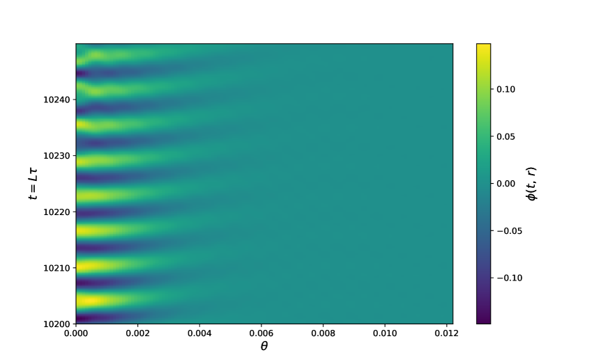
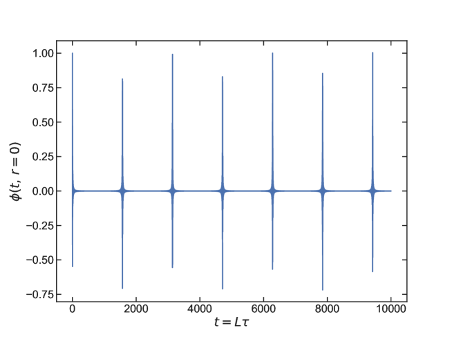
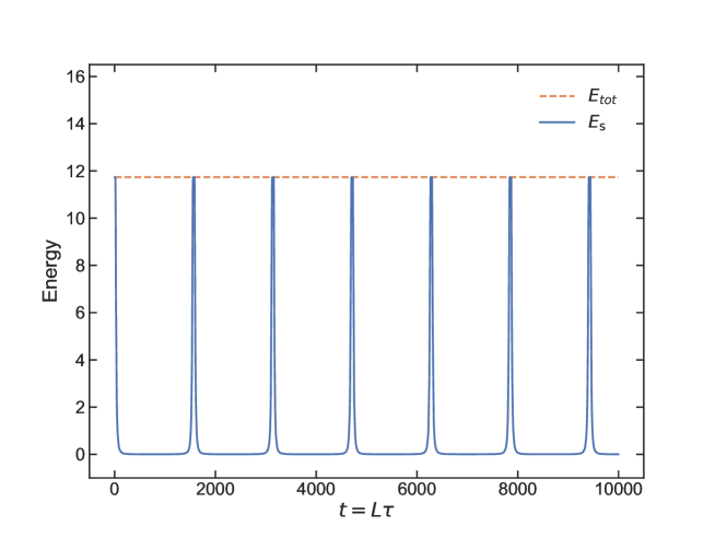
Figure 1 shows the time evolution of the field at with , and . To see the consistency of the computation, the time evolution of the total and shell energies is presented in Fig. 2. The orange line denotes the total energy in (2.13) and the blue line indicates the shell energy in (3.4) with . The total energy is well conserved and ensures the consistency of the numerical computation. To be more precise, we have checked that numerical errors are at the end of computation.
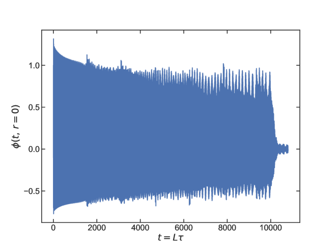
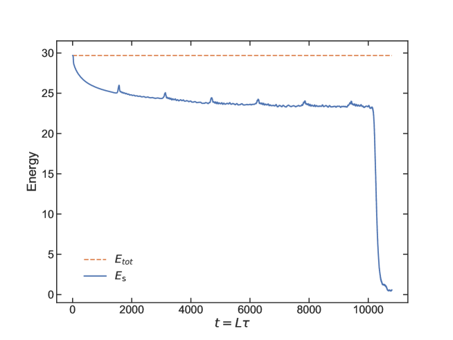
Seeing the behavior of , one can figure out the behavior of the solution. At first, a small amount of the energy escapes from the shell as radiation but most of remains inside the shell. By combining this observation with Fig. 1 , one can see that the excitation is well localized around . Then, the field begins and continues to oscillate for a long time. This is a characteristic feature of the oscillon and is called the oscillon regime. Finally, the localized excitation decays around and all remaining energy is abruptly emitted from the shell. This is a typical behavior of the oscillon as in the Minkowski case [3].
Note that there are some small bumps in the oscillon regime before the decay. These are radiations emitted at the beginning of time evolution and reflected by the AdS curvature effect. The traveling time is estimated as . Now it is and nicely agrees with the periodicity in Fig. 1. This is a characteristic behavior intrinsic to the AdS space.
3.3 Recurrence
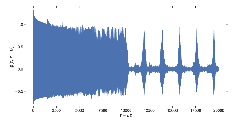
Another characteristic of our setup can be seen by extending the computation time. The other parameters are the same as for Fig. 1. The result is plotted in Fig. 3. Now one can see new peaks after the end of the oscillon regime. To interpret them, it is useful to look at Fig. 4 . By seeing the blue line, one can see that the energy released as radiation after the decay returns to periodically. The periodicity agrees with again as small bumps in the oscillon regime. This can be understood as the phenomenon of recurrence.
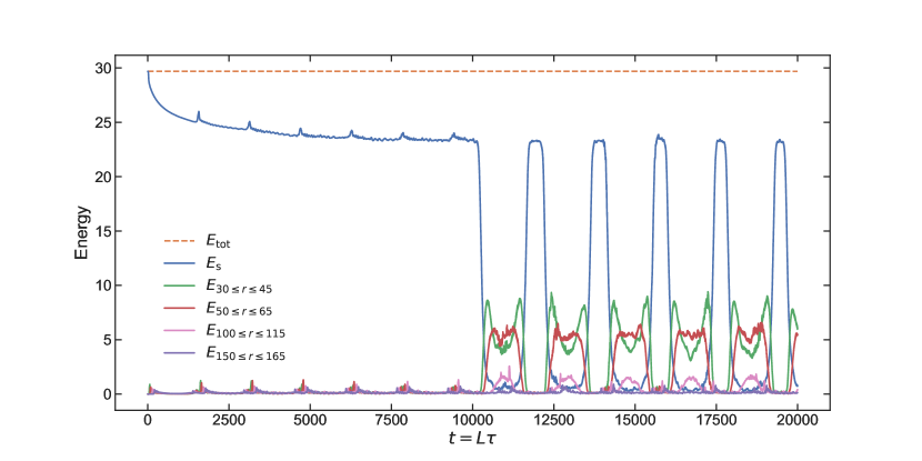
As a possibility, one might think that a localized lump begins to move without decay and then is reflected to . However, this can be excluded by seeing the green, red, pink and purple lines in Fig. 4 . These denote the behavior of energies in different integral regions. Each energy is defined as
| (3.6) |
As a result, the behaviors indicate that there is no localized lump. This observation can also be seen from Fig. 5. This is a magnified plot around the oscillon decay. One can see that the oscillon emits radiation and tends to decay.
It is also interesting to see the recurrence phenomenon for non-oscillon configuration. In the Minkowski case, the bound for possible size of the oscillon core was evaluated in [3]. This analysis can be generalized to the AdS case and the bound for the oscillon core size is given by333This is the condition for the case with . In the AdS case, negative values of are possible if they satisfy the Breitenlohner-Freedman (BF) bound [7]. It is intriguing to study the oscillon in the regime with . We will leave it as a future issue.
| (3.7) |
and this condition provides a necessary condition for the existence of oscillon. By taking the limit, the Minkowski result [3] is reproduced. When and , the bound becomes . In the previous computation, we took and the condition (3.7) was satisfied. By taking a value of , one can generate non-oscillon solution. Figures 6 and 7 show the results for non-oscillons . One can see that the localized lump decays immediately and all energy can be emitted as radiations. Then the radiations are reflected to periodically with period . Thus, the recurrence can still be observed for non-oscillons and hence is not intrinsic to the oscillons.
Finally, it should be mentioned that the phenomenon of the recurrence is rather surprising, because the system we are considering is not integrable even if the AdS space can be seen as a box. A typically expected behavior should be turbulent. At least so far, we have no idea to explain why the recurrence occurs even for non-oscillon configurations. It is the most significant issue to reveal the fundamental mechanism for the recurrence as well as the longevity of the oscillon.
4 Conclusion and Discussion
We have studied oscillons in a real scalar field theory in a (3+1)-dimensional AdS space with the global coordinates. By supposing the same conditions as in the case of Minkowski spacetime, such as the Gaussian shape, we have constructed numerical oscillon solutions with longevity. In particular, since the AdS space can be seen as a box, the recurrence phenomenon has been observed under suitable conditions.
It may be interesting to consider an extension of the oscillon solution by including the gravitational backreaction for the AdS space by following the analysis [8]. The time-periodic solutions are constructed in [9] (for a nice review, see [10]). The truly localized and time-periodic solutions in the AdS space without backreaction have already been discussed in [11].
It is a fascinating issue to consider the dual gauge-theory interpretation of the oscillons (and extended ones with back reactions) via the AdS/CFT correspondence [12]. There are some speculations and open problems. First, it may be interesting to consider a static string in an AdS space as discussed in [13, 14, 15]. In this setup, real massive scalar field theories are realized in a two-dimensional AdS space and non-trivial potentials also appear by keeping some corrections in the semi-classical approximation. It is an intriguing challenge to look for an oscillon solution in this system. If it exists, it should be dual to a long-lived fluctuation of a Wilson loop [16, 17] on the gauge-theory side [18].
As a generalization in this direction, it is also possible to consider an AdS-brane in a higher-dimensional AdS space, which is a D-brane whose shape is AdS (called the AdS-brane). Similarly, real massive scalar field theories with a non-trivial potential can also be realized on the AdS-brane as well [15]. There may also exist oscillon-like excitations on the brane and these should be dual to non-trivial fluctuations of the dual object such as (dual) giant Wilson loops [19, 20, 21, 22] and conformal defects [23].
As an application of the oscillons in the AdS space, it is nice to consider the AdS/QCD setup as discussed in [24, 25]. In this direction, we first need to construct an oscillon in Poincare AdS space. Then it is also necessary to somehow engineer the dilaton potential to support it. If such a oscillon could be realized, its gauge-theory dual would be related to the dynamics of a glueball-like excitation. This is a fascinating and ambitious research subject.
The most important question is what is the underlying mechanism that ensures the oscillon longevity. Nobody knows the answer, at least for now. There may be a hidden symmetry behind the oscillon longevity, such as the Laplace-Runge-Lenz vector. In the presence of mass terms, the free part is regarded as a collection of harmonic oscillators, and such a symmetry may approximately survive. In this direction, the work [26] may be relevant.
Also, recently, there was an interesting approach to try to explain the oscillon longevity from the viewpoint of sphaleron [27] in a real scalar field theory with a cubic potential in two-dimensional Minkowski spacetime [28]. It is interesting to generalize the work [28] to a two-dimensional AdS space.
The mechanism to ensure oscillon longevity might be enlightened by the AdS/CFT correspondence. We hope that our work will be a first step in this direction.
Acknowledgments
The authors thank Henry Liao for useful discussions and comments. The work of T. I. was supported by JSPS Grant-in-Aid for Scientific Research (C) No. 19K03871. The works of T. M. and K. Y. were supported by MEXT KAKENHI Grant-in-Aid for Transformative Research Areas A “Machine Learning Physics” No. 22H05115, and JSPS Grant-in-Aid for Scientific Research (B) No. 22H01217.
Appendix
Appendix A Rescaling of the Lagrangian
To perform numerical computations, let us rewrite the Lagrangian in (2.3) ,
| (A.1) |
into the dimensionless form.
First of all, the coordinates and are made dimensionless by using the mass as
| (A.2) |
where and are dimensionless time and radial coordinates. Note here that this rescaling is intrinsic to the massive case.
Then, the curvature radius and the coupling constants and are also rescaled as
| (A.3) |
and the dimensionless field is defined as
| (A.4) |
Finally, by adjusting the overall constant, the dimensionless Lagrangian is given by
| (A.5) |
where .
In the main text, all the hats have been removed for brevity.
References
- [1] G. H. Derrick, “Comments on nonlinear wave equations as models for elementary particles,” J. Math. Phys. 5 (1964), 1252-1254.
- [2] M. Gleiser, “Pseudostable bubbles,” Phys. Rev. D 49 (1994), 2978-2981 [arXiv:hep-ph/9308279 [hep-ph]].
- [3] E. J. Copeland, M. Gleiser and H. R. Muller, “Oscillons: Resonant configurations during bubble collapse,” Phys. Rev. D 52 (1995), 1920-1933 [arXiv:hep-ph/9503217 [hep-ph]].
- [4] M. Gleiser and D. Sicilia, “Analytical Characterization of Oscillon Energy and Lifetime,” Phys. Rev. Lett. 101 (2008), 011602 [arXiv:0804.0791 [hep-th]].
- [5] M. Gleiser and D. Sicilia, “A General Theory of Oscillon Dynamics,” Phys. Rev. D 80 (2009), 125037 [arXiv:0910.5922 [hep-th]].
- [6] P. Dorey, T. Romanczukiewicz, Y. Shnir and A. Wereszczynski, “Oscillons in gapless theories,” Phys. Rev. D 109 (2024) no.8, 085017 [arXiv:2312.05308 [hep-th]].
- [7] P. Breitenlohner and D. Z. Freedman, “Positive energy in anti-de sitter backgrounds and gauged extended supergravity,” Phys. Lett. B 115 (1982), 197.
- [8] P. Bizon and A. Rostworowski, “On weakly turbulent instability of anti-de Sitter space,” Phys. Rev. Lett. 107 (2011), 031102 [arXiv:1104.3702 [gr-qc]].
- [9] M. Maliborski and A. Rostworowski, “Time-Periodic Solutions in an Einstein AdS Massless-Scalar-Field System,” Phys. Rev. Lett. 111 (2013), 051102 [arXiv:1303.3186 [gr-qc]].
- [10] G. T. Horowitz and J. E. Santos, “Geons and the instability of anti-de Sitter spacetime,” Surveys Diff. Geom. 20 (2015) no.1, 321-335 [arXiv:1408.5906 [gr-qc]].
- [11] G. Fodor, P. Forgács and P. Grandclément, “Scalar field breathers on anti-de Sitter background,” Phys. Rev. D 89 (2014) no.6, 065027 [arXiv:1312.7562 [hep-th]].
- [12] J. M. Maldacena, “The Large N limit of superconformal field theories and supergravity,” Adv. Theor. Math. Phys. 2 (1998), 231-252 [arXiv:hep-th/9711200 [hep-th]].
- [13] N. Drukker, D. J. Gross and A. A. Tseytlin, “Green-Schwarz string in AdSS5: Semiclassical partition function,” JHEP 04 (2000), 021 [arXiv:hep-th/0001204 [hep-th]].
- [14] J. Gomis, J. Gomis and K. Kamimura, “Non-relativistic superstrings: A New soluble sector of AdSS5,” JHEP 12 (2005), 024 [arXiv:hep-th/0507036 [hep-th]].
- [15] M. Sakaguchi and K. Yoshida, “Non-relativistic string and D-branes on AdSS5 from semiclassical approximation,” JHEP 05 (2007), 051 [arXiv:hep-th/0703061 [hep-th]].
- [16] S. J. Rey and J. T. Yee, “Macroscopic strings as heavy quarks in large N gauge theory and anti-de Sitter supergravity,” Eur. Phys. J. C 22 (2001) 379 [arXiv:hep-th/9803001].
- [17] J. M. Maldacena, “Wilson loops in large N field theories,” Phys. Rev. Lett. 80 (1998) 4859 [arXiv:hep-th/9803002].
- [18] M. Sakaguchi and K. Yoshida, “Holography of Non-relativistic String on AdSS5,” JHEP 02 (2008), 092 [arXiv:0712.4112 [hep-th]].
- [19] N. Drukker and B. Fiol, “All-genus calculation of Wilson loops using D-branes,” JHEP 02 (2005), 010 [arXiv:hep-th/0501109 [hep-th]].
- [20] S. Yamaguchi, “Wilson loops of anti-symmetric representation and D5-branes,” JHEP 05 (2006), 037 [arXiv:hep-th/0603208 [hep-th]].
- [21] J. Gomis and F. Passerini, “Holographic Wilson Loops,” JHEP 08 (2006), 074 [arXiv:hep-th/0604007 [hep-th]].
- [22] J. Gomis and F. Passerini, “Wilson Loops as D3-Branes,” JHEP 01 (2007), 097 [arXiv:hep-th/0612022 [hep-th]].
- [23] O. DeWolfe, D. Z. Freedman and H. Ooguri, “Holography and defect conformal field theories,” Phys. Rev. D 66 (2002), 025009 [arXiv:hep-th/0111135 [hep-th]].
- [24] U. Gursoy and E. Kiritsis, “Exploring improved holographic theories for QCD: Part I,” JHEP 02 (2008), 032 [arXiv:0707.1324 [hep-th]].
- [25] U. Gursoy, E. Kiritsis and F. Nitti, “Exploring improved holographic theories for QCD: Part II,” JHEP 02 (2008), 019 [arXiv:0707.1349 [hep-th]].
- [26] O. Evnin and C. Krishnan, “A Hidden Symmetry of AdS Resonances,” Phys. Rev. D 91 (2015) no.12, 126010 [arXiv:1502.03749 [hep-th]].
- [27] F. R. Klinkhamer and N. S. Manton, “A Saddle Point Solution in the Weinberg-Salam Theory,” Phys. Rev. D 30 (1984), 221.
- [28] N. S. Manton and T. Romańczukiewicz, “Simplest oscillon and its sphaleron,” Phys. Rev. D 107 (2023) no.8, 085012 [arXiv:2301.09660 [hep-th]].