TU-1253
KEK-QUP-2024-0029
Domain walls in Nelson-Barr axion model
Kai Murai(a)***kai.murai.e2@tohoku.ac.jp and Kazunori Nakayama(a,b)†††kazunori.nakayama.d3@tohoku.ac.jp
(a)Department of Physics, Tohoku University, 6-3 Aoba, Aramaki, Aoba-ku, Sendai, Miyagi 980-8578, Japan
(b)International Center for Quantum-field Measurement Systems for Studies of the Universe and Particles (QUP), KEK, 1-1 Oho, Tsukuba, Ibaraki 305-0801, Japan
We explore a concrete realization of a Nelson-Barr model addressing the strong CP problem with suppressed unfavorable corrections. This model has a scalar field that spontaneously breaks discrete symmetry, and its phase component can naturally be relatively light, which we call the Nelson-Barr axion. It has both a tree-level potential and the QCD instanton-induced potential like the QCD axion, each minimizing at the CP-conserving point. While one potential leads to domain wall formation, the other works as a potential bias. This model provides a natural setup for the collapse of the axion domain walls by a potential bias without spoiling a solution to the strong CP problem. We discuss the cosmological implications of domain wall collapses, including dark matter production and gravitational wave emission.
1 Introduction
The strong CP problem remains one of the unresolved issues in the Standard Model (see, e.g., Refs. [1, 2] for reviews). Quantum chromodynamics (QCD) generally includes a CP-violating term with and being the field strength of the gluon and its dual, respectively. Considering the chiral rotation of the quark phases, the CP violation is described by an invariant angle of
| (1) |
where and are the mass matrices of the up- and down-type quarks, respectively. From the perspective of naturalness, is expected to be of . On the other hand, the measurement of the neutron electric dipole moment imposes a stringent limit of [3]. This discrepancy is called the strong CP problem, and various solutions have been suggested. Among them, there are two well-known classes of solutions to the strong CP problem:111 The solution with the massless up-quark [4, 5, 6, 7] is currently disfavored by the results of lattice QCD [8, 9, 10]. the Peccei-Quinn mechanism [11, 12] with the QCD axion [13, 14] and the spontaneous or soft breaking of a discrete spacetime symmetry such as parity [15, 16, 17, 18] or CP symmetry [19, 20, 21, 22, 23, 24].
In the Nelson-Barr mechanism [22, 23], one realization of the latter idea, the fundamental theory is exactly symmetric under a CP transformation, and thus at the Lagrangian level. With a specific structure of the mass matrix, the CP-violating angle in the Cabibbo-Kobayashi-Maskawa (CKM) matrix can be reproduced while keeping the smallness of . The class of the Nelson-Barr model and its extensions remain an active field of research even in this decades (see, e.g., Refs. [25, 26, 27, 28, 29, 30, 31, 32, 33, 34, 35, 36, 37, 38, 39, 40, 41, 42, 43, 44]).
Recently, we proposed a modification of the minimal realization of the Nelson-Barr mechanism. Compared to the original model proposed by Bento, Branco, and Parada (BBP) [24], we introduced an approximate discrete symmetry, , to the model. Thanks to this symmetry, unfavorable contributions to from loop diagrams and higher-order operators are highly suppressed by a small parameter . As a result, we can safely realize a high scale of spontaneous CP breaking GeV, which is compatible with the required temperature GeV [45, 46] for the thermal leptogenesis scenario [47]. While the previous work investigated the requirement for the model parameters including , the model was presented as an effective theory, and its concrete realization was not discussed in detail.
In this paper, we propose one possible realization of the Nelson-Barr mechanism in Ref. [48]. The soft breaking of the additional symmetry is described by the vacuum expectation value (VEV) of a complex scalar with a charge of . While the VEV of must be real to solve the strong CP problem, necessarily has multiple potential minima including complex ones due to the symmetry. Thus, cosmic strings and domain walls can be formed if acquires nonzero VEV after inflation, and is unfavorably large in all domains but . In this sense, the strong CP problem is solved with a probability of . Interestingly, the introduction of the complex scalar necessarily predicts something like the QCD axion. Since the complex scalar couples to quarks, the QCD non-perturbative effects induce a potential for its phase component. If the QCD potential is dominant over the tree-level potential, it is nothing but a QCD axion. In our case, the strong CP problem is solved via the Nelson-Barr mechanism even if the axion potential is dominated by the tree level one. We call it the Nelson-Barr axion.
We study the cosmology and phenomenology of the Nelson-Barr axion model. What we find are:
-
•
Compared with the conventional QCD axion models, the Nelson-Barr axion allows different parameter regions in terms of the mass and coupling strength.
-
•
Domain walls are formed when the symmetry is spontaneously broken. Such walls are unstable due to the potential bias given by the QCD effect. It may leave the observable gravitational wave signals.
-
•
Nelson-Barr axion can play the role of dark matter, either from the misalignment mechanism or the collapse of axionic domain walls.
The remarkable point of this model is that the collapse of axion domain walls can be realized without spoiling the quality of the QCD axion.222 The effect of the QCD potential as a bias on the domain wall has been discussed in Refs. [49, 50, 51, 52, 53, 54, 55, 56, 57, 58, 59, 60, 61]. This is in contrast to simple axion models, where an additional source of the axion potential for the domain wall collapse generally spoils the quality of the QCD axion unless a fine-tuning of the potential is assumed.
The rest of this paper is organized as follows. In Sec. 2, we briefly review the modified BBP model proposed in Ref. [48] and provide its concrete realization. We also discuss the emergence of the Nelson-Barr axion. In Sec. 3, we investigate the formation, evolution, and collapse of cosmic strings and domain walls and evaluate the axions and gravitational waves emitted from domain walls. Finally, we conclude and discuss our results in Sec. 4.
2 Realization of Nelson-Barr model and axion
2.1 Modified BBP model
First, we review the model in the Nelson-Barr framework proposed in Ref. [48], which is an extension of a minimal model of spontaneous CP violation [24]. In this model, we impose CP symmetry and introduce vector-like quarks and with the U(1) hypercharge of , right-handed neutrinos , and a singlet complex scalar as additional field contents to the Standard Model. The Lagrangian is given by
| (2) |
where , , , , , , , , are real constants due to the CP symmetry, and are the Standard Model right-handed down-type quarks, left-handed quark doublets, Higgs doublet, left-handed lepton doublets, and right-handed leptons, respectively. Note that the right-handed neutrinos are introduced to accommodate leptogenesis and are not essential to solve the strong CP problem. Here, we impose an exact symmetry and an approximate symmetry and assign their charges as shown in Table 1. While the former symmetry forbids the interaction terms such as , the latter forbids the terms with , which can be regarded as a spurion field with a charge under the symmetry. We consider that is softly broken, and . Due to the smallness of , this model is free from the quality problem in the Nelson-Barr models.
The scalar potential is given by
| (3) |
where all coefficients are real due to the CP symmetry, and GeV and are the VEVs of and , respectively. For simplicity, we assume that the terms in the second line are smaller than those in the first line so that the VEVs of and are mostly determined by the first line. With this potential, the VEV of is given by , where the complex phase can take an arbitrary value depending on the choice of coefficients of the and terms. This is the source of spontaneous CP violation.
If acquires the nonzero VEV after inflation, domain walls are formed at the spontaneous symmetry breaking and may alter the expansion history of the later universe. We can avoid such a situation by requiring a low reheating temperature so that the symmetry is not restored after inflation. Instead, we can assure that the symmetry remains spontaneously broken after inflation by assuming negative Hubble and thermal mass potentials for with [48]. Note that the latter approach allows a high reheating temperature, which is required for thermal leptogenesis.
Then, the mass matrix of the quarks can be written as
| (4) |
where and . Here, is complex while and are real. Thus, , and the strong CP angle vanishes at the tree level. On the other hand, the CP phase in the CKM matrix appears after diagonalizing this mass matrix. To reproduce CP phase in the CKM matrix while keeping the unitarity of the CKM matrix, we require and [48].
When we take into account higher-order operators and loop effects, there are additional contributions to the strong CP angle. One possible operator contributing to the strong CP angle is given by
| (5) |
with cutoff scale and being real constants. Due to the symmetry, this operator is suppressed by . Furthermore, there are loop contributions to the strong CP angle, which is estimated as [48]
| (6) |
where and are the masses of the Higgs particle and the angular component of , respectively. These additional contributions to are suppressed by and are safely small, , with sufficiently small even if the model parameters such as , , , and are not tuned. This is an advantage of the modified model [48] compared to the original setup [24].
2.2 Concrete realization of the modified BBP model
2.2.1 Model description
So far, the small parameter is an effective parameter that describes the small explicit breaking of the symmetry. Next, we provide a concrete realization of this model. We assume that the symmetry is not explicitly broken but only spontaneously broken by a complex scalar . The Lagrangian is given by
| (7) |
where we omitted the lepton sector, which is the same as in the previous subsection. Again all coefficients are real since the CP symmetry is imposed. We assume that the mass parameter is of the same order as the mass parameters in the scalar potential and is much smaller than the cutoff scale . The charges of the fields are summarized in Table 2. The potential for is given by
| (8) |
where and are real constants, and is the VEV of . When has a real VEV, we can regard in the previous model.333 A similar idea in the context of flavor symmetry to explain the hierarchical Yukawa structure is known as the Froggatt-Nielsen mechanism [62]. The second term explicitly breaks a U(1) symmetry associated with , and ensures that has a potential minimum on its real axis. We assume , and then the potential minimum is given by
| (9) |
with
| (10) |
The strong CP angle is zero at the tree level if we live in the universe with . Otherwise, there appears a large strong CP angle inconsistent with experiments. In this sense, the solution to the strong CP problem may work with a probability of , if we start with one of these vacua during inflation. However, as we will see below, there is a dynamical mechanism to choose the CP-conserving vacuum .
Let us comment on the “quality” of the CP conservation at the vacuum . Actually, the reality of the VEV of should not be exact, but there are several terms that cause a deviation from . One possible term is , but it does not cause such a deviation if the coefficient of this term is negative. Moreover, even if the coefficient is positive, it is suppressed by compared with the original term, and hence the effect of this term is negligible. On the other hand, terms such as cause deviation from ; we may have at the true minimum. This is of the same order as the loop-induced strong CP angle, and it gives a strong constraint on our model parameters.
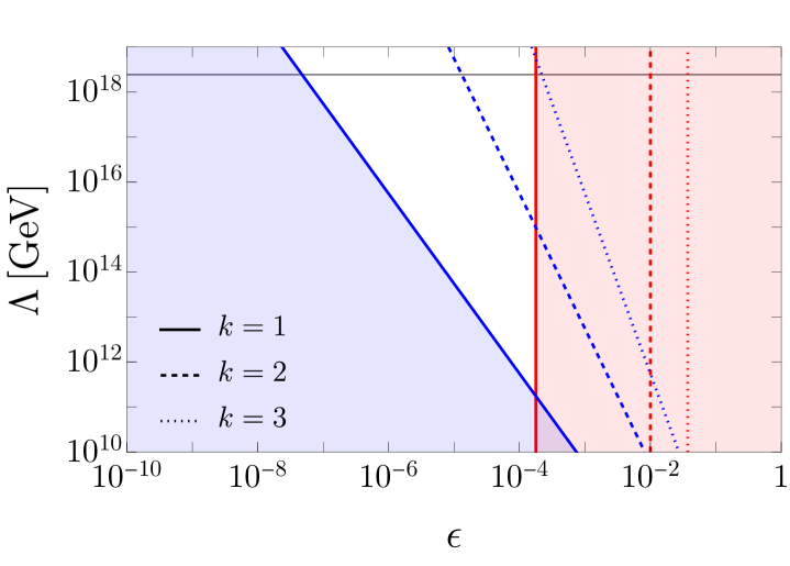
Here we summarize the conditions for the model parameter following Ref. [48]. For simplicity, we assume and in the following. To solve the strong CP problem, should be sufficiently small: and . In addition, to reproduce the CKM matrix, we require and . Then, we obtain the conditions of
| (13) |
where GeV is the reduced Planck mass. We show the favored range of in Fig. 1. For example, when and , the constraint on is given by
| (14) |
2.2.2 Appearance of Nelson-Barr axion
In our model we have a complex scalar that couples to quarks. Thus its angular component obtains mass from the QCD effect. As a canonical degree of freedom, we define . Then, non-perturbative effects of the QCD induce a potential of
| (15) |
where is the topological susceptibility of the QCD and depends on temperature as
| (18) |
In the following, we adopt , , and [63]. Taking into account the tree-level term in , the total potential for is given by
| (19) |
where . If the QCD-induced potential is dominant over the tree-level potential, may be identified with the QCD axion. In such a case, we do not need to impose the CP symmetry to solve the strong CP problem. However, in our model, the strong CP problem is solved via the Nelson-Barr mechanism even if the QCD-induced potential is subdominant. In this sense, we do not require the “quality” of the approximate U(1) symmetry at the level of conventional QCD axion models. We call the Nelson-Barr axion in such a case. It leads to rich phenomenology.444 Ref. [43] also considered axion-like particle in the Nelson-Barr model. In their model the axion is a phase of field by imposing U(1) symmetry with high quality and it is anomaly-free under the QCD.
We briefly comment on the cosmology of the present model. First let us consider a scenario where the symmetry is restored during inflation and spontaneously broken at some epoch well after inflation. Then the network of cosmic strings and domain walls is formed, in which each string is attached by domain walls. This network is stable if were absent. Due to , which works as a bias potential, the string-wall network finally collapses unless the two terms in have degenerate minima at . In the following, we require that and are coprime to each other so that the CP-conserving vacuum, , is finally realized in the whole universe. Therefore, in this scenario, takes the role of picking up a CP-conserving vacuum dynamically out of vacua. We discuss the cosmological implications of such a scenario in the next section in detail.
On the other hand, if the symmetry is already broken during inflation, the field value of is effectively uniform at the end of inflation. To solve the strong CP problem, must settle to , which is realized with a probability of when we consider . If is sufficiently larger than the tree level potential, finally settles to and the strong CP problem is solved, although the Nelson-Barr mechanism is irrelevant. In this case, the axion is trapped in a local minimum for a while and then starts to oscillate around the true vacuum as in the trapped misalignment mechanism [54, 64, 65, 66, 67, 68].
3 Cosmology of domain walls
Here, we assume that acquires a nonzero VEV after inflation and discuss the evolution of the string-wall network focusing on its cosmological implications.555 There are two types of domain walls: one is related to the breaking of and the other . The former is characterized by the VEV of , and we assume that continues to have a large VEV as in the scenario of Ref. [48]. Thus domain walls do not appear. We focus on the latter type of domain walls characterized by the VEV of . In the following, we assume the radiation-dominated universe in all the relevant epoch.
In our scenario, after the formation of cosmic strings, domain walls are formed when the axion mass overcomes the Hubble friction. Each cosmic string has domain walls attached to it and forms a string-wall network. The tensions of strings and walls are given as
| (20) |
respectively.
In contrast to the case with a domain wall number of unity, the string-wall network is long-lived and eventually set in the so-called scaling regime. In the scaling regime, there are strings and walls in each Hubble volume. Thus, the energy densities of strings and walls evolve as
| (21) |
respectively. Since decreases in time more slowly than , the energy density of the string-wall network is approximated by .
As the universe cools down, the potential from the QCD effect grows and works as a potential bias on the domain walls. The difference in the potential between two sides of a domain wall is evaluated as
| (22) |
where with . Note that and represent the same vacuum. Still there remains a degeneracy between and , which is ensured by the invariance under the CP transformation . However, the lowest energy vacuum is unique. In the following, we consider the case of and denote the typical bias by , while the bias depends on .666 Precisely speaking, the potential minimum slightly deviates from as mentioned in Sec. 2.2.1, but the CP also transforms the phase of as . Thus the degenerate potential minima are separated by the domain wall, which is irrelevant in our cosmological scenario.
The string-wall network collapses when this pressure overcomes the domain wall tension force, i.e.,
| (23) |
where is the cosmic time when the network collapses, and is an area parameter representing the number of domain walls in each Hubble volume. Although evolves in time [69, 70] and depends on the initial conditions of [71] in general, in the following, we set for simplicity. Thus, we can evaluate as
| (24) |
where is the cosmic temperature at . From the relation during the radiation-dominated era, , and the Friedmann equation, we obtain
| (27) |
For the domain wall network to collapse before the big bang nucleosynthesis, we require MeV, which leads to the upper bound on of
| (28) |
We also require that the domain walls decay before they dominate the universe. This condition leads to the upper bound of
| (29) |
Note that the potential bias is at most , which is smaller than the total energy density at , and thus the domain walls collapse at when saturates this upper limit.
3.1 Dark matter production
First, we evaluate the dark matter abundance emitted from the domain wall collapse following Ref. [72]. Even in the scaling regime, the comoving number density of domain walls decreases emitting axion particles. Since, in the scaling regime, the energy density of the domain walls decreases more slowly than non-relativistic matter, the axion abundance after the domain wall collapse is mainly contributed by particle production during the network collapse. Here, we evaluate the axion abundance assuming that the axion particle is stable.
In the scaling regime during the radiation-dominated era, the domain walls emit axion particles at the rate of
| (30) |
Note that this rate does not include the decrease in due to cosmic expansion, and we neglected the decrease due to gravitational wave emission, which is negligibly small. We parameterize the average energy of emitted axions by
| (31) |
where we assume to be a constant. Here, we also assume that the axion mass can be approximated by for any temperatures although can substantially contribute to the axion mass in general as we will see later. Then, the axion number density emitted from the domain walls is evaluated as
| (32) |
for . Thus, the energy density from the domain wall collapse is given by
| (33) |
after the emitted axions become non-relativistic. Thus, we can evaluate the ratio of the energy density of to the entropy density as
| (34) |
for . If eV (see, e.g., Ref. [73]), the axion emitted from the domain wall can explain all dark matter.
In addition to the contribution from the domain wall collapse, the axion is generated from the misalignment mechanism. If we neglect , we can evaluate the axion abundance from the misalignment mechanism as [74]
| (35) |
where is the reduced Hubble constant, and is the initial value of , and the angle bracket denotes the spatial average. In our case, we obtain
| (36) |
3.2 Gravitational wave production
In the scaling regime, the string-wall network also emits gravitational waves. Here, we evaluate the spectrum of the gravitational waves following Ref. [70]. As in the case of the axion emission, the dominant contribution comes from just before and during the network collapse. Since the frequency of the gravitational waves is determined by the Hubble scale at the emission, the peak frequency of the total gravitational spectrum is estimated by
| (37) |
at . The peak value of the density parameter of the gravitational waves, , is estimated as
| (38) |
where is an efficiency parameter of the gravitational wave emission.
Taking into account the redshift after the emission, for , we obtain the peak frequency at the current time as
| (39) |
and the peak of the current gravitational wave spectrum as
| (40) |
where K is the current CMB temperature [75] and is the current density parameter of radiation [73]. According to numerical simulations, the gravitational wave spectrum around the peak follows for and for [70]. Interestingly, if the domain walls collapse around the QCD phase transition epoch thanks to the QCD potential bias, the peak frequency is predicted to be nHZ range, which is the range of pulsar timing array experiments [52, 58, 59].
3.3 Model predictions
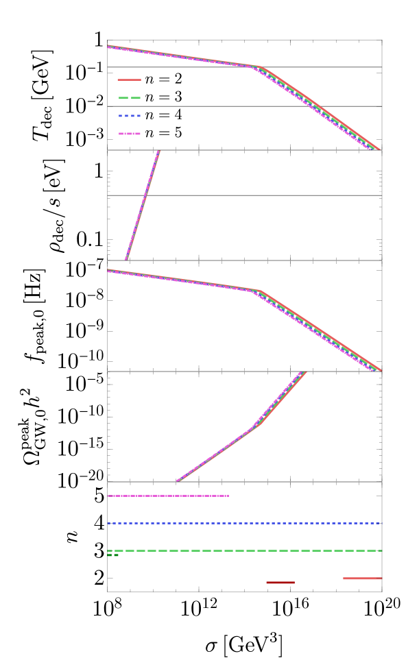
As seen in the previous section, the production of the axion and gravitational waves is mainly controlled by the domain wall tension, . We show the dependence of , , , and on in Fig. 2. In the bottom plot, we also show the allowed region for under the limit on in Eq. (13). Here, we adopted the fitting function of and presented in Ref. [76]. While all dark matter can be produced for , the abundance of the gravitational waves is much smaller than the observable range for such .
Once we fix and , we can relate to via Eq. (20), leading to and . Then, we can estimate the mass and couplings of the axion. The axion mass is determined by the two contributions in (see Eq. (19)). For , the axion mass squared is given by
| (41) |
Regarding the couplings of the axion, we expect that the axion is coupled to the standard model particles as the QCD axion. In particular, we assume the axion-photon coupling of
| (42) |
with
| (43) |
Here, and are the field strength of the photon and its dual, and is the fine-structure constant.
First, we fix and discuss the production of axion dark matter. We show the prediction for in this case in Fig. 3.
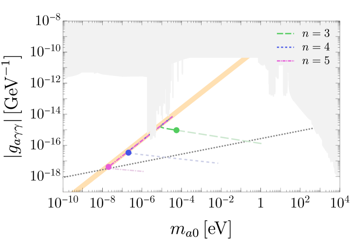
The colored lines denote the prediction of this scenario. Due to the contribution of , the axion can be heavier than the QCD band. On the other hand, when is smaller than the contribution from , the prediction is aligned with the QCD band. At the colored circles, the axions emitted from the domain wall collapse can account for all dark matter. For these parameters, the contribution of to the axion mass is not dominant, and thus the temperature dependence of the axion mass does not affect the estimate of the axion abundance significantly. Note that on the heavier side of the circles, shown in lighter colors, the produced axions exceed the dark matter abundance, and thus it should decay via some processes, although our model does not include such decay channels as it is. The gray-dotted line represents the parameter with which the contribution from the misalignment mechanism (35) matches the observed abundance of dark matter. While the contributions from the domain wall collapse and misalignment mechanism can comparably contribute to all dark matter for , the former contribution will be dominant for and .777 Here we have implicitly assumed a cosmological scenario with domain wall formation. If the symmetry is already broken during inflation, there are no domain walls at all. In such a case, the misalignment mechanism is the dominant dark matter production mechanism.
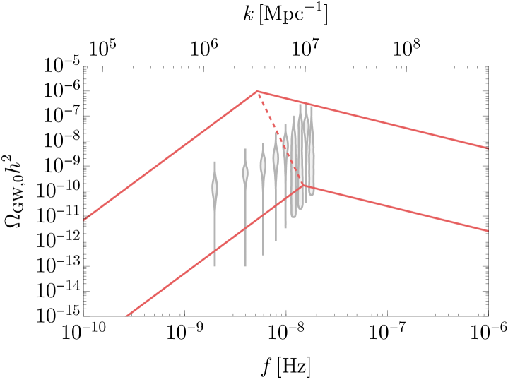
Next, we consider GeV and discuss the generation of gravitational waves. We show the current power spectrum of the gravitational waves from the domain wall collapse in Fig. 4. Here, we assume , , , and . The red lines denote the maximum and minimum power spectrum of the gravitational waves coming from the bound on (13) and the requirement for the domain wall collapse before domination (29). Within this range, the gravitational waves from the domain wall collapse can explain the signal reported by the NANOGrav 15 yr result [78].888 The explanation of the NANOGrav result by the domain wall collapse due to the QCD potential is also numerically studied in Ref. [59].
We also show the corresponding range of the mass and photon coupling in Fig. 5.
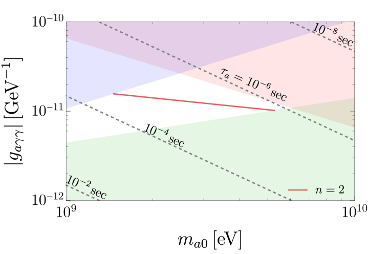
The gray-dashed lines represent the contours of the axion lifetime, . The decay rate of the heavy axion with GeV is estimated by
| (44) |
where is the strong coupling constant. Here, we adopt as a typical value for the scale of GeV [79]. The axion lifetime for the parameters of interest is shorter than sec, which corresponds to the Hubble time at the domain wall collapse, GeV (see Fig. 2). Thus, the axions will immediately decay after emitted from the domain wall collapse. In the colored regions, is too large (red), the CKM matrix cannot be reproduced (blue), and the domain walls dominate the universe before the decay (green). This shows that the parameter region for reproducing the NANOGrav result may be verified by the future measurement of the strong CP angle or the non-unitarity of the CKM matrix (or the collider production of heavy quarks).
4 Conclusions and discussion
The BBP model [24] is a simple model that solves the strong CP problem through the Nelson-Barr mechanism, although there are several quality problems in the original setup. A modified BBP model proposed in Ref. [48] introduced an approximate symmetry to suppress several operators that cause quality problems. There a small explicit symmetry breaking parameter was introduced by hand. In this paper, we have considered a concrete realization of such a setup by introducing a complex scalar and assuming a spontaneous breaking of the symmetry due to the VEV of , rather than the explicit breaking. The small symmetry breaking parameter is replaced by the ratio of the VEV of and cutoff scale .
We have studied the cosmology and phenomenology of such a model. First, the phase of , , is relatively light due to the symmetry, and it can play the role of dark matter depending on the parameter choice. Interestingly, the phase of also obtains a mass from the QCD instanton effect in the same way as the QCD axion since necessarily couples to heavy quarks. In our model, the strong CP problem is solved even if the QCD instanton effect is much smaller than the tree-level potential. Still, the phase of shares several properties similar to the QCD axion, and hence we call it the Nelson-Barr axion. Compared with the conventional QCD axion, the Nelson-Barr axion can take different parameter ranges in terms of the mass and coupling strength (see Figs. 3 and 5).
Second, domain walls lead to several important consequences. In the present model, domain walls associated with the spontaneous breakdown of the symmetry are not stable due to the potential bias induced by the QCD instanton effect [49]. Thus domain walls eventually collapse and, as a result, the whole universe dynamically ends up with the CP-conserving vacuum . The phenomenological implications of domain wall collapse depend on the cutoff scale . If is huge (say, close to the Planck scale), it can produce the correct amount of Nelson-Barr axion dark matter. On the other hand, if is as small as GeV, it can explain the recent pulsar timing array data for the stochastic gravitational wave background. Note that, in the most previous models of collapsing domain walls with the QCD potential bias, the strong CP problem is a serious issue since the Peccei-Quinn mechanism does not work, and some non-trivial model extensions are required [49, 50, 51, 52, 53, 54, 55, 56, 57, 58, 59, 60, 61]. We emphasize that our model provides a natural realization of such a scenario without the strong CP problem; even if the QCD-induced potential for the Nelson-Barr axion is subdominant, the potential minimum is a CP-conserving point. Interestingly, the parameter region for reproducing the NANOGrav result is close to the current experimental bound from the measurement of the strong CP angle and the unitarity of the CKM matrix, as shown in Fig. 5. In other words, future improvements of these observables may verify or falsify this scenario.
Acknowledgment
This work was supported by World Premier International Research Center Initiative (WPI), MEXT, Japan. This work was also supported by JSPS KAKENHI (Grant Numbers 24K07010 [KN], 23KJ0088 [KM], and 24K17039 [KM]).
References
- [1] J. E. Kim and G. Carosi, “Axions and the Strong CP Problem,” Rev. Mod. Phys. 82 (2010) 557–602, arXiv:0807.3125 [hep-ph]. [Erratum: Rev.Mod.Phys. 91, 049902 (2019)].
- [2] A. Hook, “TASI Lectures on the Strong CP Problem and Axions,” PoS TASI2018 (2019) 004, arXiv:1812.02669 [hep-ph].
- [3] C. Abel et al., “Measurement of the Permanent Electric Dipole Moment of the Neutron,” Phys. Rev. Lett. 124 no. 8, (2020) 081803, arXiv:2001.11966 [hep-ex].
- [4] H. Georgi and I. N. McArthur, “INSTANTONS AND THE mu QUARK MASS,”.
- [5] D. B. Kaplan and A. V. Manohar, “Current Mass Ratios of the Light Quarks,” Phys. Rev. Lett. 56 (1986) 2004.
- [6] K. Choi, C. W. Kim, and W. K. Sze, “Mass Renormalization by Instantons and the Strong CP Problem,” Phys. Rev. Lett. 61 (1988) 794.
- [7] T. Banks, Y. Nir, and N. Seiberg, “Missing (up) mass, accidental anomalous symmetries, and the strong CP problem,” in 2nd IFT Workshop on Yukawa Couplings and the Origins of Mass, pp. 26–41. 2, 1994. arXiv:hep-ph/9403203.
- [8] Z. Fodor, C. Hoelbling, S. Krieg, L. Lellouch, T. Lippert, A. Portelli, A. Sastre, K. K. Szabo, and L. Varnhorst, “Up and down quark masses and corrections to Dashen’s theorem from lattice QCD and quenched QED,” Phys. Rev. Lett. 117 no. 8, (2016) 082001, arXiv:1604.07112 [hep-lat].
- [9] C. Alexandrou, J. Finkenrath, L. Funcke, K. Jansen, B. Kostrzewa, F. Pittler, and C. Urbach, “Ruling Out the Massless Up-Quark Solution to the Strong Problem by Computing the Topological Mass Contribution with Lattice QCD,” Phys. Rev. Lett. 125 no. 23, (2020) 232001, arXiv:2002.07802 [hep-lat].
- [10] Flavour Lattice Averaging Group (FLAG) Collaboration, Y. Aoki et al., “FLAG Review 2021,” Eur. Phys. J. C 82 no. 10, (2022) 869, arXiv:2111.09849 [hep-lat].
- [11] R. D. Peccei and H. R. Quinn, “CP Conservation in the Presence of Instantons,” Phys. Rev. Lett. 38 (1977) 1440–1443.
- [12] R. D. Peccei and H. R. Quinn, “Constraints Imposed by CP Conservation in the Presence of Instantons,” Phys. Rev. D 16 (1977) 1791–1797.
- [13] S. Weinberg, “A New Light Boson?,” Phys. Rev. Lett. 40 (1978) 223–226.
- [14] F. Wilczek, “Problem of Strong and Invariance in the Presence of Instantons,” Phys. Rev. Lett. 40 (1978) 279–282.
- [15] M. A. B. Beg and H. S. Tsao, “Strong P, T Noninvariances in a Superweak Theory,” Phys. Rev. Lett. 41 (1978) 278.
- [16] R. N. Mohapatra and G. Senjanovic, “Natural Suppression of Strong p and t Noninvariance,” Phys. Lett. B 79 (1978) 283–286.
- [17] K. S. Babu and R. N. Mohapatra, “A Solution to the Strong CP Problem Without an Axion,” Phys. Rev. D 41 (1990) 1286.
- [18] S. M. Barr, D. Chang, and G. Senjanovic, “Strong CP problem and parity,” Phys. Rev. Lett. 67 (1991) 2765–2768.
- [19] H. Georgi, “A Model of Soft CP Violation,” Hadronic J. 1 (1978) 155.
- [20] G. Segre and H. A. Weldon, “Natural Suppression of Strong and Violations and Calculable Mixing Angles in SU(2) X U(1),” Phys. Rev. Lett. 42 (1979) 1191.
- [21] S. M. Barr and P. Langacker, “A Superweak Gauge Theory of CP Violation,” Phys. Rev. Lett. 42 (1979) 1654.
- [22] A. E. Nelson, “Naturally Weak CP Violation,” Phys. Lett. B 136 (1984) 387–391.
- [23] S. M. Barr, “Solving the Strong CP Problem Without the Peccei-Quinn Symmetry,” Phys. Rev. Lett. 53 (1984) 329.
- [24] L. Bento, G. C. Branco, and P. A. Parada, “A Minimal model with natural suppression of strong CP violation,” Phys. Lett. B 267 (1991) 95–99.
- [25] L. Vecchi, “Spontaneous CP violation and the strong CP problem,” JHEP 04 (2017) 149, arXiv:1412.3805 [hep-ph].
- [26] M. Dine and P. Draper, “Challenges for the Nelson-Barr Mechanism,” JHEP 08 (2015) 132, arXiv:1506.05433 [hep-ph].
- [27] O. Davidi, R. S. Gupta, G. Perez, D. Redigolo, and A. Shalit, “Nelson-Barr relaxion,” Phys. Rev. D 99 no. 3, (2019) 035014, arXiv:1711.00858 [hep-ph].
- [28] J. Schwichtenberg, P. Tremper, and R. Ziegler, “A grand-unified Nelson–Barr model,” Eur. Phys. J. C 78 no. 11, (2018) 910, arXiv:1802.08109 [hep-ph].
- [29] A. L. Cherchiglia and C. C. Nishi, “Solving the strong CP problem with non-conventional CP,” JHEP 03 (2019) 040, arXiv:1901.02024 [hep-ph].
- [30] J. Evans, C. Han, T. T. Yanagida, and N. Yokozaki, “Complete solution to the strong problem: Supersymmetric extension of the Nelson-Barr model,” Phys. Rev. D 103 no. 11, (2021) L111701, arXiv:2002.04204 [hep-ph].
- [31] A. L. Cherchiglia and C. C. Nishi, “Consequences of vector-like quarks of Nelson-Barr type,” JHEP 08 (2020) 104, arXiv:2004.11318 [hep-ph].
- [32] G. Perez and A. Shalit, “High quality Nelson-Barr solution to the strong CP problem with ,” JHEP 02 (2021) 118, arXiv:2010.02891 [hep-ph].
- [33] A. L. Cherchiglia, G. De Conto, and C. C. Nishi, “Flavor constraints for a vector-like quark of Nelson-Barr type,” JHEP 11 (2021) 093, arXiv:2103.04798 [hep-ph].
- [34] A. Valenti and L. Vecchi, “The CKM phase and in Nelson-Barr models,” JHEP 07 no. 203, (2021) 203, arXiv:2105.09122 [hep-ph].
- [35] A. Valenti and L. Vecchi, “Super-soft CP violation,” JHEP 07 no. 152, (2021) 152, arXiv:2106.09108 [hep-ph].
- [36] K. Fujikura, Y. Nakai, R. Sato, and M. Yamada, “Baryon asymmetric Universe from spontaneous CP violation,” JHEP 04 (2022) 105, arXiv:2202.08278 [hep-ph].
- [37] S. Girmohanta, S. J. Lee, Y. Nakai, and M. Suzuki, “A natural model of spontaneous CP violation,” JHEP 12 (2022) 024, arXiv:2203.09002 [hep-ph].
- [38] J. McNamara and M. Reece, “Reflections on Parity Breaking,” arXiv:2212.00039 [hep-th].
- [39] P. Asadi, S. Homiller, Q. Lu, and M. Reece, “Chiral Nelson-Barr models: Quality and cosmology,” Phys. Rev. D 107 no. 11, (2023) 115012, arXiv:2212.03882 [hep-ph].
- [40] P. F. Perez, C. Murgui, and M. B. Wise, “Automatic Nelson-Barr solutions to the strong CP puzzle,” Phys. Rev. D 108 no. 1, (2023) 015010, arXiv:2302.06620 [hep-ph].
- [41] D. Suematsu, “CP issues in the SM from a viewpoint of spontaneous CP violation,” Phys. Rev. D 108 no. 9, (2023) 095046, arXiv:2309.04783 [hep-ph].
- [42] T. Banno, J. Hisano, T. Kitahara, and N. Osamura, “Closer look at the matching condition for radiative QCD parameter,” JHEP 02 (2024) 195, arXiv:2311.07817 [hep-ph].
- [43] M. Dine, G. Perez, W. Ratzinger, and I. Savoray, “Nelson-Barr ultralight dark matter,” arXiv:2405.06744 [hep-ph].
- [44] J. F. Bastos and J. I. Silva-Marcos, “Reducing Complex Phases and other Subtleties of CP Violation,” arXiv:2407.07158 [hep-ph].
- [45] G. F. Giudice, A. Notari, M. Raidal, A. Riotto, and A. Strumia, “Towards a complete theory of thermal leptogenesis in the SM and MSSM,” Nucl. Phys. B 685 (2004) 89–149, arXiv:hep-ph/0310123.
- [46] W. Buchmuller, P. Di Bari, and M. Plumacher, “Leptogenesis for pedestrians,” Annals Phys. 315 (2005) 305–351, arXiv:hep-ph/0401240.
- [47] M. Fukugita and T. Yanagida, “Baryogenesis Without Grand Unification,” Phys. Lett. B 174 (1986) 45–47.
- [48] K. Murai and K. Nakayama, “Revisiting the minimal Nelson-Barr model,” JHEP 11 (2024) 098, arXiv:2407.16202 [hep-ph].
- [49] J. Preskill, S. P. Trivedi, F. Wilczek, and M. B. Wise, “Cosmology and broken discrete symmetry,” Nucl. Phys. B 363 (1991) 207–220.
- [50] M. Dine and A. E. Nelson, “Dynamical supersymmetry breaking at low-energies,” Phys. Rev. D 48 (1993) 1277–1287, arXiv:hep-ph/9303230.
- [51] F. Riva, “Low-Scale Leptogenesis and the Domain Wall Problem in Models with Discrete Flavor Symmetries,” Phys. Lett. B 690 (2010) 443–450, arXiv:1004.1177 [hep-ph].
- [52] T. Moroi and K. Nakayama, “Domain Walls and Gravitational Waves after Thermal Inflation,” Phys. Lett. B 703 (2011) 160–166, arXiv:1105.6216 [hep-ph].
- [53] K. Hamaguchi, K. Nakayama, and N. Yokozaki, “NMSSM in gauge-mediated SUSY breaking without domain wall problem,” Phys. Lett. B 708 (2012) 100–106, arXiv:1107.4760 [hep-ph].
- [54] T. Higaki, K. S. Jeong, N. Kitajima, and F. Takahashi, “Quality of the Peccei-Quinn symmetry in the Aligned QCD Axion and Cosmological Implications,” JHEP 06 (2016) 150, arXiv:1603.02090 [hep-ph].
- [55] T. Higaki, K. S. Jeong, N. Kitajima, T. Sekiguchi, and F. Takahashi, “Topological Defects and nano-Hz Gravitational Waves in Aligned Axion Models,” JHEP 08 (2016) 044, arXiv:1606.05552 [hep-ph].
- [56] S. Chigusa and K. Nakayama, “Anomalous Discrete Flavor Symmetry and Domain Wall Problem,” Phys. Lett. B 788 (2019) 249–255, arXiv:1808.09601 [hep-ph].
- [57] C.-W. Chiang and B.-Q. Lu, “Testing clockwork axion with gravitational waves,” JCAP 05 (2021) 049, arXiv:2012.14071 [hep-ph].
- [58] R. Z. Ferreira, A. Notari, O. Pujolas, and F. Rompineve, “Gravitational waves from domain walls in Pulsar Timing Array datasets,” JCAP 02 (2023) 001, arXiv:2204.04228 [astro-ph.CO].
- [59] N. Kitajima, J. Lee, K. Murai, F. Takahashi, and W. Yin, “Gravitational waves from domain wall collapse, and application to nanohertz signals with QCD-coupled axions,” Phys. Lett. B 851 (2024) 138586, arXiv:2306.17146 [hep-ph].
- [60] Y. Bai, T.-K. Chen, and M. Korwar, “QCD-collapsed domain walls: QCD phase transition and gravitational wave spectroscopy,” JHEP 12 (2023) 194, arXiv:2306.17160 [hep-ph].
- [61] S. Blasi, A. Mariotti, A. Rase, and A. Sevrin, “Axionic domain walls at Pulsar Timing Arrays: QCD bias and particle friction,” JHEP 11 (2023) 169, arXiv:2306.17830 [hep-ph].
- [62] C. D. Froggatt and H. B. Nielsen, “Hierarchy of Quark Masses, Cabibbo Angles and CP Violation,” Nucl. Phys. B 147 (1979) 277–298.
- [63] S. Borsanyi et al., “Calculation of the axion mass based on high-temperature lattice quantum chromodynamics,” Nature 539 no. 7627, (2016) 69–71, arXiv:1606.07494 [hep-lat].
- [64] S. Nakagawa, F. Takahashi, and M. Yamada, “Trapping Effect for QCD Axion Dark Matter,” JCAP 05 (2021) 062, arXiv:2012.13592 [hep-ph].
- [65] L. Di Luzio, B. Gavela, P. Quilez, and A. Ringwald, “Dark matter from an even lighter QCD axion: trapped misalignment,” JCAP 10 (2021) 001, arXiv:2102.01082 [hep-ph].
- [66] K. S. Jeong, K. Matsukawa, S. Nakagawa, and F. Takahashi, “Cosmological effects of Peccei-Quinn symmetry breaking on QCD axion dark matter,” JCAP 03 no. 03, (2022) 026, arXiv:2201.00681 [hep-ph].
- [67] S. Nakagawa, F. Takahashi, M. Yamada, and W. Yin, “Axion dark matter from first-order phase transition, and very high energy photons from GRB 221009A,” Phys. Lett. B 839 (2023) 137824, arXiv:2210.10022 [hep-ph].
- [68] L. Di Luzio and P. Sørensen, “Axion production via trapped misalignment from Peccei-Quinn symmetry breaking,” JHEP 10 (2024) 239, arXiv:2408.04623 [hep-ph].
- [69] T. Hiramatsu, M. Kawasaki, K. Saikawa, and T. Sekiguchi, “Axion cosmology with long-lived domain walls,” JCAP 01 (2013) 001, arXiv:1207.3166 [hep-ph].
- [70] T. Hiramatsu, M. Kawasaki, and K. Saikawa, “On the estimation of gravitational wave spectrum from cosmic domain walls,” JCAP 02 (2014) 031, arXiv:1309.5001 [astro-ph.CO].
- [71] N. Kitajima, J. Lee, F. Takahashi, and W. Yin, “Stability of domain walls with inflationary fluctuations under potential bias, and gravitational wave signatures,” arXiv:2311.14590 [hep-ph].
- [72] M. Kawasaki, K. Saikawa, and T. Sekiguchi, “Axion dark matter from topological defects,” Phys. Rev. D 91 no. 6, (2015) 065014, arXiv:1412.0789 [hep-ph].
- [73] Planck Collaboration, N. Aghanim et al., “Planck 2018 results. VI. Cosmological parameters,” Astron. Astrophys. 641 (2020) A6, arXiv:1807.06209 [astro-ph.CO]. [Erratum: Astron.Astrophys. 652, C4 (2021)].
- [74] Particle Data Group Collaboration, S. Navas et al., “Review of particle physics,” Phys. Rev. D 110 no. 3, (2024) 030001.
- [75] D. J. Fixsen, “The Temperature of the Cosmic Microwave Background,” Astrophys. J. 707 (2009) 916–920, arXiv:0911.1955 [astro-ph.CO].
- [76] K. Saikawa and S. Shirai, “Primordial gravitational waves, precisely: The role of thermodynamics in the Standard Model,” JCAP 05 (2018) 035, arXiv:1803.01038 [hep-ph].
- [77] C. O’Hare, “cajohare/axionlimits: Axionlimits.” https://cajohare.github.io/AxionLimits/, July, 2020.
- [78] NANOGrav Collaboration, G. Agazie et al., “The NANOGrav 15 yr Data Set: Evidence for a Gravitational-wave Background,” Astrophys. J. Lett. 951 no. 1, (2023) L8, arXiv:2306.16213 [astro-ph.HE].
- [79] D. d’Enterria et al., “The strong coupling constant: state of the art and the decade ahead,” J. Phys. G 51 no. 9, (2024) 090501, arXiv:2203.08271 [hep-ph].