Comparative Performance Analysis of Quantum Machine Learning Architectures for Credit Card Fraud Detection

Abstract

As financial fraud becomes increasingly complex, effective detection methods are essential. Quantum Machine Learning (QML) introduces certain capabilities that may enhance both accuracy and efficiency in this area. This study examines how different quantum feature map and ansatz configurations affect the performance of three QML-based classifiers—the Variational Quantum Classifier (VQC), the Sampler Quantum Neural Network (SQNN), and the Estimator Quantum Neural Network (EQNN)—when applied to two non-standardized financial fraud datasets. Different quantum feature map and ansatz configurations are evaluated, revealing distinct performance patterns. The VQC consistently demonstrates strong classification results, achieving an F1 score of 0.88, while the SQNN also delivers promising outcomes. In contrast, the EQNN struggles to produce robust results, emphasizing the challenges presented by non-standardized data. These findings highlight the importance of careful model configuration in QML-based financial fraud detection. By showing how specific feature maps and ansatz choices influence predictive success, this work guides researchers and practitioners in refining QML approaches for complex financial applications.

I Introduction

Credit card fraud represents a pervasive and escalating global threat, costing individuals and organizations billions of dollars each year. For instance, a 2022 UK Finance study reported fraud-related losses of £1.2 billion, with online solicitations accounting for approximately 80% of fraudulent activities [1]. Similarly, a CNBC report published in 2023 estimated that fraud imposed an $8.8 billion burden on American consumers in 2022 [2], while a joint assessment by the European Banking Authority and the European Central Bank indicated that credit card fraud reached 633 million euros in the first half of 2023 [3]. These escalating figures threaten consumers and financial institutions, contributing to broader economic instability.

Conventional fraud detection methods have advanced significantly, yet they face persistent challenges. The increasing volume and complexity of transactional data, the highly imbalanced nature of fraud detection datasets, and the growing need for real-time decision-making continue to strain classical Machine Learning (ML) approaches [4, 5]. Quantum Machine Learning (QML) offers a promising avenue to overcome these limitations [6], potentially enhancing computational speed, handling complex data distributions more effectively, and improving overall detection accuracy. Moreover, QML has demonstrated success across a wide range of applications—extending from healthcare and finance to climate modeling [7, 8, 9], materials science [10, 11], and cybersecurity—illustrating its versatility in tackling complex [12], data-intensive problems [13, 14]. This success largely depends on selecting and optimizing various QML models and architectural configurations designed to employ the unique capabilities of quantum computing [15, 16, 17]. Consequently, developing effective QML-based solutions necessitates a thorough investigation of different model architectures and configurations to identify those that most effectively address the specific challenges of each application domain. In the context of financial fraud detection, this involves analyzing how different QML architectures impact performance metrics such as accuracy, recall, and F1-score, thereby ensuring the development of robust and efficient detection systems [18].

This study focuses on examining how various QML configurations—specifically, configurations of feature maps and ansatz architectures—influence accuracy, recall, and F1-score when applied to two real-world credit card fraud detection datasets. By evaluating a range of model setups and pinpointing those configurations that achieve the best performance, this work provides valuable insights for designing more effective QML-based fraud detection systems. Ultimately, this analysis contributes to the broader goal of protecting consumers and businesses from increasingly sophisticated financial threats.

The contributions of this work can be summarized as follows (as illustrated by the overall methodology in Fig. 1):

• A comprehensive analysis of three emerging QML models—Variational Quantum Classifier (VQC), Sampler Quantum Neural Network (SQNN), and Estimator Quantum Neural Network (EQNN)—applied to credit card fraud detection tasks.

• A thorough empirical evaluation involving two credit card fraud detection datasets, assessing the responses and performance of the QML models.

• An in-depth examination of the impact of different feature maps and ansatz configurations on model accuracy and detection capabilities.

• Insights into identifying the optimal feature map–ansatz configurations that offer the most effective performance in quantum-enhanced financial fraud detection.

Through these contributions, we explain the critical parameters that influence the performance of these QML models and the impact of non-standard financial fraud detection datasets.

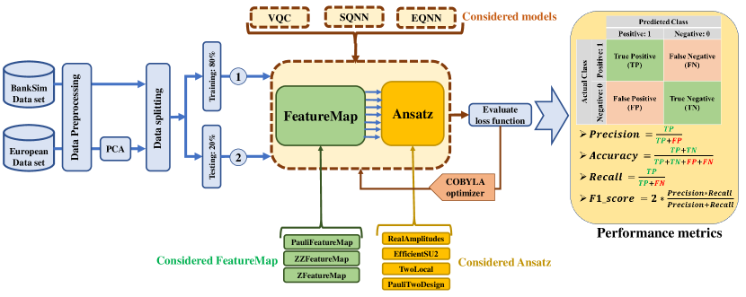
Figure 1: Overview of the proposed methodology. Two benchmark datasets undergo initial preprocessing, after which three QML models are evaluated. Each model is tested with three distinct feature map architectures, and each selected feature map is further assessed using four different ansatz configurations

The rest of the paper is structured as follows. In Sec. II, we review the existing literature on classical and QML approaches to financial fraud detection. In Sec. III, we provide the background and the architecture of different feature map and ansatz architectures. In Sec. IV, we describe the QML models employed and the associated circuit constructs. In Sec. V, we present the datasets used, report our experimental results, and highlight the model configurations achieving the highest performance. Finally, in Sec. VI, we conclude by summarizing our findings and discussing potential directions for future work.

II Literature Review

Classical ML algorithms have been extensively explored for detecting fraudulent credit card transactions. A variety of models, including multivariate logistic regression [19], support vector machines [20], and random forest classifiers [21, 22], have demonstrated varying degrees of success. More sophisticated approaches integrate intelligent techniques, such as optimized light gradient boosting machine [23], as well as deep learning architectures like auto-encoders and restricted Boltzmann machines [24], and graphical neural networks [25].

Despite significant progress in classical approaches, these methods face persistent challenges due to the volume, complexity, and continuously evolving patterns of fraudulent activities. This has motivated interest in QML, which employs quantum properties—including entanglement and superposition—to operate efficiently in high-dimensional feature spaces. As a result, QML has the potential to process large datasets more rapidly, capture complex interactions among transactional features, and express intricate patterns, offering tangible benefits for fraud detection tasks [26, 27, 28].

The emergence of accessible QML tools, such as IBM’s Qiskit and Xanadu’s PennyLane [29, 30], has further accelerated research in this area. Several studies have begun to explore QML solutions for fraud detection. For instance, Liang et al. introduced two quantum anomaly detection algorithms grounded in density estimation and multivariate Gaussian distributions that can be applied to fraudulent transaction identification [31]. A quantum graph convolutional neural network proposed expanded quantum neural network to graph-structured data [32], holding promise for fraud scenarios involving complex relational information. Another study compared quantum kernel-based anomaly detection with classical baselines such as one-class support vector machines, demonstrating the potential of QML in improving detection performance [33].

Additional research has directly compared quantum-enhanced methods to classical benchmarks. Grossi et al. evaluated a quantum support vector machine against traditional models like XGBoost and random forests within a financial fraud detection setting [34], while Shetakis et al. assessed quantum classifiers alongside classical artificial neural networks in a hybrid framework [35]. Explorations into more specialized QML architectures include investigations of quantum neural networks for graph-structured quantum data in Noisy Intermediate-Scale Quantum (NISQ) devices [36]. Recently, Quantum Graph Neural Networks (QGNN) have been employed to detect financial fraud, showcasing improvements over their classical GNN counterparts [37].

Beyond algorithmic innovations, hybrid frameworks have emerged; Innan et al. integrated QML with federated learning to propose quantum federated artificial neural networks for financial fraud detection [38], improving both privacy and detection effectiveness. Furthermore, Huot et al. introduced a QML model based on quantum auto-encoders for fraud detection [39], illustrating the adaptability of QML to various architectural paradigms. In summary, the literature demonstrates the potential of QML in enhancing credit card fraud detection. Quantum methods improve detection rates and reduce false positives, offering more robust protection for consumers and financial institutions. As research progresses, refining and optimizing QML architectures will be crucial, ensuring these emergent techniques can reliably outperform their classical counterparts and contribute to safer financial ecosystems.

III Background

The functionality of a QML model, as illustrated in Fig. 2, is based on an architecture that comprises three fundamental components. Initially, the feature map encodes the input features of the dataset, denoted as ${|\psi_{i}\rangle}_{i=1}^{n}$, using an encoding scheme $\Phi:x\rightarrow|\psi\rangle$. Subsequently, the ansatz $\mathbf{U}(\theta)$ applies trainable parameters $\theta$ through a sequence of quantum gates, evolving the quantum states of the system. The final component involves measurement and optimization, where the evolved quantum states are measured to extract quantum information. This information is then processed by a classical optimization algorithm, which iteratively adjusts the parameters $\theta$ to minimize the loss function, thereby enhancing the QML model’s performance. This optimization loop effectively bridges the quantum and classical domains, ensuring continuous refinement of the model’s predictive accuracy. Additionally, Fig. 3 shows the quantum gates commonly employed in the quantum circuits of QML models, highlighting their role in manipulating quantum states to perform the necessary computations for learning and optimization tasks.

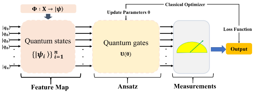
Figure 2: Fundamental architecture of a QML model. It begins with the transformation of classical data into quantum states, represented as $|\psi_{i}\rangle$. These states are processed by an ansatz $\mathbf{U}(\theta)$, which applies quantum gates such as rotation and entanglement. The model incorporates a classical optimizer that iteratively updates the parameters of the ansatz based on a loss function until convergence is achieved. Finally, the output of the ansatz is measured to provide the model’s predictions for various tasks.

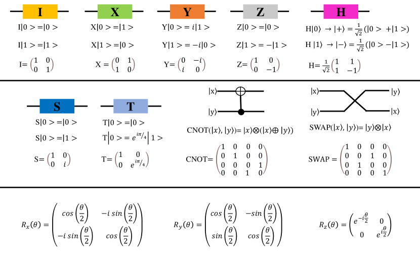
Figure 3: Graphical representation and mathematical expressions of selected single and two-qubit quantum gates.

III-A Features Maps

A quantum feature map encodes the classical input vector $\vec{x}$ into a quantum state $|\psi(\vec{x})\rangle$ in a Hilbert space $F$ through the mapping $x\mapsto|\psi(\vec{x})\rangle$. This feature map, also known as the unitary operator $U_{\psi}(\vec{x})$, generates the quantum state as ${|\psi(\vec{x})\rangle=U_{\psi}(\vec{x})|0\rangle}$. It acts on the ground or vacuum state $|0\rangle=|00\ldots 0\rangle$ of the Hilbert space $F$. Using this approach, the feature space becomes more complex, enabling a quantum classification system to identify intricate patterns in the input data [40]. Various types of feature maps exist; we focus on angle encoding, specifically the Pauli, ZZ, and Z feature maps.

III-A1 Pauli Feature Map

The Pauli feature map represents a quantum circuit that enables a Pauli expansion of a given dataset. The Pauli expansion is a method for representing the dataset as a product of Pauli operators, where each Pauli operator corresponds to a distinct feature within the data. The expression for the combination of Pauli operators is described as follows:

$$U_{\varphi_{s}(\vec{x})}=\exp\left(i\sum_{S\subseteq[n]}\varphi_{s}(\vec{x})\prod_{i\in S}P_{i}\right),$$ (1)

where $i$ is the set of qubit indices describing the connections in the feature map, $P_{i}\in\{I,X,Y,Z\}$ denotes the Pauli matrices, and $S$ describes the correlation between different qubits. The set $S$ belongs to the set of all combinations $S\in\left\{\binom{n}{k},\;k=1,\dots,n\right\}$. The term $\varphi_{s}(\vec{x})$ represents the data mapping function [41].

The data mapping function, $\varphi_{s}(\vec{x})$, maps classical input data $\vec{x}$ into the quantum circuit, enhancing the circuit’s representational capabilities. It is defined as follows:

$$\varphi_{s}(x)=\begin{cases}x_{0}&\text{si }s=\{i\}\\ \prod_{j\in S}(\pi-x_{j})&\text{si }|S|>1\end{cases}.$$ (2)

The Pauli feature map circuit is constructed by initially applying Hadamard gates to all qubits. Subsequently, a series of rotation gates are applied to the qubits, with the rotation angle of each qubit determined by the data mapping function $\varphi_{s}(\vec{x})$. Finally, entangling gates are applied to the qubits.

III-A2 ZZ Feature Map

The ZZ feature map is a specific implementation of the Pauli-Z operator. Representing a second-order Pauli-Z evolution, the ZZ operator is defined as:

$$ZZ=\begin{pmatrix}1&0\\ 0&-1\end{pmatrix}\otimes\begin{pmatrix}1&0\\ 0&-1\end{pmatrix}=\begin{pmatrix}1&0&0&0\\ 0&-1&0&0\\ 0&0&-1&0\\ 0&0&0&1\end{pmatrix},$$ (3)

which captures pairwise correlations between qubits. The circuit begins with Hadamard gates applied to all qubits, followed by a sequence of rotation and entanglement blocks. The rotation block utilizes a classical non-linear function, $\varphi(x)$, to determine rotation angles based on the input data; in this case, for example, seven features can be described as follows:

$$\varphi(x_{0},x_{1},\ldots,x_{6})=\prod_{i=0}^{6}(\pi-x_{i}).$$ (4)

Entanglement blocks are constructed using CNOT gates that entangle qubits according to a predefined structure. Repeated layers of rotation and entanglement blocks allow the circuit to encode increasingly complex correlations. The feature dimension corresponds to the number of qubits, and the repetition criterion determines the number of layers applied, making the ZZ feature map adaptable to the input data’s dimensionality and the desired circuit depth.

III-A3 Z Feature Map

The Z feature map class represents a first-order Pauli-Z evolution circuit. As it is a type of Pauli feature map and operates with fixed “Z” Pauli chains, its first-order expansion does not contain entangled gates. This feature map is especially well-suited to certain applications where a shallow, entanglement-free quantum circuit is required because of this special feature. Similar to the ZZ feature map, the Z feature map is customized to fit a specific number of qubits, known as the feature dimension, and allows the user to choose how many times the rotation blocks should be replicated. The circuit is built by applying Hadamard gates to each qubit, then rotation blocks. The rotation blocks are structured using the same methods used in the ZZ feature map.

The Z feature map encoding method also offers parameters like entity size, repetition count, and entanglement approach crucial for circuit inspection. Since there are no entanglement gates in the Z feature map, the entanglement strategy is zero. By offering a different quantum feature map that fits particular usage scenarios where entangled gates must be avoided, this feature map enhances the ZZ feature map method.

III-B Ansatz

An ansatz refers to a parameterized quantum circuit designed to approximate a solution to a specific problem or encode a given dataset into quantum states. It consists of a sequence of quantum gates with tunable parameters, enabling the circuit to explore various quantum states. By adjusting these parameters, the ansatz can be optimized to minimize a cost function or represent features of a given problem. The design of an ansatz is crucial in QML, as it determines the expressiveness and trainability of the model. Tailoring the ansatz to the specific problem can incorporate problem-relevant symmetries and constraints, improving efficiency and solution quality [42].

This study focuses on four distinct ansatz architectures: Real Amplitudes, Efficient SU2, Two Local, and Pauli Two Design. These architectures are chosen for their diverse properties and capabilities in capturing correlations and representing quantum states, as illustrated in Fig. 4.

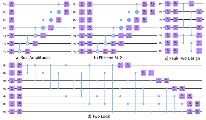
Figure 4: Architectures of the four ansatz variants utilized in this study, demonstrated on seven qubits: a) Real Amplitudes, b) Efficient SU2, c) Two Local, and d) Pauli Two Design, highlighting their structural differences and configurations.

III-B1 Real Amplitudes

The Real Amplitudes circuit serves as a heuristic test wave function. It comprises alternating layers of CNOT entanglement gates and $Y$-rotation gates, as illustrated in Fig. 4-a. The entanglement pattern can be pre-selected from standard configurations or customized by the user. Notably, the quantum states generated by this circuit have exclusively real amplitudes, with zero complex components, giving the circuit its name.

III-B2 Efficient SU2

The Efficient SU2 circuit consists of alternating layers of single-qubit $\mathrm{SU}(2)$ gates and CNOT entanglement gates, as shown in Fig. 4-b. The $\mathrm{SU}(2)$ group encompasses $2\times 2$ unitary matrices with a determinant of 1, such as Pauli rotation gates.

III-B3 Pauli Two Design

The Pauli Two Design circuit begins with an initial layer of gates, $\sqrt{H}=\mathbf{R}_{y}\left(\frac{\pi}{4}\right)$, followed by alternating layers of single-qubit rotation gates and entanglement gates, as shown in Fig. 4-c. In the rotation layers, single-qubit Pauli rotations are applied along axes $X$, $Y$, or $Z$, selected uniformly at random. The entanglement layers consist of controlled-Z (CZ) gates arranged in a matching pattern.

III-B4 Two Local

The Two Local circuit is a parametric quantum circuit composed of alternating rotation and entanglement layers. The rotation layers apply single-qubit gates to all qubits, while the entanglement layers employ two-qubit gates to establish entanglement according to a predefined strategy, as represented in Fig. 4-d. The specific rotation and entanglement gates can be defined explicitly, such as $R_{Y}$ and CNOT.

IV QML Models

IV-A Variational Quantum Classifiers

The VQC is a parameterized quantum circuit whose parameters, referred to as learnable weights, are optimized using classical methods to minimize a loss function. The operation of a VQC, as shown in Fig. 5, proceeds as follows: First, the quantum state preparation step initializes the circuit with parameters $\boldsymbol{\theta}=\left(\theta_{1},\theta_{2},\dots,\theta_{n}\right)$, where $n$ is the number of registers in the circuit. These parameters represent the learnable weights, which are initially set to random values in the range $0\leq\theta_{i}\leq 1$. The initial quantum state denoted as $\left|\Psi_{0}(\theta)\right\rangle$, typically consists of simple quantum states, such as a tensor product of $\left|0\right\rangle$ states.

Next, a unitary transformation is applied. This step involves the application of a sequence of quantum gates to the initial state. Let $G_{i}\in\left\{I,X,Y,Z,H,S,T,\mathrm{R}_{X},\mathrm{R}_{Y},\mathrm{R}_{Z},\mathrm{CNOT},\mathrm{SWAP},\dots\right\}$ represent the set of possible quantum gates, where $1\leq i\leq m$. The gates are applied to form a unitary operator $U=\bigotimes_{i=1}^{m}G_{i}$. The resulting quantum state after the unitary transformation is given by:

$$U\left|\Psi_{0}(\theta)\right\rangle=\left|\Psi(\theta)\right\rangle.$$ (5)

Finally, measurement is performed on the transformed quantum state $\left|\Psi(\theta)\right\rangle$ to extract information and compute a classical output. Steps 2 and 3 are iteratively executed to minimize the loss function $J(\theta)$. The process terminates when an acceptance criterion, such as convergence of the loss function, is met [43].

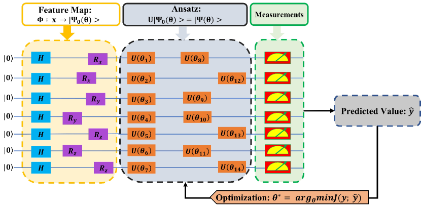
Figure 5: Architecture of the VQC model, it consists of a feature map, the $U$ operator is then applied in a measurement to obtain the classical output $\hat{y}$. This process is repeated where a classical optimizer is applied to update the parameters $\theta$ until the loss function $J(y;\hat{y})$ is minimized.

IV-B Estimator Quantum Neural Networks

The EQNN is a hybrid architecture that integrates classical and QNNs. As shown in Fig. 6, the EQNN is composed of three primary components: a quantum feature map, an ansatz including the measurement, and a classical neural network.

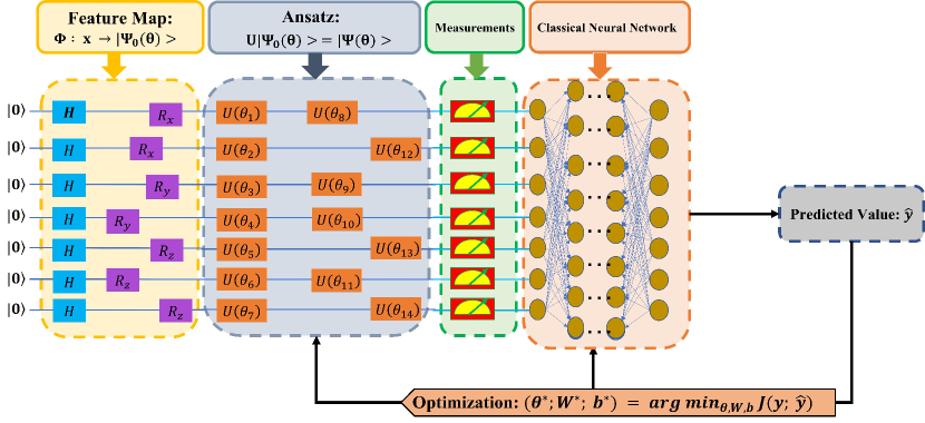
Figure 6: Architecture of the EQNN model. The process starts with a feature map, followed by an ansatz and measurements to extract classical data. This data is then passed through a fully connected classical neural network, which computes the output value $\hat{y}$. A classical optimizer iteratively updates the parameters $\theta^{*}$, $\mathbf{W}^{*}$, and $b^{*}$ to minimize the loss function $J(y,\hat{y})$.

The operation of the EQNN begins with data preparation via a quantum feature map. Classical data, denoted as $\mathbf{x}=(x_{1},x_{2},\dotsc,x_{n})$, is encoded into quantum states $\left|\Psi_{0}(\theta)\right\rangle$ through the quantum feature map $\Phi:\mathbf{x}\mapsto\left|\Psi_{0}(\theta)\right\rangle$. Following the encoding stage, the quantum states $\left|\Phi(\mathbf{x})\right\rangle$ are processed through the ansatz to transform the encoded states into output quantum states $\left|\Psi(\theta)\right\rangle$. Subsequently, measurements are performed on the output states $\left|\Psi(\theta)\right\rangle$, extracting classical features from the quantum system. These features are obtained by measuring the qubits in the computational basis ${\left|0\right\rangle,\left|1\right\rangle}$. The classical features obtained from the measurement stage are then processed by a fully connected classical neural network, which computes the output values $\hat{y}$. This step combines the strengths of classical and quantum processing for robust learning. Finally, the model undergoes an optimization phase where the parameters of both the quantum and classical components are adjusted. The goal is to determine the optimal parameters $\theta^{*}$ for the ansatz and the weights $\mathbf{W}^{*}$ and biases $b^{*}$ of the classical neural network by minimizing the loss function $J(y;\hat{y})$. This process can be formulated as:

$$(\theta^{*};\mathbf{W}^{*};b^{*})=\arg\min_{\theta,\mathbf{W},b}J(y;\hat{y}).$$ (6)

The optimization of quantum and classical parameters is conducted simultaneously, ensuring efficient learning and improved performance.

IV-C Sampler Quantum Neural Networks

The SQNN, similar to the EQNN, also features a hybrid classical-quantum architecture. However, the key distinction of the SQNN lies in the inclusion of a quantum sampler, which extracts examples of quantum states based on the complex probability distribution associated with these states, as shown in Fig. 7.

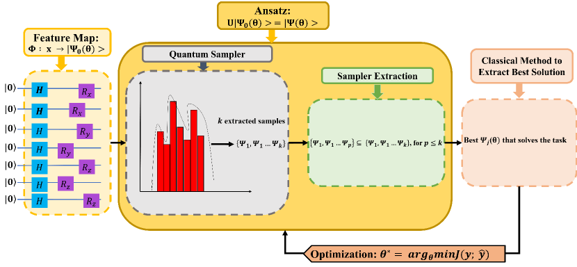
Figure 7: Architecture of the SQNN model. It consists of a feature map and an ansatz that incorporates a quantum sampler, followed by the extraction of samples generated by the quantum sampler.

The SQNN operates through several stages. First, the process begins with the generation of quantum states via a feature map identical to the first step in the EQNN model. Next, a quantum sampler is applied. This step aims to efficiently extract examples of quantum states corresponding to the complex probability distribution of the problem’s solution in a specific variable configuration.

Following this, samples are extracted from the examples generated by the quantum sampler. The extracted samples are then processed using classical methods to identify the best solutions, where the optimal solutions for the given task are selected using a classical optimization scheme. Finally, a classical optimization method is employed to find the optimal parameters by minimizing the loss function, expressed as:

$$\theta^{*}=\arg\min_{\theta}J(y,\hat{y}),$$ (7)

where the optimized $\theta$ values are returned to the quantum circuit. The entire process is repeated iteratively until the optimal parameter values are determined, ensuring the model’s convergence to the best solutions for the given problem.

V Results and Discussion

V-A Dataset and Feature Selection

The first dataset used in this study is derived from BankSim [44], an agent-based bank payment simulator based on aggregated transactional data provided by a leading bank in Spain. BankSim is designed to generate synthetic data tailored for fraud detection research. To achieve this, statistical analysis and social network analysis are utilized to study relationships between merchants and customers, resulting in a calibrated model [45].

The BankSim dataset comprises 594,643 records obtained over 180 simulation steps, equivalent to approximately six months of activity. Of these records, 587,443 are regular payments, while 7,200 represent fraudulent transactions. The simulated frauds are introduced by modeling thieves stealing an average of three cards per stage and conducting around two fraudulent transactions per day. This dataset includes nine feature columns and one target column, which are essential for analyzing patterns and characteristics. The features are as follows:

• “Step”: Represents the time aspect, designating the simulation day, spanning 180 steps over six months.

• “Customer”: Identifies individual customers involved in transactions.

• “ZipCodeOrigin”: Indicates the origin postcode of each transaction, facilitating geographical analysis.

• “Merchant”: Identifies merchants involved in transactions.

• “ZipMerchant”: Provides the postcode associated with each merchant.

• “Age”: Categorizes customer age into bands: ’0’ ($\leq 18$), ’1’ (19–25), ’2’ (26–35), ’3’ (36–45), ’4’ (46–55), ’5’ (56–65), ’6’ ($>65$), and ’U’ (Unknown).

• “Gender”: Categorizes customers as “E” (Enterprise), “F” (Female), “M” (Male), or “U” (Unknown).

• “Category”: Captures the purchase category, indicating the type of transaction.

• “Amount”: Represents the monetary value of transactions.

• “Fraud”: The target variable, a binary class where 1 indicates fraud and 0 indicates non-fraud.

As part of preprocessing, inconsistencies in the “Age” column are resolved by converting categorical values into integers using regular expressions. Categorical features such as “Customer”, “Gender”, “Merchant”, and “Category” are numerically encoded for efficient model training. Additionally, the features “ZipCodeOrigin” and “ZipMerchant” are removed due to their lack of variability, and the remaining features are converted into numerical values to ensure data consistency.

The second dataset is a publicly available credit card fraud detection dataset [46], containing European cardholder transactions. Features are derived using Principal Component Analysis (PCA) on real user data. Each transaction is labeled as fraud (1) or non-fraud (0), with 28 PCA-transformed features, as well as “Time” and “Amount”.

• “Time”: Indicates the elapsed time (in seconds) between transactions.

• “Amount”: Represents the monetary value of transactions.

• “Class”: The target variable, where 1 indicates fraud and 0 indicates non-fraud.

This dataset is unbalanced, containing 492 fraud cases out of 284,807 transactions, with the positive class representing only 0.172% of all transactions. To address the class imbalance in both datasets, “Random Under Sampling” was implemented to create balanced datasets with a 50/50 ratio. Each dataset was reduced to 492 fraudulent and 492 non-fraudulent transactions. PCA was applied to the European dataset, reducing its dimensions to seven features named “V1” through “V7”.

With the datasets balanced and preprocessed, visualizations are generated to understand feature relationships and their importance. Figs 8 and 9 illustrate the correlation matrices, highlighting key interactions. For instance, in the BankSim dataset, “Category” has a strong negative correlation with “Fraud”, while “Merchant” and “Amount” exhibit positive correlations. In the European dataset, features such as “V1” and “V2” show significant correlations with “Class”.

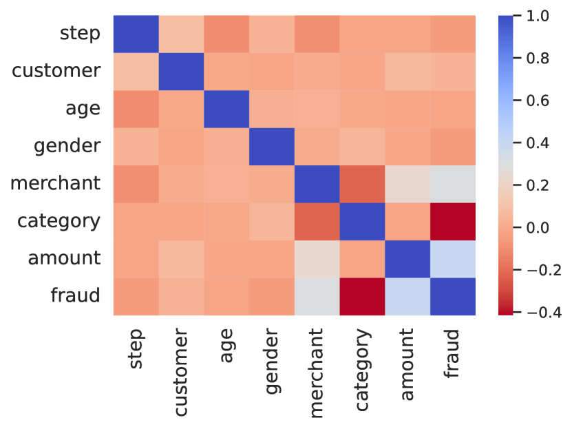
Figure 8: Correlation matrix of the BankSim dataset. Features such as “Category” show a strong negative correlation with the label “Fraud”, while “Merchant” and “Amount” have positive correlations, indicating their importance in fraud detection.

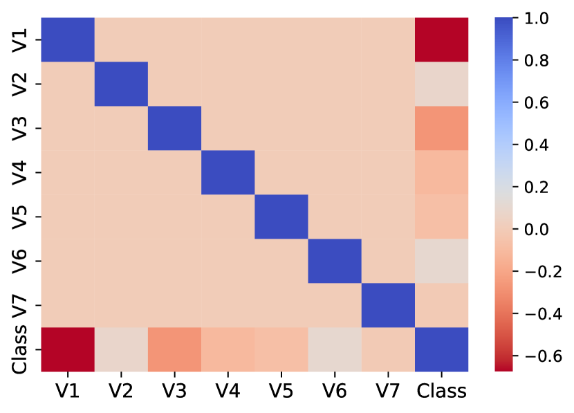
Figure 9: Correlation matrix of the European dataset. “V1” has a strong negative correlation with “Class”, while “V2” and “V6” show moderate positive correlations, suggesting their relevance for fraud detection.

As shown in Figs. 10 and 11, the analysis identifies specific features as particularly influential for predicting fraud. This insight allows us to focus on these key features to enhance the model’s performance and accuracy.

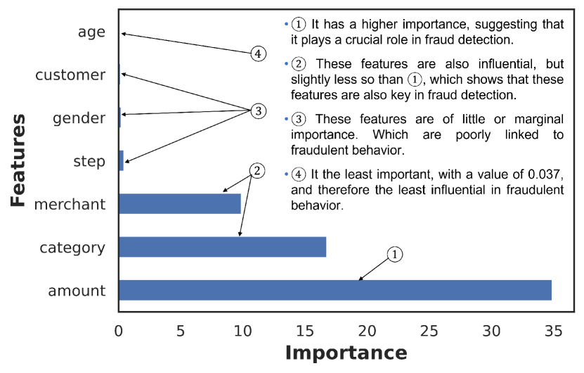
Figure 10: Feature importance for the BankSim dataset. “Amount”, “Category”, and “Merchant” are critical for fraud detection, while “Step”, “Gender”, and “Age” have minimal influence.

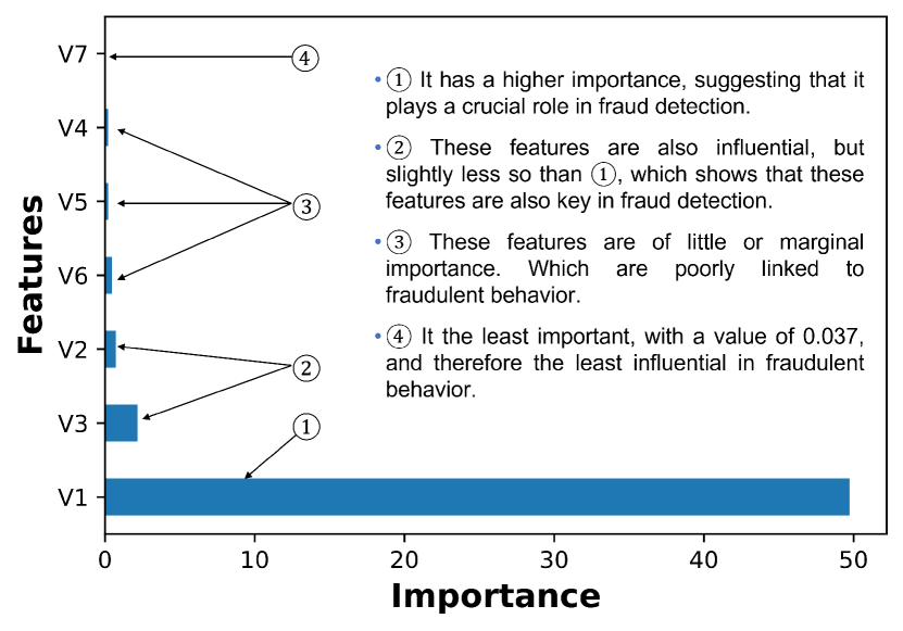
Figure 11: Feature importance for the European dataset. “V1” and “V3” are the most influential features for fraud prediction, with minimal contributions from other variables.

V-B Experimental Setup

To ensure the reliability of the fraud detection analysis, a comprehensive data preparation process is conducted to confirm the datasets’ quality and suitability for training and evaluating robust models. The datasets are split into 80% training and 20% testing subsets. The training set denoted as $X_{\text{train}}$ and $y_{\text{train}}$, is used to train the models, while the testing set, represented by $X_{\text{test}}$ and $y_{\text{test}}$, remains unseen during training and is used to evaluate model performance.

For each dataset, the feature matrix $X$ includes all relevant features except the label column, which serves as the target variable $y$. The target variable distinguishes between fraudulent transactions (coded as “1”) and non-fraudulent transactions (coded as “0”), enabling the models to learn patterns and accurately classify new data. To normalize the feature values and enhance model stability, scikit-learn’s MinMaxScaler is employed, scaling all feature values to the range [0, 1] without altering their distribution. Each QML model is tested under identical configurations, with three feature map architectures and four ansatz architectures, resulting in twelve unique configurations per model. The analysis is carried out on two datasets.

Model optimization is handled using Qiskit’s COBYLA optimizer, chosen for its efficiency and ability to converge to optimal solutions effectively. The Aer backend with the QasmSimulator is utilized to simulate quantum circuits, ensuring a seamless and transparent training process. Following training, the models’ performance is meticulously evaluated using key metrics, including accuracy, precision, recall, F1-score, and loss.

The hyperparameters and configurations used in this study are summarized in Table I. These configurations are carefully selected to ensure an optimal balance between computational efficiency and model performance.

TABLE I: Configuration and hyperparameters used.

Parameter	Value
Number of Qubits	4, 6, 7
Optimizer	COBYLA, ADAM, Gradient Descent
Maximum Iterations	350
Test Set Size	20%
Performance Metrics	Accuracy, Precision, Recall, F1-score, Loss
Repetition of Feature Map	1, 2
Repetition of Ansatz	1, 2
Libraries and Backend	Qiskit, QasmSimulator

V-C BankSim Dataset

Table II highlights the performance of the VQC model. Notably, the ZZ and Pauli feature maps paired with the Efficient SU2 ansatz yield the highest F1-scores of 0.68 and 0.71, respectively. These results suggest that introducing entanglement through the feature map improves the VQC’s ability to learn complex interactions. Fig. 12 supports this, as most configurations stabilize after oscillatory dynamics, indicating successful optimization. Similarly, Table III reveals the robust performance of the SQNN model. The Pauli feature map combined with Two Local and Real Amplitudes achieves F1-scores of 0.84 and 0.85, respectively, showcasing the effectiveness of these configurations. Fig. 13 demonstrates consistent convergence behavior across these configurations, with some achieving minimal loss values after initial oscillations. In contrast, Table IV shows that the EQNN model generally underperforms compared to VQC and SQNN. While the Pauli feature map with Pauli Two Design achieves a peak F1-score of 0.59, configurations involving the Z feature map yield significantly lower scores, underscoring the importance of entanglement in feature maps. Fig. 17 corroborates these findings, representing varying levels of convergence stability across configurations.

TABLE II: Performance metrics of the VQC model on the BankSim dataset.

Model	Feature Map	Ansatz	Accuracy	Precision	Recall	F1_score
	Z	Real Amplitudes	0.52	0.48	0.8	0.6
		Two Local	0.54	0.5	0.84	0.62
		Efficient SU2	0.65	0.68	0.44	0.54
		Pauli Two Design	0.55	0.51	0.51	0.51
VQC	ZZ	Real Amplitudes	0.74	0.75	0.62	0.68
		Two Local	0.65	0.62	0.6	0.61
		Efficient SU2	0.76	0.85	0.56	0.68
		Pauli Two Design	0.51	0.46	0.42	0.44
	Pauli	Real Amplitudes	0.73	0.69	0.72	0.7
		Two Local	0.73	0.69	0.72	0.71
		Efficient SU2	0.76	0.85	0.56	0.68
		Pauli Two Design	0.5	0.45	0.46	0.46

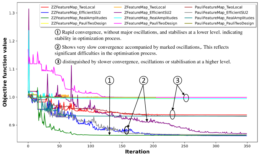
Figure 12: VQC loss function on the BankSim dataset. Most configurations demonstrate stabilization over time, indicating consistent optimization behavior. However, some configurations exhibit a zigzag pattern during convergence, reflecting oscillatory dynamics before eventual stabilization.

TABLE III: Performance metrics of the SQNN model on the BankSim dataset.

Model	Feature Map	Ansatz	Accuracy	Precision	Recall	F1_score
	Z	Real Amplitudes	0.86	0.82	0.88	0.85
		Two Local	0.73	0.75	0.58	0.66
		Efficient SU2	0.83	0.81	0.82	0.81
		Pauli Two Design	0.85	0.78	0.91	0.84
SQNN	ZZ	Real Amplitudes	0.74	0.77	0.61	0.68
		Two Local	0.83	0.85	0.76	0.8
		Efficient SU2	0.77	0.73	0.76	0.75
		Pauli Two Design	0.64	0.63	0.51	0.56
	Pauli	Real Amplitudes	0.82	0.82	0.76	0.79
		Two Local	0.86	0.84	0.84	0.84
		Efficient SU2	0.77	0.81	0.64	0.72
		Pauli Two Design	0.64	0.59	0.7	0.64

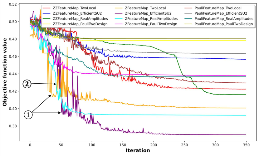
Figure 13: SQNN loss function on the BankSim dataset. The configuration in \raisebox{-0.9pt}{1}⃝ achieves convergence with minimal loss but does not correspond to the absolute minimum loss. Configurations labeled as \raisebox{-0.9pt}{2}⃝ exhibit similar behaviors across different levels of loss, characterized by a zigzag pattern during the initial optimization phase, eventually stabilizing after requiring more iterations to converge.

TABLE IV: Performance metrics of the EQNN model on the BankSim dataset.

Model	Feature Map	Ansatz	Accuracy	Precision	Recall	F1_score
	Z	Real Amplitudes	0.45	0.22	0.49	0.31
		Two Local	0.46	0.22	0.50	0.31
		Efficient SU2	0.46	0.22	0.50	0.31
		Pauli Two Design	0.32	0.28	0.34	0.28
EQNN	ZZ	Real Amplitudes	0.45	0.46	0.48	0.37
		Two Local	0.50	0.57	0.53	0.42
		Efficient SU2	0.53	0.60	0.56	0.49
		Pauli Two Design	0.51	0.52	0.52	0.50
	Pauli	Real Amplitudes	0.47	0.49	0.49	0.41
		Two Local	0.55	0.63	0.58	0.51
		Efficient SU2	0.52	0.53	0.52	0.51
		Pauli Two Design	0.60	0.61	0.61	0.59

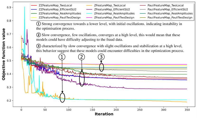
Figure 14: EQNN loss function on the BankSim dataset. Most configurations demonstrate steady convergence, stabilizing after a period of oscillations and reaching varying levels of loss. While some achieve minimal loss, others stabilize at higher values, reflecting differences in optimization effectiveness.

V-C1 Analysis of Feature Maps

Feature maps play a crucial role in capturing complex data patterns. The Z feature map, while computationally efficient, lacks expressivity due to the absence of entanglement. This limitation is evident in the EQNN model’s F1-scores, which stagnate at 0.31 across most ansatz configurations (Table IV). Conversely, the ZZ feature map introduces pairwise entanglement, significantly enhancing performance for VQC and SQNN. For instance, the ZZ feature map paired with Efficient SU2 achieves F1-scores of 0.68 and 0.75 for VQC and SQNN, respectively. The Pauli feature map emerges as the most robust, consistently delivering superior results across all models. In SQNN, its configuration with Two Local achieves the highest F1-score of 0.84, as shown in Table III. For EQNN, the Pauli feature map compensates for architectural limitations, achieving a peak F1-score of 0.59 with Pauli Two Design. These findings emphasize that feature maps incorporating entanglement, such as ZZ and Pauli, enhance model performance, especially when paired with expressive ansatz configurations.

V-C2 Analysis of Ansatz

The choice of ansatz significantly impacts the quantum circuit’s ability to model complex functions. Real Amplitudes, with its simple configuration, performs competitively in SQNN, achieving an F1-score of 0.85 with the Z feature map (Table III). However, it struggles to capture intricate interactions in EQNN, resulting in suboptimal performance.

Two Local, characterized by alternating single-qubit rotations and entangling gates, exhibits strong performance in SQNN (F1-score of 0.84 with the Pauli feature map). However, its performance in EQNN remains moderate, likely due to limited parametrization. Efficient SU2 emerges as the most versatile ansatz, achieving consistently strong metrics across models. Notably, it delivers F1-scores of 0.68 and 0.81 for VQC and SQNN, respectively, when paired with ZZ and Z feature maps.

In contrast, Pauli Two Design shows inconsistent results. While it achieves its best performance in EQNN with the Pauli feature map (F1-score of 0.59), its performance across other configurations varies significantly. This underscores the need to carefully align ansatz configurations with the chosen feature map and model architecture to maximize performance.

V-D European Dataset

The VQC model’s results, as presented in Table V, show that the configuration of the Z feature map with the Pauli Two Design ansatz achieves the highest F1-score of 0.88. Similarly, the ZZ and Pauli feature maps paired with Two Local yield strong F1-scores of 0.83 each, indicating the robustness of Two Local across feature maps. Fig. 15 further supports these findings, highlighting configurations with steady convergence and minimal loss. Table VI demonstrates that SQNN achieves its best performance when the Z feature map is paired with the Two Local ansatz (F1-score of 0.80). The configuration of the Pauli feature map with the Two Local ansatz also performs well, achieving an F1-score of 0.81. These configurations exhibit consistent convergence behavior, as shown in Fig. 16. In contrast, other configurations either stabilize at higher loss values or demonstrate slower convergence. The EQNN model’s performance, as outlined in Table VII, generally lags behind VQC and SQNN. The best performance is achieved with the ZZ feature map and the Two Local ansatz, yielding an F1-score of 0.52. Fig. 17 illustrates the optimization dynamics, where most of these configurations exhibit oscillatory behavior before stabilizing at suboptimal loss values.

TABLE V: Performance metrics of the VQC model on the European dataset.

Model	Feature Map	Ansatz	Accuracy	Precision	Recall	F1_score
	Z	Real Amplitudes	0.7	1	0.34	0.51
		Two Local	0.88	1	0.73	0.84
		Efficient SU2	0.86	1	0.68	0.81
		Pauli Two Design	0.9	1	0.78	0.88
VQC	ZZ	Real Amplitudes	0.74	1	0.43	0.6
		Two Local	0.87	1	0.71	0.83
		Efficient SU2	0.78	0.94	0.55	0.69
		Pauli Two Design	0.73	0.77	0.56	0.65
	Pauli	Real Amplitudes	0.74	1	0.43	0.6
		Two Local	0.87	1	0.71	0.83
		Efficient SU2	0.78	0.94	0.55	0.69
		Pauli Two Design	0.81	0.96	0.6	0.73

Figure 15: VQC loss function on the European dataset. The configuration in \raisebox{-0.9pt}{4}⃝ demonstrates fast convergence with minimal loss, showing some oscillations during the first 50 iterations before stabilizing. The configurations in \raisebox{-0.9pt}{5}⃝ exhibit similar behavior, converging steadily over 200 iterations to achieve relatively low loss values. In contrast, the configurations in \raisebox{-0.9pt}{6}⃝ converge more rapidly but stabilize at a higher loss value, indicating suboptimal performance.

TABLE VI: Performance metrics of the SQNN model on the European dataset.

Model	Feature Map	Ansatz	Accuracy	Precision	Recall	F1_score
	Z	Real Amplitudes	0.64	1	0.21	0.34
		Two Local	0.85	1	0.67	0.8
		Efficient SU2	0.8	1	0.56	0.72
		Pauli Two Design	0.75	1	0.45	0.62
SQNN	ZZ	Real Amplitudes	0.65	1	0.23	0.37
		Two Local	0.86	1	0.68	0.68
		Efficient SU2	0.8	1	0.56	0.72
		Pauli Two Design	0.69	0.89	0.36	0.51
	Pauli	Real Amplitudes	0.65	1	0.23	0.37
		Two Local	0.86	1	0.68	0.81
		Efficient SU2	0.8	1	0.56	0.72
		Pauli Two Design	0.8	0.94	0.6	0.73

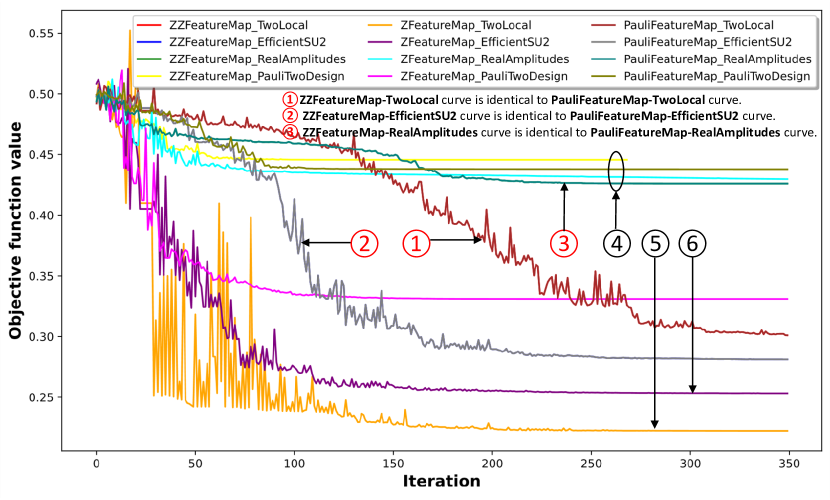
Figure 16: SQNN loss function on the European dataset. The configurations highlighted in \raisebox{-0.9pt}{4}⃝ demonstrate faster convergence but do not reach the lowest loss value. The configuration in \raisebox{-0.9pt}{5}⃝ converges quickly and achieves the minimum loss among all configurations, making it the most favorable. In contrast, the configuration marked as \raisebox{-0.9pt}{6}⃝ stabilizes first but achieves a medium loss value compared to the others, indicating limited performance.

TABLE VII: EQNN model performance metrics of the SQNN model on the European dataset.

Model	Feature Map	Ansatz	Accuracy	Precision	Recall	F1_score
	Z	Real Amplitudes	0.45	0.22	0.50	0.31
		Two Local	0.49	0.73	0.52	0.37
		Efficient SU2	0.46	0.22	0.5	0.31
		Pauli Two Design	0.41	0.21	0.45	0.29
EQNN	ZZ	Real Amplitudes	0.45	0.45	0.47	0.40
		Two Local	0.55	0.61	0.57	0.52
		Efficient SU2	0.45	0.45	0.47	0.41
		Pauli Two Design	0.44	0.43	0.46	0.39
	Pauli	Real Amplitudes	0.45	0.45	0.47	0.40
		Two Local	0.55	0.61	0.57	0.52
		Efficient SU2	0.45	0.45	0.47	0.41
		Pauli Two Design	0.47	0.48	0.48	0.44

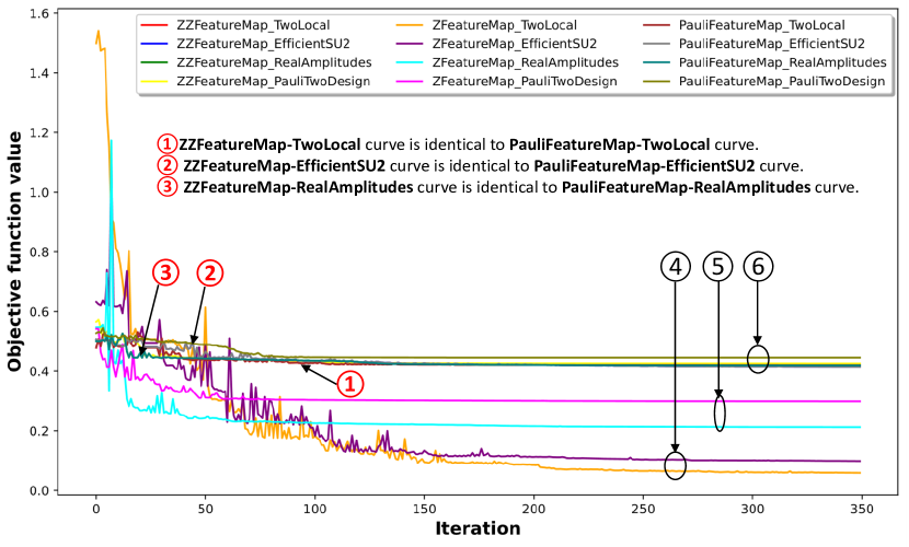
Figure 17: EQNN loss function on the European dataset. The configurations highlighted in \raisebox{-0.9pt}{4}⃝ exhibit slow convergence to the lowest loss value, accompanied by oscillatory behavior. In contrast, the configurations marked as \raisebox{-0.9pt}{5}⃝ demonstrate slower convergence and stabilize at a higher loss value, suggesting reduced effectiveness. Finally, the configurations labeled \raisebox{-0.9pt}{6}⃝ achieve faster convergence, indicating a more favorable performance among the analyzed configurations.

V-D1 Analysis of Feature Maps

The Z feature map consistently delivers strong results across models. For instance, in VQC, its configuration with the Pauli Two Design ansatz achieves the highest F1-score of 0.88 (Table V). Similarly, in SQNN, the Z feature map paired with the Two Local ansatz yields an F1-score of 0.80 (Table VI). However, the Z feature map’s performance in EQNN is limited, with the highest F1-score being 0.52. The ZZ feature map introduces pairwise entanglement, leading to competitive results. In VQC, its configuration with the Two Local ansatz achieves an F1-score of 0.83. Similarly, in SQNN, the ZZ feature map paired with the Efficient SU2 ansatz results in an F1-score of 0.72. However, its performance in EQNN remains limited, with an F1-score of 0.52 when paired with the Two Local ansatz. The Pauli feature map demonstrates consistent performance across VQC and SQNN. In VQC, its configuration with the Two Local ansatz achieves an F1-score of 0.83, while in SQNN, the same configuration results in an F1-score of 0.81. However, in EQNN, its best performance remains low, with an F1-score of 0.52.

V-D2 Analysis of Ansatz

Real Amplitudes, while computationally efficient, struggle with complex interactions. For example, in VQC, it achieves an F1-score of 0.6 with the Pauli feature map, but its performance in SQNN and EQNN remains limited. Two Local emerges as the most robust ansatz, consistently delivering strong results across models. In VQC, it achieves F1-scores of 0.84 and 0.83 with the ZZ and Pauli feature maps, respectively. In SQNN, it attains an F1-score of 0.81 with the Pauli feature map. This versatility underscores its ability to effectively capture intricate data patterns when paired with expressive feature maps. Efficient SU2 shows strong performance in VQC, achieving an F1-score of 0.81 with the Z feature map. However, its performance in EQNN is moderate, likely due to insufficient parametrization. Pauli Two Design exhibits erratic outcomes. In VQC, it achieves an F1-score of 0.88 with the Z feature map, but its performance in SQNN and EQNN is inconsistent, with F1-scores of 0.73 and 0.44, respectively. This variability suggests that Pauli Two Design’s effectiveness is highly dependent on the model architecture and feature map used.

V-E Discussion

The analytical results highlight the critical interaction between feature maps, ansatz configurations, and dataset characteristics in shaping model performance. The ability of a model to balance the performance metrics is heavily influenced by the capacity of the feature map to encode meaningful data relationships and the ansatz to exploit these encoded patterns effectively. This interaction varies across datasets and model architectures, emphasizing the importance of a tailored approach to configuration selection. The performance variations across models reflect their inherent architectural differences. VQC consistently leverages expressive ansatz-feature map combinations to achieve high precision and balanced F1-scores, especially on the European dataset. SQNN demonstrates robust adaptability, excelling in configurations that pair computational efficiency with high representational power, such as the Z feature map with Real Amplitudes on the BankSim dataset. In contrast, EQNN’s limitations in handling complex patterns suggest that either its architectural simplicity or constraints in its quantum circuit design impede its ability to capitalize on the available data encodings. These disparities underscore the importance of aligning model architectures with feature map and ansatz choices to maximize performance.

Additionally, the results suggest that while entanglement-enhanced feature maps like ZZ and Pauli can add value, their success is contingent on the model’s ability to process the increased complexity. Models like SQNN benefit significantly from such feature maps when paired with flexible ansatzes like Two Local, which provide a rich search space to navigate complex data relationships. Conversely, simpler feature maps like Z demonstrate versatility and effectiveness, likely due to their ability to reduce computational noise and simplify optimization. This analysis underscores the necessity of a strategic, data-driven approach to selecting feature map-ansatz configurations. The interplay between dataset characteristics and model architecture determines the optimal balance between computational efficiency and performance, guiding the design of more effective quantum and hybrid quantum models for fraud detection.

VI Conclusion

This study provides an insightful comparison of the performance of VQC, SQNN, and EQNN models in the context of financial fraud detection, highlighting their unique capabilities and limitations. By systematically exploring the impact of feature maps and ansatz configurations across two diverse datasets, the analysis underscores the critical factors influencing the effectiveness of QML models. The results demonstrate that VQC and SQNN models are highly competitive in their ability to detect fraud, with VQC achieving the highest performance. In contrast, EQNN showed limited capacity to handle the complexity of the datasets, pointing to potential areas for architectural enhancement. The findings emphasize the significance of tailoring model configurations, including selecting feature maps and ansatzes, to align with specific data characteristics and performance requirements.

This work contributes to a deeper understanding of the interplay between quantum model design and application context, providing a foundation for optimizing QML models in financial fraud detection. Future research can build on these findings by exploring advanced quantum architectures and alternative configurations to further enhance the utility of QML in tackling fraud and other high-stakes classification problems.

References

- [1] J. Robinson and M. Edwards, “Fraudsters target the elderly: Behavioural evidence from randomised controlled scam-baiting experiments,” Security Journal, pp. 1–24, 2024.
- [2] S. Byrne and J. Byrne, “Scams, cons, frauds, and deceptions,” pp. 1185–1193, 2023.
- [3] E. B. Authority and E. C. Bank, “2024 report on payment fraud,” 2024. [Online]. Available: www.ecb.europa.eu/press/pr/date/2024/html/ecb.pr240801~f21cc4a009.en.html
- [4] T. Baabdullah, A. Alzahrani, D. B. Rawat, and C. Liu, “Efficiency of federated learning and blockchain in preserving privacy and enhancing the performance of credit card fraud detection (ccfd) systems,” Future Internet, vol. 16, no. 6, p. 196, 2024.
- [5] I. D. Mienye and N. Jere, “Deep learning for credit card fraud detection: A review of algorithms, challenges, and solutions,” IEEE Access, 2024.
- [6] M. Schuld, I. Sinayskiy, and F. Petruccione, “An introduction to quantum machine learning,” Contemporary Physics, vol. 56, no. 2, pp. 172–185, 2015.
- [7] S. Dutta, N. Innan, A. Marchisio, S. B. Yahia, and M. Shafique, “QADQN: Quantum attention deep q-network for financial market prediction,” arXiv preprint arXiv:2408.03088, 2024.
- [8] N. Innan, A. Marchisio, M. Bennai, and M. Shafique, “Lep-qnn: Loan eligibility prediction using quantum neural networks,” arXiv preprint arXiv:2412.03158, 2024.
- [9] S. Dutta, N. Innan, S. B. Yahia, and M. Shafique, “AQ-PINNs: Attention-enhanced quantum physics-informed neural networks for carbon-efficient climate modeling,” arXiv preprint arXiv:2409.01626, 2024.
- [10] I. Chen, N. Innan, S. K. Roy, and J. Saroni, “Crossing the gap using variational quantum eigensolver: A comparative study,” arXiv preprint arXiv:2405.11687, 2024.
- [11] N. Innan, M. A.-Z. Khan, and M. Bennai, “Quantum computing for electronic structure analysis: Ground state energy and molecular properties calculations,” Materials Today Communications, vol. 38, p. 107760, 2024.
- [12] W. E. Maouaki, N. Innan, A. Marchisio, T. Said, M. Bennai, and M. Shafique, “Quantum clustering for cybersecurity,” arXiv preprint arXiv:2408.02314, 2024.
- [13] P. Pathak, V. Oad, A. Prajapati, and N. Innan, “Resource allocation optimization in 5g networks using variational quantum regressor,” in 2024 International Conference on Quantum Communications, Networking, and Computing (QCNC). IEEE, 2024, pp. 101–105.
- [14] N. Innan, O. I. Siddiqui, S. Arora, T. Ghosh, Y. P. Koçak, D. Paragas, A. A. O. Galib, M. A.-Z. Khan, and M. Bennai, “Quantum state tomography using quantum machine learning,” Quantum Machine Intelligence, vol. 6, no. 1, p. 28, 2024.
- [15] N. Innan, M. A.-Z. Khan, B. Panda, and M. Bennai, “Enhancing quantum support vector machines through variational kernel training,” Quantum Information Processing, vol. 22, no. 10, p. 374, 2023.
- [16] N. Innan and M. Bennai, “A variational quantum perceptron with grover’s algorithm for efficient classification,” Physica Scripta, vol. 99, no. 5, p. 055120, 2024.
- [17] N. Innan, M. A.-Z. Khan, A. Marchisio, M. Shafique, and M. Bennai, “Fedqnn: Federated learning using quantum neural networks,” in 2024 International Joint Conference on Neural Networks (IJCNN), 2024, pp. 1–9.
- [18] N. Innan, M. A.-Z. Khan, and M. Bennai, “Financial fraud detection: a comparative study of quantum machine learning models,” International Journal of Quantum Information, vol. 22, no. 02, p. 2350044, 2024.
- [19] H. Z. Alenzi and N. O. Aljehane, “Fraud detection in credit cards using logistic regression,” International Journal of Advanced Computer Science and Applications, vol. 11, no. 12, 2020.
- [20] S. Kumar, V. K. Gunjan, M. D. Ansari, and R. Pathak, “Credit card fraud detection using support vector machine,” in Proceedings of the 2nd International Conference on Recent Trends in Machine Learning, IoT, Smart Cities and Applications: ICMISC 2021. Springer, 2022, pp. 27–37.
- [21] S. Xuan, G. Liu, and Z. Li, “Refined weighted random forest and its application to credit card fraud detection,” in Computational Data and Social Networks: 7th International Conference, CSoNet 2018, Shanghai, China, December 18–20, 2018, Proceedings 7. Springer, 2018, pp. 343–355.
- [22] S. Xuan, G. Liu, Z. Li, L. Zheng, S. Wang, and C. Jiang, “Random forest for credit card fraud detection,” in 2018 IEEE 15th international conference on networking, sensing and control (ICNSC). IEEE, 2018, pp. 1–6.
- [23] A. A. Taha and S. J. Malebary, “An intelligent approach to credit card fraud detection using an optimized light gradient boosting machine,” IEEE access, vol. 8, pp. 25 579–25 587, 2020.
- [24] A. Pumsirirat and Y. Liu, “Credit card fraud detection using deep learning based on auto-encoder and restricted boltzmann machine,” International Journal of advanced computer science and applications, vol. 9, no. 1, 2018.
- [25] X. Ma, J. Wu, S. Xue, J. Yang, C. Zhou, Q. Z. Sheng, H. Xiong, and L. Akoglu, “A comprehensive survey on graph anomaly detection with deep learning,” IEEE Transactions on Knowledge and Data Engineering, vol. 35, no. 12, pp. 12 012–12 038, 2021.
- [26] D. Peral-García, J. Cruz-Benito, and F. J. García-Peñalvo, “Systematic literature review: Quantum machine learning and its applications,” Computer Science Review, vol. 51, p. 100619, 2024.
- [27] M. Doosti, P. Wallden, C. B. Hamill, R. Hankache, O. T. Brown, and C. Heunen, “A brief review of quantum machine learning for financial services,” arXiv preprint arXiv:2407.12618, 2024.
- [28] A. Tudisco, D. Volpe, G. Ranieri, G. Curato, D. Ricossa, M. Graziano, and D. Corbelletto, “Evaluating the computational advantages of the variational quantum circuit model in financial fraud detection,” IEEE Access, 2024.
- [29] “Qiskit: An open-source framework for quantum computing,” accessed: 2024-12-06. [Online]. Available: https://qiskit.org/
- [30] “Pennylane: A software library for quantum machine learning, quantum computing, and quantum chemistry,” accessed: 2024-12-06. [Online]. Available: https://pennylane.ai/
- [31] J.-M. Liang, S.-Q. Shen, M. Li, and L. Li, “Quantum anomaly detection with density estimation and multivariate gaussian distribution,” Physical Review A, vol. 99, no. 5, p. 052310, 2019.
- [32] J. Zheng, Q. Gao, and Y. Lü, “Quantum graph convolutional neural networks,” in 2021 40th Chinese Control Conference (CCC). IEEE, 2021, pp. 6335–6340.
- [33] O. Kyriienko and E. B. Magnusson, “Unsupervised quantum machine learning for fraud detection,” arXiv preprint arXiv:2208.01203, 2022.
- [34] M. Grossi, N. Ibrahim, V. Radescu, R. Loredo, K. Voigt, C. Von Altrock, and A. Rudnik, “Mixed quantum–classical method for fraud detection with quantum feature selection,” IEEE Transactions on Quantum Engineering, vol. 3, pp. 1–12, 2022.
- [35] N. Schetakis, D. Aghamalyan, M. Boguslavsky, A. Rees, M. Rakotomalala, and P. R. Griffin, “Quantum machine learning for credit scoring,” Mathematics, vol. 12, no. 9, p. 1391, 2024.
- [36] K. Beer, M. Khosla, J. Köhler, T. J. Osborne, and T. Zhao, “Quantum machine learning of graph-structured data,” Physical Review A, vol. 108, no. 1, p. 012410, 2023.
- [37] N. Innan, A. Sawaika, A. Dhor, S. Dutta, S. Thota, H. Gokal, N. Patel, M. A.-Z. Khan, I. Theodonis, and M. Bennai, “Financial fraud detection using quantum graph neural networks,” Quantum Machine Intelligence, vol. 6, no. 1, p. 7, 2024.
- [38] N. Innan, A. Marchisio, M. Shafique, and M. Bennai, “Qfnn-ffd: Quantum federated neural network for financial fraud detection,” arXiv preprint arXiv:2404.02595, 2024.
- [39] C. Huot, S. Heng, T.-K. Kim, and Y. Han, “Quantum autoencoder for enhanced fraud detection in imbalanced credit card dataset,” IEEE Access, 2024.
- [40] M. Schuld and N. Killoran, “Quantum machine learning in feature hilbert spaces,” Physical review letters, vol. 122, no. 4, p. 040504, 2019.
- [41] A. Alomari and S. A. Kumar, “Deqsvc: Dimensionality reduction and encoding technique for quantum support vector classifier approach to detect ddos attacks,” IEEE Access, 2023.
- [42] J. Cheng, H. Wang, Z. Liang, Y. Shi, S. Han, and X. Qian, “Topgen: Topology-aware bottom-up generator for variational quantum circuits,” arXiv preprint arXiv:2210.08190, 2022.
- [43] A. Rao, D. Madan, A. Ray, D. Vinayagamurthy, and M. Santhanam, “Learning hard distributions with quantum-enhanced variational autoencoders,” arXiv preprint arXiv:2305.01592, 2023.
- [44] Ealaxi, “Synthetic data from a financial payment system,” https://www.kaggle.com/datasets/ealaxi/banksim1, 2017.
- [45] E. A. Lopez-Rojas and S. Axelsson, “Banksim: A bank payments simulator for fraud detection research,” in 26th European Modeling and Simulation Symposium, EMSS, 2014.
- [46] ULB and al, “Credit card fraud detection,” https://www.kaggle.com/datasets/mlg-ulb/creditcardfraud, 2013.