Low-Rank Contextual Reinforcement Learning from Heterogeneous Human Feedback
Abstract
Reinforcement learning from human feedback (RLHF) has become a cornerstone for aligning large language models with human preferences. However, the heterogeneity of human feedback, driven by diverse individual contexts and preferences, poses significant challenges for reward learning. To address this, we propose a Low-rank Contextual RLHF (LoCo-RLHF) framework that integrates contextual information to better model heterogeneous feedback while maintaining computational efficiency. Our approach builds on a contextual preference model, leveraging the intrinsic low-rank structure of the interaction between user contexts and query-answer pairs to mitigate the high dimensionality of feature representations. Furthermore, we address the challenge of distributional shifts in feedback through our Pessimism in Reduced Subspace (PRS) policy, inspired by pessimistic offline reinforcement learning techniques. We theoretically demonstrate that our policy achieves a tighter sub-optimality gap compared to existing methods. Extensive experiments validate the effectiveness of LoCo-RLHF, showcasing its superior performance in personalized RLHF settings and its robustness to distribution shifts.
Keywords— Distribution Shift, Large Language Models, Low-rankness, Offline Reinforcement Learning
1 Introduction
Reinforcement Learning (RL) is a popular framework where an agent learns to optimize a policy that maximizes the expected rewards, reflecting the success of completing a task. In standard RL, the reward function plays a critical role in guiding the agent’s behavior. When a reward function is well-defined, RL can effectively solve problems (Mnih et al., , 2015, 2016; Silver et al., , 2016). However, in many real-world applications, designing or observing an appropriate reward function can be a significant challenge. For instance, consider the problem of designing a reward model for a self-driving car. One might construct a heuristic reward structure, assigning a reward for every mile traveled to encourage forward movement and a penalty for traffic violations to promote safety. While this approach might seem straightforward, it can lead to unintended consequences. The car may prioritize speed over adherence to traffic regulations, misaligning with human safety preferences. Conversely, excessive penalties for traffic violations could result in the car avoiding movement altogether, merely to minimize penalties, disregarding its primary objective of safe driving. Such scenarios illustrate how traditional RL, dependent on fixed reward structures, often fails to capture the nuanced, human-aligned goals that are critical in complex environments such as autonomous driving (Sallab et al., , 2017; Kiran et al., , 2021).
Reinforcement Learning from Human Feedback (RLHF) overcomes this issue by incorporating human input into the learning process (Christiano et al., , 2017; Ziegler et al., , 2019; Bai et al., , 2022). Unlike standard RL, where agents learn from predefined reward functions, RLHF uses human feedback to train a reward model that reflects human preferences for state-action pairs. RLHF is often referred to as preference-based reinforcement learning (Zhan et al., , 2023) because it enables agents to learn from non-numerical feedback, which is more natural in many real-world settings. For example, when evaluating responses to a question, humans typically find it easier to compare answers and determine which is better, rather than assigning precise numerical scores. To capture these preferences, models like the Bradley-Terry-Luce (BTL) model (Bradley and Terry, , 1952) are employed. The BTL model assumes that internal preferences influence action choices, with the probability of selecting one action over another being proportional to its preference. Explicitly, the probability of choosing action over is given by:
where represents the preference of action in state . By learning these preferences, RLHF uses them as rewards to train policies that maximize the learned reward, aligning agent behavior more closely with human preferences. This is especially valuable in complex domains like LLMs, where traditional reward functions are difficult to design. After training a supervised model on large-scale text data, RLHF fine-tunes the model using human-derived reward signals to better align it with human preferences. This approach has been crucial in advancing large language models (LLMs) such as InstructGPT, ChatGPT and Llama (Ouyang et al., , 2022; Achiam et al., , 2023; Touvron et al., , 2023).
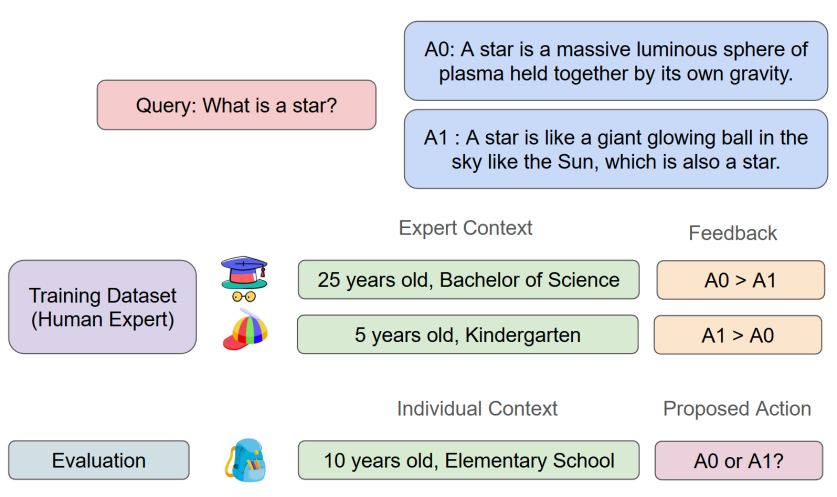
Despite its successes, the existing RLHF framework faces notable challenges (Casper et al., , 2023). As the reward model is a function of the query-answer pair, it assumes that all individuals share a single preference function. In practice, however, individuals exhibit diverse characteristics, leading to heterogenous preferences (Zhong et al., , 2024; Park et al., , 2024). The heterogeneity in human preferences can lead to three types of challenges. The first challenge is the personalization problem. For instance, consider a model tasked with answering the question, “What is a star?”. The model could offer a detailed scientific explanation, such as “A star is a massive, luminous sphere of plasma held together by its own gravity,” or a simpler response like “A star is a giant glowing ball in the sky, like the Sun.” While a scientifically inclined user might favor the former, a five-year-old child is more likely to prefer the latter for its simplicity and interpretability (See Figure 1). This example illustrates the benefits of development of personalized models that adapt to user contexts, highlighting the potential of contextual RLHF to address these diverse needs.
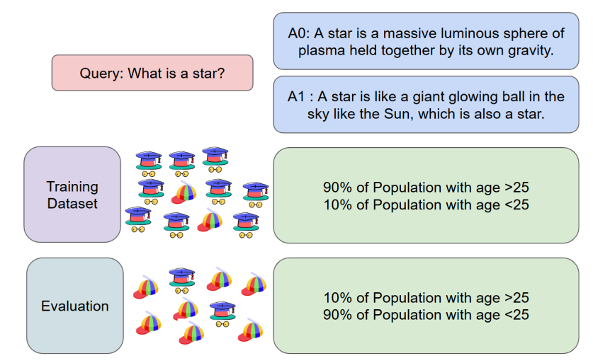
The second challenge is the distribution shift between the offline training data and the target deployment distribution. For example, consider a scenario where offline feedback data are predominantly collected from college students, but the model is intended for deployment among preschool children as illustrated in Figure 2. As the model is trained on the offline dataset via empirical risk minimization, the estimated homogeneous model will lead to optimize its performance on the college students, which could perform poorly with children. In such cases, accounting for user-specific features becomes essential to effectively bridge the gap between the training and target distributions, ensuring the model performs well even on different populations.
The last challenge is the high dimensionality of contexts in RLHF problems. In LLMs, reward models are typically trained using features extracted from the final layer of a pre-trained supervised model. For instance, GPT-3 (175B) (Brown, , 2020) has 12,288 units in its last layer, while InstructGPT, which employs a 6B reward model (RM), has 4,096 units in its last layer (Ouyang et al., , 2022). Additionally, Ouyang et al., (2022) includes contextual information about labelers (human experts), such as demographic attributes (e.g., age, gender, ethnicity, nationality, education level) and survey-based details. Including both user contexts and state-action features in the model leads to a rapidly expanding parameter space, driven by the high-dimensional interaction terms. This growth poses substantial computational challenges for efficient parameter estimation.
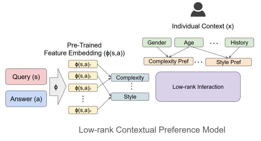
In this paper, we introduce a Low-rank Contextual RLHF (LoCo-RLHF) framework to address these challenges. Advances in digital platforms have enabled the collection of rich and diverse user data, which can be leveraged to develop individualized preference models. Instead of modeling user preferences as a homogeneous function of state-action pairs for state and action , we consider heterogeneous preference , where represents individual context. Specifically, the homogeneous feedback model considers for the pre-trained embedded feature and some unknown vector parameter . To allow heterogeneity induced from individual contexts, we adopt the bilinear form , where and is a unknown matrix parameter. This formulation captures heterogeneity in preference by accounting for individual contexts. To address the high dimensionality, we leverage the low-rank structure of the parameter matrix. Low-rank approximations have been successfully applied in various domains, including contextual bandits (Jun et al., , 2019; Kang et al., , 2022) and LLMs (Li et al., , 2018; Aghajanyan et al., , 2020; Hu et al., , 2021; Ding et al., , 2023; Dettmers et al., , 2024; Sidahmed et al., , 2024). In this approach, high-dimensional features are projected into a low-dimensional latent space. For example, in the context of a query about a star, state-action features might include an embedding representing the complexity of the explanation, while user context features (e.g., age, education level) could capture preferences for simpler or more detailed responses. The interaction between these features and contexts is then modeled using a reduced set of latent factors. Motivated from this, we impose a low-rank structure on the matrix parameter as shown in Figure 3 and hence substantially reduce the computation complexity from to , where is the rank of the matrix. Details of the contextual preference model is given in Section 2.1. By imposing a low-rank structure, we effectively reduce the dimensionality of the parameter space, preserving the essential interactions while minimizing estimation errors and computational costs.
We then design a Pessimism on Reduced Space (PRS) algorithm to solve this LoCo-RLHF problem. The PRS algorithm has the following three key components: estimating the low-rank subspace, constructing confidence bounds and pessimistic values, and deriving the pessimistic policy.
-
1.
Estimating the low-rank subspace. In the first stage, we leverage the low-rank structure of the parameter matrix to estimate a low-dimensional subspace using a rank-constrained maximum likelihood estimator. Since this optimization problem is inherently non-convex, we employ factored gradient descent (also known as alternating gradient descent) via the Burer-Monteiro formulation (Burer and Monteiro, , 2003; Zheng and Lafferty, , 2016). Once the matrix is estimated, we perform singular value decomposition (SVD) to extract orthogonal matrices that define the subspace. These matrices allow us to embed features and contexts into a reduced-dimensional space, thereby reducing the problem’s overall complexity.
-
2.
Constructing confidence bounds. With the reduced subspace established, the next step involves projecting the original problem into the low-dimensional space and constructing confidence bounds within this representation. Subspace estimation inherently introduces uncertainty when projecting to the reduced rank. To address this, we develop a novel analytical framework that incorporates the uncertainty quantification into the confidence bound construction, ensuring robustness in subsequent stages.
-
3.
Deriving the pessmistic policy. Finally, we adopt a pessimistic approach, widely used in offline RL literature (Jin et al., , 2021; Fu et al., , 2022; Zhu et al., , 2023; Shi et al., , 2024), to account for uncertainties in reward estimation. By optimizing the pessimistic reward, constructed to account for worst-case scenarios, we derive a robust policy that balances exploration and exploitation, even in the presence of distribution shift.
In theory, we provide theoretical guarantees for our algorithm by deriving upper bounds on the sub-optimality gap. The sub-optimality gap is defined as the difference between the optimal reward, achieved with complete knowledge of the true parameters, and the reward of the policy derived by our algorithm. Specifically, we establish that the sub-optimality gap of our PRS policy is bounded as with probability at least (Theorem 2). In low-rank settings where , our bound represents a significant improvement over the bound achieved by existing methods (Zhu et al., , 2023). Furthermore, in the special case of our LoCo-RLHF framework where human feedback follows a pre-defined group structure, the derived bound aligns with the results of Zhong et al., (2024), demonstrating the tightness of our analysis.
The sub-optimality gap analysis of our policy presents several challenges. First the rank-constrained maximum likelihood estimation problem is inherently non-convex, which precludes the direct application of classical results from convex optimization literature. Moreover, the offline dataset comprises binary pairwise responses from human experts, rather than direct quantitative data. This characteristic complicates the derivation of the estimation bounds, as it requires handling the discrete nature of the data. During the uncertainty quantification step, both the estimation error of the subspace and the likelihood estimation contribute to the overall uncertainty of the parameter estimate in the reduced space. Lastly, the approximation of the preference function in the reduced space is similarly influenced by the subspace estimation error, which propagates through the analysis and affects the policy’s value. To address these challenges, we develop novel tools that incorporate subspace estimation error into the construction of estimation bounds and the approximation of the preference function.
Finally, we present extensive numerical experiments with varying rank, dimensionality, and offline data distributions to evaluate the proposed PRS policy, comparing it with the greedy policy and the pessimistic policy derived from the unconstrained MLE of Zhu et al., (2023). The results show that the PRS policy consistently outperforms existing methods on the sub-optimality gap, with a larger performance improvement in low-rank, high-dimensional settings, demonstrating the robustness and scalability of our algorithm.
1.1 Related Work
Our work is closely related to, yet distinct from, recent studies on RLHF with heterogeneous experts and low-rank LLMs.
-
•
RLHF with Heterogeneous Experts: The incorporation of human feedback into the RL framework, introduced by Christiano et al., (2017), has gained significant attention in recent years. Recent studies, such as Ouyang et al., (2022) and Bai et al., (2022), highlight that experts may disagree on optimal responses, and biases in offline datasets can disadvantage underrepresented groups (Prabhakaran et al., , 2021; Feffer et al., , 2023; Kirk et al., , 2023). To address the heterogeneity of human preferences, various approaches have been proposed. One common method is to impose a group structure on individuals and train separate reward models for each group, as seen in Park et al., (2024), and Ramesh et al., (2024). These models are then aggregated using techniques such as social welfare functions, Pareto-optimal solutions (Boldi et al., , 2024), or robust optimization (Chakraborty et al., , 2024). Another line of research focuses on personalized models tailored to individual preferences (Jang et al., , 2023; Kirk et al., , 2023; Poddar et al., , 2024). However, most of these approaches lack theoretical guarantees for their performance. The most closely related work is Zhong et al., (2024), which proposes a multi-party RLHF framework that models and aggregates preferences across multiple individuals. While their method addresses heterogeneity through a pre-defined grouping structure, it requires a predetermined clustering of individual preferences and does not fully account for individual-specific contextual information. In contrast, our work extends this research by introducing a low-rank contextual preference model that incorporates expert characteristics and learns the latent low-rank representation of the reward model.
-
•
Low-rank LLMs: To improve LLM performance, many models leverage high-dimensional parameter spaces (Ouyang et al., , 2022; Bai et al., , 2022). As dimensionality increases, low-rank approximations have been proposed for fine-tuning (Hu et al., , 2021; Ding et al., , 2023; Dettmers et al., , 2024), supported by evidence of intrinsic low-dimensional structures within high-dimensional spaces (Aghajanyan et al., , 2020; Sidahmed et al., , 2024). These models primarily focus on low-rank adoption during pre-training or fine-tuning. In contrast, our work addresses the heterogeneity of human feedback in the reward learning step of RLHF. Additionally, drawing from statistical theory on high-dimensional problems (Wainwright, , 2019), we provide a rigorous theoretical analysis. While low-rank structures have been studied in bandit and RL problems (Jun et al., , 2019; Kang et al., , 2022; Cai et al., , 2023; Stojanovic et al., , 2024; Duan et al., , 2024), their application in RLHF remains underexplored.
In summary, our work presents the first provable low-rank contextual RLHF framework that tackles personalization, distribution shift, and high-dimensionality in heterogeneous human preferences.
1.2 Notations
We introduce the notations used throughout the paper. Let denote the set . The Frobenius norm of a matrix is denoted by , and the matrix-induced norm is denoted by . The ball induced by the Frobenius norm, centered at with radius is denoted by . For a vector , represents its -th component. We write if is positive definite. Denote Kronecker product of two matrices as .
2 Problem Formulation
In this section, we formally define the LoCo-RLHF problem within the framework of pairwise comparison feedback. Specifically, we (i) introduce the contextual preference model, which captures the heterogeneous preferences of individuals, and (ii) demonstrate how the contextual reward model addresses both the personalization and distribution shift challenges.
2.1 Contextual Preference Model
To address the heterogeneity in human preferences regarding queries and their corresponding answers, we introduce the contextual preference model. Let denote the state (query) space, the action (answer) space, and the context space. For , a human expert with context is presented with a state and two actions, . The expert selects the preferred action, where indicates a preference for over , and indicates a preference for . The offline dataset comprises a collection of (i) contexts, (ii) states, (iii) action pairs, and (iv) expert preferences, represented as for each individual .
The Bradley-Terry-Luce (BTL) model (Bradley and Terry, , 1952) has been widely used to capture how preferences influence the choices of experts. Let and denote the preferences associated with actions and , respectively. The BTL model assumes that the probability of selecting an action is proportional to the exponential of its preference. Specifically, the probabilities are given by:
The homogeneous preference model (Ouyang et al., , 2022; Achiam et al., , 2023; Touvron et al., , 2023) assumes that the probability of choosing an action depends solely on the query and the available actions, making it identical across individuals. To account for heterogeneity, we introduce a contextual preference model, which reflects individual-specific preferences. Specifically, we model the reward function using a bilinear form:
| (1) |
where represents the individual’s context, is a parameter matrix, and is the feature embedding for the query-action pair. Under this model, the probability of selecting action over , given query and context , is:
This formulation introduces variability in the choice probabilities by incorporating the context , thereby capturing the heterogeneity among individuals.
The high dimensionality of context and feature embeddings poses significant computational challenges, as estimating the matrix parameter scales with the product of their dimensions. Inspired by the successful application of low-rank approximations in reinforcement learning (Jun et al., , 2019; Hu et al., , 2021), we impose a low-rank structure on the parameter matrix. Let be the rank of the parameter matrix , and let represent its singular value decomposition (SVD) of , where and are square matrices, and with as its non-zero diagonal entries. The reward function can then be expressed as:
which simplifies to:
This formulation demonstrates that and project the original features into a low-dimensional subspace, significantly reducing computational complexity, as illustrated in Figure 3.
Remark 1 (Flexibility of the bilinear model).
The bilinear reward model generalizes various existing reward models. First, when with , the model reduces to , corresponding to the reward model for homogeneous individuals (Zhu et al., , 2023). Second, the Boltzmann-model (Jeon et al., , 2020; Barnett et al., , 2023) models the reward as , where is a rationality parameter. If the reward is linear with respect to , such that , and is a linear function of context i.e., , then the reward function becomes: which is the special case of formulation (1) with being a rank-1 matrix. Finally, to model the diversity of human preferences, Zhong et al., (2024) considers types of individuals each with reward given as , where and is a known feature mapping. This setup is also a special case of formulation (1), where , , , and for individual of type , where is the -th standard unit vector in .
2.2 Value of Policy
Next, we show how the contextual preference model effectively tackles personalization and distribution shift challenges. Let be the joint distribution of context and state in the evaluation set. In the personalization problem, the individual feature is available for the policy, enabling the policy to adapt its responses based on the context of each individual. Formally, the policy is defined as , allowing it to provide tailored answers for different contexts. The value of the policy is then defined as:
In the personalization problem, the objective is to determine an individualized policy that provides personalized responses for each individual with context , even when the the same query is presented. The goal is to maximize the value of the policy.
The second case is the distribution shift problem. Unlike the personalization problem, the features of individuals are unavailable during evaluation in this second case. In this case, the policy is defined as a function of alone, i.e., . The corresponding value is given by
In the distribution shift problem, the objective is to find a global policy that provides a unified response for all individuals, maximizing the expected value of the policy. It is important to note that the evaluation distribution may differ from the offline training distribution. If the contextual preference model is not considered, a homogeneous reward model would optimize the policy to maximize value based on the offline data distribution, potentially leading to suboptimal performance in the evaluation environment.
For brevity, we use the notation to represent in the personalization problem and in the distribution shift problem. The sub-optimality of a policy is defined as
where denotes the optimal policy. The objective is to determine a policy that minimizes the sub-optimality by leveraging the offline dataset.
Remark 2 (Connection with Zhong et al., (2024)).
When represents the set of standard unit vectors in and with being the uniform distribution, the formulation aligns with the framework proposed by Zhong et al., (2024) under the Utilitarian welfare objective. However, while their approach assumes that the query and answers are generated from the same distribution for all individuals, our framework accommodates scenarios where different state-action pairs are presented to each human expert. Additionally, our framework can be extended to accommodate alternative objective functions. Specifically, the value function can be generalized as: where is a specified transformation, and represents the minimum value of the reward function. For example, when is the logarithmic function, this formulation corresponds to the Nash welfare objective. The theoretical results remain valid with slight modifications, provided that is a Lipschitz continuous function.
3 Algorithm
In this section, we propose the Pessimism in Reduced Subspace (PRS) policy to address the LoCo-RLHF problem. Before introducing the details, we first outline the three main steps in the PRS algorithm.
-
1.
Estimation of the Low-rank Subspace: We begin by solving the rank-constrained maximum likelihood estimation problem to obtain the low-rank estimate . Using the SVD , we obtain an estimate of the low-rank subspaces, where and represent the linear transformation into the low-rank subspace.
-
2.
Reduction to the Low-rank Subspace: Next, we apply the rotation-truncation-vectorization (RTV) process to the parameter , individual contexts and embedded features with respect to the estimated subspaces and . This transformation reduces dimensionality of the parameter space from to , while introducing minimal error from subspace estimation. Using the reduced space, we compute the MLE of the approximate likelihood function, which is used to efficiently estimate the true preference function.
-
3.
Pessimism in the Reduced Space: Finally we construct the confidence set around the estimate by quantifying the uncertainty in the estimation process. Using this confidence set, we define the pessimistic value function:
which represents the pessimistic estimate of the reward under a given policy. The pessimistic policy is then defined by solving .
3.1 Estimation of the Low-rank Subspace
We begin by splitting the dataset into two partitions: the first observations are used to estimate the low-rank subspace, while the remaining observations are used to estimate the parameter and quantify the uncertainty in the reduced space. Given the dataset , the contextual preference model in the BTL model (1) implies that the negative log-likelihood is given by:
| (2) |
Based on it, the rank-constrained optimization problem can be formulated as
which can be solved using the Burer-Monteiro formulation (Burer and Monteiro, , 2003). This approach factorizes , where and . To ensure identifiability, we introduce a regularization term following Zheng and Lafferty, (2016). The resulting optimization problem is formulated as:
To solve this non-convex optimization problem, we employ the alternating Factored Gradient Descent (FGD) method. FGD performs gradient descent on each component iteratively:
where denotes the learning rate, and are the gradients with respect to and , respectively. By alternately updating each component, the estimated parameter converges to the true parameter, provided that certain conditions on the initial estimate and the learning rate are satisfied (Zheng and Lafferty, , 2016; Zhang et al., , 2023). The full details of the FGD procedure are outlined in Algorithm 1.
return .
In our experiments, we compute the initial estimate using the unconstrained maximum likelihood estimator. Convex optimization algorithms, such as L-BFGS (Liu and Nocedal, , 1989), or gradient-based methods can be applied to obtain this initial parameter estimate.
3.2 Reduction to the Low-rank Subspace
RL algorithms leverage uncertainty quantification to improve performance, such as the “optimism in the face of uncertainty” approach for online RL (Abbasi-Yadkori et al., , 2011) and pessimistic policies for offline RL (Jin et al., , 2021; Rashidinejad et al., , 2021). Existing uncertainty quantification methods are primarily designed for vector parameters, making them less suited to our high-dimensional matrix parameter space . The large number of components in this space as well as the low-rank structure of the matrix parameter create significant challenges for effective uncertainty quantification. To address this, we propose the “rotation-truncation-vectorization” (RTV) method, which projects the parameter onto a low-dimensional subspace, reducing its dimensionality and enabling efficient uncertainty quantification.
To illustrate how the RTV method reduces dimensionality, consider the estimate obtained from Algorithm 1. Let be its SVD. Similarly, let represent the SVD of the true parameter . Intuitively, if and are accurate estimates of and , the rotated matrix is expected to a close approximate of the rank diagonal matrix .
For a detailed explanation, let , , and be partitions of and , where represent the first columns and denotes the remaining columns of the matrix. Let be the rotation of with respect to the estimated subspace given by:
where is the upper-left sub matrix of .
We employ the “subtraction method” commonly used in the low-rank matrix bandit literature (Kveton et al., , 2017; Jun et al., , 2019; Kang et al., , 2022), to reduce the dimension. When are accurate estimates of , the terms and are expected to be negligible, as and are orthonormal matrices. Therefore, the product is also expected to be negligible. Based on this intuition, we introduce the concept of “rotation-truncation-vectorization” (RTV) for matrices. For a given matrix , let be the rotation with respect to orthonormal matrices and . Let , , , be the sub-block matrices of . Finally we define the “rotation-truncation-vectorization” of as
| (3) |
where “” is an abbreviation of “rotation-truncation-vectorization”, indicating that the original matrix has been rotated with respect to and , then truncated and vectorized. Since is expected to be negligible, the estimation of should suffice for approximating , with minimal bias. By reducing the dimension from for to of , algorithms operating in the reduced space gain significant computational advantages.
The contextual preference model can be reformulated as:
Here, is the rotation of with respect to and . Let and denote the rotation-truncation-vectorization of . Then, the contextual reward function can be expressed as:
where the approximation holds as . This reformulation allows us to focus on estimating the low-dimensional parameter , where rather than the full matrix . This significantly reduces the computational complexity while maintaining the model’s accuracy.
After reducing the problem to a low-dimensional subspace, we re-estimate the parameter in this reduced space. For the remaining observations, define and let be the rotation-truncation-vectorization of for . The approximate negative log-likelihood function in the reduced space is defined as:
| (4) |
where . As the approximate likelihood function is convex with respect to , convex optimization methods can be applied to obtain the estimate .
3.3 Pessimism in the Reduced Low-rank Space
Finally, we apply the pessimistic approach, which is widely used in offline reinforcement learning (Li et al., , 2022; Zhu et al., , 2023). Instead of the greedy approach that maximizes the estimated reward function based on the estimated parameter, the pessimistic approach maximizes the pessimistic reward. This reward is defined by penalizing the estimated reward based on the uncertainty quantification of the parameter. Intuitively, actions are penalized if the uncertainty in the estimated reward is high. This approach mitigates the risk of selecting suboptimal actions that may result from inaccurate estimates due to the distribution of the offline dataset.
To quantify uncertainty, we define the empirical second moment in the reduced space: . Using this, we construct the confidence set where represents the Mahalanobis norm weighted by , and is the confidence threshold.
To define the pessimistic reward based on this confidence set, we introduce the approximate reward function with respect to :
where is the rotation-truncation-vectorization of . The pessimistic value function is then defined as:
The complete PRS algorithm is summarized in Algorithm 2.
return The pessimistic policy .
In case where the policy can be parametrized as , finding the pessimistic policy can be solved via gradient based methods.
4 Theory
In this section, we first present the assumptions required to establish the rate of the sub-optimality gap. We then derive the estimation error for the low-rank subspace estimation and provide an upper bound on the sub-optimality gap for the PRS algorithm.
4.1 Assumptions
We begin by introducing the boundedness condition and the positive definite second moment condition of the features and the parameter.
Assumption 1 (Boundedness).
The expert feature is bounded by , i.e., . For any query and answer , the feature embedding is bounded, i.e., . For the matrix parameter , for all .
Assumption 2 (Positive Definite Second Moment).
Suppose the context-state-actions for the data distribution . Let . Then .
The boundedness assumption is common in contextual reinforcement learning problems (Li et al., , 2017; Zhu et al., , 2023; Zhan et al., , 2023; Zhong et al., , 2024). The invertibility of the second moment of the feature is required to guarantee that the parameter is identifiable. Suppose and , with . Then and therefore . In other words, if the features from the state-action pairs and contexts both have positive definite second moment and are independent (Zhu et al., , 2023; Zhong et al., , 2024), Assumption 2 is satisfied. When is uniformly distributed over standard unit vectors of , it becomes equivalent with the problem in Zhong et al., (2024), where they assume each query-answer pair is given to each of the user types.
4.2 Main Results
We first present the estimation bound of the low-rank estimator.
Theorem 1 (Informal Estimation Bound).
Suppose Assumptions 1 and 2 hold. Let denote the rank of , with as its singular values. Assume we have an initial estimate such that for some constant . Then for the low-rank estimator achieved from Algorithm 1 with learning rate , we have the estimation bound:
with probability at least for some constant .
Remark 3 (Initial Estimate ).
We assume the availability of an initial estimate that is reasonably close to . This assumption is standard in low-rank matrix estimation problems (Jain et al., , 2013; Chi et al., , 2019; Xia and Yuan, , 2021) and is commonly referred to as the “basin of attraction” condition, ensuring that the algorithm converges to the desired target. This assumption holds in various scenarios. For instance, when the sample size is sufficiently large, the unconstrained maximum likelihood estimator can serve as a warm start for Algorithm 1, providing an initial estimate close to .
The estimation error bound is proportional to , whereas without the low-rank assumption, it would scale with . This highlights the critical role of the low-rank assumption in reducing estimation error. This rate aligns with bounds in the low-rank matrix estimation literature, particularly under the assumption of bounded -norms for the context and feature embedding . Specifically, if the max-norm of the parameter matrix is bounded, the -norm bound scales with and , consistent with results in Negahban and Wainwright, (2011), Xia and Yuan, (2021), and Zhu et al., (2022). Building on this result, we derive the following corollary concerning the error induced by the rotation-truncation-vectorization process.
Corollary 1 (Error induced by Rotation-Truncation-Vectorization).
Suppose for some . Then,
| (5) |
for some constant .
The details of the proof are provided in Appendices LABEL:sect:EstBound and LABEL:sect:rtv_error. Using these results, we establish the confidence bounds for the estimator in the reduced space.
Lemma 1 (Confidence Bound on ).
Finally, we derive an upper bound on the sub-optimality gap for the proposed policy.
Theorem 2 (Upper Bound of Sub-optimality).
In low-rank case where , our bound represents a significant improvement over achieved by existing methods (Zhu et al., , 2023). Moreover, the setting in Zhong et al., (2024) is a special case of our framework when the true clustering structure of human feedback is known with and . They derived a sub-optimality rate of
where . Assume , and ignoring logarithmic factors, their rate simplifies to . Noting that their value function is defined as the sum over types for the utilitarian welfare function, and we can verify that our rate of matches this bound in this special case.
Remark 4 (Discussion on Concentratability Coefficient).
The concentratability coefficient is invariant under rotation and decreases as covariates are removed. Since the rotation in the bilinear form remains a rotation after vectorization, the rotation-truncation-vectorization (RTV) process reduces the concentratability coefficient. When the matrix is full-rank, RTV simplifies to a pure rotation, ensuring consistency in the concentratability coefficient. Furthermore, this aligns with the concentratability coefficient defined in Zhu et al., (2023) when , i.e., in the absence of contextual information. The theoretical details are provided in Appendix LABEL:sect:ConcenCoeff.
The analysis of our algorithm presents several challenges. First, the rank-constrained maximum likelihood estimation problem is inherently non-convex, which precludes the direct application of classical results from the convex optimization literature. Moreover, the offline dataset comprises binary responses from human experts, rather than quantitative data. This characteristic complicates the derivation of the estimation bounds, as it requires handling the discrete nature of the data. During the uncertainty quantification step, both the estimation error of the subspace and the likelihood estimation contribute to the overall uncertainty of the parameter estimate in the reduced space. Lastly, the approximation of the preference function in the reduced space is similarly influenced by the subspace estimation error, which propagates through the analysis and affects the policy’s value. To address these challenges, we develop novel tools that incorporate subspace estimation error into the construction of estimation bounds and the approximation of the preference function. These tools provide insights into how the subspace estimation error impacts the value of the policy, ensuring a rigorous analysis of our algorithm.
5 Numerical Studies
In this section, we compare the sub-optimality gap of our proposed policy with different benchmarks. We begin by setting , and generating individual contexts and states uniformly from . For actions, we define and specify the feature mapping as:
where is a zero vector, and is the -th standard unit vector (i.e., -th component is and the other components are ). This mapping corresponds to applying one-hot encoding to the categorical variable concatenating with . For the matrix parameter, we use a rank diagonal matrix with all diagonal components set to .
We consider two settings to incorporate different distributions of action pairs in the offline data:
-
•
Uniform Distribution: Action pairs for comparison are generated uniformly from the set . Specifically, two actions are sampled independently without replacement from . This ensures that all actions are well-covered across the offline dataset.
-
•
Imbalanced Distribution: Action pairs are generated with an imbalance parameter . For of the total samples, pairs are uniformly sampled from . For the remaining , the pairs are fixed as . Intuitively, as increases, a majority of the comparisons involve only actions and , while a smaller proportion compares action with other actions, resulting in a highly imbalanced dataset.
We generate parameters, contexts, and features to simulate human feedback and assess the policy on a new set of contexts and states . For comparison, we use two baseline policies.
-
•
MLE-Greedy: This policy uses the MLE obtained from the unconstrained maximum likelihood problem. Since the negative log-likelihood function is convex, the estimator can be efficiently computed. Using the MLE with defined in (2), the policy evaluates the estimated value of each action and selects the greedy action:
-
•
MLE-Pessimistic: Similar to MLE-Greedy, this policy uses the MLE but incorporates the pessimistic approach from Zhu et al., (2023). To adapt the bilinear formulation of the reward to the linear framework used in Zhu et al., (2023), the feature vector is modified to , representing the vectorization of the outer product. This feature vector is used to quantify the confidence bound. Given the pessimistic value function with being the confidence bound on the vectorized feature, this policy maximizes the pessimistic value function:
We evaluate our proposed PRS policy alongside the MLE-Greedy and MLE-Pessimistic policies as baselines. For details of implementing the policy optimization problem , we refer to Appendix LABEL:sect:PolicyOpt. For PRS and MLE-Pessimistic, we use the approximate solution defined in (LABEL:eqn:approximate_policy) of the Appendix. Each simulation is repeated 20 times, and the sub-optimality gap is reported for under various scenarios.
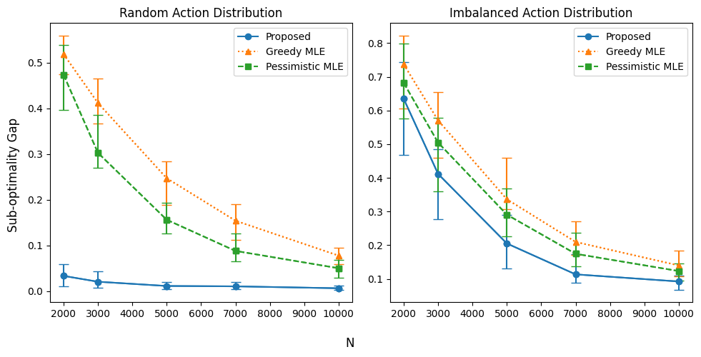
For the first comparison, we fix , and rank , resulting in and . We apply the three methods to both a uniform action distribution and an imbalanced action distribution with . Under the random action distribution, where all parameters associated with each action are well-explored, the sub-optimality gap for MLE-Greedy and MLE-Pessimistic policies shows minimal difference. Interestingly, the greedy policy slightly outperforms the pessimistic policy in this scenario, as there is no benefit of pessimism as the offline dataset sufficiently covers the action space. However, the PRS method, leveraging the low-rank structure for better parameter estimation, significantly outperforms both baseline methods (Figure 4, left). In the imbalanced action setup, the sub-optimality gap increases overall, even with the same sample size, as estimating the parameters becomes more challenging. Here, the pessimistic policy outperforms the greedy policy, reflecting its ability to mitigate the effects of limited exploration. Nevertheless, the PRS policy achieves the best performance, combining the advantages of the low-rank structure with the pessimistic approach (Figure 4, right).
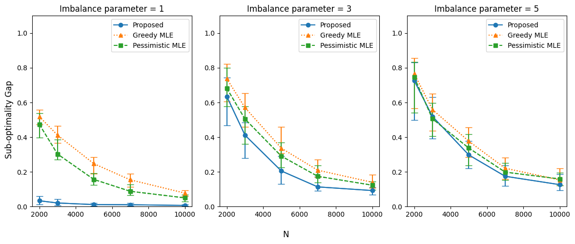
To further examine the effect of offline data imbalance on policy performance, we evaluate the sub-optimality gap of each method under varying imbalance parameters. In this second set of experiments, we use with rank , resulting in . As the dataset becomes more imbalanced, the overall sub-optimality gap increases for all methods. Among the policies, MLE-Greedy consistently performs the worst, while the proposed PRS policy achieves the best performance across all settings. Moreover, the gap between the methods widens as the data imbalance increases, highlighting the robustness of the PRS policy to variations in offline data distribution (Figure 5).
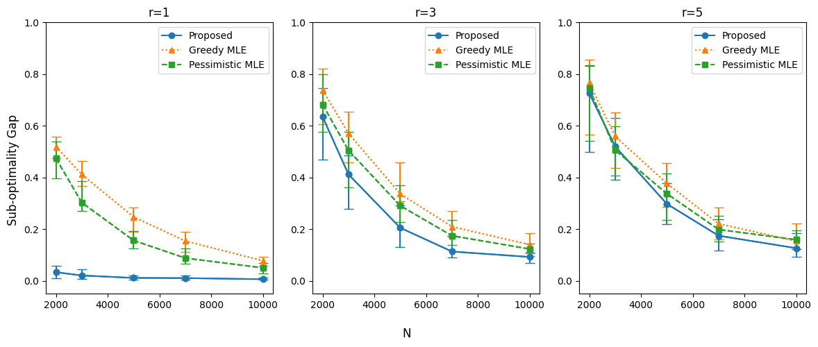
In the final set of experiments, we evaluate the effect of the low-rank assumption on policy performance. Similar to the second set of experiments, we use , but here we fix imbalance parameter and vary the ranks . Across all ranks, the proposed PRS method consistently outperforms the MLE-Greedy and MLE-Pessimistic policies. The sub-optimality gap is nearly zero when , indicating excellent performance under strong low-rank assumptions. However, as the rank increases, the gap between the methods diminishes, reflecting reduced benefits of leveraging the low-rank structure (Figure 6).
6 Conclusion
This paper introduces LoCo-RLHF, a novel framework for addressing heterogeneity in human preferences within reinforcement learning with human feedback (RLHF). The proposed framework enables the design of personalized policies and effectively handles distribution shifts between the training dataset and deployment environments. Through comprehensive theoretical analysis and numerical experiments, we demonstrate that LoCo-RLHF outperforms existing approaches, establishing its robustness in diverse scenarios.
To conclude, we highlight several potential directions for future research. In this work, we evaluate the value of a policy using the expectation of the preference function over a given distribution. This approach can be extended to optimize more complex social welfare functions, such as the Nash welfare function or the Leximin welfare function (Zhong et al., , 2024). Another promising direction is the selection of experts and queries, commonly referred to as active learning (Liu et al., , 2024). Beyond addressing the heterogeneity of contexts, it is crucial to consider non-stationary environments, where the underlying distributions change over time (Bian et al., , 2024). These directions offer exciting opportunities to enhance the robustness and applicability of algorithms in reinforcement learning with human feedback.
References
- Abbasi-Yadkori et al., (2011) Abbasi-Yadkori, Y., Pál, D., and Szepesvári, C. (2011). Improved algorithms for linear stochastic bandits. Advances in neural information processing systems, 24.
- Achiam et al., (2023) Achiam, J., Adler, S., Agarwal, S., Ahmad, L., Akkaya, I., Aleman, F. L., Almeida, D., Altenschmidt, J., Altman, S., Anadkat, S., et al. (2023). Gpt-4 technical report. arXiv preprint arXiv:2303.08774.
- Aghajanyan et al., (2020) Aghajanyan, A., Zettlemoyer, L., and Gupta, S. (2020). Intrinsic dimensionality explains the effectiveness of language model fine-tuning. arXiv preprint arXiv:2012.13255.
- Bai et al., (2022) Bai, Y., Jones, A., Ndousse, K., Askell, A., Chen, A., DasSarma, N., Drain, D., Fort, S., Ganguli, D., Henighan, T., et al. (2022). Training a helpful and harmless assistant with reinforcement learning from human feedback. arXiv preprint arXiv:2204.05862.
- Barnett et al., (2023) Barnett, P., Freedman, R., Svegliato, J., and Russell, S. (2023). Active reward learning from multiple teachers. arXiv preprint arXiv:2303.00894.
- Bian et al., (2024) Bian, Z., Shi, C., Qi, Z., and Wang, L. (2024). Off-policy evaluation in doubly inhomogeneous environments. Journal of the American Statistical Association, pages 1–27.
- Boldi et al., (2024) Boldi, R., Ding, L., Spector, L., and Niekum, S. (2024). Pareto-optimal learning from preferences with hidden context. arXiv preprint arXiv:2406.15599.
- Bradley and Terry, (1952) Bradley, R. A. and Terry, M. E. (1952). Rank analysis of incomplete block designs: I. the method of paired comparisons. Biometrika, 39(3/4):324–345.
- Brown, (2020) Brown, T. B. (2020). Language models are few-shot learners. arXiv preprint arXiv:2005.14165.
- Burer and Monteiro, (2003) Burer, S. and Monteiro, R. D. (2003). A nonlinear programming algorithm for solving semidefinite programs via low-rank factorization. Mathematical Programming, 95(2):329–357.
- Cai et al., (2023) Cai, J., Chen, R., Wainwright, M. J., and Zhao, L. (2023). Doubly high-dimensional contextual bandits: An interpretable model for joint assortment-pricing. arXiv preprint arXiv:2309.08634.
- Casper et al., (2023) Casper, S., Davies, X., Shi, C., Gilbert, T. K., Scheurer, J., Rando, J., Freedman, R., Korbak, T., Lindner, D., Freire, P., et al. (2023). Open problems and fundamental limitations of reinforcement learning from human feedback. arXiv preprint arXiv:2307.15217.
- Chakraborty et al., (2024) Chakraborty, S., Qiu, J., Yuan, H., Koppel, A., Huang, F., Manocha, D., Bedi, A. S., and Wang, M. (2024). Maxmin-rlhf: Towards equitable alignment of large language models with diverse human preferences. arXiv preprint arXiv:2402.08925.
- Chi et al., (2019) Chi, Y., Lu, Y. M., and Chen, Y. (2019). Nonconvex optimization meets low-rank matrix factorization: An overview. IEEE Transactions on Signal Processing, 67(20):5239–5269.
- Christiano et al., (2017) Christiano, P. F., Leike, J., Brown, T., Martic, M., Legg, S., and Amodei, D. (2017). Deep reinforcement learning from human preferences. Advances in neural information processing systems, 30.
- Dettmers et al., (2024) Dettmers, T., Pagnoni, A., Holtzman, A., and Zettlemoyer, L. (2024). Qlora: Efficient finetuning of quantized llms. Advances in Neural Information Processing Systems, 36.
- Ding et al., (2023) Ding, N., Qin, Y., Yang, G., Wei, F., Yang, Z., Su, Y., Hu, S., Chen, Y., Chan, C.-M., Chen, W., et al. (2023). Parameter-efficient fine-tuning of large-scale pre-trained language models. Nature Machine Intelligence, 5(3):220–235.
- Duan et al., (2024) Duan, C., Li, J., and Xia, D. (2024). Online policy learning and inference by matrix completion. arXiv preprint arXiv:2404.17398.
- Feffer et al., (2023) Feffer, M., Heidari, H., and Lipton, Z. C. (2023). Moral machine or tyranny of the majority? In Proceedings of the AAAI Conference on Artificial Intelligence, volume 37, pages 5974–5982.
- Fu et al., (2022) Fu, Z., Qi, Z., Wang, Z., Yang, Z., Xu, Y., and Kosorok, M. R. (2022). Offline reinforcement learning with instrumental variables in confounded markov decision processes. arXiv preprint arXiv:2209.08666.
- Hu et al., (2021) Hu, E. J., Shen, Y., Wallis, P., Allen-Zhu, Z., Li, Y., Wang, S., Wang, L., and Chen, W. (2021). Lora: Low-rank adaptation of large language models. arXiv preprint arXiv:2106.09685.
- Jain et al., (2013) Jain, P., Netrapalli, P., and Sanghavi, S. (2013). Low-rank matrix completion using alternating minimization. In Proceedings of the forty-fifth annual ACM symposium on Theory of Computing, pages 665–674.
- Jang et al., (2023) Jang, J., Kim, S., Lin, B. Y., Wang, Y., Hessel, J., Zettlemoyer, L., Hajishirzi, H., Choi, Y., and Ammanabrolu, P. (2023). Personalized soups: Personalized large language model alignment via post-hoc parameter merging. arXiv preprint arXiv:2310.11564.
- Jeon et al., (2020) Jeon, H. J., Milli, S., and Dragan, A. (2020). Reward-rational (implicit) choice: A unifying formalism for reward learning. Advances in Neural Information Processing Systems, 33:4415–4426.
- Jin et al., (2021) Jin, Y., Yang, Z., and Wang, Z. (2021). Is pessimism provably efficient for offline rl? In International Conference on Machine Learning, pages 5084–5096. PMLR.
- Jun et al., (2019) Jun, K.-S., Willett, R., Wright, S., and Nowak, R. (2019). Bilinear bandits with low-rank structure. In International Conference on Machine Learning, pages 3163–3172. PMLR.
- Kang et al., (2022) Kang, Y., Hsieh, C.-J., and Lee, T. C. M. (2022). Efficient frameworks for generalized low-rank matrix bandit problems. Advances in Neural Information Processing Systems, 35:19971–19983.
- Kiran et al., (2021) Kiran, B. R., Sobh, I., Talpaert, V., Mannion, P., Al Sallab, A. A., Yogamani, S., and Pérez, P. (2021). Deep reinforcement learning for autonomous driving: A survey. IEEE Transactions on Intelligent Transportation Systems, 23(6):4909–4926.
- Kirk et al., (2023) Kirk, H. R., Vidgen, B., Röttger, P., and Hale, S. A. (2023). Personalisation within bounds: A risk taxonomy and policy framework for the alignment of large language models with personalised feedback. arXiv preprint arXiv:2303.05453.
- Kveton et al., (2017) Kveton, B., Szepesvári, C., Rao, A., Wen, Z., Abbasi-Yadkori, Y., and Muthukrishnan, S. (2017). Stochastic low-rank bandits. arXiv preprint arXiv:1712.04644.
- Li et al., (2018) Li, C., Farkhoor, H., Liu, R., and Yosinski, J. (2018). Measuring the intrinsic dimension of objective landscapes. arXiv preprint arXiv:1804.08838.
- Li et al., (2022) Li, G., Ma, C., and Srebro, N. (2022). Pessimism for offline linear contextual bandits using confidence sets. Advances in Neural Information Processing Systems, 35:20974–20987.
- Li et al., (2017) Li, L., Lu, Y., and Zhou, D. (2017). Provably optimal algorithms for generalized linear contextual bandits. In International Conference on Machine Learning, pages 2071–2080. PMLR.
- Liu and Nocedal, (1989) Liu, D. C. and Nocedal, J. (1989). On the limited memory BFGS method for large scale optimization. Mathematical Programming, 45(1):503–528.
- Liu et al., (2024) Liu, P., Shi, C., and Sun, W. W. (2024). Dual active learning for reinforcement learning from human feedback. arXiv preprint arXiv:2410.02504.
- Mnih et al., (2016) Mnih, V., Badia, A. P., Mirza, M., Graves, A., Lillicrap, T., Harley, T., Silver, D., and Kavukcuoglu, K. (2016). Asynchronous methods for deep reinforcement learning. In Balcan, M. F. and Weinberger, K. Q., editors, Proceedings of The 33rd International Conference on Machine Learning, volume 48 of Proceedings of Machine Learning Research, pages 1928–1937, New York, New York, USA. PMLR.
- Mnih et al., (2015) Mnih, V., Kavukcuoglu, K., Silver, D., Rusu, A. A., Veness, J., Bellemare, M. G., Graves, A., Riedmiller, M., Fidjeland, A. K., Ostrovski, G., et al. (2015). Human-level control through deep reinforcement learning. nature, 518(7540):529–533.
- Negahban and Wainwright, (2011) Negahban, S. and Wainwright, M. J. (2011). Estimation of (near) low-rank matrices with noise and high-dimensional scaling. Annals of statistics, 39(2):1069–1097.
- Ouyang et al., (2022) Ouyang, L., Wu, J., Jiang, X., Almeida, D., Wainwright, C. L., Mishkin, P., Zhang, C., Agarwal, S., Slama, K., Ray, A., et al. (2022). Training language models to follow instructions with human feedback, 2022. URL https://arxiv. org/abs/2203.02155, 13:1.
- Park et al., (2024) Park, C., Liu, M., Kong, D., Zhang, K., and Ozdaglar, A. (2024). Rlhf from heterogeneous feedback via personalization and preference aggregation.
- Poddar et al., (2024) Poddar, S., Wan, Y., Ivison, H., Gupta, A., and Jaques, N. (2024). Personalizing reinforcement learning from human feedback with variational preference learning. arXiv preprint arXiv:2408.10075.
- Prabhakaran et al., (2021) Prabhakaran, V., Davani, A. M., and Diaz, M. (2021). On releasing annotator-level labels and information in datasets. arXiv preprint arXiv:2110.05699.
- Ramesh et al., (2024) Ramesh, S. S., Hu, Y., Chaimalas, I., Mehta, V., Sessa, P. G., Ammar, H. B., and Bogunovic, I. (2024). Group robust preference optimization in reward-free rlhf. arXiv preprint arXiv:2405.20304.
- Rashidinejad et al., (2021) Rashidinejad, P., Zhu, B., Ma, C., Jiao, J., and Russell, S. (2021). Bridging offline reinforcement learning and imitation learning: A tale of pessimism. Advances in Neural Information Processing Systems, 34:11702–11716.
- Sallab et al., (2017) Sallab, A. E., Abdou, M., Perot, E., and Yogamani, S. (2017). Deep reinforcement learning framework for autonomous driving. arXiv preprint arXiv:1704.02532.
- Shi et al., (2024) Shi, C., Zhu, J., Shen, Y., Luo, S., Zhu, H., and Song, R. (2024). Off-policy confidence interval estimation with confounded markov decision process. Journal of the American Statistical Association, 119(545):273–284.
- Sidahmed et al., (2024) Sidahmed, H., Phatale, S., Hutcheson, A., Lin, Z., Chen, Z., Yu, Z., Jin, J., Komarytsia, R., Ahlheim, C., Zhu, Y., et al. (2024). Perl: Parameter efficient reinforcement learning from human feedback. arXiv preprint arXiv:2403.10704.
- Silver et al., (2016) Silver, D., Huang, A., Maddison, C. J., Guez, A., Sifre, L., Van Den Driessche, G., Schrittwieser, J., Antonoglou, I., Panneershelvam, V., Lanctot, M., et al. (2016). Mastering the game of go with deep neural networks and tree search. nature, 529(7587):484–489.
- Stojanovic et al., (2024) Stojanovic, S., Jedra, Y., and Proutiere, A. (2024). Model-free low-rank reinforcement learning via leveraged entry-wise matrix estimation. arXiv preprint arXiv:2410.23434.
- Touvron et al., (2023) Touvron, H., Martin, L., Stone, K., Albert, P., Almahairi, A., Babaei, Y., Bashlykov, N., Batra, S., Bhargava, P., Bhosale, S., et al. (2023). Llama 2: Open foundation and fine-tuned chat models. arXiv preprint arXiv:2307.09288.
- Wainwright, (2019) Wainwright, M. J. (2019). High-dimensional statistics: A non-asymptotic viewpoint, volume 48. Cambridge university press.
- Xia and Yuan, (2021) Xia, D. and Yuan, M. (2021). Statistical inferences of linear forms for noisy matrix completion. Journal of the Royal Statistical Society Series B: Statistical Methodology, 83(1):58–77.
- Zhan et al., (2023) Zhan, W., Uehara, M., Kallus, N., Lee, J. D., and Sun, W. (2023). Provable offline reinforcement learning with human feedback. In ICML 2023 Workshop The Many Facets of Preference-Based Learning.
- Zhang et al., (2023) Zhang, J., Sun, W. W., and Li, L. (2023). Generalized connectivity matrix response regression with applications in brain connectivity studies. Journal of Computational and Graphical Statistics, 32(1):252–262.
- Zheng and Lafferty, (2016) Zheng, Q. and Lafferty, J. (2016). Convergence analysis for rectangular matrix completion using burer-monteiro factorization and gradient descent. arXiv preprint arXiv:1605.07051.
- Zhong et al., (2024) Zhong, H., Deng, Z., Su, W. J., Wu, Z. S., and Zhang, L. (2024). Provable multi-party reinforcement learning with diverse human feedback. arXiv preprint arXiv:2403.05006.
- Zhu et al., (2023) Zhu, B., Jordan, M., and Jiao, J. (2023). Principled reinforcement learning with human feedback from pairwise or k-wise comparisons. In International Conference on Machine Learning, pages 43037–43067. PMLR.
- Zhu et al., (2022) Zhu, Z., Li, X., Wang, M., and Zhang, A. (2022). Learning markov models via low-rank optimization. Operations Research, 70(4):2384–2398.
- Ziegler et al., (2019) Ziegler, D. M., Stiennon, N., Wu, J., Brown, T. B., Radford, A., Amodei, D., Christiano, P., and Irving, G. (2019). Fine-tuning language models from human preferences. arXiv preprint arXiv:1909.08593.