Closure of knitted surfaces and surface-links
Abstract.
A knitted surface is a surface with boundary properly embedded in , which is a generalization of a braided surface. A knitted surface is called a 2-dimensional knit if its boundary is the closure of a trivial braid. From a 2-dimensional knit , we obtain a surface-link in by taking the closure of . We show that any surface-link is ambiently isotopic to the closure of some 2-dimensional knit. Further, we consider another type of the closure of a knitted surface, called the plat closure. It is known that any trivial surface-knot is ambiently isotopic to the plat closure of a knitted surface of degree 2. We show that the plat closure of any knitted surface of degree 2 is a trivial surface-link, and any trivial surface-link is ambiently isotopic to the plat closure of a knitted surface of degree . We also show the same result for the closure of 2-dimensional knits of degree 2.
Key words and phrases:
surfaces in 4-space; surface-links; surface braids; tangles; knits; closure; plat closure2020 Mathematics Subject Classification:
Primary: 57K45, Secondary: 57Q35 57K101. Introduction
Let be a positive integer. An -knit [1, 13] is a tangle obtained from an -braid in a cylinder by splicing at some crossings. Splicing a crossing results in a “hook pair”, and we describe the information of each hook pair by a segment called a pairing [14]. We give an equivalence relation to the set of -knits so that two -knits are equivalent if they are related by an isotopy of -knits. The set of equivalence classes of -knits forms a monoid by the multiplication induced from the composition of knits, which is called the -knit monoid. The -knit monoid is generated by elements, , , , where and are the standard generator and its inverse of the -braid group , and is the hook pair between the th and th strings as in Figure 1 . Let be the unit element of , which is represented by the trivial braid. The -knit monoid has the monoid presentation

A knitted surface [14] in a bidisk is defined as an analogue to the notion of an -knit in . A knitted surface is an extended notion of a braided surface [15], which is a surface in in the form of a branched covering over . A knitted surface is constructed as the trace of deformations of knits, as follows. Let be a sequence of elements of the free monoid consisting of and such that and are related by one of the following for each :
-
(1)
One of the relations of the -knit monoid .
-
(2)
Replacement of and , or replacement of and , for some and .
-
(3)
Replacement of and for some .
We decompose into subintervals: , . A knitted surface in is constructed for each as follows. We denote by the same notation a geometric -knit given by the presentation . For case (1), let be an isotopy of -knits in relating and which describes the knit monoid relation. Then we construct by . This construction is called the trace of . The construction is determined by giving , which is called a slice of at .
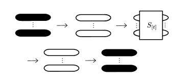
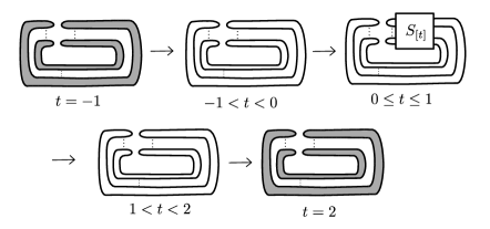
For case (2), we construct by giving slices as follows: , and is the union of and a twisted band (respectively, an untwisted band) corresponding to the (respectively ). See Figure 2. The -knit is the result of band surgery along a band attaching to , and the band corresponds to a branch point of the knitted surface.
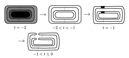
For case (3), let , and let be the union of and a disk whose boundary is the simple closed curve formed by the . See Figure 3.
The knitted surface is the trace of deformations of knits where a simple closed curve is born or dies.
A surface-link is a closed surface smoothly embedded in . In particular, a surface-link with one component is called a surface-knot. A braided/knitted surface is called a 2-dimensional braid/knit if its boundary is the closure of the trivial braid. From a 2-dimensional braid , we obtain an orientable surface-link in by taking the closure of , and Kamada [7] showed that every orientable surface-link is ambiently isotopic to the closure of some 2-dimensional braid. For a 2-dimensional knit , we can also define the closure of by a similar way, which provides a surface-link. In this paper, we show Claim 9.1 in [14] as follows.
Theorem 1.1.
Every surface-link in is ambiently isotopic to the closure of some 2-dimensional knit.
Further, we consider another type of the closure of a knitted surface, called the plat closure. In [14, Theorem 8.1], we showed that any trivial surface-knot is ambiently isotopic to the plat closure of some knitted surface of degree 2. In this paper, we show the following.
Theorem 1.2.
The plat closure of any knitted surface of degree 2 is a trivial surface-link, and any trivial surface-link is ambiently isotopic to the plat closure of a knitted surface of degree 2.
Theorem 1.2 follows from Corollary 5.7 and Theorem 5.13, where Theorem 5.13 is [14, Claim 8.3]. We show this by using a chart description of a knitted surface, which is a generalization of a chart description of a simple braided surface [6, 9]. As a corollary of Theorem 1.2, we have the following.
Corollary 1.3.
The closure of any 2-dimensional knit degree 2 is a trivial surface-link, and any trivial surface-link is ambiently isotopic to the closure of some 2-dimensional knit of degree 2.
The paper is organized as follows. In Section 2, we review knitted surfaces. In Section 3, we review the closure of knitted surfaces, and we show Theorem 1.1. In Section 4, we review a chart description of knitted surfaces of degree 2. In Section 5, we show Theorems 5.13 and 1.2 and Corollary 1.3. We give references [3, 5, 10] for the basics of 1-dimensional and 2-dimensional knot theory. In this paper, we assume that surfaces and tangles are smooth.
2. Knitted surfaces
In this section, we review knitted surfaces [14].
2.1. Motion picture method
In order to describe surfaces in 4-space, we use motion pictures, regarding surfaces as the trace of slices of the surfaces by 3-spaces along the 4th dimensional axis. In this section, we review motion picture method.
Let be a surface properly embedded in , and we denote , where . We modify the saddle points and minimal/maximal points of into saddle bands and minimal/maximal disks, repsectively; see [5, Section 8.4]. Let be the projection. For each , the slice of at , denoted by , is defined as the image by of the intersection : that is, that is, .
When each slice is either (1) a tangle (or a link) or (2) a union of a tangle and several disks (and bands), we describe by a finite sequence of diagrams of consisting unions of (2) and tangles before and after the time of (2). This sequence of diagrams is called a motion picture of .
2.2. Band surgery of a tangle along a band set
Let be a tangle in . A band attaching to is a 2-disk in such that consists of a pair of intervals in . The result of band surgery along , denoted by , is the tangle . We remark that by a slight modification we assume that is also smoothly embedded.
Let be a set of mutually disjoint bands attaching to . Put . The result of band surgery along bands of is given by
2.3. Knitted surface presented by a transformation of knits
For an -knit , we regard as a geometric knit and we identify with its presentation where for each . We call , (), and () a word of , a letter of , and a subword of , respectively. For subwords and of two -knits and , respectively, we call a sequence a transformation if is obtained from by changing to . In this situation, we call a sequence a transformation of an -knit. For subwords of and transformations , …, , we say that the transformations are mutually disjoint if and do not overlap each other for , that is, when and , the intersection of intervals is the empty set.
When we have a transformation of -knits as follow, we construct a knitted surface of degree in in such a way as follows; since the construction is unique up to equivalence, we call the knitted surface presented by . In the following (Case 2) and (Case 3), denotes the sequences and .
(Case 1) A transformation , where and is related by an isotopy of -knits : and .
In this case, we define by
for any .
(Case 2) A transformation or . This is a transformation such that is obtained from by band surgery along a band as in Figure 2.

In this case, we define by the motion picture as given in Figure 2; we define by slices as follow: for , we denote by a band attaching to so that the result of the band surgery along is . Then we define by
and for , the presented surface is given by the mirror image of with respect to , that is, the surface given by the slice for each .
(Case 3) A transformation . In this case, we define by the motion picture as given in Figure 3; we define by slices as follow: we define for ; the other case is given by the same method as in (Case 2). We denote by a disk whose boundary is the simple closed curve in . Further, we assume that . Then we define by

For a transformation such that is obtained from by a finite number of mutually disjoint transformations as given in (Case 1)–(Case 3), the knitted surface presented by is defined as the surface determined from those of (Case 1)–(Case 3). We remark that the construction is called the “vertical product” [5, Section 15.1].
2.4. Knitted surfaces
Knitted surfaces are defined by using “pairings” and “knit structure” [14]. Two knitted surfaces are said to be equivalent if they are related by an “isotopy of knitted surfaces”. Every knitted surface is equivalent to a knitted surface in a normal form. In this paper, we give a knitted surface as a knitted surface derived from a normal form, by using deformations of knits.
Definition 2.1.
Let be a surface properly embedded in . Then, is called a knitted surface of degree if there exists a partition for some satisfying the following conditions, where .
-
(1)
Each slice is an -knit .
-
(2)
The surface is the knitted surface presented by for such that the knit is obtained from by a finite number of mutually disjoint transformations associated with the relations of the -knit monoid as follows , where denotes the sequences and :
-
•
,
-
•
,
-
•
-
•
-
•
,
-
•
-
•
,
-
•
,
-
•
-
•
,
where , .
-
•
We denote by the starting point set of -knits, that is a fixed set of interior points of such that for any -knit . We call the knitted surface the trivial knitted surface.
A knitted surface of degree is called a braided surface of degree if the transformations are restricted to the relations of the -braid group ; that is, the relations do not contain .
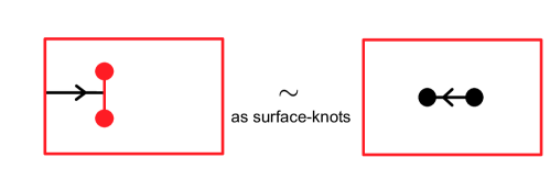
A knitted surface of degree is called a 2-dimensional knit if . A 2-dimensional knit is called a 2-dimensional braid if it is a braided surface.
3. The closure of 2-dimensional knits
In this section, we show Theorem 1.1.
3.1. Closure of knits and 2-dimensional knits
Let . Let be copies of -disks . Let be an -knit in or a 2-dimensional knit in , and let be the trivial knits/2-dimensional knits. Then, is a closed 1-manifold or a closed surface in , where .
Let be a circle (respectively a 2-sphere) standardly embedded in when (respectively ), and let be a regular neighborhood of . We identify with . The closure of is a link or a surface-link in which is given by .
As an analogue of Alexander’s theorem for oriented links, it is known that:
Theorem 3.1 ([8]).
Every orientable surface-link is ambiently isotopic to the closure of some 2-dimensional braid.
3.2. The plat closure of braids
For a set , we denote by the union . A wicket is a semi-circle properly embedded in which meets orthogonally. A configuration of wickets is a set of mutually disjoint wickets. denotes the space consisting of configurations of wickets. Let be a set of interior points of such that lie in in this order. Let denotes the configuration of wickets such that and and are boundaries of the same component of for each . We denote by the mirror image of with respect to ; remark that and are disjoint. The union represents the -knit .
For a -braid , the plat closure of , denoted by , is a link in obtained by taking the union of , , and . See Figure 4. The plat closure can be regarded as the closure of the knit , that is, .

3.3. The plat closure of braided surfaces
We recall the definition of the plat closure of a braided surface [16]. To take the plat closure, a braided surface is required to be “adequate”.
For a loop , we define the -braid by . A braid is called adequate if there exists a loop such that . The set of adequate -braids forms a group called the Hilden subgroup of the -braid group , denoted by , and is generated by , , and for and [2] (see Figure 5 for the case ).

Let be an adequate -braid in . There exists a unique loop satisfying . Let with . Let , an annulus. We define the surface in by
| (3.1) |
A braided surface is called adequate if is the closure of an adequate braid. We remark that an adequate braided surface is of degree for some , and every 2-dimensional braid of degree is adequate.
For an adequate braided surface in , we denote by the adequate braid whose closure is . We take the surface given by (3.1). Recall that . We identify with , and we identify with , and we embed by and . We remark that . Then the plat closure of is a surface-link in defined by the union of and , denoted by .
Theorem 3.2 ([16]).
Every surface-link is ambiently isotopic to the plat closure of some adequate braided surface.
3.4. Proof of Theorem 1.1
Let be a surface-link. By Theorem 3.2, we take an adequate braided surface of degree such that the plat closure is ambiently isotopic to .
(Case 1) First, we consider the case that is a 2-dimensional braid, that is, has the motion picture as in Figure 6. Put .
We take a surface-link given by
where is a union of copies of disks whose boundaries are ; see Figure 7. The surface is ambiently isotopic to the plat closure .
Let be the surface properly embedded in given by
where is a union of disks whose boundaries are and is a band set attaching to such that , and is the union of bands of ; see Figure 8. The surface consists of copies of disks. We denote by the surface . Then both and consist of copies of disks with . These set of disks are called trivial disk systems, and it is known [11] that they are ambiently isotopic rel .
Similarly, we take the surface properly embedded in given by the mirror image of with respect to , and we denote by the surface . Then and are ambiently isotopic rel . Let be a surface obtained from by replacing and with and , respectively; that is,
By construction, is ambiently isotopic to .
Let be the cylinder associated with the knits in slices. Put . Then is a 2-dimensional knit given by
Further, we see that the closure of is . Thus, the closure of the 2-dimensional knit is ambiently isotopic to the given surface-link .
(Case 2) Next, we consider the case when is ambiently isotopic to the plat closure of an adequate braided surface of degree . By considering a self-homeomorphism of and the induced self-homeomorphism of given by , we assume that has a presentation of an adequate braid whose closure is . We denote the adequate braid by . By the same isotopy used to obtain from in (Case 1), we have a surface-link . Let be a knitted surface in associated with the adequate braid given in [14, Section 6.4.2]. Then, the surface satisfies
Thus, let be the knitted surface given by
The Let be the surface given by
where is a union of copies of disks whose boundaries are .
By construction of , is a trivial disk system (see [14, Proposition 6.6]) and is ambiently isotopic to the surface-link .
Then, by the same process with Case 1, we obtain a new surface-link from by replacing and with and , respectively. The surface-link is ambiently isotopic to . Then, is a 2-dimensional knit and the closure of is the surface-link . Hence, the closure of the 2-dimensional knit is ambiently isotopic to the given surface-link . ∎
4. Chart description
A knitted surface of degree is presented by a finite graph on called a “chart” of degree [14], which is a generalization of a chart for braided surfaces [6, 7, 9]. Here, we give the definition of charts of degree 2. See [14] for the definition of degree .
Definition 4.1.
Let be a finite graph in a 2-disk . Then, is a knit chart of degree , or simply a 2-chart, if it satisfies the following conditions.
-
(1)
The intersection consists of a finite number of endpoints of edges of meeting orthogonally. Though they are vertices of degree one, we call elements of boundary points, and we call only a vertex in a vertex of .
-
(2)
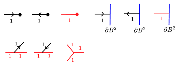
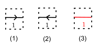
Each edge is equipped with the label and moreover, each edge is either oriented or unoriented. We call an oriented/unoriented edge a -/-edge, respectively.
-
(3)
Each vertex is of degree 1 or 3 as depicted in Figure 9.
A vertex of degree 1 connected with a -edge (respectively -edge) is depicted by a small black (respectively red) disk, called a black -vertex (respectively black -vertex). A vertex of degree is called a mixed trivalent vertex (respectively a trivalent -vertex) if it is connected with a -edge and a pair of -edges (respectively three -edges).
A knitted surface has a chart description. From a knitted surface of degree , we obtain a chart of degree , and from a given chart , we can construct a knitted surface whose chart is ([14]).
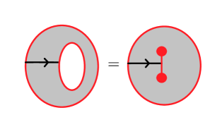
In the rest of this paper, we focus on knitted surfaces of degree and their -charts. Thus we only review the knitted surface of degree 2 constructed from a -chart as follows. We decompose into a union of a finite number of 2-disks such that for each disk , by modification, is either an empty graph (called an empty chart) or one of the -charts as in Figures 9 and 10, where the dotted square in Figure 10 denotes . We identify with , where the direction of is the vertical direction from up to down and the direction of is the horizontal direction from left to right in the figures. When is an empty chart, we define by the trivial knitted surface . When is one of the -charts as in Figure 10, we define by the knitted surface for Figure 10(1), for Figure 10(2), and for Figure 10(3). When is one of the -charts as in Figure 9, we define by the knitted surface presented by for the -chart containing one black /-vertex for appropriate , and the knitted surface presented by , , or for the -chart containing a trivalent vertex. We construct the knitted surface presented by as the union of the knitted surfaces presented by .
4.1. Chart moves
In this section, we give the definition of chart moves for -charts, that are local moves of charts. This includes C-moves of charts of braided surfaces [5, 6, 9].
Definition 4.2.
Let and be -charts in . Then, a knit chart move, or a C-move, is a local move in a 2-disk such that (respectively ) is changed to (respectively ), satisfying the following.
-
(1)
The boundary does not contain any vertices of and except for boundary points, and (respectively ) consists of transverse intersection points of edges of (respectively ) and .
-
(2)
The charts are identical in the complement of : .
- (3)
We say that and are C-move equivalent if they are related by a finite sequence of C-moves and ambient isotopies of .
Let and be -charts and let and be the knitted surfaces presented by and , respectively. Theorem 7.5 in [14] implies that and are ambiently isotopic if and are -move equivalent. Thus, the plat closures of and are ambiently isotopic if and are -move equivalent.
5. Plat closure of knitted surfaces of degree
In this section, we consider knitted surfaces of degree .
We give a normal form of a -chart (Definition 5.1 and Proposition 5.2).
We show that any trivial surface-link is ambiently isotopic to the plat closure of knitted surfaces of degree 2 (Corollary 5.7).
We show that the plat closure of any knitted surface of degree 2 is a trivial surface-link (Theorem 5.13), and we show Theorem 1.2 and Corollary 1.3.
5.1. Knitted surfaces of degree
A -/-edge of a chart is called a free -/-edge if its endpoints are black -/-vertices. A -edge of a chart is called a half -edge if its endpoints consists of a black -vertex and either a boundary point or a mixed trivalent vertex. A -edge of a chart is called a half -edge if its endpoints consists of a black -vertex and either a boundary point or a trivalent –vertex.
For a chart , the -chart of , denoted by , is defined as the subgraph of consisting of -edges and the connecting vertices. The -chart may contain -valent vertices which are obtained from mixed trivalent vertices. Then, we merge the two edges connected by each 2-valent vertex after removing the -valent vertex. Thus, consists of intervals, circles, and graphs consisting of -valent vertices and -valent vertices. We call a connected component of a -component. When is contained in , a region of is the closure of a connected component of .
Definition 5.1.
Let be a -chart, let be regions of the -chart , and put , the subchart of . Then, we say that is in a normal form if for each , there exists a -component of such that every -edge of is either a free -edge or connected with , and half -edges connected with have coherent orientations. We call the initial -component of .
See Figure 12 for an example.
Proposition 5.2.
Any 2-chart is C-move equivalent to a -chart in a normal form given in Definition 5.1.
Proof.
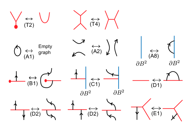
Let be a -chart. The labels of edges are all one. We denote by the same notation the charts obtained from by C-moves. From now on, we consider each subchart of as given in Definition 5.1. We fix a -component of . By the definition of -charts, -edges are classified by combinations of their endpoints; a -edge is either a simple closed curve (called a circle component), a free -edge, a half -edge, a -edge connecting with /-components. Let be a -edge of disjoint with . Since is connected, we take a simple path from a point of to . Applying (A1), (A2) and (D1)-moves, each circle component of -edges is deformed into a -edge connecting -components. By applying (A2) and (D1)-moves, we deform half -edges and -edges connecting -components into -edges connected with , see Figure 13; the detail is left to the reader as exercise. Further, by (A2)-moves, we deform half -edges connected with to a set of free -edges and half -edges with coherent orientations. Thus we arrange into a normal form. ∎
Remark 5.3.
We can deform a 2-chart to a more regulated form, also denoted by , satisfying that (1) every black -vertex is an endpoint of a free -edge, (2) free -/-edges are in a -disk which contains no other parts of , (3) -edges connecting a -component and the initial -component have coherent orientations, and (4) there are no -edges both of whose endpoints are connected with the initial -component.
5.2. The plat closure of knitted surfaces
Let be a knitted surface of degree . We define the plat closure of in such a way as follows. If is a braided surface, then is adequate; thus we define the plat closure of by that of a braided surface, given by , where is the surface of (3.1) in Section 3.3. Further, if is the closure of a -braid, then we define the plat closure of by the same way, given by . We consider the case that is the closure of a -knit having hook pairs. Then, consists of m simple closed curves, where m is the number of hook pairs in . We define the plat closure of by the closed surface obtained from by attaching copies of -disks trivially along .
For knitted surfaces of degree , we do not give the exact definition in terms of wickets in this paper, but we briefly give the idea of the plat closure, as follows. We call an -knit adequate if it is an element of the submonoid of the -knit monoid generated by adequate -braids and . We call a knitted surface adequate if is the closure of an adequate knit. For an adequate knitted surface , we construct the plat closure of as follows. Let be the adequate knit whose closure is . We denote by the braid obtained from the adequate knit by changing each letter in the form of for some to . We denote by the letters of coming from the letters of in the form of . The -braid is adequate. Let be the surface associated with given in (3.1) in Section 3.3. The part of corresponding to , that is for some with , is a band with one twist. We delete the band from and take the closure for each . Then, slightly modifying , we obtain a surface in with . We define the plat closure of by the surface-link in .
Remark 5.4.
The plat closure of a knitted surface of degree is a special case of the closure of a -dimensional knit of degree by the following meaning. Let be a -chart of , a point disjoint with , and let be a small neighborhood of disjoint from . Let be a -disk such that is contained in the interior of . Let be the -chart in obtained from by adding to a union of -edges in the form . Since does not have boundary points, it represents a -dimensional knit of degree , denoted by . By applying the argument in the proof of Theorem 1.1, the plat closure of S and the closure of is ambiently isotopic as surface-links. In particular, when has no boundary points, then is obtained from by an addition of a single free -edge.
We can calculate the Euler characteristics of knitted surfaces of degree by using the information derived from charts. The proof is left to the reader; see [5, Exercise 9.15]. For simplicity, we consider a knitted surface , presented by a -chart in a 2-sphere .
Proposition 5.5.
Let be a knitted surface of degree , and let be its -chart. Let be regions of the -chart , and put , the subchart of . Then is a split union of , where is the plat closure of a knitted surface , , and the Euler characteristic is calculated by
where is the number of black -vertices of , and is the Euler characteristic of the closure of , where is a regular neighborhood of .
5.3. Plat closure of knitted surfaces of degree presenting trivial surface-links
A standard 2-sphere (respectively a standard torus) in is the boundary of a 3-ball (respectively an unknotted solid torus) in , and a standard positive projective plane (respectively a standard negative projective plane) is the surface given by Figure 14(1) (respectively (2)). These surfaces are called standard surfaces. A surface-knot in is called trivial if it is a connected sum of a finite number of standard surfaces in , and a surface-link is trivial if it is a split union of a finite number of trivial surface-knots.

When a half -edge has an orientation toward (respectively from) the black -vertex, we call it positive (respectively negative). We denote by a standard torus, and by (respectively ) a standard positive (respectively negative) projective plane.
Theorem 5.6 ([14]).
Let be a trivial surface-knot, which is a connected sum of copies of and copies of and copies of . Then is the plat closure of the knitted surface presented by a -chart such that consists of copies of free -edges, copies of free -edges, and copies of positive (respectively negative) half -edges if (respectively ).
Corollary 5.7.
Any trivial surface-link is ambiently isotopic to the plat closure of some knitted surface of degree .
Proof.
Let be a trivial surface-link, and let denote connected components of . Let be the segment in . Then, divide into -disks , . Applying Theorem 5.6, we obtain a -chart in such that the plat closure of a knitted surface is ambiently isotopic to . Let be the union of and -edges in the form of . Then, the plat closure of is a split union of the plat closures of , , which is ambiently isotopic to . ∎
5.4. Knit plat index and the knit index
The plat index [16] of a surface-link , denoted by , is the half of the minimum of the degrees of braided surfaces whose plat closures are ambiently isotopic to . We define the knit plat index, denoted by , as the half of the minimum of the degrees of knitted surfaces whose plat closure is ambiently isotopic to . By definition, for a surface-link ,
It is known [16] that the plat index of surface-link is one if and only if it is a trivial 2-sphere or nonorientable trivial surface-knot, and the plat index is two if the surface-link is a trivial orientable surface-knot with positive genus. Corollary 5.7 implies the following:
Corollary 5.8.
Let be any trivial surface-link. Then, the knit plat index of is one:
The braid index [5] of an oriented surface-link , denoted by , is the minimum of the degrees of 2-dimensional braids whose closures are ambiently isotopic to . We define the knit index of a surface-link , denoted by , by the minimum of the degrees of 2-dimensional knits whose closures are ambiently isotopic to . By definition, for an oriented surface-link ,
By the argument in the proof of Theorem 1.1, we have the following.
Corollary 5.9.
Let be any surface-link. Then, the knit index of is bounded from above by twice the plat index of :
By Corollary 1.3, we have the following.
Corollary 5.10.
Let be a trivial surface-link. Then, if is not a trivial 2-sphere, then,
5.5. Remark on 2-charts presenting trivial surface-knots
The trivial surface-knot is presented by a 2-chart other than that given in Theorem 5.6.
Proposition 5.11.
The trivial surface-knot is ambiently isotopic to the plat closure of the knitted surfaces of degree presented by the 2-charts as in Figure 15.
Proof.
The trivial surface-knot has the motion picture as in Figure 16(1). The surface is ambiently isotopic to the surface as in Figure 16(2). This surface is ambiently isotopic to the surface as in Figure 16(3), which is the surface given by the gray regions of the 2-charts in Figure 17; so it is the plat closure of the knitted surface presented by the -chart in the left figure of Figure 15. By Theorem 5.6, is ambiently isotopic to the plat closure of the knitted surface presented by the -chart in the right figure of Figure 15. Thus the -charts as in Figure 15 both present . ∎

Let be a trivial surface-knot, which is a connected sum of copies of and copies of and copies of . If , then is a connected sum of copies of and copies of (respectively ) if (respectively ). We can show this by using -charts, applying Theorem 5.6, Proposition 5.11 and C-moves. The proof is left to the reader as exercise. In the following, we give the result in terms of -charts.
Corollary 5.12.
Let be a -chart consisting of copies of free -edges, copies of free -edges and copies of positive (respectively negative) half -edges. If , then the plat closure of the knitted surface presented by is ambiently isotopic to the plat closure of the knitted surface presented by the -chart consisting of copies of free -edges and copies of positive (respectively negative) half -edges.
5.6. Proof of Theorem 1.2 and Corollary 1.3
Let be a surface-link in . A 1-handle attaching to is a 3-ball embedded in such that . The arc is called the core of the 1-handle. The 1-handle surgery is the operation which changes to a new surface-link given by . A 1-handle attaching to is called trivial if we can move the 1-handle by ambient isotopy so that is contained in a 4-ball in such that the pair is homeomorphic to the standard -ball pair .
Theorem 5.13.
Let be the plat closure of an arbitrary knitted surface of degree 2. Then, is a trivial surface-link.
Proof.
Let be an arbitrary -chart. It suffices to show the result for the subchart of each region divided by the -chart of . So we assume that is in a normal form such that is connected. We call a -edge which is not a half -edge a non-half -edge. Let be segments in such that each coincides with each non-half -edge. Since we take the plat closure, we regard as the initial -component.
Let be the 2-chart obtained from by changing each non-half -edge into a -edge. Let (respectively ) be the plat closure of the knitted surface presented by (respectively ). We see that is a split union of the plat closures of knitted surfaces of -charts of regions divided by the -chart of , and is obtained from by 1-handle surgery along 1-handles such that the projection to of the core of transversely intersects with the segment . We remark that since is in a normal form, each region is a 2-disk. We consider the case , when the number of non-half -edges is one. We put , the 1-handle along which is obtained from by 1-handle surgery. The plat closure is a surface-knot, and is either a surface-knot or a surface-link with two components. By Theorem 5.6, using (T2)-moves (see Figure 11) if necessary, we see that and are trivial surface-knots/links. If is a surface-link with two components, denoted by and , then, is a connected sum of and . If is a surface-knot, then, since is trivial, the 1-handle is trivial [4]. Hence, the result of 1-handle surgery, , is a connected sum of and either a standard torus or a connected sum (see Figures 16(3) and 17). For the general case, since is a trivial surface-link by Theorem 5.6, by induction on the number of non-half -edges, we see that is obtained from components of by taking connected sum with several copies of and . Hence we see that is a trivial surface-knot. Thus we have the required result. ∎
Proof of Corollary 1.3.
By Remark 5.4, Corollary 5.7 implies that any trivial surface-link is ambiently isotopic to the closure of some 2-dimensional knit. Let be a 2-chart in . Theorem 1.1 implies that if contains at least one -edge, then the closure of the 2-dimensional knit presented by is a trivial surface-link. If does not contain -edges, then it presents a 2-dimensional braid, the closure of which is an orientable trivial surface-link [5]. ∎
Acknowledgements
The first author was partially supported by JST FOREST Program, Grant Number JPMJFR202U. The second author was partially supported by JSPS KAKENHI Grant Number 22J20494.
References
- [1] J. S. Birman, H. Wenzl, Braids, link polynomial and a new algebra, Trans. Amer. Math. Soc. 313 (1989) 249–273.
- [2] T. Brendle, A. Hatcher, Configuration spaces of rings and wickets, Comment. Math. Helv., 88 (2008) 131-162.
- [3] J. S. Carter, S. Kamada, M. Saito, Surfaces in 4-space, Encyclopaedia of Mathematical Sciences 142, Low-Dimensional Topology III, Berlin, Springer-Verlag, 2004.
- [4] S. Kamada, Cords and 1-handles attached to surface-knots, Bol. Soc. Mat. Mex. 20 (2014) 595-609.
- [5] S. Kamada, Braid and Knot Theory in Dimension Four, Math. Surveys and Monographs 95, Amer. Math. Soc., 2002.
- [6] S. Kamada, An observation of surface braids via chart description, J. Knot Theory Ramifications 5 (1996), no. 4, 517–529.
- [7] S. Kamada, A characterization of groups of closed orientable surfaces in 4-space, Topology 33 (1994) 113–122.
- [8] S. Kamada, Alexander’s and Markov’s theorems in dimension four, Bull. Amer. Math. Soc. (N.S.), 31 (1994), no. 1, 64–67.
- [9] S. Kamada, Surfaces in of braid index three are ribbon, J. Knot Theory Ramifications 1 (1992), no. 2, 137–160.
- [10] A. Kawauchi, A Survey of Knot Theory, Birkhäuser Verlag, Basel, 1996.
- [11] A. Kawauchi, T. Shibuya, S. Suzuki, Descriptions on surfaces in four-space. I. Normal forms, Math. Sem. Notes Kobe Univ., 10 (1982), no. 1, 75–125.
- [12] H. M. Hilden, Generators for two groups related to the braid group, Pacific J. Math., 59 (1975), no. 2, 475–486.
- [13] J. Murakami, The Kauffman polynomial of links and representation theory, Osaka J. Math. 24 (1987) 745–758.
- [14] I. Nakamura and J. Yasuda, Surfaces in the 4-ball constructed using generators of knits and their graphical description, arXiv: 2306.10479v2.
- [15] L. Rudolph, Braided surfaces and Seifert ribbons for closed braids, Comment. Math. Helv. 58 (1983) 1–37.
- [16] J. Yasuda, A plat form presentation for surface-links, arXiv:2105.08634, to appear in Osaka J. Math.