Introduction to Graph Neural Networks: A Starting Point for Machine Learning Engineers

Abstract

Graph neural networks are deep neural networks designed for graphs with attributes attached to nodes or edges. The number of research papers in the literature concerning these models is growing rapidly due to their impressive performance on a broad range of tasks. This survey introduces graph neural networks through the encoder-decoder framework and provides examples of decoders for a range of graph analytic tasks. It uses theory and numerous experiments on homogeneous graphs to illustrate the behavior of graph neural networks for different training sizes and degrees of graph complexity.

Keywords— Graph neural networks, graph representation learning, deep learning, encoders, graphs

1 Introduction

Relationships within data are important for everyday tasks like internet search and road map navigation as well as for scientific research in fields like bioinformatics. Such relationships can be described using graphs with real vectors as attributes associated with the graph’s nodes or edges; however, traditional machine learning models operate on arrays, so they cannot directly exploit the relationships. This report surveys Graph Neural Networks (GNNs), which jointly learn from both edge and node feature information, and often produce more accurate models. These architectures have become popular due to their impressive performance on graph analysis tasks. Consequently, the number of research papers on GNNs is growing rapidly, and many surveys exist.

Some surveys discuss graph neural networks in the context of broad families such as graph networks, graph representation learning and geometric deep learning [1, 2, 3, 4, 5]. Other surveys categorize GNNs by abstracting their distinguishing properties into functional relationships [6, 7, 8, 3, 9]. Although useful for organizational purposes, generality and abstraction can be difficult to understand for those new to the field. Other surveys have a narrow focus, for example to discuss efforts to improve a specific weakness in GNN architectures [10], or to survey GNN work on a particular task, such as fake news detection or product recommendation [11, 12]. While valuable for those interested in the task, they provide little background in GNNs and therefore assume the reader already has that knowledge.

For this reason, a concrete and concise introduction to GNNs is missing. We begin by introducing GNNs as encoder-decoder architectures. To provide perspective on the ways GNNs are used, we discuss common GNN applications along with examples of task-specific decoders for turning features into predictions. We think that studying a few important examples of GNNs well will help the reader develop a feeling for the subject that would be difficult to achieve otherwise. We therefore focus on three convolutional and attentional networks, GCN, GraphSAGE, and GATv2, which are commonly used both as benchmarks and as components in other GNN architectures. We conduct numerous experiments with these GNNs at two training sizes and on thirteen datasets of both high and low complexity. The experiments have three goals:

• Compare benchmark GNNs with other graph models.

• Demonstrate how hyperparameter adjustments affect GNN performance.

• Provide a qualitative picture of what happens when GNNs learn.

We hope these experiments combined with the theoretical sections will enable newcomers to use GNNs more effectively and to improve GNN performance on their problems. We also hope that experts will gain new insights from our experiments.

2 Common applications

Graph neural networks are suited to a variety of graph tasks.

1. Node classification

   This task concerns categorizing nodes of a graph. There are several applications within the space of social networks, such as assigning roles or interests to individuals or predicting whether individuals are members of a group [13, 14]. Node classification tasks also include classifying documents, videos or webpages into different categories [15, 16]. There are also important applications in bioinformatics, such as classifying the biological function of proteins (nodes) and their interactions (edges) with other proteins [17].

2. Link prediction

   Link prediction is a classification task on pairs on nodes in a graph. Most often, this is a binary classification problem, where the task is to predict whether an edge exists between two nodes, e.g. one to predict that an edge is present and zero to predict that it is absent. Link prediction also exists for graphs with multiple edge types, so edges are predicted to be one of several types [18].

   Link prediction can predict the presence of a relationship (edge) between two individuals (nodes) in a social network, either presently or in the near future [19]. Recommendation systems try to recommend products to customers; this task is a link prediction problem, where one seeks edges between two different types of nodes, the product nodes and the customer nodes [20, 21]. Link prediction for entity resolution predicts links between different records in a dataset that refer to the same object [22, 23]. For example, we want to link a record describing ”John Smith” with another record for the same person written ”Smith, John”. In bioinformatics, link prediction can predict relationships between drugs and diseases [24] and the similarity between diseases [25]. Link prediction also includes finding new relationships between nodes in knowledge graphs, a task called knowledge graph completion [26, 27].

3. Community detection

   Community detection algorithms cluster graph nodes by using some problem dependent similarity measure. They are typically not machine learning based [28, 29], but some algorithms may be trained in an unsupervised or semi-supervised manner [30, 31]. Applications include identifying social groups within a social network [32], entity resolution [33], fraud detection [34], text clustering (e.g. grouping Reddit posts into similar topics) [17] and visualization [35, 36].

4. Node regression and edge regression

   The traffic prediction literature tries to predict traffic conditions, like traffic speed, volume, etc., in the near future from sensors on the road, which supports tasks such as travel time estimation and route recommendations [37, 38]. The road network has intersections as nodes and road segments as edges. The sensors are additional nodes on the road network, so estimating the numeric descriptors of traffic conditions at these sensors is a node regression problem. Less often, edge regression models support traffic prediction by predicting edge weights that represent traffic flow or count, [39]. Other node regression applications include predicting house prices and weather characteristics [40], and predicting the amount of internet traffic to web pages [41].

5. Graph classification and graph regression

   Conventionally, time consuming and expensive laboratory experiments establish a molecule’s properties. Molecule property prediction is foundational for the development of new materials with industrial applications and new drugs to treat diseases, and consequently, significant resources have been devoted to developing a model that can accurately predict molecule properties quickly and cheaply. Graphs naturally represent molecules with its nodes as atoms and its edges as chemical bonds between two atoms, and GNNs, which operate directly on graphs, quickly proved to be well suited to this task [42, 43, 44, 45]. The accuracy of GNN predictions matches or exceeds that of conventional models with expert features when enough labeled data is available for training [43], but labeled data is often limited in the target domain, so prediction accuracy suffers [46]. To meet this challenge, self-supervised approaches that leverage large amounts of unlabeled data are being developed [46, 47, 48].

3 Introduction to encoder-decoder models

An attributed graph has a set of nodes, $\mathcal{N}$, as well as edges that define how the nodes relate to each other. To simplify the discussion, we restrict our attention to undirected graphs, so the edges are represented by a weighted, symmetric adjacency matrix, $A=(A_{ij})$ where $i,j\in\mathcal{N}$. An entry $A_{ij}$ is non-zero if an edge connects node $i$ to node $j$ and zero otherwise. Each node, $i\in\mathcal{N}$ has an attribute, $x_{i}\in{\mathbb{R}}^{\ell}$ for some $\ell\in{\mathbb{N}}$. Encoder-decoder models on graphs is a class of machine learning models. Machine learning on graphs presents challenges that do not arise in conventional machine learning on vectors, because graphs are irregular data structures and do not have a natural coordinate system. In particular, standard convolutional neural networks for image arrays do not work on graphs, because the $k$-hop neighborhoods may be different for every node. Nonetheless, a typical first step for machine learning on graphs is to obtain a low-dimensional feature vector for every node that contains all the information that is needed to complete the desired task. These feature vectors are real vectors that often contain the information needed to represent the local edge structure about each node.

A feature vector of a node is also called a node embedding or a node representation, and collectively the feature vectors can be used for tasks on nodes, tasks on edges, or tasks on the entire graph. At the graph level, applying principal component analysis (PCA) or t-distributed stochastic neighbor embedding (t-SNE) to node embeddings can produce lower dimensional representations that enable visualizations to help understand the how algorithms are performing [49]. In addition, community detection algorithms use node embeddings to define the communities, either in an end-to-end fashion [50] or as part of a two-step process by applying the $k$-means algorithm to the node embeddings [51, 52]. Node embeddings also support graph classification, where in the simplest case, a mean activation over all node embeddings of the graph determines the graph class. More sophisticated approaches are described in [53, 54]. Not surprisingly, node features are also used for node level tasks like node classification and regression, [55, 15], as well as for edge level tasks like link prediction [56], edge classification [57, 58] or edge regression [59].

Due to the importance of node embeddings, there are many techniques to obtain them for a range of goals and data conditions. Perhaps the simplest example of a node embedding is given by the rows of an adjacency matrix. The map $:i\to(A_{ij})_{j\in\mathcal{N}}$ defines node embeddings in ${\mathbb{R}}^{|\mathcal{N}|}$. However, it is difficult to use these vector representations in machine learning due to their sparsity or high dimension, which tends to lead to overfitting. The row vectors are also poor features, because they do not provide any structural information beyond each node’s 1-hop neighborhood nor do they account for any node attributes.

Instead, researchers may use rule-based descriptions of nodes, like centrality or clustering measurements, to produce low dimensional node representations that are more information dense, which may subsequently be applied to a downstream task with a traditional machine learning algorithm. The disadvantage of this approach is that hand-crafted features are not part of the algorithm’s training process, so the features are not fine-tuned to minimize the loss function. To do this, researchers use an encoder-decoder approach.

3.1 Encoder-decoder framework

Figure 1:

Many machine learning models adhere to an encoder-decoder framework shown in Figure 1. The encoder is a function

$$\operatorname{Enc}:\mathcal{N}\to{\mathbb{R}}^{\ell}$$ (1)

that maps nodes to node embeddings in ${\mathbb{R}}^{\ell}$, where $\ell\ll|\mathcal{N}|$. A good encoder creates node embeddings that contain all of the information about each node that is required to complete the task at hand.

Subsequently the decoder function

$$\operatorname{Dec}:{\mathbb{R}}^{m}\to{\mathbb{R}}^{k}\,,$$ (2)

converts those node embeddings into predictions, where $m\geq\ell$ and $k$ is the dimension of the model predictions. We emphasize that the decoder generally does not simply invert the encoder. It is instead a kind of interpreter that “decodes” abstract node embeddings into predictions in order to solve the given task. The decoders for common tasks like those described in Section 2 are usually simple functions with few parameters, such as an inner product followed by a softmax function. Hence, the majority of the model’s learnable parameters are usually in the encoder.

We introduce the term ground truth function

$$\operatorname{Gt}:\mathcal{G}\to{\mathbb{R}}^{k}\,,$$ (3)

that provides reference information that is known about the graph, such as a node’s class for node classification, which the loss function compares with the $k$-dimensional model predictions. The training and evaluation algorithms use it to assess the quality of model predictions. There does not seem to be an accepted term in the literature that accounts for all contexts that occur. Hamilton, et al. [55] consider the case of a relationship between two nodes and call it a pairwise similarity function. This occurs in link prediction, where the ground truth function may be a map $:\mathcal{N}\times\mathcal{N}\to\{0,1\}$ that says whether or not an edge exists between two nodes. In node classification, however, the ground truth function typically provides the node’s class. In all cases, its role in the encoder-decoder framework is the same, so we refer to it by a single name.

The loss functions and evaluation metrics link the ground truth function and the model prediction. Most algorithms learn model parameters by some form of gradient decent, where the loss functions are fairly smooth. Common examples of loss functions are cross entropy loss for classification and $L^{1}$ or $L^{2}$ loss for regression tasks. For evaluation metrics, common examples are accuracy, F1 and AUC (Area Under the receiver operator characteristic Curve) for classification and RMSE (Root Mean Square Error) and MAE (Mean Absolute Error) for regression tasks.

3.2 Shallow embedding examples

We now present several representative examples of models that produce embedding lookups for nodes that were seen during the training process. These examples will illustrate the encoder-decoder framework and at the end we will note their shortcomings, which Hamilton et al. [55, 2] describes. This will lead us to more complicated encoder-decoder models called GNNs in the next section.

For each example, the input is a fixed matrix that provides a similarity statistic between any two nodes in $\mathcal{N}$ such as a weighted adjacency matrix. The output of these algorithms is a real vector (a feature vector) for each node describing the node’s neighborhood structure, and taken together, they support some downstream machine learning task.

The Laplacian eigenmaps algorithm is an early and successful nonlinear dimensionality reduction algorithm [60]. Given a user-defined parameter $t>0$, a weighted adjacency matrix, $W=(W_{ij})_{i,j\in\mathcal{N}}$, can be defined by

$$W_{ij}=W_{ij}(t)=\left\{\begin{aligned} &\exp\left(-\frac{\|x_{i}-x_{j}\|^{2}}{t}\right)&\textrm{ if }A_{ij}=1\,,\\ &0&\textrm{ otherwise}\,.\end{aligned}\right.$$ (4)

In practice, the above weighted adjacency matrix is typically the input to the Laplacian eigenmaps algorithm, but a simple adjacency matrix or a $k$-nearest neighbor matrix may alternatively be inputs.

The Laplacian eigenmaps algorithm can be reformulated in terms of the encoder- decoder framework [55, 2]. Define the ground truth, decoder and loss functions by

$$\operatorname{Gt} :\mathcal{N}\times\mathcal{N}\to{\mathbb{R}}, \quad\operatorname{Gt}(i,j)=W_{ij}\,,$$ (5)

$$\operatorname{Dec} :{\mathbb{R}}^{\ell}\times{\mathbb{R}}^{\ell}\to{\mathbb{R}}^{+}, \quad\operatorname{Dec}(w,z)=\|w-z\|^{2}\,,$$ (6)

$$L :{\mathbb{R}}\times{\mathbb{R}}^{+}\to{\mathbb{R}}, \quad L(q,r)=qr\,.$$ (7)

Then the goal is to to find the (non-constant) encoder $\operatorname{Enc}$

$$z_{i}=\operatorname{Enc}(i)\in{\mathbb{R}}^{\ell}\,,\quad\quad\textrm{ for }i\in\mathcal{N}$$ (8)

that minimizes the model’s loss $\mathcal{L}\in{\mathbb{R}}^{+}$ up to a scaling factor, where that loss is

$$\mathcal{L} =\sum_{i,j\in\mathcal{N}}L\big{(}\operatorname{Gt}(i,j),\operatorname{Dec}(z_{i},z_{j})\big{)}$$ (9)

$$=\sum_{i,j\in\mathcal{N}}W_{ij}\|z_{i}-z_{j}\|^{2}\,,$$

where the minimization is subject to a constraint that prevents the solution from collapsing to a lower dimension (i.e. $Z^{T}DZ=I$, where $Z=(z_{i})_{i\in\mathcal{N}}$). Notice that $W_{i,j}\geq 0$ is larger when $i$ and $j$ are adjacent. Then the above equation means that the model is punished during training for having node attributes of adjacent nodes be far apart. (Note that the constant encoder $\operatorname{Enc}(i)=\mathbf{1}$ satisfies $\mathcal{L}=0$, but this is not useful).

Belkin et al. [60] provides an optimal solution based on generalized eigenvectors of the graph Laplacian. The graph Laplacian is the matrix $\Delta=D-W$, where $D$ is a diagonal matrix defined by $D_{ii}=\sum_{j}W_{ji}$ [61]. The generalized eigenvectors $(f_{k})_{1\leq k\leq|\mathcal{N}|}\subset{\mathbb{R}}^{|\mathcal{N}|}$ are the solutions to the equation

$$\Delta f=\lambda Df\,,$$ (10)

where they are labeled in sorted order so that the corresponding eigenvalues satisfy

$$0=\lambda_{0}\leq\lambda_{1}\leq\cdots\leq\lambda_{|\mathcal{N}|-1}\,.$$ (11)

The encoder $\operatorname{Enc}:\mathcal{N}\to{\mathbb{R}}^{\ell}$ uses the first $\ell$ generalized eigenvectors:

$$\operatorname{Enc}(i)=\big{(}f_{1}(i),\ldots,f_{\ell}(i)\big{)}\,.$$ (12)

Inspired by the success of Laplacian eigenmaps, several papers define node similarity using inner products in a class of techniques called matrix factorization methods [62, 63, 64]. Matrix factorization approaches typically rely entirely on the graph’s edge structure. The three cited methods differ only in how they define the ground truth function, $\operatorname{Gt}$. Hamilton et al. [55] reformulates each approach into a encoder-decoder framework:

$$\operatorname{Gt} :\mathcal{N}\times\mathcal{N}\to{\mathbb{R}}^{+}, \quad\operatorname{Gt}(i,j)\in{\mathbb{R}}^{+},$$ (13)

$$\operatorname{Dec} :{\mathbb{R}}^{\ell}\times{\mathbb{R}}^{\ell}\to{\mathbb{R}}, \quad\operatorname{Dec}(w,z)=w^{T}z,$$ (14)

$$L :{\mathbb{R}}^{+}\times{\mathbb{R}}\to{\mathbb{R}}^{+}, \quad L(q,r)=\frac{1}{2}(q-r)^{2}.$$ (15)

Given an encoder $\operatorname{Enc}$ with node embeddings

$$z_{i}=\operatorname{Enc}(i)\in{\mathbb{R}}^{\ell}\,,\quad\quad\textrm{ for }i\in\mathcal{N}\,,$$ (16)

the loss $\mathcal{L}\in{\mathbb{R}}^{+}$ is

$$\mathcal{L} =\sum_{i,j\in\mathcal{N}}L\big{(}\operatorname{Gt}(i,j),\operatorname{Dec}(z_{i},z_{j})\big{)}$$ (17)

$$=\frac{1}{2}\sum_{i,j\in\mathcal{N}}\big{(}z_{i}^{T}z_{j}-\operatorname{Gt}(i,j)\big{)}^{2}\,.$$

Notice that if $Z=(z_{i})$ is the matrix of features in ${\mathbb{R}}^{\ell\times|\mathcal{N}|}$, then the above loss satisfies

$$\mathcal{L}=\frac{1}{2}\|Z^{T}Z-S\|^{2}\,,$$ (18)

where $S$ is the matrix with entries $S_{ij}=\operatorname{Gt}(i,j)$. Minimizing $\mathcal{L}$ means finding a matrix $Z$ that factors the ground truth of matrix $S$ as shown in Equation (18), which is why the methods are called matrix factorization methods.

Ahmed et al. [62] define the ground truth function by $\operatorname{Gt}(i,j)=A_{i,j}$, where $(A_{ij})_{i,j\in\mathcal{N}}$ are the coefficients of the adjacency matrix. Hence, their goal is to find a solution that minimizes the loss

$$\mathcal{L}=\frac{1}{2}\sum_{i,j\in\mathcal{N}}\left(z_{i}^{T}z_{i}-A_{i,j}\right)^{2}\,.$$ (19)

More recently in 2014, Perozzi et al. [16] introduce random walks on a graph as a tool to learn node embeddings that capture the edge structure of larger node neighborhoods in a computationally efficient manner. After a random initialization of node features, a stochastic gradient descent algorithm updates features to optimize the information necessary to estimate the probability that two nodes co-occur on the same random walk of a fixed length. Two years later Grover et al. [65] improved on Perozzi et al. by adding explore and return parameters that respectively determined the algorithm’s tendency to explore new nodes and return to the starting node. Later, [66] showed that these random walk methods are essentially matrix factorization techniques.

Matrix factorization methods have the advantage of being applicable on graphs without attributes. On attributed graphs, however, all of the examples of shallow models share several shortcomings [55]:

1. They make insubstantial use of the node attributes during training, so they do not use all available information. Moreover, these models tend to define similarity in terms of proximity, and consequently they usually produce poor results when adjacent nodes in a graph tend to be dissimilar [67].

2. Trained models cannot be applied to unseen nodes without further training. This is impractical for dynamic graphs and for graphs that are so large that they cannot fit in memory. It also means that a model trained in a setting with a lot of labeled data is not transferrable to an unseen graph in a related domain with sparsely labeled data.

3. The information is not efficiently stored in the model. Each trained model is the collection of node features for the graph, which means model parameters are not shared across nodes. In particular, the number of parameters grows linearly with $|\mathcal{N}|$, which can create memory challenges for processing on large graphs.

The next section discusses more powerful encoder-decoder approaches called graph neural networks, which resolve these shortcomings.

4 Graph Neural Networks

Graph neural networks have several desirable properties. They jointly use node attributes and edge information for training, trained models can be applied to unseen graphs, and the number of parameters of a GNN is independent and sub-linear in the number of nodes. Moreover, they apply naturally to both undirected and directed graphs.

This section focuses on GNNs that have so-called message-passing layers (described below). The vast majority of GNNs in the literature have message-passing layers.

4.1 Encoder layers

A typical GNN encoder can have three classes of layers: pre-processing layers, message-passing layers and post-processing layers. The pre- and post-processing layers are optional.

Figure 2: Three classes of layers in a GNN encoder.

In general, a single layer feedforward neural network has the form

$$:{\mathbb{R}}^{d}\to{\mathbb{R}}^{\tilde{d}},\quad x_{i}:\to\sigma(Wx_{i}+b)\,,$$ (20)

where for positive integers $d$ and $\tilde{d}$, $W:{\mathbb{R}}^{d}\to{\mathbb{R}}^{\tilde{d}}$ is a matrix and $b\in{\mathbb{R}}^{\tilde{d}}$ is a vector, both with of trainable parameters, and $\sigma$ is an element-wise non-linear function (e.g. element-wise ReLU). Pre-processing layers are a stack of one or more of these networks

$$\operatorname{Pre-Proc}:{\mathbb{R}}^{m}\to{\mathbb{R}}^{\widetilde{m}},\quad\operatorname{Pre-Proc}(x_{i})=\tilde{x}_{i}\,,$$ (21)

that maps each node attribute vector $x_{i}$ to a node feature vector $\tilde{x}_{i}$ in a computation that does not involve the edges of the graph.

These node features feed into the message-passing layers, which are the most important layers for the GNNs performance [68]. If $A$ is a graph with a matrix of node features $\widetilde{X}=(\tilde{x}_{i})_{i\in\mathcal{N}}$, then a message-passing layer is a map

$$\operatorname{Message-Passing}:(\widetilde{X},A)\to(H,A)$$ (22)

from the graph $A$ with node features $\widetilde{X}$ to the graph $A$ with node features $H=(h_{i})_{i\in\mathcal{N}}$, where the node feature vectors $h_{i}\in{\mathbb{R}}^{\widetilde{\ell}}$ are obtained by aggregating information from each node’s neighborhood. Then node features from each successive message-passing layer contain information that has been aggregated over a wider set of nodes than the previous layers. At the end, an encoder of a $k$-layer GNN that aggregates node features over a 1-hop neighborhood produces low dimensional node embeddings that summarize information in each node’s $k$-hop neighborhood. In this way, message-passing layers resemble the highly successful convolutional neural networks for image classification.

Node features from the message-passing layers subsequently feed into the final layers of the GNN encoder called the post-processing layers. They are collectively, like the pre-processing layers, fully connected feedforward neural networks

$$\operatorname{Post-Proc}:{\mathbb{R}}^{\widetilde{\ell}}\to{\mathbb{R}}^{\ell},\quad\operatorname{Post-Proc}(h_{i})=z_{i}$$ (23)

that maps each node feature vector $h_{i}$ that is produced by the message-passing layers to the node embedding $z_{i}$. Then the encoder of the GNN maps each node with its node attribute $x_{i}$ to a node embedding $z_{i}$

$$\operatorname{Enc}:\mathcal{N}\to{\mathbb{R}}^{\ell},\quad\operatorname{Enc}(i)=z_{i}.$$ (24)

Each message-passing layer of the encoder computes its output using the same process. Consider a $K$-layer message-passing network. For each node $i$, define $h^{(0)}_{i}=\tilde{x}_{i}$, and for integers $0<k<K$, let $h^{(k)}_{i}\in{\mathbb{R}}^{\tilde{\ell}_{k}}$ be the node feature vector that is the output of the $k_{th}$ message-passing layer. Starting from the output of the $k_{th}$ message-passing layer, for each node $i$, the $k+1$ message-passing layer computes the vectors $h^{(k+1)}_{i}$ by

$$h_{i}^{(k+1)}=\phi\left(\bigwedge\left(h_{i}^{(k)},\bigoplus_{j\in\mathrm{N}_{i}}\mu_{ij}\right)\right)\,.$$ (25)

Sometimes called the update function, $\phi:{\mathbb{R}}^{\tilde{\ell}_{k}}\to{\mathbb{R}}^{\tilde{\ell}_{k+1}}$ is a differentiable function with trainable parameters. A common choice for $\phi$ is a single layer, feedforward neural network, as in (20). The term $\bigoplus$ is a permutation-invariant aggregation function such as an element-wise vector-valued sum, mean or maximum, $\mathrm{N}_{i}$ is the 1-hop neighborhood of $i$ (excluding $i$), and the term $\mu_{ij}\in{\mathbb{R}}^{\tilde{\ell}_{k}}$ is a feature vector (defined below) that describes the interaction of node $i$ with node $j$. The function $\bigwedge$ is determines how each node interacts with the aggregation of its neighbors, for example by concatenation or by element-wise summation. Equation (25) is more concisely written without the function $\bigwedge$, but unlike other authors [4], we include it because our experiments show the choice of $\bigwedge$ is at least as important to the behavior of the GNN as the node-to-node interaction terms, $\mu_{ij}$.

There are three common architecture categories for GNNs in the literature: Convolutional, Message-Passing (MP), and Attentional, and the majority of GNNs fit into one of them. The way that the features at nodes $i$ and $j$ interact (i.e. $\mu_{ij}$) defines a GNN’s type. We denote the message-passing category by its initials, MP, to help distinguish it from message-passing layers. Our description of each GNN category follows Bronstein et al. [4]. This discussion is intended to capture key ideas rather than all subtle similarities and differences between individual models.

An architecture is in the convolutional category,

$$h_{i}^{(k+1)}=\phi\left(\bigwedge\left(h_{i}^{(k)},\bigoplus_{j\in\mathrm{N}_{i}}w_{ij}\psi(h_{j}^{(k)})\right)\right),$$ (26)

if the value $\mu_{ij}$ from (25) is defined by $\mu_{ij}=w_{ij}\psi(h_{j}^{(k)})$, where $\psi$ is a differentiable function that can have trainable parameters, such as an affine linear transformation, $\psi:{\mathbb{R}}^{\tilde{\ell}_{k}}\to{\mathbb{R}}^{\tilde{\ell}_{k}}$,

$$\psi(h_{j}^{(k)})=Wh_{j}^{(k)}+b\,,$$ (27)

where $W:{\mathbb{R}}^{\ell_{k}}\to{\mathbb{R}}^{\ell_{k}}$ is a matrix and $b\in{\mathbb{R}}^{\ell_{k}}$ is a vector. The coefficients $w_{ij}$ are unlearned weights, usually depending only on the local graph topology and which encode the connection strength between pairs of nodes [69, 15, 17, 68, 70]. If the graph exhibits homophily, meaning that nodes with similar features or the same class label tend to be linked [71], then in principal, the fixed weights $w_{ij}$ make these models a good choice due to their scalability and regularization. This occurs, for example, in a social network with users connected by friendship [72]. On the downside, the rigidness of fixed weights may inhibit their ability to represent the complex relationships that arise in low homophily graphs.

An architecture in the MP category computes vectors by

$$h_{i}^{(k+1)}=\phi\left(\bigwedge\left(h_{i}^{(k)},\bigoplus_{j\in\mathrm{N}_{i}}\psi(h_{i}^{(k)},h_{j}^{(k)})\right)\right),$$ (28)

where $\psi:{\mathbb{R}}^{2\tilde{\ell}_{k}}\to{\mathbb{R}}^{\tilde{\ell}_{k}}$ is a differentiable function with trainable parameters such as an affine linear transformation. These are the most expressive of the three flavors of GNNs, which makes them suitable for complex modeling tasks like predicting the properties of molecules or complex dynamical systems [73, 74]. However, this flexibility also makes them more challenging to train, and they require relatively large amounts of memory, which makes them difficult to run at scale compared to those in the convolutional category.

Finally, a model in the attentional category balances the expressiveness of a MP architecture with the scalability of a convolutional one. The features are computed by

$$h_{i}^{(k+1)}=\phi\left(\bigwedge\left(h_{i}^{(k)},\bigoplus_{j\in\mathrm{N}_{i}}a(h_{i}^{(k)},h_{j}^{(k)})\psi(h_{j}^{(k)})\right)\right),$$ (29)

where the algorithm learns the scalar-valued function $a$ and the possibly the function $\psi$ [75, 76, 77, 78, 79]. For example [78], the function $a$ may be computed by

$$a(h_{i}^{(k)},h_{j}^{(k)})=\frac{\exp(\alpha_{ij})}{\sum_{m\in N_{i}}\exp(\alpha_{im})}\,,\quad\textrm{where }\alpha_{im}=\sigma(\mathbf{a}^{T}\cdot W(h_{i}^{(k)}||h_{m}^{(k)}))\,.$$ (30)

Here, $\sigma$ is a nonlinear function, $||$ is concatenation, and for $d$ hidden dimensions, $\mathbf{a}$ is a $d\times 1$ dimensional vector and $W$ is a $d\times 2\tilde{\ell}_{k}$ dimensional matrix. Because $a$ is scalar-valued, learning interactions involves fewer parameters than for the MP networks. This makes attentional networks easier to train and run than the MP networks at the cost of being less expressive. On the other hand, attentional networks may be a little more difficult to run at scale than convolutional ones, but because attentional networks learn edge weights, they tend to outperform convolutional ones on low homophily graphs [79, 80].

While the interaction between each node and the aggregation of its neighbors (i.e. $\bigwedge$) does not define the GNN category, it can significantly affect GNN behavior. For example, the attentional networks GAT and GATv2 get flexibility from the attention mechanism of their node-to-node interactions, $\mu_{ij}$, but they use vector addition for $\bigwedge$. In contrast, GraphSAGE is convolutional but uses concatenation for $\bigwedge$, so (25) becomes

$$\sigma\left(W(h_{i}^{(k)}||\bigoplus_{j\in\mathrm{N}_{i}}\mu_{ij})+b\right)\,.$$ (31)

This enables GraphSAGE to better preserve the information of each node when mixing it with that of its neighbors hurts performance. Section 5.2 presents results from numerous experiments that show GraphSAGE tends to outperform the attentional networks GAT and GATv2 on low homophily graphs, see also [17, 77, 78].

Table 1: $\bigwedge$ Versus GNN Category for Some Common GNNs

$\bigwedge$ Convolutional Attentional Sum GCN GAT, GATv2 Concatenation GraphSAGE

Lastly, we remark that a version of convolutional GNNs also exist for the spectral domain, where an aggregation function operates on the eigenvectors of the graph Laplacian [81]. Comparing with the convolutional GNNs described above, the spectral version may provide richer features, but it also is more memory intensive and does not readily extend to directed graphs nor allow predictions on unseen nodes [82, 83].

4.2 Decoder and loss functions

Below are minimalist examples of these components for several graph tasks from Section 2. More sophisticated examples appear in the literature. For an integer $K>0$, the softmax function, $\operatorname{softmax}:{\mathbb{R}}^{K}\to{\mathbb{R}}^{K}$, is defined along each coordinate by

$$\operatorname{softmax}(\mathbf{s})_{j}=\frac{\exp(s_{j})}{\sum_{k=0}^{K-1}\exp(s_{k})}\,,$$ (32)

where $\mathbf{s}=(s_{k})_{k=0}^{K-1}\in{\mathbb{R}}^{K}$. Notice that $\sum_{j=0}^{K-1}\operatorname{softmax}(\mathbf{s})_{j}=1$.

As usual, define $z_{i}=\operatorname{Enc}(i)$ and let $A=(A_{i.j})_{i,j\in\mathcal{N}}$ be the graph’s adjacency matrix.

1. Node classification

   Let $K$ be the number of class labels, and let $\mathbf{y}_{i}=(y_{i}(c))_{c=1}^{K}\in\{0,1\}^{K}$ be the ground truth vector of terms $y_{i}(c),$ where $y_{i}(c)=1$ if node $i$ is in class $c$ and $y_{i}(c)=0$ otherwise. For a matrix $\Theta\in{\mathbb{R}}^{\ell\times K}$ with trainable parameters, the ground truth, decoder and loss functions are

   $$\operatorname{Gt} :\mathcal{N}\to\{0,1\}^{K}, \quad\operatorname{Gt}(i)=\mathbf{y}_{i}=(y_{i}(c))_{c=1}^{K},$$ (33)

   $$\operatorname{Dec} :{\mathbb{R}}^{\ell}\times{\mathbb{R}}^{\ell\times K}\to(0,1)^{K}, \quad\operatorname{Dec}(z_{i},\Theta)=\operatorname{softmax}\left(z_{i}^{T}\Theta\right),$$ (34)

   $$L :\{0,1\}^{K}\times[0,1]^{K}\to{\mathbb{R}}^{+}, \quad L(\mathbf{y},\hat{y})=-\mathbf{y}^{T}\log(\hat{y}),$$ (35)

   where $\log(\hat{y})$ is element-wise logarithm of the prediction vector $\hat{y}\in[0,1]^{K}$, so $L$ is the categorical cross-entropy loss function. Then the loss for the network is

   $$\mathcal{L} =-\sum_{i}L\left(\operatorname{Gt}(i),\operatorname{Dec}(z_{i},\Theta)\right)$$ (36)

   $$=-\sum_{i}\mathbf{y}_{i}^{T}\log(\operatorname{softmax}\left(z_{i}^{T}\Theta\right))\,.$$

   When stochastic gradient descent is used, the sum is over a batch of nodes $\mathcal{B}\subset\mathcal{N}$. (This same comment also applies to the losses in the examples below). Also see [15, 84, 68, 77].

2. Link prediction

   The sigmoid function, $\operatorname{sigmoid}:{\mathbb{R}}\to{\mathbb{R}}$, is defined for $t\in{\mathbb{R}}$ by

   $$\operatorname{sigmoid}(t)=\frac{1}{1+\exp(-t)}.$$ (37)

   Define the decoder, ground truth and loss functions by

   $$\operatorname{Gt} :\mathcal{N}\times\mathcal{N}\to\{0,1\}, \quad\operatorname{Gt}(i,j)=A_{ij}\,,$$ (38)

   $$\operatorname{Dec} :{\mathbb{R}}^{\ell}\times{\mathbb{R}}^{\ell}\to(0,1), \quad\operatorname{Dec}(z_{i},z_{j})=\operatorname{sigmoid}(z_{i}^{T}z_{j})\,,$$ (39)

   $$L :\{0,1\}\times(0,1)\to{\mathbb{R}}^{+}, \quad L(y,\hat{y})=y\log(\hat{y})+(1-y)\log(1-\hat{y})\,.$$ (40)

   Then the loss is

   $$\mathcal{L}=-\sum_{(i,j)} L(\operatorname{Gt}(i),\operatorname{Dec}(z_{i},z_{j}))$$ (41)

   $$=-\sum_{(i,j)} A_{ij}\log\left(\operatorname{sigmoid}(z_{i}^{T}z_{j})\right)+(1-A_{ij})\log\left(1-\operatorname{sigmoid}(z_{i}^{T}z_{j})\right).$$

   See [56, 85, 86] for more sophisticated examples.

3. Graph classification

   Graph classification can be done like the node classification example but with one additional step. After the encoder produces the node embeddings, apply a global aggregator (e.g. entry-wise addition), which combines all node embeddings produced by the encoder into a single feature vector. This feature vector represents the graph and can be converted into a prediction, as done in the node classification example.

   Specifically, consider a set of graphs $\mathcal{G}$, and for notational convenience, for any graph $G\in\mathcal{G}$, include its number of nodes, $n$, as a subscript, $G_{n}=G$. Let $K$ be the number of class labels for $\mathcal{G}$, and let $\mathbf{y}_{G_{n}}=(y_{G_{n}}(c))_{c=1}^{K}$ be the ground truth vector for $G_{n}$, so $y_{G_{n}}(c)=1$ if $G_{n}$ is in class $c$ and $y_{G_{n}}(c)=0$ otherwise. Then for a matrix $\Theta\in{\mathbb{R}}^{\ell\times K}$ with trainable parameters, the ground truth, decoder and loss functions are

   $$\operatorname{Gt} :\mathcal{G}\to\{0,1\}^{K}, \quad\operatorname{Gt}(G_{n})=\mathbf{y}_{G_{n}}=(y_{G_{n}}(c))_{c=1}^{K},$$ (42)

   $$\operatorname{Dec} :{\mathbb{R}}^{\ell\times n}\times{\mathbb{R}}^{\ell\times K}\to(0,1)^{K}, \quad\operatorname{Dec}((z_{i})_{i=1}^{n},\Theta)=\operatorname{softmax}\left(\sum_{i=1}^{n}z_{i}^{T}\Theta\right),$$ (43)

   $$L :\{0,1\}^{K}\times[0,1]^{K}\to{\mathbb{R}}^{+}, \quad L(\mathbf{y},\hat{y})=-\mathbf{y}^{T}\log(\hat{y}).$$ (44)

   Then as in the node classification example, $L$ is the cross-entropy loss function. The loss for the network is

   $$\mathcal{L} =-\sum_{G_{n}}L\left(\operatorname{Gt}(G_{n}),\operatorname{Dec}((z_{i})_{i=1}^{n},\Theta)\right)$$ (45)

   $$=-\sum_{G_{n}}\mathbf{y}_{G_{n}}^{T}\log\left(\operatorname{softmax}\left(\sum_{i=1}^{n}z_{i}^{T}\Theta\right)\right)\,,$$

   where $\mathcal{B}$ is a subset of $\mathcal{G}$, typically selected for model training. Global mean and max aggregators are also possible. See [44, 53, 87, 46].

4. Community detection

   Modularity is one of the most commonly used graph clustering metrics in the literature, [88, 89]. Suppose we are trying to partition the graph’s nodes into $K>1$ clusters. Define

   $$\delta(i,j)=\left\{\begin{aligned} &1\ \ \ \ \ \textrm{ if }i\textrm{ and }j\textrm{ belong to the same cluster}\,,\\ &0\ \ \ \ \ \textrm{ otherwise}\,.\end{aligned}\right.$$ (46)

   Let $E$ denote the number of edges of the graph, and let $d_{i}$ be the degree of node $i$. Then the modularity metric is

   $$\mathcal{Q}=\frac{1}{2E}\sum_{i,j\in\mathcal{N}}\left(A_{ij}-\frac{d_{i}d_{j}}{2E}\right)\delta(i,j)\,.$$ (47)

   Hence, $\mathcal{Q}$ measures the divergence of the number of edges within clusters from what one would expect by random chance, that is, if the graph had the same node degrees but its edges were assigned by a uniform distribution. See [90] for the construction of random graphs with given node degrees, a method called the configuration model. Note that $\mathcal{Q}$ can be positive or negative, and a large positive value indicates an unusual number of intra-cluster edges, thereby indicating meaningful community structure.

   Tsitsulin et al. [50] used the modularity metric to define the loss function for their GNN. First, they re-write $\mathcal{Q}$ in a convenient form for a gradient descent optimization. Let $\mathbf{d}=(d_{i})_{i\in\mathcal{N}}$ be the node degree vector, and let

   $$B=A-\frac{\mathbf{d}\mathbf{d}^{T}}{2E}\,.$$ (48)

   Then

   $$\mathcal{Q}=\frac{1}{2E}Tr(C^{T}BC)\,,$$ (49)

   where $C\in\{0,1\}^{|\mathcal{N}|\times K}$ is the cluster assignment matrix (i.e. $C_{ik}=1$ if node $i$ belongs to cluster $k$, and $C_{ik}=0$ otherwise).

   Next, relax the entries of $C$ by allowing them to take values in the interval [0, 1]. This way we can apply continuous optimization methods to $\mathcal{Q}$, which is differentiable with respect to the entries of $C$. Specifically, let $\Theta\in{\mathbb{R}}^{\ell\times K}$ be a learnable parameter matrix, and define the decoder by:

   $$\operatorname{Dec}:{\mathbb{R}}^{\ell}\times{\mathbb{R}}^{\ell\times K}\to[0,1]^{K},\quad\operatorname{Dec}(z_{i},\Theta)=\operatorname{softmax}\left(z_{i}^{T}\Theta\right)$$ (50)

   and row $i$ of $C$ is given by

   $$C=\operatorname{Dec}(z_{i},\Theta)\in[0,1]^{K}\,.$$ (51)

   Next we will define the ground truth function. This is somewhat of a misnomer for community detection problems because these problems have no ground truth, but it will serve the same purpose: guiding training. Define

   $$\operatorname{Gt}:\mathcal{N}\times\mathcal{N}\to{\mathbb{R}}\ \ \ \ \ \ :(i,j)\to B_{ij}=A_{ij}-\frac{d_{i}d_{j}}{2E}\,.$$ (52)

   Then the decoder outputs probability estimates that a node is in a given cluster, which determine meaningful communities when the loss

   $$\mathcal{L}=-\frac{1}{2E}Tr(C^{T}BC)$$ (53)

   has a large negative value. Notice that $\mathcal{L}$ is differentiable, so the graph neural network can be trained in an end-to-end fashion. See [50] for implementation details, which include a regularity term not included here.

   We just discussed an unsupervised approach to community detection with graph neural networks, but there is also semi-supervised community detection. Here, the modeler incorporates knowledge that some nodes must be in the same class (must-link constraints) and some nodes cannot be in the same class (cannot-link constraints), [91]. Supervised community detection also exists, but this is not common and may be regarded as a type of node classification problem [92].

5. Node regression

   Our final example illustrates that problems with a time variable can fit within the same framework. A common node regression problem is to predict numerical values of traffic speed and volume at sensors located on a road network. These models can be complex, but a relatively simple one appears in [93]. For each time $t\in{\mathbb{N}}$, their ground truth, decoder and loss functions are

   $$\operatorname{Gt}_{t} :\mathcal{N}\to{\mathbb{R}}, \quad\operatorname{Gt}_{t}(i)\in{\mathbb{R}},$$ (54)

   $$\operatorname{Dec}_{t} :{\mathbb{R}}^{\ell}\times{\mathbb{R}}^{\ell+1}\to{\mathbb{R}}, \quad\operatorname{Dec}_{t}(z,\Theta,b)=\sigma\left(z_{i}^{T}\Theta_{t}+b\right),$$ (55)

   $$L :{\mathbb{R}}\times{\mathbb{R}}\to{\mathbb{R}}^{+}, \quad L(y,\hat{y})=(y-\hat{y})^{2},$$ (56)

   where $\sigma$ is a nonlinear function, and $\Theta_{t}$ is a vector and $b$ is a scalar, both trainable. The goal is to predict the next $T_{\textrm{max}}>0$ times steps into the future, so their loss includes an average over those time steps. Specifically, their loss is the mean square error loss given by

   $$\mathcal{L} =\frac{1}{T_{\textrm{max}}|\mathcal{N}_{s}|}\sum_{t=1}^{T_{\textrm{max}}}\sum_{i\in\mathcal{N}_{s}}L(\operatorname{Gt}_{t}(i),\operatorname{Dec}_{t}(z_{i},\Theta,b))$$ (57)

   $$=\frac{1}{T_{\textrm{max}}|\mathcal{N}_{s}|}\sum_{t=1}^{T_{\textrm{max}}}\sum_{i\in\mathcal{N}_{s}}\Big{(}\operatorname{Gt}_{t}(i)-\sigma\left(z_{i}^{T}\Theta_{t}+b\right)\Big{)}^{2}\,,$$

   where $\mathcal{N}_{s}$ are nodes with sensors. A loss function defined by mean absolute error is used by the top performing models [94, 95].

4.3 Learning paradigms

Inductive and transductive learning are the two common paradigms for reasoning with graph neural networks. In inductive learning, no test data is available during training, whereas in transductive learning, all test data except the test labels are available during training. This means that inductive learning for node classification is the usual supervised learning. For an example with the node classification task, consider a coauthor network, where each node is an author, an edge between two nodes indicates the two authors have worked together, and node features represent key words from their papers [96]. In inductive learning, we may have a test graph that covers the years 2000-2007 and a separate training graph that covers the years 2000-2004. The goal is to predict the most active fields of study for authors in the test graph who are absent from the training graph. In transductive learning, the training graph is the same graph from 2000-2007, but the labels of the test set would be withheld during training.

5 Experiments

This section complements the previous theoretical sections with experimental results. The goal is to describe the behavior of GNNs under several training and dataset conditions. Our experiments focus on GCN, GATv2, and GraphSAGE because they are commonly used as benchmarks and many GNN architectures are built on top of them, for example [97, 98, 99, 56, 50, 100]. Table 1 summarizes important properties of these GNNs. Our experiments include two other graph models: Multilayer Perceptron (MLP), which only uses node features, and DeepWalk, which only uses edges. All experiments are in the transductive setting. Two limitations are that none of our datasets are large and we only consider the node classification task.

Thirteen open-source datasets are used: seven high homophily datasets and six low homophily ones. The high homophily datasets are citation networks (Cora, PubMed, CiteSeer, DBPL [101, 102]), co-purchase networks (AmazonComputers, AmazonPhoto [96]), and a coauthor network (CoauthorCS [96]). The low homophily datasets are webpage-webpage networks (WikipediaSquirrel, WikipediaChameleon, WikipediaCrocodile, Cornell, Wisconsin [41, 103]) and a co-occurrence network (Actor [103]). All datasets are homogeneous graphs, which means they have a single node type (e.g. ”article”) and a single edge type (e.g. ”is cited by”). The Squirrel, Chameleon and Crocodile datasets are node regression datasets, so we transform them into node classification networks by partitioning the range of values into five parts, where each part defines a class. The remaining ten are natively node classification datasets.

Edge homophily and the signal-to-noise ratio (SNR) of node features are two measures of complexity in an attributed graph. Edge homophily is the fraction of edges that connects two nodes of the same class [71]. SNR is a measure of node features, where roughly speaking, it is the squared distance between the mean of each class compared to the variance within each class. Specifically, let $C$ be the node classes, and for each class $i\in C$, let $F_{i}$ be the node features of class $i$. Define the signal $S=\{\textrm{Mean}(F_{i})-\textrm{Mean}(F_{j})\}_{i,j\in C}$. Then

$$\textrm{SNR}=\frac{1}{|C|}\frac{\|S\|^{2}}{\sum_{j\in C}\operatorname{Var}(F_{j})}.$$ (58)

where the $\|\cdot\|$ is the $\ell^{2}$ norm, and the factor 1/$|C|$ comes from averaging: divide the numerator by $|C|^{2}$ and the denominator by $|C|$. Table 2 records these characteristics for each dataset.

Table 2: Datasets and their homophily and SNR values

Num Homo- Num Homo- Dataset Nodes phily SNR Dataset Nodes phily SNR Photo 7650 0.83 0.17 Crocodile 11631 0.25 0.047 DBLP 17716 0.83 0.032 Chameleon 2277 0.24 0.039 Cora 2708 0.81 0.069 Squirrel 5201 0.22 0.011 CoauthorCS 18333 0.81 0.17 Actor 7600 0.22 0.016 PubMed 19717 0.80 0.071 Wisconsin 251 0.20 0.31 Computers 13752 0.78 0.12 Cornell 183 0.13 0.22 CiteSeer 3327 0.74 0.04

Unlike computer vision or language models, people tend to train GNNs from random parameters instead of fine-tuning them from a pre-trained model, which is doable because they are relatively small. We take the same approach. PyTorch Geometric is the framework for all experiments. In Section 5.1, the models are run in an off-the-shelf manner without tuning any hyperparameters except the number of training epochs. In Section 5.2, the hyperparameters (e.g. the number of message-passsing layers) of GNNs are tuned to each dataset, where a GitHub repository called GraphGym manages the experiments [104]. All experiments are run 25 times.

5.1 Baseline node classification performance

The baseline GCN, GATv2 and GraphSAGE architectures are two layer message-passing networks with 16 hidden dimensions and no pre-processing or post-processing layers, DeepWalk also has 16 hidden dimensions, MLP is a three-layer fully connected network where the first layer has 128 hidden dimensions and the second one has 64. In the literature, GAT is a benchmark more often than GATv2, but we use GATv2 because it consistently outperforms GAT in our experiments [78]. In all cases, the models are trained for at most 200 epochs with a learning rate of 0.1 and a train/val/test split. We use two training sizes, 80% or 1%, and the labels not used for training are divided evenly among the validation and test sets.

Table 3 lists CPU computation times for each model on the Cora dataset [101], which is a dataset often used for benchmarking. The graph convolutional models have comparable processing times as MLP, while the attentional network, GATv2, is somewhat slower. The shallow embedding model, DeepWalk, is by far the slowest.

Table 3: Average CPU time in minutes: training and evaluation of Cora dataset

GCN GraphSAGE GATv2 MLP DeepWalk Minutes 2.26 $\pm$ 0.26 2.23 $\pm$ 0.28 4.03 $\pm$ 0.23 2.58 $\pm$ 0.31 57.96 $\pm$ 4.29

The theory in Section 4.1 indicates that more flexible models should do better on low homophily graphs and the more rigid ones should outperform on high homophily graphs. This is illustrated in Table 6, which provides node classification accuracy scores for each model under each training condition. GATv2 and GCN use similar addition-based aggregation functions $\bigoplus$, as described in Equation (25), but GATv2 is more flexible than GCN because it is attentional rather than convolutional. Accordingly, we see that GATv2 outperforms GCN on the low homophily (i.e. high edge complexity) graphs. As noted in Section 4.1, GraphSAGE is a convolutional network that is more flexible than GATv2 in the function $\bigwedge$ (see Equation 31 and Table 1). This results in GraphSAGE outperforming GATv2 on low homophily graphs. In contrast, GraphSAGE’s $\bigwedge$ function hurts performance on high homophily (i.e. low edge complexity) graphs, as shown by the improved performance of GATv2 and GCN in these settings. In fact, the top performing model on high homophily graphs is the most rigid one, GCN. The greatest advantage of GNNs over MLP is on high homophily datasets with little training data, which suggests that GNNs make effective use of edge information in this setting (because MLP does not use edge information). DeepWalk performs almost as well on high homophily datasets as GNNs, but because it relies entire edge information, it performs the worst on low homophily datasets.

Table 4: Average node classification accuracy of off-the-shelf GNN architectures on low and high homophily dataset collections with 1% and 80% of node labels for training.

Average Node Classification Accuracy of Default Designs 80% Training 80% Training 1% Training 1% Training Model Name High Homophily Low Homophily High Homophily Low Homophily GCN 85.31 37.69 72.57 30.99 GATv2 86.95 44.89 69.41 30.93 GraphSAGE 83.77 56.69 65.22 34.33 MLP 81.67 54.97 46.52 33.89 DeepWalk 81.11 33.97 69.67 24.70

At first sight, it seems odd that MLP, which does not use edge information, tends to do better on high homophily graphs than low homophily ones. This is a reflection that the SNR values of the datasets are largely correlated with their homophily values. The only exceptions are the Cornell and Wisconsin datasets, which have low homophily and high SNR. The unusually small size of these dataset hurts the accuracy of MLP despite the their high SNR values.

Table 5: Correlation of homophily and SNR, excluding the Cornell and Wisconsin datasets.

Measure Coefficient p-value Pearson Correlation 0.62 0.04 Kendall Tau 0.45 0.06

The tendency to have low SNR of node features in low homophily datasets presents an additional challenge when working with these data sets. However, the literature largely focuses on creating GNNs that effectively handle edge complexity (i.e. low homphily) while not mentioning that the node features of these datasets are often poorly separated between classes as well.

5.2 Hyperparameters and node classification accuracy

In this section we analyze the effect of hyperparameters on node classification accuracy, which we do one hyperparameter at a time. We analyze hyperparameters one at a time, and we study their effect separately for different training and dataset conditions. Existing studies show which hyperparameters were most influential in building the best model, but they do not show the practical effect of selecting the right hyperparameter options in terms of the evaluation metric [104, 105, 106] - it could be that modifying the hyperparameters makes very little to no difference in performance. We find that under “easy” and “hard” training and conditions (see Section 5.2.1), modifying the hyperparameters makes little difference beyond tuning the number of hidden dimensions. While automated hyperparameter tuning tools can be helpful for finding good hyperparameter configurations in a given dataset, they are not useful for this study, so we do not use them here.

5.2.1 Adjusting the number of hidden dimensions

Table 6 shows the average improvement in node classification accuracy over the baseline GNN designs for a range of hidden dimensions. While increasing the hidden dimensions tends to significantly improve performance for the high homophily graphs, it does not on the low homophily one. At first sight, this is surprising because in principle, larger hidden dimensions should enable modeling of more complex relationships at the possible expense of overfitting due to the additional parameters. But in practice, we see that overfitting is not a problem even for very small datasets like Wisconsin and Cornell. It is likely that getting exposure to the test features during training is helping to avoid overfitting - we expect that overfitting would be a bigger problem for inductive inference. Next, using more hidden dimensions should help GNN performance on the more complex, low homophily datasets, but the low homophily graphs showed the least improvement. In Section 5.2.3, we see that in the 80% training size regime, there is significant improvement by tuning the other hyperparameters such as the number of layers and the skip connections. This indicates that increasing the number of hidden dimensions needs to be paired with other structural improvements to see significant improvement in node classification accuracy.

Table 6: The average improvement of node classification accuracy for the tuned designs over the default ones on high and low dataset collections, with 1% and 80% of node labels for training.

Average Node Classification Accuracy Improvement over Default Designs 80% Training 80% Training 1% Training 1% Training Model Name High Homophily Low Homophily High Homophily Low Homophily (Difficulty) (Easy) (Medium) (Medium) (Hard) GCN-32 +2.53 +0.34 +3.28 +0.40 GCN-64 +2.59 +1.47 +3.57 +0.97 GCN-128 +2.86 +1.65 +3.89 +0.28 GCN-256 +2.67 +1.20 +4.41 +0.78 GATv2-32 +0.13 +0.17 +2.11 $-0.19$ GATv2-64 +0.18 +0.26 +2.72 $-0.44$ GATv2-128 +0.28 +0.66 +2.73 +0.96 GATv2-256 +0.11 +0.33 +2.16 $-0.10$ GraphSAGE-32 +2.93 +0.66 +4.17 +0.36 GraphSAGE-64 +4.12 +1.22 +6.27 +1.44 GraphSAGE-128 +4.59 +0.58 +6.67 +1.32 GraphSAGE-256 +4.53 +0.62 +7.53 +0.13

We divide the dataset/training configurations into three conditions: the easy condition is where the graph is high homophily with 80% training data, the hard condition is where the graph is low homophily with only 1% training data, and the other two configurations are the medium difficulty condition. The most benefit to tuning the hidden dimensions occurs in medium difficulty conditions.

Because GNNs with 128 hidden dimensions tend to perform relatively well, we compare future hyperparameter configurations to its performance.

5.2.2 Adjusting the number of training epochs

We use 128 hidden dimensions for each GNN and plot their performance over the number of training epochs. Figure 3 shows that on high homophily graphs, node classification accuracy generally stabilizes and improves over 400 epochs, which is in-line with previous research [104]. In contrast, performance falls sharply for several low homophily graphs after 25 training epochs. Message-passing layers aggregate information over node neighborhoods, so for low homophily graphs, they tend to aggregate conflicting information, which can hurt performance. Additional layers to process node features without sharing neighborhood information could help. To this end, in Section 5.2.3, we add pre- and post-processing layers and tune other hyperparameters, and we recover a training plot for the low homophily graphs that resembles Figure 3(b) (see Figure 3(a)).

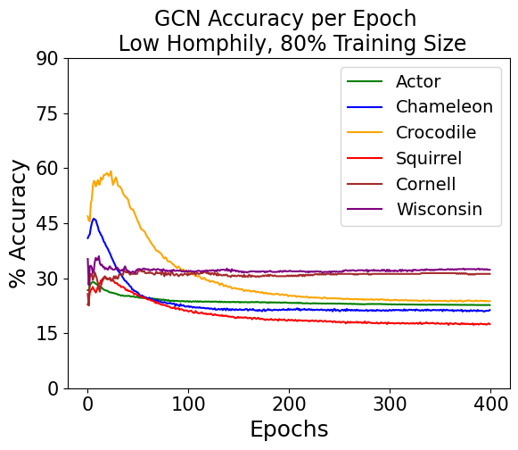
(a)

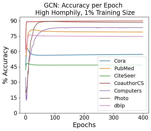
(b)

Figure 3: These figures provide the test set performance for the tuned GCN model on each dataset for medium difficulty graph complexity and training conditions. Plots for GATv2 and GraphSAGE look similar.

5.2.3 Adjusting the number of layers and other hyperparameters

GNNs have many design variables in addition to their hidden dimensions. We use the results of You et al. [104] to decide which design variables to focus on. Our fixed design variables are listed in Table 7, and we investigate how performance changes by tuning the other six, given in Table 8. You et al. [104] provide performance rankings of hyperparameter configurations but no information on their contributions to improving the evaluation metric score, so we address this question for node classification.

Table 7: Hyperparameter values shared by top performing designs in You et al. [104].

Parameter Value Parameter Value Activation PReLU Batch Size 32 Batch Norm True Optimizer Adam Dropout False Epochs 400

Table 8: Hyperparameter values to tune

Tuning Parameter Order Starting Value Options Message-Passing Layers 1 2 1, 2, 3, 4, 5, 6, 7, 8 Post-Processing Layers 2 1 1, 2, 3 Pre-Processing Layers 3 1 1, 2, 3 Layer Connectivity 4 Skip Sum None, Skip Sum, Skip Concatenate Aggregation Function 5 Mean Add, Mean, Max Learning Rate 6 0.01 0.005, 0.01, 0.0125, 0.015

We choose each option from Table 8 in a greedy fashion, by first finding the best option for the number of message-passing layers and then proceeding according to the tuning order in the table. All models are trained for 400 epochs. Every dataset is partitioned between training and test sets, and the best hyperparameter selection is the one with the highest average test set accuracy from 25 experiments. Following You et al. [104], we adjust the number of hidden layers to make the size of each design comparable, and thus enable a fair comparison of them.

Table 9: The average improvement of node classification accuracy for the tuned designs over the default design with 128 hidden dimensions (see Section 5.2.1) on high and low dataset collections, with 1% and 80% of node labels for training. The hyperparameters for each algorithm have been tuned to each dataset.

Average Node Classification Accuracy Improvement over Default with 128 Hidden Dims 80% Training 80% Training 1% Training 1% Training Model Name High Homophily Low Homophily High Homophily Low Homophily (Difficulty) (Easy) (Medium) (Medium) (Hard) GCN +0.57 +22.98 +0.93 $-0.22$ GATv2 +1.53 +16.39 +4.57 $-0.92$ GraphSAGE +0.15 +6.18 +4.02 $-3.89$

Table 9 shows there is little or no value in tuning the structure of the GNN to the dataset in the easy or hard conditions. In fact, the off-the-shelf models outperform the hyperparameter tuned ones in the hard condition. This may be due to starting from a suboptimal design compared to the design chosen by the architecture creators, and additionally there being little benefit to tuning any individual hyperparameter selection beyond that.

The most benefit for tuning the GNN design occurs when the training and dataset conditions are of medium difficulty. Although the tuned GraphSAGE performs best on low homophily graphs and the tuned GCN performs best on high homophily ones, once tuned, all models perform comparably. Table 10 indicates that most of the gain on the low homophily graphs with plenty of training data comes from the Cornell and Wisconsin datasets. Cornell and Wisconsin are special in that they are small datasets with low homophily and a high SNR among their node features. Having fewer nodes may have made the GNN performance more sensitive to improvements, and the datasets having a high SNR may have enabled a reasonably high node classification accuracy, with the appropriate hyperparameter configuration.

Table 10: The average improvement of node classification accuracy for tuned designs over default ones with 128 hidden dimensions (see Section 5.2.1) on the collection of Cornell and Wisconsin datasets versus the collection of other low homophily datasets, with 80% of nodes training. The hyperparameters for each algorithm have been tuned to each dataset.

Node Classification Accuracy Improvement 80% Training Cornell & Wisconsin Other Low Homophily GCN +49.32 +9.37 GATv2 +41.58 +3.80 GraphSAGE +22.89 $-2.12$

The following sections analyze hyperparameter configurations from the medium difficulty conditions.

Hyperparameter selection for improved node classification accuracy

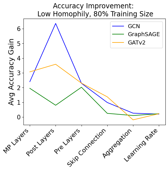
(a)

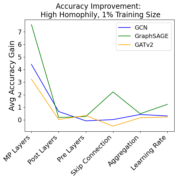
(b)

Figure 4: Following the greedy hyperparameter tuning process described in Section 5.2.3, the figures show the improved node classification accuracy after tuning the given design component of the GNN compared to the design before it was tuned.

Table 11: The mean value and $p$-value of the number of layers and the learning rates of the hyperparameter tuned models. The hyperparemeters were tuned for each model on the low and high homophily dataset collections with 1% and 80% of node labels for training. For each hyperparameter, the $p$-value is for the null hypothesis that the selections over the collection of datasets are drawn from a random distribution.

Statistics of Design Parameters of Tuned GNNs 80% Training Pre Layers MP Layers Post Layers LR Low Homophily mean $p$-value mean $p$-value mean $p$-value mean $p$-value GCN $2.17$ $0.23$ $3.67$ $0.21$ $3.0$ $0.0$ $0.024$ $0.0$ GATv2 $2.0$ $0.41$ $3.83$ $0.27$ $2.83$ $0.0$ $0.012$ $0.17$ GraphSAGE $1.83$ $0.4$ $6.5$ $0.01$ $2.17$ $0.23$ $0.011$ $0.34$ 1% Training High Homophily GCN $1.57$ $0.12$ $6.86$ $0.0$ $1.43$ $0.05$ $0.010\phantom{0}$ $0.37$ GATv2 $1.71$ $0.25$ $5.86$ $0.05$ $1.43$ $0.05$ $0.010\phantom{0}$ $0.46$ GraphSAGE $2.29$ $0.13$ $7.71$ $0.0$ $1.71$ $0.25$ $0.0075$ $0.02$

Table 12: The most common and % occurring values of the skip connections and aggregation functions on the low and high homophily dataset collections, with 1% and 80% of nodes training. The hyperparameters for the algorithms have been tuned to each dataset. The % occurring field says how often the most common selection occurred.

Statistics of Design Parameters of Tuned GNNs 80% Training Skip Connections Aggregation Low Homophily most common % occurring most common % occurring GCN skip concat $66.67$ max $50.0\phantom{0}$ GATv2 skip concat $100.0\phantom{0}$ add $50.0\phantom{0}$ GraphSAGE skip sum $66.67$ add $66.67$ 1% Training High Homophily GCN skip sum $71.43$ max $71.43$ GATv2 skip sum $100.0\phantom{0}$ max $57.14$ GraphSAGE none $71.43$ add $42.86$

Figure 4 shows the improvement due to each hyperparameter relative to the design before that hyperparameter was tuned. We see that the number of message-passing layers is the most important hyperparameter to tune on high homophily graphs, and Table 11 shows that a larger number of message-passing layers is best. (In Section 5.3, we provide a qualitative description of this when we evaluate how node features separate among classes). This preference is reinforced from there being fewer training data because deeper networks have a larger receptive field.

In contrast, Figure 4 shows that a broader collection of parameters could be profitably tuned to improve performance on low homophily graphs. On low homophily graphs, aggregating over neighborhoods produces a signal from conflicting information, so we should expect that the number of message-passing layers in the tuned networks would be lower. It is somewhat surprising that message-passing layers are helpful at all, but we see that having some message-passing layers tends to significantly outperform the node feature-only model, MLP. GNNs on these graphs tend to have higher numbers of pre- and post-processing layers, which helps to tune the features according to the node’s class, independent of their neighbors’ features.

The importance of skip connections is hard to determine from Figure 4 alone. Figure 4 shows little improvement for a given model and component, it is not clear whether this is because the starting design is the best selection or the component has little impact on performance. To answer this, Tables 11 and 12 inform the statistical likelihood of getting the results by random chance. For example, the starting designs all use skip sum connections. Figure 4 indicates that this option is not important for improving GATv2 performance in the 1% training and high homophily configuration, but Tables 11 and 12 show that skip sums are the top selection for GATv2 every time. This means that skip connections are important and skip sum is the best option for GATv2. On the other hand, Figure 4 and Table 12 show GraphSAGE performance tends to be best without skip connections on high homophily graphs. GraphSAGE already has a skip connection from its function $\bigwedge$ being concatenation, so it apparently does not need another one.

Tuning the remaining hyperparameters appears to have relatively little effect.

Node classification accuracy per training epoch, again

Recall that Figure 3(a) shows a sharp decrease in performance at around 25 epochs for several low homophily datasets. After tuning the other hyperparameters, Figure 5(b) shows that node classification accuracy generally stabilizes and improves for these datasets, like they do for the high homophily graphs. We hypothesize that the extra processing provided by pre- and post-processing layers without neighborhood node feature information is especially beneficial for this.

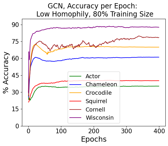
(a)

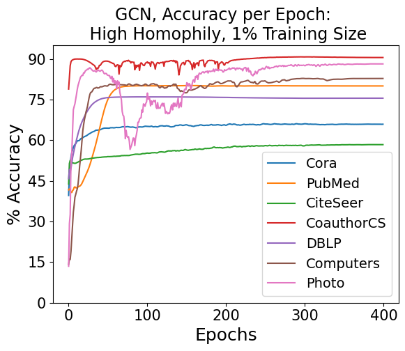
(b)

Figure 5: These figures provide the test set performance for the tuned GCN model on each dataset for the medium difficulty conditions. Plots for the GATv2 and GraphSAGE models look the similar.

Comparison with top-performing off-the-shelf GNNs

For context, we compare these results with a class of models called RevGNNs that are used in models toward the top of the leaderboard on node classification datasets of Open Graph Benchmark. RevGNNs provide us ground truth for “good” node classification performance for comparison. They are built on top of the GCN, GAT or GraphSAGE encoders, and are designed in a way that makes computations independent of the depth of the network [99]. This means they can be arbitrarily deep without running out of memory, although training time increases. We apply the RevGNNs in an off-the-shelf manner. All RevGNNs have 160 hidden dimensions, and 4 layers, and they were trained for 200 epochs, using an 80/10/10 train/val/test split. Tables 13 shows the hyperparameter tuned GNNs perform comparably or outperform the off-the-shelf RevGNNs.

Table 13: Node classification accuracy comparison of models on low and high homophily dataset collections, with 1% and 80% of node labels for training.

Node Classification Accuracy 80% Training 1% Training Model Name Low Homophily High Homophily GCN-128 39.34 76.46 GCN${}_{\textrm{Tuned}}$ 62.32 77.39 RevGCN 50.93 77.86 GATv2-128 45.55 72.14 GATv2${}_{\textrm{Tuned}}$ 61.94 76.71 RevGATv2 53.64 77.99 GraphSAGE-128 57.27 71.89 GraphSAGE${}_{\textrm{Tuned}}$ 63.45 75.91 RevSAGE 59.61 75.87

5.3 Qualitative description of GNN learning

Recall from Section 4.1 that each layer of the GNN transforms the node feature vectors into new feature vectors that are inputs to the next layer. Figure 6 describes the energy of the signal and noise (defined in Equation (58)) at each epoch in the final hidden layer of each model. As the number of training epochs gets larger, the energy of the noise stays flat while that of the signal gets larger, which means that node feature vectors generally separate between classes while their within-class variance stays the same. In contrast, experiments show that MLP performance does not improve after around 100 epochs, as indicated in Figures 6(c) and 6(d).

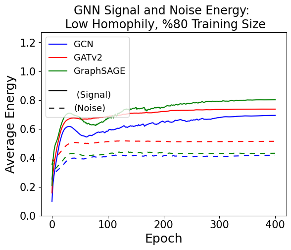
(a)

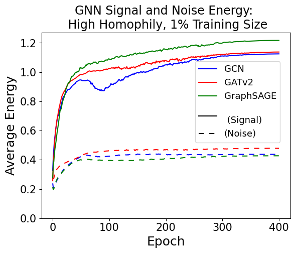
(b)

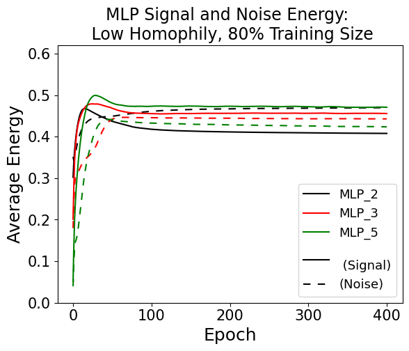
(c)

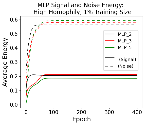
(d)

Figure 6: These figures show the energy of the signal and the noise for each model, averaged over all datasets in each medium difficulty case.

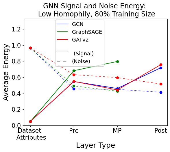
(a)

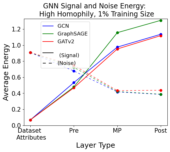
(b)

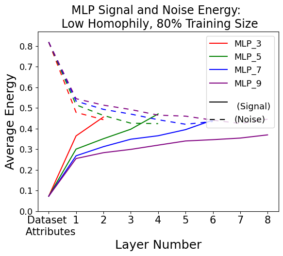
(c)

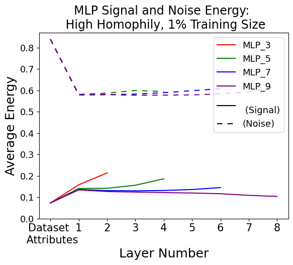
(d)

Figure 7: These figures show the energy of the signal and the noise in the final hidden layer of each layer type. For some of the low homophily datasets, the tuned GraphSAGE design has no hidden post-processing layers, so the plot does not include the post-processing layers for this model.

Di Giovanni et al. [107] mathematically analyze an energy potential as it passes through the message-passing layers, where the potential concerns the energies of the node feature signal and noise. Figures 7(a) and 7(b) experimentally illustrate signal and noise energies as node features pass through all layer types. The noise drops significantly in the pre-processing layers. In the high homophily case, the noise drops again in the message-passing layers. This is intuitive because the message-passing layers aggregate information from their neighboring nodes, which tend to have the same class label and similar node features. This brings together similar node features, reducing the node feature noise. Figures 7(c) and 7(d) show what happens when the message-passing layer is removed. Here, there are MLP models with a comparable number of layers to what we have in tuned GNNs, but the noise of the node features is flat.

GNNs do not get the same advantage on low homophily graphs because neighboring nodes tend to be of different classes so their features have different information. This makes node features from different classes more similar. Consistent with this, the energy of the signal in GCN and GATv2 is smaller after the message-passing step in Figure 7(b). Only the energy of the signal for GraphSAGE is larger following the message-passing layers. GraphSAGE’s use of concatenation for the function $\bigwedge$ explains this. Concatenation allows it to learn on each node’s feature vector directly instead of first mixing with the aggregate of its neighbors’ vectors, so the node features can more easily separate by class.

Message-passing layers in a GNN provide node features with information from the neighbors, and then post-processing layers further refine the embeddings, leading to further separation of the classes. Notice from Figures 7(c) and 7(d) that MLP models do not benefit from having more than three layers.

6 Conclusion

A decade ago deep convolutional neural networks for image classification initiated a revolution where feature learning was integrated into the training process of a neural network, and this was subsequently extended to data structures like irregular graphs. The encoder-decoder framework neatly describes these models, and the shortcomings of simpler encoder-decoder models motivates the use of more complicated Graph Neural Networks (GNNs). Graph neural networks have attracted considerable attention due to state-of-the-art results on a range of graph analysis tasks and datasets, but because of the great variety of graphs and graph analysis tasks, they can be difficult to use for those new to the field. As such, we hope our overview of GNNs, their construction and behavior on a variety of datasets and training conditions, has prepared the reader to solve diverse graph problems and understand the technical aspects of literature.

Appendix A Open-source GNN libraries

To our knowledge, PyTorch Geometric and Deep Graph Library are the largest and most widely used libraries.

• PyTorch Geometric

  This library is built on PyTorch and its design aims to stay close to usual PyTorch [108]. It provides well-documented examples, and benchmark datasets and most state-of-the art GNN models are available here. Many GNNs from the literature are implemented, and it supports multi-GPU processing.

• Deep Graph Library

  This library is sponsored by AWS, NSF, NVIDIA and Intel [109]. It supports multi-GPU processing and the PyTorch, TensorFlow and Apache MXNet frameworks. They have well-documented examples and example code for many state-of-the art models.

• GeometricFlux.jl

  This is a Julia library for geometric deep learning [110], as described in [4]. It supports deep learning in a range of settings: Graphs and sets; grids and Euclidean spaces; groups and homogeneous spaces; geodesics and manifolds; gauges and bundles. It also offers GPU support and has integration with GNN benchmark datasets. It supports both graph network architectures, which are more general graph models than graph neural networks [1], and message-passing architectures.

• Spektral

  This library is built on TensorFlow 2 and Keras [111]. It intends to feel close to the Keras API and to be flexible and easy to use. It provides code for the standard components of GNNs as well as example implementations of GNNs on specific datasets.

• Jraph

  This is a library written in JAX, which is a language that enables automatic differentiation of python and numpy. It is created by DeepMind and inherits some design properties from its earlier library, Graph Nets. Like Graph Nets, it supports building graph networks and is a lightweight library with utilities for working with graphs. Unlike Graph Nets, it has a model zoo of graph neural network models.

• Graph Nets

  This is a DeepMind library in TensorFlow and Sonnet library for building graph networks as described in [1]. It supports both CPU and GPU processing, but as of this writing, it is not actively maintained.

• Stellar Graph

  This library is built on TensorFlow 2 and uses the Keras API. It supports a variety of graph machine learning tasks including node classification, link prediction and graph classification on a homogeneous graphs, heterogeneous graphs and other graph types. As of this writing, it is not actively maintained.

• PyTorch GNN

  This Microsoft library is written in PyTorch and is primarily engineered to be fast on sparse graphs. Graph neural network models from several papers and graph analysis tasks are implemented. This library is not actively maintained as of this writing.

Appendix B Results on Individual Datasets

All tables report results with 95% confidence intervals.

Table 14: The node classification accuracy of default designs (see Table 4).

Node Classification Accuracy: 80% Training and 16 Hidden Dimensions Dataset GCN GATv2 GraphSAGE Photo 89.48 $\pm$ 3.47 93.55 $\pm$ 0.37 77.95 $\pm$ 8.99 DBLP 85.16 $\pm$ 0.29 85.11 $\pm$ 0.32 84.84 $\pm$ 0.30 Cora 88.28 $\pm$ 0.74 85.71 $\pm$ 0.79 88.25 $\pm$ 0.66 CoauthorCS 93.22 $\pm$ 0.21 91.24 $\pm$ 0.29 94.26 $\pm$ 0.21 PubMed 87.21 $\pm$ 0.24 86.99 $\pm$ 0.26 87.89 $\pm$ 0.38 Computers 77.34 $\pm$ 5.09 89.88 $\pm$ 0.39 77.45 $\pm$ 5.16 CiteSeer 76.46 $\pm$ 0.93 76.19 $\pm$ 0.88 75.77 $\pm$ 1.03 Crocodile 61.66 $\pm$ 0.96 68.26 $\pm$ 0.69 73.26 $\pm$ 0.44 Chameleon 46.90 $\pm$ 1.17 55.34 $\pm$ 1.39 64.07 $\pm$ 1.30 Squirrel 29.53 $\pm$ 1.07 37.68 $\pm$ 0.73 45.24 $\pm$ 0.70 Cctor 27.66 $\pm$ 0.68 28.89 $\pm$ 0.65 35.08 $\pm$ 0.64 Wisconsin 32.00 $\pm$ 3.30 40.00 $\pm$ 2.80 66.31 $\pm$ 4.05 Cornell 28.42 $\pm$ 2.80 39.16 $\pm$ 3.25 56.21 $\pm$ 4.11

Table 15: The node classification accuracy of default designs (see Table 4).

Node Classification Accuracy: 1% Training and 16 Hidden Dimensions Dataset GCN GATv2 GraphSAGE Photo 78.35 $\pm$ 7.05 78.71 $\pm$ 1.81 65.22 $\pm$ 5.18 DBLP 74.80 $\pm$ 0.69 74.63 $\pm$ 0.89 72.50 $\pm$ 0.96 Cora 60.55 $\pm$ 2.78 54.89 $\pm$ 2.78 55.93 $\pm$ 1.52 CoauthorCS 89.94 $\pm$ 0.22 77.13 $\pm$ 0.79 86.10 $\pm$ 0.36 PubMed 81.16 $\pm$ 0.37 79.14 $\pm$ 0.46 78.86 $\pm$ 0.33 Computers 74.83 $\pm$ 4.76 72.64 $\pm$ 1.63 54.20 $\pm$ 4.22 CiteSeer 48.38 $\pm$ 1.70 48.74 $\pm$ 2.26 43.70 $\pm$ 1.88 Crocodile 46.44 $\pm$ 1.58 45.38 $\pm$ 1.67 52.91 $\pm$ 1.30 Chameleon 30.58 $\pm$ 1.59 30.56 $\pm$ 1.35 31.47 $\pm$ 1.77 Squirrel 22.16 $\pm$ 0.57 22.39 $\pm$ 0.66 26.93 $\pm$ 1.08 Cctor 24.44 $\pm$ 0.38 23.98 $\pm$ 0.49 24.48 $\pm$ 0.62 Wisconsin 34.03 $\pm$ 5.74 38.60 $\pm$ 4.18 40.22 $\pm$ 4.83 Cornell 28.26 $\pm$ 5.58 24.65 $\pm$ 5.56 29.96 $\pm$ 5.05

Table 16: The node classification accuracy of default designs (see Table 6).

Node Classification Accuracy: 80% Training and 32 Hidden Dimensions Dataset GCN GATv2 GraphSAGE Photo 93.45 $\pm$ 0.40 93.46 $\pm$ 0.35 91.68 $\pm$ 3.23 DBLP 85.85 $\pm$ 0.35 85.15 $\pm$ 0.35 84.94 $\pm$ 0.45 Cora 88.84 $\pm$ 0.48 86.65 $\pm$ 0.95 88.35 $\pm$ 0.63 CoauthorCS 93.20 $\pm$ 0.26 91.61 $\pm$ 0.38 94.36 $\pm$ 0.25 PubMed 87.51 $\pm$ 0.25 86.97 $\pm$ 0.31 88.16 $\pm$ 0.29 Computers 88.49 $\pm$ 0.56 90.15 $\pm$ 0.35 83.45 $\pm$ 4.05 CiteSeer 77.49 $\pm$ 0.90 75.63 $\pm$ 0.96 75.96 $\pm$ 0.90 Crocodile 62.01 $\pm$ 0.79 68.76 $\pm$ 0.69 72.79 $\pm$ 0.55 Chameleon 46.52 $\pm$ 1.19 54.53 $\pm$ 1.48 64.59 $\pm$ 1.58 Squirrel 29.60 $\pm$ 1.00 38.17 $\pm$ 0.89 44.64 $\pm$ 0.77 Cctor 28.22 $\pm$ 0.78 29.06 $\pm$ 0.72 35.23 $\pm$ 0.66 Wisconsin 32.62 $\pm$ 3.05 40.46 $\pm$ 2.93 67.08 $\pm$ 3.05 Cornell 29.26 $\pm$ 2.98 39.37 $\pm$ 4.67 59.79 $\pm$ 3.73

Table 17: The node classification accuracy of default designs (see Table 6).

Node Classification Accuracy: 1% Training and 32 Hidden Dimensions Dataset GCN GATv2 GraphSAGE Photo 88.67 $\pm$ 0.74 81.73 $\pm$ 1.60 77.02 $\pm$ 3.34 DBLP 75.93 $\pm$ 0.69 75.32 $\pm$ 0.60 73.60 $\pm$ 0.75 Cora 63.57 $\pm$ 2.02 59.40 $\pm$ 2.53 56.16 $\pm$ 2.20 CoauthorCS 89.90 $\pm$ 0.25 80.23 $\pm$ 0.74 86.97 $\pm$ 0.46 PubMed 80.94 $\pm$ 0.43 79.10 $\pm$ 0.53 79.23 $\pm$ 0.36 Computers 82.05 $\pm$ 1.44 75.01 $\pm$ 1.26 64.95 $\pm$ 3.38 CiteSeer 49.90 $\pm$ 2.22 49.88 $\pm$ 2.31 47.79 $\pm$ 2.66 Crocodile 46.59 $\pm$ 1.74 47.85 $\pm$ 1.78 52.64 $\pm$ 0.90 Chameleon 31.42 $\pm$ 1.55 29.48 $\pm$ 1.21 31.61 $\pm$ 1.56 Squirrel 22.95 $\pm$ 0.40 22.46 $\pm$ 0.58 28.08 $\pm$ 0.71 Cctor 24.46 $\pm$ 0.50 24.03 $\pm$ 0.51 25.50 $\pm$ 0.47 Wisconsin 34.98 $\pm$ 5.18 36.60 $\pm$ 4.74 38.00 $\pm$ 5.26 Cornell 27.91 $\pm$ 5.23 24.00 $\pm$ 5.30 32.30 $\pm$ 5.78

Table 18: The node classification accuracy of default designs (see Table 6).

Node Classification Accuracy: 80% Training and 64 Hidden Dimensions Dataset GCN GATv2 GraphSAGE Photo 93.69 $\pm$ 0.26 93.54 $\pm$ 0.36 94.24 $\pm$ 0.54 DBLP 85.69 $\pm$ 0.31 85.03 $\pm$ 0.26 84.72 $\pm$ 0.36 Cora 88.69 $\pm$ 0.70 86.10 $\pm$ 0.78 88.59 $\pm$ 0.68 CoauthorCS 93.48 $\pm$ 0.20 92.04 $\pm$ 0.33 94.69 $\pm$ 0.16 PubMed 87.64 $\pm$ 0.29 87.27 $\pm$ 0.39 88.23 $\pm$ 0.36 Computers 88.96 $\pm$ 0.42 90.27 $\pm$ 0.31 88.83 $\pm$ 0.75 CiteSeer 77.09 $\pm$ 0.82 75.68 $\pm$ 0.96 75.95 $\pm$ 0.68 Crocodile 63.46 $\pm$ 0.75 68.93 $\pm$ 0.50 73.05 $\pm$ 0.37 Chameleon 47.48 $\pm$ 1.72 56.16 $\pm$ 1.23 64.21 $\pm$ 0.97 Squirrel 30.20 $\pm$ 0.72 38.50 $\pm$ 0.87 44.85 $\pm$ 0.77 Cctor 28.59 $\pm$ 0.57 28.37 $\pm$ 0.85 34.87 $\pm$ 0.65 Wisconsin 36.62 $\pm$ 2.83 38.92 $\pm$ 3.82 68.62 $\pm$ 3.29 Cornell 28.63 $\pm$ 4.13 40.00 $\pm$ 4.25 61.89 $\pm$ 4.01

Table 19: The node classification accuracy of default designs (see Table 6).

Node Classification Accuracy: 1% Training and 64 Hidden Dimensions Dataset GCN GATv2 GraphSAGE Photo 89.13 $\pm$ 0.69 81.97 $\pm$ 1.02 80.10 $\pm$ 1.56 DBLP 76.01 $\pm$ 0.50 75.08 $\pm$ 0.94 73.99 $\pm$ 0.65 Cora 62.96 $\pm$ 2.78 61.57 $\pm$ 2.32 58.48 $\pm$ 2.77 CoauthorCS 89.81 $\pm$ 0.26 80.42 $\pm$ 0.75 86.80 $\pm$ 0.55 PubMed 80.98 $\pm$ 0.40 79.66 $\pm$ 0.42 79.14 $\pm$ 0.38 Computers 83.09 $\pm$ 0.49 76.20 $\pm$ 0.81 71.25 $\pm$ 3.31 CiteSeer 51.01 $\pm$ 1.87 49.99 $\pm$ 2.21 50.67 $\pm$ 2.07 Crocodile 46.40 $\pm$ 1.59 47.51 $\pm$ 1.30 53.96 $\pm$ 0.65 Chameleon 31.84 $\pm$ 1.19 30.03 $\pm$ 1.80 33.39 $\pm$ 1.38 Squirrel 22.66 $\pm$ 0.62 22.84 $\pm$ 0.57 27.80 $\pm$ 0.82 Cctor 23.26 $\pm$ 0.80 23.91 $\pm$ 0.66 24.78 $\pm$ 0.54 Wisconsin 38.32 $\pm$ 4.71 33.56 $\pm$ 4.93 41.40 $\pm$ 5.31 Cornell 29.26 $\pm$ 6.03 25.09 $\pm$ 5.55 33.26 $\pm$ 6.12

Table 20: The node classification accuracy of default designs (see Table 6).

Node Classification Accuracy: 80% Training and 128 Hidden Dimensions Dataset GCN GATv2 GraphSAGE Photo 93.87 $\pm$ 0.32 93.21 $\pm$ 0.29 95.24 $\pm$ 0.37 DBLP 85.69 $\pm$ 0.34 85.33 $\pm$ 0.26 84.89 $\pm$ 0.22 Cora 88.81 $\pm$ 0.65 85.97 $\pm$ 0.72 88.29 $\pm$ 0.70 CoauthorCS 93.49 $\pm$ 0.20 92.34 $\pm$ 0.29 94.73 $\pm$ 0.20 PubMed 88.19 $\pm$ 0.34 87.31 $\pm$ 0.29 88.65 $\pm$ 0.29 Computers 90.23 $\pm$ 0.31 90.27 $\pm$ 0.34 89.96 $\pm$ 0.51 CiteSeer 76.91 $\pm$ 0.88 76.19 $\pm$ 0.93 76.80 $\pm$ 0.94 Crocodile 63.13 $\pm$ 0.53 69.28 $\pm$ 0.67 73.42 $\pm$ 0.60 Chameleon 47.06 $\pm$ 1.88 54.46 $\pm$ 1.33 64.14 $\pm$ 1.34 Squirrel 29.16 $\pm$ 0.85 39.45 $\pm$ 0.88 45.02 $\pm$ 0.73 Cctor 28.42 $\pm$ 0.66 29.06 $\pm$ 0.48 35.15 $\pm$ 0.54 Wisconsin 36.92 $\pm$ 3.25 40.62 $\pm$ 3.28 68.00 $\pm$ 2.95 Cornell 31.37 $\pm$ 3.48 40.42 $\pm$ 4.20 57.89 $\pm$ 3.40

Table 21: The node classification accuracy of default designs (see Table 6).

Node Classification Accuracy: 1% Training and 128 Hidden Dimensions Dataset GCN GATv2 GraphSAGE Photo 89.57 $\pm$ 0.63 81.27 $\pm$ 0.94 80.39 $\pm$ 1.61 DBLP 76.43 $\pm$ 0.69 75.21 $\pm$ 0.71 74.24 $\pm$ 0.54 Cora 64.08 $\pm$ 2.31 60.72 $\pm$ 2.97 58.55 $\pm$ 2.20 CoauthorCS 89.76 $\pm$ 0.24 81.40 $\pm$ 0.84 86.25 $\pm$ 0.50 PubMed 81.06 $\pm$ 0.33 79.19 $\pm$ 0.36 79.54 $\pm$ 0.28 Computers 83.53 $\pm$ 0.50 75.27 $\pm$ 1.04 72.91 $\pm$ 2.27 CiteSeer 50.80 $\pm$ 1.88 51.95 $\pm$ 1.86 51.30 $\pm$ 2.08 Crocodile 46.90 $\pm$ 1.72 47.44 $\pm$ 2.25 54.55 $\pm$ 0.85 Chameleon 31.24 $\pm$ 1.63 30.40 $\pm$ 1.36 34.75 $\pm$ 1.59 Squirrel 23.46 $\pm$ 0.51 22.36 $\pm$ 0.67 28.84 $\pm$ 0.77 Cctor 24.11 $\pm$ 0.64 23.71 $\pm$ 0.62 25.15 $\pm$ 0.45 Wisconsin 33.30 $\pm$ 5.34 36.13 $\pm$ 5.30 34.29 $\pm$ 5.57 Cornell 28.61 $\pm$ 5.98 31.30 $\pm$ 5.87 36.30 $\pm$ 4.84

Table 22: The node classification accuracy of default designs (see Table 6).

Node Classification Accuracy: 80% Training and 256 Hidden Dimensions Dataset GCN GATv2 GraphSAGE Photo 93.77 $\pm$ 0.24 93.46 $\pm$ 0.37 94.94 $\pm$ 0.30 DBLP 85.33 $\pm$ 0.33 84.78 $\pm$ 0.38 84.78 $\pm$ 0.36 Cora 88.13 $\pm$ 1.00 86.69 $\pm$ 0.79 88.35 $\pm$ 0.91 CoauthorCS 93.37 $\pm$ 0.28 92.34 $\pm$ 0.33 94.57 $\pm$ 0.20 PubMed 88.31 $\pm$ 0.30 87.10 $\pm$ 0.26 88.52 $\pm$ 0.21 Computers 90.33 $\pm$ 0.36 90.06 $\pm$ 0.35 90.56 $\pm$ 0.32 CiteSeer 76.59 $\pm$ 0.66 75.02 $\pm$ 1.00 76.40 $\pm$ 0.96 Crocodile 64.04 $\pm$ 0.66 69.49 $\pm$ 0.54 73.29 $\pm$ 0.51 Chameleon 47.13 $\pm$ 1.35 56.14 $\pm$ 1.35 63.44 $\pm$ 1.21 Squirrel 29.07 $\pm$ 0.62 38.93 $\pm$ 0.85 45.93 $\pm$ 0.76 Cctor 28.13 $\pm$ 0.56 28.71 $\pm$ 0.70 35.62 $\pm$ 0.60 Wisconsin 34.92 $\pm$ 3.49 38.46 $\pm$ 3.25 68.77 $\pm$ 2.77 Cornell 30.11 $\pm$ 3.33 39.58 $\pm$ 5.06 56.84 $\pm$ 3.20

Table 23: The node classification accuracy of default designs (see Table 6).

Node Classification Accuracy: 1% Training and 256 Hidden Dimensions Dataset GCN GATv2 GraphSAGE Photo 89.08 $\pm$ 0.69 78.98 $\pm$ 1.62 81.93 $\pm$ 1.45 DBLP 76.65 $\pm$ 0.61 75.29 $\pm$ 0.93 74.45 $\pm$ 0.52 Cora 66.21 $\pm$ 2.31 62.17 $\pm$ 2.59 61.51 $\pm$ 1.83 CoauthorCS 89.64 $\pm$ 0.23 81.75 $\pm$ 1.28 84.78 $\pm$ 0.98 PubMed 81.21 $\pm$ 0.33 79.07 $\pm$ 0.44 79.39 $\pm$ 0.37 Computers 83.59 $\pm$ 0.56 72.81 $\pm$ 0.88 74.99 $\pm$ 1.95 CiteSeer 52.50 $\pm$ 2.28 50.94 $\pm$ 2.04 52.20 $\pm$ 1.44 Crocodile 47.64 $\pm$ 1.37 46.73 $\pm$ 1.63 54.07 $\pm$ 0.73 Chameleon 30.94 $\pm$ 1.69 32.71 $\pm$ 1.38 33.91 $\pm$ 1.35 Squirrel 23.23 $\pm$ 0.53 22.62 $\pm$ 0.54 28.52 $\pm$ 0.83 Cctor 24.67 $\pm$ 0.42 24.42 $\pm$ 0.61 25.73 $\pm$ 0.55 Wisconsin 36.22 $\pm$ 5.71 33.43 $\pm$ 5.22 40.16 $\pm$ 5.84 Cornell 27.91 $\pm$ 5.30 25.09 $\pm$ 6.26 24.39 $\pm$ 5.77

Table 24: The node classification accuracy of the tuned designs with 80% of nodes labeled for training (see Table 9).

Node Classification Accuracy with 80% Training Dataset GCN_tuned GraphSAGE_tuned GATv2_tuned Photo 95.62 $\pm$ 0.18 95.68 $\pm$ 0.16 95.65 $\pm$ 0.18 DBLP 84.86 $\pm$ 0.18 84.59 $\pm$ 0.22 84.89 $\pm$ 0.17 Cora 88.00 $\pm$ 0.49 87.81 $\pm$ 0.47 88.26 $\pm$ 0.46 CoauthorCS 95.36 $\pm$ 0.12 95.17 $\pm$ 0.14 95.17 $\pm$ 0.13 PubMed 90.04 $\pm$ 0.22 89.89 $\pm$ 0.16 89.99 $\pm$ 0.21 Computers 91.95 $\pm$ 0.16 91.56 $\pm$ 0.18 91.95 $\pm$ 0.15 CiteSeer 75.35 $\pm$ 0.62 74.88 $\pm$ 0.49 75.41 $\pm$ 0.48 Crocodile 70.31 $\pm$ 0.36 70.31 $\pm$ 0.34 70.74 $\pm$ 0.34 Chameleon 61.20 $\pm$ 0.80 61.01 $\pm$ 0.78 60.66 $\pm$ 0.82 Squirrel 40.29 $\pm$ 0.62 42.23 $\pm$ 0.59 40.79 $\pm$ 0.68 Actor 35.19 $\pm$ 0.47 35.68 $\pm$ 0.36 35.26 $\pm$ 0.46 Wisconsin 87.37 $\pm$ 1.66 89.73 $\pm$ 1.80 87.45 $\pm$ 2.36 Cornell 79.57 $\pm$ 2.29 81.95 $\pm$ 2.00 76.76 $\pm$ 1.99

Table 25: The node classification accuracy of tuned designs with 1% of nodes labeled for training (see Table 9).

Node Classification Accuracy with 1% Training Dataset GCN_tuned GraphSAGE_tuned GATv2_tuned Photo 88.71 $\pm$ 0.68 85.98 $\pm$ 0.87 87.96 $\pm$ 0.78 DBLP 75.51 $\pm$ 0.60 73.75 $\pm$ 0.74 75.64 $\pm$ 0.60 Cora 66.62 $\pm$ 1.52 66.65 $\pm$ 2.15 63.53 $\pm$ 2.16 CoauthorCS 90.60 $\pm$ 0.43 89.59 $\pm$ 0.60 90.52 $\pm$ 0.22 PubMed 79.71 $\pm$ 0.40 78.06 $\pm$ 0.43 79.50 $\pm$ 0.45 Computers 82.54 $\pm$ 0.50 82.08 $\pm$ 0.80 83.51 $\pm$ 0.51 CiteSeer 58.01 $\pm$ 1.50 55.32 $\pm$ 1.94 56.32 $\pm$ 1.45 Crocodile 56.12 $\pm$ 0.78 57.02 $\pm$ 0.76 55.54 $\pm$ 0.60 Chameleon 33.46 $\pm$ 1.39 33.42 $\pm$ 1.22 33.52 $\pm$ 1.38 Squirrel 25.88 $\pm$ 0.59 27.70 $\pm$ 0.70 25.80 $\pm$ 0.47 Actor 25.65 $\pm$ 0.35 25.82 $\pm$ 0.51 25.66 $\pm$ 0.45 Wisconsin 27.93 $\pm$ 0.08 27.69 $\pm$ 0.42 27.69 $\pm$ 0.45 Cornell 17.25 $\pm$ 1.23 18.90 $\pm$ 1.52 17.52 $\pm$ 1.30

Table 26: The node classification accuracy of RevGNNs with 80% of node labels for training on low homophily graphs (see Table 13).

Node Classification Accuracy of RevGNNs Dataset RevGCN RevSAGE RevGATv2 Crocodile 69.01 $\pm$ 0.55 73.10 $\pm$ 0.53 71.36 $\pm$ 0.54 Chameleon 54.60 $\pm$ 1.18 64.10 $\pm$ 1.36 60.00 $\pm$ 1.49 Squirrel 36.25 $\pm$ 0.90 46.34 $\pm$ 1.07 42.63 $\pm$ 0.80 Actor 33.29 $\pm$ 0.61 36.91 $\pm$ 0.73 36.22 $\pm$ 0.67 Wisconsin 61.38 $\pm$ 3.50 71.08 $\pm$ 2.73 63.85 $\pm$ 3.28 Cornell 51.16 $\pm$ 4.06 66.11 $\pm$ 2.80 47.79 $\pm$ 2.91

Table 27: The node classification accuracy of RevGNNs with 1% of node labels for training on high homophily graphs (see Table 13).

Node Classification Accuracy of RevGNNs Dataset RevGCN RevSAGE RevGATv2 Photo 88.89 $\pm$ 0.86 87.12 $\pm$ 0.81 90.21 $\pm$ 0.54 DBLP 77.73 $\pm$ 0.69 76.21 $\pm$ 0.72 77.71 $\pm$ 0.68 Cora 67.37 $\pm$ 1.63 62.41 $\pm$ 2.03 67.96 $\pm$ 1.94 CoauthorCS 91.59 $\pm$ 0.34 90.72 $\pm$ 0.29 90.86 $\pm$ 0.34 PubMed 81.83 $\pm$ 0.39 79.98 $\pm$ 0.36 81.02 $\pm$ 0.45 Computers 83.19 $\pm$ 0.59 79.80 $\pm$ 0.66 83.42 $\pm$ 0.46 CiteSeer 54.41 $\pm$ 1.74 54.87 $\pm$ 1.53 54.73 $\pm$ 1.39

Approved for Public Release; Distribution Unlimited. Public Release Case Number 24-3731. ©2024 The MITRE Corporation. ALL RIGHTS RESERVED.

References

- Battaglia et al. [2018] P. W. Battaglia, J. B. Hamrick, V. Bapst, A. Sanchez-Gonzalez, V. Zambaldi, M. Malinowski, A. Tacchetti, D. Raposo, A. Santoro, R. Faulkner et al., “Relational inductive biases, deep learning, and graph networks,” arXiv preprint arXiv:1806.01261, 2018.
- Hamilton [2020] W. L. Hamilton, “Graph representation learning,” Synthesis Lectures on Artifical Intelligence and Machine Learning, vol. 14, no. 3, pp. 1–159, 2020.
- Chami et al. [2022] I. Chami, S. Abu-El-Haija, B. Perozzi, C. Ré, and K. Murphy, “Machine learning on graphs: A model and comprehensive taxonomy,” Journal of Machine Learning Research, vol. 23, no. 89, pp. 1–64, 2022.
- Bronstein et al. [2021] M. M. Bronstein, J. Bruna, T. Cohen, and P. Veličković, “Geometric deep learning: Grids, groups, graphs, geodesics, and gauges,” arXiv preprint arXiv:2104.13478, 2021.
- Wu et al. [2022a] L. Wu, P. Cui, J. Pei, L. Zhao, and X. Guo, “Graph neural networks: foundation, frontiers and applications,” in Proceedings of the 28th ACM SIGKDD Conference on Knowledge Discovery and Data Mining, 2022, pp. 4840–4841.
- Wu et al. [2020] Z. Wu, S. Pan, F. Chen, G. Long, C. Zhang, and S. Y. Philip, “A comprehensive survey on graph neural networks,” IEEE transactions on neural networks and learning systems, vol. 32, no. 1, pp. 4–24, 2020.
- Zhou et al. [2020] J. Zhou, G. Cui, S. Hu, Z. Zhang, C. Yang, Z. Liu, L. Wang, C. Li, and M. Sun, “Graph neural networks: A review of methods and applications,” AI Open, vol. 1, pp. 57–81, 2020.
- Zhang et al. [2020] Z. Zhang, P. Cui, and W. Zhu, “Deep learning on graphs: A survey,” IEEE Transactions on Knowledge and Data Engineering, 2020.
- Zhou et al. [2022] Y. Zhou, H. Zheng, X. Huang, S. Hao, D. Li, and J. Zhao, “Graph neural networks: Taxonomy, advances, and trends,” ACM Transactions on Intelligent Systems and Technology (TIST), vol. 13, no. 1, pp. 1–54, 2022.
- Rusch et al. [2023] T. K. Rusch, M. M. Bronstein, and S. Mishra, “A survey on oversmoothing in graph neural networks,” arXiv preprint arXiv:2303.10993, 2023.
- Phan et al. [2023] H. T. Phan, N. T. Nguyen, and D. Hwang, “Fake news detection: A survey of graph neural network methods,” Applied Soft Computing, vol. 139, p. 110235, 2023.
- Gao et al. [2023] C. Gao, Y. Zheng, N. Li, Y. Li, Y. Qin, J. Piao, Y. Quan, J. Chang, D. Jin, X. He et al., “A survey of graph neural networks for recommender systems: Challenges, methods, and directions,” ACM Transactions on Recommender Systems, vol. 1, no. 1, pp. 1–51, 2023.
- Bhagat et al. [2011] S. Bhagat, G. Cormode, and S. Muthukrishnan, “Node classification in social networks,” in Social network data analytics. Springer, 2011, pp. 115–148.
- Ahmad et al. [2019] S. Ahmad, M. Z. Asghar, F. M. Alotaibi, and I. Awan, “Detection and classification of social media-based extremist affiliations using sentiment analysis techniques,” Human-centric Computing and Information Sciences, vol. 9, no. 1, pp. 1–23, 2019.
- Kipf and Welling [2017] T. N. Kipf and M. Welling, “Semi-supervised classification with graph convolutional networks,” in International Conference on Learning Representations, 2017.
- Perozzi et al. [2014] B. Perozzi, R. Al-Rfou, and S. Skiena, “Deepwalk: Online learning of social representations,” in Proceedings of the 20th ACM SIGKDD international conference on Knowledge discovery and data mining, 2014, pp. 701–710.
- Hamilton et al. [2017a] W. L. Hamilton, R. Ying, and J. Leskovec, “Inductive representation learning on large graphs,” in Proceedings of the 31st International Conference on Neural Information Processing Systems, 2017, pp. 1025–1035.
- Jiang et al. [2019] X. Jiang, Q. Wang, and B. Wang, “Adaptive convolution for multi-relational learning,” in Proceedings of the 2019 Conference of the North American Chapter of the Association for Computational Linguistics: Human Language Technologies, Volume 1 (Long and Short Papers). Minneapolis, Minnesota: Association for Computational Linguistics, Jun. 2019, pp. 978–987. [Online]. Available: https://aclanthology.org/N19-1103
- Pandey et al. [2019] B. Pandey, P. K. Bhanodia, A. Khamparia, and D. K. Pandey, “A comprehensive survey of edge prediction in social networks: Techniques, parameters and challenges,” Expert Systems with Applications, vol. 124, pp. 164–181, 2019.
- Koren et al. [2009] Y. Koren, R. Bell, and C. Volinsky, “Matrix factorization techniques for recommender systems,” Computer, vol. 42, no. 8, pp. 30–37, 2009.
- Wu et al. [2022b] S. Wu, F. Sun, W. Zhang, X. Xie, and B. Cui, “Graph neural networks in recommender systems: a survey,” ACM Computing Surveys, vol. 55, no. 5, pp. 1–37, 2022.
- Shekhar et al. [2020] S. Shekhar, D. Pai, and S. Ravindran, “Entity resolution in dynamic heterogeneous networks,” in Companion Proceedings of the Web Conference 2020, 2020, pp. 662–668.
- Li et al. [2020a] B. Li, W. Wang, Y. Sun, L. Zhang, M. A. Ali, and Y. Wang, “Grapher: Token-centric entity resolution with graph convolutional neural networks,” in Proceedings of the AAAI Conference on Artificial Intelligence, vol. 34, no. 05, 2020, pp. 8172–8179.
- Yu et al. [2021] Z. Yu, F. Huang, X. Zhao, W. Xiao, and W. Zhang, “Predicting drug–disease associations through layer attention graph convolutional network,” Briefings in Bioinformatics, vol. 22, no. 4, p. bbaa243, 2021.
- Gao et al. [2021] J. Gao, X. Zhang, L. Tian, Y. Liu, J. Wang, Z. Li, and X. Hu, “Mtgnn: Multi-task graph neural network based few-shot learning for disease similarity measurement,” Methods, 2021.
- Nickel et al. [2015] M. Nickel, K. Murphy, V. Tresp, and E. Gabrilovich, “A review of relational machine learning for knowledge graphs,” Proceedings of the IEEE, vol. 104, no. 1, pp. 11–33, 2015.
- Arora [2020] S. Arora, “A survey on graph neural networks for knowledge graph completion,” arXiv preprint arXiv:2007.12374, 2020.
- Smith et al. [2020] N. R. Smith, P. N. Zivich, L. M. Frerichs, J. Moody, and A. E. Aiello, “A guide for choosing community detection algorithms in social network studies: The question alignment approach,” American journal of preventive medicine, vol. 59, no. 4, pp. 597–605, 2020.
- Yang et al. [2016a] Z. Yang, R. Algesheimer, and C. J. Tessone, “A comparative analysis of community detection algorithms on artificial networks,” Scientific reports, vol. 6, no. 1, pp. 1–18, 2016.
- Bandyopadhyay and Peter [2021] S. Bandyopadhyay and V. Peter, “Unsupervised constrained community detection via self-expressive graph neural network,” in Uncertainty in Artificial Intelligence. PMLR, 2021, pp. 1078–1088.
- Jin et al. [2019] D. Jin, Z. Liu, W. Li, D. He, and W. Zhang, “Graph convolutional networks meet markov random fields: Semi-supervised community detection in attribute networks,” in Proceedings of the AAAI conference on artificial intelligence, vol. 33, no. 01, 2019, pp. 152–159.
- Wang et al. [2020] C. Wang, C. Hao, and X. Guan, “Hierarchical and overlapping social circle identification in ego networks based on link clustering,” Neurocomputing, vol. 381, pp. 322–335, 2020.
- Tauer et al. [2019] G. Tauer, K. Date, R. Nagi, and M. Sudit, “An incremental graph-partitioning algorithm for entity resolution,” Information Fusion, vol. 46, pp. 171–183, 2019.
- Maddila et al. [2020] S. Maddila, S. Ramasubbareddy, and K. Govinda, “Crime and fraud detection using clustering techniques,” Innovations in Computer Science and Engineering, pp. 135–143, 2020.
- Wongsuphasawat et al. [2017] K. Wongsuphasawat, D. Smilkov, J. Wexler, J. Wilson, D. Mane, D. Fritz, D. Krishnan, F. B. Viégas, and M. Wattenberg, “Visualizing dataflow graphs of deep learning models in tensorflow,” IEEE transactions on visualization and computer graphics, vol. 24, no. 1, pp. 1–12, 2017.
- Burch et al. [2017] M. Burch, M. Hlawatsch, and D. Weiskopf, “Visualizing a sequence of a thousand graphs (or even more),” in Computer Graphics Forum, vol. 36, no. 3. Wiley Online Library, 2017, pp. 261–271.
- Yin et al. [2020] X. Yin, G. Wu, J. Wei, Y. Shen, H. Qi, and B. Yin, “A comprehensive survey on traffic prediction,” arXiv preprint arXiv:2004.08555, 2020.
- Derrow-Pinion et al. [2021] A. Derrow-Pinion, J. She, D. Wong, O. Lange, T. Hester, L. Perez, M. Nunkesser, S. Lee, X. Guo, B. Wiltshire et al., “Eta prediction with graph neural networks in google maps,” in Proceedings of the 30th ACM International Conference on Information & Knowledge Management, 2021, pp. 3767–3776.
- Schaub and Segarra [2018] M. T. Schaub and S. Segarra, “Flow smoothing and denoising: Graph signal processing in the edge-space,” in 2018 IEEE Global Conference on Signal and Information Processing (GlobalSIP). IEEE, 2018, pp. 735–739.
- Klemmer et al. [2023] K. Klemmer, N. S. Safir, and D. B. Neill, “Positional encoder graph neural networks for geographic data,” in International Conference on Artificial Intelligence and Statistics. PMLR, 2023, pp. 1379–1389.
- Rozemberczki et al. [2021] B. Rozemberczki, C. Allen, and R. Sarkar, “Multi-scale attributed node embedding,” Journal of Complex Networks, vol. 9, no. 2, p. cnab014, 2021.
- Reiser et al. [2022] P. Reiser, M. Neubert, A. Eberhard, L. Torresi, C. Zhou, C. Shao, H. Metni, C. van Hoesel, H. Schopmans, T. Sommer et al., “Graph neural networks for materials science and chemistry,” Communications Materials, vol. 3, no. 1, p. 93, 2022.
- Fung et al. [2021] V. Fung, J. Zhang, E. Juarez, and B. G. Sumpter, “Benchmarking graph neural networks for materials chemistry,” npj Computational Materials, vol. 7, no. 1, p. 84, 2021.
- Xu et al. [2019] K. Xu, W. Hu, J. Leskovec, and S. Jegelka, “How powerful are graph neural networks?” in International Conference on Learning Representations, 2019. [Online]. Available: https://openreview.net/forum?id=ryGs6iA5Km
- Gilmer et al. [2017a] J. Gilmer, S. S. Schoenholz, P. F. Riley, O. Vinyals, and G. E. Dahl, “Neural message passing for quantum chemistry,” in International conference on machine learning. PMLR, 2017, pp. 1263–1272.
- Wang et al. [2022] Y. Wang, J. Wang, Z. Cao, and A. Barati Farimani, “Molecular contrastive learning of representations via graph neural networks,” Nature Machine Intelligence, vol. 4, no. 3, pp. 279–287, 2022.
- Rong et al. [2020] Y. Rong, Y. Bian, T. Xu, W. Xie, Y. Wei, W. Huang, and J. Huang, “Self-supervised graph transformer on large-scale molecular data,” Advances in Neural Information Processing Systems, vol. 33, pp. 12 559–12 571, 2020.
- Li et al. [2021a] P. Li, J. Wang, Y. Qiao, H. Chen, Y. Yu, X. Yao, P. Gao, G. Xie, and S. Song, “An effective self-supervised framework for learning expressive molecular global representations to drug discovery,” Briefings in Bioinformatics, vol. 22, no. 6, p. bbab109, 2021.
- Van der Maaten and Hinton [2008] L. Van der Maaten and G. Hinton, “Visualizing data using t-sne.” Journal of machine learning research, vol. 9, no. 11, 2008.
- Tsitsulin et al. [2023] A. Tsitsulin, J. Palowitch, B. Perozzi, and E. Müller, “Graph clustering with graph neural networks,” Journal of Machine Learning Research, vol. 24, no. 127, pp. 1–21, 2023.
- Ng et al. [2002] A. Y. Ng, M. I. Jordan, and Y. Weiss, “On spectral clustering: Analysis and an algorithm,” in Advances in neural information processing systems, 2002, pp. 849–856.
- Chunaev [2020] P. Chunaev, “Community detection in node-attributed social networks: a survey,” Computer Science Review, vol. 37, p. 100286, 2020.
- Pham et al. [2017] T. Pham, T. Tran, H. Dam, and S. Venkatesh, “Graph classification via deep learning with virtual nodes,” arXiv preprint arXiv:1708.04357, 2017.
- Zhang et al. [2018a] M. Zhang, Z. Cui, M. Neumann, and Y. Chen, “An end-to-end deep learning architecture for graph classification,” in Thirty-Second AAAI Conference on Artificial Intelligence, 2018.
- Hamilton et al. [2017b] W. L. Hamilton, R. Ying, and J. Leskovec, “Representation learning on graphs: Methods and applications,” arXiv preprint arXiv:1709.05584, 2017.
- Zhang and Chen [2018] M. Zhang and Y. Chen, “Link prediction based on graph neural networks,” Advances in Neural Information Processing Systems, vol. 31, pp. 5165–5175, 2018.
- Kim et al. [2019] J. Kim, T. Kim, S. Kim, and C. D. Yoo, “Edge-labeling graph neural network for few-shot learning,” in Proceedings of the IEEE/CVF Conference on Computer Vision and Pattern Recognition, 2019, pp. 11–20.
- Kipf et al. [2018] T. Kipf, E. Fetaya, K.-C. Wang, M. Welling, and R. Zemel, “Neural relational inference for interacting systems,” in International Conference on Machine Learning. PMLR, 2018, pp. 2688–2697.
- Li et al. [2021b] Y. Li, X. Sun, H. Zhang, Z. Li, L. Qin, C. Sun, and Z. Ji, “Cellular traffic prediction via a deep multi-reservoir regression learning network for multi-access edge computing,” IEEE Wireless Communications, vol. 28, no. 5, pp. 13–19, 2021.
- Belkin and Niyogi [2003] M. Belkin and P. Niyogi, “Laplacian eigenmaps for dimensionality reduction and data representation,” Neural computation, vol. 15, no. 6, pp. 1373–1396, 2003.
- Merris [1994] R. Merris, “Laplacian matrices of graphs: a survey,” Linear algebra and its applications, vol. 197, pp. 143–176, 1994.
- Ahmed et al. [2013] A. Ahmed, N. Shervashidze, S. Narayanamurthy, V. Josifovski, and A. J. Smola, “Distributed large-scale natural graph factorization,” in Proceedings of the 22nd international conference on World Wide Web, 2013, pp. 37–48.
- Cao et al. [2015] S. Cao, W. Lu, and Q. Xu, “Grarep: Learning graph representations with global structural information,” in Proceedings of the 24th ACM international on conference on information and knowledge management, 2015, pp. 891–900.
- Ou et al. [2016] M. Ou, P. Cui, J. Pei, Z. Zhang, and W. Zhu, “Asymmetric transitivity preserving graph embedding,” in Proceedings of the 22nd ACM SIGKDD international conference on Knowledge discovery and data mining, 2016, pp. 1105–1114.
- Grover and Leskovec [2016] A. Grover and J. Leskovec, “node2vec: Scalable feature learning for networks,” in Proceedings of the 22nd ACM SIGKDD international conference on Knowledge discovery and data mining, 2016, pp. 855–864.
- Qiu et al. [2018] J. Qiu, Y. Dong, H. Ma, J. Li, K. Wang, and J. Tang, “Network embedding as matrix factorization: Unifying deepwalk, line, pte, and node2vec,” in Proceedings of the eleventh ACM international conference on web search and data mining, 2018, pp. 459–467.
- Ribeiro et al. [2017] L. F. Ribeiro, P. H. Saverese, and D. R. Figueiredo, “struc2vec: Learning node representations from structural identity,” in Proceedings of the 23rd ACM SIGKDD international conference on knowledge discovery and data mining, 2017, pp. 385–394.
- Wu et al. [2019] F. Wu, A. Souza, T. Zhang, C. Fifty, T. Yu, and K. Weinberger, “Simplifying graph convolutional networks,” in International conference on machine learning. PMLR, 2019, pp. 6861–6871.
- Defferrard et al. [2016] M. Defferrard, X. Bresson, and P. Vandergheynst, “Convolutional neural networks on graphs with fast localized spectral filtering,” Advances in neural information processing systems, vol. 29, pp. 3844–3852, 2016.
- Balcilar et al. [2020] M. Balcilar, G. Renton, P. Héroux, B. Gauzere, S. Adam, and P. Honeine, “Bridging the gap between spectral and spatial domains in graph neural networks,” arXiv preprint arXiv:2003.11702, 2020.
- Zhu et al. [2020] J. Zhu, Y. Yan, L. Zhao, M. Heimann, L. Akoglu, and D. Koutra, “Beyond homophily in graph neural networks: Current limitations and effective designs,” Advances in neural information processing systems, vol. 33, pp. 7793–7804, 2020.
- Aiello et al. [2012] L. M. Aiello, A. Barrat, R. Schifanella, C. Cattuto, B. Markines, and F. Menczer, “Friendship prediction and homophily in social media,” ACM Transactions on the Web (TWEB), vol. 6, no. 2, pp. 1–33, 2012.
- Battaglia et al. [2016] P. Battaglia, R. Pascanu, M. Lai, D. J. Rezende, and K. kavukcuoglu, “Interaction networks for learning about objects, relations and physics,” in Proceedings of the 30th International Conference on Neural Information Processing Systems, ser. NIPS’16. Red Hook, NY, USA: Curran Associates Inc., 2016, p. 4509–4517.
- Gilmer et al. [2017b] J. Gilmer, S. S. Schoenholz, P. F. Riley, O. Vinyals, and G. E. Dahl, “Neural message passing for quantum chemistry,” in Proceedings of the 34th International Conference on Machine Learning, ser. Proceedings of Machine Learning Research, D. Precup and Y. W. Teh, Eds., vol. 70. PMLR, 06–11 Aug 2017, pp. 1263–1272. [Online]. Available: https://proceedings.mlr.press/v70/gilmer17a.html
- Monti et al. [2017] F. Monti, D. Boscaini, J. Masci, E. Rodolà, J. Svoboda, and M. M. Bronstein, “Geometric deep learning on graphs and manifolds using mixture model cnns,” in CVPR, 2017.
- Zhang et al. [2018b] J. Zhang, X. Shi, J. Xie, H. Ma, I. King, and D. Y. Yeung, “Gaan: Gated attention networks for learning on large and spatiotemporal graphs,” in 34th Conference on Uncertainty in Artificial Intelligence 2018, UAI 2018, 2018.
- Veličković et al. [2018] P. Veličković, G. Cucurull, A. Casanova, A. Romero, P. Liò, and Y. Bengio, “Graph attention networks,” in International Conference on Learning Representations, 2018. [Online]. Available: https://openreview.net/forum?id=rJXMpikCZ
- Brody et al. [2022] S. Brody, U. Alon, and E. Yahav, “How attentive are graph attention networks?” in International Conference on Learning Representations, 2022. [Online]. Available: https://openreview.net/forum?id=F72ximsx7C1
- Kim and Oh [2021] D. Kim and A. Oh, “How to find your friendly neighborhood: Graph attention design with self-supervision,” in International Conference on Learning Representations, 2021. [Online]. Available: https://openreview.net/forum?id=Wi5KUNlqWty
- Zheng et al. [2022] X. Zheng, Y. Liu, S. Pan, M. Zhang, D. Jin, and P. S. Yu, “Graph neural networks for graphs with heterophily: A survey,” arXiv preprint arXiv:2202.07082, 2022.
- Bruna et al. [2013] J. Bruna, W. Zaremba, A. Szlam, and Y. LeCun, “Spectral networks and locally connected networks on graphs,” arXiv preprint arXiv:1312.6203, 2013.
- Zhang et al. [2019] S. Zhang, H. Tong, J. Xu, and R. Maciejewski, “Graph convolutional networks: a comprehensive review,” Computational Social Networks, vol. 6, no. 1, pp. 1–23, 2019.
- Ma et al. [2019] Y. Ma, J. Hao, Y. Yang, H. Li, J. Jin, and G. Chen, “Spectral-based graph convolutional network for directed graphs,” arXiv preprint arXiv:1907.08990, 2019.
- Schlichtkrull et al. [2018] M. Schlichtkrull, T. N. Kipf, P. Bloem, R. Van Den Berg, I. Titov, and M. Welling, “Modeling relational data with graph convolutional networks,” in European semantic web conference. Springer, 2018, pp. 593–607.
- Li et al. [2020b] P. Li, Y. Wang, H. Wang, and J. Leskovec, “Distance encoding: Design provably more powerful neural networks for graph representation learning,” Advances in Neural Information Processing Systems, vol. 33, pp. 4465–4478, 2020.
- Cai et al. [2021] L. Cai, J. Li, J. Wang, and S. Ji, “Line graph neural networks for link prediction,” IEEE Transactions on Pattern Analysis and Machine Intelligence, 2021.
- Tailor et al. [2021] S. A. Tailor, F. Opolka, P. Lio, and N. D. Lane, “Do we need anisotropic graph neural networks?” in International Conference on Learning Representations, 2021.
- Fortunato and Hric [2016] S. Fortunato and D. Hric, “Community detection in networks: A user guide,” Physics reports, vol. 659, pp. 1–44, 2016.
- Newman [2006] M. E. Newman, “Modularity and community structure in networks,” Proceedings of the national academy of sciences, vol. 103, no. 23, pp. 8577–8582, 2006.
- Van Der Hofstad [2009] R. Van Der Hofstad, “Random graphs and complex networks,” Available on http://www. win. tue. nl/rhofstad/NotesRGCN. pdf, vol. 11, p. 60, 2009.
- Ren et al. [2019] Y. Ren, K. Hu, X. Dai, L. Pan, S. C. Hoi, and Z. Xu, “Semi-supervised deep embedded clustering,” Neurocomputing, vol. 325, pp. 121–130, 2019.
- Chen et al. [2020] Z. Chen, L. Li, and J. Bruna, “Supervised community detection with line graph neural networks,” in International conference on learning representations, 2020.
- Wang et al. [2018] X. Wang, C. Chen, Y. Min, J. He, B. Yang, and Y. Zhang, “Efficient metropolitan traffic prediction based on graph recurrent neural network,” arXiv preprint arXiv:1811.00740, 2018.
- Zheng et al. [2020] C. Zheng, X. Fan, C. Wang, and J. Qi, “Gman: A graph multi-attention network for traffic prediction,” in Proceedings of the AAAI Conference on Artificial Intelligence, vol. 34, no. 01, 2020, pp. 1234–1241.
- Li et al. [2018] Y. Li, R. Yu, C. Shahabi, and Y. Liu, “Diffusion convolutional recurrent neural network: Data-driven traffic forecasting,” in International Conference on Learning Representations, 2018.
- Shchur et al. [2018] O. Shchur, M. Mumme, A. Bojchevski, and S. Günnemann, “Pitfalls of graph neural network evaluation,” arXiv preprint arXiv:1811.05868, 2018.
- Pan et al. [2018] S. Pan, R. Hu, G. Long, J. Jiang, L. Yao, and C. Zhang, “Adversarially regularized graph autoencoder for graph embedding,” in International Joint Conference on Artificial Intelligence 2018. Association for the Advancement of Artificial Intelligence (AAAI), 2018, pp. 2609–2615.
- Veličković et al. [2019] P. Veličković, W. Fedus, W. L. Hamilton, P. Liò, Y. Bengio, and R. D. Hjelm, “Deep graph infomax,” in International Conference on Learning Representations, 2019. [Online]. Available: https://openreview.net/forum?id=rklz9iAcKQ
- Li et al. [2021c] G. Li, M. Müller, B. Ghanem, and V. Koltun, “Training graph neural networks with 1000 layers,” in International conference on machine learning. PMLR, 2021, pp. 6437–6449.
- Xu et al. [2023] Z. Xu, F. Y. Yan, R. Singh, J. T. Chiu, A. M. Rush, and M. Yu, “Teal: Learning-accelerated optimization of wan traffic engineering,” in Proceedings of the ACM SIGCOMM 2023 Conference, 2023, pp. 378–393.
- Yang et al. [2016b] Z. Yang, W. Cohen, and R. Salakhudinov, “Revisiting semi-supervised learning with graph embeddings,” in International conference on machine learning. PMLR, 2016, pp. 40–48.
- Bojchevski and Gunnemann [2018] A. Bojchevski and S. Gunnemann, “Deep gaussian embedding of graphs: Unsupervised inductive learning via ranking,” in International Conference on Learning Representations, 2018. [Online]. Available: https://openreview.net/forum?id=r1ZdKJ-0W
- Pei et al. [2020] H. Pei, B. Wei, K. C.-C. Chang, Y. Lei, and B. Yang, “Geom-gcn: Geometric graph convolutional networks,” in International Conference on Learning Representations, 2020. [Online]. Available: https://openreview.net/forum?id=S1e2agrFvS
- You et al. [2020] J. You, Z. Ying, and J. Leskovec, “Design space for graph neural networks,” Advances in Neural Information Processing Systems, vol. 33, 2020.
- Gonzales et al. [2022] C. Gonzales, E. H. Lee, K. L. K. Lee, J. Tang, and S. Miret, “Hyperparameter optimization of graph neural networks for the opencatalyst dataset: a case study,” in AI for Accelerated Materials Design NeurIPS 2022 Workshop, 2022.
- Taylor et al. [2021] R. Taylor, V. Ojha, I. Martino, and G. Nicosia, “Sensitivity analysis for deep learning: ranking hyper-parameter influence,” in 2021 IEEE 33rd International Conference on Tools with Artificial Intelligence (ICTAI). IEEE, 2021, pp. 512–516.
- Giovanni et al. [2023] F. D. Giovanni, J. Rowbottom, B. P. Chamberlain, T. Markovich, and M. M. Bronstein, “Graph neural networks as gradient flows: understanding graph convolutions via energy,” 2023. [Online]. Available: https://openreview.net/forum?id=M3GzgrA7U4
- Fey and Lenssen [2019] M. Fey and J. E. Lenssen, “Fast graph representation learning with pytorch geometric,” arXiv preprint arXiv:1903.02428, 2019.
- Wang et al. [2019] M. Wang, D. Zheng, Z. Ye, Q. Gan, M. Li, X. Song, J. Zhou, C. Ma, L. Yu, Y. Gai et al., “Deep graph library: A graph-centric, highly-performant package for graph neural networks,” arXiv preprint arXiv:1909.01315, 2019.
- Tu [2020] Y.-H. Tu, “Geometricflux. jl: a geometric deep learning library in julia,” Proceedings of JuliaCon, vol. 1, p. 1, 2020.
- Grattarola and Alippi [2021] D. Grattarola and C. Alippi, “Graph neural networks in tensorflow and keras with spektral [application notes],” IEEE Computational Intelligence Magazine, vol. 16, no. 1, pp. 99–106, 2021.