Multi-scale Latent Point Consistency Models for 3D Shape Generation

Abstract

Consistency Models (CMs) have significantly accelerated the sampling process in diffusion models, yielding impressive results in synthesizing high-resolution images. To explore and extend these advancements to point-cloud-based 3D shape generation, we propose a novel Multi-scale Latent Point Consistency Model (MLPCM). Our MLPCM follows a latent diffusion framework and introduces hierarchical levels of latent representations, ranging from point-level to super-point levels, each corresponding to a different spatial resolution. We design a multi-scale latent integration module along with 3D spatial attention to effectively denoise the point-level latent representations conditioned on those from multiple super-point levels. Additionally, we propose a latent consistency model, learned through consistency distillation, that compresses the prior into a one-step generator. This significantly improves sampling efficiency while preserving the performance of the original teacher model. Extensive experiments on standard benchmarks ShapeNet and ShapeNet-Vol demonstrate that MLPCM achieves a 100x speedup in the generation process, while surpassing state-of-the-art diffusion models in terms of both shape quality and diversity.

1 Introduction

Generative modeling of 3D shapes plays a crucial role in various applications in 3D computer vision and graphics, empowering digital artists to create realistic, high-quality shapes. For these models to be practically effective, they must provide flexibility for interactive refinement, support the synthesis of diverse shape variations, and generate smooth meshes that seamlessly integrate into standard graphics pipelines. With the rapid advances in generative models for text, images, and videos, significant progress has also been made in 3D shape generation. Techniques based on variational autoencoders (VAEs) [22, 51, 33], generative adversarial networks (GANs)  [54, 44, 8, 12], and normalizing flow models [55, 13, 18] have been proposed to generate 3D shapes. Recently, diffusion-based models [34] and their latent diffusion variants [56, 41] have achieved state-of-the-art results in this domain.

Despite these advancements, challenges remain with applying diffusion models to 3D shapes represented as point clouds. First, the irregular spatial distribution and large number of points require the denoising model to capture both local and global geometric patterns accurately to produce high-quality 3D shapes. Diffusing in the latent space, where 3D shapes are summarized into more compact representations, is arguably more appealing than operating directly in data space, as it simplifies the learning process. However, prior work has demonstrated that relying on a single level (scale or spatial resolution) of latent representations is insufficient for achieving satisfactory performance. How to effectively leverage information from multiple levels remains a critical question. Second, the sampling process in diffusion models is notoriously slow, making them impractical for real-world applications.

In this paper, we introduce a novel model, Multi-scale Latent Points Consistency Models (MLPCM), which follows the latent diffusion framework. Our approach is a hierarchical VAE that incorporates multiple levels of latent representations, ranging from point-level to super-point levels, each corresponding to a different scale (spatial resolution). We establish a hierarchical dependency among these multi-scale latent representations in the VAE encoder. Diffusion is then performed on the point-level latent representations, where noisy point-level latent inputs are modulated by latent representations from multiple super-point levels through a specially designed multi-scale latent integration module. This design allows our model to better capture both local and global geometric patterns of 3D shapes. To further improve performance, we incorporate a 3D spatial attention mechanism into the denoising function, where the bias term is determined by pairwise 3D distances, encouraging the model to focus on nearby regions within the 3D space. After training the model, we leverage consistency distillation to learn a latent consistency model, which significantly accelerates the sampling process.

In summary, our main contributions are as follows:

• We propose a novel Multi-scale Latent Point Consistency Model for 3D shape generation, which builds a diffusion model with a hierarchical latent space, leveraging representations ranging from point to super-point levels.

• We propose a multi-scale latent integration module along with the 3D spatial attention mechanism for effectively improving the denoising process in the latent point space.

• We explore the latent consistency distillation to achieve fast (one-step) and high-quality 3D shape generation.

• Extensive experiments show that our method outperforms exiting approaches on the widely used ShapeNet benchmark in terms of shape quality and diversity. Moreover, after consistency distillation, our model is 100x faster than the previous state-of-the-art in sampling.

2 RELATED WORKS

Diffusion Models.

Diffusion models have seen significant success in image generation [9, 48, 49, 47, 40, 42, 35]. These models are trained to denoise data that has been corrupted by noise, thereby estimating the score of the data distribution. During inference, they generate samples by running the reverse diffusion process, which gradually removes noise from the data points. Compared to VAEs [16, 45] and GANs [7], diffusion models offer advantages in terms of training stability and more accurate likelihood estimation.

Accelerating DMs.

Despite their success, diffusion models are limited by slow generation speeds. To address this, various approaches have been proposed. Training-free methods include ODE solvers [48, 28, 29], adaptive step-size solvers [11], and predictor-corrector methods [48]. Training-based strategies involve optimized discretization [53], truncated diffusion [31, 59] , neural operators [60], and distillation techniques [43, 32]. Additionally, more recent generative models have been introduced to enable faster sampling [24, 25]. [50] have demonstrated that Consistency Models (CMs) hold great promise as a new type of generative model, offering faster sampling while maintaining high-quality generation. CMs utilize consistency mapping to directly map any point along an ODE trajectory back to its origin, allowing for rapid one-step generation. These models can be trained either by distilling pre-trained diffusion models or as independent generative models. Further details about CMs are provided in the following section.

3D Point Cloud Generation.

This task is also referred to as shape generation. Achlioptas et al. [1] were were the first to study this problem, developing a straightforward GAN with multiple MLPs in both the generator and discriminator. They also introduced several metrics to evaluate the quality of 3D GANs. Valsesia et al. [52] improved the generator by incorporating graph convolution operations. Liu et al. [23] employed a tree-structured graph convolution network (GCN) to capture the hierarchical information of parent nodes. Gal et al. [6] uses a GAN with multiple roots to generate point sets that achieve unsupervised part disentanglement.

Beyond GAN-based methods, there are also approaches rooted in probability theory [57, 21, 5]. ShapeGF Cai et al. [3] uses stochastic gradient ascent on an unnormalized probability density to move randomly sampled points toward high-density regions near the surface of a specific shape. DPM [30] conceptualized the transformation of points from a noise distribution to a point cloud as the inverse process of particle diffusion in a thermal system in contact with a heat bath. They modeled this inverse diffusion as a Markov chain conditioned on a particular shape. [55] introduced PointFlow, which generates point sets by modeling them as a distribution of distributions within a probabilistic framework. [15] presented a flow-based model called ChartPointFlow, which constructs a map conditioned on a label, preserving the shape’s topological structure. [20] developed a modified VAE for parts-aware editing and unsupervised point cloud generation.

Several methods have shown their effectiveness in the auto-encoding task using AE architectures, such as l-GAN [1], ShapeGF [3], and DPM [30]. However, despite advancements in point cloud generation, the implicit relationship between GANs and AEs, which offers significant prior information gain, remains largely unexplored.

3 Multi-scale Latent Point Diffusion Models and Latent Consistency Models

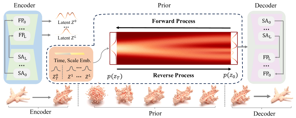
Figure 1: An overview of the proposed multi-scale latent diffusion model. Both the VAE and the latent point diffusion model use Set Abstraction modules and Feature Propagation modules. The details of the diffusion prior are shown in Figure 2.

In this section, we will introduce our hierarchical VAE framework, the multi-scale latent point diffusion prior, and the latent consistency model.

3.1 Hierarchical VAE Framework

We begin by formally introducing the latent diffusion framework, which is essentially a hierarchical VAE. We denote a point cloud as $X\in\mathbb{R}^{N\times 3}$, consisting of $N$ points with 3D coordinates. We then introduce a hierarchy of latent variables with different spatial scales/resolutions, denoting as $\mathcal{Z}=\{Z^{0},Z^{1},\dots,Z^{L}\}$, where $L$ is the number of hierarchy levels. We use superscript to denote the index of scales. Here $Z^{l}\in\mathbb{R}^{N_{l}\times C_{l}}$ where $N_{l}$ and $C_{l}$ are the number of points and the number of channels at the $l$-th level latent space respectively. Note that $C_{l}=3+D_{l}$, where $D_{l}$ represents the extra dimension. At the $0$-th, we have $N_{0}=N$ and $N_{l}>N_{l+1}$ for any $l=0,\dots,L-1$. In other words, the $Z^{0}$ is latent point representation whereas $Z^{l}$ are latent super-point (i.e., a subset of points) representations for any $l>0$. The details of latent layers and points in each level are demonstrated in Section 4 .

The backbone of our hierarchical VAE consists of an encoder $q_{\phi}(\mathcal{Z}|X)$, a decoder $p_{\psi}(X|\mathcal{Z})$, and a prior $p(\mathcal{Z})$, where $\phi$ and $\psi$ are the learnable parameters. Specifically, our encoder is designed as follows,

$$q_{\phi}(\mathcal{Z}|X):=q_{\phi}(Z^{L}|X)\prod_{l=L-1}^{0}q_{\phi}(Z^{l}|Z^{l+1},X),$$ (1)

where $q_{\phi}(Z^{L}|X)$ and $q_{\phi}(Z^{l}|Z^{l+1},X)$ are assumed to be factorized Gaussian distributions with learnable mean and fixed variance. Our decoder and prior take the simple form $p_{\psi}(X|\mathcal{Z}):=p_{\psi}(X|Z^{0})$ and $p(\mathcal{Z}):=\prod_{l=0}^{L}p(Z^{l})$ respectively. Here $p(Z^{l}):=\mathcal{N}(\bm{0},I)$. The decoder $p_{\psi}(X|Z^{0})$ is parameterized as a factorized Laplace distribution with learnable means and unit scale, corresponding to an L1 reconstruction error.

The overall architecture is illustrated in Figure 1. As shown, both the encoder and the decoder consist of multiple Set Abstraction (SA) and Feature Propagation (FP) modules. Each SA module contains point-voxel convolution (PVC) layers [26], followed by a Grouper block, which includes the sampling and grouping layers introduced by [39]. Each FP module consists of a nearest-neighbor interpolation operation, followed by MLPs and PVC layers.

First Stage Training. We train the encoder and the decoder with a fixed prior by maximizing the modified evidence lower bound (ELBO),

$$\mathcal{L}_{\text{ELBO}}(\phi,\psi) =\mathbb{E}_{p_{\text{data}}(X),q_{\phi}(\mathcal{Z}|X)}[\text{log}\>p_{\psi}(X|\mathcal{Z})$$

$$-\lambda D_{KL}(q_{\phi}(\mathcal{Z}|X)\|p(\mathcal{Z}))]$$ (2)

Here $p_{\text{data}}(X)$ represents the unknown data distribution of 3D point clouds. The hyperparameter $\lambda$ controls the trade-off between the reconstruction error and the Kullback-Leibler (KL) divergence.

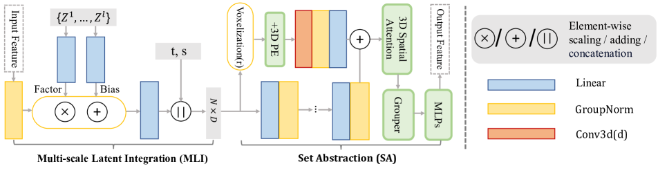
Figure 2: An illustration of the network architecture of the latent diffusion prior. We denote the voxel grid size as $r$, and the hidden dimension as $D$ and $D^{{}^{\prime}}$.

3.2 Multi-Scale Latent Point Diffusion As Prior

After learning the encoder and the decoder in the first stage, we fix them and train a denoising diffusion based prior in the latent point space. Note that we have a set of latent representations $\mathcal{Z}=\{Z^{0},\dots,Z^{L}\}$ ranging from point to super-point levels output by the hierarchical encoder. It is natural to select the latent variable with the coarsest scale (lowest spatial resolution), i.e., $Z^{L}$, to build a diffusion prior since it would enable efficient diffusion in a low-dimensional latent space. However, as demonstrated in prior work [56], point-level latent variables remain crucial for producing high-quality 3D shapes. We thus focus on the point-level latent variable $Z^{0}$ and design mechanisms to fuse multi-scale information. Specifically, we introduce a multi-scale latent point diffusion prior as below,

$$p(\mathcal{Z}):=p_{\theta}(Z^{0}|\mathcal{Z}^{\setminus{0}})\prod_{l=1}^{L}p_{\theta}(Z^{l}),$$ (3)

where $\mathcal{Z}^{\setminus{0}}=\{Z^{1},\dots,Z^{L}\}$. Here $p_{\theta}(Z^{l})$ is again a factorized standard Normal distribution, whereas $p_{\theta}(Z^{0}|\mathcal{Z}^{\setminus{0}})$ is a diffusion model. This design is crucial for enabling efficient sampling and consistency distillation, as it requires learning only one conditional prior while keeping others fixed. In contrast, previous work such as LION [56] needs to learn multiple priors corresponding to different levels in the hierarchy, which significantly complicates sampling and distillation. Similar to other diffusion models, our model consists of the forward and the reverse processes.

Forward Process. Following diffusion models [9], given initial latent point feature $Z^{0}\sim q_{\phi}(Z^{0}|X)$ output by the encoder, we gradually add noise as follows,

$$q(Z^{0}_{1:T}|Z^{0},\mathcal{Z}^{\setminus{0}}):=\prod_{t=1}^{T}q(Z^{0}_{t}|Z^{0}_{t-1}),$$ (4)

$$q(Z^{0}_{t}|Z^{0}_{t-1}):=\mathcal{N}(Z^{0}_{t};\sqrt{1-\beta_{t}}Z^{0}_{t-1},\beta_{t}I),$$ (5)

where $Z^{0}_{0}:=Z^{0}$ and we use subscripts to denote diffusion steps. $T$ represents the number of diffusion steps, $q(Z_{t}|Z^{0}_{t-1})$ is a Gaussian transition probability with variance schedule $\beta_{1},\ldots,\beta_{T}$. We adopt a linear variance schedule in the diffusion process. The choice of $\beta_{t}$ ensures that the chain approximately converges to the stationary distribution, i.e., standard Gaussian distribution $q(Z_{T}|Z^{0},\mathcal{Z}^{\setminus{0}})\approx\mathcal{N}(Z_{T};0,I)$ after $T$ steps.

Reverse Process. In the reverse process, given the intial noise $Z^{0}_{T}\sim\mathcal{N}(Z^{0}_{T};\bm{0},I)$, we learn to gradually denoise to recover the observed latent point feature $Z^{0}$ as follows,

$$p_{\theta}(Z^{0}_{0:T}|\mathcal{Z}^{\setminus{0}}) :=p(Z^{0}_{T})\prod_{t=1}^{T}p_{\theta}(Z^{0}_{t-1}|Z^{0}_{t},\mathcal{Z}^{\setminus{0}})$$ (6)

$$p_{\theta}(Z^{0}_{t-1}|Z^{0}_{t},\mathcal{Z}^{\setminus{0}}) :=\mathcal{N}(Z^{0}_{t-1};\mu_{\theta}(Z^{0}_{t},t,\mathcal{Z}^{\setminus{0}}),\sigma_{t}^{2}I),$$ (7)

where the mean function $\mu_{\theta}(\cdot,\cdot,\cdot)$ of the denoising distribution could be constructed by a neural network with learnable parameters $\theta$. In particular, following DDPM, we adopt the reparameterization $\mu_{\theta}(Z^{0}_{t},t,\mathcal{Z}^{\setminus{0}})=(Z^{0}_{t}-\beta_{t}\epsilon_{\theta}(Z^{0}_{t},t,\mathcal{Z}^{\setminus{0}})/\sqrt{1-\bar{\alpha}_{t}})/\sqrt{\alpha_{t}}$, where $\alpha_{t}:=1-\beta_{t}$ and $\bar{\alpha}_{t}:=\prod_{s=1}^{t}\alpha_{s}$. The variance $\sigma_{t}$ is a hyperparameter and set to 1. Therefore, learning our multi-scale latent point diffusion prior is essentially learning the noise-prediction function $\epsilon_{\theta}(\cdot,\cdot,\cdot)$ parameterized by $\theta$.

Second Stage Training. To train the prior, we ideally aim to minimize the KL divergence between the so-called aggregated posterior $q(\mathcal{Z})=\int p_{\text{data}}(X)q_{\phi}(\mathcal{Z}|X)\mathrm{d}X$ and the prior $p_{\theta}(\mathcal{Z})$. However, it is again intractable so that we need to resort to the negative ELBO, which can be equivalently written as the following denoising score matching type of objective,

$$\mathcal{L}_{\text{SM}}(\theta)=\mathbb{E}_{t,X,\mathcal{Z},\epsilon}\|\epsilon-\epsilon_{\theta}(Z^{0}_{t},t,\mathcal{Z}^{\setminus{0}})\|_{2}^{2},$$ (8)

where the expectation is taken with respect to $t\sim U([T])$, $X\sim p_{\text{data}}(X)$, $\mathcal{Z}\sim q_{\phi}(\mathcal{Z}|X)$, $\epsilon\sim\mathcal{N}(\bm{0},I)$. Here $U([T])$ is the uniform distribution over $\{1,2,\dots,T\}$. Following [56], we utilize the mixed score parameterization, which linearly combines the input noisy sample and the noise predicted by the network, resulting in a residual correction that links the input and output of the noise function $\epsilon_{\theta}$. More details are provided in Supplementary Materials.

3.3 Architecture Design

We now introduce the specific architecture of our noise prediction function $\epsilon_{\theta}$. Our backbone network is based on Point-Voxel CNNs (PVCNNs) [26]. To integrate multi-scale latent point feature, we propose the multi-scale latent integration (MLI) module before each SA and FP module of PVCNNs. We also adopt a 3D spatial attention mechanism in each point-voxel convolution (PVC) module, allowing the model to selectively attend to informative areas, as shown in Figure 2.

Multi-Scale Latent Integration. To better capture geometric patterns of 3D shapes, we propose the multi-scale latent integration (MLI) module to fuse latent variables across multiple scales/resolutions. As shown in Figure 2, at the diffusion step $t$, the $s$-th MLI module takes the feature map $F_{s}$ as input, where $F_{0}=Z^{0}_{t}$. Specifically, given the high-resolution feature map $F_{s}$ and the target feature $F$, we modulate the normalized target feature $F$ with the scaling parameters of both the two-dimensional scale and the high-scale features $F^{i}$, resulting in an intermediate representation as follows:

$$F_{s+1} =\left[\text{MLP}\circ\text{ReLU}(\text{Linear}(\mathcal{Z}^{\setminus{0}})\odot\text{Norm}(F_{s})\right.$$

$$+\left.\text{Linear}(\mathcal{Z}^{\setminus{0}}))~{}\|~{}\text{Pos}(t)~{}\|~{}\text{Pos}(k)\right],$$ (9)

where Norm is the layer normalization [2] and Linear denotes a linear layer. MLP consists of two linear layers. $\odot$ denotes element-wise product and $\circ$ means function composition. $[\cdot\|\cdot]$ means concatenation of vectors. Pos$(\cdot)$ is the positional embedding function. To enable scale-time awareness in the model, we further modulate the feature with positional embedding of scale and time. The feature is fed to the following SA and FP modules to predict the noise.

3D Spatial Attention Mechanism. To help latent point representations better capture 3D spatial information , we design a 3D spatial attention mechanism. Our intuition is that closer points in 3D space would have a stronger correlation, thus higher attention values. We introduce a pairwise bias term that depends on the 3D distances between points. Specifically, in PVC, following [26], we first use PointNet++[39] to extract the local features $F_{p}$ from the point cloud. We then convert the point cloud data into voxels, enabling the application of 3D convolution operations to obtain voxel features $F_{v}$. These are then fused to get the combined feature $F_{a}=\text{Add}(F_{p},\text{MLP}(F_{v}))$. For $F_{a}$, we compute the pairwise spatial distance matrix $B\in\mathbb{R}^{n^{i}\times n^{i}}$ between different point pairs at the current scale, where $n^{i}$ is the number of points at the current scale $i$, and use it as a bias in computing the attention,

$$F_{v}=\text{softmax}\left(\frac{QK^{T}}{\sqrt{d}}+B\right)\cdot V$$ (10)

where $Q$, $K$, and $V$ are query, key, and value respectively in the standard attention module. We add this module to each PVC layer across all scales to make the model’s attention conform to the 3D distances between points. Additionally, following [34], we add 3D positional embeddings to adaptively aggregate feature from voxelized point clouds. In each PVC layer, given voxelized input $V\in\mathbb{R}^{v\times v\times v\times c}$, where $c$ is the embedding dimension and $v^{3}$ denotes the number of voxelized tokens, we add sine-cosine-based 3D positional embeddings to all input tokens.

3.4 Multi-Scale Latent Point Consistency Models

Since the diffusion models are notoriously slow in sampling, we explore the consistency models (CMs) [50] in the latent diffusion framework to accelerate the generation of 3D shapes. At the core of CMs, a consistency map is introduced to map any noisy data point on the trajectory of probability-flow ordinary differential equations (PF-ODEs) to the starting point, i.e., clean data. There are two ways to train such a consistency map [50], i.e., consistency distillation and consistency training. The former requires a pretrained teacher model whereas the latter trains the consistency map from scratch. We explored both options and found consistency distillation works well, whereas consistency training is sensitive to hyperparameters.

Specifically, we first rewrite the reverse process in the continuous-time setting following [48, 28],

$$\frac{\mathrm{d}Z^{0}_{t}}{\mathrm{d}t}=\frac{\mathrm{d}\log\alpha_{t}}{\mathrm{d}t}Z^{0}_{t}+\left(\frac{\mathrm{d}\log\alpha_{t}}{2\sigma_{t}\mathrm{d}t}-\frac{\mathrm{d}\log\alpha_{t}}{\mathrm{d}t}\sigma_{t}\right)\epsilon_{\theta}(Z^{0}_{t},t,\mathcal{Z}^{\setminus{0}})$$ (11)

where $\epsilon_{\theta}(Z^{0}_{t},t,\mathcal{Z}^{\setminus{0}})$ is the noise prediction model and $\alpha_{t},\sigma_{t}$ are determined by the noise schedule as aforementioned. Samples can be drawn by solving the PF-ODE from $T$ to $0$. To achieve consistency distillation, we introduce a consistency map $f_{\hat{\theta}}:(Z^{0}_{t},t,\mathcal{Z}^{\setminus{0}})\mapsto Z_{0}^{0}$ to directly predict the solution of PF-ODE in Equation 11. For $t=0$, we parameterize $f_{\hat{\theta}}$ using the noise prediction model $\hat{\epsilon}_{\theta}$:

$$f_{\hat{\theta}}(Z^{0}_{t},t,\mathcal{Z}^{\setminus{0}})=c_{\text{skip}}(t)Z^{0}_{t}+c_{\text{out}}(t)\left(\frac{Z^{0}_{t}-\sigma_{t}\hat{\epsilon}_{\hat{\theta}}(Z^{0}_{t},t,\mathcal{Z}^{\setminus{0}})}{\alpha_{t}}\right),$$ (12)

where $c_{\text{skip}}(0)=1$, $c_{\text{out}}(0)=0$, and $\hat{\epsilon}_{\hat{\theta}}(z,c,t)$ is a noise prediction model whose initialized parameters are the same as those of the teacher diffusion model. Note that $f_{\hat{\theta}}$ can be parameterized in various ways, depending on the teacher model’s parameterization of the diffusion model.

We assume that an effective ODE solver can be used to approximate the integral on the right side of Equation 11 from any starting time to the ending time. Note that we only use the solver during training and not during sampling. We aim to predict the solution of the PF-ODE by minimizing the consistency distillation loss [50]:

$$\mathcal{L}_{\text{CD}}(\hat{\theta},\hat{\theta}^{-};\Psi)=$$

$$\mathbb{E}_{n,\mathcal{Z}^{\setminus{0}},Z^{0}_{t_{n+1}}}\left[d\left(f_{\hat{\theta}}\left(Z^{0}_{t_{n+1}},\mathcal{Z}^{\setminus{0}},t_{n+1}\right),f_{\hat{\theta}^{-}}\left(\hat{Z}^{0}_{t_{n}},\mathcal{Z}^{\setminus{0}},t_{n}\right)\right)\right],$$ (13)

where $\hat{Z}^{0}_{t_{n}}=Z^{0}_{t_{n+1}}+(t_{n}-t_{n+1})\Psi(Z^{0}_{t_{n+1}},t_{n+1},t_{n},\mathcal{Z}^{\setminus{0}})$ is the solution of the PF-ODE obtained via calling the ODE solver $\Psi$ from time $t_{n+1}$ to $t_{n}$. $d(\bm{x},\bm{y})=\|\bm{x}-\bm{y}\|^{2}_{2}$.

4 Experiments

In this section, we train the multi-scale latent diffusion model on the Shapenet dataset and obtain MLPCM using the latent consistent distillation. We first introduce the dataset and evaluation metrics. Then we evaluate the performance of MLPCM on the Single-class 3D point cloud generation task. Next, we compare the results of MLPCM with a large number of baselines on multi-class unconditional 3D shape generation in terms of the performance, sampling time, and model parameters. Finally, we give a detailed ablation study on the effectiveness of invidual contributions.

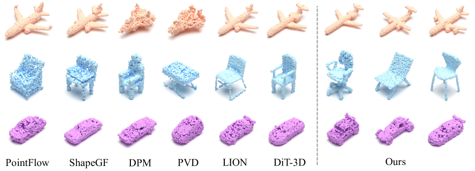
Figure 3: Unconditional shape generation with 2,048 points for the classes airplane, car, and chair using class-specific models, trained on the ShapeNet dataset from PointFlow with global normalization.

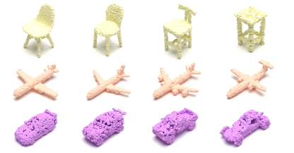
Figure 4: Qualitative visualizations of high-fidelity and diverse 3D point cloud generation.

4.1 Datasets & Metrics

Datasets. To compare MLPCM against existing methods, we use ShapeNet [4], the most widely used dataset to benchmark 3D shape generative models. Following previous works [56, 55, 61, 30], we train on three categories: airplane, chair, car and primarily rely on PointFlow’s [55] dataset splits and preprocssing, which normalizes the data globally across the whole dataset. However, some baselines require per-shape normalization [19, 58, 3, 10]; hence, we also train on such data. In addition, following [56], we also perform the task of multi-class unconditional 3D shape generation on the ShapeNet-Vol [38, 37] dataset, where the data is normalized per-shape.

Evaluation. Following recent works [55, 61, 56], we use 1-NNA, with both Chamfer distance (CD) and earth mover distance (EMD), as our main metric. It quantifies the similarity between the distribution of generated shapes and that of shapes from the validation set and measures both quality and diversity [55].

4.2 Single-Class 3D Point Cloud Generation

Implementation Our implementation is based on the PyTorch [36]. The input point cloud size is $2048\times 3$. Both our VAE encoder and decoder are built upon PVCNN [26], consisting of 4 layers of SA modules and FP modules. The voxel grid sizes of PVC at different scales are $32$, $16$, $8$, and $8$, respectively. We adopt the Farthest Point Sampling (FPS) algorithm for sampling in the Grouper block, with the sampled center points being $1024$, $256$, $64$, and $16$. KNN (K-Nearest Neighbors) is used to aggregate local neighborhood features, with $32$ neighbors for each point in the Grouper. We apply a dropout rate of $0.1$ to all dropout layers in the VAE. Following [56], we initialize our VAE model so that it acts as an identity mapping between the input, latent space, and reconstruction points at the start of training. We achieve this by reducing the variance of the encoder and correspondingly weighting the skip connections. Our latent prior also consists of 4 layers of SA modules and FP modules. The time embedding and multi-scale latent representations are concatenated with the point features at the input of each corresponding SA and FP layer. We adopt the hybrid denoising score network parameterization following [56].

Results We use the Adam optimizer [17] to train our model, where the VAE is trained for $8,000$ epochs and the diffusion prior for $24,000$ epochs, with a batch size of $128$. We set $T=1,000$ as the time steps of the diffusion process. For latent consistency distillation, we train MLPCM for $100$K iterations with a batch size of $128$, a learning rate of $2\times 10^{-4}$, and an EMA rate $\mu=0.99995$. We validate our model’s results under two settings: normalizing data across the entire dataset and normalizing each shape individually. Samples from MLPCM are shown in Figure 3 and Figure  4, and quantitative results are provided in Table 1 and Table 2. Note that TM stands for Teacher Model and LCM stands for Latent Consistency Models. MLPCM outperforms all baselines and achieves state-of-the-art performance across all categories and dataset versions. Compared to key baselines like DPM, PVD, and LION, our samples are diverse and have a better visual quality.

Table 1: Generation metrics (1-NNA↓) on airplane, chair, car categories from ShapeNet dataset from PointFlow [55]. Training and test data normalized globally into [-1, 1]. TM stands for Teacher Model and LCM stands for Latent Consistency Models.

	Airplane		Chair		Car
Method	CD	EMD	CD	EMD	CD	EMD
r-GAN [1]	98.40	96.79	83.69	99.70	94.46	99.01
l-GAN(CD) [1]	87.30	93.95	68.58	83.84	66.49	88.78
l-GAN(EMD) [1]	89.49	76.91	71.90	64.65	71.16	66.19
PointFlow [55]	75.68	70.74	62.84	60.57	58.10	56.25
SoftFlow [13]	76.05	65.80	59.21	60.05	64.77	60.09
SetVAE [14]	76.54	67.65	58.84	60.57	59.94	59.94
DPF-Net [18]	75.18	65.55	62.00	58.53	62.35	54.48
DPM [30]	76.42	86.91	60.05	74.77	68.89	79.97
PVD [61]	73.82	64.81	56.26	53.32	54.55	53.83
LION [56]	67.41	61.23	53.70	52.34	53.41	51.14
MeshDiffusion [27]	66.44	76.26	53.69	57.63	81.43	87.84
DiT-3D [34]	69.42	65.08	55.59	54.91	53.87	53.02
Ours (TM)	65.12	58.70	51.48	50.06	51.17	48.92
Ours (LCM)	67.22	60.32	53.63	51.74	53.82	52.75

Table 2: Generation results (1-NNA↓) on ShapeNet dataset from PointFlow [55]. All data normalized individually into [-1, 1].

	Airplane		Chair		Car
Method	CD	EMD	CD	EMD	CD	EMD
Tree-GAN [23]	97.53	99.88	88.37	96.37	89.77	94.89
ShapeGF [3]	81.23	80.86	58.01	61.25	61.79	57.24
SP-GAN [19]	94.69	93.95	72.58	83.69	87.36	85.94
PDGN [10]	94.94	91.73	71.83	79.00	89.35	87.22
GCA [58]	88.15	85.93	64.27	64.50	70.45	64.20
LION [56]	76.30	67.04	56.50	53.85	59.52	49.29
Ours (TM)	73.28	63.08	56.20	53.16	58.31	47.74
Ours (LCM)	75.56	66.85	58.58	55.32	61.28	49.91

4.3 Multi-Class 3D Shape Generation

Following [56], we also jointly trained the multi-scale latent diffusion model and the MLPCM model across 13 different categories (airplane, chair, car, lamp, table, sofa, cabinet, bench, phone, watercraft, speaker, display, ship, rifle). Due to the highly complex and multi-modal data distribution, jointly training a model is challenging.

We validated the model’s generation performance on the Shapenet-Vol dataset, where each shape is normalized, meaning the point coordinates are bounded within $[-1,1]$. We report the quantitative results in Table 3, comparing our method with various strong baselines under the same setting. We found that the proposed multi-scale latent diffusion model significantly outperforms all baselines, and MLPCM greatly improves sampling efficiency while maintaining performance.

Table 3: Results of joint training on 13 classes of ShapeNet-vol.

Method	CD(1- NNA↓)	EMD(1- NNA↓)
Tree-GAN [23]	96.80	96.60
PointFlow [55]	63.25	66.05
ShapeGF [3]	55.65	59.00
SetVAE [14]	79.25	95.25
PDGN [10]	71.05	86.00
DPF-Net [18]	67.10	64.75
DPM [30]	62.30	86.50
PVD [61]	58.65	57.85
LION [56]	51.85	48.95
Ours (TM)	50.17	47.84
Ours (LCM)	53.85	52.45

4.4 Sampling Time

The proposed multi-scale latent diffusion model synthesizes shapes using 1000 steps of DDPM, while MLPCM synthesizes them using only 1-4 steps, generating high-quality shapes in under 0.5 seconds. This makes real-time interactive applications feasible. In Table 4, we compare the sampling time and quality of generating a point cloud sample (2048 points) from noise using different DDPM, DDIM [46] sampling methods, and MLPCM. When using $\leq 10$ steps, DDIM’s performance degrades significantly, whereas MLPCM can produce visually high-quality shapes in just a few steps or even one step.

Table 4: The sampling rates and generation quality of our model with various methods. Our approach achieves high-quality shape generation within 0.5 seconds while maintaining quality.

Method	steps	time(sec)	CD(1- NNA↓)	EMD(1- NNA↓)
LION(DDPM) [56]	1000	27.09	53.41	51.14
LION(DDIM) [56]	1000	27.09	54.85	53.26
LION(DDIM) [56]	100	3.07	56.04	54.97
LION(DDIM) [56]	10	0.47	90.38	95.4
Ours(TM)	1000	25.16	51.17	48.92
Ours(LCM)	1	0.18	79.46	82.00
Ours(LCM)	4	0.31	53.82	52.75

4.5 Ablation Study

In this section, we conduct the ablation study to investigate the effectiveness of the individual design components introduced in the multi-scale latent diffusion model, including the multi-scale latents, 3D Spatial Attention Mechanism, and the additional dimensions of the latent points.

Ablation on the Key Design Components. We perform the ablation study on the Car category. For the configuration without multi-scale latent representations, we consider two scenarios: one using only point-level latent features to capture fine-grained details and another using only shape-level features to focus on global structure. This allows us to assess the impact of each representation scale individually. The model sizes are kept nearly identical across all settings to ensure fair comparison. As shown in Table 5, the full model, integrating multi-scale latent representations and the 3D spatial attention mechanism, consistently outperforms the simplified settings across all evaluation metrics. This demonstrates the effectiveness of combining fine-grained local information with global shape context, along with the attention mechanism, in achieving more accurate and coherent reconstructions.

Table 5: Ablation studies on key 3D design components on the car category. PL and SL represent the point-level latents and shape-level latents, respectively, and 3DSA represents the 3D Spatial Attention Mechanism.

PL	SL	3DSA	CD(1- NNA$\downarrow$)	EMD(1- NNA$\downarrow$)
	$\checkmark$	$\checkmark$	74.29	72.81
$\checkmark$		$\checkmark$	53.40	51.96
$\checkmark$	$\checkmark$		53.02	50.75
$\checkmark$	$\checkmark$	$\checkmark$	51.17	48.92

Table 6: Ablation on the number of extra dimension $D_{l}$ of the latent points, on the car category.

Extra Latent Dim	CD(1- NNA↓)	EMD(1- NNA↓)
0	54.56	52.79
1	51.17	48.92
3	56.88	55.27
5	59.06	51.90

Ablation on Extra Dimension for Latent Points. We ablate the additional latent point dimension $D_{l}$ on the Car category in Table 6. We experimented with several different additional dimensions for the latent points, ranging from 0 to 5, where $D_{l}=1$ provided the best overall performance. As the additional dimensions increase, we observe a decrease in the 1-NNA score. We thus use $D_{l}=1$ for all other experiments.

5 Conclusion

In this paper, we propose the Multi-Scale Latent Point Consistency Model (MLPCM) to address the task of efficient point-cloud-based 3D shape generation. We first construct a multi-scale latent diffusion model, which includes a point encoder based on multi-scale voxel convolutions, a multi-scale denoising diffusion prior with 3D spatial attention, and a voxel-convolution-based decoder. The diffusion prior model, which integrates multi-scale information, effectively captures both local and global geometric features of 3D objects, while the 3D spatial attention mechanism helps the model better capture spatial information and feature correlations. Moreover, MLPCM leverages consistency distillation to compress the prior into a one-step generator. On the widely used ShapeNet and ShapeNet-Vol datasets, the proposed multi-scale latent diffusion model achieves state-of-the-art performance, and MLPCM achieves a 100x speedup during sampling while surpassing the state-of-the-art diffusion models in terms of shape quality and diversity. In the future, we are interested in extending MLPCM to other diverse 3D representations such as meshes.

References

- Achlioptas et al. [2018] Panos Achlioptas, Olga Diamanti, Ioannis Mitliagkas, and Leonidas Guibas. Learning representations and generative models for 3d point clouds. In International conference on machine learning, pages 40–49. PMLR, 2018.
- Ba [2016] Jimmy Lei Ba. Layer normalization. arXiv preprint arXiv:1607.06450, 2016.
- Cai et al. [2020] Ruojin Cai, Guandao Yang, Hadar Averbuch-Elor, Zekun Hao, Serge Belongie, Noah Snavely, and Bharath Hariharan. Learning gradient fields for shape generation. In Computer Vision–ECCV 2020: 16th European Conference, Glasgow, UK, August 23–28, 2020, Proceedings, Part III 16, pages 364–381. Springer, 2020.
- Chang et al. [2015] Angel X Chang, Thomas Funkhouser, Leonidas Guibas, Pat Hanrahan, Qixing Huang, Zimo Li, Silvio Savarese, Manolis Savva, Shuran Song, Hao Su, et al. Shapenet: An information-rich 3d model repository. arXiv preprint arXiv:1512.03012, 2015.
- Cheng et al. [2023] Yen-Chi Cheng, Hsin-Ying Lee, Sergey Tulyakov, Alexander G Schwing, and Liang-Yan Gui. Sdfusion: Multimodal 3d shape completion, reconstruction, and generation. In Proceedings of the IEEE/CVF Conference on Computer Vision and Pattern Recognition, pages 4456–4465, 2023.
- Gal et al. [2021] Rinon Gal, Amit Bermano, Hao Zhang, and Daniel Cohen-Or. Mrgan: Multi-rooted 3d shape representation learning with unsupervised part disentanglement. In Proceedings of the IEEE/CVF International Conference on Computer Vision, pages 2039–2048, 2021.
- Goodfellow et al. [2020] Ian Goodfellow, Jean Pouget-Abadie, Mehdi Mirza, Bing Xu, David Warde-Farley, Sherjil Ozair, Aaron Courville, and Yoshua Bengio. Generative adversarial networks. Communications of the ACM, 63(11):139–144, 2020.
- Hao et al. [2021] Zekun Hao, Arun Mallya, Serge Belongie, and Ming-Yu Liu. Gancraft: Unsupervised 3d neural rendering of minecraft worlds. In Proceedings of the IEEE/CVF International Conference on Computer Vision, pages 14072–14082, 2021.
- Ho et al. [2020] Jonathan Ho, Ajay Jain, and Pieter Abbeel. Denoising diffusion probabilistic models. Advances in neural information processing systems, 33:6840–6851, 2020.
- Hui et al. [2020] Le Hui, Rui Xu, Jin Xie, Jianjun Qian, and Jian Yang. Progressive point cloud deconvolution generation network. In Computer Vision–ECCV 2020: 16th European Conference, Glasgow, UK, August 23–28, 2020, Proceedings, Part XV 16, pages 397–413. Springer, 2020.
- Jolicoeur-Martineau et al. [2021] Alexia Jolicoeur-Martineau, Ke Li, Rémi Piché-Taillefer, Tal Kachman, and Ioannis Mitliagkas. Gotta go fast when generating data with score-based models. arXiv preprint arXiv:2105.14080, 2021.
- Karras et al. [2019] Tero Karras, Samuli Laine, and Timo Aila. A style-based generator architecture for generative adversarial networks. In Proceedings of the IEEE/CVF conference on computer vision and pattern recognition, pages 4401–4410, 2019.
- Kim et al. [2020] Hyeongju Kim, Hyeonseung Lee, Woo Hyun Kang, Joun Yeop Lee, and Nam Soo Kim. Softflow: Probabilistic framework for normalizing flow on manifolds. Advances in Neural Information Processing Systems, 33:16388–16397, 2020.
- Kim et al. [2021] Jinwoo Kim, Jaehoon Yoo, Juho Lee, and Seunghoon Hong. Setvae: Learning hierarchical composition for generative modeling of set-structured data. In Proceedings of the IEEE/CVF Conference on Computer Vision and Pattern Recognition, pages 15059–15068, 2021.
- Kimura et al. [2021] Takumi Kimura, Takashi Matsubara, and Kuniaki Uehara. Chartpointflow for topology-aware 3d point cloud generation. In Proceedings of the 29th ACM International Conference on Multimedia, pages 1396–1404, 2021.
- Kingma [2013] Diederik P Kingma. Auto-encoding variational bayes. arXiv preprint arXiv:1312.6114, 2013.
- Kingma [2014] Diederik P Kingma. Adam: A method for stochastic optimization. arXiv preprint arXiv:1412.6980, 2014.
- Klokov et al. [2020] Roman Klokov, Edmond Boyer, and Jakob Verbeek. Discrete point flow networks for efficient point cloud generation. In European Conference on Computer Vision, pages 694–710. Springer, 2020.
- Li et al. [2021] Ruihui Li, Xianzhi Li, Ka-Hei Hui, and Chi-Wing Fu. Sp-gan: Sphere-guided 3d shape generation and manipulation. ACM Transactions on Graphics (TOG), 40(4):1–12, 2021.
- Li et al. [2022] Shidi Li, Miaomiao Liu, and Christian Walder. Editvae: Unsupervised parts-aware controllable 3d point cloud shape generation. In Proceedings of the AAAI Conference on Artificial Intelligence, pages 1386–1394, 2022.
- Li et al. [2023] Yuhan Li, Yishun Dou, Xuanhong Chen, Bingbing Ni, Yilin Sun, Yutian Liu, and Fuzhen Wang. Generalized deep 3d shape prior via part-discretized diffusion process. In Proceedings of the IEEE/CVF Conference on Computer Vision and Pattern Recognition, pages 16784–16794, 2023.
- Litany et al. [2018] Or Litany, Alex Bronstein, Michael Bronstein, and Ameesh Makadia. Deformable shape completion with graph convolutional autoencoders. In Proceedings of the IEEE conference on computer vision and pattern recognition, pages 1886–1895, 2018.
- Liu et al. [2018] Xinyue Liu, Xiangnan Kong, Lei Liu, and Kuorong Chiang. Treegan: syntax-aware sequence generation with generative adversarial networks. In 2018 IEEE International Conference on Data Mining (ICDM), pages 1140–1145. IEEE, 2018.
- Liu et al. [2022] Xingchao Liu, Chengyue Gong, and Qiang Liu. Flow straight and fast: Learning to generate and transfer data with rectified flow. arXiv preprint arXiv:2209.03003, 2022.
- Liu et al. [2023a] Xingchao Liu, Xiwen Zhang, Jianzhu Ma, Jian Peng, et al. Instaflow: One step is enough for high-quality diffusion-based text-to-image generation. In The Twelfth International Conference on Learning Representations, 2023a.
- Liu et al. [2019] Zhijian Liu, Haotian Tang, Yujun Lin, and Song Han. Point-voxel cnn for efficient 3d deep learning. Advances in neural information processing systems, 32, 2019.
- Liu et al. [2023b] Zhen Liu, Yao Feng, Michael J Black, Derek Nowrouzezahrai, Liam Paull, and Weiyang Liu. Meshdiffusion: Score-based generative 3d mesh modeling. arXiv preprint arXiv:2303.08133, 2023b.
- Lu et al. [2022a] Cheng Lu, Yuhao Zhou, Fan Bao, Jianfei Chen, Chongxuan Li, and Jun Zhu. Dpm-solver: A fast ode solver for diffusion probabilistic model sampling in around 10 steps. Advances in Neural Information Processing Systems, 35:5775–5787, 2022a.
- Lu et al. [2022b] Cheng Lu, Yuhao Zhou, Fan Bao, Jianfei Chen, Chongxuan Li, and Jun Zhu. Dpm-solver++: Fast solver for guided sampling of diffusion probabilistic models. arXiv preprint arXiv:2211.01095, 2022b.
- Luo and Hu [2021] Shitong Luo and Wei Hu. Diffusion probabilistic models for 3d point cloud generation. In Proceedings of the IEEE/CVF conference on computer vision and pattern recognition, pages 2837–2845, 2021.
- Lyu et al. [2022] Zhaoyang Lyu, Xudong Xu, Ceyuan Yang, Dahua Lin, and Bo Dai. Accelerating diffusion models via early stop of the diffusion process. arXiv preprint arXiv:2205.12524, 2022.
- Meng et al. [2023] Chenlin Meng, Robin Rombach, Ruiqi Gao, Diederik Kingma, Stefano Ermon, Jonathan Ho, and Tim Salimans. On distillation of guided diffusion models. In Proceedings of the IEEE/CVF Conference on Computer Vision and Pattern Recognition, pages 14297–14306, 2023.
- Mittal et al. [2022] Paritosh Mittal, Yen-Chi Cheng, Maneesh Singh, and Shubham Tulsiani. Autosdf: Shape priors for 3d completion, reconstruction and generation. In Proceedings of the IEEE/CVF Conference on Computer Vision and Pattern Recognition, pages 306–315, 2022.
- Mo et al. [2023] Shentong Mo, Enze Xie, Ruihang Chu, Lanqing Hong, Matthias Niessner, and Zhenguo Li. Dit-3d: Exploring plain diffusion transformers for 3d shape generation. Advances in neural information processing systems, 36:67960–67971, 2023.
- Nichol et al. [2021] Alex Nichol, Prafulla Dhariwal, Aditya Ramesh, Pranav Shyam, Pamela Mishkin, Bob McGrew, Ilya Sutskever, and Mark Chen. Glide: Towards photorealistic image generation and editing with text-guided diffusion models. arXiv preprint arXiv:2112.10741, 2021.
- Paszke et al. [2019] Adam Paszke, Sam Gross, Francisco Massa, Adam Lerer, James Bradbury, Gregory Chanan, Trevor Killeen, Zeming Lin, Natalia Gimelshein, Luca Antiga, et al. Pytorch: An imperative style, high-performance deep learning library. Advances in neural information processing systems, 32, 2019.
- Peng et al. [2020] Songyou Peng, Michael Niemeyer, Lars Mescheder, Marc Pollefeys, and Andreas Geiger. Convolutional occupancy networks. In Computer Vision–ECCV 2020: 16th European Conference, Glasgow, UK, August 23–28, 2020, Proceedings, Part III 16, pages 523–540. Springer, 2020.
- Peng et al. [2021] Songyou Peng, Chiyu Jiang, Yiyi Liao, Michael Niemeyer, Marc Pollefeys, and Andreas Geiger. Shape as points: A differentiable poisson solver. Advances in Neural Information Processing Systems, 34:13032–13044, 2021.
- Qi et al. [2017] Charles Ruizhongtai Qi, Li Yi, Hao Su, and Leonidas J Guibas. Pointnet++: Deep hierarchical feature learning on point sets in a metric space. Advances in neural information processing systems, 30, 2017.
- Ramesh et al. [2022] Aditya Ramesh, Prafulla Dhariwal, Alex Nichol, Casey Chu, and Mark Chen. Hierarchical text-conditional image generation with clip latents. arXiv preprint arXiv:2204.06125, 1(2):3, 2022.
- Ren et al. [2024] Xuanchi Ren, Jiahui Huang, Xiaohui Zeng, Ken Museth, Sanja Fidler, and Francis Williams. Xcube: Large-scale 3d generative modeling using sparse voxel hierarchies. In Proceedings of the IEEE/CVF Conference on Computer Vision and Pattern Recognition, pages 4209–4219, 2024.
- Rombach et al. [2022] Robin Rombach, Andreas Blattmann, Dominik Lorenz, Patrick Esser, and Björn Ommer. High-resolution image synthesis with latent diffusion models. In Proceedings of the IEEE/CVF conference on computer vision and pattern recognition, pages 10684–10695, 2022.
- Salimans and Ho [2022] Tim Salimans and Jonathan Ho. Progressive distillation for fast sampling of diffusion models. arXiv preprint arXiv:2202.00512, 2022.
- Shu et al. [2019] Dong Wook Shu, Sung Woo Park, and Junseok Kwon. 3d point cloud generative adversarial network based on tree structured graph convolutions. In Proceedings of the IEEE/CVF international conference on computer vision, pages 3859–3868, 2019.
- Sohn et al. [2015] Kihyuk Sohn, Honglak Lee, and Xinchen Yan. Learning structured output representation using deep conditional generative models. Advances in neural information processing systems, 28, 2015.
- Song et al. [2020a] Jiaming Song, Chenlin Meng, and Stefano Ermon. Denoising diffusion implicit models. arXiv preprint arXiv:2010.02502, 2020a.
- Song and Ermon [2019] Yang Song and Stefano Ermon. Generative modeling by estimating gradients of the data distribution. Advances in neural information processing systems, 32, 2019.
- Song et al. [2020b] Yang Song, Jascha Sohl-Dickstein, Diederik P Kingma, Abhishek Kumar, Stefano Ermon, and Ben Poole. Score-based generative modeling through stochastic differential equations. arXiv preprint arXiv:2011.13456, 2020b.
- Song et al. [2021] Yang Song, Conor Durkan, Iain Murray, and Stefano Ermon. Maximum likelihood training of score-based diffusion models. Advances in neural information processing systems, 34:1415–1428, 2021.
- Song et al. [2023] Yang Song, Prafulla Dhariwal, Mark Chen, and Ilya Sutskever. Consistency models. arXiv preprint arXiv:2303.01469, 2023.
- Tan et al. [2018] Qingyang Tan, Lin Gao, Yu-Kun Lai, and Shihong Xia. Variational autoencoders for deforming 3d mesh models. In Proceedings of the IEEE conference on computer vision and pattern recognition, pages 5841–5850, 2018.
- Valsesia et al. [2018] Diego Valsesia, Giulia Fracastoro, and Enrico Magli. Learning localized generative models for 3d point clouds via graph convolution. In International conference on learning representations, 2018.
- Watson et al. [2021] Daniel Watson, Jonathan Ho, Mohammad Norouzi, and William Chan. Learning to efficiently sample from diffusion probabilistic models. arXiv preprint arXiv:2106.03802, 2021.
- Wu et al. [2016] Jiajun Wu, Chengkai Zhang, Tianfan Xue, Bill Freeman, and Josh Tenenbaum. Learning a probabilistic latent space of object shapes via 3d generative-adversarial modeling. Advances in neural information processing systems, 29, 2016.
- Yang et al. [2019] Guandao Yang, Xun Huang, Zekun Hao, Ming-Yu Liu, Serge Belongie, and Bharath Hariharan. Pointflow: 3d point cloud generation with continuous normalizing flows. In Proceedings of the IEEE/CVF international conference on computer vision, pages 4541–4550, 2019.
- Zeng et al. [2022] Xiaohui Zeng, Arash Vahdat, Francis Williams, Zan Gojcic, Or Litany, Sanja Fidler, Karsten Kreis, et al. Lion: Latent point diffusion models for 3d shape generation. Advances in Neural Information Processing Systems, 35:10021–10039, 2022.
- Zhang et al. [2022] Biao Zhang, Matthias Nießner, and Peter Wonka. 3dilg: Irregular latent grids for 3d generative modeling. Advances in Neural Information Processing Systems, 35:21871–21885, 2022.
- Zhang et al. [2021] Dongsu Zhang, Changwoon Choi, Jeonghwan Kim, and Young Min Kim. Learning to generate 3d shapes with generative cellular automata. arXiv preprint arXiv:2103.04130, 2021.
- Zheng et al. [2022] Huangjie Zheng, Pengcheng He, Weizhu Chen, and Mingyuan Zhou. Truncated diffusion probabilistic models. arXiv preprint arXiv:2202.09671, 1(3.1):2, 2022.
- Zheng et al. [2023] Hongkai Zheng, Weili Nie, Arash Vahdat, Kamyar Azizzadenesheli, and Anima Anandkumar. Fast sampling of diffusion models via operator learning. In International conference on machine learning, pages 42390–42402. PMLR, 2023.
- Zhou et al. [2021] Linqi Zhou, Yilun Du, and Jiajun Wu. 3d shape generation and completion through point-voxel diffusion. In Proceedings of the IEEE/CVF international conference on computer vision, pages 5826–5835, 2021.