Orbital magnetic susceptibility of type-I, II, and III massless Dirac fermions in two dimensions

Abstract

We study the orbital magnetic susceptibility of tilted massless Dirac fermions in two dimensions. It is well-known that the type-I massless Dirac fermions exhibit divergingly-large diamagnetic susceptibility, whereas less is known about the types II and III cases. We first clarify that the orbital magnetic susceptibility is vanishing for the types II and III in the continuum model. We then compare the three types of Dirac fermions for the lattice models. We employ three tight-binding models with different numbers of Dirac points, all of which are two-band models defined on a square lattice. For all three models, we find that the type-I Dirac fermions show the divergingly-large orbital diamagnetic susceptibility, whereas the type-II Dirac fermions exhibit non-diverging paramagnetic susceptibility. The type-III Dirac fermions exhibit diamagnetism but its susceptibility is small compared with the type-I case.

I Introduction

The magnetic-field response of electrons in solids has been a fundamental and important issue. Under the periodic potentials of solids, the electronic states are described by the Bloch bands, and their characteristic dispersion relations as well as the wavefunctions are known to have a significant effect on the magnetic field response. In non-magnetic materials with weak spin-orbit coupling, the magnetic susceptibility consists of two contributions, i.e., the spin and the orbital magnetic susceptibilities. It has been revealed that the former is mainly governed by the density of state (DOS) around the Fermi energy, whereas the latter has rich physical pictures, namely, the interband effect plays an essential role [1, 2, 3, 4] and some of such contributions can be attributed to the topology and geometry of the Bloch wavefunctions [5, 6, 7, 8, 9, 10, 11, 12, 13].

Dirac fermions are known to be a fertile ground of studying orbital magnetic susceptibility [14, 15, 16, 17, 18, 19, 20, 21, 22, 23, 24, 25, 26]. Among various systems, the type-I massless Dirac fermions in two dimensions, which have linear dispersion and the ellipsoidal equi-energy surface around the band contact point, are known to exhibit characteristic orbital magnetic susceptibility [16, 17, 18, 27, 28, 6, 29]. To be more specific, when the chemical potential is right at the Dirac point, the orbital magnetic susceptibility is diamagnetic and diverging. Such a characteristic behavior has recently been observed experimentally in graphene [30]. Meanwhile, little has been revealed for the overtitled and critically tilted Dirac fermions, which are dubbed the type-II (overtilted) [31, 32, 33, 34, 35] and type-III (critically tilted) [36, 37, 38, 39, 40, 41, 42, 43, 44] Dirac fermions. For these two types, the DOS is not vanishing even when the chemical potential is at the Dirac point, which is in sharp contrast to the type-I Dirac fermions.

Several previous works have studied the orbital magnetic susceptibility of the tilted Dirac fermions by using the continuum model [27, 45, 46]. It has been discussed that the orbital magnetic susceptibility positively diverges in the type-II Dirac fermions, i.e., the opposite way compared with the type-I . In the present paper, we first study the continuum model where the Fermi surface forms straight lines in the type-II and type-III. We will show that the orbital magnetic susceptibility vanishes for these cases.

However, the continuum model has infinitely large Fermi surface and thus there will be some subtleties in the calculation for the real materials, such as the warping of the Fermi surfaces and/or bending at the boundary of the Brillouin zone. One can avoid these subtleties by using lattice models, since the momentum-space summation is performed within the Brillouin zone, and hence one can compare the results of all three types of the Dirac fermions in the common lattice models [48]. Therefore, in the present paper, we also study the orbital magnetic susceptibility in the lattice models to compare the three types of Dirac fermions by varying the parameters. We employ three tight-binding models with different numbers of Dirac points, all of which are two-band models defined on a square lattice. For all three models, we find that the type-I Dirac fermions show the divergingly-large diamagnetic susceptibility, whereas the type-II Dirac fermions exhibit non-diverging paramagnetic susceptibility. The type-III Dirac fermions exhibit diamagnetism but its susceptibility is small compared with the type-I case.

The rest of this paper is structured as follows. In Sec. II, we explain our model and the formulation. To be specific, we introduce the Dirac-type Hamiltonian with tilting in two dimensions and show the theoretical formula for calculating the orbital magnetic susceptibility. In addition, before arguing the lattice model, we show the results for the continuum model for the tilted Dirac fermions in Sec. II.2, where we clarify that the type-II and type-III Dirac fermions exhibit vanishing orbital magnetic susceptibility. In Sec. III, we introduce the square-lattice models. We present three Hamiltonians hosting different number of the tilted Dirac cones. We also address the characteristic band structures of the three models, namely, the Dirac cones and the van Hove singularity. Our main results are presented in Sec. IV. We numerically calculate the orbital magnetic susceptibility and discuss its chemical potential dependence as well as the temperature dependence. Section V is devoted to the detailed discussion on the results in Sec. IV. To be concrete, we discuss the role of the Dirac point for the type-II case. We also reveal that the paramagnetic peaks appearing away from the Dirac point can be explained by the intraband contribution. Finally, we present the summary of this paper in Sec. VI.

II Orbital magnetic susceptibility and the continuum model with tilting 

II.1 Orbital magnetic susceptibility

In general, orbital magnetic susceptibility is given by [3]

$$\chi=\frac{e^{2}}{2\hbar^{2}}\frac{k_{\rm B}T}{V}\sum_{n,\bm{k}}\mathrm{Tr}\left[v^{x}_{\bm{k}}{\mathcal{G}}v^{y}_{\bm{k}}{\mathcal{G}}v^{x}_{\bm{k}}{\mathcal{G}}v^{y}_{\bm{k}}{\mathcal{G}}\right],$$ (1)

where the summation is over the fermion Matsubara frequency, $\varepsilon_{n}=(2n+1)\pi k_{\rm B}T$ and the wave number $\bm{k}$. Note that we neglect the spin degrees of freedom for simplicity. In other words, the results shown in this paper is the orbital magnetic susceptibility per spin degrees of freedom. $V$ is the volume of the system (or the area for two dimensions). Tr is to take the trace over the Bloch bands and $\mathcal{G}$ is the abbreviation of the matrix form of thermal Green’s function ${\mathcal{G}}(\bm{k},i\varepsilon_{n})$ in the Bloch representation. The velocity $v^{i}_{\bm{k}}$ ($i=x,y$) is defined in the matrix form as $v^{i}_{\bm{k}}=\frac{\partial\mathcal{H}_{\bm{k}}}{\partial k_{i}}$, $e$ is the elementary charge, $\hbar$ is the reduced Planck constant, and $k_{\rm B}$ is the Boltzmann constant.

In the following, we consider two-band models whose Bloch Hamiltonians are generically given as

$$\mathcal{H}_{\bm{k}}=h_{\bm{k}}^{0}+\bm{h}_{\bm{k}}\cdot\bm{\sigma},$$ (2)

where $\bm{h}_{\bm{k}}=(h^{x}_{\bm{k}},h^{y}_{\bm{k}},h^{z}_{\bm{k}})$, and $\bm{\sigma}=(\sigma_{x},\sigma_{y},\sigma_{z})$ are the Pauli matrices. The dispersion relation of this Hamiltonian is given by $\varepsilon_{\bm{k},\pm}=h^{0}_{\bm{k}}\pm|\bm{h}_{\bm{k}}|$. Then the band touching occurs at which $|\bm{h}_{\bm{k}}|=0$ is satisfied. $h_{\bm{k}}^{0}$ gives tilting.

In this Hamiltonian, we obtain thermal Green’s function as

$${\mathcal{G}}(\bm{k},i\varepsilon_{n})=\frac{i\tilde{\varepsilon}_{n}+{\bm{h}}_{\bm{k}}\cdot\bm{\sigma}}{D},$$ (3)

with $i\tilde{\varepsilon}_{n}:=i\varepsilon_{n}-h_{\bm{k}}^{0}+\mu$ ($\mu$ is the chemical potential) and $D=(i\tilde{\varepsilon}_{n})^{2}-|\bm{h}_{\bm{k}}|^{2}$. The velocities $v^{i}_{\bm{k}}$ ($i=x,y$) are given by

$$v^{i}_{\bm{k}}=\frac{\partial h_{\bm{k}}^{0}}{\partial k_{i}}+\frac{\partial{\bm{h}}_{\bm{k}}}{\partial k_{i}}\cdot\bm{\sigma}.$$ (4)

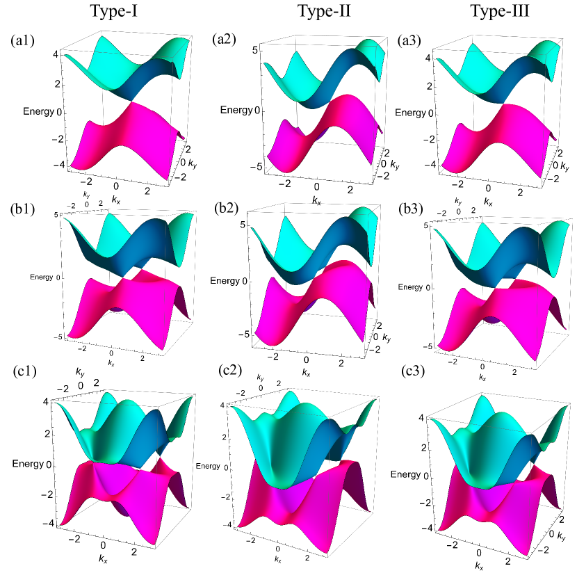
Figure 1: The band structures of the models (i) for the panels labeled by (a), (ii) for the panels labeled by (b), and (iii) for the panels labeled by (c). The panels labeled by 1, 2, and 3, are for the types I, II, and III Dirac fermions, respectively. The parameters are described in Table 1.

II.2 Continuum model of massless Dirac Hamiltonian with tilting 

Before discussing the lattice model, we consider a single massless Dirac Hamiltonian in two-dimension with tilting. In this case, we use

$$\bm{h}_{\bm{k}} =(v_{\rm F}\hbar k_{x},v_{\rm F}\hbar k_{y},0),$$ (5)

$$h_{\bm{k}}^{0} =-\alpha v_{\rm F}\hbar k_{x},$$ (6)

where $v_{\rm F}$ is the Fermi velocity and the parameter $\alpha$ represents the degree of tilting in the $k_{x}$-direction. The dispersion relation is given by $\varepsilon_{\bm{k},\pm}=-\alpha v_{\rm F}\hbar k_{x}\pm v_{\rm F}\hbar k$ with $k=|\bm{k}|$. The type I (II) corresponds to $0\leq\alpha<1$ ($\alpha>1$) and The type III corresponds to $\alpha=1$ where the Dirac cone touches the $k_{x}$-$k_{y}$ plane. In the case without tilting ($\alpha=0$), it is well known that at $T=0$ the orbital magnetic susceptibility $\chi$ has a delta function peak with negative sign at $\mu=0$. At finite temperature $\chi$ is proportional to $-1/T$ [16, 17].

In the Hamiltonian (6), we obtain

$$v^{x}_{\bm{k}} =-\alpha v_{\rm F}\hbar+v_{\rm F}\hbar\sigma_{x},$$ (7)

$$v^{y}_{\bm{k}} =v_{\rm F}\hbar\sigma_{y}.$$ (8)

Taking the trace in Eq. (1) and using the variables $x:=v_{\rm F}\hbar k_{x}$ and $y:=v_{\rm F}\hbar k_{y}$, we obtain the orbital magnetic susceptibility as

$$\chi=e^{2}v_{\rm F}^{2}k_{\rm B}T\sum_{n}\iint\frac{dxdy}{4\pi^{2}}\left[\frac{8y^{2}(x-\alpha i\tilde{\varepsilon}_{n})^{2}}{D^{4}}-\frac{1-\alpha^{2}}{D^{2}}\right],$$ (9)

where $i\tilde{\varepsilon}_{n}:=i\varepsilon_{n}+\alpha x+\mu$ and $D=(i\tilde{\varepsilon}_{n})^{2}-x^{2}-y^{2}$. Then, after we carry out the integration by parts, $\chi$ becomes

$$\chi=-\frac{e^{2}v_{\rm F}^{2}}{6\pi^{2}}(1-\alpha^{2})k_{\rm B}T\sum_{n}\iint dxdy\frac{1}{D^{2}}.$$ (10)

From this, one may think that $\chi$ might change its sign when $\alpha$ becomes larger than 1 (i.e., the type II). However, it is not so simple because of the presence of the Fermi surface that extends to infinity in the $k_{x}$-$k_{y}$ plane in the type-II and type-III.

After a detailed calculation shown in Appendix A, we obtain

$$\chi=\begin{cases}\frac{e^{2}v_{\rm F}^{2}}{6\pi}(1-\alpha^{2})^{3/2}k_{\rm B}T\sum_{n}\frac{1}{(i\varepsilon_{n}+\mu)^{2}},&{\rm for}\ 0\leq\alpha<1,\cr 0,&{\rm for}\ 1\leq\alpha.\end{cases}$$ (11)

Rather surprisingly, this shows that $\chi$ is exactly zero in the type II Dirac Hamiltonian. [As we show in the following sections, $\chi$ has finite but small value in the type-II lattice Hamiltonian where the Fermi surface closes.] For $0\leq\alpha<1$, taking the summation over Matsubara frequency with use of $F(z)=1/(e^{\beta z}+1)$ with $\beta=1/(k_{\rm B}T)$, we obtain

$$\chi =-\frac{e^{2}v_{\rm F}^{2}}{6\pi}(1-\alpha^{2})^{3/2}\oint_{C}\frac{dz}{2\pi i}F(z)\frac{1}{(z+\mu)^{2}}$$ (12)

$$=\frac{e^{2}v_{\rm F}^{2}}{6\pi}(1-\alpha^{2})^{3/2}f^{\prime}(0)$$ (13)

$$=-\frac{e^{2}v_{\rm F}^{2}(1-\alpha^{2})^{3/2}}{6\pi k_{\rm B}T}\frac{e^{-\beta\mu}}{(e^{-\beta\mu}+1)^{2}},$$ (14)

where $f(\epsilon)=1/(e^{\beta(\epsilon-\mu)}+1)$ is the Fermi-Dirac distribution function and we have taken the residue at $z=\mu$. As $T$ goes to zero, $f^{\prime}(0)$ approaches $-\delta(\mu)$ as in the well-known result. On the other hand, when $\mu=0$ and at finite temperatures, $\chi$ is proportional to $-1/T$ as expected.

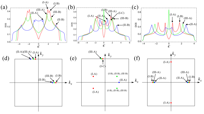
Figure 2: DOS for (a) the model (i), (b) the model (ii), and (c) the model (iii). The positions of the van Hove singularities for (d) the model (i), (e) the model (ii), and (f) the model (iii). For all panels, red, blue, and green lines and points denote the result for the types-I, II, and III, respectively.

Table 1: The tight-binding parameters for the models (i), (ii), and (iii), realizing the types-I, II, and III Dirac fermions.

	$(t,t_{x}^{0},m)$ for model (i)	$(t,t_{x}^{0},m)$ for model (ii)	$(t,t^{\prime},\lambda)$ for model (iii)
Type-I	(-1,-0.3,0.5)	(-1,-0.3,0.7)	(-1,-0.3,0.5)
Type-II	(-1,-1,0.5)	(-1,-1,0.7)	(-1,0.3,1.5)
Type-III	(-1,-0.5,0.5)	(-1,-0.5,0.7)	(-1,-0.3,1)

III Square-lattice tight-binding models for tilted Dirac Hamiltonian

Next, we consider the two-dimensional Dirac Hamiltonian on a square lattice. The following three models are used:

• Model (i): $h^{0}_{\bm{k}}=-2t_{x}^{0}\sin k_{x}$, $h^{x}_{\bm{k}}=t\sin k_{x}$, $h^{y}_{\bm{k}}=t\sin k_{y}$, and $h^{z}_{\bm{k}}=2m(2-\cos k_{x}-\cos k_{y})$.

• Model (ii): $h^{0}_{\bm{k}}=-2t_{x}^{0}\sin k_{x}$, $h^{x}_{\bm{k}}=t\sin k_{x}$, $h^{y}_{\bm{k}}=0$, and $h^{z}_{\bm{k}}=2m(1-\cos k_{x})+2t\cos k_{y}$.

• Model (iii): $h^{0}_{\bm{k}}=2\lambda t^{\prime}(\cos k_{x}-\cos k_{y})$, $h^{x}_{\bm{k}}=2t^{\prime}(\cos k_{x}-\cos k_{y})$, $h^{y}_{\bm{k}}=0$, and $h^{z}_{\bm{k}}=2t(\cos k_{x}+\cos k_{y})$.

The models (i) and (ii) are the two-dimensional analogs of one employed in Ref. 49, and the model (iii) is based on Refs. 44, 48. Note that, among various parameters in the models (i)-(iii), only $\lambda$ is dimensionless and all the others have the dimension of the energy. Note also that we set the lattice constant to be unity. The number of the Dirac points for the models (i), (ii), and (iii) is, respectively, 1, 2, and 4. To be more precise, the Dirac points of the models (i), (ii), and (iii) is, respectively, $\bm{k}=(0,0)$, $\bm{k}=(0,\pm\pi/2)$, and $(\pm\pi/2,\pm\pi/2)$, all of whose energy is 0.

We elaborate on the characteristics of the band structures of the models (i)-(iii). Figure 1 shows the band structures, where the panels (a), (b), and (c) correspond to the models (i), (ii), and (iii), respectively, and those labeled by 1, 2, and 3 correspond to the parameters realizing the Dirac fermions of the types I, II, and III, respectively. The tight-binding parameters are listed in Table 1. As we have mentioned, we see Dirac cones whose numbers are 1, 2, and 4 for the models (i), (ii), and (iii), respectively. By tuning a single parameter, i.e., $t_{x}^{0}$ for the models (i) and (ii) and $\lambda$ for the model (iii), one can control the tilting of the Dirac cones. Among the three models, the model (iii) is characteristic in that, there is a direction where the dispersion is exactly flat for the type-III Dirac fermions, i.e., $k_{x}\pm k_{y}=\pm\pi$. For the other two models, the dispersion is not exactly flat for the type-III Dirac fermions due to the higher-order terms of $\bm{k}$ around the Dirac points.

Figures 2(a), 2(b), and 2(c) show the DOS for the models (i), (ii), and (iii), respectively, in the cases of types I-III. Here the DOS is defined as

$$\rho(\epsilon)=\frac{1}{V}\sum_{\bm{k},\eta=\pm}\frac{\Gamma}{\pi[(\epsilon-\varepsilon_{\bm{k},\eta})^{2}+\Gamma^{2}]},$$ (15)

with $\Gamma$ being the damping rate. We set $\Gamma=0.06$ for consistency to the calculations of the orbital magnetic susceptibility we show later. For all three models, the DOS has a symmetry, $\rho(\epsilon)=\rho(-\epsilon)$, which reflects the symmetry of the band structures. To be specific, $\varepsilon_{-\bm{k},-}=-\varepsilon_{\bm{k},+}$ for the models (i) and (ii), and $\varepsilon_{\bm{k}+(\pi,\pi),-}=-\varepsilon_{\bm{k},+}$ for the model (iii). We also see that the type-I Dirac fermions have a vanishing DOS at the Dirac point (i.e., $\epsilon=0$), while the type-II Dirac fermions have a finite DOS. For the type-III Dirac fermions, the DOS at the Dirac point exhibits a dip-like shape for the model (i), whereas it exhibits a peak-like shape for the models (ii) and (iii).

Away from the Dirac point, we also see in Figs. 2(a)-(c) that there exist several peaks as denoted by the black arrows (only those having the positive energies are marked). They correspond to the van Hove singularities. In Figs. 2(d), 2(e), and 2(f), we depict the corresponding momentum of each van Hove singularity, i.e., the saddle points of the dispersion, for the models (i), (ii), and (iii), respectively.

IV Results 

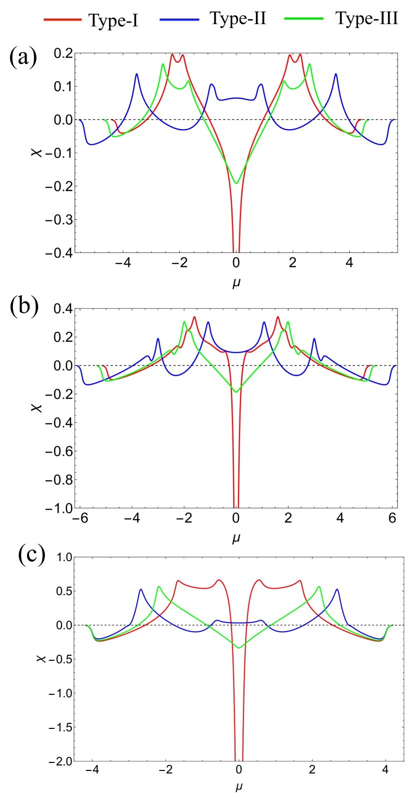
Figure 3: Orbital magnetic susceptibility as a function of $\mu$ at $T=0$. The panels (a), (b), and (c) correspond to the models (i), (ii), and (iii), respectively. Note that the susceptibility is on the vertical axis in the unit of $\frac{e^{2}}{2\pi\hbar^{2}}$.

In this section, we present the numerical results on the orbital magnetic susceptibility for the square-lattice models hosting Dirac cones.

IV.1 Formulation for numerical calculation

For the present models, we calculate the orbital magnetic susceptibility numerically. As for the summation over the Matsubara frequency, we use the standard method to replace it to the energy integral with Fermi distribution function as

$$\chi=-\frac{e^{2}}{2\pi\hbar^{2}}\int_{-\infty}^{\infty}d\epsilon f(\epsilon)\mathrm{Im}[\Theta(\epsilon)],$$ (16)

with

$$\Theta(\epsilon)=\frac{1}{V}\sum_{\bm{k}}\mathrm{Tr}[v^{x}_{\bm{k}}G_{\bm{k}}(\epsilon)v^{y}_{\bm{k}}G_{\bm{k}}(\epsilon)v^{x}_{\bm{k}}G_{\bm{k}}(\epsilon)v^{y}_{\bm{k}}G_{\bm{k}}(\epsilon)].$$ (17)

Here $G_{\bm{k}}(\epsilon)=(\epsilon+i\Gamma-\mathcal{H}_{\bm{k}})^{-1}$ is the retarded Green’s function. Note that $\Gamma$ corresponds to the damping rate. Note also that $\frac{\partial^{2}\mathcal{H}_{\bm{k}}}{\partial k_{x}\partial k_{y}}=0$ holds for the models (i)-(iii). Several groups have shown that the orbital magnetic susceptibility in the lattice model has the form [28]

$$\tilde{\Theta}(\epsilon)=\frac{1}{V} \sum_{\bm{k}}\mathrm{Tr}\biggl{[}v^{x}_{\bm{k}}G_{\bm{k}}(\epsilon)v^{y}_{\bm{k}}G_{\bm{k}}(\epsilon)v^{x}_{\bm{k}}G_{\bm{k}}(\epsilon)v^{y}_{\bm{k}}G_{\bm{k}}(\epsilon)$$ (18)

$$+\frac{1}{2}\bigl{\{}G_{\bm{k}}(\epsilon)v^{x}_{\bm{k}}G_{\bm{k}}v^{y}_{\bm{k}}+G_{\bm{k}}(\epsilon)v^{y}_{\bm{k}}G_{\bm{k}}v^{x}_{\bm{k}}\bigr{\}}G_{\bm{k}}v^{xy}_{\bm{k}}\biggr{]},$$ (19)

or [6]

$$\tilde{\Theta}(\epsilon)=\frac{1}{V}\sum_{\bm{k}} \mathrm{Tr}\biggl{[}\frac{2}{3}v^{x}_{\bm{k}}G_{\bm{k}}(\epsilon)v^{y}_{\bm{k}}G_{\bm{k}}(\epsilon)v^{x}_{\bm{k}}G_{\bm{k}}(\epsilon)v^{y}_{\bm{k}}G_{\bm{k}}(\epsilon)$$ (21)

$$-\frac{2}{3}v^{x}_{\bm{k}}G_{\bm{k}}(\epsilon)v^{x}_{\bm{k}}G_{\bm{k}}(\epsilon)v^{y}_{\bm{k}}G_{\bm{k}}(\epsilon)v^{y}_{\bm{k}}G_{\bm{k}}(\epsilon)$$ (22)

$$+\frac{1}{6}\bigl{\{}v^{xx}_{\bm{k}}G_{\bm{k}}(\epsilon)v^{yy}_{\bm{k}}G_{\bm{k}}-v^{xy}_{\bm{k}}G_{\bm{k}}(\epsilon)v^{xy}_{\bm{k}}G_{\bm{k}}\bigr{\}}\biggr{]},$$ (23)

instead of $\Theta(\epsilon)$ in Eq. (17), where $v^{ij}_{\bm{k}}=\frac{\partial^{2}\mathcal{H}_{\bm{k}}}{\partial k_{i}\partial k_{j}}$. In the present case where $\frac{\partial^{2}\mathcal{H}_{\bm{k}}}{\partial k_{x}\partial k_{y}}=0$ holds, it is apparent that the results using Eq. (LABEL:eq:Gomez_formula) is the same as those using Eq. (17). We also find that Eq. (23) is equivalent to Eq. (17) in the present case as far as the boundary contributions in the integration by parts vanish. (See the appendix B for details.) Therefore, the above three formulae for $\tilde{\Theta}(\epsilon)$ give the same results.

IV.2 Numerical results

Figures 3(a), 3(b), and 3(c) show the $\mu$ dependence of the orbital magnetic susceptibility for the models (i), (ii), and (iii), respectively. Here we set $T=0$ and $\Gamma=0.06$. Focusing on the Dirac point ($\mu=0$), all three models exhibit qualitatively similar behavior. Specifically, we see that the type-I Dirac fermions exhibit divergingly large diamagnetic susceptibility, which coincides with the result in the previous section for the continuum model and the previous works [16, 17, 18, 27, 28, 6, 29]. Meanwhile, the type-II Dirac fermions do not show divergingly large susceptibility. It has a small positive value and the $\mu$ dependence around the Dirac point is very small, which is in sharp contrast to the type-I case where the steep drop of $\chi$ around the Dirac point is seen. Note that in the continuum model in Sec. II.2, the orbital magnetic susceptibility vanishes, meaning that the finite values of $\chi$ obtained here originate from the lattice model. As for the type-III case, we see the diamagnetic susceptibility, but its value is much smaller than that for the type-I. Comparing among three models, we see that the ratio between the orbital magnetic susceptibility of the type-III and the type-I becomes smaller as the number of the Dirac cones increases.

Away from the Dirac points, we see several peaks of $\chi$, all of which are positive-signed (i.e., paramagnetic). We elaborate on the origin of these peaks in the next section.

Figure 4 shows the temperature dependence of $\chi$ with $\mu=0$. Again, qualitative behavior is common among the three models. We see that only the type-I Dirac fermions exhibit steep temperature dependence, namely, the diamagnetic susceptibility becomes larger as $T\rightarrow 0$. In contrast, $\chi$ exhibits a small temperature dependence for the types-II and III Dirac fermions.

Summarizing these results, we find that only the type-I Dirac fermions show characteristic divergingly large diamagnetism at the Dirac points, which has a sharp dependence on $\mu$ and $T$, whereas the type-II Dirac fermions show small paramagnetism which is rather insensitive to $\mu$ and $T$. The type-III fermions show the diamagnetism which is moderately dependent on $\mu$ but rather insensitive to $T$.

V Discussions

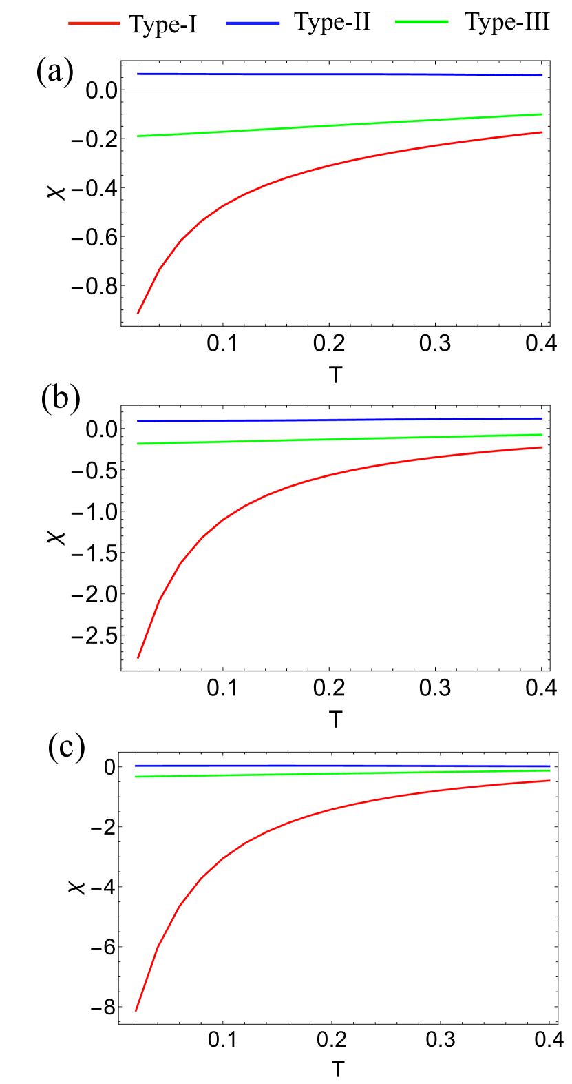
Figure 4: Orbital magnetic susceptibility as a function of $T$ at $\mu=0$. The panels (a), (b), and (c) correspond to the models (i), (ii), and (iii), respectively. $\chi$ in the vertical axis is in the unit of $\frac{e^{2}}{2\pi\hbar^{2}}$.

V.1 Role of Dirac points in type-II case

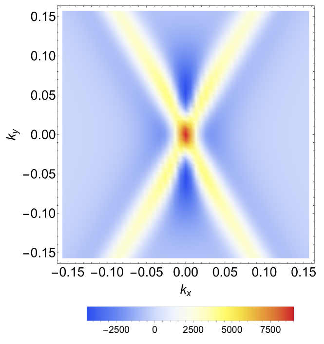
Figure 5: The map of $\bar{\chi}_{\bm{k}}$ for the continuum model of Eq. (6). We set $\alpha=2$, $v_{\rm F}=1$, $\mu=0$, and $\Gamma=0.06$.

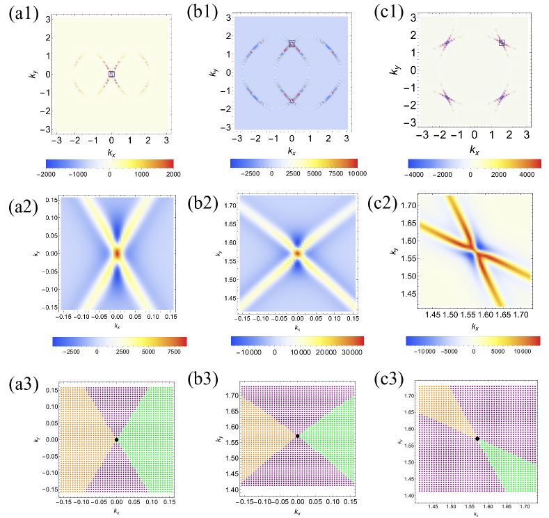
Figure 6: The map of $\bar{\chi}_{\bm{k}}$ of Eq. (24) for the type-II case at $\mu=0$. The panels (a), (b), and (c) are for the models (i), (ii), and (iii), respectively. The upper panels are the map for the entire Brillouin zone. The middle panels are the zoom-up near a Dirac point, i.e., $\bm{k}=(0,0)$ for (a), $(0,\pi/2)$ for (b), and $(\pi/2,\pi/2)$ for (c). The lower panels represent the classification of the regions near the Dirac point with respect to the occupation of the bands. The orange dots represent the region where both upper and the lower bands are occupied. The green dots represent the region where both upper and the lower bands are unoccupied. The purple dots represent the region where only the lower band is occupied.

Unlike the type-I case, in the type-II case, the Fermi surface extends the region away from the Dirac points. Thus, here we argue whether the Dirac points play essential roles for the orbital magnetic susceptibility when the chemical potential is at the Dirac point. To this end, we compute the momentum-resolved contributions to the orbital magnetic susceptibility :

$$\bar{\chi}_{\bm{k}}=-\int_{-\infty}^{\infty}d\epsilon f(\epsilon)\mathrm{Im}[\theta_{\bm{k}}(\epsilon)],$$ (24)

with

$$\theta_{\bm{k}}(\epsilon)=\mathrm{Tr}[v^{x}_{\bm{k}}G_{\bm{k}}(\epsilon)v^{y}_{\bm{k}}G_{\bm{k}}(\epsilon)v^{x}_{\bm{k}}G_{\bm{k}}(\epsilon)v^{y}_{\bm{k}}G_{\bm{k}}(\epsilon)].$$ (25)

First, we examine how the orbital magnetic susceptibility vanishes in the continuum model in the type-II case. We calculate $\bar{\chi}_{\bm{k}}$ using Eqs. (6) and (8) with $\alpha=2$ at $\mu=0$ with $\Gamma=0.06$. As shown in Fig. 5, we can see that there are delta-function-like positive peaks maximized at the Dirac point along $\alpha\cos\theta\pm 1=0$ [$\theta=\tan^{-1}(k_{y}/k_{x})$], which correspond to the Fermi surfaces of the continuum model. On the other hand, in the region where both $\alpha\cos\theta+1>0$ and $\alpha\cos\theta-1<0$ hold (i.e., the region where only the lower band is occupied), there are negative contributions. As pointed out in Eq. (11), the orbital magnetic susceptibility exactly vanishes after performing the integration over $\bm{k}$. Therefore, we expect that the cancellation occurs between the large positive contribution at the Fermi surface and the negative contributions from the other region in the continuum model.

Let us proceed to the lattice models. In Fig. 6, we plot $\bar{\chi}_{\bm{k}}$ for the type-II case at $\mu=0$. The upper panels are the map for the entire Brillouin zone. We see that the main contributions originate from the Fermi surface. The middle panels are the zoom-up near a Dirac point. We see that $\bar{\chi}_{\bm{k}}$ sharply oscillates along the direction perpendicular to the tilting of the cone. To be specific, $\bar{\chi}_{\bm{k}}$ has a large positive value right at the Dirac point, whereas it has a large positive value along the Fermi surfaces and a large negative value in the two areas out of four areas away from the Dirac point. For closer look at this, in the lower panels, we classify the momentum space with respect to the band occupation. There are classified into three types as indicated by the colors. Specifically, the orange (green) dots represent the region where both upper and the lower bands are occupied (unoccupied), and the purple dots represent the region where only the lower band is occupied. As mentioned above, we see that the positive contribution comes from the Fermi surface, maximized at the Dirac point, while the large negative value comes from the region represented by the purple dots. These behaviors are qualitatively the same behavior as in the continuum model shown in Fig. 5. However, the exact cancellation does not occur in the lattice models. As a result of this subtle cancellation, the susceptibility for the type-II case at $\mu=0$ is moderately paramagnetic [Fig. 3]. This is in contrast with the type-I Dirac fermions that contribute divergingly to the diamagnetic susceptibility.

V.2 Comparison to the Landau-Peierls formula

In Sec. I, we have addressed the importance of the interband effect in the orbital magnetic susceptibility. In this regard, it is worth interpreting our results in terms of the intraband versus interband contributions. To extract the intraband contribution in the present results, we employ the Landau-Peierls formula [51, 52] to calculate the orbital magnetic susceptibility that purely comes from the intraband contribution:

$$\chi^{\mathrm{LP}}=\frac{e^{2}}{12\hbar^{2}V}$$

$$\times\sum_{\bm{k},\eta=\pm}\left\{\left(\frac{\partial^{2}\varepsilon_{\bm{k},\eta}}{\partial k_{x}^{2}}\right)\left(\frac{\partial^{2}\varepsilon_{\bm{k},\eta}}{\partial k_{y}^{2}}\right)-\left(\frac{\partial^{2}\varepsilon_{\bm{k},\eta}}{\partial k_{x}\partial k_{y}}\right)^{2}\right\}\frac{\partial f(\varepsilon_{\bm{k},\eta})}{\partial\epsilon}.$$ (26)

We note that the damping rate $\Gamma$ is neglected in this formula, hence we cannot compare the results for $\chi^{\mathrm{LP}}$ with $\chi$ presented in Fig. 3 in a quantitative manner. Nevertheless, we can extract the features of the $\mu$ dependence of $\chi$, as we will show later.

Figure 7 shows the $\chi$ and $\chi^{\rm LP}$ as functions of $\mu$ with $\mu\geq 0$. Note that we set $T=0.06$ in calculating $\chi^{\rm LP}$, so that we can compare $\chi^{\rm LP}$ with $\chi$ at the finite $\Gamma$ in an ad hoc manner. We see that the paramagnetic peaks of $\chi$ can be accounted for by $\chi^{\rm LP}$. As mentioned in Sec. III, the peak positions correspond to the van Hove singularities. Note that the emergence of the paramagnetic peaks at the van Hove singularities coincides with the various two-dimensional tight-binding models such as the single-orbital square lattice [6, 53] and the honeycomb lattice [6, 28, 29].

We also see that $\chi^{\rm LP}$ (dashed lines in Fig. 7) are finite for $\mu\sim 0$, which does not reproduce the behavior of $\chi$ near $\mu=0$ for all three types of the Dirac cones, meaning that the interband contribution plays an essential role, not for the type-I but also for types-II and III.

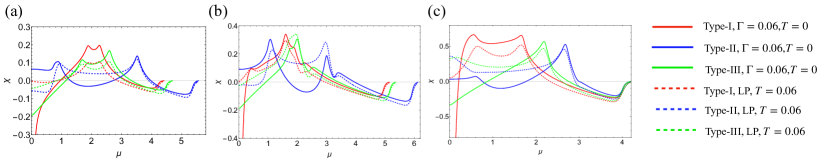
Figure 7: Comparison between the total orbital magnetic susceptibility at $T=0$, $\Gamma=0.06$ (represented by the solid lines) and the Landau-Peierls susceptibility at $T=0.06$ (represented by the dashed lines). Panels (a), (b), and (c) are for the models (i), (ii), and (iii), respectively. Note that the susceptibility is on the vertical axis in the unit of $\frac{e^{2}}{2\pi\hbar^{2}}$.

VI Summary

We have investigated the orbital magnetic susceptibility for the two-dimensional massless Dirac fermions in the continuum model and the lattice models, paying attention to the comparison among types I, II, and III. For studying the lattice models, we have employed three different models, all of which are defined on a square lattice and described by the $2\times 2$ Hamiltonian in the momentum space.

For the continuum model, as is well-known, $\chi$ is diamagnetic and diverging for the type-I, but is proportional to $(1-\alpha)^{3/2}$ (i.e., the divergence is weaken as the tilting increases). In contrast to this, we have clarified that $\chi$ vanishes for the types II and III.

We then compare this behavior with the lattice models. We have found that, in the case where the chemical potential is at the Dirac point, the type-I Dirac fermions exhibit divergingly large diamagnetic susceptibility, the type-II Dirac fermions exhibit finite but small paramagnetic susceptibility, and the type-III Dirac fermions exhibit diamagnetic susceptibility but the divergence is much weaker. This behavior is different from the continuum model, which is attributed to the lattice. As for the temperature dependence, only type-I Dirac fermions show strong temperature dependence, whereas types-II and III are almost temperature-independent. The fact that the qualitative behaviors are in common among the three models indicates that the results are universal among the Dirac fermions for the lattice models. For the type-II case, we have investigated the momentum-resolved contributions to the orbital magnetic susceptibility, and have found that the contribution near the Dirac points sharply oscillates, resulting in a small contribution. Thus, the moderate paramagnetic susceptibility originates from the Fermi surface away from the Dirac points.

We have also found that, away from $\mu=0$ where Dirac points exist, there are several positive-sign peaks of the orbital magnetic susceptibility as a function of $\mu$. They correspond to the van Hove singularity, and can be accounted for the Landau-Peierls-type intraband contributions.

Appendix A Orbital magnetic susceptibility in the massless Dirac Hamiltonian with tilting

In this appendix, we show some details of the calculations of $\chi$ in the two-dimensional Dirac Hamiltonian with tilting. Since $D=(i\tilde{\varepsilon}_{n})^{2}-x^{2}-y^{2}$ with $i\tilde{\varepsilon}_{n}=i\varepsilon_{n}+\alpha x+\mu$, the following relation holds:

$$\frac{\partial}{\partial x}\frac{1}{D^{3}}=\frac{6}{D^{4}}(x-\alpha i\tilde{\varepsilon}_{n}).$$ (27)

We can use this relation in the first term of Eq. (9) to perform the integration by parts. Then, we obtain

$$\chi=e^{2}v_{\rm F}^{2}k_{\rm B}T\sum_{n}\iint\frac{dxdy}{4\pi^{2}}\left[-\frac{4y^{2}(1-\alpha^{2})}{3D^{3}}-\frac{1-\alpha^{2}}{D^{2}}\right].$$ (28)

Note that we have used

$$\frac{4y^{2}(x-\alpha i\tilde{\varepsilon}_{n})}{3D^{3}}\bigg{|}_{x=\pm\infty}=0,$$ (29)

which holds even when $\alpha=1$. Furthermore, using the relation

$$\frac{\partial}{\partial y}\frac{1}{D^{2}}=\frac{4y}{D^{3}},$$ (30)

Eq. (28) becomes

$$\chi=e^{2}v_{\rm F}^{2}k_{\rm B}T\sum_{n}\iint\frac{dxdy}{4\pi^{2}}\left[\frac{1-\alpha^{2}}{3D^{2}}-\frac{1-\alpha^{2}}{D^{2}}\right],$$ (31)

which leads to Eq. (10) in the main text.

Next, we perform the $x$ and $y$ integrals. Using the polar coordinate in two-dimension, we put $x=p\cos\theta$ and $y=p\sin\theta$. Then, Eq. (10) becomes

$$\chi=-\frac{e^{2}v_{\rm F}^{2}}{6\pi^{2}}(1-\alpha^{2})k_{\rm B}T\sum_{n}\int_{0}^{2\pi}d\theta\int_{0}^{\infty}pdp\frac{1}{D_{1}^{2}D_{2}^{2}},$$ (32)

with $D_{1}=i\varepsilon_{n}+\mu+(\alpha\cos{}\theta-1)p$ and $D_{2}=i\varepsilon_{n}+\mu+(\alpha\cos\theta+1)p$. Using

$$\frac{1}{D_{1}D_{2}} =\frac{1}{2p}\left(\frac{1}{D_{1}}-\frac{1}{D_{2}}\right),$$ (33)

$$\frac{1}{pD_{1}} =\frac{1}{D_{0}}\left(\frac{1}{p}-\frac{\alpha\cos\theta-1}{D_{1}}\right),$$ (34)

$$\frac{1}{pD_{2}} =\frac{1}{D_{0}}\left(\frac{1}{p}-\frac{\alpha\cos\theta+1}{D_{2}}\right),$$ (35)

with $D_{0}=i\varepsilon_{n}+\mu$, we can show

$$\frac{p}{D_{1}^{2}D_{2}^{2}}= \frac{1}{4p}\left[\frac{1}{D_{1}^{2}}+\frac{1}{D_{2}^{2}}-\frac{1}{p}\left\{\frac{1}{D_{1}}-\frac{1}{D_{2}}\right\}\right]$$ (36)

$$= -\frac{1}{4D_{0}}\left(\frac{\alpha\cos\theta-1}{D_{1}^{2}}+\frac{\alpha\cos\theta+1}{D_{2}^{2}}\right)$$ (37)

$$-\frac{\alpha\cos\theta}{4D_{0}^{2}}\left(\frac{\alpha\cos\theta-1}{D_{1}}-\frac{\alpha\cos\theta+1}{D_{2}}\right).$$

Using this relation, the $p$-integral in $\chi$ can be carried out, which leads to

$$\chi=\frac{e^{2}v_{\rm F}^{2}}{24\pi^{2}}(1-\alpha^{2})k_{\rm B}T\sum_{n}\frac{1}{D_{0}^{2}}\int_{0}^{2\pi}d\theta F(\theta,\alpha),$$ (39)

with

$$F(\theta,\alpha)=2+\alpha\cos\theta\biggl{[}\frac{1}{2}\ln\frac{(\alpha\cos\theta-1)^{2}}{(\alpha\cos\theta+1)^{2}}$$ (40)

$$-\frac{i\pi}{2}{\rm sign}(\alpha\cos\theta-1)+\frac{i\pi}{2}{\rm sign}(\alpha\cos\theta+1)\biggr{]}.$$ (41)

It is easy to see that the imaginary part in $F(\theta,\alpha)$ does not contribute to $\chi$ even if $\alpha>1$. The integral of the term with logarithm should be carried out with care. When $\alpha<1$, using the integration by parts, we obtain

$$\int_{0}^{2\pi}d\theta\frac{\alpha\cos\theta}{2}\ln\frac{(\alpha\cos\theta-1)^{2}}{(\alpha\cos\theta+1)^{2}}$$ (42)

$$=\alpha\sin\theta\ln\frac{(\alpha\cos\theta-1)^{2}}{(\alpha\cos\theta+1)^{2}}\biggl{|}^{\pi}_{0}+\int_{0}^{\pi}d\theta\left(\frac{2\alpha^{2}\sin^{2}\theta}{\alpha\cos\theta-1}-\frac{2\alpha^{2}\sin^{2}\theta}{\alpha\cos\theta+1}\right)$$ (43)

$$=\int_{0}^{\pi}d\theta\left(-4+\frac{2(\alpha^{2}-1)}{\alpha\cos\theta-1}-\frac{2(\alpha^{2}-1)}{\alpha\cos\theta+1}\right)$$ (44)

$$=-4\pi+4\pi\sqrt{1-\alpha^{2}}.$$ (45)

As a result, $\chi$ becomes

$$\chi=\frac{e^{2}v_{\rm F}^{2}}{6\pi}(1-\alpha^{2})^{3/2}k_{\rm B}T\sum_{n}\frac{1}{D_{0}^{2}},$$ (46)

for $\alpha<1$, which is equivalent to Eq. (11).

On the other hand, when $1<\alpha$, $\alpha\cos\theta-1$ or $\alpha\cos\theta+1$ in the logarithm vanishes when $\theta=\theta_{0}$ where $\theta_{0}$ satisfies $\sin\theta_{0}=\sqrt{\alpha^{2}-1}/\alpha$. To avoid the singularities in the integration by parts, we perform a different integration from (45) as

$$\int_{0}^{2\pi}d\theta\frac{\alpha\cos\theta}{2}\ln\frac{(\alpha\cos\theta-1)^{2}}{(\alpha\cos\theta+1)^{2}}$$ (47)

$$=\left(\alpha\sin\theta-\sqrt{\alpha^{2}-1}\right)\ln\frac{(\alpha\cos\theta-1)^{2}}{(\alpha\cos\theta+1)^{2}}\biggl{|}^{\pi}_{0}$$ (48)

$$+\int_{0}^{\pi}d\theta\left(\alpha\sin\theta-\sqrt{\alpha^{2}-1}\right)\left(\frac{2\alpha\sin\theta}{\alpha\cos\theta-1}-\frac{2\alpha\sin\theta}{\alpha\cos\theta+1}\right)$$ (49)

$$=4\sqrt{\alpha^{2}-1}\ln\frac{\alpha-1}{\alpha+1}-\int_{0}^{\pi}d\theta\frac{4\alpha\sin\theta}{\alpha\sin\theta+\sqrt{\alpha^{2}-1}}$$ (50)

$$=-4\pi.$$ (51)

As a result, $\chi$ vanishes for $\alpha>1$.

Appendix B Equivalence of the two formulae of orbital magnetic susceptibility in Eqs. (17) and (23)

First, we can show that

$$\frac{\partial}{\partial k_{\mu}}G_{\bm{k}}(\epsilon)=G_{\bm{k}}(\epsilon)v_{\bm{k}}^{\mu}G_{\bm{k}}(\epsilon),$$ (52)

with $\mu=x,y$. Using this relation and a trick, we see that

$$\Theta(\epsilon)=\frac{1}{V}\sum_{\bm{k}} \mathrm{Tr}\biggl{[}\frac{2}{3}v^{x}_{\bm{k}}G_{\bm{k}}(\epsilon)v^{y}_{\bm{k}}G_{\bm{k}}(\epsilon)v^{x}_{\bm{k}}G_{\bm{k}}(\epsilon)v^{y}_{\bm{k}}G_{\bm{k}}(\epsilon)$$ (53)

$$+\frac{1}{3}v^{x}_{\bm{k}}\left(\frac{\partial}{\partial k_{y}}G_{\bm{k}}(\epsilon)\right)v^{x}_{\bm{k}}G_{\bm{k}}(\epsilon)v^{y}_{\bm{k}}G_{\bm{k}}(\epsilon)\biggr{]}.$$ (54)

Then, we perform the integration by parts in the second term assuming that the boundary contributions of the Brillouin zone vanish. For lattice models, the vanishing of the surface terms can be proven [54]. Furthermore, in the case where $v_{\bm{k}}^{xy}=0$ holds, the second term becomes

$$\frac{1}{V}\sum_{\bm{k}}\mathrm{Tr}\biggl{[} -\frac{2}{3}v^{x}_{\bm{k}}G_{\bm{k}}(\epsilon)v^{x}_{\bm{k}}G_{\bm{k}}(\epsilon)v^{y}_{\bm{k}}G_{\bm{k}}(\epsilon)v^{y}_{\bm{k}}G_{\bm{k}}(\epsilon)$$ (55)

$$-\frac{1}{3}v^{x}_{\bm{k}}G_{\bm{k}}(\epsilon)v^{x}_{\bm{k}}G_{\bm{k}}(\epsilon)v^{yy}_{\bm{k}}G_{\bm{k}}\biggr{]}.$$ (56)

In the similar way, the second term in Eq. (56) can be transformed as

$$\frac{1}{V}\sum_{\bm{k}}\mathrm{Tr}\biggl{[}-\frac{1}{3}v^{x}_{\bm{k}}\left(\frac{\partial}{\partial k_{x}}G_{\bm{k}}(\epsilon)\right)v^{yy}_{\bm{k}}G_{\bm{k}}\biggr{]}$$ (57)

$$= \frac{1}{V}\sum_{\bm{k}}\mathrm{Tr}\biggl{[}\frac{1}{3}v^{x}_{\bm{k}}G_{\bm{k}}(\epsilon)v^{yy}_{\bm{k}}G_{\bm{k}}(\epsilon)v_{\bm{k}}^{x}G_{\bm{k}}(\epsilon)$$ (58)

$$+\frac{1}{3}v^{xx}_{\bm{k}}G_{\bm{k}}(\epsilon)v^{yy}_{\bm{k}}G_{\bm{k}}(\epsilon)\biggr{]}.$$ (59)

The first term on the right-hand side is the same as the left-hand side by using the cyclic nature of the trace. As a result, we can see that the second term in Eq. (56) is equal to

$$\frac{1}{V}\sum_{\bm{k}}\mathrm{Tr}\biggl{[}\frac{1}{6}v^{xx}_{\bm{k}}G_{\bm{k}}(\epsilon)v^{yy}_{\bm{k}}G_{\bm{k}}(\epsilon)\biggr{]}.$$ (60)

Combining the above formulae, we can see that Eq. (23) gives the same result with Eq. (17) because $v_{\bm{k}}^{xy}=0$.

References

- Blount [1962] E. I. Blount, Phys. Rev. 126, 1636 (1962).
- Fukuyama and Kubo [1969] H. Fukuyama and R. Kubo, Journal of the Physical Society of Japan 27, 604 (1969).
- Fukuyama [1971] H. Fukuyama, Progress of Theoretical Physics 45, 704 (1971).
- Ogata and Fukuyama [2015] M. Ogata and H. Fukuyama, Journal of the Physical Society of Japan 84, 124708 (2015).
- Raoux et al. [2014] A. Raoux, M. Morigi, J.-N. Fuchs, F. Piéchon, and G. Montambaux, Phys. Rev. Lett. 112, 026402 (2014).
- Raoux et al. [2015] A. Raoux, F. Piéchon, J.-N. Fuchs, and G. Montambaux, Phys. Rev. B 91, 085120 (2015).
- Gao et al. [2015] Y. Gao, S. A. Yang, and Q. Niu, Phys. Rev. B 91, 214405 (2015).
- Piéchon et al. [2016] F. Piéchon, A. Raoux, J.-N. Fuchs, and G. Montambaux, Phys. Rev. B 94, 134423 (2016).
- Ogata [2017] M. Ogata, Journal of the Physical Society of Japan 86, 044713 (2017).
- Rhim et al. [2020] J.-W. Rhim, K. Kim, and B.-J. Yang, Nature 584, 59 (2020).
- Ozaki and Ogata [2021] S. Ozaki and M. Ogata, Phys. Rev. Res. 3, 013058 (2021).
- Ozaki and Ogata [2023] S. Ozaki and M. Ogata, Phys. Rev. B 107, 085201 (2023).
- [13] S. Ozaki, H. Matsuura, I. Tateishi, T. Koretsune, and M. Ogata, arXiv: 2406.07281.
- Shoenberg et al. [1936] D. Shoenberg, M. Z. Uddin, and E. Rutherford, Proceedings of the Royal Society of London. Series A - Mathematical and Physical Sciences 156, 687 (1936).
- Ganguli and Krishnan [1941] N. Ganguli and K. S. Krishnan, Proceedings of the Royal Society of London. Series A. Mathematical and Physical Sciences 177, 168 (1941).
- McClure [1956] J. W. McClure, Phys. Rev. 104, 666 (1956).
- McClure [1960] J. W. McClure, Phys. Rev. 119, 606 (1960).
- Koshino and Ando [2007a] M. Koshino and T. Ando, Phys. Rev. B 75, 235333 (2007a).
- Koshino and Ando [2007b] M. Koshino and T. Ando, Phys. Rev. B 76, 085425 (2007b).
- Nakamura [2007] M. Nakamura, Phys. Rev. B 76, 113301 (2007).
- Koshino and Ando [2010] M. Koshino and T. Ando, Phys. Rev. B 81, 195431 (2010).
- Koshino and Ando [2011] M. Koshino and T. Ando, Solid State Communications 151, 1054 (2011), graphene.
- Fuseya et al. [2015] Y. Fuseya, M. Ogata, and H. Fukuyama, Journal of the Physical Society of Japan 84, 012001 (2015).
- Watanabe et al. [2021] Y. Watanabe, M. Kumazaki, H. Ezure, T. Sasagawa, R. Cava, M. Itoh, and Y. Shimizu, Journal of the Physical Society of Japan 90, 053701 (2021).
- Suetsugu et al. [2021] S. Suetsugu, K. Kitagawa, T. Kariyado, A. W. Rost, J. Nuss, C. Mühle, M. Ogata, and H. Takagi, Phys. Rev. B 103, 115117 (2021).
- Fujiyama et al. [2022] S. Fujiyama, H. Maebashi, N. Tajima, T. Tsumuraya, H.-B. Cui, M. Ogata, and R. Kato, Phys. Rev. Lett. 128, 027201 (2022).
- Kobayashi et al. [2008] A. Kobayashi, Y. Suzumura, and H. Fukuyama, Journal of the Physical Society of Japan 77, 064718 (2008).
- Gómez-Santos and Stauber [2011] G. Gómez-Santos and T. Stauber, Phys. Rev. Lett. 106, 045504 (2011).
- Ogata [2016a] M. Ogata, Journal of the Physical Society of Japan 85, 104708 (2016a).
- Bustamante et al. [2021] J. V. Bustamante, N. J. Wu, C. Fermon, M. Pannetier-Lecoeur, T. Wakamura, K. Watanabe, T. Taniguchi, T. Pellegrin, A. Bernard, S. Daddinounou, V. Bouchiat, S. Guéron, M. Ferrier, G. Montambaux, and H. Bouchiat, Science 374, 1399 (2021).
- Soluyanov et al. [2015] A. A. Soluyanov, D. Gresch, Z. Wang, Q. Wu, M. Troyer, X. Dai, and B. A. Bernevig, Nature 527, 495 (2015).
- Sun et al. [2015] Y. Sun, S.-C. Wu, M. N. Ali, C. Felser, and B. Yan, Phys. Rev. B 92, 161107 (2015).
- Xu et al. [2015] Y. Xu, F. Zhang, and C. Zhang, Phys. Rev. Lett. 115, 265304 (2015).
- Yu et al. [2016] Z.-M. Yu, Y. Yao, and S. A. Yang, Phys. Rev. Lett. 117, 077202 (2016).
- Ruan et al. [2016] J. Ruan, S.-K. Jian, H. Yao, H. Zhang, S.-C. Zhang, and D. Xing, Nature Communications 7, 11136 (2016).
- Volovik [2016] G. E. Volovik, JETP Letters 104, 645 (2016).
- Liu et al. [2018] H. Liu, J.-T. Sun, C. Cheng, F. Liu, and S. Meng, Phys. Rev. Lett. 120, 237403 (2018).
- Huang et al. [2018] H. Huang, K.-H. Jin, and F. Liu, Phys. Rev. B 98, 121110 (2018).
- Fragkos et al. [2019] S. Fragkos, R. Sant, C. Alvarez, E. Golias, J. Marquez-Velasco, P. Tsipas, D. Tsoutsou, S. Aminalragia-Giamini, E. Xenogiannopoulou, H. Okuno, G. Renaud, O. Rader, and A. Dimoulas, Phys. Rev. Materials 3, 104201 (2019).
- Milićević et al. [2019] M. Milićević, G. Montambaux, T. Ozawa, O. Jamadi, B. Real, I. Sagnes, A. Lemaître, L. Le Gratiet, A. Harouri, J. Bloch, and A. Amo, Phys. Rev. X 9, 031010 (2019).
- Kim et al. [2020] J. Kim, S. Yu, and N. Park, Phys. Rev. Applied 13, 044015 (2020).
- Chen et al. [2020] Y.-G. Chen, X. Luo, F.-Y. Li, B. Chen, and Y. Yu, Phys. Rev. B 101, 035130 (2020).
- Jin et al. [2020] L. Jin, H. C. Wu, B.-B. Wei, and Z. Song, Phys. Rev. B 101, 045130 (2020).
- Mizoguchi and Hatsugai [2020] T. Mizoguchi and Y. Hatsugai, Journal of the Physical Society of Japan 89, 103704 (2020).
- Schober et al. [2012] G. A. H. Schober, H. Murakawa, M. S. Bahramy, R. Arita, Y. Kaneko, Y. Tokura, and N. Nagaosa, Phys. Rev. Lett. 108, 247208 (2012).
- Suzumura et al. [2019] Y. Suzumura, T. Tsumuraya, R. Kato, H. Matsuura, and M. Ogata, Journal of the Physical Society of Japan 88, 124704 (2019).
- Note [1] See Supplemental Material of Ref. \rev@citealpSchober2012.
- Mizoguchi et al. [2022] T. Mizoguchi, H. Matsuura, and M. Ogata, Phys. Rev. B 105, 205203 (2022).
- Udagawa and Bergholtz [2016] M. Udagawa and E. J. Bergholtz, Phys. Rev. Lett. 117, 086401 (2016).
- Note [2] Note that is not divided by the volume.
- Landau [1930] L. Landau, Zeitschrift für Physik 64, 629 (1930).
- Peierls [1933] R. Peierls, Zeitschrift für Physik 80, 763 (1933).
- Ogata [2016b] M. Ogata, Journal of the Physical Society of Japan 85, 064709 (2016b).
- Mizoguchi and Okuma [2024] T. Mizoguchi and N. Okuma, Journal of the Physical Society of Japan 93, 095002 (2024).