On the Quantum K-theory of Quiver Varieties at Roots of Unity

Abstract.

Let $\Psi(\mathbold{z},\mathbold{a},q)$ be the fundamental solution matrix of the quantum difference equation in the equivariant quantum K-theory for Nakajima variety $X$. In this work, we prove that the operator

$$\Psi(\mathbold{z},\mathbold{a},q)\Psi\left(\mathbold{z}^{p},\mathbold{a}^{p},q^{p^{2}}\right)^{-1}$$

has no poles at the primitive complex $p$-th roots of unity $\zeta_{p}$ in the curve counting parameter $q$. As a byproduct, we show that the eigenvalues of the iterated product of the operators ${\bf M}_{\mathcal{L}}$ from the quantum difference equation on $X$

$${\bf M}_{\mathcal{L}}(\mathbold{z},\mathbold{a},q){\bf M}_{\mathcal{L}}(\mathbold{z}q^{\mathcal{L}},\mathbold{a},q)\cdots{\bf M}_{\mathcal{L}}(\mathbold{z}q^{(p-1)\mathcal{L}},\mathbold{a},q)$$

evaluated at $\zeta_{p}$ are described by the Bethe equations for $X$ in which all variables are substituted by their $p$-th powers.

Finally, upon a reduction of the quantum difference equation on $X$ to the quantum differential equation over the field with finite characteristic, the above iterated product transforms into a Grothendiek-Katz $p$-curvature of the corresponding differential connection whereas ${\bf M}_{\mathcal{L}}(\mathbold{z}^{p},\mathbold{a}^{p},q^{p})$ becomes a certain Frobenius twist of that connection. In this way, we are reproducing, in part, the statement of a theorem by Etingof and Varchenko.

1. Preliminaries

1.1. Qunatum Difference Equation

Enumerative algebraic geometry (quantum K-theory) of Nakajima varieties is governed by the quantum difference equations (QDE) [Okounkov:2022aa] which take the following form

(1.1) $$\Psi(\mathbold{z}q^{\mathcal{L}},\mathbold{a},q)\mathcal{L}={\bf M}_{\mathcal{L}}(\mathbold{z},\mathbold{a},q)\Psi(\mathbold{z},\mathbold{a},q),\ \ \ \mathcal{L}\in\mathrm{Pic}(X)$$

where $\mathrm{Pic}(X)\cong\mathbb{Z}^{l}$ is the lattice of line bundles on a Nakajima variety $X$ and $l$ denotes the number of vertices in the corresponding quiver. The variables $\mathbold{z}=(z_{1},\dots,z_{l})$ and $\mathbold{a}=(a_{1},\dots,a_{m})$ denote the Kähler and the equivariant parameters respectively. The shift of the Kähler variables is of the form

$$\mathbold{z}q^{\mathcal{L}}=(z_{1}q^{c_{1}},\dots,z_{l}q^{c_{l}})$$

where $c_{i}\in\mathbb{Z}$ are integers determined by

(1.2) $$\mathcal{L}=L_{1}^{c_{1}}\otimes\dots\otimes L_{l}^{c_{l}}$$

where $L_{i}$ denote the generators of $\mathrm{Pic}(X)$ given by tautological line bundles.

The fundamental solution matrix $\Psi(\mathbold{z},\mathbold{a},q)$ is given by a power series in $z$ and is uniquely determined by the normalization

(1.3) $$\Psi(\mathbold{z},\mathbold{a},q)=1+\sum\limits_{d\in H_{2}(X,\mathbb{Z})_{\textrm{eff}}}\Psi_{d}(\mathbold{a},q)\mathbold{z}^{d}\in K_{T}(X)[[z]]$$

The matrix $\Psi(\mathbold{z},\mathbold{a},q)$ provides the capping operator – the fundamental object in enumerative geometry which can be defined as the partition function of quasimaps with relative and non-singular boundary conditions, see Section 7.4 in [Okounkov:2015aa] for definitions.

Consistency of QDE implies that for any two line bundles $\mathcal{L}_{1},\mathcal{L}_{2}\in\mathrm{Pic}(X)$ we have

(1.4) $${\bf M}_{\mathcal{L}_{1}\mathcal{L}_{2}}(\mathbold{z},\mathbold{a},q)={\bf M}_{\mathcal{L}_{2}}(\mathbold{z}q^{\mathcal{L}_{1}},\mathbold{a},q){\bf M}_{\mathcal{L}_{1}}(\mathbold{z},\mathbold{a},q)={\bf M}_{\mathcal{L}_{1}}(\mathbold{z}q^{\mathcal{L}_{2}},\mathbold{a},q){\bf M}_{\mathcal{L}_{2}}(\mathbold{z},\mathbold{a},q)$$

Explicit formulas for ${\bf M}_{\mathcal{L}}(\mathbold{z},\mathbold{a},q)$ in terms of representation theory of quantum groups were obtained in [Okounkov:2022aa]. An alternative description of these operators in terms of the elliptic stable envelope classes were also obtained in [2020arXiv200407862K, Kononov:2020cux]. In any chosen basis of equivariant $K$-theory $K_{T}(X)$ the operators ${\bf M}_{\mathcal{L}}(\mathbold{z},\mathbold{a},q)$ are represented by matrices with coefficients given by rational functions of all parameters $\mathbold{z},\mathbold{a}$ and $q$. It is also known that ${\bf M}_{\mathcal{L}}(\mathbold{z},\mathbold{a},q)$ are nonsingular at any $q\in\mathbb{C}$.

1.2. Limit $q\longrightarrow 1$

Let us consider the following operators

(1.5) $$\mathcal{M}_{\mathcal{L}}(\mathbold{z},\mathbold{a})=\left.{\bf M}_{\mathcal{L}}(\mathbold{z},\mathbold{a},q)\right|_{q=1}.$$

From (1.4) we see that

$$\mathcal{M}_{\mathcal{L}_{1}\mathcal{L}_{2}}(\mathbold{z},\mathbold{a})=\mathcal{M}_{\mathcal{L}_{1}}(\mathbold{z},\mathbold{a})\mathcal{M}_{\mathcal{L}_{2}}(\mathbold{z},\mathbold{a})=\mathcal{M}_{\mathcal{L}_{2}}(\mathbold{z},\mathbold{a})\mathcal{M}_{\mathcal{L}_{1}}(\mathbold{z},\mathbold{a})$$

i.e. these operators commute

(1.6) $$[\mathcal{M}_{\mathcal{L}_{1}}(\mathbold{z},\mathbold{a}),\mathcal{M}_{\mathcal{L}_{2}}(\mathbold{z},\mathbold{a})]=0,\ \ \ \forall\mathcal{L}_{1},\mathcal{L}_{2}\in\mathrm{Pic}(X)\,.$$

In [Pushkar:2016qvw, Koroteev:2017aa] we showed that $\mathcal{M}_{\mathcal{L}}(\mathbold{z},\mathbold{a})$ are the operators of quantum multiplication by $\mathcal{L}$ in the equivariant quantum K-theory ring $QK_{T}(X)$. This ring is commutative which agrees with (1.6).

An interesting problem is to describe the joint set of eigenvalues of the operators $\mathcal{M}_{\mathcal{L}}(\mathbold{z},\mathbold{a})$. It is expected that the spectrum is simple meaning that the common eigenspaces of all $\mathcal{M}_{\mathcal{L}}(\mathbold{z},\mathbold{a})$ are one-dimensional. Among other things the simplicity implies that $\mathcal{M}_{\mathcal{L}}(\mathbold{z},\mathbold{a})$ generate the quantum K-theory ring $QK_{T}(X)$ – the operators of quantum multiplication by any K-theory class can be expressed as a polynomial in $\mathcal{M}_{\mathcal{L}}(\mathbold{z},\mathbold{a})$, $\mathcal{L}\in\mathrm{Pic}(X)$ with certain rational coefficients in $\mathbold{z}$ and $\mathbold{a}$.

1.3. Bethe Ansatz

The above-mentioned eigenvalue problem arises in the theory of quantum integrable spin chains [Pushkar:2016qvw, Koroteev:2017aa]. For any quiver variety $X$ one can study action of a quantum group $\mathcal{U}_{\hbar}(\widehat{\mathfrak{g}}_{X})$ on its K-theory $K_{T}(X)$. This action identifies $K_{T}(X)$ with the quantum Hilbert space of a certain XXZ-type spin chain. In this setting, the algebra of commuting Hamiltonians of the spin chain is identified with the algebra generated by operators of quantum multiplication by K-theory classes. In particular, $\mathcal{M}_{\mathcal{L}}(\mathbold{z},\mathbold{a})$ represents certain Hamiltonians of the corresponding XXZ spin chain. Namely, the operators of quantum multiplication by line bundles $\mathcal{M}_{\mathcal{L}}(\mathbold{z},\mathbold{a})$ appear as the “top” coefficients in of Baxter $Q$-operators of the spin chain [Pushkar:2016qvw]. A classical problem of quantum mechanics aims to describe the the eigenvalues and eigenvectors of the Hamiltonians.

The algebraic Bethe Ansatz [Faddeev:1996iy] is a method used in the theory of integrable models to diagonalize spin chain Hamiltonians. Let $\mathcal{V}_{i}$, $i=1,\dots,l$ be a set of the tautological bundles over a Nakajima variety $X$. Let $\mathbold{x}=\{x_{i,j}\}$ denote the collection of the Grothendieck roots of this vector bundles:

(1.7) $$\mathcal{V}_{i}=x_{i,1}+\dots+x_{i,r_{i}},\ \ r_{i}=\textrm{rk}{\mathcal{V}_{i}}$$

The tautological line bundles are given by $L_{i}=\det\mathcal{V}_{i}=x_{i,1}\cdot\dots\cdot x_{i,r_{i}}$. By (1.2) every line bundle $\mathcal{L}$ can be represented as a certain product of the Grothendieck roots

(1.8) $$\mathcal{L}=\prod_{i,j}\,x_{i,j}$$

The algebraic Bethe Ansatz states that the eigenvalues of $\mathcal{M}_{\mathcal{L}}(\mathbold{z},\mathbold{a})$ are given by the same product

(1.9) $$\lambda(\mathbold{a},\mathbold{z})=\prod_{i,j}\,x_{i,j}$$

where $x_{i,j}$ are now certain functions of $\mathbold{z}$ and $\mathbold{a}$ determined as roots of algebraic equations, known as the Bethe equations:

(1.10) $$\mathfrak{B}(\mathbold{x},\mathbold{z},\mathbold{a})=0.$$

The above equations can be explicitly written using the data of the underlying quiver [Aganagic:2017be], as we shall recall in Section 3. In essence, each solution to the Bethe equations (1.10) provides values for $x_{i,j}$ as specific functions of the parameters $\mathbold{z}$ and $\mathbold{a}$. Substituting those values into (1.10) gives an eigenvalue of $\mathcal{M}_{\mathcal{L}}(\mathbold{z},\mathbold{a})$. All eigenvalues appear in this way.

1.4. Limit $q^{p}\longrightarrow 1$

Let $p\in\mathbb{N}$ and let $\zeta_{p}\in\mathbb{C}$ be a primitive $p$-th root of unity. Let us define the following iterated product of operators ${\bf M}_{\mathcal{L}}(\mathbold{z},\mathbold{a},q)$ from (1.1)

(1.11) $${\bf M}_{\mathcal{L}\,\zeta_{p}}(\mathbold{z},\mathbold{a},q)={\bf M}_{\mathcal{L}}(\mathbold{z},\mathbold{a},q){\bf M}_{\mathcal{L}}(\mathbold{z}q^{\mathcal{L}},\mathbold{a},q){\bf M}_{\mathcal{L}}(\mathbold{z}q^{2\mathcal{L}},\mathbold{a},q)\cdots{\bf M}_{\mathcal{L}}(\mathbold{z}q^{(p-1)\mathcal{L}},\mathbold{a},q)\,,$$

as well as its evaluation at $\zeta_{p}$

(1.12) $$\mathcal{M}_{\mathcal{L},\zeta_{p}}(\mathbold{z},\mathbold{a})={\bf M}_{\mathcal{L}\,\zeta_{p}}(\mathbold{z},\mathbold{a},\zeta_{p})\,.$$

In is evident from (1.4) that

$$\mathcal{M}_{\mathcal{L}_{1}\mathcal{L}_{2},\,\zeta_{p}}(\mathbold{z},\mathbold{a})=\mathcal{M}_{\mathcal{L}_{1}\,\zeta_{p}}(\mathbold{z},\mathbold{a})\mathcal{M}_{\mathcal{L}_{2}\,\zeta_{p}}(\mathbold{z},\mathbold{a})=\mathcal{M}_{\mathcal{L}_{2}\,\zeta_{p}}(\mathbold{z},\mathbold{a})\mathcal{M}_{\mathcal{L}_{1}\,\zeta_{p}}(\mathbold{z},\mathbold{a})$$

In particular, these operators commute

$$[\mathcal{M}_{\mathcal{L}_{1}\,\zeta_{p}}(\mathbold{z},\mathbold{a}),\mathcal{M}_{\mathcal{L}_{2}\,\zeta_{p}}(\mathbold{z},\mathbold{a})]=0,\ \ \ \forall\mathcal{L}_{1},\mathcal{L}_{2}\in\mathrm{Pic}(X).$$

It is therefore natural to study the joint set of eigenvalues for these operators. Our first goal in this paper is to show that the eigenvalues of $\mathcal{M}_{\mathcal{L},\zeta_{p}}(\mathbold{z},\mathbold{a})$ can be obtained from the eigenvalues of quantum operators $\mathcal{M}_{\mathcal{L}}(\mathbold{z},\mathbold{a})$ by raising all parameters to the $p$-th power.

Theorem 1.1.

Let $\{\lambda_{1}(\mathbold{z},\mathbold{a}),\lambda_{2}(\mathbold{z},\mathbold{a}),\dots\}$ be the set of eigenvalues of $\mathcal{M}_{\mathcal{L}}(\mathbold{z},\mathbold{a})$ then the eigenvectors of $\mathcal{M}_{\mathcal{L}\,\zeta_{p}}(\mathbold{z},\mathbold{a})$ are given by the set $\{\lambda_{1}(\mathbold{z}^{p},\mathbold{a}^{p}),\lambda_{2}(\mathbold{z}^{p},\mathbold{a}^{p}),\dots\}$ where $\lambda_{i}(\mathbold{z}^{p},\mathbold{a}^{p})$ is the eigenvalue $\lambda_{i}(z,a)$ in which all Kähler variables $\mathbold{z}=(z_{1},\dots,z_{l})$ and equivariant variables $\mathbold{a}=(a_{1},\dots,a_{m})$ are substituted by $\mathbold{z}^{p}=(z^{p}_{1},\dots,z^{p}_{l})$ and $\mathbold{a}^{p}=(a^{p}_{1},\dots,a^{p}_{m})$ respectively.

We note also that the eigenvalues do not depend on the choice of a primitive root $\zeta_{p}$.

1.5. Lift of the Frobenius Intertwiner

Theorem 1.1 is a corollary of the following pole cancellation property of the fundamental solution matrix $\Psi(\mathbold{z},\mathbold{a},q)$. The coefficients of power series expansion (1.3) have poles in $q$ located at the roots of unity. In particular, $\Psi(\mathbold{z},\mathbold{a},q)$ is singular as $q\longrightarrow\zeta_{p}$.

Let $\Psi(\mathbold{z}^{p},\mathbold{a}^{p},q^{p^{2}})$ be the fundamental solution matrix in which all Kähler and equivariant parameters are raised to power $p$ and the variable $q$ is raised to the power $p^{2}$. We prove the following pole-cancellation property

Theorem 1.2.

The operator

$$\Psi(\mathbold{z},\mathbold{a},q)\Psi\left(\mathbold{z}^{p},\mathbold{a}^{p},q^{p^{2}}\right)^{-1}$$

has no poles in $q$ at primitive $p$-th roots of unity.

Let us define

(1.13) $$\mathsf{F}(\mathbold{z},\mathbold{a},\zeta_{p})=\Psi(\mathbold{z},\mathbold{a},q)\Psi(\mathbold{z}^{p},\mathbold{a}^{p},q^{p^{2}})^{-1}\Big{|}_{q=\zeta_{p}}$$

It follows from the difference equation (1.1) that

(1.14) $$\mathsf{F}(\mathbold{z},\mathbold{a},\zeta_{p})\mathcal{M}_{\mathcal{L}}(\mathbold{z}^{p},\mathbold{a}^{p})\mathsf{F}(\mathbold{z},\mathbold{a},\zeta_{p})^{-1}=\mathcal{M}_{\mathcal{L},\zeta_{p}}(\mathbold{z},\mathbold{a})$$

where $\mathcal{M}_{\mathcal{L}}(\mathbold{z}^{p},\mathbold{a}^{p})$ denotes the operator of quantum multiplication (1.5) in which all variables are raised to power $p$. Theorem 1.1 will follow as an obvious corollary to (1.14).

The operator (1.13) is expected to play a role of the K-theoretic lift of a Frobenius intertwiner [Smirnov:2024yqs].

1.6. Example $T^{*}\mathbb{P}^{1}$

It might be instructive to illustrate the statement of Theorem 1.1 in a simplest example. Consider a Nakajima variety given by the cotangent bundle on the projective line $X=T^{*}\mathbb{P}^{1}$. Let $T\cong(\mathbb{C}^{\times})^{3}$ be a torus with coordinates $\mathbold{a}=(a_{1},a_{2},\hbar)$. We consider the action of $T$ on $X$ induced by the natural action on $\mathbb{C}^{2}$:

$$(x,y)\mapsto(xa_{1},ya_{2})$$

In addition, $T$ acts on $X$ by dilating the cotangent direction by $\hbar^{-2}$, i.e. $\hbar^{2}$ is the weight of the canonical symplectic form on $X$.

The Picard group of this variety is the lattice $\mathrm{Pic}(X)\cong\mathbb{Z}$ generated by the tautological line bundle $\mathcal{L}=\mathcal{O}(1)$. The equivariant $K$-theory is isomorphic to the following ring:

$$K_{T}(X)\cong\mathbb{C}[\mathcal{L},a_{1},a_{2},\hbar]/I_{0}$$

where $I_{0}$ denotes the ideal generated by a single relation

$$(\mathcal{L}-a_{1})(\mathcal{L}-a_{2})=0.$$

The quantum K-theory ring of $X$ is a deformation of this ring:

$$QK_{T}(X)=\mathbb{C}[\mathcal{L},a_{1},a_{2},\hbar][[z]]/I_{z}$$

where $I_{z}$ is the ideal generated by the relation [Okounkov:2022aa, Pushkar:2016qvw]

(1.15) $$(\mathcal{L}-a_{1})(\mathcal{L}-a_{2})=z\hbar^{2}(\mathcal{L}-a_{1}\hbar^{-2})(\mathcal{L}-a_{2}\hbar^{-2}).$$

Specializing $QK_{T}(X)$ at $z=0$ gives classical K-theory $K_{T}(X)$.

The quantum difference equation for $X$ was considered in details in Section 6 of [Okounkov:2022aa], in particular, the explicit expression for the operator $\mathbf{M}_{\mathcal{L}}(z)$ is given in Section 6.3.9. In the stable basis of $K_{T}(X)$ this operator has the form:

$$\mathbf{M}_{\mathcal{L}}(z/q)=\left[\begin{array}[]{cc}{\dfrac{a_{{1}}\left(z-1\right)}{{\hbar}^{2}z-1}}&{\dfrac{a_{{2}}z(\hbar^{-1}-{\hbar})}{{\hbar}^{2}z-1}}\\ \vskip 6.0pt plus 2.0pt minus 2.0pt\cr{\dfrac{a_{{1}}({\hbar}^{-1}-\hbar)}{{\hbar}^{2}z-1}}&{\dfrac{a_{{2}}\left(z-1\right)}{{\hbar}^{2}z-1}}\end{array}\right].$$

In particular, after a rescaling of $z$ this operator becomes independent on $q$. At $q=1$ we obtain the operator of quantum multiplication by $\mathcal{L}$ in $QK_{T}(X)$ in the stable basis:

(1.16) $$\mathcal{M}_{\mathcal{L}}(z)=\left[\begin{array}[]{cc}{\dfrac{a_{{1}}\left(z-1\right)}{{\hbar}^{2}z-1}}&{\dfrac{a_{{2}}z(\hbar^{-1}-{\hbar})}{{\hbar}^{2}z-1}}\\ \vskip 6.0pt plus 2.0pt minus 2.0pt\cr{\dfrac{a_{{1}}({\hbar}^{-1}-\hbar)}{{\hbar}^{2}z-1}}&{\dfrac{a_{{2}}\left(z-1\right)}{{\hbar}^{2}z-1}}\end{array}\right]$$

It is straightforward to check that this matrix satisfies quadratic relation (1.15)

(1.17) $$(\mathcal{M}_{\mathcal{L}}(z)-a_{1})(\mathcal{M}_{\mathcal{L}}(z)-a_{2})-z\hbar^{2}(\mathcal{M}_{\mathcal{L}}(z)-a_{1}\hbar^{-2})(\mathcal{M}_{\mathcal{L}}(z)-a_{2}\hbar^{-2})=0$$

which is nothing but the characteristic polynomial for the matrix $\mathcal{M}_{\mathcal{L}}(z)$.

Next, let $p\in\mathbb{N}$ and $\zeta_{p}$ be a primitive complex root of unity order $p$. Let us consider the operator (1.12). Since in this case $\mathbf{M}_{\mathcal{L}}(z)$ trivially depends on $q$ we have

$$\mathcal{M}_{\mathcal{L},\zeta_{p}}(z,a)=\mathcal{M}_{\mathcal{L}}(z)\mathcal{M}_{\mathcal{L}}(z\zeta_{p})\mathcal{M}_{\mathcal{L}}(z\zeta_{p}^{2})\cdots\mathcal{M}_{\mathcal{L}}(z\zeta_{p}^{p-1})$$

One can verify that for any choice of $p$ and $\zeta_{p}$ this matrix satisfies the following relation

(1.18) $$(\mathcal{M}_{\mathcal{L},\zeta_{p}}(z,a)-a_{1}^{p})(\mathcal{M}_{\mathcal{L},\zeta_{p}}(z,a)-a^{p}_{2})-z^{p}\hbar^{2p}(\mathcal{M}_{\mathcal{L},\zeta_{p}}(z,a)-a^{p}_{1}\hbar^{-2p})(\mathcal{M}_{\mathcal{L},\zeta_{p}}(z,a)-a^{p}_{2}\hbar^{-2p})=0.$$

Note that this relation is obtained from (1.15) by raising all parameters to their $p$-th powers. This implies that the eigenvalues of $\mathcal{M}_{\mathcal{L},\zeta_{p}}(z,a)$ can be obtained from the eigenvalues of $\mathcal{M}_{\mathcal{L}}(z)$ via the following Frobenius action

(1.19) $$z\mapsto z^{p},\qquad a_{1}\mapsto a_{1}^{p},\qquad a_{2}\mapsto a_{2}^{p},\qquad\hbar\mapsto\hbar^{p}\,.$$

which is the Frobenius action. This illustrates the statement of Theorem 1.1.

1.7. XXZ Spin Chains

Let us recall that the relation in the equivariant quantum K-theory ring (1.15) is nothing but than the Bethe Ansatz equation for the twisted $\mathcal{U}_{\hbar}(\widehat{\mathfrak{sl}}_{2})$ XXZ spin chain on two cites $\mathbb{C}^{2}(a_{1})\otimes\mathbb{C}^{2}(a_{2})$ in the zero-weight subspace. In representation theory, the parameters $a_{1}$ and $a_{2}$ play role of the evaluation parameters for representations of the quantum group $\mathcal{U}_{\hbar}(\widehat{\mathfrak{sl}}_{2})$, $\hbar$ is the quantum deformation parameter, and $z$ is the twist parameter for the periodic boundary conditions in the closed spin chain, see [Pushkar:2016qvw] where the dictionary between $\mathcal{U}_{\hbar}(\widehat{\mathfrak{sl}}_{2})$-spin chains and quantum K-theory of cotangent bundles over Grassmannians is explained in greater details. The quantum K-theory of quiver varieties of type A in general was later explored in great details in [Koroteev:2017aa, Koroteev:2018a].

1.8. $p$-Curvature and Frobenius

The concept of $p$-curvature originated in Grothendieck’s unpublished work from the 1960s and was subsequently developed further by Katz [Katz2, Katz1]. The $p$-curvature plays an important role in the theory of ordinary differential equations (ODEs) as well as holonomic PDEs, establishing a connection between the existence of algebraic fundamental solutions and their behavior under reduction modulo a prime $p$. Specifically, if algebraic solutions exist, then for almost all primes the reduction of the ODE modulo $p$ exhibits zero $p$-curvature. The converse, however, remains an open question and is known as the Grothendieck-Katz cojecture.

In the final Section 5 we apply Theorem 1.1 in the limit when the $q$-difference equation (1.1) turns into a differential equation of the form

(1.20) $$\left(z\frac{d}{dz}+sA(z)\right)\Psi(z)=0\,,$$

where $s$ is a parameter followed by a reduction to $\mathbb{Q}_{p}$. Geometrically the first step corresponds to the reduction from K-theory to cohomology. In particular, the $q$-difference operation turns into the logarithmic derivative

(1.21) $$[D_{q}]:=\frac{\Psi(qz)-\Psi(z)}{q-1}\longrightarrow z\partial_{z}\Psi(z)$$

as $q\longrightarrow 1$. Additionally, the equivariant parameters $\mathbold{a}$ and $\hbar$ scale

(1.22) $$a_{i}\sim e^{\epsilon u_{i}},\quad\hbar\sim e^{\epsilon h}$$

as $\epsilon\longrightarrow 0$ while the Kähler parameters $\mathbold{z}$ remain intact. In our running example of $X=T^{*}\mathbb{P}^{1}$, the corresponding connection is obtained from (1.16) via scaling (1.22) reads

(1.23) $$A(z)=\left[\begin{array}[]{cc}u_{1}-\frac{hz}{z-1}&-\frac{hz}{z-1}\\ -\frac{h}{z-1}&u_{2}-\frac{hz}{z-1}\\ \end{array}\right]$$

For the second step, we consider the coefficients of the new differential connection modulo $p$ which at this point should be a prime number. Upon completion, we reproduce, in part, recent results by Etingof and Varchenko [EV2024] on isospectrality of the $p$-curvature and a certain periodic pencil of connections composed with Frobenius map (1.19), see Theorem 5.3.

We show that the $p$-curvature arises from studying the limit of the iterated product (1.11) as the curve counting parameter $q$ approaches a $p$th root of unity. The operator ${\bf M}_{\mathcal{L}}(\mathbold{z},\mathbold{a},q)$ can be written as

(1.24) $${\bf M}_{\mathcal{L}}(\mathbold{z},q)=1+(q-1)C(z,q)\,,$$

where $C(z,q)\Big{|}_{q=1}$ is the quantum Chern class for (1.8). Then we can write the $q$-shifted operators via their logarithmic $q$-derivative (1.21) which acts as $[D_{q}]x^{n}=[n]_{q}x^{n}$

$${\bf M}_{\mathcal{L}}(q\mathbold{z},\mathbold{a},q)={\bf M}_{\mathcal{L}}(\mathbold{z},\mathbold{a},q)+(q-1)[D_{q}]{\bf M}_{\mathcal{L}}(\mathbold{z},\mathbold{a},q)$$

As an illustration consider $p=2$. The operator (1.11) reads

(1.25) $${\bf M}(\mathbold{z},\mathbold{a},q){\bf M}(q\mathbold{z},\mathbold{a},q) =(1+(q-1)C(z,q))\cdot(1+(q-1)C(z,q)+(q-1)^{2}[D_{q}]C(z,q))$$

(1.26) $$=1+2(q-1)C(z,q)+(q-1)^{2}\left([D_{q}]C(z,q)+C(z,q)^{2}\right)+\dots$$

Our goal is to capture the coefficient in front of $(q-1)^{2}$ (recall that modulo two $q^{2}-1\equiv(q-1)^{2}$). The $[D_{q}]$ becomes regular logarithmic derivative. One gets from above

$$z\partial_{z}C+C^{2}=z^{2}\left(A^{\prime}+A^{2}\right)=z^{2}C_{2}(A)\,,$$

which up to the factor of $z^{2}$ yields the $2$-curvature $A^{\prime}+A^{2}$ of connection $\frac{\partial}{\partial z}+A(z)$ where we assigned $C(z,1)=z\,A(z)$. The $p$-curvature is always free of derivatives. In Section 5 a detailed calculation will be performed in which $q$ will take value in a certain extension of the $p$-adic field $\mathbb{Q}_{p}$ and the operator (1.11) will reduce to the $p$-curvature.

A generic solution of (1.20) reads

(1.27) $$\Psi_{\alpha}(z)\sim\int\Phi(x,\mathbold{z},\mathbold{u})f_{\alpha}(x,\mathbold{z})dx$$

where $\Phi(x,\mathbold{z},\mathbold{u})$ is a universal kernel known as the master function [Smirnov:2023wbe] and functions $f_{\alpha}(x,z)$ parameterize different solutions. For instance, for $X=T^{*}\mathbb{P}^{1}$ the master function reads

$$\Phi(x,\mathbold{z},\mathbold{u})=x^{-s(u_{1}+u_{2}+h)-1}(1-x)^{-hs}(1-xz)^{-hs}\,.$$

Therefore, for integer values of parameters $u_{1,2}$ and $h$, one may expect certain periodicity of the solution in $s$. This fact was exploited in [2024arXiv240100636E, EV2024] in the construction of the so-called periodic pencils of flat connections that contain a contribution $s^{p}-s$ which is periodic under an integral shift modulo $p$. The proof of Theorem 5.3 in [EV2024] involves certain semi-classical approximation which somewhat resonates with the motivation and exposition of the current paper.

1.9. Acknowledgments

The authors thank Pavel Etingof, Aleksander Varchenko, and Jae Hee Lee for fruitful discussions. Work of A. Smirnov is partially supported by NSF grant DMS - 2054527 and by the RSF under grant 19-11-00062.

2. Asymptotics of Vertex Functions

2.1. Asymptotics of Vertex Functions at $q=1$

Let $X$ be a Nakajima quiver variety associated to an oriented quiver $Q$. For a vertex $i\in Q$ let $\mathcal{V}_{i}$ be the $i$-th tautological bundle and $\mathcal{W}_{i}$ be the framing tautological bundle over $X$ (i.e., $\mathcal{W}_{i}$ is a trivial bundle). We recall that the K-theory class

(2.1) $$P=\sum_{i\longrightarrow j}\,\mathcal{V}^{*}_{i}\otimes\mathcal{V}_{j}+\bigoplus_{i\in Q}\mathcal{W}^{*}_{i}\otimes\mathcal{V}_{i}-\sum\limits_{i\in Q}\,\mathcal{V}_{i}^{*}\otimes\mathcal{V}_{i}$$

is called the canonical polarization of $X$. We also recall that the polarization is a “half” of the tangent bundle, in the sense that:

(2.2) $$TX=P+\hbar^{-1}\,P^{*}$$

Let $L_{i}=\det\mathcal{V}_{i}$, $i\in Q$ denote the set of tautological line bundles over $X$. We have

(2.3) $$\det P=\bigotimes_{i\in Q}\,L^{n_{i}}_{i},\ \ \ n_{i}\in\mathbb{Z}.$$

Following the notation of [Aganagic:2017be] we denote by

$$\mathbold{z}_{\#}=\mathbold{z}(-\hbar^{1/2})^{-\det P}$$

the set of shifted Kähler variables. More precisely, in components these shifts are equal:

$$z_{\#,i}=z_{i}(-\hbar^{1/2})^{-n_{i}},\ \ \ i\in Q.$$

2.2.

Let $\varphi(x,q)$ denote the $q$-analog of the reciprocal Gamma function:

$$\varphi(x,q)=\prod\limits_{i=0}^{\infty}(1-xq^{i})$$

We extend this function to a polynomial by the rule (omitting the second argument of $\varphi$ for brevity)

$$\Phi(a_{1}+\dots+a_{n}-b_{1}-\dots-b_{m})=\dfrac{\varphi(a_{1})\dots\varphi(a_{n})}{\varphi(b_{1})\dots\varphi(b_{m})}\,.$$

Using (2.1) and (1.7) we can represent the polarization

$$P=\sum_{w\in P}\,w$$

as a sum of monomials in the Grothendieck roots $\mathbold{x}$ and the equivariant parameters $\mathbold{a}$. Therefore we have

$$\Phi((q-\hbar)P)=\prod\limits_{w\in P}\,\dfrac{\varphi(qw)}{\varphi(\hbar w)}\,.$$

Let $\tau\in K_{T}(X)$ be a K-theory class represented by a polynomial in the Grothendieck roots $\tau(\mathbold{x})$. We recall that the vertex function of Nakajima variety [Okounkov:2015aa] with a descendant $\tau$ is computed by the integral

(2.4) $$V^{(\tau)}_{i}(\mathbold{z})=\int_{\gamma_{i}}\Phi((q-\hbar)P)e(\mathbold{z},\mathbold{x})\,\tau(\mathbold{x})\,\prod\limits_{a,b}\dfrac{dx_{a,b}}{x_{a,b}}\,,$$

where

$$e(\mathbold{z},\mathbold{x})=\prod\limits_{i\in Q}\,\exp\left(\dfrac{\log(z_{\#,i})\log(L_{i})}{\log(q)}\right)$$

and $\gamma_{i}$ is a certain contour (which might be hard to describe explicitly). The integral representations of vertex functions provide a tool to analyze their asymptotics.

Proposition 2.1.

As $q\longrightarrow 1$ the integrand of (2.4) exhibits the following asymptotic behavior

(2.5) $$\Phi((q-\hbar)P)e(\mathbold{z},\mathbold{x})\longrightarrow\exp\Big{(}-\dfrac{Y(\mathbold{z},\mathbold{x})}{1-q}\Big{)}(1+\dots)$$

where $\dots$ stand for the terms regular at $q=1$ and

(2.6) $$Y(\mathbold{z},\mathbold{x})=\sum\limits_{w\in P}\,({\rm Li}_{2}(w)-{\rm Li}_{2}(\hbar w))+\sum\limits_{i\in Q}\,\log(z_{\#,i})\log(\mathcal{L}_{i})\,,$$

where ${\rm Li}_{2}(w)=\sum_{m=0}^{\infty}\,\frac{x^{m}}{m^{2}}$ denotes the dilogarithm function.

Usually $Y(\mathbold{z},\mathbold{x})$ is called the Yang-Yang function in the literature on integrable quantum spin chains [Nekrasov:2009ui, Nekrasov:2009uh].

Proof.

We have

$$\dfrac{\varphi(qw)}{\varphi(\hbar w)}=\prod\limits_{i=0}^{\infty}\dfrac{1-qwq^{i}}{1-\hbar wq^{i}}$$

which can also be written as

(2.7) $$\dfrac{\varphi(qw)}{\varphi(\hbar w)}=\exp\Big{(}-\sum\limits_{m=1}^{\infty}\,\dfrac{(q^{m}-\hbar^{m})w^{m}}{m(1-q^{m})}\Big{)}$$

As $q\longrightarrow 1$ we have:

$$\exp\Big{(}-\sum\limits_{m=1}^{\infty}\,\dfrac{(q^{m}-\hbar^{m})w^{m}}{m(1-q^{m})}\Big{)}\sim\exp\Big{(}-\dfrac{1}{1-q}\sum\limits_{m=1}^{\infty}\,\dfrac{(1-\hbar^{m})w^{m}}{m^{2}}\Big{)}=\exp\Big{(}-\dfrac{\mathrm{Li}_{2}(w)-\mathrm{Li}_{2}(\hbar w)}{1-q}\Big{)}$$

Also, as $q\longrightarrow 1$ we have

$$e(z)\sim\exp\Big{(}-\dfrac{1}{1-q}\sum\limits_{i\in Q}\log(z_{\#,i})\log(\mathcal{L}_{i})\Big{)}$$

Combining these results together gives the Yang-Yang function (2.6). ∎

Note that the descendant $\tau(\mathbold{x})$ does not depend on $q$ and therefore it does not affect the asymptotics. Using the methods of steepest descend for the small parameter $1-q$ we can find that the asymptotics of the integral (2.4) has the following form

(2.8) $$V^{(\tau)}_{i}(\mathbold{z})\longrightarrow\exp\Big{(}-\dfrac{Y(\mathbold{z},\mathbold{x}_{0,i})}{1-q}\Big{)}(1+\dots)\,,$$

where $\mathbold{x}_{0,i}$ denotes the critical point of the Yang-Yang function $Y(\mathbold{z},\mathbold{x})$ corresponding to its extremal value on the contour $\gamma_{i}$ and $\dots$ stand for the terms regular at $q=1$.

Remark. The K-theory vertex function (2.4) for $\tau=1$ satisfies quantum difference equations which appear from a certain symmetrization of (1.1) leading to the trigonometric Ruijenaars-Schneider (tRS) system [Koroteev:2018]. The asymptotic (2.8) demonstrates the quantum/classical duality between tRS model and XXZ spin chain whose Bethe equations are described by the Yang-Yang function $Y(\mathbold{z},\mathbold{x})$.

Upon reduction to quantum cohomology, the vertex function will take the form (1.27) and will become an eigenfunction of the trigonometric Calogero-Moser system (tCM). Its saddle point approximation will yield a Yang-Yang function for the quantum XXX chain. We expect new interesting number theoretic implications of the tCM/XXX duality.

Corollary 2.2.

Let $V^{(\tau)}_{i}\left(\mathbold{z}^{p},\mathbold{a}^{p},q^{p^{2}}\right)$ be the vertex functions in which all Kähler parameters $\mathbold{z}$ and all equivariant parameters $\mathbold{a}$ are raised to power $p$, and $q$ is raised to power $p^{2}$. Let $\zeta_{p}$ be a primitive $p$-th complex root of unity, then as $q\longrightarrow\zeta_{p}$ we have the following asymptotics:

$$V^{(\tau)}(\mathbold{z}^{p},\mathbold{a}^{p},q^{p^{2}})\longrightarrow\exp\left(-\dfrac{Y(\mathbold{z}^{p},\mathbold{x}^{p}_{0,i})}{(1-q)p}\right)(1+\dots)$$

Proof.

The result follows from replacing $q$ with $q^{p^{2}}$ in (2.8) and noting that

$$\dfrac{1}{1-q^{p^{2}}}=\dfrac{1}{(1-q^{p})(1+q^{p}+\dots+q^{p(p-1)})}\stackrel{{\scriptstyle q\longrightarrow\zeta_{p}}}{{\longrightarrow}}\dfrac{1}{(1-q^{p})p}$$

∎

2.3. Asymptotics of Vertex Functions at Roots of Unity

Let $\zeta_{p}$ be a $p$-th primitive complex root of unity as above.

Proposition 2.3.

As $q\longrightarrow\zeta_{p}$ the integrand of (2.4) exhibits the following asymptotic behavior

(2.9) $$\Phi((q-\hbar)P)e(\mathbold{z},\mathbold{x})\longrightarrow\exp\Big{(}-\dfrac{Y(\mathbold{z}^{p},\mathbold{x}^{p})}{(1-q^{p})p}\Big{)}(1+\dots)$$

where $Y(\mathbold{z}^{p},\mathbold{x}^{p})$ denotes the Yang-Yang function (2.6) in which all the variables are raised to the power $p$.

Proof.

The proof is done by a computation similar to the proof of Proposition 2.1. We note that as $q\longrightarrow\zeta_{p}$ the divergent terms in (2.7) correspond to summands with $m$ divisible by $p$. Therefore, for the leading term we obtain

$$\dfrac{\varphi(qw)}{\varphi(\hbar w)}\longrightarrow\exp\Big{(}-\sum\limits_{m=1}^{\infty}\,\dfrac{(q^{pm}-\hbar^{pm})w^{pm}}{pm(1-q^{pm})}\Big{)}\sim\exp\Big{(}-\dfrac{1}{(1-q^{p})p}\sum\limits_{m=1}^{\infty}\,\dfrac{(1-\hbar^{pm})w^{pm}}{m^{2}}\Big{)}$$

and

$$e(z)=\prod\limits_{i\in Q}\,\exp\Big{(}\dfrac{\log(z_{\#,i})\log(L_{i})}{\log(q)}\Big{)}=\prod\limits_{i\in Q}\,\exp\Big{(}\dfrac{\log(z_{\#,i}^{p})\log(L_{i}^{p})}{p\log(q^{p})}\Big{)}$$

From which we see that as $q\longrightarrow\zeta_{p}$ we have

$$e(z)\sim\exp\Big{(}-\dfrac{1}{(1-q^{p})p}\,\sum_{i\in Q}\,\log(z_{\#,i}^{p})\log(L_{i}^{p})\Big{)}$$

The proposition follows. ∎

Applying the steepest descend argument then gives the following asymptotic behaviors of vertex functions:

Corollary 2.4.

As $q\longrightarrow\zeta_{p}$ the descendants vertex functions have the following asymptotics

$$V^{(\tau)}_{i}(\mathbold{z},\mathbold{a},q)\longrightarrow\exp\Big{(}-\dfrac{Y(\mathbold{z}^{p},\mathbold{x}^{p}_{0,i})}{(1-q)p}\Big{)}(1+\dots)\,,$$

where $\mathbold{x}^{p}_{0,i}$ denotes the critical point of the function $Y(\mathbold{z}^{p},\mathbold{x})$ corresponding to the contour $\gamma_{i}$.

3. Bethe Equations

3.1. Bethe Equations for Yang-Yang Functions

The critical points of Yang-Yang functions $Y(\mathbold{z},\mathbold{x})$ are determined by the equations

(3.1) $$x_{i,j}\dfrac{\partial Y(\mathbold{z},\mathbold{x})}{\partial x_{i,j}}=0,\ \ i\in Q,\ \ j=1,\dots,\textrm{rk}(\mathcal{V}_{i}).$$

In the theory of integrable spin chains these equations appear as Bethe Ansatz equations. These equations can be written in the following convenient form. Let us define the following function

$$\hat{a}(x)=x^{1/2}-x^{-1/2}$$

and extend it by linearity to Laurent polynomials with integral coefficients by

$$\hat{a}\left(\sum_{i}\,m_{i}x_{i}\right)=\prod_{i}\,\hat{a}(x_{i})^{m_{i}},$$

then we have

Proposition 3.1.

Bethe Ansatz equations (3.1) have the following form

(3.2) $$\hat{a}\Big{(}x_{i,k}\dfrac{\partial}{\partial x_{i,k}}TX\Big{)}=z_{i}.$$

where $TX$ is the virtual tangent space (2.2).

Proof.

We write

$$Y(z,x)=Y_{1}(z,x)+Y_{2}(z,x)$$

with

$$Y_{1}(z,x)=\sum\limits_{w\in P}\,({\rm Li}_{2}(w)-{\rm Li}_{2}(\hbar w)),\ \ \ Y_{2}(x,z)=\sum\limits_{i\in Q}\,\log(z_{\#,i})\log(\mathcal{L}_{i})$$

Let

$$W(w)={\rm Li}_{2}(w)-{\rm Li}_{2}(\hbar w)$$

be a summand of $Y_{1}(z,x)$. Viewing $w$ as a function of a Chern root $x_{i,k}$ we have

(3.3) $$w\dfrac{\partial W(w)}{\partial x_{i,k}}=\dfrac{\partial w}{\partial x_{i,k}}\sum\limits_{m=1}^{\infty}\,\dfrac{(1-\hbar^{m})w^{m}}{m}=-\dfrac{\partial w}{\partial x_{i,k}}\log\Big{(}\dfrac{1-w}{1-\hbar w}\Big{)}$$

An elementary calculation gives

(3.4) $$\log\Big{(}\hat{a}\Big{(}x\dfrac{\partial}{\partial x}(w+\frac{1}{\hbar w})\Big{)}\Big{)}=\dfrac{x}{w}\dfrac{\partial w}{\partial x}\log(-\hbar^{1/2})+\dfrac{x}{w}\dfrac{\partial w}{\partial x}\log\Big{(}\frac{1-w}{1-\hbar w}\Big{)}$$

Combining (3.3) and (3.4) we obtain:

(3.5) $$x_{i,k}\dfrac{\partial W(w)}{\partial x_{i,k}}=\dfrac{x_{i,k}}{w}\dfrac{\partial w}{\partial x_{i,k}}\log(-\hbar^{-1/2})-\log\Big{(}\hat{a}\Big{(}x_{i,k}\dfrac{\partial}{\partial x_{i,k}}(w+\frac{1}{\hbar w})\Big{)}\Big{)}\,.$$

Wring (2.3) as

$$\det P=\prod\limits_{i\in Q}\Big{(}\prod_{k}x_{i,k}\Big{)}^{n_{i}},$$

we see that

$$x_{i,k}\dfrac{\partial\det P}{\partial x_{i,k}}=n_{i}\det P$$

but from $\det P=\prod_{w\in P}w$ we obtain

$$x_{i,k}\dfrac{\partial\det P}{\partial x_{i,k}}=\det P\sum_{w}\dfrac{x_{i,k}}{w}\dfrac{\partial w}{\partial x_{i,k}}$$

Comparing the last two expressions we obtain

(3.6) $$n_{i}=\sum_{w}\dfrac{x_{i,k}}{w}\dfrac{\partial w}{\partial x_{i,k}}\,.$$

From (2.2) for the virtual tangent space we have

$$TX=\sum\limits_{w}\,\left(w+\dfrac{1}{\hbar w}\right)$$

We have

$$Y_{1}(z,x)=\sum\limits_{w}\,W(w)$$

Assume that $x_{i}$ is one of the Chern roots of the tautological bundles. Then, summing (3.5) over $w$ we obtain

$$x_{i,k}\dfrac{\partial Y_{1}(z,x_{i,k})}{\partial x_{i,k}}=\log(-\hbar^{-1/2})\Big{(}\sum\limits_{w}\dfrac{x_{i,k}}{w}\dfrac{\partial w}{\partial x_{i,k}}\Big{)}-\log\Big{(}\hat{a}\Big{(}x_{i,k}\dfrac{\partial}{\partial x_{i,k}}TX\Big{)}\Big{)}$$

or, by (3.6) we have

$$x_{i,k}\dfrac{\partial Y_{1}(z,x_{i,k})}{\partial x_{i,k}}=\log(-\hbar^{-1/2})n_{i}-\log\Big{(}\hat{a}\Big{(}x_{i,k}\dfrac{\partial}{\partial x_{i,k}}TX\Big{)}\Big{)}$$

Adding the last two equations we find

$$x_{i,k}\dfrac{\partial Y_{2}(z,x_{i,k})}{\partial x_{i,k}}=\log(z_{i,\#})=\log(z_{i})-\log(-\hbar^{1/2})n_{i}$$

Overall we obtain

$$x_{i,k}\dfrac{\partial Y(z,x_{i,k})}{\partial x_{i,k}}=x_{i,k}\dfrac{\partial Y_{1}(z,x_{i,k})}{\partial x_{i,k}}+x_{i,k}\dfrac{\partial Y_{2}(z,x_{i,k})}{\partial x_{i,k}}=-\log\Big{(}\hat{a}\Big{(}x_{i,k}\dfrac{\partial}{\partial x_{i,k}}TX\Big{)}\Big{)}+\log(z_{i})$$

Therefore the Bethe equations (3.2) are

$$-\log\Big{(}\hat{a}\Big{(}x_{i,k}\dfrac{\partial}{\partial x_{i,k}}TX\Big{)}\Big{)}+\log(z_{i})=0$$

which, after exponentiation finishes the proof of the Proposition. ∎

Corollary 3.2.

The critical points of $Y(\mathbold{x}^{p},\mathbold{z}^{p})$ are given by Bethe equations (3.2) with all variables raised to the power $p$

(3.7) $$\left.\hat{a}\Big{(}x_{i,k}\dfrac{\partial}{\partial x_{i,k}}TX\Big{)}\right|_{x_{l,m}\longrightarrow x_{l,m}^{p},a_{j}\longrightarrow a_{j}^{p},\hbar\longrightarrow\hbar^{p}}=z^{p}_{i}$$

3.2. Example

As an example, let us consider $X=T^{*}\mathrm{Gr(k,n)}$. The corresponding tautological bundles have the form

$$\mathcal{V}=x_{1}+\dots+x_{k},\ \ \ \mathcal{W}=a_{1}+\dots+a_{n}$$

Polarization (2.1) equals

$$P=\mathcal{W}^{*}\otimes\mathcal{V}-\mathcal{V}^{*}\otimes\mathcal{V}$$

or

$$P=\sum_{j=0}^{n}\sum_{i=1}^{k}\dfrac{x_{i}}{a_{j}}-\sum_{i,j=1}^{k}\,\dfrac{x_{i}}{x_{j}}$$

and thus for virtual tangent space (2.2) we obtain

$$TX=\sum_{j=0}^{n}\sum_{i=1}^{k}\Big{(}\dfrac{x_{i}}{a_{j}}+\dfrac{a_{j}}{\hbar x_{i}}\Big{)}-\sum_{i,j=1}^{k}\,\Big{(}\dfrac{x_{i}}{x_{j}}+\dfrac{x_{j}}{\hbar x_{i}}\Big{)}$$

Then

$$x_{m}\dfrac{\partial}{\partial x_{m}}TX=\sum\limits_{j=1}^{n}\Big{(}\frac{x_{m}}{a_{j}}-\frac{a_{j}}{\hbar x_{m}}\Big{)}-(1+\hbar^{-1})\sum\limits_{i=1}^{k}\Big{(}\dfrac{x_{m}}{x_{i}}-\dfrac{x_{i}}{x_{m}}\Big{)}$$

and after simplification, the equation

$$\hat{a}\Big{(}x_{m}\dfrac{\partial}{\partial x_{m}}TX\Big{)}=z$$

takes the form

(3.8) $$\prod\limits_{j=1}^{n}\dfrac{x_{m}-a_{j}}{a_{j}-\hbar x_{m}}\prod\limits_{i=1}^{k}\,\dfrac{x_{j}-x_{m}\hbar}{x_{j}-\hbar x_{m}}=z\hbar^{-n/2},\qquad m=1,\dots,k.$$

Equations (3.8) are the well known Bethe Ansatz equations for the $U_{\hbar}(\widehat{\mathfrak{sl}}_{2})$ XXZ spin chain on $n$ sites in the sector with $k$ excitations. The critical point equations (3.7) describing the asymptotic $q\longrightarrow\zeta_{p}$ then take the form:

(3.9) $$\prod\limits_{j=1}^{n}\dfrac{x^{p}_{m}-a^{p}_{j}}{a^{p}_{j}-\hbar^{p}x^{p}_{m}}\prod\limits_{i,m=1}^{k}\,\dfrac{x^{p}_{j}-x^{p}_{m}\hbar^{p}}{x^{p}_{j}-\hbar^{p}x^{p}_{m}}=z^{p}\hbar^{-np/2},\qquad m=1,\dots,k.$$

For instance, when $k=1,n=2$, corresponding to $X=T^{*}\mathbb{P}^{1}$ the sole Bethe equation (3.8) reads

$$(x-a_{1})(x-a_{2})-z\hbar^{-1}(x-a_{1}\hbar)(x-a_{2}\hbar)=0\,,$$

and (3.9) has the form

$$(x^{p}-a^{p}_{1})(x^{p}-a^{p}_{2})-z^{p}\hbar^{-p}(x^{p}-a^{p}_{1}\hbar^{p})(x^{p}-a^{p}_{2}\hbar^{p})=0\,.$$

The last two equations are precisely the characteristic equations (1.17) and (1.18) for the operators $\mathcal{M}_{\mathcal{L}}(z)$ and $\mathcal{M}_{\mathcal{L},\zeta_{p}}(z)$ for $X=T^{*}\mathbb{P}^{1}$ discussed in the introduction.

4. Asymptotics of Fundamental Solutions

4.1. Frobenius Operator

Let us recall that the fundamental solution matrix can be represented in the following form [Okounkov:2015aa, Aganagic:2017smx]:

$$\Psi_{i,j}(\mathbold{z},\mathbold{a},q)=\int\limits_{\gamma_{j}}\,\,\Phi((q-\hbar)P)e(\mathbold{z},\mathbold{x})\,S_{i}(\mathbold{x},\mathbold{a})\,\prod\limits_{a,b}\dfrac{dx_{a,b}}{x_{a,b}}\,,$$

where $\gamma_{j}$ is a certain contour in the space of variables $x_{a,b}$ and $S_{i}(\mathbold{x},\mathbold{a})$ is a rational function of parameters $\mathbold{x}$ and $\mathbold{a}$. The function $S_{i}(\mathbold{x},\mathbold{a})$ represents the class of the K-theoretic stable envelopes of the torus fixed point labelled by $i$. We note that $S_{i}(\mathbold{x},\mathbold{a})$ does not depend on the parameter $q$.

In the terminology of Section 2, the components of the fundamental solution matrix are the vertex functions (2.4) with the descendants given by $S_{i}(\mathbold{x},\mathbold{a})$:

(4.1) $$\Psi_{i,j}(\mathbold{z},\mathbold{a},q)=V^{(S_{i})}_{j}(\mathbold{z},\mathbold{a},q).$$

Asymptotic analysis of the vertex functions yield the following.

Theorem 4.1.

The operator

(4.2) $$\Psi(z,a,q)\,\Psi\left(z^{p},a^{p},q^{p^{2}}\right)^{-1}\,.$$

has no poles in $q$ at any $p$-th roots of unity. In particular, it is well defined at $q=\zeta_{p}$.

Proof.

By Corollaries 2.2 and 2.4 the vertex functions (4.1) have the following asymptotics

(4.3) $$\Psi_{i,j}(\mathbold{z},\mathbold{a},q)\stackrel{{\scriptstyle q\longrightarrow\zeta_{p}}}{{\longrightarrow}}\exp\Big{(}\dfrac{Y(\mathbold{x}^{p},\mathbold{a}^{p},\mathbold{z}^{p})}{(1-q^{p})p}\Big{)}\psi_{i,j}(\mathbold{z},\mathbold{a})$$

and

(4.4) $$\Psi_{i,j}(\mathbold{z}^{p},\mathbold{a}^{p},q^{p^{2}})\stackrel{{\scriptstyle q\longrightarrow\zeta_{p}}}{{\longrightarrow}}\exp\Big{(}\dfrac{Y(\mathbold{x}^{p},\mathbold{a}^{p},\mathbold{z}^{p})}{(1-q)p}\Big{)}\psi^{\prime}_{i,j}(\mathbold{z},\mathbold{a})$$

where $\psi_{i,j}(\mathbold{z},\mathbold{a})$ and $\psi^{\prime}_{i,j}(\mathbold{z},\mathbold{a})$ are certain power series in $\mathbold{z}$. The leading divergent terms of these integrals are the same and cancel out in the ration (4.2), which gives the statement of the theorem. ∎

Let $\mathcal{M}_{\mathcal{L}}(\mathbold{z},\mathbold{a})$ and $\mathcal{M}_{\mathcal{L},\zeta_{p}}(\mathbold{z},\mathbold{a})$ be the operators defined by (1.5) and (1.12) respectively. As an application of the previous theorem we obtain

Theorem 4.2.

Let $\{\lambda_{1}(\mathbold{z},\mathbold{a}),\lambda_{2}(\mathbold{z},\mathbold{a}),\dots\}$ be the set of eigenvalues of $\mathcal{M}_{\mathcal{L}}(\mathbold{z},\mathbold{a})$ then the eigenvectors of $\mathcal{M}_{\mathcal{L}\,\zeta_{p}}(\mathbold{z},\mathbold{a})$ are given by the set $\{\lambda_{1}(\mathbold{z}^{p},\mathbold{a}^{p}),\lambda_{2}(\mathbold{z}^{p},\mathbold{a}^{p}),\dots\}$ where $\lambda_{i}(\mathbold{z}^{p},\mathbold{a}^{p})$ is the eigenvalue $\lambda_{i}(\mathbold{z},\mathbold{a})$ in which all Kähler variables $z_{i}$ and equivariant variables $a_{i}$ are substituted by $z^{p}_{i}$ and $a^{p}_{i}$ respectively.

Proof.

The fundamental solution matrix $\Psi(\mathbold{z},\mathbold{a},q)$ satisfies the $q$-difference equation

(4.5) $$\Psi(\mathbold{z}q^{\mathcal{L}},\mathbold{a},q)\mathcal{L}=\mathbf{M}_{\mathcal{L}}(\mathbold{z},\mathbold{a},q)\Psi(\mathbold{z},\mathbold{a},q)\,.$$

Iterating this equation $p$ times we obtain

(4.6) $$\Psi(\mathbold{z}q^{\mathcal{L}^{p}},\mathbold{a},q)\mathcal{L}^{p}=\mathbf{M}_{\mathcal{L}^{p}}(\mathbold{z},\mathbold{a},q)\Psi(\mathbold{z},\mathbold{a},q)$$

where

(4.7) $$\mathbf{M}_{\mathcal{L}^{p}}(\mathbold{z},\mathbold{a},q)=\mathbf{M}_{\mathcal{L}}(\mathbold{z},\mathbold{a},q)\cdots\mathbf{M}_{\mathcal{L}}(\mathbold{z}q^{\mathcal{L}^{p-2}},\mathbold{a},q)\mathbf{M}_{\mathcal{L}}(\mathbold{z}q^{\mathcal{L}^{p-1}},\mathbold{a},q)$$

Replacing all Kähler $\mathbold{z}$ and equivariant $\mathbold{a}$ parameters with their $p$-th powers $\mathbold{z}^{p}$ and $\mathbold{a}^{p}$, and $q$ with $q^{p^{2}}$ from the equation (4.5) we obtain

(4.8) $$\Psi((\mathbold{z}q^{\mathcal{L}^{p}})^{p},\mathbold{a}^{p},q^{p^{2}})\mathcal{L}^{p}=\mathbf{M}_{\mathcal{L}}(\mathbold{z}^{p},\mathbold{a}^{p},q^{p^{2}})\Psi(\mathbold{z}^{p},\mathbold{a}^{p},q^{p^{2}})$$

Dividing (4.6) by (4.8) we obtain

(4.9) $$\Psi(\mathbold{z}q^{\mathcal{L}^{p}},\mathbold{a},q)\, \Psi\left((\mathbold{z}q^{\mathcal{L}^{p}})^{p},\mathbold{a}^{p},q^{p^{2}}\right)^{-1}$$

(4.10) $$=\mathbf{M}_{\mathcal{L}^{p}}(\mathbold{z},\mathbold{a},q)\,\Psi(\mathbold{z},\mathbold{a},q)\Psi(\mathbold{z}^{p},\mathbold{a}^{p},q^{p})^{-1}\,\mathbf{M}_{\mathcal{L}}(\mathbold{z}^{p},\mathbold{a}^{p},q^{p})^{-1}$$

By Theorem 4.1 all factors in this equation are well-defined at $q=\zeta_{p}$ and thus the operator defined in (1.13)

$$\mathsf{F}(\mathbold{z},\mathbold{a},\zeta_{p})=\Psi(\mathbold{z},\mathbold{a},q)\,\Psi\left(\mathbold{z}^{p},\mathbold{a}^{p},q^{p^{2}}\right)^{-1}\Big{|}_{q=\zeta_{p}}$$

reads

$$\mathsf{F}(z,a,\zeta_{p})=\mathcal{M}_{\mathcal{L},\zeta_{p}}(z,a)\mathsf{F}(z,a,\zeta_{p})\mathcal{M}_{\mathcal{L}}(z^{p},a^{p})^{-1}\,,$$

where

$$\mathcal{M}_{\mathcal{L},\zeta_{p}}(z,a)=\left.\mathbf{M}_{\mathcal{L}^{p}}(\mathbold{z},\mathbold{a},q)\right|_{q=\zeta_{p}},\qquad\mathcal{M}_{\mathcal{L}}(z^{p},a^{p})=\left.\mathbf{M}_{\mathcal{L}}(\mathbold{z}^{p},\mathbold{a}^{p},q^{p})\right|_{q=1}.$$

Rearranging the terms we arrive at

$$\mathsf{F}(z,a,\zeta_{p})\mathcal{M}_{\mathcal{L},\zeta_{p}}(z,a)\mathsf{F}(z,a,\zeta_{p})^{-1}=\mathcal{M}_{\mathcal{L}}(z^{p},a^{p})\,,$$

from where the Theorem follows. ∎

4.2. $\mathbb{Z}/p\mathbb{Z}$-Equivariant K-theory

From the point of view of enumerative geometry we can interpret the operator from (4.9) as the K-theory version of the Frobenius intertwiner which interpolates between the usual equivariant K-theory of $X$ and its modified $\mathbb{Z}/p\mathbb{Z}$ version. Namely, we are studying the moduli space of quasimaps nonsingular at $0$ with relative conditions at $\infty$ in the presence of $\mathbb{Z}/p\mathbb{Z}$ symmetry $\textsf{QM}^{(p)}_{0,\text{rel}\,\infty}$, see Fig. 1. The corresponding moduli space is defined as a stack quotient from a chain of $\mathbb{P}^{1}$s attached to $\infty$ by the automorphism $\left(\mathbb{C}^{\times}\right)^{l}$, where $l$ is the length of the chain and where $\mathbb{Z}/p\mathbb{Z}$ acts on each component of the chain via the multiplication by a $p$th root of unity $\zeta_{p}$. In addition, the curve counting parameter is replaced with $q^{p^{2}}$.

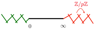
Figure 1. Picture notation for the moduli space of quasimaps $\textsf{QM}^{(p)}_{0,\text{rel}\,\infty}$

4.3. Example

Consider $X=T^{*}\mathbb{P}^{0}$ as the simplest example. The fundamental solution, which is a scalar function in this case, reads

$$\Psi(z,a,q)=\frac{\varphi(\hbar z)}{\varphi(z)}$$

which satisfies the following difference equation

$$\Psi(qz,a,q)=\frac{1-z}{1-\hbar z}\Psi(z,a,q)\,.$$

Thus

$$\Psi(z,a,q)\Psi\left(z^{p},a^{p},q^{p^{2}}\right)^{-1}=\exp\left[\sum_{m=1}^{\infty}\frac{(\hbar^{m}-1)z^{m}}{m(q^{m}-1)}-\frac{(\hbar^{pm}-1)z^{pm}}{pm(q^{pm}-1)}\right]$$

Taking the limit $q\longrightarrow\zeta_{p}$ we get

$$\mathsf{F}(z,\zeta_{p})=\prod_{m,\,p\nmid m}\exp\frac{(\hbar^{m}-1)z^{m}}{m(\zeta_{p}^{m}-1)}\,.$$

5. $p$-Curvature and Frobenius

In this section we discuss reduction of the isospectrality Theorem 4.2 to a field of finite characteristic. First, we recall that over $\mathbb{C}$ the cohomological limit $q$-difference equation gives the quantum differential equation. Second, we consider this limit over $\mathbb{Q}_{p}$ and then reduce it to the finite field $\mathbb{F}_{p}$.

5.1. Quantum Differential Equation as a Limit of (1.1)

It is well known that the quantum differential equation for a Nakajima variety $X$ arises as a limit of $q$-difference equation (1.1). The quantum differential equation for a Nakajima variety $X$ has the form:

(5.1) $$\nabla_{i}\Psi(z)=0,\qquad\nabla_{i}=\kappa\,z_{i}\frac{\partial}{\partial z_{i}}-C_{i}(\mathbold{z},\mathbold{u})$$

where $C_{i}(\mathbold{z},\mathbold{u})$ is the operator of quantum multiplication by the first Chern class $c_{1}(\mathcal{L}_{i})$ in quantum cohomology of $X$. The parameter $\kappa\in\mathbb{C}^{\times}$ denotes the equivariant parameter corresponding to the action of torus $\mathbb{C}^{\times}$ on the source of the stable maps $C\cong\mathbb{P}^{1}$. Together this gives a flat connection $\nabla=(\nabla_{1},\dots,\nabla_{l})$.

The quantum differential equation (5.1) can be obtained from K-theoretic quantum difference equation (1.1) as follows: let $\epsilon$ be a complex parameter with small complex norm, i.e. $|\epsilon|\ll 1$ and assume

(5.2) $$q=1+\kappa\epsilon+O(\epsilon^{2}),\ \ a_{i}=1+\epsilon u_{i}+O(\epsilon^{2})$$

then, the following expansion is well known:

$${\bf M}_{\mathcal{L}_{i}}(\mathbold{z},\mathbold{a},q)=1+\epsilon\,C_{i}(\mathbold{z},\mathbold{u})+O(\epsilon^{2}).$$

Next, let $q^{z_{i}\frac{\partial}{\partial z_{i}}}$ denote the operator acting by shifting the Kähler parameters $z_{i}\mapsto z_{i}q$:

$$q^{z_{i}\frac{\partial}{\partial z_{i}}}f(z_{1},\dots,z_{i},\dots,z_{l})=f(z_{1},\dots,,z_{i}q,\dots z_{l}).$$

Clearly, from (5.2) we have

(5.3) $$q^{z_{i}\frac{\partial}{\partial z_{i}}}=1+\epsilon\kappa\frac{\partial}{\partial z_{i}}+O(\epsilon^{2}).$$

Using the expansions (5.2) and (5.3) we obtain differential equation (5.1) as a first non-trivial term in $\epsilon$ of (1.1). Dividing by $\kappa$ we can rewrite this connection in the form

(5.4) $$\nabla^{L}_{i}=z_{i}\frac{\partial}{\partial z_{i}}-s\,C_{i}(\mathbold{z}),\qquad s=1/\kappa\,.$$

In this formulation, the quantum differential equation is referred to as a pencil in [2024arXiv240100636E, EV2024]. We introduce the superscript $L$ to denote the logarithmic connection. Below, we compare the logarithmic and standard connections modulo $p$. It is worth noting that, in loc. cit., the pencil involved as many parameters, $s_{1},\dots,s_{l}$, as the dimension of the manifold on which it was defined. In contrast, our geometric setup features a single pencil parameter, arising from the torus action on the source curve.

5.2. Reduction to Finite Characteristic

Let $p$ be prime, let $\mathbb{Q}_{p}$ be the field of $p$-adic numbers and $\mathbb{Z}_{p}\subset\mathbb{Q}_{p}$ the the ring of integers. By $\Omega$ we also denote the algebraic closure of $\mathbb{Q}_{p}$ and by $|\cdot|_{p}$ the multiplicative $p$-adic norm normalized so that

$$|p|_{p}=\dfrac{1}{p}$$

The field $\mathbb{Q}_{p}$ does not contain non-trivial $p$-th roots of unity. For this reason, we need to consider an extension $\mathbb{Q}_{p}(\pi)$ where $\pi$ denotes a root of the equation $\pi^{p-1}=-p$. Clearly, the $p$-adic norm of $\pi$ equals:

$$|\pi|_{p}=\dfrac{1}{p^{\frac{1}{p-1}}}.$$

The field $\mathbb{Q}_{p}(\pi)$ contains all $p$-th roots of unity $\zeta_{p}$. It is known that these roots are of the form

$$\zeta_{p}=1+b\pi+O(\pi^{2})\,,\qquad b=0,1,\dots,p-1.$$

In the ring $\mathbb{Z}_{p}[\pi]\subset\mathbb{Q}_{p}(\pi)$ the ideal $(\pi)$ is maximal with the residue field

$$\mathbb{Z}_{p}[\pi]/(\pi)=\mathbb{F}_{p}.$$

Lemma 5.1.

Let $\alpha$ and $\beta$ be two non-commuting operators. Then

$$(1+\pi\alpha+\pi^{2}\beta)^{p}=1+\pi^{p}(\alpha^{p}-\alpha)+O(\pi^{p+1})$$

Proof.

We get

(5.5) $$(1+\pi\alpha+\pi^{2}\beta)^{p} =\sum_{k=0}^{p}\binom{p}{k}(\pi\alpha+\pi^{2}\beta)^{k}=1+p(\pi\alpha+\pi^{2}\beta)+\frac{p(p-1)}{2}(\pi\alpha+\pi^{2}\beta)^{2}$$

$$+\dots+(\pi\alpha+\pi^{2}\beta)^{p}\,.$$

Recall that $p=-\pi^{p-1}$ thus in the lowest order in $\pi$ the following terms remain

(5.6) $$(1+\pi\alpha+\pi^{2}\beta)^{p}=1-\pi^{p}\alpha+\pi^{p}\alpha^{2}+O(\pi^{p+1})\,,$$

where in the second term $-\pi^{p}\alpha=p\pi\alpha$. ∎

5.3. Logarithmic vs. Ordinary Connections

Let $A(z)$ be an $N\times N$ matrix with coefficients in $\mathbb{Q}(z)$. Let $p$ be a prime such that coefficients $A(z)$ have good reduction modulo $p$, i.e. do not have $p$ in the denominators. Clearly any $A(z)\in Mat_{N}(\mathbb{Q}(z))$ has good reduction for all but finitely many $p$.

Let us define the connection $\nabla$ and the logarithmic connection $\nabla^{L}$ as follows.

(5.7) $$\nabla=\dfrac{\partial}{\partial z}+sA(z),\qquad\nabla^{L}=z\dfrac{\partial}{\partial z}+szA(z)\,.$$

They depend on the auxiliary parameter $s$ which appeared in the definition of a pencil.

Lemma 5.2.

The following holds modulo prime $p$

(5.8) $$\left(\nabla^{L}\right)^{p}-\nabla^{L}=z^{p}\nabla^{p}\pmod{p}$$

Proof.

First, let us assume that the connection matrix in (5.7) is trivial $A(z)=0$. Then for a section $f$ we get

$$\left(\nabla^{L}\right)^{p}f(z)=(z\partial)\dots(z\partial)f(z)$$

where one acts with the operators $z\partial=z\frac{\partial}{\partial z}$ on $f$ successively from the right. Let

$$\left(z\partial\right)^{n}f(z)=zf^{\prime}(z)+\sum_{k=2}^{n-1}a_{n,k}z^{k}f^{(k)}(z)+z^{n}f^{(n)}(z)\,.$$

Once can immediately observe the following recursive relation between the coefficients $a_{n,k}$

$$a_{n+1,k}=a_{n,k-1}+k\cdot a_{n,k}\,,$$

which is somewhat reminiscent of the Pascal triangle. This recursive relation is solved by the second Stirling numbers – the number of ways to partition a set of $n$ objects into $k$ non-empty subsets

$$a_{n,k}=\frac{1}{k!}\sum_{j=0}^{k}(-1)^{k-j}\binom{k}{j}j^{n}\,.$$

When $n=p$ is prime by the little Fermat theorem $j^{p}\equiv j$ mod $p$ so

$$a_{p,k}\equiv\frac{1}{k!}\sum_{j=0}^{k}(-1)^{k-j}\binom{k}{j}j\,.$$

for when $j<p$. The latter expression is equal to zero thanks to the following observation for $k>1$

$$0=\frac{d}{da}(1-a)^{k}|_{a=1}=\sum_{j=1}^{k}(-1)^{j}\binom{k}{j}j\,.$$

Thus $a_{p,k}\equiv 0\pmod{p}$ for $1<k<p$ and

(5.9) $$\left(z\partial\right)^{p}f(z)\equiv zf^{\prime}(z)+z^{p}\partial^{p}f(z)\pmod{p}\,.$$

The complete statement of the Lemma for the nontrivial connection $A(z)$ follows after twisting the equation (5.9) with the following operator

(5.10) $$\exp\left[-s\int^{z}A(y)dy\right]\cdot\left(z\partial\right)^{n}\cdot\exp\left[s\int^{z}A(y)dy\right]=\exp\left[-s\int^{z}A(y)dy\right]\cdot\left(\nabla^{L}\right)^{n}\cdot\exp\left[s\int^{z}A(y)dy\right]$$

and similarly on its right hand side. Here we substituted the identity operators between $(z\partial)\cdot 1\cdot(z\partial)$ with the product of the above exponential and its inverse. Then the coefficients in front of the terms containing derivatives of $f$ are the same as $a_{n,k}$ which vanish modulo $p$. ∎

Remark. One can generalize (5.10) by twisting the derivative with the following operator

$$\exp\left[-\sum_{i}s_{i}\int^{z}A_{i}(y)dy\right]\,.$$

This will yield the multi-parameter pencil connection of [2024arXiv240100636E, EV2024].

5.4. Reduction Modulo $\pi$

Given a connection $\nabla$ (5.7) one defines the $p$-curvature as follows

(5.11) $$C_{p}(\nabla)=\nabla^{p}\,,$$

modulo $p$ acting on sections of the bundle in question. Notice that the operator $\partial_{z}^{p}$ acts trivially on functions in characteristic $p$. Furthermore, by the Newton binomial theorem, the coefficients of terms where the derivative acts on the section are proportional to $p$, rendering them trivial modulo $p$. Consequently, the $p$-curvature is purely a matrix operator that involves no derivatives.

Assume that $q\in\mathbb{Q}_{p}(\pi)$ is a $p$-th root of unity, then, without loss of generality, we have

$$q=1+\pi+O(\pi^{2})\,.$$

The $q$-shift operator thus has the following expansion

(5.12) $$q^{z_{i}\frac{\partial}{\partial z_{i}}}=1+\pi z_{i}\frac{\partial}{\partial z_{i}}+O(\pi^{2})$$

Consider quantum difference operator $\mathbf{M}_{\mathcal{L}_{i}}(\mathbold{z},\mathbold{a},q)$ (1.1). Using the above presentation we can write the iterated product (1.11) as

(5.13) $${\bf M}_{\mathcal{L}_{i}\,\zeta_{p}}(\mathbold{z},\mathbold{a},q)=\left(\mathbf{M}_{\mathcal{L}_{i}}(\mathbold{z})q^{z_{i}\frac{\partial}{\partial z_{i}}}\right)^{p}\,.$$

From (5.12) in the order up to $\pi^{2}$ one gets

$$\mathbf{M}_{\mathcal{L}_{i}}(\mathbold{z},\mathbold{a},q)q^{z_{i}\frac{\partial}{\partial z_{i}}}=(1+\pi s\,z_{i}A_{i}(\mathbold{z})+O(\pi^{2}))\left(1+\pi z_{i}\frac{\partial}{\partial z_{i}}+O(\pi^{2})\right)$$

where we redefined Chern classes in (5.4) as $C_{i}(\mathbold{z})=z_{i}A_{i}(\mathbold{z})$. This expression simplifies to the following

$$\mathbf{M}_{\mathcal{L}_{i}}(\mathbold{z},\mathbold{a},q)q^{z_{i}\frac{\partial}{\partial z_{i}}}=1+\pi\nabla_{i}^{L}(z)+O(\pi^{2})\,.$$

Next, thanks to Lemma 5.1 for $\alpha=\nabla_{i}^{L}$, we get

$$\left(\mathbf{M}_{\mathcal{L}_{i}}(\mathbold{z},\mathbold{a},q)q^{z_{i}\frac{\partial}{\partial z_{i}}}\right)^{p}=1+\pi^{p}\left(\left(\nabla_{i}^{L}\right)^{p}-\nabla_{i}^{L}\right)+O(\pi^{p+1})\,.$$

Finally, by Lemma 5.2 and (5.13) we obtain

(5.14) $$\frac{{\bf M}_{\mathcal{L}_{i}\,\zeta_{p}}(\mathbold{z},\mathbold{a},q)-1}{\pi^{p}}\equiv\nabla_{i}^{p}\pmod{\pi}$$

which is precisely the $p$-curvature $C_{p}(\nabla_{i})$ of the connection $\nabla_{i}$ (5.11). This demonstrates that the iterated product of the quantum difference operators $\mathbf{M}_{\mathcal{L}_{i}\,\zeta_{p}}(\mathbold{z},\mathbold{a},q)$ reduces to the $p$-curvature modulo $\pi\in\mathbb{Q}_{p}(\pi)$.

5.5. Matching

Now let us consider the quantum difference operator after the Frobenius action on its arguments $\mathbf{M}_{\mathcal{L}_{i}}(\mathbold{z}^{p},a^{p},q^{p})$. From the above it follows that

$$(1+\pi s)^{p}=1+\pi^{p}(s^{p}-s)+O(\pi^{p+1})$$

This means that the operator will have the following expansion in $\pi$

$$\mathbf{M}_{\mathcal{L}_{i}}(\mathbold{z}^{p},\mathbold{a}^{p},q^{p})=1+z_{i}^{p}A_{i}(\mathbold{z}^{p})\pi^{p}(s^{p}-p)+O(\pi^{p+1})$$

In other words,

(5.15) $$\frac{\mathbf{M}_{\mathcal{L}_{i}}(\mathbold{z}^{p},\mathbold{a}^{p},q^{p})-1}{\pi^{p}}\equiv(s^{p}-s)z_{i}^{p}A_{i}(\mathbold{z}^{p})\pmod{\pi}\,.$$

By comparing (5.14) with (5.15) we obtain a theorem by Etingof and Varchenko from the isospectrality of ${\bf M}_{\mathcal{L}_{i}\,\zeta_{p}}(\mathbold{z},\mathbold{a},q)$ and $\mathbf{M}_{\mathcal{L}_{i}}(\mathbold{z}^{p},\mathbold{a}^{p},q^{p})$.

Theorem 5.3 ([EV2024]).

The spectra of the periodic pencil $(s^{p}-s)A\circ F_{p}$, where $F_{p}$ is the Frobenius map, and the $p$-curvature $C_{p}(\nabla_{i})$ are isomorphic modulo $p$.

References

• \ProcessBibTeXEntry \ProcessBibTeXEntry \ProcessBibTeXEntry \ProcessBibTeXEntry \ProcessBibTeXEntry \ProcessBibTeXEntry \ProcessBibTeXEntry \ProcessBibTeXEntry \ProcessBibTeXEntry \ProcessBibTeXEntry \ProcessBibTeXEntry \ProcessBibTeXEntry \ProcessBibTeXEntry \ProcessBibTeXEntry \ProcessBibTeXEntry \ProcessBibTeXEntry \ProcessBibTeXEntry \ProcessBibTeXEntry \ProcessBibTeXEntry