Critical Measures and the Zakharov-Shabat spectrum

Abstract

We consider the family of (poly)continua $\mathcal{K}$ in the upper half-plane ${{\mathbb{H}}}$ that contain a preassigned finite anchor set $E$. For a given harmonic external field we define a Dirichlet energy functional $\mathcal{I}(\mathcal{K})$ and show that within each “connectivity class” of the family, there exists a minimizing compact $\mathcal{K}^{*}$ consisting of critical trajectories of a quadratic differential. In many cases this quadratic differential coincides with the square of the real normalized quasimomentum differential ${\mathrm{d}}\mathbf{p}$ associated with the finite gap solutions of the focusing Nonlinear Schrödinger equation (fNLS) defined by a hyperelliptic Riemann surface $\mathfrak{R}$ branched at the points $E\cup\bar{E}$.

An fNLS soliton condensate is defined by a compact $\mathcal{K}\subset{{\mathbb{H}}}$ (its spectral support) whereas the average intensity of the condensate is proportional to $\mathcal{I}(\mathcal{K})$ with external field given by $\mathrm{Im}\,z$. The motivation for this work lies in the problem of soliton condensate of least average intensity such that $E$ belongs to the poly-continuum $\mathcal{K}$. We prove that spectral support $\mathcal{K}^{*}$ provides the fNLS soliton condensate of the least average intensity within a given “connectivity class”.

1 Introduction

A continuum is a compact, connected set with at least two distinct points and a poly-continuum is a finite union thereof. Let $E\subset{\mathbb{C}}$ be a finite set of points, called “anchors”, and $\mathcal{K}\subset{\mathbb{C}}$ be a continuum containing $E$. The well known Chebotarev’s continuum problem is to find such a continuum $\mathcal{K}$ of minimal logarithmic capacity ${\rm cap}(\mathcal{K})$. We recall that ${\rm cap}(\mathcal{K}):={\rm e}^{-\mathcal{E}(\mathcal{K})}$, where

$$\mathcal{E}(\mathcal{K}):=\inf\left\{\iint\ln\frac{1}{|z-w|}{\mathrm{d}}\mu(z)d\mu(w)\right\}$$ (1.1)

taken among all positive unit Borel measures supported within $\mathcal{K}$. Thus the problem can be stated as that of finding the maximizer of the logarithmic energy $\mathcal{E}(\mathcal{K})$ among all the continua containing $E$. This problem was solved around 1930 in [10], [21, 22], see for example [23], where the minimizing ${\rm cap}(\mathcal{K})$ compact $\mathcal{K}$ was represented as the set of critical trajectories of a certain quadratic differential on the hyperelliptic Riemann surface defined by $E$.

The main problem considered in this paper is of a similar nature but with a different energy functional, a different class of measures involved and a bit different overall setting. Namely, the set $E$ belongs to the upper half plane ${{\mathbb{H}}}=\{z\in{\mathbb{C}}:\ \mathrm{Im}\,(z)>0\}$ and instead of the free logarithmic energy (1.1) we consider the Green energy

$$\mathfrak{J}(\mathcal{K}):=\inf\left\{\iint\ln\frac{|z-\bar{w}|}{|z-w|}{\mathrm{d}}\mu(z)d\mu(w)-2\int\mathrm{Im}\,zd\mu(z)\right\}$$ (1.2)

with infimum taken over all positive (but of arbitrary total mass) Borel mausures supported on $\mathcal{K}\subset\overline{{{\mathbb{H}}}}$. Here $-2\mathrm{Im}\,z$ represents the external field, so (1.2) represents the weighted Green energy $\mathfrak{J}(\mathcal{K})$ of the minimizing measure on $\mathcal{K}$: observe that since $\mathcal{K}\subset\overline{{{\mathbb{H}}}}$, we have that $\mathfrak{J}(\mathcal{K})<0$. More generally, we will be looking at the extremal problem not only in the class of continua $\mathcal{K}\supset E$, but also in the classes of poly-continua $\mathcal{K}\supset E$, where each connected component of $\mathcal{K}$ contains at least two points of $E$ or connects a point of $E$ with ${\mathbb{R}}$. To the best of our knowledge, this type of extremal problems were not considered in the literature. The most relevant statement we could find is Theorem 6.1 from [27], stated without full proof, where $\mathfrak{J}$ is a Green energy functional on positive Borel measures of total mass one. To give an immediate visual example, we show in Fig. 6 the continua of minimal weighted Green energy (1.2) with the property that $\mathcal{K}\supset E$ and $\mathcal{K}\cap{\mathbb{R}}\neq\emptyset$.

The interest in this extremal (max-min) problem originates from the problem of finding a compact spectral support, $\Gamma^{+}$, of the fNLS soliton condensate of minimal average intensity, given a fixed finite “anchor” set $E\in\Gamma^{+}$. Similar problem can be formulated about the Zakharov–Shabat spectrum of finite gap fNLS solutions defined by spectral hyperelliptic Riemann surface branched at $\hat{E}=E\cup\bar{E}$. To better frame our results we provide a concise description of the fNLS finite gap solutions and fNLS soliton condensates hereafter.

1.1 Focusing NLS and extremal problems

Consider the focusing Nonlinear Schrödinger Equation (fNLS)

$$i\partial_{t}\psi=-\partial_{x}^{2}\psi-2|\psi|^{2}\psi.$$ (1.3)

If $\psi=\psi(x,t)\in L^{2}_{loc}$ is a bounded function of $x$, but not necessarily vanishing at $\pm\infty$, one can consider the “average intensity” of $\psi$, namely the limit

$$\mathcal{I}=\lim_{L\to\infty}\frac{1}{2L}\int_{-L}^{L}|\psi(x,t)|^{2}{\mathrm{d}}x.$$ (1.4)

Important classes of solutions to (1.3) are given by the “finite gap solutions” [1], which are quasi-periodic (in $x$ and in $t$) solutions of (1.3) constructed in the seventies [12]. These solutions involve a hyperelliptic Riemann surface $\mathfrak{R}$ of genus $g$ represented as a double cover of the spectral $z$–plane (a sort of “Fourier” variable associated to the solution) branched at $2g+2$ points coming in $g+1$ conjugate pairs. The average intensity $\mathcal{I}$ is conserved in time if $\psi(x,t)$ satisfies (1.3) ([1], [7]).

Recent literature devotes a considerable effort towards the mathematical study of “soliton gases”; the term is used to refer to a couple of approaches that all involve some limiting procedure taken either on special families of $N$-soliton solutions to (1.3) with $N\to\infty$ or on certain meromorphic differentials on $X$, related with the finite gap solutions of (1.3), with $g\to\infty$. In the first case, ideally, one would want to consider some statistical ensembles of infinitely many solitons but in practice, thus far, the state of the art is rather in the direction of choosing a specific $N$-soliton solution, taking the limit $N\to\infty$, and then addressing questions about the behaviour of the limiting solution ([2, 8]). In the second case, while $g\to\infty$, the spectral bands (the branchcuts of $X$) are scaled down at a certain rate and in such a way that they fill densely a certain one or two dimensional compact $\Gamma^{+}\subset{{\mathbb{H}}}$, [6], [32]. This limiting procedure is known as thermodynamic limit. The remarkable difference with the previous approach is that here we are primarily interested in some “macroscopic” observable quantities, such as, for example, the effective speed of an element of the soliton gas or the average intensity (of the gas), rather than in reconstruction of particular realizations of the gas, provided that such limiting realization exist. Ideally one would want to calculate large $g$ limits of some statistical characteristics of the finite gap solutions on $X$, such as, for example, the probability distribution of $|\psi|^{2}$, the moments of this distribution, etc. One of the most important macroscopic property of soliton gases with physical relevance is the limiting average intensity $\mathcal{I}$, (1.4). Well known results allow to express $\mathcal{I}$ for any finite gap solution and, thus, a suitable description can be obtained in the large genus (thermodynamic) limit. The main thrust in the present work is to find the compact accumulation (spectral support) set $\Gamma^{+}\subset{{\mathbb{H}}}$ of the growing number of small bands (with $E\subset\Gamma^{+}$) that minimizes the average intensity $\mathcal{I}$, given by (1.4), for the special type of the fNLS soliton gases, called soliton condensates, see Section 1.3 for more details.

As it will be shown below, the average intensity $\mathcal{I}$ of fNLS soliton condensate is proportional to $-\mathfrak{J}(\mathcal{K})$(1.2), i.e., to (minus) the Green energy of the compact $\Gamma^{+}$. We will also show that the average intensity $\mathcal{I}$ is proportional to the Dirichlet energy (in $\Omega={{\mathbb{H}}}\setminus\Gamma^{+}$) of the Green potential

$$G(z)=\int_{\Gamma^{+}}\ln\frac{|z-\bar{w}|}{|z-w|}{\mathrm{d}}\mu(w)$$ (1.5)

of the equilibrium measure $\mu(z)$, which we sometimes refer to as the Diriclet energy of the compact $\Gamma^{+}\subset{{\mathbb{H}}}$. With a slight abuse of notations, we often use the notation $\mathcal{I}=\mathcal{I}(\mathcal{K})$ to denote the Diriclet energy of the compact $\mathcal{K}\subset{{\mathbb{H}}}$. We now describe the setting of the extremal problems studied in this paper.

1.2 Description of the problems

Let a compact $\Gamma^{+}\subset{{\mathbb{H}}}$ be a collection of piece-wise smooth curves, which can transversally intersect each other and ${\mathbb{R}}$. Denote by $E=\{e_{1},\dots,e_{N}\}$ the set of endpoints of $\Gamma^{+}$ in ${{\mathbb{H}}}$ or anchors. It was shown in [17], see also Subsection 1.3, that, given $\Gamma^{+}$, the (fNLS) soliton condensate (with $\sigma\equiv 0$ in the notation of loc. cit.) maximizes the average intensity $\mathcal{I}$ (the Dirichlet energy) among all the soliton gases with spectral support $\Gamma^{+}$. Then a natural question is what contour $\Gamma_{+}$ minimizes $\mathcal{I}=\mathcal{I}(\Gamma^{+})$ for given anchor set $E$?.

Let $\mathcal{R}_{N}$ denote a hyperelliptic Riemann surface (RS) of genus $N-1$ with branchcuts ending at $\hat{E}=E\cup\bar{E}$ and let $d\mathbf{p}_{N}$ be a real normalized quasimomentum differential on $\mathcal{R}_{N}$. Note that $d\mathbf{p}_{N}$ is uniquely defined on $\mathfrak{R}_{N}$ ([29, 11]) and is Schwarz symmetrical. The naïve (but in general wrong, as it turns out) idea is that the set minimizing the average intensity should consist of critical trajectories of the quadratic differential ${\mathrm{d}}\mathbf{p}_{N}^{2}$, namely, of the zero level curves of $\mathrm{Im}\,\mathbf{p}_{N}(z)$ in ${{\mathbb{H}}}$ emanating from the points in $E$ (we assume $\mathrm{Im}\,\mathbf{p}_{N}(x)=0$ for any $x\in{\mathbb{R}}$): this set represents the spectrum of the first Lax equation for the NLS, known as Zakharov-Shabat (ZS) equation (Section 2) and, therefore, we will call it Zakharov–Shabat spectrum of the quasimomentum ${\mathrm{d}}\mathbf{p}_{N}$. With a slight abuse of notation, we will also call $\Gamma^{+}$ the Zakharov–Shabat spectrum of the quadratic differential ${\mathrm{d}}\mathbf{p}^{2}_{N}$.

We found that in certain cases the ZS spectrum of ${\mathrm{d}}\mathbf{p}_{N}$ is indeed the minimizer of $\mathcal{I}$. For example, this is always the case when $N\leq 2$. But for $N=3$, there are geometrical configurations of the anchor set $E$ where the minimizer $\mathcal{I}(\Gamma^{+})$ is not the Zakharov–Shabat spectrum of ${\mathrm{d}}\mathbf{p}_{N}$, see caption to Fig. 1

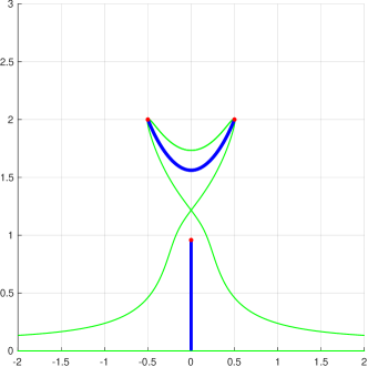
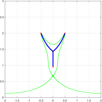
Figure 1: The anchor sets (red dots) and the Dirichlet energies of the sets marked in blue are the same in both figures, approximately $2.7299$. Note that the two set have “incommensurable” connectivity. The set on the left represents the Zakharov–Shabat spectrum of ${\mathrm{d}}\mathbf{p}^{2}_{N}$. If the anchor point on the imaginary axis is moved slightly down, the Zakharov–Shabat spectrum is the one of minimal energy, viceversa if we move the anchor upwards, the other wins.

It is more convenient to describe our results in terms of quadratic differentials. The quasimomentum differential has the form

$${\mathrm{d}}\mathbf{p}_{N}=\frac{P_{N}(z){\mathrm{d}}z}{\prod_{j=1}^{N}\sqrt{(z-e_{j})(z-\bar{e}_{j})}},$$ (1.6)

where $P_{N}$ is a monic polynomial of degree $N$ whose coefficients are uniquely defined by the condition of being residue-less and with purely real periods. The corresponding quadratic differential has the form ${\mathrm{d}}\mathbf{p}_{N}^{2}=Q(z){\mathrm{d}}z^{2}$, where the rational function $Q(z)=\frac{P_{N}^{2}(z)}{R^{2}(z)}$ has, generically, only zeros of even multiplicity and simple poles at $e_{j},\bar{e}_{j}$. Here $R(z)$ denotes the denominator of (1.6), satisfying $R(z)\sim z^{N}$ as $z\to\infty$. We generalize these by replacing $P_{N}^{2}$ in the numerator of $Q$ with a monic polynomial $P_{2N}$ of the same degree $2N$ (not necessarily a complete square) that we call quasimomentum type quadratic differentials. More precisely we define quasimomentum type quadratic differentials as rational, Schwarz symmetric Boutroux quadratic differentials

$$Q{\mathrm{d}}z^{2}=\frac{P_{2N}(z)}{\prod_{j=1}^{N}(z-e_{j})(z-\bar{e}_{j})}{\mathrm{d}}z^{2},\quad\text{where}\quad\mathcal{P}_{2N}=z^{2N}-2\left(\sum_{j=1}^{N}\mathrm{Re}\,e_{j}\right)z^{2N-1}+\dots\,.$$ (1.7)

The latter condition implies that $\sqrt{Q}{\mathrm{d}}z$ is residue-less, whereas “Boutroux” means that $\sqrt{Q}{\mathrm{d}}z$ is real-normalized on the Riemann surface defined by the equation $y^{2}=Q(z)$. In general, $P_{2N}$ can have $\ell$, $0\leq\ell\leq N-1$ odd order roots $a_{1},\dots,a_{\ell}$ (counted with multiplicities) in ${{\mathbb{H}}}$ and their complex conjugates in the lower half plane ${{\mathbb{H}}}-$. If all $a_{k}$, $1\leq k\leq\ell$, are distinct and are not in $E$, then $\sqrt{Q}{\mathrm{d}}z$ is the (unique) real normalized quasimomentum differential defined on the Riemann surface $\mathfrak{R}_{L}$, $L=N+\ell$, with $L$ branchpoints $e_{1},\dots,e_{N},a_{1},\dots,a_{\ell}$ on ${{\mathbb{H}}}$ and their complex conjugates. In degenerate cases, some odd order roots $a_{k}$ of $P_{2N}$ may coincide with each other or with points $e_{j}$ from $E$.

Our main results can be encapsulated in the statement:

the minimizing set of the Green energy (1.2) is the zero level set of $\mathrm{Im}\,\int_{0}^{z}\sqrt{Q}(\zeta){\mathrm{d}}\zeta$ in ${{\mathbb{H}}}$ for some quasimomentum type quadratic differential.

A more detailed statement requires us to classify families, over which we mininimize $\mathcal{I}$, by their “connectivity” . Given a finite anchor set $E\subset{{\mathbb{H}}}$ we define the family ${\mathbb{K}}_{E}$ consisting of all poly-continua $\mathcal{K}$ where each component contains at least two different anchor points or connects an anchor $e\in E$ with a point in ${\mathbb{R}}$. We denote the components as $\mathcal{K}=\sqcup_{\ell=0}^{k}\mathcal{K}_{\ell}$, where $\mathcal{K}_{\ell}$, $\ell=1,\dots,k,$ are the connected components of $\mathcal{K}$ not meeting ${\mathbb{R}}$, and the notation $\mathcal{K}_{0}$ is reserved for the component that meets ${\mathbb{R}}$, if any is present. This partition of a poly-continuum $\mathcal{K}\in{\mathbb{K}}_{E}$ allow us to define the connectivity of $\mathcal{K}$ as an $(N+1)$ by $(N+1)$ symmetric matrix $M=M(\mathcal{K})$ (connectivity matrix) where $M_{i,j}=1$ means that $e_{i},e_{j}$ belong to the same component $\mathcal{K}_{\ell}$, $0\leq\ell\leq k$ $i,j\leq N$, and $M_{i,0}=1$ means that $e_{i}$ is connected with ${\mathbb{R}}$, i.e, $e_{i}\in\mathcal{K}_{0}$; the remaining entries of $M$ are zeros. We say that compacts $\mathcal{K}^{(1)},\mathcal{K}^{(2)}\in{\mathbb{K}}_{E}$ have the same connectivity if $M(\mathcal{K}^{(1)})=M(K^{(2)})$. We say that $\mathcal{K}^{(2)}$ has a larger connectivity than $\mathcal{K}^{(1)}$, if $M(\mathcal{K}^{(2)})_{i,j}\geq M(\mathcal{K}^{(1)})_{i,j}$, $i,j=0,2\dots,N$. It is clear that there are finitely many different connectivities within the class ${\mathbb{K}}_{E}$. For a given anchor set $E$ we define subclasses ${\mathbb{K}}_{E,M}\subset{\mathbb{K}}_{E}$, where each subclass consists of poly-continua with larger connectivity than the one of the matrix $M$. We can now formulate our main result.

Theorem 1.1

(a) For every connectivity $M$ the class ${\mathbb{K}}_{E,M}$ contains a minimizer $\mathfrak{F}$ of the Dirichlet energy $\mathcal{I}$.
(b) This minimizer consists of all the zero level curves of $\mathrm{Im}\,\int_{0}^{z}\sqrt{Q}(\zeta){\mathrm{d}}\zeta=0$ restricted to ${{\mathbb{H}}}$, where the quasimomentum type quadratic differential $Q{\mathrm{d}}z^{2}$ is as in (1.7); this set is called the Zakharov–Shabat spectrum of $Q{\mathrm{d}}z^{2}$.
(c) For any quasimomentum type quadratic differential $Q{\mathrm{d}}z^{2}$, its Zakharov–Shabat spectrum $\mathfrak{F}$ is the unique minimizer within ${\mathbb{K}}_{E,M}$, where $M$ is the connectivity matrix of $\mathfrak{F}$.

Theorem 1.1 provides a solution to the problem that in some sense is similar to the Chebotarev’s continuum problem with the following distinctions: a) the logarithmic energy $\mathcal{E}$ is replaced by the Dirichlet energy $\mathcal{I}$ (weighted Green energy $\mathfrak{J}$ with the opposite sign); b) there is no restriction for the total mass of positive Borel measures defining $\mathcal{I}(\mathcal{K})$ for compacts $\mathcal{K}\subset{{\mathbb{H}}}$; c) instead of minimizing among the continua, containing a given set $E$, we minimize among the poly-continua (containing $E$) of a prescribed connectivity defined by matrix $M$.

We also prove that the Zakharov–Shabat spectrum of ${\mathrm{d}}\mathbf{p}_{N}$ minimizes $\mathcal{I}(\Gamma^{+})$ among all possible (Schwarz symmetric) branchcuts of the Riemann surface $\mathfrak{R}_{N}$.

The key technical tool in the proof of Theorem 1.1 is Jenkins’ interception property, a generalization of an idea of Jenkins’ formulated in [14], see Section 4. The proof of this property is based on the “length-area” method [10]. We made some extension in the original statement of this method ([13]), so that it allows us to compare Dirichlet energies of different $\mathcal{K}\in{\mathbb{K}}_{E}$, provided that certain “interception conditions”, see Definition 4.1, are met. Then part b) of Theorem 1.1 follows as a consequence. In order to prove the statement of part a) of Theorem 1.1, we use the fact that each class ${\mathbb{K}}_{E,M}$ is closed in Hausdorff metric and then we prove that the energy functional $\mathcal{I}(\mathcal{K})$ is continuous in that metric and, thus, there exists a minimizer, see Sections 5,6. Part of this proof consist in establishing that there exists a minimizing sequence of poly-continua in ${\mathbb{K}}_{E,M}$ that is uniformly bounded in ${{\mathbb{H}}}$, see Section 6, where Jenkins’ property is utilized for this proof. The remaining part c) of Theorem 1.1 is proved by using Schiffer variation approach, see Section 7.

In the following Section 1.3 we provide some background information on soliton gases for integrable equations. Then, in Section 2, we discuss the Zakharov–Shabat spectra of finite gap fNLS solutions defined by the Riemann surface $\mathfrak{R}_{N}$ with its quasimomentum differential ${\mathrm{d}}\mathbf{p}_{N}$. We also introduce quadratic differentials and define extensions of $\mathfrak{R}_{N}$ there. In the following Section 3 we introduce generalized quasimomentum associated with a compact $\mathcal{K}\subset{{\mathbb{H}}}$ and establish their main properties, required for Section 4 to prove Jenkins’ interception property.

Electrostatic interpretation.

Let us consider the following two–dimensional electrostatic interpretation of the Dirichlet problem for $\mathrm{Im}\,\mathcal{P}(z;\mathcal{K})$ (see Section 3 below): we can imagine that a poly-continuum $\mathcal{K}=\cup_{l=0}^{k}\mathcal{K}_{l}$, see above, is a conductor made of metal with (shielded) connection of each $\mathcal{K}_{l}$, $l\geq 1$, to the ground represented by ${\mathbb{R}}$. Namely, we imagine that each $\mathcal{K}_{l}$, $l\geq 1$, is “floating in the sky” and that there is a shielded wire connecting it to the ground, whereas $\mathcal{K}_{0}$, if not empty, consists of grounded conductor(s).

Suppose that we have very high charged clouds (ideally placed at $i\infty$) generating a constant vertical electric field and hence electrostatic potential $\mathrm{Im}\,(z)$; then the conductors $\mathcal{K}$ will distribute charge (of which there is an infinite reservoir via the ground connection) so as to ground themselves at zero potential. The resulting electrostatic potential is precisely $\mathrm{Im}\,\mathcal{P}(z;\mathcal{K})$. Assume further that the conductors $\mathcal{K}_{l}$, $l=0,\dots,k$, can be elastically deformed (with no loss of energy). The restriction is that such deformations should have fixed points from the finite set $E$ assigned to each conductor (according to the connectivity matrix $M$, where $\mathcal{K}\in{\mathbb{K}}_{E,M}$). Then the problem is to find the shape of $\mathcal{K}$ minimizing the electrostatic energy of $\mathcal{K}$.

1.3 Soliton condensates for integrable equations and other applications

The idea of soliton gas for Korteweg de Vries (KdV) equation goes back to 1971 paper [36] of V. Zakharov, where he calculated the effective velocity of a trial soliton propagating on a multi-soliton background. This background modifies the average speed of the (free) trial soliton because of its repeated interactions with the background solitons, each of which can be regarded as an instanteneous shift of the center (aka as phase shift) of the trial soliton. In the modern language, the setting of [36] corresponds to a diluted KdV soliton gas. In order to study a dense KdV soliton gas, a different approach was suggested by G. El in [4]. This approach is based on styding the finite gap solutions for the KdV, defined by some hyperelliptic Riemann surface $\mathfrak{R}$, where the number $N$ of the bands (branchcuts of $X$) is growing but the size of the (bounded) bands simultaneously go to zero at a certain exponential (in $N$) rate. Each individual decaying band correspond to a soliton in this limit, but the key thing is the right scaling of the decaying bands, which could be found in an earlier work [34] of S. Venakides. Such limit is called thermodynamic limit. One of the main results of [4] are the so called Nonlinear Dispersion Relations (NDR), which define the continualized limits $u(z)$, $v(z)$ of scaled wavenumbers and of scaled frequences respectively of the finite gap KdV solutions in the thermodynamic limit. In spectral theory of soliton gases, $u(z)$ is called the density of states (DOS) and $v(z)$ - the density of fluxes (DOF).

We note that the spectral problem for the KdV is self adjoint so that all the bands of $X$ are on ${\mathbb{R}}$. Deriving the NDR for a non self adjoint problem, such as, for example, Zakharov-Shabat problem for the fNLS, was achieved in [6]. We refer to [6] for details of this derivation. Since the bands of $X$ are now in ${\mathbb{C}}$ (due to Schwarz symmetry, we could restrict our attention to the upper half plane ${{\mathbb{H}}}$ only), the (general) NDR for fNLS soliton gases are complex. For example, the general first NDR for the fNLS soliton gas with a one dimensional accumulation set $\Gamma^{+}\subset{{\mathbb{H}}}$ is

$$i\int_{\Gamma^{+}}\left[\ln\frac{\bar{w}-z}{w-z}+i\pi\chi_{z}(w)\right]u(w)|dw|+i\sigma(z)u(z)=z+\tilde{u}(z)$$ (1.8)

where: $u,\tilde{u}$ are the solitonic and the carrier densities of states (DOS) respectively; $\chi_{z}(w)$ is the indicator function of the (oriented) arc of $\Gamma^{+}$ starting at the beginning of $\Gamma^{+}$ and ending at $z\in\Gamma^{+}$, and; $\sigma\in C(\Gamma^{+})$ is nonnegative on $\Gamma^{+}$. The accumulation set $\Gamma^{+}$ is also called a spectral support set for the corresponding soliton gas. Very often, the imaginary part of (1.8):

$$\int_{\Gamma^{+}}\ln\left|\frac{\bar{w}-z}{w-z}\right|u(w)|dw|+\sigma(z)u(z)=\mathrm{Im}\,z,$$ (1.9)

defining the solitonic DOS $u(z)$ is called the first NDR in literature ([6], [5]). The general second NDR for the fNLS soliton gas with a one dimensional $\Gamma^{+}\subset{{\mathbb{H}}}$ has the form

$$i\int_{\Gamma^{+}}\left[\ln\frac{\bar{w}-z}{w-z}+i\pi\chi_{z}(w)\right]v(w)|dw|+i\sigma(z)v(z)=-2z^{2}+\tilde{v}(z),$$ (1.10)

where: $v,\tilde{v}$ are the solitonic and the carrier densities of fluxes (DOF) respectively.

Existence and uniqueness of solution $u(z)$ to the first NDR (1.9) with a compact $\Gamma^{+}\subset{{\mathbb{H}}}$ was established [17], subject to some mild restrictions on $\Gamma^{+}$ and $\sigma(z)$. The idea of the proof was to minimize some quadratic energy functional $J_{\sigma}$ among all non negative Borel measures. In the special case $\sigma\equiv 0$ on $\Gamma^{+}$ the energy $J_{0}$ is the Green energy of $\Gamma^{+}\subset{{\mathbb{H}}}$ with the external field $-2\mathrm{Im}\,z$, see [28], Chapter 2. It was also observed ([17]) that $-J_{0}$ coincides with the averege intensity $\mathcal{I}$ of a soliton gas, defined ([32]) as

$$\mathcal{I}=2\int_{\Gamma^{+}}\mathrm{Im}\,(z)\,u(z)d\lambda(z),$$ (1.11)

where $d\lambda$ is a reference measure on $\Gamma^{+}$, such as the arclength or the area.

To have another look on the NDR (1.8), (1.10), we remind that the wavenumbers and frequences of finite gap solutions are represented by periods of quasimomentum ${\mathrm{d}}p_{g}$ and quasienergy ${\mathrm{d}}q_{g}$ meromorphic differentials on $X$ that are normalized in such a way that all their periods are real (real normalized or Boutroux differentials). This normalization uniquely defines ${\mathrm{d}}p_{g},{\mathrm{d}}q_{g}$ (their principlal parts at singular points are fixed). If $A$ cycles are properly oriented small loops around the shrinking bands of $X$, then the $A$ and $B$ periods of ${\mathrm{d}}p_{g}$ are called the solitonic and the carrier wavenumbers of the corresponding finite gap solutions, see [6]. Then the general first NDR (1.8) can be viewed as the thermodynamic limit of the Riemann Bilinear relations between ${\mathrm{d}}p_{g}$ and the normalized holomorphic differentials of $X$, see [33], [16]. Similarly, one can obtain (1.10) from ${\mathrm{d}}q_{g}$. One can also observe that the kernel of the integral operator in (1.8)-(1.10) was obtained as the thermodynamic limit of the Riemann Period matrix of $X=X_{g}$ with $g\to\infty$, where the centers of the corresponding bands of $X_{g}$ approach the values of $w,z\in\Gamma^{+}$ respectively ([32]).

We point out that the fNLS soliton gas with $\sigma\equiv 0$ on $\Gamma^{+}$ defines a special class of soliton gases known as soliton condensates. The maximizing property of condensates was established in [17]. Namely, it was shown there that if a compact $\Gamma^{+}\subset{{\mathbb{H}}}$ is fixed but $\sigma(z)\geq 0$ is allowed to vary, then the condensate $\sigma\equiv 0$ provides the maximum average intensity $\mathcal{I}$ (among all soliton gases with spectral support $\Gamma^{+}$). That observation naturally led to the following question that triggered the work on this paper. Let a compact $\Gamma^{+}\subset{{\mathbb{H}}}$ be a finite collection of piece-wise smooth contours with the fixed endpoints comprising the set $E\subset{{\mathbb{H}}}$. For a given $E$, find $\Gamma^{+}\subset{{\mathbb{H}}}$ that maximizes the Green energy of the soliton condensate defined by $\Gamma^{+}\subset{{\mathbb{H}}}$ with the external field $-2\mathrm{Im}\,z$. Equivalently, one can ask of $\Gamma^{+}\subset{{\mathbb{H}}}$ that minimizes the averege intensity $\mathcal{I}=\mathcal{I}(\Gamma^{+})$) of the fNLS soliton condensate, defined by $\Gamma^{+}$. As it was discussed above, this problem can be considered as some generalized version of the Chebotarev’s continuum problem.

Acknowledgements.

The authors would like to thank the Isaac Newton Institute for Mathematical Sciences, Cambridge, UK, and Northumbria University, Newcastle, UK, for support and hospitality during the satelite programme “Emergent phenomena in nonlinear dispersive waves”, where work on this paper was undertaken. AT was supported by a Simons fellowship for his visit. The authors also gratefully thank Evguenii Rakhmanov and Arno Kuijlaars for helpful discussions. The work of MB was supported in part by the Natural Sciences and Engineering Research Council of Canada (NSERC) grant RGPIN-2023-04747. The work of AT was supported in part by the NSF Grants DMS-2009647, DMS-2407080 and by Simons Foundation award.

2 Zakharov–Shabat differentials and spectra

The Lax pair associated with the Nonlinear Schrödinger equation (1.3) consists of the pair of ODEs

$$i\partial_{x}\Psi(x,t;z)=U(x,t;z)\Psi(x,t;z),\qquad i\partial_{t}\Psi(x,t;z)=V(x,t;z)\Psi(x,t;z),$$ (2.1)

$$U(x,t;z):=\begin{bmatrix}z&{\psi(x,t)}\\ \overline{\psi(x,t)}&-z\end{bmatrix},\qquad V(x,t;z):=2zU(x,t;z)+\begin{bmatrix}-|\psi|^{2}&-i\psi_{x}\\ -i\overline{\psi_{x}}&|\psi|^{2}\end{bmatrix}$$ (2.2)

for the matrix–valued function $\Psi(x,t;z)$. Here $\psi(x,t)$ is a complex–valued function in a suitable class, depending on the problem considered. The compatibility of these two equations requires that $\psi(x,t)$ satisfies (1.3). The $t$–dependence of $\psi$ is not important in our discussion.

The Zakharov–Shabat spectral problem associated with the first equation (2.1), called “Zakharov–Shabat equation”, is the collection of all values $z\in{\mathbb{C}}$ for which the fundamental solution of this equation remains bounded for $x\in{\mathbb{R}}$. If $\psi(x,0)$ is a finite gap solution [1] then $\Psi(x,0;z)$ can be written explicitly in terms of Riemann Theta functions associated to a hyperelliptic Riemann surface $\mathfrak{R}_{L}$ of finite genus $L-1$ branched at $2L$ points $\{b_{1},\dots b_{L},\overline{b}_{1},\dots,\overline{b}_{L}\},\ b_{j}\in{{\mathbb{H}}}\setminus{\mathbb{R}}$. The general structure of the formula (see [12]) is

$$\Psi(x,t;z)=W_{L}(z;x,t){\rm e}^{i{(x\mathbf{p}(z)+t\mathbf{q}(z))}\sigma_{3}},\quad$$ (2.3)

where the only relevant fact we need to recall is that the matrix $W_{L}$ remains bounded in $x\in{\mathbb{R}}$ for all fixed $z\in{\mathbb{C}}$ (and also for all fixed times $t\in{\mathbb{R}}$). As a matter of fact $W_{L}$ is bounded also in $t\in{\mathbb{R}}$, but this fact will not be relevant for this paper. The function $\mathbf{p}(z)$ from (2.3) is precisely the real–normalized quasimomentum integral, that is, the anti-derivative of the unique differential of the second kind ${\mathrm{d}}\mathbf{p}$ of the form

$${\mathrm{d}}\mathbf{p}(z)=\frac{P_{L}(z)}{\sqrt{\prod_{j=1}^{L}(z-b_{j})(z-\overline{b}_{j})}}{\mathrm{d}}z,$$ (2.4)

with $P_{L}(z)$ a suitable monic polynomial of degree $L$ and the radical behaving as $z^{L}$ as $z\to\infty$ on the main sheet. Real normalized here means that all the periods of ${\mathrm{d}}p$ on $\mathfrak{R}_{L}$ are purely real and second–kind means that there is no residue at $\infty$:

$$\oint_{\gamma}{\mathrm{d}}\mathbf{p}\in{\mathbb{R}},\ \ \ \forall\gamma\in H_{0}(\mathfrak{R}_{L}\setminus\{\infty_{\pm}\}),\ \ \ \mathop{\mathrm{res}}_{\infty_{\pm}}{\mathrm{d}}\mathbf{p}=0,$$ (2.5)

where $H_{0}(\mathfrak{R}_{L}\setminus\{\infty_{\pm}\})$ denotes the homology group of the surface with the two points $\infty_{\pm}$ deleted. Another important meromorphic differential, the quasienergy differential ${\mathrm{d}}\mathbf{q}$, see [7], is also a second kind real normalized meromorphic differentials with behaviour $\left(-4z+\mathcal{O}(z^{-2})\right){\mathrm{d}}z$ as $z\to\infty$ on the main sheet of $\mathfrak{R}_{L}$. The antiderivative of ${\mathrm{d}}\mathbf{p}$ is computed from any of the end-points, say $b_{1}$:

$$\mathbf{p}(z)=\int_{b_{1}}^{z}{\mathrm{d}}\mathbf{p}.$$ (2.6)

From the general structure of the solution (2.3) we observe that the matrix $\Psi$ remains bounded for all $x\in{\mathbb{R}}$ if and only if $\mathrm{Im}\,\mathbf{p}(z)=0$ and thus the spectrum consists of the zero-level set of $\mathrm{Im}\,\mathbf{p}(z)$, which is well defined in ${\mathbb{C}}$ in spite of $\mathbf{p}(z)$ being multi–valued, as we’ll discuss shortly. It follows immediately that, in particular, $z\in{\mathbb{R}}$ are all points of the spectrum.

Remark 2.1

The real-normalization of ${\mathrm{d}}\mathbf{p}$ (or ${\mathrm{d}}\mathbf{q}$) is equivalent to requiring that all the $A$–periods vanish, provided that the choice of $A$–cycles consists of loops surrounding the vertical segments $[b_{j},\overline{b_{j}}]$. The Abelian integral of this differential is denoted as $\omega(z)$ at the end of [12].

From quasimomentum differentials to quadratic differentials.

For special configurations of the branch-points $\{b_{1},\dots,b_{L}\}$, some of the zeros of $P_{L}$ (which come in conjugate pairs) in (2.4) may coincide with a pair of conjugate branch-points $b_{j},\overline{b}_{j}$, so that the corresponding square root is in the numerator. The remaining branch-points in the denominator of (2.4) will be denoted by $E=\{e_{1},\dots,e_{N}\}\subset{{\mathbb{H}}}$. It is thus expedient to change the order of presentation and consider a more general object, namely the square root of a quadratic differential $Q{\mathrm{d}}z^{2}={\mathrm{d}}\mathbf{p}^{2}$ of the form

$$Q(z){\mathrm{d}}z^{2} =\frac{P_{2N}(z)}{\prod_{j=1}^{N}(z-e_{j})(z-\overline{e_{j}})}{\mathrm{d}}z^{2},\ \ \$$ (2.7)

$$P_{2N}(z) =z^{2N}+c_{1}z^{2N-1}+\dots+c_{2N-1}z+c_{2N},\ \ \ c_{j}\in{\mathbb{R}},\quad j=1,\dots,2N,$$ (2.8)

where all the real roots of $P_{2N}(z)$, if any, are of even multiplicity.

Any quadratic differential defines a Riemann surface $w^{2}=Q(z)$, which we denote by $\mathfrak{R}_{L}$, where $L-1$ is its genus.

For any choice of $P_{2N}$ we denote by $2\ell=2L-2N$ the number of its zeros of odd-multiplicity. In generic situations, the genus of the Riemann surface $\mathfrak{R}_{L}$ shall be $L-1=N+\ell-1$, although we entertain the possibility that some of the zeroes of $P_{2N}$ may completely cancel some pairs of points $e_{j},\overline{e}_{j}$, in which case the genus computation is obviously affected. In a slightly tautological way, the quadratic differential $Q{\mathrm{d}}z^{2}$ defines a quasimomentum differential by the formula ${\mathrm{d}}\mathbf{p}^{2}=Q{\mathrm{d}}z^{2}$ on $\mathfrak{R}_{L}$. We will say that a quadratic differential $Q(z){\mathrm{d}}z^{2}$ satisfies the Boutroux condition if

$$\int_{\gamma}\sqrt{Q(z)}{\mathrm{d}}z\in{\mathbb{R}},\ \ \$$ (2.9)

for all closed loops $\gamma$ on the Riemann surface $\mathfrak{R}_{L}$ defined by the square root of $Q(z)$. Then this condition is tantamount stating that the associated quasimomentum differential ${\mathrm{d}}p=\sqrt{Q(z)}{\mathrm{d}}z$ is real–normalized, see (2.5). In this case also, since $Q(z){\mathrm{d}}z^{2}$ must be a real quadratic differential (i.e. $Q(z){\mathrm{d}}z^{2}>0$ along ${\mathbb{R}}$), the residue condition in (2.5) follows from the fact that the contour integral around $\infty$ must be real and this implies that $c_{1}=-2\sum\mathrm{Re}\,(e_{j})$.

Critical graph and domain structure associated with quadratic differentials.

Given any quadratic differential, an important role is played by the associated $Q$–metric, namely the conformal (and flat, with conical singularities) metric on the $z$–plane given by the line and area elements

$${\mathrm{d}}s_{{}_{Q}}:=\sqrt{|Q|}|{\mathrm{d}}z|,\ \ {\mathrm{d}}A_{{}_{Q}}:=|Q(z)|{\mathrm{d}}x{\mathrm{d}}y,$$ (2.10)

where $z=x+iy$. It is convenient to remind the reader of some terminology that arises in the description of the properties of quadratic differentials (see [31, 13]). Given a quadratic differential $Q(z){\mathrm{d}}z^{2}$ the (horizontal) trajectories are all arcs whose tangent vector $\dot{z}$ satisfies $Q(z)(\dot{z})^{2}>0$. The vertical (or orthogonal) trajectories are instead those for which $Q(z)(\dot{z})^{2}<0$, or, which is the same, the (horizontal) trajectories of $-Q{\mathrm{d}}z^{2}$. All these trajectories are geodesic arcs of the metric (2.10). Notice also that a horizontal trajectory is a level curve of $\mathrm{Im}\,\int\sqrt{Q(z)}dz$.

The critical points of $Qdz^{2}$ are the zeros (of any order) and the simple poles, and we denote by $k_{p}\geq-1$ the order of $Q$ at $p$ ($k_{p}=0$ at the regular points). From a point $p$ of order $k_{p}\geq-1$ originate $k_{p}+2$ arcs of trajectories forming relative angles $2\pi/(k_{p}+2)$ at $p$. The points of order $k_{p}=-1,1,2,3,\dots$ are points where the metric (2.10) has a conical singularity with total angle of $(k_{p}+2)\pi$ at the point (hence an excess of $k_{p}\pi$).

The critical graph $\Gamma_{Q}$ of a quadratic differential consists of the closure of the union of all maximal arcs of trajectories emerging from all critical points. For a general quadratic differential $Qdz^{2}$, $\Gamma_{Q}$ may have non-empty interior (this happens if there are “recurrent trajectories” that densely fill certain region). In all cases we consider in this paper $\Gamma_{Q}$ is a finite union of smooth arcs and with no interior points (i.e. without recurrent trajectories).

A fundamental structure theorem [15] states that the complement of $\Gamma_{Q}$ is the union of four types of domains, disk, ring, end (or half-plane), strip. The disk domains are conformally equivalent to the punctured unit disk, with the puncture mapped to a pole of $Q$ of order $2$. The ring domains are equivalent to annuli, the end domains (or half-planes) are equivalent to half-planes, and the strip domains to infinite strips. In each case, the trajectories of $Q$ foliate the domain in a regular fashion, with the trajectories in the disk and ring case forming closed loops of finite ${\mathrm{d}}s_{Q}$ length.

Definition and structure of the Zakharov–Shabat spectrum.

Consider a Zakharov–Shabat quadratic differential (2.7): the crucial observation is that the Boutroux condition (2.5) implies that the function

$$\Phi(\zeta):=\mathrm{Im}\,\int_{e_{1}}^{\zeta}d\mathbf{p},\ \ \ \zeta\in\mathfrak{R}_{L},$$

is harmonic and single–valued on the Riemann surface $\mathfrak{R}_{L}$ except for the two points above infinity. We stress that at this moment we consider $\Phi$ not on ${\mathbb{C}}$ but directly on the double cover. If $\j:\mathfrak{R}_{L}\to\mathfrak{R}_{L}$ denotes the sheet exchange, then $\Phi(\j(\zeta))=-\Phi(\zeta)$ and hence:

The zero level set $$\Phi^{-1}(\{0\}) {\mathbb{C}}$$ is well defined on . (2.11)

The next observation is that if $c$ denotes any of the branch-points and since all periods of ${\mathrm{d}}\mathbf{p}$ are real, any integral $\int_{e_{1}}^{c}{\mathrm{d}}\mathbf{p}$ is half of a period and hence real, so that

All the branch-points of $$\mathfrak{R}_{L} \Phi^{-1}(\{0\})$$ belong to . (2.12)

Since the quadratic differential ${\mathrm{d}}\mathbf{p}^{2}$ has real coefficients, it follows that the real axis, on both sheets, belongs to $\Phi^{-1}(\{0\})$. Let $\Gamma_{0}:=\pi(\Phi^{-1}(\{0\}))$ (with $\pi$ the projection onto ${\mathbb{C}}$). The function

$$V(z):=|\Phi(\zeta)|,\ \ \ \ \ \ \pi(\zeta)=z,$$

is then continuous on ${\mathbb{C}}$, harmonic and positive away from $\Gamma_{0}$.

The set $\Gamma_{0}$ is a collection of analytic arcs, possibly meeting at the endpoints. It consists of the (horizontal) trajectories of $Q$ [31] and we recall that the local structure is as follows:

1. If $c$ is a simple pole of $Q$ then there is a unique branch of $\Gamma_{0}$ ending at $c$;

2. If $c\in\Gamma_{0}$ is a zero of multiplicity $m$ for $Q$ then there are $m+2$ arcs of $\Gamma_{0}$ meeting at $c$ and forming relative angles $\frac{2\pi}{m+2}$.

We also observe that $\Gamma_{0}$, considered as a planar graph in ${\mathbb{C}}$ cannot contain any loop because otherwise, by the minimum principle for harmonic functions, $V$ would be identically zero in an open set, a contradiction. Thus, in graph-theory terminology, $\Gamma_{0}$ is a “forest”, i.e., each connected component is a “tree”.

From this moment onwards, in view of the Schwartz symmetry of all objects, we will restrict all considerations to ${{\mathbb{H}}}$, the upper half plane. With this in mind we introduce the set $\mathfrak{F}$ as

$$\mathfrak{F}:=(\Gamma_{0}\setminus{\mathbb{R}})\cap{{\mathbb{H}}},$$ (2.13)

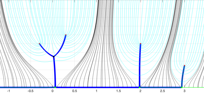
Figure 3: Example of orthogonal flow-lines (level curves of $\mathrm{Re}\,\mathbf{p}(z)$) when $\Omega={\mathrm{Ext}}(\mathfrak{F})$ is simply connected. The Zakharov-Shabat spectrum $\mathfrak{F}=\mathfrak{F}_{{}_{ZS}}\cap{{\mathbb{H}}}$ is shown by blue lines, which are zero level curves of $\mathrm{Im}\,\mathbf{p}(z)$. The red points at the end of blue lines form the set $E$. The level curves of $\mathrm{Re}\,\mathbf{p}(z)$ emanated from $\mathfrak{F}_{{}_{ZS}}$ and from ${\mathbb{R}}$ are shown in light blue and in black respectively. Note the absence of stagnation points in ${{\mathbb{H}}}$, so that the orthogonal flow from ${{\mathbb{H}}}$ to $\mathfrak{F}\cup{\mathbb{R}}$ is everywhere continuous.

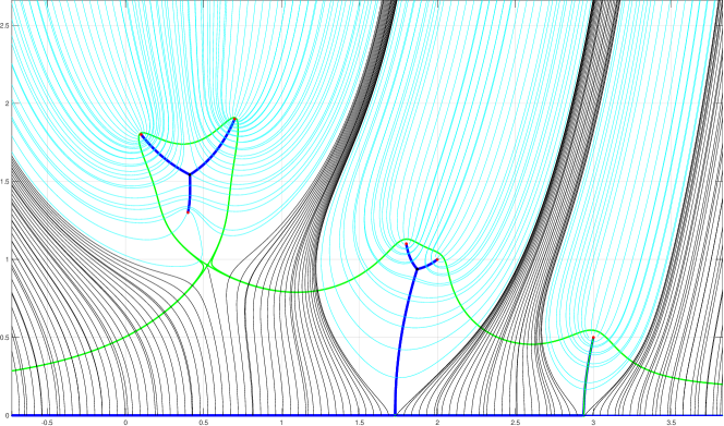
Figure 4: Example of orthogonal flow-lines (level curves of $\mathrm{Re}\,\mathbf{p}(z)$) when $\Omega={\mathrm{Ext}}(\mathfrak{F})$ is not simply connected. The Zakharov-Shabat spectrum $\mathfrak{F}=\mathfrak{F}_{{}_{ZS}}\cap{{\mathbb{H}}}$ is shown by blue lines, which are zero level curves of $\mathrm{Im}\,\mathbf{p}(z)$ . The gradient lines of $\mathrm{Im}\,\mathbf{p}(z)$ emanating from $\mathfrak{F}$ and from ${\mathbb{R}}$ are shown in light blue and in black respectively. Note the stagnation point $z_{0}\in{{\mathbb{H}}}$ (the intersection of green curves) so that the orthogonal flow from ${{\mathbb{H}}}$ to $\mathfrak{F}\cup{\mathbb{R}}$ is discontinuous across the “caustic” (not depicted). The level curve $\mathrm{Im}\,\mathbf{p}(z)=\mathrm{Im}\,\mathbf{p}(z_{0})$ is shown in green.

namely, the zero level set of $V(z)$ in the upper half plane. By the discussion above, also $\mathfrak{F}$ is a forest. See the various (numerically accurate) Figures 2, 3, 4.

Measure and intensity associated with a quasimomentum type quadratic differential.

Let us define $\partial=\frac{1}{2}(\partial_{x}-i\partial_{y})$ (the Wirtinger operator); we then observe that

$${\mathrm{d}}\mathbf{p}=2i\partial V(z){\mathrm{d}}z,\ \ z\in{{\mathbb{H}}}\setminus\mathfrak{F},$$ (2.14)

which extends to a meromorphic differential on $\mathfrak{R}_{L}$ with a pole of order $2$ at $\infty$ on both sheets. According to (2.7),

$${\mathrm{d}}\mathbf{p}(z)=\sqrt{Q(z)}{\mathrm{d}}z=\left(1-\frac{{\mathcal{I}}(\mathfrak{F})}{z^{2}}+\mathcal{O}(z^{-3})\right){\mathrm{d}}z,\ \ z\to\infty,$$ (2.15)

where the constant ${\mathcal{I}}(\mathfrak{F})$ will be called the intensity (average intensity) of the Zakharov–Shabat spectrum $\mathfrak{F}$ and clearly can be obtained by

$${\mathcal{I}}\left(\mathfrak{F}\right):=-\oint_{|z|\gg 1}z\frac{{\mathrm{d}}\mathbf{p}}{2i\pi}=-\mathop{\mathrm{res}}_{z=\infty}\mathbf{p}(z){\mathrm{d}}z,$$ (2.16)

where we integrate in the counterclockwise direction. Here we have extended $\frac{{\mathrm{d}}\mathbf{p}(z)}{{\mathrm{d}}z}$ to the whole plane by Schwartz symmetry in order to define the residue.

On $\mathfrak{F}$ the quadratic differential has the property that $Q{\mathrm{d}}z^{2}>0$ because, as mentioned earlier, the arcs of which $\mathfrak{F}$ is composed are horizontal trajectories. Thus ${\mathrm{d}}\mathbf{p}:=\sqrt{Q}{\mathrm{d}}z$ defines a real differential along $\mathfrak{F}$ and up to a sign, a positive real measure

$${\mathrm{d}}\rho_{{}_{ZS}}(z):=\left|\sqrt{\frac{P_{2N}(z)}{\prod_{j=1}^{N}(z-e_{j})(z-\overline{e_{j}})}}\right|\frac{|{\mathrm{d}}z|}{\pi},$$ (2.17)

with $|{\mathrm{d}}z|$ the standard arc-length parameter. We can express ${\mathrm{d}}\mathbf{p}$ in terms of the measure ${\mathrm{d}}\rho_{{}_{ZS}}$: to this end, we orient $\mathfrak{F}$ and set up a Riemann-Hilbert problem for $\frac{{\mathrm{d}}\mathbf{p}(z)}{{\mathrm{d}}z}=\sqrt{Q}$, which is analytic in ${\mathbb{C}}\setminus(\mathfrak{F}\cup\bar{\mathfrak{F}})$, as follows:

• (jump condition) $\left(\frac{{\mathrm{d}}\mathbf{p}(z)}{{\mathrm{d}}z}\right)_{+}-\left(\frac{{\mathrm{d}}\mathbf{p}(z)}{{\mathrm{d}}z}\right)_{-}=2\pi{\rm e}^{-i\theta(z)}\frac{{\mathrm{d}}\rho_{{}_{ZS}}(z)}{|{\mathrm{d}}z|}$ on $\mathfrak{F}\cup\bar{\mathfrak{F}}$, where $\theta(z)=\arg({\mathrm{d}}z)$ is the angle of the tangent direction to the contour $\mathfrak{F}$ at $z\in\mathfrak{F}$, namely, such that $\sqrt{Q}=|\sqrt{Q}|{\rm e}^{-i\theta(z)}$, and;

• (asymptotics) $\frac{{\mathrm{d}}\mathbf{p}(z)}{{\mathrm{d}}z}=1+O(z^{-2})$ as $z\to\infty$.

By the Sokhotski-Plemelj formula we then have the following representation for $\frac{{\mathrm{d}}\mathbf{p}(z)}{{\mathrm{d}}z}$:

$$\frac{{\mathrm{d}}\mathbf{p}(z)}{{\mathrm{d}}z}=1+i\int_{\mathfrak{F}}\left(\frac{1}{\overline{w}-z}-\frac{1}{w-z}\right){\mathrm{d}}\rho_{{}_{ZS}}(w),$$ (2.18)

from which it follows that

$${\mathcal{I}}(\mathfrak{F})=2\int_{\mathfrak{F}}\mathrm{Im}\,(w){\mathrm{d}}\rho_{{}_{ZS}}(w).$$ (2.19)

Here we note that, according to results of [32], Section 3.5, $\frac{{\mathrm{d}}\rho_{{}_{ZS}}(z)}{|{\mathrm{d}}z|}$ coincides with the density of states (DOS) $u(z)$, i.e., with the solution of the (1.9) for the fNLS soliton condensate with $\Gamma^{+}=\mathfrak{F}$. Moreover, the expression (2.19) for the average intensity ${\mathcal{I}}(\mathfrak{F})$ coincides with the average conserved density $I_{1}$ from Corollary 1.2, [32] for this condensate. It also coincides with the average intensity of finite gaps solutions of the fNLS on $\mathfrak{R}_{L}$ ([7]).

The $S$–property of the contours.

The arcs of $\mathfrak{F}$ have the so–called $S$–property, introduced by H. Stahl in [30]. At each point $z$ in the (relative) interior of a smooth arc of $\mathfrak{F}$ we have two opposite normal directions which we denote by ${\bf n}_{\pm}(z)$. Then the $S$–property is the statement that the two normal derivatives of $V=\mathrm{Im}\,\mathbf{p}(z)$ coincide:

$$\frac{\partial}{\partial{\bf n}_{+}}V-\frac{\partial}{\partial{\bf n}_{-}}V=0.$$ (2.20)

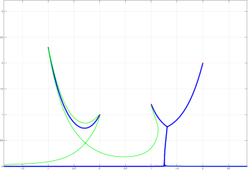
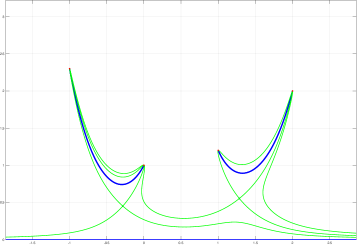
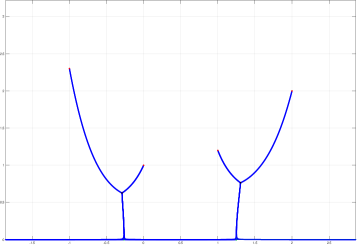
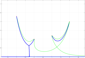
Figure 2: Examples of four Zakharov–Shabat spectra for the same configuration of anchor set $E$. Indicated also the stagnation points and the trajectories through them.

3 Generalized quasimomenta associated to compact sets

Let $\mathcal{K}\subset\overline{{{\mathbb{H}}}}$ be a poly-continuum. We recall that the “exterior” of $\mathcal{K}$, denoted ${\mathrm{Ext}}(\mathcal{K}){:=\Omega}$, is the (unique) unbounded connected component of the complement of $\mathcal{K}$ in ${{\mathbb{H}}}$ and the “interior” of $\mathcal{K}$, denoted ${\mathrm{Int}}(\mathcal{K})$ is the (necessarily compact) complement of ${\mathrm{Ext}}(\mathcal{K})$. The “exterior boundary” of $\mathcal{K}$ is then the boundary of ${\mathrm{Ext}}(\mathcal{K})$, which is a subset, in general, of the boundary of $\mathcal{K}$. Consider the Dirichlet problem

Problem 3.1

Let $G(z)=G(z;\mathcal{K}):{{\mathbb{H}}}\to{\mathbb{R}}_{+}$ be the unique function satisfying the conditions

1. $G(z)$ is continuous in ${{\mathbb{H}}}\cup{\mathbb{R}}$;

2. $G(z)$ is harmonic and bounded in ${{\mathbb{H}}}\setminus\mathcal{K}$ ;

3. $G\big{|}_{\mathcal{K}\cup{\mathbb{R}}}\equiv\mathrm{Im}\,z$.

We observe that any continuum (and so poly-continuum) is regular for the Dirichlet problem, meaning that the Green function of the complement is continuous up to the boundary and is zero therein. This follows from the characterization in [28], App A.2, Theorem 2.1, of regular points in terms of the Wiener condition, which is easily shown to hold at all points of the continuum.

Since $\mathrm{Im}\,(z)$ is harmonic in ${{\mathbb{H}}}$ we have $G\equiv\mathrm{Im}\,(z)$ on ${\mathrm{Int}}(\mathcal{K})$ (which is larger than $\mathcal{K}$ in general), so that the only important information is contained in the shape of ${\mathrm{Int}}(\mathcal{K})$. Therefore, without loss of generality, we assume henceforth that $\mathcal{K}={\mathrm{Int}}(\mathcal{K})$. Let $H$ be a (multi-valued) harmonic conjugate function to $G$ in ${\mathrm{Ext}}(\mathcal{K})$. The function $H$ has additive multi-valuedness under the harmonic continuation in ${\mathrm{Ext}}(\mathcal{K})$. By performing some additional branchcuts, $H$ becomes single valued in the complement, see Section 3.1.1. The following properties hold:

1. There is a positive measure ${\mathrm{d}}\rho_{\mathcal{K}}(z)=u(z)|{\mathrm{d}}z|$ supported on $\partial\mathcal{K}$ such that

   $$G(z;\mathcal{K})=\int_{\partial\mathcal{K}}\ln\left|\frac{z-\overline{w}}{z-w}\right|{\mathrm{d}}\rho_{\mathcal{K}}(w).$$ (3.1)

   Consequently, up to appropriate choices of the branches of the logarithm

   $$g(z;\mathcal{K})=iG(z;\mathcal{K})-H(z;\mathcal{K})=i\int_{\partial\mathcal{K}}\ln\left(\frac{z-\overline{w}}{z-w}\right){\mathrm{d}}\rho_{\mathcal{K}}(w),$$ (3.2)

   where the logarithm can be defined unambiguously, see Section 3.1.1.

2. if we define the generalized quasimomentum by

   $$\mathcal{P}(z;\mathcal{K}):=z-g(z)=z-iG(z;\mathcal{K})+H(z;\mathcal{K})=U(z)+iV(z),$$ (3.3)

   then it has the property that:

   1. $\mathcal{P}$ is analytic (multi-valued) in ${\mathrm{Ext}}(\mathcal{K})$;

   2. $V=\mathrm{Im}\,(\mathcal{P})\equiv 0$ on $\mathcal{K}\cup{\mathbb{R}}$

   3. as $|z|\to\infty$ we have (as a convergent series)

      $$\mathcal{P}(z;\mathcal{K})=z+\frac{2\int_{\partial\mathcal{K}}\mathrm{Im}\,(w){\mathrm{d}}\rho_{\mathcal{K}}(w)}{z}+\sum_{j=2}^{\infty}\frac{2}{z^{j}}\int_{\partial\mathcal{K}}\mathrm{Im}\,(w^{j}){\mathrm{d}}\rho_{\mathcal{K}}(w).$$ (3.4)

The fact that the density $u(z)$ of the measure ${\mathrm{d}}\rho_{\mathcal{K}}$ is positive at any $z$ on the (smooth) exterior boundary $\partial\mathcal{K}$ is a consequence of the minimum principle for $\mathrm{Im}\,\mathcal{P}$ and the fact that $\mathrm{Im}\,\mathcal{P}\equiv 0$ only on ${\mathrm{Int}}(\mathcal{K})$.

Definition 3.2

The (generalized) intensity of $\mathcal{K}$ is the quantity

$${\mathcal{I}}(\mathcal{K}):=2\int_{\partial\mathcal{K}}\mathrm{Im}\,(w){\mathrm{d}}\rho_{\mathcal{K}}(w).$$ (3.5)

Notice that (3.5) coincides with the formula (2.19) when $\mathcal{K}=\mathfrak{F}$ and also coincides with the average intensity (1.11) of the fNLS soliton condensate defined by $\Gamma^{+}=\mathfrak{F}$. Moreover, according to [32], the averaged conserved densities of the fNLS soliton condensate, defined by $\mathcal{K}$, coincide with the coefficients of the $\mathcal{P}(z;\mathcal{K})$ Laurent expansion at $z=\infty$ given by (3.4).

There are several equivalent representation of ${\mathcal{I}}(\mathcal{K})$. The first is obtained using the defining property of $G(z;\mathcal{K})\equiv\mathrm{Im}\,z$ on $\mathcal{K}$. Integrating over $\partial\mathcal{K}$ this identity against ${\mathrm{d}}\rho_{\mathcal{K}}$ we obtain

$${\mathcal{I}}(\mathcal{K})=2\int_{\partial\mathcal{K}}G(z;\mathcal{K}){\mathrm{d}}\rho_{\mathcal{K}}(z)=2\iint_{\partial\mathcal{K}\times\partial\mathcal{K}}\ln\left|\frac{z-\overline{w}}{z-w}\right|{\mathrm{d}}\rho_{\mathcal{K}}(z){\mathrm{d}}\rho_{\mathcal{K}}(w)=$$ (3.6)

$$4\int_{\partial\mathcal{K}}\mathrm{Im}\,(w){\mathrm{d}}\rho_{\mathcal{K}}(w)-2\iint_{\partial\mathcal{K}\times\partial\mathcal{K}}\ln\left|\frac{z-\overline{w}}{z-w}\right|{\mathrm{d}}\rho_{\mathcal{K}}(z){\mathrm{d}}\rho_{\mathcal{K}}(w)=-2J_{0}(\rho_{\mathcal{K}}).$$ (3.7)

Here the last expression in the first line represents the free Green energy of $\rho_{\mathcal{K}}$ ([28]), whereas the expression in the second line represent the weighted Greens’ energy $J_{0}$, see Section 1.3, multiplied by $-2$. On the other hand the measure ${\mathrm{d}}\rho_{\mathcal{K}}$ is the distributional Laplacian

$$\triangle G(z;\mathcal{K})=-2\pi{\mathrm{d}}\rho_{\mathcal{K}}$$ (3.8)

of $G(z;\mathcal{K})$ and then using the Green formula we also have

$${\mathcal{I}}(\mathcal{K})=\frac{2\pi}{i}\int_{{\mathrm{Ext}}(\mathcal{K})}\overline{\partial}G(z;\mathcal{K}){\mathrm{d}}\overline{z}\wedge\partial G(z;\mathcal{K}){\mathrm{d}}z=\pi\int_{{\mathrm{Ext}}(\mathcal{K})}|g^{\prime}(z)|^{2}{\mathrm{d}}x{\mathrm{d}}y=\pi D_{\mathcal{K}},$$ (3.9)

where $D_{\mathcal{K}}$ denotes the the Dirichlet energy of the solution $G(z;\mathcal{K})$ of the Dirichlet Problem 3.1. Thus, equation (3.9) shows that the intensity $\mathcal{I}(\mathcal{K})$ coincides with the Dirichlet $D_{\mathcal{K}}$ up to a factor $\pi$. That is why sometimes we also refer to ${\mathcal{I}}(\mathcal{K})$ as to Dirichlet energy of $\mathcal{K}$.

3.1 The generalized quasimomentum and the uniformization theorem

The relationship between the generalized quasimomentum $\mathcal{P}$ and the uniformizing map is elucidated by the following proposition.

Proposition 3.3

Suppose that $\Omega={\mathrm{Ext}}(\mathcal{K})$ is simply connected in ${{\mathbb{H}}}$; then $\mathcal{P}(z;\mathcal{K})$ is the uniformizing map of $\Omega$ to ${{\mathbb{H}}}$ with the normalization condition that $\mathcal{P}(z;\mathcal{K})=z+\mathcal{O}(z^{-1})$ as $z\to\infty$. In particular, there are no points $z\in\Omega$ with $\mathcal{P}^{\prime}(z;\mathcal{K})=0$, i.e., the points with $\nabla G(z;\mathcal{K})=0$.

Proof. Let us temporarily denote by $\varphi(z)$ an uniformizing map of the assumed simply-connected domain ${\mathrm{Ext}}(\mathcal{K})$ to the upper half-plane (the existence of which is guaranteed by the Riemann uniformization theorem). We can fix it uniquely if we impose $\varphi(\infty)=\infty$ and then normalize (by real–multiplication and addition of a constant) so that $\varphi(z)=z+\mathcal{O}(z^{-1})$. Since $\varphi$ is a uniformizing map, we have $\mathrm{Im}\,(\varphi)\bigg{|}_{{\mathbb{R}}\cup\partial{\mathrm{Ext}}(\mathcal{K})}\equiv 0$. Thus the function $G(z):=\mathrm{Im}\,(z-\varphi(z))$ solves Problem 3.1 in ${\mathrm{Ext}}(\mathcal{K})$. We can extend it to be identically equal to $G\equiv\mathrm{Im}\,(z)$ in the ${\mathrm{Int}}(K)$ and then it must coincide with the solution of the same Problem 3.1. Thus $\mathrm{Im}\,\varphi(z)=\mathrm{Im}\,(z)-G$. The harmonic conjugate function of $G$, denoted by $H$, is uniquely defined (up to additive constant) in ${\mathrm{Ext}}(\mathcal{K})$ because of the assumption that ${\mathrm{Ext}}(\mathcal{K})$ is simply connected and hence $\varphi(z)=z-iG+H$. Since $G$ is precisely the solution of Problem 3.1, then the equality $\varphi=\mathcal{P}$ follows from (3.3). $\blacksquare$

3.1.1 The non simply connected case

Even if ${{\mathbb{H}}}\setminus\mathcal{K}$ is not simply connected, the map $\xi=\mathcal{P}(z;\mathcal{K})$ can be used to describe a useful univalent function, provided we perform some additional slits.

Proposition 3.4

Let us denote by $\mathcal{K}_{\ell}$, $\ell=1,\dots,k,$ the connected components of $\mathcal{K}$ not meeting ${\mathbb{R}}$ and by $\mathcal{K}_{0}$ the remaining connected component of $\mathcal{K}\cup{\mathbb{R}}$. Then $\mathcal{P}^{\prime}(z;\mathcal{K})=\frac{{\mathrm{d}}\mathcal{P}(z;\mathcal{K})}{{\mathrm{d}}z}$ has $k$ zeros (“stagnation points”), counted with multiplicity, in ${{\mathbb{H}}}\setminus\mathcal{K}$.

We are only sketching the elementary proof. It can be established using the Argument Principle, i.e., calculating the increment of $\arg\mathcal{P}^{\prime}(z)$ along a contour $\gamma$ that closely follows the boundary of $\Omega={\mathrm{Ext}}(\mathcal{K})$ (but also using elementary Morse theory applied to $\mathrm{Im}\,\mathcal{P}$). For example, let $\gamma$ consist of the union of level curves $\mathrm{Im}\,\mathcal{P}(z)=M$ and $\mathrm{Im}\,\mathcal{P}(z)=m$, where $M>0$ is sufficiently large and $m>0$ is sufficiently small. Due to (3.4), the increment of $\arg\mathcal{P}^{\prime}(z)$ along the “semicircle” $\mathrm{Im}\,\mathcal{P}(z)=M$ is very small. Along the level curves of $\mathrm{Im}\,\mathcal{P}(z)$, we have $\arg\mathcal{P}^{\prime}(z)=-\arg{\mathrm{d}}z$. Thus, we have a small increment of $\arg\mathcal{P}^{\prime}(z)$ along the level curve $\mathrm{Im}\,\mathcal{P}(z)=m$ near the remaining part of the outer boundary of $\Omega$. However, the increment of $\arg\mathcal{P}^{\prime}(z)$ along $\mathrm{Im}\,\mathcal{P}(z)=m$ around each of the remaining components of $\mathcal{K}$ is $2\pi$, which yields the desired statement. Similar result was proven in [25], Section 26, for critical points of a Green function of a multiply connected region.

Remark 3.5

The terminology of ”stagnation points” comes from the interpretation of the integral lines of the gradient of $G(z;\mathcal{K})$ as flow-lines of a two–dimensional fluid and the fact that they are points where the gradient flow has a fixed point.

Denote the stagnation points of Proposition 3.4 by $z_{1},\dots,z_{s}$ with multiplicies $m_{1},\dots,m_{s}$, $\sum_{j=1}^{s}m_{j}=k$.

From each $z_{j}$ we take all the arcs of steepest descent trajectories of $\Phi=\mathrm{Im}\,\mathcal{P}$ up to either another stagnation point or $\mathcal{K}\cup{\mathbb{R}}$. Denote by $\Sigma:=\bigcup_{d}\sigma_{d}$ the union of these arcs.

We claim that there are $e:=\sum_{j=1}^{s}(m_{j}+1)$ such arcs in $\Sigma$. Indeed we have taken all the steepest descent trajectories from the points $z_{j}$ (of which there are $(m_{j}+1)$). In the generic (Morse) case there are precisely $2k$ arcs and all $m_{j}=1$. We want to show

Proposition 3.6

The domain $\mathcal{D}:={{\mathbb{H}}}\setminus(\mathcal{K}\cup\Sigma)$ is connected and simply connected and the map $\xi=\mathcal{P}(z;\mathcal{K})$ is univalent on $\mathcal{D}$ and maps it to the upper half $\xi$–plane minus finitely many vertical segments with one endpoint on the real axis.

For example, if all stagnation points are simple, then the system of cuts $\Sigma$ consists of the union of the two arcs of steepest descent from each such point. Then, each such pair of arcs is represented in the $\xi$–plane by a pair of vertical segments of the same length. We first prove the claims of connectedness.

Lemma 3.7

The set ${{\mathbb{H}}}\setminus(\mathcal{K}\cup\Sigma)$ is connected and simply connected.

Proof. This is the same as showing that $\mathcal{K}\cup\Sigma$ is a tree (in the sense of graph theory), with set $\mathcal{V}$ of $k+s+1$ vertices consisting of one node associated to each of the connected components $\mathcal{K}_{0},\dots\mathcal{K}_{k}$, and one for each stagnation point $z_{1},\dots,z_{s}$. The set of edges $\mathcal{E}$ consists of the $\sum_{j=1}^{s}(m_{j}+1)=s+k$ arcs in $\Sigma$.

First we show that ${{\mathbb{H}}}\setminus(\mathcal{K}\cup\Sigma)$ is connected, i.e., it has only one connected component; if not, then at least one component, say $\mathscr{D}$, is bounded (since $\Sigma$ is compact and the only non-compact component is $\mathcal{K}_{0}\supset{\mathbb{R}}$). The boundary of such $\mathscr{D}$ consists of pieces of boundaries of various $\mathcal{K}_{\ell}$’s, and edges of $\Sigma$ (and corresponds to a loop in the graph).

The function $\Phi=\mathrm{Im}\,\mathcal{P}$ is harmonic in $\mathscr{D}$ and thus should take its maximum on the boundary of $\mathscr{D}$; this maximum must precisely occur at one of the stagnation points on $\partial\mathscr{D}$ (because $\Phi=0$ on $\mathcal{K}$). Suppose $z_{0}$ is the maximum on the boundary. However $z_{0}$ is a saddle point and the boundary of $\mathscr{D}$ near $z_{0}$ must consist of two branches of steepest descent trajectories, which leaves at least one steepest ascent trajectory from $z_{0}$ going into $\mathscr{D}$. So $z_{0}$ could not be a maximum and we have reached the desired contradiction.

Note that since the boundary of $\mathscr{D}$ would constitute a loop in the graph $\mathcal{K}\cup\Sigma$, the above argument shows that $\mathcal{K}\cup\Sigma$ has no loops and hence it is either a tree or a forest (union of disjoint trees). We want to exclude the latter case. This is a simple counting argument with the Euler characteristic: for each tree we must have one less edge than vertices. Since we have a total of $k+s+1$ vertices already and $k+s$ edges, the graph $\mathcal{K}\cup\Sigma$ must be connected. Thus, ${{\mathbb{H}}}\setminus(\mathcal{K}\cup\Sigma)$ must be simply connected. $\blacksquare$

Proof of Proposition 3.6.

The domain $\mathcal{D}:={{\mathbb{H}}}\setminus(\mathcal{K}\cup\Sigma)$ is connected and simply connected and also, by Proposition 3.3, does not contain any zero of $\mathcal{P}^{\prime}$; thus $\mathcal{P}$ can be defined as a univalent and single–valued analytic function. All boundaries of $\mathcal{K}_{0}\supset{\mathbb{R}},\mathcal{K}_{1},\dots,\mathcal{K}_{k}$ are mapped to segments of the real $\xi$–axis, while all the edges of $\Sigma$, by construction being unions of gradient lines of $\mathrm{Im}\,\xi=\mathrm{Im}\,\mathcal{P}$ must have constant $\mathrm{Re}\,\xi=\mathrm{Re}\,\mathcal{P}$ and hence are mapped to vertical slits. Along these slits are the images of stagnation points. In particular, the tip of each slit correspond to a stagnation point. Each arc $\sigma_{h}$ of $\Sigma$ is mapped to a sub-segment of one of the sides of a slit. $\blacksquare$

In the generic case where $\Phi$ is a (nondegenerate) Morse function [24], all the stagnation points are simple, and each of the $2k$ arcs $\sigma_{j}$ connects a stagnation point to one of the components of $\mathcal{K}\cup{\mathbb{R}}$, the image $\mathcal{P}(\mathcal{D})$ is simplest. It consists of ${{\mathbb{H}}}$ with $2k$ pairs of vertical slits with the sides of the slits identified in pairs, and the apex of each pair representing the same stagnation point.

Of course the statements of this section apply equally well to the Zakharov–Shabat spectra; we will however keep the notation $\zeta=\mathbf{p}(z)$ for the uniformizing map in that case. The Zakharov–Shabat case has the additional property of the existence of a measure preserving involution, which is a property ultimately equivalent to Stahl $S$–property.

4 Jenkins’ interception property and the Dirichlet energy

In this section we prove a comparison theorem between the Dirichlet energies of two sets. We will use as reference a set $\mathfrak{F}$ such that ${{\mathbb{H}}}\setminus\mathfrak{F}$ is connected and $\mathfrak{F}$ consists of a finite union of smooth arcs, so that at each relative interior point of each arc we can define the tangent and the two normal directions. With a slight abuse of notation, we will denote by $\mathbf{p}$ the generalized quasimomentum of $\mathfrak{F}$. In general this set $\mathfrak{F}$ does not have the S-property (2.20), that is, the two normal derivatives of $v=\mathrm{Im}\,\mathbf{p}$ from the opposite sides are not necessarily equal to each other. For each point $z$ in the relative interior of one of the arcs there are exactly two orthogonal flow-lines of the gradient of $v$, and the one in the direction of the larger $\frac{\partial\mathrm{Im}\,\mathbf{p}(z)}{\partial{\bf n}_{\pm}}$, will be called dominant orthogonal trajectory and denoted $\mathcal{L}^{\perp}_{d}(z)$. The remaining orthogonal trajectory will be called recessive and denoted $\mathcal{L}^{\perp}_{r}(z)$. In the case where the normal derivatives are equal, any of the two orthogonal trajectories can be considered as dominant.

Definition 4.1

We say that a poly-continuum $\mathcal{K}$ has Jenkins’ interception property with respect to $\mathfrak{F}$ if $\mathcal{L}^{\perp}_{d}(z)\cap\mathcal{K}\neq\emptyset$ for all $z$ in the relative interior of every arc of $\mathfrak{F}$.

In the case when $\mathfrak{F}$ represents a Zakharov–Shabat spectrum (i.e. it has the $S$-property), the Jenkins’ interception property means that for every $z$ in the interior of $\mathfrak{F}$ at least one orthogonal trajectory $\mathscr{L}^{\perp}(z)$ intersects $\mathcal{K}$. The main results of this paper are based on the following theorem.

Theorem 4.2

If a poly-continuum $\mathcal{K}$ has Jenkins’ interception property with respect to $\mathfrak{F}$ (Def. 4.1) then

$${\mathcal{I}}(\mathfrak{F})\leq{\mathcal{I}}(\mathcal{K}).$$ (4.1)

Moreover, the equality in (4.1) implies $\mathcal{K}=\mathfrak{F}$.

Theorem 4.2 implies that a small deformation of $\mathfrak{F}$ in the dominant direction increases ${\mathcal{I}}(\mathfrak{F})$. Here “small” means a small and smooth displacement of a point $z$ in the interior of $\mathfrak{F}$ as well as a small variation in the normal direction ${\bf n}(z)$ to $\mathfrak{F}$. In fact, these deformations do not have to be small as long as the connectivity (the topology) of $\mathfrak{F}$ is preserved. The above arguments show that any $\mathfrak{F}$ with S-property is a local minimum of the Dirichlet energy functional ${\mathcal{I}}(\mathfrak{F})$. Moreover, it must be the global minimum of ${\mathcal{I}}(\mathfrak{F})$ in the subclass of compacts in ${\mathbb{K}}_{E}$ with the same connectivity as $\mathfrak{F}$, i.e., in the class of connectivity perserving deformations.

The proof of Theorem 4.2 is based on the “length–area method”, and generalizes the result of [14]. For a given $\mathcal{K}$ we have the function $\mathcal{P}(z)=\mathcal{P}(z;\mathcal{K})$ defined as a multi-valued analytic function on ${{\mathbb{H}}}\setminus\mathcal{K}$ with purely real additive multivaluedness, i.e. the analytic continuation along any closed loop in ${{\mathbb{H}}}\setminus\mathcal{K}$ yields the same germ of analytic function plus a real constant (recall our running assumption that $\mathcal{K}={\mathrm{Int}}(\mathcal{K})$).

From the asymptotics of the quasimomenta (3.4) it follows that both $\mathbf{p}(z),\mathcal{P}(z)$ are invertible for sufficiently large $|z|$.

The proof of Theorem 4.2 is preceeded by several lemmas. We start by denoting by $R_{L}$ the rectangle in the $\zeta=u+iv$–plane of area $2L^{2}$:

$$R_{L}:=\Big{\{}u\in[-L,L],\ v\in[0,L]\Big{\}}.$$ (4.2)

Let us define a deformed rectangle ${\mathcal{R}}_{L}$ in the $z$-plane as the region bounded by the pre-images of the left/right/top sides of $R_{L}$ and the real axis of $\zeta=\mathbf{p}(z)$. Similarly we define the deformed rectangle $\mathscr{R}_{L}$ in the $\xi$–plane, where $\xi=\mathcal{P}(z;\mathcal{K})$. Note that ${\mathcal{R}}_{L}$ in the $z$–plane contains all of $\mathfrak{F}$ for $L$ sufficiently large, see Fig. 5.

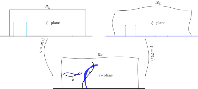
Figure 5: The three rectangles.

The vertical lines in the $\zeta$–plane correspond to the foliation by the orthogonal flow of $v=\mathrm{Im}\,\mathbf{p}$ in the $z$–plane.

We are interested in the single–valued analytic differential $\frac{{\mathrm{d}}\mathcal{P}}{{\mathrm{d}}z}$ on ${{\mathbb{H}}}\setminus\mathcal{K}$. Note that if $z$ is any interior point to $\mathcal{K}$ (in the topological sense), then ${\mathrm{d}}\mathcal{P}/{\mathrm{d}}z=0$ in any small disk centered at $z$ and contained in $\mathcal{K}$.

The conformal area form and metric induced by $\mathcal{P}$ are given by

$${\mathrm{d}}A:=\hat{\rho}^{2}{\mathrm{d}}^{2}z,\ \ \ \ \hat{\rho}:=\left|\frac{{\mathrm{d}}\mathcal{P}}{{\mathrm{d}}z}\right|,\ \ \ {\mathrm{d}}^{2}z:={\mathrm{d}}x{\mathrm{d}}y,\ \ {\mathrm{d}}s=\hat{\rho}|{\mathrm{d}}z|.$$ (4.3)

Note that in this metric any point in the interior of the same connected component of $\mathcal{K}$ is at zero distance from any other point in the same class.

By the change of variable formula the area form ${\mathrm{d}}A$ in the $z$-plane is transformed to the $\zeta$-plane as follows:

$$\mathbf{p}^{\star}({\mathrm{d}}A)=\rho^{2}(u,v){\mathrm{d}}^{2}\zeta,\ \ \ \rho(u,v):=\hat{\rho}\left|\frac{{\mathrm{d}}z}{{\mathrm{d}}\mathbf{p}}\right|=\left|\frac{{\mathrm{d}}\mathcal{P}}{{\mathrm{d}}\mathbf{p}}\right|,\quad\zeta=u+iv,\ \ {\mathrm{d}}^{2}\zeta:={\mathrm{d}}u{\mathrm{d}}v.$$ (4.4)

The main strategy is to compute an upper and lower bound for the integral

$$\mathscr{A}_{L}:=\iint_{R_{L}}{\rho^{2}(u,v)}{\mathrm{d}}^{2}\zeta,$$ (4.5)

which represents area of the image $\mathscr{R}_{L}$ of $R_{L}$ under the map $\mathcal{P}\circ\mathbf{p}^{-1}(R_{L})$.

Lower bound for (4.5).

Let us partition $[-L,L]=U^{+}\sqcup U^{-}\sqcup U^{0}$ into disjoint sets. To describe them let $\mathfrak{F}^{\circ}$ denote the union of the relative interiors of all arcs of $\mathfrak{F}$ (i.e. all except the meeting points of two or more smooth arcs) and observe that the image $\zeta=\mathbf{p}(z)$ of every point $z\in\mathfrak{F}^{\circ}$ appears exactly twice on $[-L,L]$, say at $u$ and $u^{\star}$. Our convention is such that $u$ corresponds to the side of the dominant trajectory $\mathcal{L}^{\perp}_{d}(z)$ and we call such $u$’s “dominant”. Viceversa, points in the relative interior of ${\mathbb{R}}\setminus\mathfrak{F}$ appear only once in $[-L,L]$. Then we define the dominant subset by

$$U^{+}=\left\{u\in[-L,L]:\exists w\in\mathfrak{F}^{\circ}:\ \ \mathbf{p}(w)=u,\text{ $u$ dominant}\right\}.$$ (4.6)

The recessive subset is similarly defined

$$U^{-}=\left\{u\in[-L,L]:\exists w\in\mathfrak{F}^{\circ}:\ \ \mathbf{p}(w)=u^{\star},\text{ $u$ dominant (i.e. $u^{\star}$ recessive) }\right\}.$$ (4.7)

Finally we denote $U^{0}=[-L,L]\setminus\overline{U^{+}\cup U^{-}}$; this includes the points on ${\mathbb{R}}$.

Lemma 4.3

Let $L$ be sufficiently large. For any $u\in U^{+}\cup U^{-}$ we denote by $w\in\mathfrak{F}^{\circ}$ the corresponding point in the $z$–plane. For almost every $u\in[-L,L]$ we have

$$\int_{0}^{L}\rho(u,v){\mathrm{d}}v\geq\mathrm{Im}\,\left(\mathcal{P}(\mathbf{p}^{-1}(u+iL))\right)~~\text{when }~~u\in U^{0}$$ (4.8)

$$\int_{0}^{L}\rho(u,v){\mathrm{d}}v\geq\mathrm{Im}\,\left(\mathcal{P}(\mathbf{p}^{-1}(u+iL))+\mathcal{P}(w)\right)~~\text{when }~~u\in U^{+},$$ (4.9)

$$\int_{0}^{L}\rho(u,v){\mathrm{d}}v\geq\mathrm{Im}\,\left(\mathcal{P}(\mathbf{p}^{-1}(u+iL))-\mathcal{P}(w)\right)~~\text{when }~~u\in U^{-}.$$ (4.10)

Proof. Consider first the case where $U^{0}\ni u=\mathbf{p}(w)$, where $w\in{\mathbb{R}}$. The integral then computes the total variation of $\mathcal{P}$ along the orthogonal trajectory $\gamma_{w}^{w_{1}}:=\mathbf{p}^{-1}(u+i[0,L])$, which starts from the point $w=\mathbf{p}^{-1}(u)\in{\mathbb{R}}$ and ends at $w_{1}=\mathbf{p}^{-1}(u+iL)$:

$$\int_{0}^{L}\rho(u,v){\mathrm{d}}v=\int_{0}^{L}\left|\frac{{\mathrm{d}}\mathcal{P}}{{\mathrm{d}}z}\right|\left|\frac{{\mathrm{d}}z}{{\mathrm{d}}\mathbf{p}}\right||{\mathrm{d}}\zeta|=\int_{\gamma_{w}^{w_{1}}}\left|\frac{{\mathrm{d}}\mathcal{P}}{{\mathrm{d}}z}\right||{\mathrm{d}}z|.$$ (4.11)

Since $w\in{\mathbb{R}}$, we have in particular $\mathrm{Im}\,\mathcal{P}(w)=0$ , and we conclude that the total variation is certainly at least equal to $\mathrm{Im}\,\mathcal{P}(w_{1})=\mathrm{Im}\,\mathcal{P}(\mathbf{p}^{-1}(u+iL))$. This establishes the inequality (4.8) in this case.

Let us now assume that $u\in U^{+}$ so that $\mathcal{L}_{d}^{\perp}(w)\cup\mathcal{K}\neq\emptyset$. Let $x_{0}$ be the first intersection point (with $\mathcal{K}$) along $\mathcal{L}_{d}^{\perp}(w)$ as it leaves $w\in\mathfrak{F}$ and $x_{1}$ be the last such point (it may happen that $x_{0}=x_{1}$). Then the total variation of $\mathcal{P}$ can be bounded below by the sum of $\mathrm{Im}\,\mathcal{P}(\mathbf{p}^{-1}(u+iL))$ on $[x_{1},\mathbf{p}^{-1}(u+iL)]$ and $\mathrm{Im}\,\mathcal{P}(w)$ on $[w,x_{0}]$, which proves the second inequality (4.8) (note $\mathrm{Im}\,\mathcal{P}=0$ on $\mathcal{K}$).

Now consider a point $u\in U^{-}$. Assume the corresponding recessive orthogonal trajectory $\mathcal{L}^{\perp}(w)$ does not intersects $\mathcal{K}$. Then the total variation of $\mathcal{P}$ can be bounded below by the sum of $\mathrm{Im}\,\mathcal{P}(\mathbf{p}^{-1}(u+iL))-\mathrm{Im}\,\mathcal{P}(w)$ on $[w,\mathbf{p}^{-1}(u+iL)]$. If the recessive trajectory $\mathcal{L}^{\perp}(w)$ does intersect $\mathcal{K}$, then we recover the second inequality in (4.8), which implies the third inequality since $\mathrm{Im}\,\mathcal{P}\geq 0$ in ${{\mathbb{H}}}$. $\blacksquare$

Lemma 4.4

Let $L$ be sufficiently large. Then for almost every $u\in[-L,L]$:

$$\mathrm{Im}\,\mathcal{P}(\mathbf{p}^{-1}(u+iL))=L+\frac{({\mathcal{I}}(\mathfrak{F})-{\mathcal{I}}(\mathcal{K}))L}{(L^{2}+u^{2})}+\mathcal{O}(L^{-2}).$$ (4.12)

Proof. Since

$$\mathbf{p}(z)=z+\frac{{\mathcal{I}}(\mathfrak{F})}{z}+\mathcal{O}(z^{-2}),~\mathcal{P}(z)=z+\frac{{\mathcal{I}}(\mathcal{K})}{z}+\mathcal{O}(z^{-2}),$$ (4.13)

we have

$$\mathcal{P}(\mathbf{p}^{-1}(\zeta))=\zeta-\frac{{\mathcal{I}}(\mathfrak{F})-{\mathcal{I}}(\mathcal{K})}{\zeta}+\mathcal{O}(\zeta^{-2}).$$ (4.14)

The statement is a consequence of (4.14). $\blacksquare$

Lemma 4.5

In the large $L$ limit the area $\mathscr{A}_{L}$ of $\mathscr{R}_{L}$ satisfies

$$\mathscr{A}_{L}=\iint_{R_{L}}{\rho(u,v)}^{2}{\mathrm{d}}^{2}\zeta\geq 2L^{2}+\pi({\mathcal{I}}(\mathfrak{F})-{\mathcal{I}}(\mathcal{K}))+\mathcal{O}(L^{-1}).$$ (4.15)

Proof. By the definition of $U^{\pm}$, there is a bijection $U^{+}\mapsto U^{-}$ given by $u\mapsto u^{\star}$. The pull back of $du$ from $U^{-}$ to $U^{+}$ yields

$$\phi(u)du=\dfrac{\frac{\partial\mathrm{Im}\,\mathbf{p}}{\partial n_{-}}}{\frac{\partial\mathrm{Im}\,\mathbf{p}}{\partial n_{+}}}du\leq du,$$ (4.16)

where $n_{+}$ is the normal vector to $\mathfrak{F}^{\circ}$ in the dominant direction. Now, according to Lemmas 4.3,4.4, we have

$$\int_{-L}^{L}\int_{0}^{L}\rho(u,v){\mathrm{d}}v{\mathrm{d}}u\geq\int_{U^{+}}\mathrm{Im}\,\left(\mathcal{P}(\mathbf{p}^{-1}(u+iL))+\mathcal{P}(w)\right)du+\int_{U^{-}}\mathrm{Im}\,\left(\mathcal{P}(\mathbf{p}^{-1}(u+iL))-\mathcal{P}(w)\right)du$$ (4.17)

$$+\int_{U^{0}}\mathrm{Im}\,\mathcal{P}(\mathbf{p}^{-1}(u+iL)du=\int_{-L}^{L}\left(L+\frac{[{\mathcal{I}}(\mathfrak{F})-{\mathcal{I}}(\mathcal{K})]L}{(L^{2}+u^{2})}+\mathcal{O}(L^{-2})\right){\mathrm{d}}u+\int_{U^{+}}\mathrm{Im}\,\mathcal{P}(\mathbf{p}^{-1}(u)))\left(1-\phi(u)\right)du\geq$$ (4.18)

$$2L^{2}+\frac{\pi}{2}[{\mathcal{I}}(\mathfrak{F})-{\mathcal{I}}(\mathcal{K})]+\mathcal{O}(L^{-1}),$$ (4.19)

where we used (4.16) and the fact that $U^{+}\cup U^{-}\cup U^{0}=[-L,L]$ up to a measure zero set.

We rewrite the latter inequality as follows

$$\iint_{R_{L}}\Big{(}\rho(u,v)-1\Big{)}{\mathrm{d}}^{2}\zeta\geq\frac{\pi}{2}[{\mathcal{I}}(\mathfrak{F})-{\mathcal{I}}(\mathcal{K})]+\mathcal{O}(L^{-1}).$$ (4.20)

To finally estimate the area (which is the integral of the square of $\rho$) we proceed as follows:

$$\mathscr{A}_{L}-2L^{2}=\iint_{R_{L}}\Big{(}\rho(u,v)^{2}-1\Big{)}{\mathrm{d}}^{2}\zeta=\iint_{R_{L}}\Big{(}\rho(u,v)-1\Big{)}^{2}{\mathrm{d}}^{2}\zeta+2\iint_{R_{L}}\Big{(}\rho(u,v)-1\Big{)}{\mathrm{d}}^{2}\zeta\geq$$

$$\geq 2\iint_{R_{L}}\Big{(}\rho(u,v)-1\Big{)}{\mathrm{d}}^{2}\zeta\mathop{\geq}^{(\ref{t1})}\pi[{\mathcal{I}}(\mathfrak{F})-{\mathcal{I}}(\mathcal{K})]+\mathcal{O}(L^{-1}).$$ (4.21)

The proof is complete. $\blacksquare$

Upper bound for (4.5).

Lemma 4.6

In the large $L$ limit the area $\mathscr{A}_{L}$ of $\mathscr{R}_{L}$ satisfies

$$\mathscr{A}_{L}=2L^{2}+\mathcal{O}(L^{-1}).$$ (4.22)

Proof. According to Prop. 3.6 the map $\xi=\mathcal{P}(z(\mathbf{p}))$ can be defined as a univalent mapping provided we perform the additional slits from the stagnation points as described in that proposition and that were denoted by $\Sigma$. Then from (4.3), noting that $\Sigma$ has zero measure,

$$\mathscr{A}_{L}=\iint_{{\mathcal{R}}_{L}}{\hat{\rho}}^{2}{\mathrm{d}}^{2}z\mathop{=}^{(\ref{defAK})}\iint_{{\mathcal{R}}_{L}}\left|\frac{{\mathrm{d}}{\mathcal{P}}}{{\mathrm{d}}z}\right|^{2}{\mathrm{d}}^{2}z=\iint_{{\mathcal{R}}_{L}\setminus\Sigma}\left|\frac{{\mathrm{d}}{\mathcal{P}}}{{\mathrm{d}}z}\right|^{2}{\mathrm{d}}^{2}z.$$ (4.23)

Thus we can rewrite the integral in the $\xi$–plane ($\xi=\mathcal{P}(z)$) as a regular area integral with respect to the standard Lebesgue $\xi$–measure ${\mathrm{d}}^{2}\xi$:

$$\mathscr{A}_{L}=\iint_{\mathscr{R}_{L}}{\mathrm{d}}^{2}\xi.$$ (4.24)

We remind that the domain of integration $\mathscr{R}_{L}$ is the deformed rectangle, bounded by the $\mathcal{P}$-image of the outer boundary of ${\mathcal{R}}_{L}$, namely bounded by

$$\gamma_{left} =\mathcal{P}\left(\mathbf{p}^{-1}(-L+i[0,L])\right),\ \ \gamma_{top}=\mathcal{P}\left(\mathbf{p}^{-1}([-L,L]+iL)\right),$$ (4.25)

$$\gamma_{right} =\mathcal{P}\left(\mathbf{p}^{-1}(L+i[0,L])\right),\ \ \gamma_{bottom}=[\mathcal{P}(\mathbf{p}(-L)),\mathcal{P}(\mathbf{p}(L)]\subset{\mathbb{R}}.$$ (4.26)

The $\xi$–area of this region can be computed by means of Green formula

$$\mathscr{A}_{L}=\frac{1}{2i}\oint_{\partial\mathscr{R}_{L}}\overline{\xi}{\mathrm{d}}\xi$$ (4.27)

The computation of this line integral can be parametrized by $\zeta\in\partial R_{L}$ using the fact that $\xi=\mathcal{P}\circ\mathbf{p}^{-1}(\zeta)=\zeta-\frac{\Delta}{\zeta}+\mathcal{O}(\zeta^{-2})$. The integration on the segment of the real $\xi$–axis yields a zero contribution, and so we are left with the integral over the left, top and right sides of $\mathscr{R}_{L}$; in the $\zeta$ plane these are just the straight segments $\widetilde{\gamma}_{\text{left}}=-L+i[0,L]$, $\widetilde{\gamma}_{\text{top}}=iL+[-L,L]$ and $\widetilde{\gamma}_{\text{right}}=L+i[L,0]$, respectively. Expanding the terms we obtain

$$\mathscr{A}_{L}=\frac{1}{2i}\int_{\widetilde{\gamma}_{\text{left,top,right}}}\left(\overline{\zeta}-\frac{\Delta}{\overline{\zeta}}+\mathcal{O}(\zeta^{-2})\right)\left(1+\frac{\Delta}{\zeta^{2}}+\mathcal{O}(\zeta^{-3})\right){\mathrm{d}}\zeta=$$

$$=2L^{2}+\frac{\Delta}{2i}\int_{\widetilde{\gamma}_{\text{left,top,right}}}\left(\frac{\overline{\zeta}}{\zeta^{2}}-\frac{1}{\overline{\zeta}}\right){\mathrm{d}}\zeta+\mathcal{O}(L^{-1}).$$ (4.28)

At this point one has to explicitly compute the parametrized integral indicated above and verify that the result vanishes, leaving only the subleading corrections. We leave the calculus exercise to the reader. See also a similar computation on page 61 [13], below (4.14) ibidem. $\blacksquare$

Proof of Theorem 4.2.

Suppose that the compact (finite union of continua) $\mathcal{K}$ has Jenkins’ interception property with respect to $\mathfrak{F}$. Then from Lemmas 4.3-4.6 it follows that

$$2L^{2}+\pi[{\mathcal{I}}(\mathfrak{F})-{\mathcal{I}}(\mathcal{K})]+\mathcal{O}(L^{-1})\leq\mathscr{A}_{L}=2L^{2}+\mathcal{O}(L^{-1}).$$ (4.29)

Therefore

$${\mathcal{I}}(\mathfrak{F})\leq{\mathcal{I}}(\mathcal{K}).$$ (4.30)

It only remains to explain how the equality can be achieved. If $[{\mathcal{I}}(\mathfrak{F})-{\mathcal{I}}(\mathcal{K})]=0$ then $\mathscr{A}_{L}$ is $2L^{2}+o(1)$. For this to happen in the chain of inequalities (4) we must also have

$$\iint_{R_{L}}\Big{(}\rho(u,v)-1\Big{)}^{2}{\mathrm{d}}^{2}\zeta=0,$$ (4.31)

namely, $\rho\equiv 1$ (up to sets of zero measure). This implies that for $\zeta$ sufficiently large, where $\mathcal{P}$ and $\mathbf{p}$ are both univalent, we have

$$\left|\frac{{\mathrm{d}}\mathcal{P}}{{\mathrm{d}}\mathbf{p}}\right|\equiv 1$$ (4.32)

so that the equality holds everywhere by analytic continuation. At this point this means that $\mathcal{P}(z)=c\mathbf{p}(z)+r$ with $|c|=1$ and $r\in{\mathbb{C}}$. Since both $\mathcal{P},\mathbf{p}$ map the real axis onto itself and the upper half-plane in the upper half–plane, we must have $c=1$ and $r\in{\mathbb{R}}$. From their asymptotic expansion for large $z$ it follows that $r=0$. Thus $\mathcal{P}\equiv\mathbf{p}$ and hence $\mathcal{K}=\mathfrak{F}$. $\blacksquare$

Immediate consequences of Theorem 4.2 are Corollary 4.7 and Theorem 4.10 stated below.

Corollary 4.7

Suppose that in the conditions of Theorem 4.2 for all $z$ in the relative interior of each arc of $\mathfrak{F}$ we have $\mathscr{L}^{\perp}(z)\cap\mathcal{K}\neq\emptyset$ for both orthogonal trajectories emanating from $z$. Then ${\mathcal{I}}(\mathfrak{F})\leq{\mathcal{I}}(\mathcal{K})$; moreover, the equality implies $\mathcal{K}=\mathfrak{F}$.

To state further consequences of Theorem 4.2, we remind/introduce some classes of poly-continua. Let $E=\{e_{1},...e_{N}\}\subset{{\mathbb{H}}}$ be a finite set of (distinct) anchor points. We denote by ${\mathbb{K}}_{E}$ the set of compacts $\mathcal{K}$ in ${{\mathbb{H}}}$ such that

• $\mathcal{K}$ is a finite union of continua, i.e., a poly-continua;

• $E\subset\mathcal{K}$, and every continuum of $\mathcal{K}$ connects two different points of $E$ or a point of $E$ with ${\mathbb{R}}$.

Consider the case where all arcs in $\mathfrak{F}$ from Theorem 4.2 possess the $S$-property, namely, $\mathfrak{F}$ is a Zakharov-Shabat spectrum introduced in Section 2 and associated to a Boutroux quadratic differential $Q$. Then either of the two orthogonal trajectories in $\mathcal{L}^{\perp}(z)$, $z\in\mathfrak{F}^{\circ}$ can be considered dominant and we can modify Definition 4.1 as follows:

Definition 4.8

Suppose that $\mathfrak{F}$ has the $S$–property (2.20) at all points of $\mathfrak{F}^{\circ}$. Then we say that a compact set $\mathcal{K}$ possesses Jenkins’ interception property (relative to $\mathfrak{F}$) if for every $z\in\mathfrak{F}$ we have $\mathcal{L}^{\perp}(z)\cap\mathcal{K}\neq\emptyset$ for at least one orthogonal trajectories emanating from $z$, possibly at $z$ itself. We denote the class of these sets by $\mathbb{K}_{\mathfrak{F}}$ .

Remark 4.9

It is this property that was used in [14].

Theorem 4.10

Let $\mathbb{K}_{\mathfrak{F}}$ denote the family in Definition 4.8. Then

$${\mathcal{I}}(\mathfrak{F})=\min_{\mathcal{K}\in\mathbb{K}_{\mathfrak{F}}}{\mathcal{I}}(\mathcal{K})$$ (4.33)

with the equality occurring if and only if $\mathcal{K}$ coincides with $\mathfrak{F}$.

We can now turn to the part c) of the main Theorem 1.1.

Proof of part c) of Theorem 1.1. We consider $Q{\mathrm{d}}z^{2}$, a quasimomentum type quadratic differential with simple poles at the points $e_{j}\in E$, $j=1,\dots,N$. Let $\mathfrak{F}\in{\mathbb{K}}_{E}$ be the Zakharov–Shabat spectrum of $Q{\mathrm{d}}z^{2}$ and let $M=M(\mathfrak{F})$ be the connectivity matrix of $\mathfrak{F}$. We want to prove that $\mathfrak{F}$ is a minimizer of $\mathcal{I}(\mathcal{K})$ among the subclass ${\mathbb{K}}_{E,M}\subset{\mathbb{K}}_{E}$ that have the same or greater connectivity as $\mathfrak{F}$. According to Theorem 4.10, it is sufficient to prove that any $\mathcal{K}\in{\mathbb{K}}_{E,M}$ has Jenkins’ interception property (Definition 4.8) with respect to $\mathfrak{F}$.

Consider $z_{0}\in\mathfrak{F}^{\circ}$ and let $T$ be the connected component (continuum) of $\mathfrak{F}$ containing $z_{0}$. Without loss of generality we can assume that the two trajectories $\mathcal{L}^{\perp}(z_{0})$ emanating from $z_{0}$ split the plane ${\mathbb{C}}$ into two connected components with only one of them, called $G_{2}$, being adjacent to ${\mathbb{R}}$. Indeed, there are only finitely many zeros of $Q$ and, thus, only finitely many $z\in\mathfrak{F}^{\circ}$, such that any of the trajectories $\mathcal{L}^{\perp}(z)$ contains one of these zeros. By construction, there is a point $e_{j}\in T\cap G_{1}\cap E$. If $T$ is connected with ${\mathbb{R}}$, then $\mathcal{K}$ also contains a continuum $\mathcal{K}_{0}$ connecting $e_{j}$ and ${\mathbb{R}}$. Thus, $\mathcal{K}_{0}$ must intersect the boundary of $G_{1}$, i.e., at least one of the trajectories $\mathcal{L}^{\perp}(z_{0})$ intersects $\mathcal{K}$. If $T$ is not connected with ${\mathbb{R}}$, then there is another point $e_{k}\in T\cap G_{2}\cap E$ and a continuum $\mathcal{K}_{l}\subset\mathcal{K}$ containing both $e_{j},e_{k}$. Then $K_{l}$ must intersect $\partial G_{1}$ and we again prove that at least one of the trajectories $\mathcal{L}^{\perp}(z_{0})$ intersects $\mathcal{K}$. Thus, $\mathcal{K}$ has the Jenkins’ Interception property relative to $\mathfrak{F}$. Now the statement follows from Theorem 4.10. $\blacksquare$

We complete this section with last corollary of Theorem 4.10. Consider the RS $\mathfrak{R}_{N}$ defined by the branchpoints $E\cup\bar{E}$. Then the Zakharov–Shabat spectrum $\mathfrak{F}\in{\mathbb{K}}_{E}$ of the quasimomentum differential ${\mathrm{d}}\mathbf{p}_{N}$ on $\mathfrak{R}_{N}$ minimizes $\mathcal{I}(\mathcal{K})$ among all possible (Schwarz symmetrical) branchcuts of $\mathfrak{R}_{N}$. Before formulating this result we want to describe such collections of branchcuts.

Define the subclass $\mathbb{L}_{E}\subset{\mathbb{K}}_{E}$ that consists of arcs connecting anchor points $E$ with each other and with ${\mathbb{R}}$ in such a way that each $e_{j}$ has an odd number of emanating arcs and there are no closed loops, i.e., ${{\mathbb{H}}}\setminus\mathcal{K}$ is connected. In other words, class $\mathbb{L}_{E}$ consists of all possible Schwarz symmetrical branchcuts for $\mathfrak{R}_{N}$. It is clear that $\mathfrak{F}\in\mathbb{L}_{E}$.

Corollary 4.11

The unique minimizer $\mathfrak{F}$ of the Dirichlet energy in the class $\mathbb{L}_{E}\subset{\mathbb{K}}_{E}$ is the Zakharov–Shabat spectrum of the real normalized quasimomentum differential ${\mathrm{d}}\mathbf{p}_{N}$ on $\mathfrak{R}_{N}$, i.e., Zakharov–Shabat spectrum is the minimizing poly-continuum among all possible branchcuts of $\mathfrak{R}_{N}$:

$${\mathcal{I}}(\mathfrak{F})=\min_{\mathcal{K}\in\mathbb{L}_{E}}{\mathcal{I}}(\mathcal{K}),$$ (4.34)

with the equality occurring if and only if $\mathcal{K}$ coincides with $\mathfrak{F}$.

Proof. We start with a brief discussion about trees and valences of their vertices. Any system of branch-cuts $\mathfrak{C}$ for the Riemann surface $\cal R_{N}$ is such that $E\cup\overline{E}$ are odd-valent vertices and all other vertices, if any, are necessarily even-valent.

We are only considering systems of cuts for which the complement is connected, so that $\mathfrak{C}$ must be a forest (union of trees). Since the sum of the degrees of all vertices in a tree is twice the number of edges, there must be an even number of odd-valent vertices in any tree.

In particular this implies that, for any interior point $p$ on any edge $e$ of a tree $T$, the number of odd–valent vertices in each component of $T\setminus\{p\}$ is odd. Indeed, if we split any edge $e$ at a point $p$ within a tree $T$ we obtain two trees $T_{1},T_{2}$, each with one added vertex $p$ of valence $1$ on the edge $e$. Since each $T_{1},T_{2}$ must have an even number of odd-valent vertices, including the added one, we conclude that the number of the original odd-valent vertices in each $T_{1},T_{2}$ is odd.

Our arguments now are similar to the proof of part c) of Theorem 1.1 presented above. Let $\mathcal{K}\in\mathbb{L}_{E}$ be a set of branch-cuts for $\cal R_{N}$ branched at $E\cup\overline{E}$. Let $z_{0}\in\mathfrak{F}$ be in relative interior of $\mathfrak{F}$ and let the regions $G_{1},G_{2}$ be defined as in the proof of part c) of Theorem 1.1 above. We have seen that $E\cap G_{1}$ has an odd number of points, from which we deduce that not all connected components of $\mathcal{K}$ that intersect $G_{1}$ can be entirely contained in $G_{1}$. Indeed, each such component can only contain an even number of points of $E$. Thus $\mathcal{K}$ must intersect the boundary of $G_{1}$ and hence at least one of $\mathcal{L}^{\perp}(z_{0})$. Now the statement follows from Theorem 4.10. $\blacksquare$

5 Continuity of Dirichlet energy on uniformly bounded poly-continua

For the purpose of this section we consider a more general polynomial external field for the weighted Greens’ energy and, correspondingly, the following, more general, Dirichlet problem (see Problem 3.1).

Let us fix $r\in{\mathbb{N}}$ and $r$ real parameters $t_{1},t_{2},\dots,t_{r}$. Denote by $\Phi$ the polynomial external field

$$\Phi(z):=\sum_{\ell=1}^{r}t_{\ell}z^{\ell},\ \ t_{r}>0.$$ (5.1)

Problem 5.1

For a given poly-continuum $\mathcal{K}\subset\overline{{{\mathbb{H}}}}$, let $G$ be the solution of the Dirichlet problem

1. $G$ is continuous and bounded on ${{\mathbb{H}}}$;

2. $G$ is harmonic outside $\mathcal{K}$;

3. $G$ satisfies the boundary conditions $G(z)=\mathrm{Im}\,\Phi(z),\ \ \forall z\in\mathcal{K}\cup{\mathbb{R}}$.

Recall (see after Problem 3.1) that poly-continua are regular for the above problem as well. The condition $t_{r}>0$ is only for definiteness; if $t_{r}<0$ we can re-map the problem to an equivalent one for which $t_{r}>0$ by swapping the upper with the lower half plane and $\Phi(z)\mapsto-\overline{\Phi(\overline{z})}$.

Since the external field is harmonic, there is a real signed measure ${\mathrm{d}}\rho_{\mathcal{K}}$ supported on the outer boundary of $\mathcal{K}$ such that

$$G(z)=\int_{\partial\mathcal{K}}\ln\left|\frac{z-\overline{w}}{z-w}\right|{\mathrm{d}}\rho_{\mathcal{K}}(w)$$ (5.2)

Similarly to Section 3, we will denote by $\mathcal{P}$ the following function analytic on the universal cover of ${{\mathbb{H}}}\setminus\mathcal{K}$;

$$\mathcal{P}(z)=\mathcal{P}(z;\mathcal{K})=\Phi(z)-iG(z)+H(z)=\Phi(z)-g(z)$$ (5.3)

where $H(z)$ is the harmonic conjugate function of $G$ and $g(z):=iG(z)-H(z)$. The following properties are simply ascertained (see (3.4)).

Proposition 5.2

The function $\mathcal{P}(z)=U(z)+iV(z)$ satisfies that $V(z)$ is zero on $\mathcal{K}\cup{\mathbb{R}}$, continuous in ${{\mathbb{H}}}$ and harmonic in ${{\mathbb{H}}}\setminus\mathcal{K}$. Moreover we have, for $|z|\to\infty$

$$\mathcal{P}(z)=\sum_{\ell=1}^{r}t_{\ell}z^{\ell}+\sum_{\ell\geq 1}\frac{\mathcal{I}_{\ell}(\mathcal{K})}{\ell z^{\ell}},$$ (5.4)

where

$$\mathcal{I}_{\ell}=\mathcal{I}_{\ell}(\mathcal{K})=2\int_{\partial\mathcal{K}}{\mathrm{Im}\,(w^{\ell}){\mathrm{d}}\rho_{\mathcal{K}}(w)}.$$ (5.5)

The Dirichlet energy $D_{\mathcal{K},\Phi}$ of $G$ is defined by any of the following formulae

$$\pi D_{\mathcal{K},\Phi}=\pi\iint_{H^{+}}|\nabla G|^{2}{\mathrm{d}}^{2}z=2\ \iint_{\partial\mathcal{K}\times\partial\mathcal{K}}\ln\left|\frac{z-\overline{w}}{z-w}\right|{\mathrm{d}}\rho_{\mathcal{K}}(w){\mathrm{d}}\rho_{\mathcal{K}}(z)=2\int_{\mathcal{K}}\mathrm{Im}\,\Phi(z){\mathrm{d}}\rho_{\mathcal{K}}(z).$$ (5.6)

These equalities imply that each of the expressions is strictly positive, which can be written also as the positivity of the expression

$$\mathcal{I}_{\Phi}(\mathcal{K}):=2\int_{\mathcal{K}}\mathrm{Im}\,\Phi(z){\mathrm{d}}\rho_{\mathcal{K}}(z)=\sum_{\ell=1}^{r}t_{\ell}\mathcal{I}_{\ell}(\mathcal{K})=-\mathop{\mathrm{res}}_{z=\infty}\Phi(z){\mathrm{d}}\mathcal{P}(z)>0.$$ (5.7)

where the last residue is computed by extending $\Phi,\mathcal{P}$ to the whole plane ${\mathbb{C}}$ by Schwartz-symmetry. In the case $\Phi(z)=z$, we keep our previous notation $\mathcal{I}_{\Phi}(\mathcal{K})=\mathcal{I}(\mathcal{K})$.

Let $\mathcal{K}_{1,2}$ denote compact sets in ${{\mathbb{H}}}\cup{\mathbb{R}}$ and let ${\mathrm{d}}_{H}$ denote the Hausdorff metric between compact sets:

$${\mathrm{d}}_{H}(\mathcal{K}_{1},\mathcal{K}_{2})=\max\left\{\sup_{x\in\mathcal{K}_{1}}{\rm dist}(x,\mathcal{K}_{2}),\sup_{y\in\mathcal{K}_{2}}{\rm dist}(y,\mathcal{K}_{1})\right\}.$$ (5.8)

If ${\mathrm{d}}_{H}(\mathcal{K}_{1},\mathcal{K}_{2})=\epsilon$ then we have that $K_{1}\subset K_{2}^{\epsilon}$ and viceversa, where $\mathcal{K}^{\epsilon}$ is the $\epsilon$–fattening of a set

$$\mathcal{K}^{\epsilon}=\bigcup_{x\in\mathcal{K}}\mathbb{D}_{\epsilon}(x).$$ (5.9)

Let $Q_{{}_{\mathcal{K}}}(x;y)$ denote the Green function of the complement of the poly-continuum $\mathcal{K}$ in ${{\mathbb{H}}}$, namely:

1. $\forall y\not\in\mathcal{K}\cup{\mathbb{R}}$ the function $h_{{}_{\mathcal{K}}}(x;y):=Q_{{}_{\mathcal{K}}}(x;y)-\ln\left|\frac{x-\overline{y}}{x-y}\right|$ extends to a harmonic function of $x$ in a neihbourhood of $y$; it is harmonic and bounded in ${{\mathbb{H}}}\setminus\mathcal{K}$ and continuous in ${{\mathbb{H}}}$;

2. $Q_{\mathcal{K}}(x;y)$ vanishes identically for $x\in\mathcal{K}\cup{\mathbb{R}}$.

Since $\mathcal{K}$ is a poly-continuum, it has no component of zero capacity. Viceversa we could rephrase the Dirichlet problem quasi-everywhere (i.e. up to sets of zero capacity). There is no practical advantage in one formulation versus the other and we stick to the above one.

We start with a useful definition.

Definition 5.3

A compact $\mathcal{K}$ will be called “Dirichlet regular” if all its connected components have logarithmic capacity not less than some $s>0$. A family $\mathscr{K}$ of compact sets is “uniformly Dirichlet regular” if the infimum of all capacities of all the connected components of each $\mathcal{K}\in\mathscr{K}$ is greater than zero.

Proposition 5.4

Let $\mathcal{K}$ be a Dirichlet regular (Definition 5.3) compact set so that the Green function for the domain ${{\mathbb{H}}}\setminus\mathcal{K}$ is well defined and continuous up to the boundary. Let $\mathcal{C}$ be any compact set with positive distance from $\mathcal{K}$. If $\mathcal{K}_{n}$ is a sequence of uniformly Dirichlet regular compact sets that converges to $\mathcal{K}$ in Hausdorff topology, then

$$\sup_{(x,y)\in{{\mathbb{H}}}\times\mathcal{C}}\left|Q_{{}_{\mathcal{K}_{n}}}(x;y)-Q_{{}_{\mathcal{K}}}(x;y)\right|\to 0.$$ (5.10)

In particular the Green functions converge uniformly to each other in any closed set at finite distance from $\mathcal{K}$.

Proof. Let $\mathcal{K}_{1},\mathcal{K}_{2}$ be two Dirichlet regular compact sets with ${\mathrm{d}}_{H}(\mathcal{K}_{1},\mathcal{K}_{2})\leq\epsilon$. Let $\mathcal{C}$ be another closed set without intersection with either one. Then Corollary A.5 implies that there is a constant $d_{0}>0$ such that

$$Q_{{}_{\mathcal{K}_{j}}}(x;y)\leq d_{0}\sqrt{{\rm dist}(x,\mathcal{K}_{j})},\ \ \ \ \forall y\in\mathcal{C}.$$ (5.11)

Now, using the maximum principle for harmonic functions, we have that for all $x\in{{\mathbb{H}}}$ and $y\in\mathcal{C}$

$$Q_{{}_{\mathcal{K}_{1}}}(x;y)-\max_{\bullet\in\mathcal{K}_{2}}Q_{{}_{\mathcal{K}_{1}}}(\bullet;y)\leq Q_{{}_{\mathcal{K}_{2}}}(x;y)$$ (5.12)

$$Q_{{}_{\mathcal{K}_{1}}}(x;y)-\max_{\bullet\in\mathcal{K}_{2}\atop w\in\mathcal{C}}Q_{{}_{\mathcal{K}_{1}}}(\bullet;w)\leq Q_{{}_{\mathcal{K}_{2}}}(x;y)\ \ \ \Rightarrow$$

$$Q_{{}_{\mathcal{K}_{1}}}(x;y)-Q_{{}_{\mathcal{K}_{2}}}(x;y)\leq\max_{\bullet\in\mathcal{K}_{2}\atop w\in\mathcal{C}}Q_{{}_{\mathcal{K}_{1}}}(\bullet;w).$$ (5.13)

Swapping the roles of $\mathcal{K}_{1}\leftrightarrow\mathcal{K}_{2}$ we have also

$$Q_{{}_{\mathcal{K}_{2}}}(x;y)-Q_{{}_{\mathcal{K}_{1}}}(x;y)\leq\max_{\bullet\in\mathcal{K}_{1}\atop w\in\mathcal{C}}Q_{{}_{\mathcal{K}_{2}}}(\bullet;w).$$ (5.14)

Since $\mathcal{K}_{1}$ is in the $\epsilon$ neighbourhood of $\mathcal{K}_{2}$, and viceversa, from (5.11) follows that

$$\max\left\{\max_{\bullet\in\mathcal{K}_{2}\atop w\in\mathcal{C}}Q_{{}_{\mathcal{K}_{1}}}(\bullet;w),\max_{\bullet\in\mathcal{K}_{1}\atop w\in\mathcal{C}}Q_{{}_{\mathcal{K}_{2}}}(\bullet;w)\right\}\leq d_{0}\sqrt{\epsilon}$$ (5.15)

and thus we have

$$\big{|}Q_{{}_{\mathcal{K}_{1}}}(x;y)-Q_{{}_{\mathcal{K}_{2}}}(x;y)\big{|}\leq d_{0}\sqrt{\epsilon}\ \ \ \ \ \ \forall(x,y)\in{{\mathbb{H}}}\times\mathcal{C}.$$ (5.16)

Let now $\mathcal{K}_{n}$ be a sequence converging to $\mathcal{K}$ with ${\mathrm{d}}_{H}(\mathcal{K},\mathcal{K}_{n})<\epsilon_{n}\to 0$. We have assumed that it is uniformly Dirichlet regular. By the Corollary A.5 we then have that there is $d_{0}>0$ (depending on $\mathcal{C}$) such that the estimate (5.16) holds uniformly for the sequence:

$$\big{|}Q_{{}_{\mathcal{K}}}(x;y)-Q_{{}_{\mathcal{K}_{n}}}(x;y)\big{|}\leq d_{0}\sqrt{\epsilon_{n}}\ \ \ \ \ \ \forall(x,y)\in{{\mathbb{H}}}\times\mathcal{C}.$$ (5.17)

The proof follows immediately. $\blacksquare$

We want to use Proposition 5.4 to prove the continuity of the Dirichlet energies for our external field $\phi$. To this end we have the following Proposition.

Proposition 5.5

The energy $\mathcal{I}_{\Phi}(\mathcal{K})$ for the Problem 5.1 is given by

$$\mathcal{I}_{\Phi}(\mathcal{K})=\oint_{|z|,|w|>>1}\Phi(z)\Phi(w)\partial_{z}\partial_{w}Q_{{}_{\mathcal{K}}}(z;w)\frac{{\mathrm{d}}z{\mathrm{d}}w}{2\pi^{2}}.$$ (5.18)

In this formula the Green function is extended to ${\mathbb{C}}\times{\mathbb{C}}$ by Schwartz-symmetry.

Proof. If $G_{{}_{\mathcal{K}\cup\overline{\mathcal{K}}}}(z;w)$ is the Green function for ${\mathbb{C}}\setminus\mathcal{K}\cup\overline{\mathcal{K}}$ then

$$Q_{{}_{\mathcal{K}}}(z;w)=G_{{}_{\mathcal{K}\cup\overline{\mathcal{K}}}}(z;w)-G_{{}_{\mathcal{K}\cup\overline{\mathcal{K}}}}(z;\overline{w}),$$ (5.19)

and this formula extends to the whole complement of $\mathcal{K}\cup\overline{\mathcal{K}}$ in ${\mathbb{C}}$ in such a way that

$$Q_{{}_{\mathcal{K}}}(z;w)=-Q_{{}_{\mathcal{K}}}(z;\overline{w})=-Q_{{}_{\mathcal{K}}}(\overline{z};w).$$ (5.20)

Note that the differential $\partial_{w}Q(z,w){\mathrm{d}}w$ is meromorphic for $w\not\in\mathcal{K}$, see (2.14), with a simple pole at $w=z,\overline{z}$ of residues $-\frac{1}{2},\frac{1}{2}$, respectively. It is also harmonic w.r.t. $z$ and zero for $z\in\mathcal{K}$. Take a (union of) closed contour(s) separating $z,\overline{z}$ from $\mathcal{K}\cup\overline{\mathcal{K}}$, with $z,\overline{z}$ in the exterior and $\mathcal{K}\cup\overline{\mathcal{K}}$ in the interior, and consider the expression

$$G(z)=\mathrm{Im}\,\left[\oint_{w\in\gamma}\Phi(w)\partial_{w}Q(z,w)\frac{{\mathrm{d}}w}{2i\pi}\right].$$ (5.21)

By the residue theorem, this is the same as (using that $\mathrm{Im}\,{\Phi(z)}=-\mathrm{Im}\,(\Phi(\overline{z}))$)

$$G(z)=\mathrm{Im}\,\left[\Phi(z)+\oint_{|w|=R>|z|}\Phi(w)\partial_{w}Q(z,w)\frac{{\mathrm{d}}w}{2i\pi}\right].$$ (5.22)

The formula (5.21) shows that $G(z)$ is bounded for $z\not\in\mathcal{K}$, while the formula (5.22) shows that $G$ tends to $\mathrm{Im}\,\Phi$ on the boundary of $\mathcal{K}$ thanks to the fact that $\mathcal{K}$ is a poly-continuum and hence regular for the Dirichlet problem (see comment after Problem 5.1). Thus we have established that $G(z)$ is indeed the solution of the Dirichlet Problem 5.1. In particular we have

$$\mathrm{Im}\,(\mathcal{P})=\mathrm{Im}\,\left[i\oint_{|w|>>1}\!\!\!\!\!\Phi(w)\partial_{w}Q(z,w)\frac{{\mathrm{d}}w}{2\pi}\right]\ \ \ \Rightarrow\ \ \ {\mathrm{d}}\mathcal{P}=2\partial_{z}\mathrm{Im}\,(\mathcal{P}){\mathrm{d}}z=i\oint_{|w|>>1}\!\!\!\!\!\Phi(w)\partial_{z}\partial_{w}Q(z,w)\frac{{\mathrm{d}}w}{\pi}$$

We now use the residue expression in formula (5.7)

$$\mathcal{I}_{\Phi}(\mathcal{K})=\oint_{|z|>>1}\Phi(z)\frac{{\mathrm{d}}\mathcal{P}(z)}{2i\pi}=\oint_{|z|>>1,|w|=2|z|}\!\!\!\!\!\Phi(z)\Phi(w)\partial_{z}\partial_{w}Q_{{}_{\mathcal{K}}}(z,w)\frac{{\mathrm{d}}w{\mathrm{d}}z}{2\pi^{2}}.$$ (5.23)

This proves the statement. $\blacksquare$

Theorem 5.6

Let $E=\{e_{1},\dots,e_{N}\}\subset{{\mathbb{H}}}$ be a finite set of (pairwise distinct) points. For a fixed $R>0$, let $\mathbb{K}_{R}\subset{\mathbb{K}}_{E}$ be the subclass of poly-continua $\mathcal{K}$ contained in the disk $|z|\leq R$. For a fixed polynomial $\phi=\mathrm{Im}\,\left(\sum_{\ell=1}^{r}{t_{\ell}}z^{\ell}\right)$, the map $\mathcal{I}_{\Phi}(\mathcal{K}):\mathbb{K}_{R}\mapsto{\mathbb{R}}$, where $\mathcal{I}_{\Phi}(\mathcal{K})$ is given by (5.7), is continuous in Hausdorff topology.

Proof. The set $\mathbb{K}_{R}$ is closed in Hausdorff topology, a simple exercise. It also follows that this class is uniformly Dirichlet regular: indeed if $x,\widetilde{x}\in E$ are any two distinct points that belong to the same connected component of $\mathcal{K}\in\mathbb{K}_{R}$, then the capacity of that component is at least $4|x-\widetilde{x}|$. Thus the class $\mathbb{K}_{R}$ is also uniformly Dirichlet regular in the sense of Definition 5.3.

Then the proof follows from Propositions 5.4, 5.5, which prove uniform convergence of the harmonic functions $Q_{\mathcal{K}}$ (and hence also of their derivatives) over the contours of integration in (5.23). $\blacksquare$

6 Existence of the minimizer in ${\mathbb{K}}_{E,M}$

We now revert to the original problem with the external field given by $\Phi=z$. The goal of this section is to prove that, for any set of anchors $E$ and connectivity matrix $M$, the Dirichlet energy $\mathcal{I}(\mathcal{K})$ attains its minimum in the class ${\mathbb{K}}_{E,M}$. In view of Theorem 5.6 all that we need is to show that there exists a fixed rectangle $R_{E}\subset{{\mathbb{H}}}\cup{\mathbb{R}}$ and a minimizing sequence $\{\mathcal{K}_{n}\}\subset{\mathbb{K}}_{E,M}$, such that $\mathcal{K}_{n}\subset R_{E}$ for all $n\in{\mathbb{N}}$.

We start with the observation that if $\{\mathcal{K}_{n}\}\subset\mathbb{K}_{E,M}$ is a minimizing sequence, i.e., the sequence $\mathcal{I}_{n}=\mathcal{I}(\mathcal{K}_{n})$ converges to $\breve{I}=\inf_{\mathcal{K}\in{\mathbb{K}}_{E,M}}\{\mathcal{I}(\mathcal{K})\}$, then there exists a minimizing sequence $\{\hat{\mathcal{K}}_{n}\}\subset\mathbb{K}_{E,M}$, where each $\hat{\mathcal{K}}_{n}$ is a collection of piecewise smooth contours. Indeed, let us consider closed $\varepsilon_{n}$ fattening $\mathring{\mathcal{K}}_{n}\subset\mathbb{K}_{E,M}$ of each $\mathcal{K}_{n}$, where $\varepsilon_{n}>0$ is so small that $|\mathcal{I}(\mathring{\mathcal{K}}_{n})-\mathcal{I}(\mathcal{K}_{n})|<\frac{1}{n}$. The later inequality follows from the continuity of the energy functional $\mathcal{I}(\mathcal{K})$ on $\mathbb{K}_{E,M}\cap R_{E}$, see Theorem 5.6. Thus, $\{\mathring{\mathcal{K}}_{n}\}$ is also a minimizing sequence. Now, in each closed domain $\mathring{\mathcal{K}}_{n}$ we choose a piecewise smooth contour $\hat{\mathcal{K}}_{n}\subset\mathring{\mathcal{K}}_{n}$ connecting points of $E\subset\mathring{\mathcal{K}}_{n}$ between themselves and with ${\mathbb{R}}$ according to the given connectivity $M$. Thus, $\hat{\mathcal{K}}_{n}\subset\mathbb{K}_{E,M}$. But, according to the Jenkins interception property, see Theorem 4.2, $\mathcal{I}(\mathring{\mathcal{K}}_{n})>\mathcal{I}(\hat{\mathcal{K}}_{n}).$ Thus, $\hat{\mathcal{K}}_{n}\subset\mathbb{K}_{E,M}$ is also a minimizing sequence, where each $\hat{\mathcal{K}}_{n}$ consists of piecewise smooth contours.

Our approach consists of two parts: first proving that for any minimizing sequence $\{\mathcal{K}_{n}\}\subset{\mathbb{K}}_{E,M}$ there exists $b>0$ such that $K_{n}$ lies in the horizontal strip $0\leq\mathrm{Im}\,z\leq b$ for all $n\in{\mathbb{N}}$ and, secondly, proving that there exists $a>0$, such that the rectangle $R_{E}$, bounded by $|\mathrm{Re}\,z|\leq a$, $0\leq\mathrm{Im}\,z\leq b$, contains a minimizing sequence. Without loss of generality we can assume that minimizing sequences considered below consist of piecewise smooth poly-continua.

Lemma 6.1

For any minimizing sequence $\{\mathcal{K}_{n}\}\subset\ {\mathbb{K}}_{E,M}$ there exists $b>0$ such that $\mathcal{K}_{n}$ lies in the horizontal strip $0\leq\mathrm{Im}\,z\leq b$ for all $n\in{\mathbb{N}}$.

Proof. Let $z_{n}\in\mathcal{K}_{n}$ is such that $\mathrm{Im}\,z_{n}=\max_{z\in\mathcal{K}_{n}}\{\mathrm{Im}\,z\}$. Assume, to the contrary, that no horizontal strip contains all the poly-continua $\mathcal{K}_{n}$, $n\in{\mathbb{N}}$. Then $\mathrm{Im}\,z_{n}\to\infty$ as $n\to\infty$. Set $\tilde{\mathcal{K}}_{n}=\mathcal{K}_{n}\cap\left\{|z-z_{n}|\leq\frac{1}{2}\right\}$. Then $\tilde{\mathcal{K}}_{n}$ contains a component connecting $z_{n}\in\tilde{\mathcal{K}}_{n}$ with $\{|z-z_{n}|=\frac{1}{2}\}\cap\mathcal{K}$. We observe that the logarithmic capacity ${\rm cap}(\tilde{\mathcal{K}}_{n})$ of $\tilde{\mathcal{K}}_{n}$ is at least $\frac{1}{8}$.

Let $\mu_{n}$ denotes the total mass one positive equilibrium Borel measure on $\tilde{\mathcal{K}}_{n}$ (with respect to free logarithmic energy.) Note that the Dirichlet energy $\mathcal{I}(\mathcal{K}_{n})=-J_{0}(\rho(\mathcal{K}_{n}))\geq-J_{0}(\mu_{n})$ , where $\rho(\mathcal{K}_{n})$ is the (positive) measure minimizing the Green energy $J_{0}(\mu)$, see (3.6). Note that

$$-4\int_{\tilde{\mathcal{K}}_{n}}\mathrm{Im}\,zd\mu_{n}(z)\leq-2(2\mathrm{Im}\,z_{n}-1)\to-\infty$$ (6.1)

as $\mathrm{Im}\,z_{n}\to\infty$, where the left hand side is the linear part of the Green energy (3.6) with $\mathcal{K}=\tilde{\mathcal{K}}_{n}$ and $\rho_{\mathcal{K}}=\mu_{n}$. We now represent the remaining quadratic term of $J_{0}(\mu_{n})$ as

$$2\iint_{\tilde{\mathcal{K}}_{n}\times\tilde{\mathcal{K}}_{n}}\ln\left|\frac{z-\overline{w}}{z-w}\right|{\mathrm{d}}\mu_{n}(z){\mathrm{d}}\mu_{n}(w)=~~~~~~~~~~~~~~~~~~~$$ (6.2)

$$2\iint_{\tilde{\mathcal{K}}_{n}\times\tilde{\mathcal{K}}_{n}}\ln\left|z-\overline{w}\right|{\mathrm{d}}\mu_{n}(z){\mathrm{d}}\mu_{n}(w)-2\iint_{\tilde{\mathcal{K}}_{n}\times\tilde{\mathcal{K}}_{n}}\ln\left|z-w\right|{\mathrm{d}}\mu_{n}(z){\mathrm{d}}\mu_{n}(w).$$ (6.3)

The first term of the last sum behaves like $O(\ln\mathrm{Im}\,z_{n})$ as $n\to\infty$, The second term is bounded by $2|\ln{\rm cap}(\tilde{\mathcal{K}}_{n})|$. Thus, in view of (6.1), we conclude that $J_{0}(\rho(\mathcal{K}_{n}))\leq J_{0}(\mu_{n})$ approaches $-\infty$ as $n\to\infty$. Thus, $\{\mathcal{K}_{n}\}$ cannot be a minimizing sequence for the Dirichlet energy as $\mathcal{I}(\mathcal{K}_{n})\to\infty$ as $n\to\infty$. $\blacksquare$

According to Lemma 6.1, a minimizing sequence $\{\mathcal{K}_{n}\}$ must be contained within a strip $S=\{z\in{\mathbb{C}}:\,0\leq\mathrm{Im}\,z\leq b\}$ for some $b>0$. The next lemma show that if the poly-continua $\mathcal{K}_{n}\in\ {\mathbb{K}}_{E,M}$, $n\in{\mathbb{N}}$, protrude in $S$ towards infinity, say, on the left, then for any $a\leq\min_{j}\mathrm{Re}\,e_{j}$ we can construct another poly-continua $\tilde{\mathcal{K}}_{n}\in\ {\mathbb{K}}_{E,M}$ satisfying $a=\min_{z\in\tilde{\mathcal{K}}_{n}}\mathrm{Re}\,z$ and such that $\mathcal{I}_{\mathcal{K}_{n}}>\mathcal{I}_{\tilde{\mathcal{K}}_{n}}$, thus constructing a minimizing sequence $\{\tilde{\mathcal{K}}_{n}\}$ in a semistrip (bounded from the left). Repeating one more time the same arguments we can construct a minimizing sequence contained in the rectangle $R_{E}$.

To formulate the result, we go back to the notion of the generalized quasimomentum (3.3).

If a smooth oriented arc $\gamma$ is part of $\mathcal{K}$, surrounded by its complement ${{\mathbb{H}}}\setminus\mathcal{K}$, then it is well known ([28]) that

$$\frac{\partial}{\partial n_{+}}V_{+}+\frac{\partial}{\partial n_{-}}V_{-}=2\pi u$$ (6.4)

on $\gamma$, where $u(z)$, $z\in\gamma$, is the density of the equilibrium measure on $\mathcal{K}$ and $n_{\pm}$ denote the positive/negative unit normal on $\gamma$.

Denote by $-\tilde{u}(z)$ the average of the boundary values of $\mathcal{P}$ on $\gamma$, i.e.,

$$-\tilde{u}(z)=\frac{1}{2}\left[\mathcal{P}_{+}+\mathcal{P}_{-}\right]=\frac{1}{2}\left[U_{+}+U_{-}\right],$$ (6.5)

since $V_{\pm}=0$ on $\gamma$. By the Cauchy-Riemann equations, we get

$$\frac{\ \partial}{\ \partial\zeta}U_{\pm}=\pm\frac{\ \partial}{\ \partial n_{\pm}}V.$$ (6.6)

where $\zeta$ denotes the arclength parameter on $\gamma$. It follows then from (6.5) that

$$\frac{\ \partial}{\ \partial n_{+}}V_{+}-\frac{\ \partial}{\ \partial n_{-}}V_{-}=-2\frac{\ \partial}{\ \partial\zeta}\tilde{u},$$ (6.7)

that is, $-2\frac{\ \partial}{\ \partial\zeta}\tilde{u}$ represents the mismatch of normal derivatives of $V$ (we remind that the S-property corresponds to the zero mismatch). Combining this equation with (6.4), we get

$$\frac{\ \partial}{\ \partial n_{+}}V_{+}=\pi u-\frac{1}{2}\frac{\ \partial}{\ \partial\zeta}\tilde{u},\qquad\frac{\ \partial}{\ \partial n_{-}}V_{-}=\pi u+\frac{1}{2}\frac{\ \partial}{\ \partial\zeta}\tilde{u},$$ (6.8)

According to (6.7) the side of dominant orthogonal trajectory $\mathcal{L}^{\perp}_{d}(z)$ when $z\in\gamma$, is determined by the sign of $\frac{d}{d\zeta}\tilde{u}(\zeta)$, see (6.5). Suppose $\gamma$ is a vertical segment oriented upwards. Then ${\mathrm{d}}z=i{\mathrm{d}}\zeta$, and from (3.3) we get

$$\frac{d}{d\zeta}\left\{\left[U_{+}(z)+iV_{+}(z)\right]+\left[U_{-}(z)+iV_{-}(z)\right]\right\}=i(\mathcal{P}_{+}^{\prime}(z)+\mathcal{P}_{-}^{\prime}(z))=\int\mathrm{Re}\,\left[\frac{1}{z-\bar{w}}-\frac{1}{z-w}\right]u(w)|dw|$$ (6.9)

i.e.,

$$-2\frac{d}{d\zeta}\tilde{u}(z)=\int\mathrm{Re}\,\left[\frac{1}{z-\bar{w}}-\frac{1}{z-w}\right]u(w)|dw|.$$ (6.10)

Let $\mathcal{K}\in{\mathbb{K}}_{E,M}$ and $\hat{\mathcal{K}}=\mathcal{K}\cap\{z:\mathrm{Re}\,z\leq a\}\neq\emptyset$ for some $a$ such that $a\leq\min_{j}\mathrm{Re}\,e_{j}$. Let $l=\{z:\mathrm{Re}\,z=a,~\mathrm{Im}\,z\geq 0\}$. We want to construct $\tilde{\mathcal{K}}\in{\mathbb{K}}$, such that $\tilde{\mathcal{K}}$ coincides with $\mathcal{K}$ for all $\mathrm{Re}\,z>a$ and $\tilde{K}\cap\{z:\mathrm{Re}\,z<a\}=\emptyset$. Below are the steps of how we construct $\tilde{\mathcal{K}}$ from $\mathcal{K}$, that is, how we define $\tilde{\mathcal{K}}\cap l$. For any connected component $S$ of $\hat{K}$ such that $S\cap{\mathbb{R}}\neq\emptyset$, replace $S\cap l$ by a segment $[a,a+ib]$, where $b=\max\{\mathrm{Im}\,z:~\mathrm{Re}\,z=a~{\rm and}~z\in S\}$. If the supremum of all $b$ constructed above is $B=\max\{\mathrm{Im}\,z:~\mathrm{Re}\,z=a~{\rm and}~z\in\hat{\mathcal{K}}\}$, we denote

$$\tilde{\mathcal{K}}=K\cap\{z:\mathrm{Re}\,z\geq a\}\cup[a,a+iB].$$ (6.11)

Otherwise, let $\sup b=B_{1}<B$. Now, for any connected component $S$ of $\hat{K}$ such that $S\cap{\mathbb{R}}=\emptyset$ and $S$ intersects $[a,a+iB]$ at at least two points, replace $S\cap l$ by $[b_{1},b_{2}]$, where $b_{1}$ is the infinum and $b_{2}$ is the supremum of $\mathrm{Im}\,z$ among those points of intersection. If a connected component $S$ of $\hat{K}$ intersects $[a,a+iB]$ only at one point (and $S\cap{\mathbb{R}}=\emptyset$), we add this point to $\tilde{K}$.

Lemma 6.2

If a poly-continuum $\tilde{\mathcal{K}}\in{\mathbb{K}}_{E,M}$ is constructed from a poly-continuuum $\mathcal{K}\in{\mathbb{K}}_{E,M}$ as described above, then $\mathcal{I}(\mathcal{K})\geq\mathcal{I}(\tilde{\mathcal{K}})$.

Proof. The proof is based on applying the Jenkins’ interception property of Theorem 4.2. From the construction of $\tilde{\mathcal{K}}$ it is sufficient to prove that the dominant orthogonal trajectories on the boundary $\mathrm{Re}\,z=a$ of $\tilde{\mathcal{K}}$ are on the positive side, i.e., go to the left since the boundary is oriented upwards. That is, let a segment $\gamma$ on $\mathrm{Re}\,z=a$ belong to $\tilde{\mathcal{K}}$ and let $z\in\gamma$ be an interior point. We need to show that $\mathcal{L}_{d}^{\perp}(z)$ is directed to the left. If that is true, then $\mathcal{L}_{d}^{\perp}(z)\cap\mathcal{K}\neq\emptyset$ by the construction of $\tilde{\mathcal{K}}$. So, in view of (6.7), (6.5) and (6.10), we need to show that the integral in (6.10) is non negative. This follows from the inequality below, because $\mathrm{Re}\,z\leq\mathrm{Re}\,w$ for any $w\in\tilde{\mathcal{K}}$,

$$\mathrm{Re}\,\left[\frac{1}{z-\bar{w}}-\frac{1}{z-w}\right]=\mathrm{Re}\,(z-w)\left[\frac{1}{|z-\bar{w}|^{2}}-\frac{1}{|z-w|^{2}}\right]\geq 0$$ (6.12)

and since $|z-w|^{2}\leq|z-\bar{w}|^{2}$. $\blacksquare$

Corollary 6.3

Given any anchor set $E\subset{{\mathbb{H}}}$ and arbitrary connectivity matrix $M$, there exists a uniformly bounded sequence $\{\mathcal{K}_{n}\}\subset{\mathbb{K}}_{E,M}$ minimizing the Dirichlet energy $\mathcal{I}(\mathcal{K})$ in ${\mathbb{K}}_{E,M}$.

Proof. Since $\mathcal{I}(\mathcal{K})\geq 0$, a minimizing sequence $\{\mathcal{K}_{n}\}$ for $\mathcal{I}$ exists. According to Lemma 6.1, all the poly-continua from $\{\mathcal{K}_{n}\}$ must be located in a horizontal strip of ${{\mathbb{H}}}$, adjacent to ${\mathbb{R}}$. Then Lemma 6.2, asserts that if minimizing poly-continua $\{\mathcal{K}_{n}\}$ are unbounded, there exists another minimizing sequence $\{\tilde{\mathcal{K}}_{n}\}\subset{\mathbb{K}}_{E,M}$ that consists of uniformly bounded poly-continua. $\blacksquare$

Since the Dirichlet energy $\mathcal{I}(\mathcal{K})$ is Hausdorff continuous on a set $K_{E,M}$, where all the poly-continua are uniformly bounded, and since such set is closed in the Hausdorff topology, we obtain the following theorem, which implies the statement a) of the main Therem 1.1.

Theorem 6.4

For any anchor set $E\subset{{\mathbb{H}}}$ and for any connectivity matrix $M$ there exists a poly-continuum $\mathcal{K}$ minimizing the Dirichlet energy $\mathcal{I}(\mathcal{K})$ within ${\mathbb{K}}_{E,M}$.

The remaining part b) of Therem 1.1 is addressed in Section 7.

7 Schiffer variations and S-curves

Assume that the positive Borel measure ${\mathrm{d}}\mu_{\mathcal{K}}$ minimizes the Greens’ energy functional:

$$J_{0}({\mathrm{d}}\mu)=\mathrm{Re}\,\left[\iint\ln\left|\frac{z-\overline{w}}{z-w}\right|{\mathrm{d}}\mu(z){\mathrm{d}}\mu(w)+2\int iz{\mathrm{d}}\mu(z)\right]$$ (7.1)

(see (3.6)), where ${\rm supp\,}\mu\subset\mathcal{K}$. For given set of anchors $E=\{e_{1},...e_{N}\}\subset{{\mathbb{H}}}$ define $E(z):=\prod_{j=1}^{N}(z-e_{j})(z-\overline{e}_{j})$. Suppose that the poly-continuum $\mathcal{K}\in{\mathbb{K}}_{E}$ is critical so that the variation of the energy (7.1) is zero. For given smooth and bounded $h:\bar{{\mathbb{H}}}\to{\mathbb{C}}$, the Schiffer variation represents the infinitesimal variation of the energy under the action of the (infinitesimal) diffeomorphism generated by the vector field $\dot{z}=h(z)$. We are interested only in the diffeomorphisms of the upper half plane that fix the set of anchors, and hence $h(e)=0$ for $e\in E$ and $h(x)\in{\mathbb{R}}$ for $x\in{\mathbb{R}}$. The variation formula is given by

$$0=\mathrm{Re}\,\iint\left(\frac{h(z)-\overline{h}(w)}{z-\overline{w}}-\frac{h(z)-h(w)}{z-w}-\right){\mathrm{d}}\mu(z){\mathrm{d}}\mu(w)+2\int\Phi^{\prime}(z)h(z){\mathrm{d}}\mu(z)$$ (7.2)

with $\Phi(z)=iz$ (or more generally any germ of analytic function in the upper half plane such that $\mathrm{Re}\,\Phi$ is defined on the support of ${\mathrm{d}}\mu$, single–valued, and zero on ${\mathbb{R}}$) see, for example, [23], Section 3. For the formula (7.2) to be correct it is actually sufficient that $h(z)$ is bounded in a neighbourhood of the support of ${\mathrm{d}}\mu$.

Let $x\in{\mathbb{C}}$: we derive the following formulas for $x$ outside of the support of ${\mathrm{d}}\mu$ and then explain how they are actually still valid within the support. We use the Schiffer condition (7.2) with two different choices of $h(z)$ (which we denote $h(z),k(z)$) as follows:

$$h(z) =E(z)\left[\frac{1}{z-x}+\frac{1}{z-\overline{x}}\right]=\frac{E(x)}{z-x}+\frac{E(\overline{x})}{z-\overline{x}}+\frac{E(z)-E(x)}{z-x}+\frac{E(z)-E(\overline{x})}{z-\overline{x}}=$$ (7.3)

$$=\frac{E(x)}{z-x}+\frac{E(\overline{x})}{z-\overline{x}}+Q(z,x)+Q(z,\overline{x}).$$ (7.4)

Observe that $Q(z,x)$ is a polynomial with real coefficients in $z,x$ of degree $2N-1$ defined by the middle expression above. Similarly we define

$$k(z)=iE(z)\left[\frac{1}{z-x}-\frac{1}{z-\overline{x}}\right]=\frac{iE(x)}{z-x}-\frac{iE(\overline{x})}{z-\overline{x}}+iQ(z,x)-iQ(z,\overline{x}).$$ (7.5)

Observe that both $h,k$ defined above vanish for $z\in E$ and are real (or zero) for $z\in{\mathbb{R}}$, as requested. Plugging $h(z)$ into (7.2) and simplifying we obtain

$$\mathrm{Re}\,\Bigg{[}\iint \left(\frac{-E(x)}{(z-x)(\overline{w}-x)}+\frac{-E(\overline{x})}{(z-\overline{x})(\overline{w}-\overline{x})}+\frac{Q(z,x)-Q(\overline{w},\overline{x})+Q(z,\overline{x})-Q(\overline{w},x)}{z-\overline{w}}-\right.$$

$$-(\overline{w}\leftrightarrow w)\bigg{)}{\mathrm{d}}\mu(z){\mathrm{d}}\mu(w)+2\int\Phi^{\prime}(z)E(z)\left[\frac{1}{z-x}-\frac{1}{z-\overline{x}}\right]{\mathrm{d}}\mu(z)\Bigg{]}=0$$ (7.6)

Define

$$S(z,\overline{w},x):=\frac{Q(z,x)-Q(\overline{w},x)}{z-\overline{w}}.$$ (7.7)

Then we can rewrite (7.6) as follows

$$\mathrm{Re}\,\Bigg{[} \iint\left(\frac{-E(x)}{(z-x)(\overline{w}-x)}+\frac{-E(\overline{x})}{(z-\overline{x})(\overline{w}-\overline{x})}+S(z,\overline{w},x)+S(z,\overline{w},\overline{x})-(\overline{w}\leftrightarrow w)\right){\mathrm{d}}\mu(z){\mathrm{d}}\mu(w)+$$

$$+2\Phi^{\prime}(x)E(x)\int\frac{{\mathrm{d}}\mu(z)}{z-x}+2\int\frac{\big{(}\Phi^{\prime}(z)E(z)-\Phi^{\prime}(x)E(x)\big{)}{\mathrm{d}}\mu(z)}{z-x}-(x\leftrightarrow\overline{x})\Bigg{]}=0.$$ (7.8)

We assume that $\overline{\Phi(\overline{z})}=-\Phi(z)$ so that we can conjugate all the terms containing $\overline{x}$ in (7.8) and obtain (recalling that $S(z,\overline{w},x)$ is a polynomial with real coefficients):

$$\mathrm{Re}\,\Bigg{[} \iint\left(\frac{-E(x)}{(z-x)(\overline{w}-x)}+\frac{-E(x)}{(\overline{z}-x)(w-x)}+S(z,\overline{w},x)+S(\overline{z},w,x)-(\overline{w}\leftrightarrow w)\right){\mathrm{d}}\mu(z){\mathrm{d}}\mu(w)+$$

$$+2\Phi^{\prime}(x)E(x)\int\left[\frac{1}{z-x}-\frac{1}{\overline{z}-x}\right]{\mathrm{d}}\mu(z)+$$

$$+2\int\left(\frac{\big{(}\Phi^{\prime}(z)E(z)-\Phi^{\prime}(x)E(x)\big{)}}{z-x}+\frac{\big{(}{\Phi^{\prime}(\overline{z})}E(\overline{z})-{\Phi^{\prime}(x)}E(x)\big{)}}{\overline{z}-x}\right){\mathrm{d}}\mu(z)\Bigg{]}=$$

$$=\mathrm{Re}\,\Bigg{[} E(x)\iint\left(\frac{1}{\overline{z}-x}-\frac{1}{z-x}\right)\left(\frac{1}{\overline{w}-x}-\frac{1}{w-x}\right){\mathrm{d}}\mu(z){\mathrm{d}}\mu(w)+$$

$$-2\Phi^{\prime}(x)E(x)\int\left[\frac{1}{\overline{z}-x}-\frac{1}{z-x}\right]{\mathrm{d}}\mu(z)+\mathscr{S}(x)+\mathscr{Q}(x)\Bigg{]}$$ (7.9)

where

$$\mathscr{S}(x):= \iint\bigg{[}S(z,\overline{w},x)+S(\overline{z},w,x)-S(z,w,x)-S(z,\overline{w},x)\bigg{]}{\mathrm{d}}\mu(z){\mathrm{d}}\mu(w)$$ (7.10)

$$\mathscr{Q}(x):= 2\int\left(\frac{\big{(}\Phi^{\prime}(z)E(z)-\Phi^{\prime}(x)E(x)\big{)}}{z-x}+\frac{\big{(}\Phi^{\prime}(\overline{z})E(\overline{z})-\Phi^{\prime}(x)E(x)\big{)}}{\overline{z}-x}\right){\mathrm{d}}\mu(z)$$ (7.11)

We observe that $\mathscr{S}$ is a polynomial with real coefficients in $x$ of degree $\leq 2N-1$. Viceversa $\mathscr{Q}(x)$ is a real–analytic function of $x$ with the same singularities as $\Phi^{\prime}(x)$. In the case $\Phi$ is a polynomial of degree $r$, see (5.1), $\mathscr{Q}(x)$ is a polynomial of degree at most $2N+r-2$. If we define

$$g^{\prime}(x):=i\int\left[\frac{1}{z-x}-\frac{1}{\overline{z}-x}\right]{\mathrm{d}}\mu(z)=i\partial_{x}\int\ln\left(\frac{x-\overline{z}}{x-z}\right){\mathrm{d}}\mu(z),$$ (7.12)

the equation (7) becomes:

$$\mathrm{Re}\,\left[-E(x)\left(g^{\prime}(x)\right)^{2}-2i\Phi^{\prime}(x)E(x)g^{\prime}(x)+\mathscr{S}(x)+\mathscr{Q}(x)\right]=0.$$ (7.13)

We now address the issue of what happens when $x$ is in the support. To prove the equation for (almost) any $x\in{\mathbb{C}}$, one has to repeat the steps of Lemma 5.1 from [23]. In the case when the equilibrium measure $\mu=\mu_{\mathcal{K}}$ is positive, for example, when $\Phi(z)=z$, these steps are literary the same. In the case when $\Phi$ is a more general analytic function (e.g. a polynomial) the measure $\mu=\mu_{\mathcal{K}}$ can become a signed measure. In this case the monotonically increasing function $m(r)$ from the proof of Lemma 5.1 becomes a function of bounded variation (BV), which is the difference of two monotonic functions. It is known that a BV function admits derivative almost everywhere and therefore, the approach of Lemma 5.1 is still valid in the case of signed measures, i.e., in the case of the general $\Phi(z)$ considered here.

Now we repeat the whole computation with $k(z)$ in (7.5). Using the same steps one verifies that the final equation is

$$\mathrm{Im}\,\left[-E(x)\left(g^{\prime}(x)\right)^{2}-2i\Phi^{\prime}(x)E(x)g^{\prime}(x)+\mathscr{S}(x)+\mathscr{Q}(x)\right]=0.$$ (7.14)

The equations (7.13), (7.14) together imply the following identity:

$$E(x)\left(g^{\prime}(x)\right)^{2}+2i\Phi^{\prime}(x)E(x)g^{\prime}(x)=\mathscr{S}(x)+\mathscr{Q}(x)\ \ \ \Leftrightarrow\$$ (7.15)

$$E(x)\Big{(}g^{\prime}(x)+i\Phi^{\prime}(x)\Big{)}^{2}=-E(x)\Phi^{\prime}(x)^{2}+\mathscr{S}(x)+\mathscr{Q}(x).$$ (7.16)

We have proved:

Proposition 7.1

Suppose $\Phi(z)$ is a polynomial of degree $r$ with real coefficients and $E(x)=\prod_{j=1}^{N}(x-e_{j})(x-\overline{e}_{j})$. The complexified Green potential $g(x)$ of a Schiffer critical measure $\mu=\mu_{\mathcal{K}}$ satisfies

$$\Big{(}g^{\prime}(x)+i\Phi^{\prime}(x)\Big{)}^{2}=-\Phi^{\prime}(x)^{2}+\frac{\mathscr{S}(x)+\mathscr{Q}(x)}{E(x)},$$ (7.17)

where $\mathscr{S}(x),\mathscr{Q}(x)$ are polynomials with real coefficients of degree not exceeding $2N-1$ and $2N+r-2$ respectively.

Equation (7.17) implies that $-i{\mathrm{d}}g=\sqrt{Q(z)}{\mathrm{d}}z$, where $Q{\mathrm{d}}z^{2}$ is a Boutroux quadratic differential. In the case when $r=1$, $Q{\mathrm{d}}z^{2}$ is the quasimomentum type quadratic differential from main Theorem 1.1. It then follows that ${\rm supp}\,\mu_{\mathcal{K}}$ is the Zakharov–Shabat spectrum of $Q{\mathrm{d}}z^{2}$. (This statement also follows from [23], Lemma 5.2.) Thus, we proved section b) of Theorem 1.1.

Appendix A Green functions

In this appendix we collect some useful, and probably well-known facts about Green functions that are used in the main text. Nonetheless we could not find a direct and explicit reference in the literature about these properties and we think some readers may find them of independent interest.

We first establish the desired property of the ordinary Green function in the plane, and then transfer those statement to analogous statements for Green functions in the upper half-plane by a simple application of the “reflection principle”.

Theorem A.1

Let $\mathcal{K}$ be a continuum, $C={\rm Cap}(\mathcal{K})$ its capacity. Let $\Omega$ denote the unbounded connected component of the complement $\mathcal{K}^{c}$ and $G_{\Omega}(z,w)$ its Green function. Then for all $z,w\in{\mathbb{C}}$ we have

$$G_{\Omega}(z;w)\leq\sqrt{\frac{{\rm dist}(z,\mathcal{K})}{C\,{\rm dist}(w,\mathcal{K})|z-w|}}{\rm e}^{U(w)}$$ (A.1)

where

$$U(w)=G(w;\infty)+\ln C=\int_{\mathcal{K}}\ln|w-t|{\mathrm{d}}\mu(t)$$ (A.2)

and ${\mathrm{d}}\mu(t)$ is the harmonic (probability) measure on $\partial\Omega$.

Remark A.2

The reason the inequality is written in terms of the logarithmic potential $U$ rather than the Green potential $G$ is to make it apparent the role played by the capacity $C$. For a domain of zero capacity the inequality is vacuous.

Proof. To simplify the arguments without loss of generality we assume that the complement of $\mathcal{K}$ is connected (and unbounded). Let $\Omega=\mathcal{K}^{c}$ and $\Phi:\Omega\to\mathbb{D}^{c}$ be the uniformizing map to the exterior of the unit disk. We denote by $z=F(\zeta)={\zeta}{C}+\mathcal{O}(1)$ the inverse, $F:\mathbb{D}^{c}\to\Omega$. Here $C={\rm Cap}(\mathcal{K})$ is the capacity of $\mathcal{K}$. For brevity we shall also denote $\zeta=\Phi(z),\ \eta=\Phi(w)$ below. The function $C^{-1}F(\zeta)$ satisfies the assumptions of Lemma A.3 and thus (A.14) reads

$${\rm dist}(z,\mathcal{K})\geq C\frac{(|\zeta|-1)^{2}}{|\zeta|}=4C\,\sinh\left(\frac{G(z;\infty)}{2}\right)^{2}\geq C\,G(z;\infty)^{2},$$ (A.3)

where we note that $G(z;\infty)=\ln|\Phi(z)|$ is the Green function of $\Omega$. Thus we have the first inequality

$$G(z;\infty)\leq\sqrt{\frac{{\rm dist}(z,\mathcal{K})}{C}}$$ (A.4)

Now consider

$$\widetilde{\Phi}(z):=\widetilde{\zeta}:=\frac{1-\zeta\overline{\eta}}{\zeta-\eta},\ \ \ \zeta=\frac{1+\widetilde{\zeta}\eta}{\widetilde{\zeta}+\overline{\eta}}=\eta+\frac{1-|\eta|^{2}}{\widetilde{\zeta}}+\mathcal{O}(\widetilde{\zeta}^{-2}).$$ (A.5)

This maps $\Omega$ to the outside of $\mathbb{D}$, and $w$ to $\infty$. Define the function

$$\widetilde{z}=\widetilde{F}(\widetilde{\zeta})=\frac{1}{F(\zeta)-F(\eta)}=\frac{\widetilde{\zeta}}{(1-|\eta|^{2})F^{\prime}(\eta)}+\mathcal{O}(1).$$ (A.6)

which maps $\widetilde{\zeta}\in\mathbb{D}^{c}$ to $\widetilde{\Omega}=T(\Omega)$ and $\widetilde{z}=T(z)=\frac{1}{z-w}$. The previous inequality applied to $|\widetilde{\zeta}|={\rm e}^{G(z;w)}$ and with $\widetilde{C}:=\frac{1}{(|\eta|^{2}-1)|F^{\prime}(\eta)|}$ implies that

$$G(z;w)=\ln|\widetilde{\zeta}|\leq\sqrt{\frac{{\rm dist}(\widetilde{z},\widetilde{\mathcal{K}})}{\widetilde{C}}}$$ (A.7)

In the book [9], formula (21) on page 117 we read the following inequality:

$$1-\frac{1}{|\zeta|^{2}}\leq\frac{|F^{\prime}(\zeta)|}{C}\leq\frac{|\zeta|^{2}}{|\zeta|^{2}-1},$$ (A.8)

where the denominator is due to the fact that the quoted inequality is established in that reference for a normalized univalent function that behaves like $\zeta+\mathcal{O}(1)$ as $|\zeta|\to\infty$. Now (A.8) implies

$$\frac{1}{\widetilde{C}}=(|\eta|^{2}-1){|F^{\prime}(\eta)|}\leq C{|\eta|^{2}}\ \ \ \Rightarrow\ \ \ \frac{1}{\widetilde{C}}\leq C{{\rm e}^{2G(w;\infty)}}=\frac{1}{C}{\rm e}^{2U(w)},$$ (A.9)

where we have used the definition $U(w)=G(w;\infty)-\ln C$. On the other hand

$${\rm dist}(\widetilde{z},\widetilde{\mathcal{K}})=\min_{t\in\mathcal{K}}\left|\frac{1}{z-w}-\frac{1}{t-w}\right|=\frac{1}{|z-w|}\min_{t\in\mathcal{K}}\left|\frac{z-t}{t-w}\right|.$$ (A.10)

Now for all $t\in\mathcal{K}$ we have

$$\min_{\bullet\in\mathcal{K}}\left|\frac{z-\bullet}{\bullet-w}\right|\leq\left|\frac{z-t}{t-w}\right|\leq\frac{|z-t|}{{\rm dist}(w,\mathcal{K})}.$$ (A.11)

Since this is valid for all $t\in\mathcal{K}$ we can pass to the $\inf$ and get

$${\rm dist}(\widetilde{z},\widetilde{\mathcal{K}})\leq\frac{{\rm dist}(z,\mathcal{K})}{|z-w|{\rm dist}(w,\mathcal{K})}.$$ (A.12)

Plugging (A.12) and (A.9) into (A.7) gives

$$G(z;w)\leq\sqrt{\frac{C\,{\rm dist}(z,\mathcal{K})}{{\rm dist}(w,\mathcal{K})|z-w|}}{\rm e}^{G(w;\infty)}=\sqrt{\frac{{\rm dist}(z,\mathcal{K})}{C\,{\rm dist}(w,\mathcal{K})|z-w|}}{\rm e}^{U(w)},$$ (A.13)

which completes the proof. $\blacksquare$

Lemma A.3

Let $F(\zeta)=\zeta+a_{0}+\mathcal{O}(\zeta^{-1})$ be analytic and univalent for $|\zeta|>1$ and continuous for $|\zeta|\geq 1$. Then

$$\delta:=\min_{|\rho|=1}|F(\zeta)-F(\rho)|\geq\frac{(|\zeta|-1)^{2}}{|\zeta|}.$$ (A.14)

Viceversa we have

$$|\zeta|-1\leq\frac{\delta}{2}+\sqrt{\frac{\delta^{2}}{4}+\delta}.$$ (A.15)

Proof. Let $z_{0}\in\mathcal{K}^{c}$ and $w_{\star}\in\partial\mathcal{K}$ the (a) closest point; this point is accessible (see [26], pag. 277) because the straight segment from $z_{0}$ to $w_{\star}$ is inside the domain $\Omega:=F(\{|\zeta|\geq 1\})$. Consider then such a straight segment from $z_{0}$ to $w_{\star}$

$$z(t)=z_{0}\,\frac{t}{\delta}+\left(1-\frac{t}{\delta}\right)w_{\star},\ \ \ t\in[0,\delta],\ \ \delta={\rm dist}(z_{0},\mathcal{K}),\quad t\in[0,\delta].$$ (A.16)

Note that $|\dot{z}(t)|=1$. We try first to establish what is the maximum variation of $|\zeta(t)|=|\Phi(z(t))|$ along $z(t)$; namely we try to bound from below the distance from $\zeta\to\mathbb{D}$ as an increasing function of $\delta$, which gives then a lower bound of $\delta$ as a function of $|\zeta|$. We have

$$\frac{{\mathrm{d}}}{{\mathrm{d}}t}|\zeta(t)|=\frac{{\mathrm{d}}}{{\mathrm{d}}t}|\Phi(z(t))|\leq\left|\frac{{\mathrm{d}}}{{\mathrm{d}}t}\Phi(z(t))\right|=\left|\Phi^{\prime}(z(t))\dot{z}(t)\right|=\frac{1}{|F^{\prime}(\zeta(t))|}\mathop{\leq}^{(\ref{golu})}\frac{|\zeta(t)|^{2}}{|\zeta(t)|^{2}-1}$$ (A.17)

For the function $r(t):=|\zeta(t)|$ this inequality is saturated by the function

$$r_{0}(t)-1=\frac{t}{2}+\sqrt{\frac{t^{2}}{4}+t}.$$ (A.18)

Thus $r(t)\leq r_{0}(t)$ and $r=|\zeta|\leq r_{0}(\delta)$, namely

$$|\zeta|\leq\frac{\delta}{2}+1+\sqrt{\frac{\delta^{2}}{4}+\delta}.$$ (A.19)

Inverting the relation we have the statement (A.14). $\blacksquare$

Theorem A.4

Let $\mathcal{K}$ be an arbitrary compact set, $\mathcal{K}=\bigsqcup\mathcal{K}_{\mu}$ . Let $c$ be the minimum amongst the capacities of the components $\mathcal{K}_{\mu}$. Let $G$ be the Green function of the unbounded component $\Omega$ of ${\mathbb{C}}\setminus\mathcal{K}$, and similarly $G_{\mu}$ those for $\Omega_{\mu}$. Then for all $z,w\in{\mathbb{C}}$ we have

$$G(z;w)\leq\sqrt{\frac{{\rm dist}(z,\mathcal{K})}{c\,{\rm dist}(w,\mathcal{K})|z-w|}}\min_{\mu}{\rm e}^{U_{\mu}(w)}.$$ (A.20)

In particular, if $\mathcal{C}$ is a compact with finite distance from $\mathcal{K}$, we have that there is a constant $D$, depending on $\mathcal{C}$ such that

$$G(z;w)\leq D\sqrt{\frac{{\rm dist}(z,\mathcal{K})}{c|z-w|}},\ \ \ \forall(z,w)\in{\mathbb{C}}\times\mathcal{C}.$$ (A.21)

Proof. The formula (A.21) follows from (A.20) by taking he minimum of the continuous factors in $w$. Now, clearly $G(z,w)\leq G_{\mu}(z;w)$ for all $\mu$, so that taking the minimum over $\mu$ yields easily the claim. $\blacksquare$

We need an analogous property for the Green function of subsets of ${{\mathbb{H}}}$. Let $\mathcal{K}\subset{{\mathbb{H}}}$ be compact. Let us denote by $Q_{{}_{\mathcal{K}}}(z;w)$ the Green function of ${{\mathbb{H}}}\setminus\mathcal{K}$, namely

1. for any $w\not\in\mathcal{K}$ the function $z\mapsto Q_{{}_{\mathcal{K}}}(z;w)-\ln\left|\frac{z-\overline{w}}{z-w}\right|$ is harmonic in ${{\mathbb{H}}}\setminus\mathcal{K}$ and continuous in ${{\mathbb{H}}}$;

2. $Q_{{}_{\mathcal{K}}}(z;w)\equiv 0$ for $w\not\in\mathcal{K}$ and $z\in\mathcal{K}\cup{\mathbb{R}}$.

It is a simple verification that

$$Q_{{}_{\mathcal{K}}}(z;w)=G_{{}_{\mathcal{K}\cup\overline{\mathcal{K}}}}(z;w)-G_{{}_{\mathcal{K}\cup\overline{\mathcal{K}}}}(z;\overline{w})$$ (A.22)

where $G_{{}_{\mathcal{K}}}$ is the ordinary Green function of ${\mathbb{C}}\setminus\mathcal{K}$. We then immediately have a similar Lemma

Corollary A.5

Let $\mathcal{K}\subset{{\mathbb{H}}}$ be a Dirichlet regular compact set, $c$ the minimal capacity of its components and $\mathcal{C}$ anoter disjoint compact. Then there is a constant $S>0$ such that

$$Q_{{}_{\mathcal{K}}}(z;w)\leq S\sqrt{\frac{{\rm dist}(z,\mathcal{K})}{c}},\ \ \forall w\in\mathcal{C},\ \ z\in{{\mathbb{H}}}$$ (A.23)

The same applies to a uniformly Dirichlet regular family.

Appendix B Maximal connectivity case: relation with Kuzmina’s Jenkins-Strebel differentials

The direct analogue of the well known Chebotarev problem corresponds to Theorem 1.1 with the ”maximal connectivity matrix” $M_{i,j}=1$, namely, the class consisting of continua containing all anchors points as well as a point on ${\mathbb{R}}$. We denote such a matrix $M=\mathbf{1}$. Thus we have following weighted analogue of the Chebotarev problem.

Problem B.1

Given $E=\{e_{1},\dots,e_{N}\}\subset{{\mathbb{H}}}$, consider the class, $\mathbb{K}_{E,\mathbf{1}}$, consisting of continua (connected compact set) $\mathcal{K}$ such that $E\subset\mathcal{K}\subset\overline{{{\mathbb{H}}}}$ and $\mathcal{K}\cup{\mathbb{R}}$ is a connected set (equivalently, ${\mathrm{Ext}}(\mathcal{K})$ is simply connected). The problem is to find a set $\mathcal{K}_{0}$ minimizing ${\mathcal{I}}(\mathcal{K})$ within $\mathbb{K}_{E,\mathbf{1}}$, and showing its uniqueness.

Theorem 1.1 part (c) implies that any other continuum in $\mathbb{K}_{E,\mathbf{1}}$ has the Jenkins Interception property relative to a $\mathfrak{F}\in\mathbb{K}_{E,\mathbf{1}}$, provided that such $\mathfrak{F}$ exists. In particular this implies the uniqueness of the minimum in the connectivity class of $\mathfrak{F}$. The existence is guaranteed by part (a) of the main theorem, which is, in a sense, the hardest part. But here we want to point out that the existence, in this case, can be derived from existing theorems.

Thus, to completely address Problem B.1 we prove the existence of a Zakharov–Shabat spectrum within the class $\mathbb{K}_{E}^{(0)}=\mathbb{K}_{E,\mathbf{1}}$.

Proposition B.2

For any anchor set $E=\{e_{1},\dots,e_{N}\}\subset{{\mathbb{H}}}$ there is a (necessarily unique by the part (c) of Theorem 1.1) Zakharov–Shabat spectrum $\mathfrak{F}$ in the class $\mathbb{K}_{E}^{(0)}$ of Problem B.1, namely, such that ${{\mathbb{H}}}\setminus\mathfrak{F}$ is simply connected.

Proof. Kuzmina proved in [19] (see corrections in [20], in particular Theorem 3 ibidem) a theorem about the existence and uniqueness of a meromorphic quadratic differential with prescribed number of annular domains and disk domains in correspondence with second order poles with negative biresidues. If we specialize the theorem and require no annular domains and no double poles then Kuzmina’s theorem guarantees that the critical graph is connected and the complement in $\mathbb{P}^{1}$ is a union of domains of type half-plane; the half planes abut poles of higher orders with prescribed singular expansion.

Let us review Kuzmina’s theorem in a simplified formulation that is more amenable to our application. Let ${\bf A}=\{a_{1},\dots,a_{K}\}$. Fix $T_{0}\in{\mathbb{C}}$ and $T_{1}\in i{\mathbb{R}}$. Then there exists a unique quadratic differential $Q(z)$ with a pole of order $4$ at $z=\infty$ and with at most simple poles at ${\bf A}$, such that

$$Q(z)=\left((T_{0})^{2}+\frac{T_{1}T_{0}}{z}+\mathcal{O}(z^{-2})\right){\mathrm{d}}z^{2}$$ (B.1)

and with connected critical graph. Then the complement of the graph in ${\mathbb{C}}$ is a union of two domains of type half plane (hence simply connected) abutting the point $\infty$ along the critical directions $\arg(T_{0}z)\in\{0,\pi\}$. Taking the square root of (B.1) we have

$$\sqrt{Q}=\left(T_{0}+\frac{T_{1}}{2z}+\mathcal{O}(z^{-2})\right){\mathrm{d}}z$$ (B.2)

so that we identify $T_{1}$ with the residue of the quadratic differential. For our application we need to set $T_{0}=1$, $T_{1}=0$, and ${\bf A}=E\cup\overline{E}$; in this case the uniqueness stated in the theorem implies that the critical graph $\Gamma$ is invariant under conjugation, $\Gamma=\overline{\Gamma}$. In particular the real axis must belong to the critical graph because there must be always one critical arc extending to the pole along the critical diractions (which in our case are $\arg(z)=0,\pi$). This proves the existence of the Zakharov–Shabat spectrum with simply connected complement in ${{\mathbb{H}}}$. $\blacksquare$

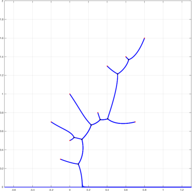
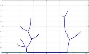
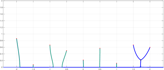
Figure 6: Various examples of solutions of the Problem B.1.

Remark B.3 (Bound on the genus of the surface)

The maximum genus of the double cover associated to the Zakharov–Shabat quadratic differential in this case coincides with the case when, for appropriate configurations, we have a unique double zero of $Q$ on ${\mathbb{R}}$ and all other simple zeros in ${{\mathbb{H}}}$; a count in this case shows that there are a maximum of $2N+2N-2$ branch-points so that the genus is $2N-2$. See Fig. 6.

References

- [1] E. D. Belokolos, A. I. Bobenko, V. Z. Enolski, A. R. Its, and V. B. Matveev, “Algebro-geometric Approach to Non-linear Integrable Equations”, Springer, New York, 1994.
- [2] M. Bertola, T. Grava, and G. Orsatti, “Soliton shielding of the focusing nonlinear Schrödinger” equation. Phys. Rev. Lett., 130(12):Paper No. 127201, 6, 2023.
- [3] R. Bott, “Morse Theory Indomitable”. Publications Mathématiques de l’IHES (1988). 68: 99–114. doi:10.1007/bf02698544
- [4] G. A. El, “The thermodynamic limit of the Whitham equations”, Phys. Lett. A 311, 374-383 (2003).
- [5] G. A. El, “Soliton gas in integrable dispersive hydrodynamics”, J. Stat. Mech.: Theor. Exp., 114001, (2021)
- [6] G.A. El and A. Tovbis, “Spectral theory of soliton and breather gases for the focusing nonlinear Schrödinger equation”, Phys. Rev. E 101, 052207 (2020).
- [7] M. G. Forest and J.-E. Lee, “Geometry and modulation theory for the periodic Nonlinear Schrödinger equation”, in Oscillation Theory, Computation, and Methods of Compensated Compactness, edited by C. Dafermos, J. L. Ericksen, D. Kinderlehrer, and M. Slemrod (Springer New York, New York, NY, 1986) pp. 35–70
- [8] M. Girotti, T. Grava, R. Jenkins, K. McLaughlin, and A. Minakov. “Soliton versus the gas: Fredholm determinants, analysis, and the rapid oscillations behind the kinetic equation”, Comm. Pure and Appl. Math., 76.11 (2023), pp. 3233–3299. doi: 10.1002/cpa.22106
- [9] G. M. Goluzin, “Geometric theory of functions of a complex variable”, Transl. Math. Monogr., Vol. 26 American Mathematical Society, Providence, RI, 1969. vi+676 pp.
- [10] H. Grötzsch,“Über die Verzerrung bei schlichten nichtkonformen Abbildungen und übereine damit zusamenhängende Erweiterung des Picardschen Satzes”. Ber. Verh. Sächs. Akad. Wiss. Leipz., Math.-Phys. Kl. 80 (1928), 503-507.
- [11] S. Grushevsky, I. M. Krichever and C. Norton, “Real-normalized differentials: limits on stable curves”, Russ. Math. Surv., 74, 265, DOI 10.1070/RM9877 (2019)
- [12] A.R.Its and V.P.Kotlyarov, “Explicit formulas for solutions of the Schr’́odinger nonlinear equation”,cDoklady Akad.Nauk Ukrainian SSR, ser.A, no.10, 1976, 965-968.
- [13] J. A. Jenkins, “Univalent functions and conformal mapping”. Reihe: Moderne Funktionentheorie. Springer-Verlag, Berlin-Göttingen-Heidelberg, 1958. Ergebnisse der Mathematik und ihrer Grenzgebiete, (N.F.), Heft 18.
- [14] J. A. Jenkins, “On certain problems of minimal capacity”. Illinois J. Math., 10:460–465, 1966.
- [15] J. A. Jenkins and D. C. Spencer. Hyperelliptic trajectories. Ann. of Math. (2), 53:4–35, 1951.
- [16] R. Jenkins and A. Tovbis, “Approximation of the thermodynamic limit of finite-gap solutions of the focusing NLS hierarchy by multisoliton solutions”, submitted (arXiv:2408.13700).
- [17] A. Kuijlaars and A. Tovbis, “On minimal energy solutions to certain classes of integral equations related to soliton gases for integrable systems”, Nonlinearity 34 no. 10 7227 (2021) (arXiv:2101.03964)
- [18] G. V. Kuzmina, “The general coefficient theorem of Jenkins and the method of modules of curve families”, J. Math. Sci (N.Y.) 207 (2015) no. 6, 898–908.
- [19] G. V. Kuzmina, “On the existence of quadratic differentials with poles of higher orders”, J. Math. Sci. (New York) 83 (1997), no. 6, 772-778.
- [20] G. V. Kuzmina, “On the existence of quadratic differentials with prescribed properties”, J. Math. Sci. (New York) 89 (1998), no. 1, 996-1007.
- [21] Lavrentieff, M, “Sur un problème de maximum dans la représentation conforme”,C. R., 191, (1930), 827–829.
- [22] Lavrentieff, M, “On the theory of conformal mappings”, Trudy Fiz.-Mat. Inst. Steklov. Otdel. Mat., 5, (1934), 159–245 (Russian)
- [23] A. Martinez-Finkelshtein and E. A. Rakhmanov, “Critical measures, quadratic differentials,and weak limits of zeros of Stieltjes polynomials”, Comm. Math. Phys., 302 (2011), no. 1, 53-111.
- [24] J. Milnor, “Morse theory”, Annals of Mathematics Studies, no. 51, Princeton University Press, Princeton, NJ, 1963.
- [25] R. Nevanlinna, “Uniformisierung” Springer, 1953.
- [26] Christian Pommerenke. Univalent functions, volume Band XXV of Studia Mathematica/Mathematische Lehrbücher [Studia Mathematica/Mathematical Textbooks]. Vandenhoeck Ruprecht, Göttingen, 1975. With a chapter on quadratic differentials by Gerd Jensen.
- [27] E. A. Rakhmanov, “Orthogonal polynomials and S-curves”, Contemp. Math., 578, Amer.Math. Soc., Providence, RI, 2012.
- [28] E.B. Saff and V. Totik, Logarithmic Potentials with External Fields, Springer Verlag, Berlin, 1997.
- [29] M. Schiffer and D. Spencer, Functionals of finite Riemann surfaces, Princeton University Press, Princeton, N. J., 1954.
- [30] H. Stahl, Extremal domains associated with an analytic function. I, II, Complex Variables Theory Appl. 4 (1985), no. 4, 311-324, 325-338.
- [31] K. Strebel, “Quadratic differentials”, volume 5 of Ergebnisse der Mathematik und ihrer Grenzgebiete (3) [Results in Mathematics and Related Areas (3)]. Springer-Verlag, Berlin, 1984.
- [32] A. Tovbis and F. Wang, Recent developments in spectral theory of the focusing NLS soliton and breather gases: the thermodynamic limit of average densities, fluxes and certain meromorphic differentials; periodic gases, J. Phys. A: Math. Theor. 55, 424006 (2022).
- [33] A. Tovbis and F. Wang, “Soliton condensates for the focusing Nonlinear Schrodinger Equation: a non-bound state case”, SIGMA 20 (2024), 070, 26p (arXiv 2312.16406)
- [34] S. Venakides, “The continuum limit of theta functions”, Commun. Pure Appl. Math. 42 , (1989), 711-728
- [35] A. Vincent, A. Papadopoulos, “A commentary on Teichmüller’s paper Vollständige Lösung einer Extremalaufgabe der quasikonformen Abbildung” IRMA Lect. Math. Theor. Phys., 27 European Mathematical Society (EMS), Zürich, 2016, 561-567.
- [36] V. E. Zakharov, “Kinetic equation for solitons”, Sov. Phys. JETP, 33, 538 (1971).