appendixOnline Appendix References

Wang, Zhang, Zhang

Large Language Models for Market Research

Large Language Models for Market Research:
A Data-augmentation Approach

Mengxin Wang¹, Dennis J. Zhang², Heng Zhang^{3 1}Naveen Jindal School of Management, The University of Texas at Dallas, Richardson, Texas 75080
²Olin School of Business, Washington University in St. Louis, St. Louis, MO 63130
³W. P. Carey School of Business, Arizona State University, Phoenix, AZ 85069
mengxin.wang@utdallas.edu, denniszhang@wustl.edu, hzhan388@asu.edu

TBD

Large Language Models (LLMs) have transformed artificial intelligence by excelling in complex natural language processing tasks. Their ability to generate human-like text has opened new possibilities for market research, particularly in conjoint analysis, where understanding consumer preferences is essential but often resource-intensive. Traditional survey-based methods face limitations in scalability and cost, making LLM-generated data a promising alternative. However, while LLMs have the potential to simulate real consumer behavior, recent studies highlight a significant gap between LLM-generated and human data, with biases introduced when substituting between the two. In this paper, we address this gap by proposing a novel statistical data augmentation approach that efficiently integrates LLM-generated data with real data in conjoint analysis. Our method leverages transfer learning principles to debias the LLM-generated data using a small amount of human data. This results in statistically robust estimators with consistent and asymptotically normal properties, in contrast to naive approaches that simply substitute human data with LLM-generated data, which can exacerbate bias. We validate our framework through an empirical study on COVID-19 vaccine preferences, demonstrating its superior ability to reduce estimation error and save data and costs by 24.9% to 79.8%. In contrast, naive approaches fail to save data due to the inherent biases in LLM-generated data compared to human data. Another empirical study on sports car choices validates the robustness of our results. Our findings suggest that while LLM-generated data is not a direct substitute for human responses, it can serve as a valuable complement when used within a robust statistical framework.

Conjoint Analysis; Data Augmentation; Large Language Models

1 Introduction

Large Language Models (LLMs) have revolutionized artificial intelligence (AI) by delivering unprecedented capabilities in natural language processing. These models are built on advanced deep learning architectures known as transformer networks, which excel at handling sequential data and understanding context (Vaswani 2017, Radford 2018). Trained on extensive and diverse datasets—including vast amounts of text from books, articles, and websites—LLMs are capable of generating human-like responses and performing complex language tasks. For example, Llama 3 was trained on 15 trillion tokens of data (HuggingFace 2024). This training enables LLMs to comprehend and produce coherent, contextually relevant text, making them invaluable tools in a wide range of applications (Brown 2020).

The rapid development of LLMs also signifies a transformative moment in the social sciences. In market research—a critical area in marketing science and operations management—understanding market demand for products or services is paramount. Traditional market research methods, such as surveys, focus groups, and conjoint analysis, often require significant resources and time. Gathering data from real subjects involves designing intricate questionnaires, recruiting participants, and analyzing responses, all of which can be both costly and logistically challenging (Hair Jr et al. 2019). LLMs present a novel solution by enabling the generation of synthetic data that simulates real consumer behavior without the need for extensive fieldwork. This potential has sparked growing interest among researchers. Thus, a key advantage of using LLMs in market research is their ability to scale data generation: whereas raditional methods often limit the volume of data that can be feasibly collected due to constraints on time and resources, LLMs can rapidly generate large volumes of data, facilitating more comprehensive and granular analysis.

LLMs are trained on vast amounts of data from diverse sources across the internet, including reviews, purchase decisions, and even real survey data on products and services from various categories. The underlying assumption, expressed with some exaggeration, is that LLMs have been exposed to everything there is to see. Researchers hypothesize that the responses LLMs generate for market research surveys could, to some extent, reflect the types of responses that real consumers—represented in the training data—would have given to the same questions. These factors suggest that LLMs may become invaluable tools for gaining insights into consumer preferences, thanks to their ability to mimic or replicate human responses (Brand et al. 2023). Recent studies provide encouraging evidence supporting this potential (Argyle et al. 2023, Chen et al. 2023, Horton 2023). For instance, research shows that by fine-tuning a model (Gururangan et al. 2020) or employing prompting techniques such as chain-of-thought (CoT) reasoning (Brown 2020), it is possible to generate simulated responses in market surveys that resemble those of real human subjects (Brand et al. 2023, Goli and Singh 2024). These explorations suggest the enormous potential of LLMs for advancing market research.

Nonetheless, recent literature also highlights several caveats. Despite some encouraging findings by Goli and Singh (2024), the authors acknowledge that even the most up-to-date prompt engineering methods and advanced LLMs, such as GPT-4 from OpenAI, cannot completely eliminate discrepancies between human and LLM responses in market surveys. For example, they observe that GPT-4 exhibits a pronounced level of impatience compared to human participants. This led the authors to conclude that “directly eliciting preferences using LLMs can yield misleading results,” suggesting that LLMs should be used more as tools to facilitate hypothesis exploration rather than as direct substitutes for human responses. Similarly, Gui and Toubia (2023) points out that LLMs tend to make unintended assumptions about unspecified details of the choice environment, further complicating their use in market research.

We acknowledge the significant potential of LLM-generated labels for market research, but we also believe that the aforementioned gap is likely to persist, even with the most advanced future developments in AI. Consider conjoint analysis, which is arguably the most fundamental methodology for understanding consumer preferences and decision-making processes in market research (Green and Srinivasan 1990). Typically, the researcher seeks to understand how consumers value different features or attributes of a product or service (for details on the setup, please refer to Section 3). At its core, customers aim to maximize their benefits by selecting the optimal products based on their past experiences. However, we emphasize that LLMs do not possess real-life experiences. Additionally, consumer preferences evolve over time due to trends, technological advancements, and economic and cultural shifts (Solomon 2020), changes that LLMs may not accurately capture.

The gap between an LLM’s predictions and actual customer preferences can lead to misleading results if a researcher simply replaces real data with AI-generated data or naively combines the two—a point underscored in Goli and Singh (2024) through careful empirical studies. This observation aligns with our findings. We conducted an empirical study on the conjoint analysis of COVID-19 vaccine preferences, pooling real data with LLM-generated responses based on the same set of product features and performing the conjoint analysis in a manner similar to Brand et al. (2023) (see Section 5 for details of the study). The results are presented in Figure 1. Regardless of the version of the LLM used or whether state-of-the-art prompting techniques are applied, there is a significant gap between the ground-truth model coefficients and those estimated using pooled data. This gap does not diminish with the inclusion of more LLM-generated data; in most models, it actually worsens as more LLM-generated data is added. In contrast, as one would expect, the gap decreases when more real data is incorporated, eventually vanishing to zero, highlighting a stark contrast with the LLM-generated data.

Figure 1: LLM-generated Data $\neq$ Human Data

Notes:

The plot shows the percentage error of estimation based on pooling the real customer response data and LLM-generated data, $\big{\lVert}{\big{(}\hat{\bm{\beta}}-\bm{\beta}^{*}\big{)}}/{\bm{\beta}^{*}}\big{\rVert}_{1}$, where the ratio is taken component-wise. Different curve corresponds to estimators obtained using different AI-generated or real labels. For more details, please refer to Section 5. The horizontal axis gives the quantity of data pooled into the model.

Recognizing that AI-generated data, while informative, is inherently imperfect and likely to be misleading if used naively, our goal is to develop a scheme for its efficient utilization. Although engineering techniques such as fine-tuning, chain-of-thought prompting, and in-context learning can potentially improve the quality of data from LLMs, our objective is to introduce a statistical approach that can be broadly applied independently of these methods and have theoretical guarantees. Our research question is then: Can we improve conjoint analysis by effectively integrating LLM-generated data with real data to produce more accurate estimators of customer preferences, compared to using human data, LLM-generated data, or a naive combination of both? Our method is inspired by the widely recognized knowledge distillation and transfer learning approach in the deep learning literature (Hinton 2015). By formalizing and adapting its core principles to our context, we present a data-augmentation statistical approach for extracting value from LLM- and AI-generated conjoint data. Specifically, we make the following key contributions.

A theoretical framework for data augmentation. The foundation of our framework combines principles of transfer learning and knowledge distillation. Transfer learning, a broad field in computer science, focuses on transferring knowledge from one domain to another, typically reducing the data requirements in the target domain (Pan and Yang 2009, Zhuang et al. 2020). A common approach is to use embeddings learned from one classification task as inputs for another, leveraging pre-learned representations rather than starting from raw data. In our setting, although the large, complex LLM is pretrained for general purposes, it contains valuable knowledge about customer behavior that can be adapted to conjoint analysis. By effectively transferring this knowledge, we can significantly reduce the amount of human data required to achieve a given accuracy. However, this transfer must be grounded in robust statistical learning procedures.

Our method specifically draws on concepts from the knowledge distillation literature. In knowledge distillation, a student model learns by regularizing its outputs against those of a teacher model, effectively transferring the teacher’s knowledge to the student (Hinton 2015). Inspired by this approach, we observe that while LLM-generated data may be misaligned, this bias can be mitigated with a certain amount of real data. To achieve this, using the real data, we train a “soft-target” model that specifies the conditional probability of observing a real label given product features and the LLM-generated label. This model is trained using the empirical Kullback–Leibler (KL) divergence as the loss, which enables the logistic regression model to mimic these soft targets.

Crucially, our approach departs from naive methods illustrated in Figure 1. Rather than assuming LLM-generated labels are perfect, we combine them with real data to transfer knowledge from the LLM to the logistic regression model. This process aligns with a core principle of transfer learning: modeling the differences between human-generated and LLM-generated data is significantly easier than directly modeling human preferences. We demonstrate that this procedure produces consistent and asymptotically normal estimators—statistical properties unattainable with naive methods when LLM labels are biased. Furthermore, we show that our approach guarantees improvements over using human data alone, LLM-generated data alone, or naive combinations of the two.

Large-scale empirical validation. We further conduct empirical analysis, which provides strong evidence supporting the practical value of our estimation framework with AI-generated labels in augmenting real choice-based conjoint data with LLM-generated labels. Using a real-world COVID-19 vaccination dataset, we demonstrate that our estimator consistently reduces estimation error when compared to naive augmentation approaches, even when GPT-generated labels are imperfect. Notably, our estimator’s ability to regularize errors is robust across different versions of GPT and prompt engineering techniques, with CoT prompting yielding the largest error reductions, especially for GPT-4. Our findings highlight the importance of combining LLM-generated data with real-world datasets to achieve reliable and accurate results. Additionally, the empirical results show substantial data savings by up to 24.9% to 79.8% with our estimation approach, suggesting that it is a cost-effective solution for reducing reliance on expensive, human-generated survey data. Lastly, we quantify the value of LLM-generated labels, demonstrating that the proposed estimator can achieve performance equivalent to datasets with up to 80% correct labels, further validating the utility of AI-augmented data in market research contexts. We conduct another empirical study on sports car choice to validate the robustness of our method.

We briefly discuss the organization of our paper. In Section 2, we present a literature review. In Section 3, we set up our model and formally state our data-augmentation approach. We discuss the theoretical properties of our proposed approach in Section 4 and two empirical studies in Sections 5 and 6. In Section 7, we conclude.

2 Literature

In this section, we review several key streams of literature relevant to our research.

Technical Development of natural language processing (NLP) and LLM. The development of LLMs represents a culmination of decades of advances in NLP and deep learning techniques. The foundational work of Chomsky (1956) introduced formal models for language description, paving the way for computational approaches to linguistic analysis. Modern LLMs owe much to significant technical breakthroughs in recent years, such as the introduction of sequence-to-sequence models (Sutskever 2014) and the Transformer architecture (Vaswani 2017), which enables efficient handling of sequential data and contextual understanding.

Key milestones in this area include the development of BERT (Devlin 2018), which introduced bidirectional context modeling, and GPT (Radford 2018), which leveraged generative pre-training to advance NLP capabilities. These innovations culminated in LLMs like GPT-4 (OpenAI 2023), characterized by their ability to perform complex language tasks after training on massive datasets, such as the 15 trillion tokens used to train Llama 3 (HuggingFace 2024). Importantly, further improvements, such as domain-specific adaptations as effective strategies for fine-tuning (e.g., see Beltagy et al. 2019, Gururangan et al. 2020, Parthasarathy et al. 2024) and few-shot learning (Brown 2020) enable these models to achieve remarkable performance in specific tasks. We refer the readers to Naveed et al. (2023) for a reivew of the broader trajectory of LLM research. These technical advancements underpin the transformative potential of LLMs in applications such as social science and consumer behavior modeling.

Using LLMs for Social Sciences and Market Research. AI, especially LLMs, is making a pronounced impact on social sciences. Researchers have explored how these models can simulate human behavior and provide insights into societal phenomena. For instance, Ziems et al. (2024) discuss the potential of LLMs to transform computational social science by generating synthetic data and modeling complex social dynamics. However, questions remain about the reliability of these models in replicating real-world behavior, as highlighted by Huang et al. (2024) and Yang et al. (2024), who caution against over-reliance on LLMs for social predictions due to their lack of lived experiences and contextual nuances. Similarly, Gui and Toubia (2023) point out challenges in using LLMs to simulate human behavior, especially from a causal inference perspective, where the models may fail to account for underlying causality in decision-making processes.

In the domain of market research, LLMs have emerged as powerful tools for generating synthetic data that mimics human responses. Studies such as Brand et al. (2023) and Argyle et al. (2023) demonstrate the feasibility of using LLMs for simulating consumer preferences, while Chen et al. (2023) and Horton (2023) highlight the potential of these models as simulated economic agents. Still, the extent to which LLMs can faithfully replicate human preferences remains a point of debate, as explored by Goli and Singh (2024), who emphasize the challenges in achieving alignment between AI-generated and human data. Our work provides an alternative perspective on this question: while LLMs may not fully replicate human behavior or replace humans in social sciences or market research, they can nonetheless offer valuable insights to improve existing methods. With the implementation of robust statistical procedures for correcting bias, LLMs can serve as effective tools for enhancing the accuracy and efficiency of current methodologies.

Conjoint Analysis. Conjoint analysis has long been a cornerstone of market research, providing insights into consumer preferences by evaluating trade-offs between product attributes (Green and Srinivasan 1978, 1990). Over time, this methodology has seen significant methodological advancements. In operations, early work by Kohli and Sukumar (1990) and Wang et al. (2009) explored heuristics and optimization approaches for product line design, while Kessels et al. (2008) focused on experimental design for conjoint studies. Recent contributions, such as Dzyabura and Jagabathula (2018), extend conjoint analysis to multi-channel settings, incorporating both online and offline consumer behaviors.

Our research builds on the rich tradition of integrating methods from statistics or machine learning (ML) into conjoint analysis. While prior studies have leveraged advanced statistical models (Allenby and Rossi 2006) and Bayesian frameworks (Eggers et al. 2021), we introduce a novel data augmentation approach that bridges the gap between AI-generated and real-world data. Furthermore, as mentioned, Goli and Singh (2024) emphasize the limitations of using LLM-generated data alone for preference estimation, underscoring the need for innovative solutions like our proposed methodology. This methodological contribution represents a significant step forward in enhancing the robustness and scalability of conjoint analysis.

Technology, Innovation, and Entrepreneurship. Our work also speaks to the literature of technology, innovation, and entrepreneurship, the intersection of which has been a focal point of operations management research. Foundational works such as Shane and Ulrich (2004) provide a comprehensive overview of how technological advancements drive product development and entrepreneurial activities. Recent studies emphasize the role of AI and ML in reshaping operational tasks. For instance, Terwiesch (2019) and Bastani et al. (2022) highlight the potential of AI tools to optimize decision-making processes, while Yoo et al. (2024) identify new frontiers in digital innovation.

Our work contributes to this stream by demonstrating how LLMs represent a disruptive innovation in market research. By democratizing access to market insights, LLMs enable startups and smaller firms to conduct sophisticated analyses previously reserved for resource-intensive operations (Olsen and Tomlin 2020, Choi et al. 2022). Furthermore, our findings align with Girotra et al. (2023), which discusses the transformative role of LLMs in idea generation and business innovation. Along a similar line, Connell and Choi (2024) discusses how to correct the misclassification error in using LLM in place of human for classifying textual data, and Ludwig et al. (2024) develops an econometric framework to assess the validity of using LLMs in economics research, emphasizing the need to avoid training data leakage for prediction tasks and to ensure gold-standard measurement equivalence for estimation tasks, while providing guidance on mitigating potential biases and limitations. Collectively, these insights underscore the potential of new technologies to revolutionize traditional operational practices, particularly for data collection and consumer analysis.

By situating our research within these four streams of literature, we highlight its relevance and contributions to both methodological and practical advancements. Our work not only extends the technical capabilities of conjoint analysis but also demonstrates the broader impact of LLMs as tools for innovation in social sciences and operations management.

3 Model and the Data-augmentation Approach

In this section, we establish the theoretical framework. Although our approach can be extended to various market research settings, we focus on conjoint analysis as the primary use case to present the theory and conduct the empirical analysis detailed in Section 5.

3.1 Setup

In this section, we provide a detailed explanation of the setup, starting with an in-depth discussion of the theoretical framework underlying the data generation process. We will outline the assumptions, structure, and specific parameters that guide this process, building a foundation for understanding how the data is conceptualized and modeled within this framework.

3.1.1 Data Generation Process and the Best-in-class Estimation.

Consider a setting where we observe two datasets. The first, referred to as the primary data, consists of $m$ data points, $\left\{\big{(}\mathbf{x}^{\sf P}_{i},y^{\sf P}_{i},z^{\sf P}_{i}\big{)}\right\}_{i=1}^{m}$. For a fixed positive integer $k$, we denote the set $\{1,\dots,k\}$ by $\mathcal{K}$ and define $\mathcal{K}^{+}=\mathcal{K}\cup\{0\}$. These data points are independently and identically distributed (i.i.d.) according to the same distribution as the random vector $(\mathbf{x},y,z)$, where $y,z\in\mathcal{K}^{+}$ and $\mathbf{x}\in\mathbb{R}^{dk}$. To clarify, in the context of conjoint analysis with AI-generated labels, $\mathbf{x}$ represents the features or context of a choice setting, and $y$ denotes the respondent’s choice. Here, $\mathcal{K}^{+}$ corresponds to the $k+1$ options available to the respondent, where $0$ represents the outside option. Additionally, $\mathbf{x}=(\mathbf{x}^{\top}_{(1)},\mathbf{x}^{\top}_{(2)},\dots,\mathbf{x}^{\top}_{(k)})^{\top}$, where $\mathbf{x}^{\top}_{(j)}$ corresponds to the features of option $j$ for each $j\in\mathcal{K}$. Throughout this paper, we refer to the random variable $y$ as the real label. The variable $z$ represents a predicted label generated by an AI model based on $\mathbf{x}$, and we refer to it as the AI-generated label. The second dataset, called the auxiliary data, consists of $\left\{\big{(}\mathbf{x}_{i},z_{i}\big{)}\right\}_{i=1}^{n}$, which are independent of the primary data but follow the same distribution. However, in the auxiliary data, the true label $y_{i}$ is missing for each data point. In Figure 2, we illustrate this theoretical setup for conjoint analysis using an example simplified from the empirical setting in Section 5.

How is this data generation process implemented in practice? A manager facing a conjoint study problem can begin by collecting a small sample of human response data. Using the same questions presented to human respondents, the manager can query an LLM to generate the primary dataset containing both labels $y$ and $z$. Subsequently, the manager can generate additional responses by querying the LLM with a different set of choices, which forms the auxillary dataset where the true label $y$ is missing. Since the cost of querying an LLM is negligible compared to recruiting human subjects in many cases, the auxiliary dataset is typically much larger than the primary dataset in size.

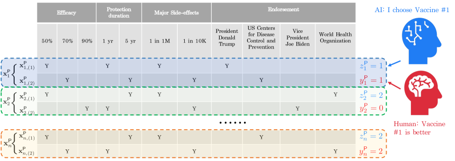
Figure 2: Illustration of the dataset

Notes:

In this figure, we illustrate the primary dataset using an example simplified from the empirical setting in Section 5. For instance, corresponding to the first data point, two vaccine options are presented to the human respondent. The first vaccine has the following features: 50% efficacy, a one-year protection duration, a major side-effect rate of one in a million, a minor side-effect rate of one in ten, and endorsement by President Donald Trump. These features can be converted into a numerical feature vector, $\mathbf{x}^{\sf P}_{1,(1)}$, suitable for conjoint analysis, for example, using one-hot encoding. Based on these features, the AI recommends selecting the first vaccine (i.e., $z^{\sf P}_{1}=1$), which aligns with the human respondent’s choice (i.e., $y^{\sf P}_{1}=1$). Note that the second human respondent opts to select no vaccine from the two offered. The auxiliary dataset is similar to the primary dataset, except that it lacks the human-generated labels for these data points.

We assume that the distribution $\mathbb{P}(y\,|\,\mathbf{x},z)$ can be parameterized as $\mathbb{P}(y=j\,|\,\mathbf{x},z)\,=\,g_{j}(\mathbf{x},z;\bm{\theta}^{*})$ for each $j\in\mathcal{K}^{+}$, where $\bm{\theta}^{*}\in\mathbb{R}^{q}$ is not known to us. This assumption is motivated by the fact that modern artificial AI models, such as an LLM, are trained with vast amounts of text data, including information from numerous sources on the internet, that may contain product reviews, messaging boards, and other online forums with contributions from a wide range of consumers discussing the products they shop for and purchase (Brand et al. 2023). Therefore, AI can “mimic” how respondents make choices, leading to highly informative AI-generated labels. Therefore, the model $\big{(}g_{j}(\mathbf{x},z;\bm{\theta}^{*}):j\in\mathcal{K}^{+}\big{)}$, which can be chosen as the multinomial logit model or a neural network, is specified to capture the conditional probabilities $\mathbb{P}(y\,|\,\mathbf{x},z)$ in practical scenarios. We also assume throughout that $|g_{j}(\cdot)|\leq 1$ for all $j\in\mathcal{K}^{+}$, which is reasonable for a wide range of models.

Consistent with a typical conjoint analysis, our goal is to fit a multinomial logit (MNL) model

$$\sigma_{j}(\mathbf{x};\bm{\beta})~{}=~{}\frac{e^{\mathbf{x}^{\top}_{(j)}\bm{\beta}}}{1+\sum_{\ell\in\mathcal{K}}e^{\mathbf{x}^{\top}_{(\ell)}\bm{\beta}}},~{}~{}\forall\,j\in\mathcal{K},$$ (1)

where the vector $\bm{\beta}\in\mathbb{R}^{d}$ is the coefficient of our interest, to best approximate $\mathbb{P}(y\,|\,x)$. The main goal of the conjoint analysis is to identify the best-in-class estimator—the one that most closely approximates the true choice probabilities within the set of all multinomial logit models. The quality of this approximation is measured by the Kullback–Leibler (KL) divergence. Formally, the best-in-class estimator is defined as follows:

$$\bm{\beta}^{*}~{}\in~{}\argmin_{\bm{\beta}\in\mathbb{R}^{d}}\left\{\mathbb{E}_{\mathbf{x}}\Big{[}{\sf KL}\big{(}\mathbb{P}(y|\mathbf{x})\,\big{|}\,\sigma_{y}(\mathbf{x},\bm{\beta})\big{)}\Big{]}~{}=~{}\mathbb{E}_{\mathbf{x}}\left[\sum_{j\in\mathcal{K}^{+}}\mathbb{P}\big{(}y=j|\mathbf{x}\big{)}\log\left(\frac{\mathbb{P}\big{(}y=j|\mathbf{x}\big{)}}{\sigma_{j}(\mathbf{x};\bm{\beta})}\right)\right]\right\}.$$ (2)

That is, measuring the loss of approximation using the KL-divergence, $\big{(}\sigma_{j}(\mathbf{x};\bm{\beta}^{*}):j\in\mathcal{K}^{+}\big{)}$ gives us the approximate to the true choice probabilities that is best in the class of multinomial logit models. Under reasonable assumptions, this minimizer is uniquely defined (see Theorem 4.3 below).

We further clarify the distinction between our problem and the measurement error issues discussed in the econometrics literature (e.g., see Bound et al. 2001) and in recent work Connell and Choi (2024). Specifically, in our context, $z$ should not be interpreted as a noisy realization of $y$ conditional on $\mathbf{x}$, as is commonly assumed in the measurement error framework. In our setting, $y\perp z\,|\,\mathbf{x}$ because the AI cannot access the internal thought and decision-making processes of a human subject, and any relationship between $y$ and $z$ is mediated entirely through $\mathbf{x}$. Nonetheless, we emphasize that our estimation procedure and theoretical results impose no assumptions on the joint distribution of $y$ and $z$ given $\mathbf{x}$. Therefore, even if $z$ represents $y$ measured with error, our approach remains valid.

3.2 Primary, Auxillary and Naive Estimators

With no access to auxiliary data such as AI-generated labels, the default approach is to fit the parameter $\bm{\beta}$ using only the primary data with its real labels $\left\{\big{(}\mathbf{x}^{\sf P}_{i},y^{\sf P}_{i}\big{)}\right\}_{i=1}^{m}$ using the standard Maximum Likelihood Estimation (MLE). We use $\hat{\bm{\beta}}^{\sf P}$ to denote the estimator obtained using only the primary data. When the primary data size is sufficiently large, $\hat{\bm{\beta}}^{\sf P}$ can be close to $\bm{\beta}^{*}$. However, the size of the primary data is often restricted due to the costs of recruiting real subjects. A small primary set yields a inaccurate estimator that is far away from $\bm{\beta}^{*}$. On the flipping side, we may directly perform MLE on the auxiliary data $\left\{\big{(}\mathbf{x}_{i},z_{i}\big{)}\right\}_{i=1}^{n}$, using $z_{i}$ as labels. Let us define this estimator as $\hat{\bm{\beta}}^{\sf A}$. Given the distribution of LLM-generated data and human data are different (i.e., the distributions of $y$ and $z$, conditioned on $\mathbf{x}$, are different), it is easy to recognize that $\hat{\bm{\beta}}^{\sf A}$ could be severly biased regardless of the size of auxillary dataset compared to $\bm{\beta}^{*}$.

Due to this limitation, people intend to utilize auxiliary data and AI-generated labels to facilitate the estimation of $\bm{\beta}^{*}$. A natural idea for utilizing the AI labels is to simply pool the primary and auxiliary sets. In particular, we define

$$(\tilde{\mathbf{x}}_{i},\tilde{y}_{i})~{}=~{}\begin{cases}({\mathbf{x}}_{i}^{\sf P},y_{i}^{\sf P})~{}&\text{if }1\leq i\leq m\\ ({\mathbf{x}}_{i-m},z_{i-m})~{}&\text{if }m+1\leq i\leq m+n\end{cases},$$

and perform the standard MLE on $(\tilde{\mathbf{x}}_{i},\tilde{y}_{i})_{i=1}^{m+n}$. We call this approach the naïve augmentation and write the estimator as $\hat{\bm{\beta}}^{\sf Naive}$. The auxiliary data largely enlarges the data size. However, since $z$ and $y$ come from different distributions, $\hat{\bm{\beta}}^{\sf Naive}$ will be biased, even with large data size. Note that both $\hat{\bm{\beta}}^{\sf P}$ and $\hat{\bm{\beta}}^{\sf A}$ are both special cases of $\hat{\bm{\beta}}^{\sf Naive}$ by setting $n=0$ or $m=0$. In the following, we present a simple example to demonstrate the limitations of these estimators discussed above and generalize the observation in Proposition 3.2.

Example 3.1 (AI-Generated Data Cannot Replace Human Data)

Consider a simple setting with only one product and no features. AI-generated label are very close to human label: Conditional on $z=j$, where $j\in\mathcal{K}^{+}=\{0,1\}$, $y=j$ with probability $p$. Suppose that $\mathbb{P}(z=1)=\alpha$. Therefore, the probability that $y=1$ is given by $\alpha p+(1-\alpha)(1-p)$ and clearly the best-in-class estimator in (1) is given by $\beta^{*}=1+\log(\alpha p+(1-\alpha)(1-p))$, which satisfies

$$\mathbb{P}(j=1)~{}=~{}\alpha p+(1-\alpha)(1-p)~{}=~{}\frac{e^{\beta^{*}}}{1+e^{\beta^{*}}}.$$

Suppose that $n/m=\rho\neq 0$. Then naive estimator satisfies

$$\frac{\alpha\rho}{1+\rho}+\frac{\alpha p+(1-\alpha)(1-p)}{1+\rho}~{}=~{}\frac{e^{\hat{\beta}^{\sf Naive}}}{1+e^{\hat{\beta}^{\sf Naive}}},$$

which leads to

$$\hat{\beta}^{\sf Naive}~{}=~{}1+\log\left(\frac{\alpha\rho}{1+\rho}+\frac{\alpha p+(1-\alpha)(1-p)}{1+\rho}\right).$$

Unless $\alpha=1/2$ or $p=1$, $\hat{\beta}^{\sf Naive}\neq\beta^{*}$. This is always the case even when $n,m\rightarrow\infty$, as long as $\rho\neq 0$. We also note that when $p$ is close to one, $z$ is very informative of $y$ but the naïve methods still cannot lead to desired estimates. $\blacksquare$

Proposition 3.2 (Bias of $\hat{\bm{\beta}}^{\sf A}$ and $\hat{\bm{\beta}}^{\sf Naive}$.)

$\hat{\bm{\beta}}^{\sf A}$ and $\hat{\bm{\beta}}^{\sf Naive}$ are generally biased even for $m,n\rightarrow\infty$.

3.3 Estimation with AI-augmented Data

These challenges lead to our research question: How do we extract value from the AI-augmented data to facilitate the estimation of $\bm{\beta}^{*}$? To answer this question, we propose the following data augmentation approach that allows us to use the AI-generated data to fit the model.

Estimation with AI-Augmented Data:

 

Step 1. Obtain an estimator $\hat{\bm{\theta}}$ to $\bm{\theta}^{*}$, where $\mathbb{P}(y=j\,|\,\mathbf{x},z)\,=\,g_{j}(\mathbf{x},z;\bm{\theta}^{*})$, using the primary data.

Step 2. With the auxiliary data, we construct the estimator $\hat{\bm{\beta}}^{\sf AAE}$ as

$$\hat{\bm{\beta}}^{\sf AAE}~{}=~{}\argmax_{\bm{\beta}\in\mathbb{R}^{d}}\,\left\{\widehat{Q}(\hat{\bm{\theta}};\bm{\beta})\,=\,\frac{1}{n}\sum_{i=1}^{n}\sum_{j\in\mathcal{K}^{+}}g_{j}(\mathbf{x}_{i},z_{i};\hat{\bm{\theta}})\log\sigma_{j}(\mathbf{x};\bm{\beta})\right\}.$$

 

We refer to $\hat{\bm{\beta}}^{\sf AAE}$ as the AI-augmented estimator (AAE). In the next section, we demonstrate that our estimator $\hat{\bm{\beta}}^{\sf AAE}$ successfully recovers $\bm{\beta}^{*}$ and exhibits the desired asymptotic properties. The key idea in our approach is to use the primary dataset—which contains both LLM-generated and human-produced data—to learn an efficient mapping between huamn and LLM-generated data. We then leverage this mapping when combining the primary and auxiliary datasets. This strategy closely resembles a transfer learning approach, where knowledge from one domain (in our case, the LLM-generated data) is transferred to another domain (the human-produced data). The fundamental assumption underpinning such transfer learning techniques is that learning the mapping function between two domains, denoted by $g(\cdot)$ in our context, is inherently simpler and requires fewer data points than carrying out the individual learning tasks within either domain on its own. In other words, in our context, the AI model undertakes the “heavy lifting” of capturing human choice behavior in a fuzzing way, and the first-stage in our estimation is trying to capture how fuzzy this AI model is compared to the human model. Moreover, the mapping will become easier to learn with lower LLM costs and higher LLM quality. This is because, as the accuracy and the size of AI-generated labels improves, we anticipate a high-quality estimation of $\bm{\theta}$ due to a decrease in the asymptotic variance of $\bm{\theta}$ estimation; see Section 4.2 for further discussion.

4 Theoretical Properties of Our Estimator

In this section we provide a theoretical analysis of our estimator, $\hat{\bm{\beta}}^{\sf AAE}$. In Section 4.1, we present the main theoretical results, i.e., the consistency and asymptotic normality of the estimator. We then discuss the efficiency gain by using our estimator compared to only using human data.

4.1 Main Theoretical Results

To deliver the analysis, a set of common regularity assumptions are needed. Note that these assumptions are typically assumed in asymptotic statistical analysis  (Newey and McFadden 1994, Van der Vaart 2000). The first set of assumptions are used in the analysis of the consistency of $\hat{\bm{\beta}}^{\sf AAE}$.

Assumption 4.1 (Regularity Conditions for Consistency)

The following assumptions hold.

• We assume that $\mathbf{x}\in\mathcal{X}$ with probability one, where $\mathcal{X}$ is bounded. Also, $\mathbb{E}_{\mathbf{x}}[\mathbf{x}\mathbf{x}^{\top}]\succ 0$ and $\mathbb{P}(y\,|\,\mathbf{x})\geq c$ for all $\mathbf{x}\in\mathcal{X}$, $y\in\mathcal{K}$ and some constant $c>0$.

• $\hat{\bm{\theta}}\overset{\text{{P}}}{\rightarrow}\bm{\theta}^{*}$.

• $\big{(}g_{j}(\mathbf{x},z;\bm{\theta}):j\in\mathcal{K}^{+}\big{)}$ is continuous in $\bm{\theta}$ for all $\mathbf{x}\in\mathcal{X}$ and $z\in\mathcal{K}^{+}$.

Comparing to those assumptions required in classical consistency results, such as Theorem 5.1 in Van der Vaart (2000) or Theorem 2.1 in Newey and McFadden (1994), Assumption 4.1 presents similar or even weaker regularity conditions that guarantee consistency in a setting that significantly extends that of classical analysis of MLE under the multinomial logit model, by exploiting the concavity in the problem structure. Part $(i)$ in Assumption 4.1 essentially serves as an identification condition, which should be satisfied in practical scenarios. Part $(ii)$ states that the first-step estimator needs to be consistent, which should be satisfied as long as the models $\big{(}g_{j}(\mathbf{x},z;\bm{\theta}^{*}):j\in\mathcal{K}^{+}\big{)}$ are appropriately specified. Part $(iii)$ is a regularity condition on the functional smoothness. This particular assumption, in principle, can be replaced by weaker one but directly assuming continuity leads to the ease of proof. This assumption holds for many widely used models, for example, the MNL model or the neural networks.

In the next, the second set of assumptions helps establish the asymptotic normality.

Assumption 4.2 (Regularity Conditions for Asymptoical Nomrality)

We assume that the following conditions hold.

• $\sqrt{m}(\hat{\bm{\theta}}-\bm{\theta}^{*})\rightsquigarrow N(\bm{0},\bm{\Lambda})$.

• $\frac{n}{m}\rightarrow\rho$, where $0<\rho<\infty$.

• For each $j\in\mathcal{N}$, there exists a neighborhood $\mathcal{N}$ of $\bm{\theta}^{*}$ such that $\,\mathbb{E}_{\mathbf{x},z}\big{[}\sup_{\bm{\theta}\subset\mathcal{N}}\lVert\nabla_{\bm{\theta}}g_{j}(\mathbf{x},z,\bm{\theta})\rVert_{2}\big{]}\,<\,\infty$ and $g_{j}(\mathbf{x},z,\bm{\theta})$ is continuous at $\bm{\theta}^{0}$ for all $\mathbf{x}\in\mathcal{X}$ and $z\in\mathcal{K}$

The requirements imposed in Assumption 4.2 are again mild. The first item states $\hat{\bm{\theta}}$ is asymptotically normal, which is expected. The second item maintains that the ratio between the sample sizes of two data sets needs to be reasonable. The last item is a smoothness condition. Furthermore, to simplify the presentation, some definitions are necessary. We first define $\mathbf{A}(\mathbf{x};\bm{\beta})\in\mathbb{R}^{k\times k}$ with

$$\mathbf{A}(\mathbf{x};\bm{\beta})~{}:=~{}\sum_{j\in\mathcal{K}}\sigma_{j}(\mathbf{x};\bm{\beta}^{*})\left(\mathbf{x}_{(j)}\mathbf{x}_{(j)}^{\top}-\sum_{j^{\prime}\in\mathcal{K}}\sigma_{j^{\prime}}(\mathbf{x};\bm{\beta})\mathbf{x}_{(j)}\mathbf{x}_{(j^{\prime})}^{\top}\right)$$ (3)

and $\bm{\Omega}\in\mathbb{R}^{k\times k}$ and $\bm{\Gamma}\in\in\mathbb{R}^{k\times q}$ with

$$\bm{\Omega}:=\mathbb{E}_{\mathbf{x}}\left[\mathbf{A}(\mathbf{x};\bm{\beta}^{*})\right]~{}\text{ and }~{}\bm{\Gamma}:=\mathbb{E}_{\mathbf{x},z}\left[\sum_{j\in\mathcal{K}^{+}}\left(\mathbbm{1}_{\{j\neq 0\}}\mathbf{x}_{(j)}-\sum_{j^{\prime}\in\mathcal{K}}\sigma_{j^{\prime}}(\mathbf{x},\bm{\beta}^{*})\mathbf{x}_{(j^{\prime})}\right)\nabla_{\bm{\theta}}g_{j}(\mathbf{x},z,\bm{\theta}^{*})\right].$$ (4)

Also, we let $\mathbf{p}(\mathbf{x},z)\in\mathbb{R}^{k}$ be such that its $j$-th component is $\mathbb{P}(y=j\,|\,\mathbf{x},z)$ and $\bm{\sigma}(\mathbf{x},\bm{\beta}^{*})\in\mathbb{R}^{k}$ be the vector such that its $j$-th component is $\sigma_{j}(\mathbf{x},\bm{\beta}^{*})$. Then,

$$\mathbf{J}~{}=~{}\mathbb{E}_{\mathbf{x},z}\left[\left(\sum_{j\in\mathcal{K}}\big{(}g_{j}(\mathbf{x},z;{\bm{\theta}}^{*})-\sigma_{j}(\mathbf{x};\bm{\beta}^{*})\big{)}\mathbf{x}_{(j)}\right)\left(\sum_{j\in\mathcal{K}}\big{(}g_{j}(\mathbf{x},z;{\bm{\theta}}^{*})-\sigma_{j}(\mathbf{x};\bm{\beta}^{*})\big{)}\mathbf{x}_{(j)}\right)^{\top}\right]\in\mathbb{R}^{k\times k}.$$

Equipped with these assumptions and defintions, we show the following key result.

Theorem 4.3 (Consistency and Asymptotic Normality of AI-augmented Estimator)

• Under Assumption 4.1, the optimizer $\bm{\beta}^{*}$ defined in (2) is unique and the AAE satisfies $\hat{\bm{\beta}}^{\sf AAE}\overset{\text{{P}}}{\rightarrow}\bm{\beta}^{*}$, when $m,n\rightarrow\infty$.

• Under Assumptions 4.1 and 4.2, it holds that

  $$\sqrt{n}(\hat{\bm{\beta}}^{\sf AAE}-\bm{\beta}^{*})~{} =~{}\bm{\Omega}^{-1}\times\left(\frac{1}{n}\sum_{i=1}^{n}\left(\mathbf{p}(\mathbf{x}_{i},z_{i})-\bm{\sigma}(\mathbf{x}_{i},\bm{\beta}^{*})\right)\otimes\mathbf{x}_{i}+\sqrt{\frac{n}{m}}\bm{\Gamma}\times\sqrt{m}(\hat{\bm{\theta}}-\bm{\theta}^{*})\right)+o_{\text{{P}}}(1)$$

  $$\rightsquigarrow~{}N\Big{(}\bm{0},\,\bm{\Omega}^{-1}\big{(}\mathbf{J}+\rho\times\bm{\Gamma}\bm{\Lambda}\bm{\Gamma}^{\top}\big{)}\bm{\Omega}^{-1}\Big{)}.$$

While some aspects of our proof of Theorem 4.3 draw on classical analysis of extremum estimators, the consistency argument we present for a misspecified model with two-stage estimators appears to be novel. First, the identification of the model parameter and its justification (Lemma 4.5) is, to the best of our knowledge, new. Second, with the presence of auxiliary data $z$, we reformulate the loss function as shown in (2). This leads to a novel approach that converts the consistency of $\hat{\bm{\theta}}$ into the uniform convergence of $\widehat{Q}(\hat{\bm{\theta}};\bm{\beta})$ (Lemma 4.6). Third, our consistency analysis, based on concavity also seems fresh.

4.2 Value of AI-Augmented Estimation

We compare our proposed estimator, $\hat{\bm{\beta}}^{\sf AAE}$, with the three benchmark approaches $\hat{\bm{\beta}}^{\sf Naive}$, $\hat{\bm{\beta}}^{\sf A}$ and $\hat{\bm{\beta}}^{\sf P}$ that were discussed in Section 3.2. With Theorem 4.3 and Proposition 3.2, the merit of $\hat{\bm{\beta}}^{\sf AAE}$ over $\hat{\bm{\beta}}^{\sf Naive}$ and $\hat{\bm{\beta}}^{\sf A}$ is clear: while $\hat{\bm{\beta}}^{\sf AAE}$ delivers asymptotically unbiased estimation, both $\hat{\bm{\beta}}^{\sf Naive}$ and $\hat{\bm{\beta}}^{\sf A}$ are in general biased. Thus, the use of $\hat{\bm{\beta}}^{\sf AAE}$ enables valid estimation, inference, or subsequent downstream optimization, for example, for product design, while the other two estimators lead to inferior decisions. Thus, let us focus on the comparison of $\hat{\bm{\beta}}^{\sf AAE}$ and $\hat{\bm{\beta}}^{\sf P}$ to demonstrate that the convergence speed of $\hat{\bm{\beta}}^{\sf AAE}$ being faster than that of $\hat{\bm{\beta}}^{\sf P}$.

In this case, standard analysis shows that, under appropriate regularity conditions, the resulting estimator $\hat{\bm{\beta}}^{\sf P}$ satisfies: $\sqrt{m}\big{(}\hat{\bm{\beta}}^{\sf P}-\bm{\beta}^{*}\big{)}\rightsquigarrow N\Big{(}\bm{0},\,\bm{\Omega}^{-1}\check{\mathbf{J}}\bm{\Omega}^{-1}\Big{)},$ where $\bm{\Omega}$ is defined in (4), and

$$\check{\mathbf{J}}~{}:=~{}\mathbb{E}_{\mathbf{x},y,z}\left[\left(\sum_{j\in\mathcal{K}}\big{(}\mathbbm{1}_{\{y=j\}}-\sigma_{j}(\mathbf{x};\bm{\beta}^{*})\big{)}\mathbf{x}_{(j)}\right)\left(\sum_{j\in\mathcal{K}}\big{(}\mathbbm{1}_{\{y=j\}}-\sigma_{j}(\mathbf{x};\bm{\beta}^{*})\big{)}\mathbf{x}_{(j)}\right)^{\top}\right]\in\mathbb{R}^{k\times k}.$$

By Theorem 4.3, the variance of the AAE, $\hat{\bm{\beta}}^{\sf AAE}$ can be expressed as $\bm{\Omega}^{-1}\mathbf{J}\bm{\Omega}^{-1}/n+\bm{\Omega}^{-1}\bm{\Gamma}\bm{\Lambda}\bm{\Gamma}^{\top}\bm{\Omega}^{-1}/m.$ Thus, our AAE performs better if and only if:

$${\sf Var}^{\sf P}~{}:=~{}\frac{1}{m}\bm{\Omega}^{-1}\check{\mathbf{J}}\bm{\Omega}^{-1}~{}\succeq~{}{\sf Var}^{\sf AAE}~{}:=~{}\frac{1}{n}\bm{\Omega}^{-1}\mathbf{J}\bm{\Omega}^{-1}+\frac{1}{m}\bm{\Omega}^{-1}\bm{\Gamma}\bm{\Lambda}\bm{\Gamma}^{\top}\bm{\Omega}^{-1},$$ (5)

or equivalently $\check{\mathbf{J}}/m\succeq{\mathbf{J}}/n+\bm{\Omega}^{-1}\bm{\Gamma}\bm{\Lambda}\bm{\Gamma}^{\top}/m$. The next result follows.

Proposition 4.4 (Dominance of ${\sf Var}^{\sf AAE}$.)

Assume Assumptions 4.1 and 4.2 hold and

$$\bm{\Lambda}~{}=~{}\mathbb{E}_{\mathbf{x},y,z}\big{[}\nabla_{\theta}\log g_{y}(\mathbf{x},z,\bm{\theta}^{*})\nabla_{\theta}\log g_{y}(\mathbf{x},z,\bm{\theta}^{*})^{\top}\big{]}^{-1}.$$

• It holds that $\check{\mathbf{J}}\succeq\bm{\Gamma}\bm{\Lambda}\bm{\Gamma}^{\top}$. Therefore, for any $\delta>0$ and any $m$, ${\sf Var}^{\sf AAE}\prec{\sf Var}^{\sf P}+\delta\mathbf{I}$ for all $n$ sufficiently large.

• If $\check{\mathbf{J}}\succ\bm{\Gamma}\bm{\Lambda}\bm{\Gamma}^{\top}$, for any $m$, ${\sf Var}^{\sf AAE}\prec{\sf Var}^{\sf P}$ for all $n$ sufficiently large.

Note that the assumption we introduce regarding the form of $\bm{\Lambda}$ is quite mild—it holds as long as $\hat{\bm{\theta}}$ is estimated via maximum likelihood estimation and the standard regularity conditions are met (Van der Vaart 2000). The first part of the proposition asserts that the variance of AAE weakly dominates the variance of $\hat{\bm{\beta}}^{\sf P}$: as long as the auxiliary dataset is sufficiently large, the variance of $\hat{\bm{\beta}}^{\sf AAE}$ does not exceed that of $\hat{\bm{\beta}}^{\sf P}$, up to an arbitrarily small constant. This conclusion follows directly since $\check{\mathbf{J}}\succeq\bm{\Gamma}\bm{\Lambda}\bm{\Gamma}^{\top}$ and we can let $n$ tend toward infinity. The argument hinges on representing $\check{\mathbf{J}}-\bm{\Gamma}\bm{\Lambda}\bm{\Gamma}^{\top}$ as the variance of the residual from projecting $\sum_{j\in\mathcal{K}}\big{(}\mathbbm{1}_{\{y=j\}}-\sigma_{j}(\mathbf{x};\bm{\beta}^{*})\big{)}\mathbf{x}_{(j)}$ onto the linear space spanned by $\nabla_{\theta}\log g_{y}(\mathbf{x},z,\bm{\theta}^{*})$. For the second part, if $\check{\mathbf{J}}\succ\bm{\Gamma}\bm{\Lambda}\bm{\Gamma}^{\top}$, the strong dominance ${\sf Var}^{\sf AAE}\prec{\sf Var}^{\sf P}$ for all sufficiently large $n$ follows by a similar reasoning.

Is $\check{\mathbf{J}}\succ\bm{\Gamma}\bm{\Lambda}\bm{\Gamma}^{\top}$ generally true? By interpreting $\check{\mathbf{J}}-\bm{\Gamma}\bm{\Lambda}\bm{\Gamma}^{\top}$ as the variance of the residual from projecting $\sum_{j\in\mathcal{K}}\big{(}\mathbbm{1}_{\{y=j\}}-\sigma_{j}(\mathbf{x};\bm{\beta}^{*})\big{)}\mathbf{x}_{(j)}$ onto the space spanned by $\nabla_{\theta}\log g_{y}(\mathbf{x},z,\bm{\theta}^{*})$, we observe that this inequality should hold in many cases, although providing a general, primitive sufficient condition seems challenging without a specific form of $g(\cdot)$. To illustrate this further and gain more insights, we refer the readers to Appendix 9, where we show that under specific parametric forms of $g(\cdot)$, item (ii) in the proposition indeed holds in general.

4.3 Proof Sketch of Theorem 4.3

In this section, we sketch the arguments leading to Theorem 4.3. Some technical arguments are deferred to the appendix.

4.3.1 Proof of the First Part of Theorem 4.3.

As the first step, we argue that the optimizer in (2) is uniquely defined, whose proof we defer to the appendix. This result only requires $(i)$ in Assumption 4.1.

Lemma 4.5 (Unique Optimizer)

There exists an unique optimizer in (2).

Given the lemma, we can link the global loss function to the empirical loss function that we use as follows. By Lemma 4.5, $\bm{\beta}^{*}$ is the unique solution to $\max_{\bm{\beta}\in\mathbb{R}^{k}}Q(\bm{\beta})$, where

$$Q(\bm{\beta})~{}:=~{} \mathbb{E}_{\mathbf{x}}\left[\sum_{j\in\mathcal{K}^{+}}\mathbb{P}\big{(}y=j|\mathbf{x}\big{)}\log\sigma_{j}(\mathbf{x},\bm{\beta})\right]~{}\stackrel{{\scriptstyle\text{(a)}}}{{=}}~{}\mathbb{E}_{\mathbf{x}}\left[\sum_{j\in\mathcal{K}^{+}}\mathbb{E}_{z}\big{[}\mathbb{P}\big{(}y=j|\mathbf{x},z\big{)}\big{|}\mathbf{x}\big{]}\log\sigma_{j}(\mathbf{x},\bm{\beta})\right]$$

$$~{}=~{} \mathbb{E}_{\mathbf{x}}\left[\mathbb{E}_{z}\left[\sum_{j\in\mathcal{K}^{+}}\mathbb{P}\big{(}y=j|\mathbf{x},z\big{)}\log\sigma_{j}(\mathbf{x},\bm{\beta})\,\Bigg{|}\,\mathbf{x}\right]\right]~{}=~{}\mathbb{E}_{\mathbf{x},z}\left[\sum_{j\in\mathcal{K}^{+}}\mathbb{P}\big{(}y=j|\mathbf{x},z\big{)}\log\sigma_{j}(\mathbf{x},\bm{\beta})\right]$$

$$~{}\stackrel{{\scriptstyle\text{(b)}}}{{=}}~{} \mathbb{E}_{\mathbf{x}}\left[\sum_{j\in\mathcal{K}^{+}}g_{j}(\mathbf{x}_{i},z_{i};{\bm{\theta}}^{*})\log\sigma_{j}(\mathbf{x},\bm{\beta})\right],$$ (6)

where (a) follows an application of the law of total expectation and (b) follows from the definition of $\big{(}g_{j}(\mathbf{x},z;\bm{\theta}^{*}):j\in\mathcal{K}^{+}\big{)}$. Then, using the represent ion of $Q(\bm{\beta})$ in (4.3.1), the next lemma shows that our empirical loss function converges uniformly to $Q(\bm{\beta})$. Fix any $\epsilon_{1}>\epsilon_{2}>0$. We let $\mathcal{B}(\bm{\beta}^{*},\epsilon_{1})$ be a closed ball around $\bm{\beta}^{*}$ with a radius $\epsilon_{1}$.

Lemma 4.6 (Uniform Convergence)

It follows that $\sup_{\bm{\beta}\in\mathcal{B}(\bm{\beta}^{*},\epsilon_{1})}\left|\widehat{Q}(\hat{\bm{\theta}};\bm{\beta})-{Q}(\bm{\beta})\right|\overset{\text{{P}}}{\rightarrow}0.$

Since $\mathcal{B}(\bm{\beta}^{*},\epsilon_{1})$ is compact and ${Q}(\bm{\beta})$ is continuous, there exists $\delta>0$ such that

$${Q}(\bm{\beta}^{*})~{}=~{}\sup_{\bm{\beta}\in\mathcal{B}(\bm{\beta}^{*},\epsilon_{1})\setminus\mathcal{B}(\bm{\beta}^{*},\epsilon_{2})}{Q}(\bm{\beta})+\delta.$$ (7)

Indeed, if $\sup_{\bm{\beta}\in\mathcal{B}(\bm{\beta}^{*},\epsilon_{1})\setminus\mathcal{B}(\bm{\beta}^{*},\epsilon_{2})}{Q}(\bm{\beta})$ is equal to the ${Q}(\bm{\beta}^{*})$, we can find a sequence in $\mathcal{B}(\bm{\beta}^{*},\epsilon_{1})\setminus\mathcal{B}(\bm{\beta}^{*},\epsilon_{2})$ that converges to a point $\tilde{\bm{\beta}}$ such that $\lVert\tilde{\bm{\beta}}-\bm{\beta}^{*}\rVert_{2}\geq\epsilon_{2}$ and ${Q}(\bm{\beta}^{*})={Q}(\tilde{\bm{\beta}})$. This contradicts Lemma 4.5. Let us define $\mathcal{E}$ as the event on which $\sup_{\bm{\beta}\in\mathcal{B}(\bm{\beta}^{*},\epsilon_{1})}\left|\widehat{Q}(\hat{\bm{\theta}};\bm{\beta})-{Q}(\bm{\beta})\right|\leq\frac{\delta}{3}$. Therefore, by Lemma 4.6, $\mathbb{P}(\mathcal{E}^{c})\rightarrow 0$. On $\mathcal{E}$, we have

$$\max_{\bm{\beta}\in\mathcal{B}(\bm{\beta}^{*},\epsilon_{2})}\widehat{Q}(\hat{\bm{\theta}};\bm{\beta})~{}\geq~{}\widehat{Q}(\hat{\bm{\theta}};\bm{\beta}^{*})~{}\stackrel{{\scriptstyle\text{(c)}}}{{\geq}}~{}{Q}(\bm{\beta}^{*})-\frac{\delta}{3}\stackrel{{\scriptstyle\text{(d)}}}{{=}}\sup_{\bm{\beta}\in\mathcal{B}(\bm{\beta}^{*},\epsilon_{1})\setminus\mathcal{B}(\bm{\beta}^{*},\epsilon_{2})}{Q}(\bm{\beta})+\frac{2\delta}{3}$$

$$~{}~{}~{}~{}~{}~{}~{}~{}~{}~{}~{}~{}~{}~{}~{}~{}~{}~{}~{}~{}~{}~{}~{}~{}~{}~{}~{}~{}~{}~{}~{}~{}~{}~{}~{}~{}~{}~{}~{}~{}~{}~{}~{}~{}~{}~{}~{}~{}~{}~{}~{}~{}~{}~{}~{}~{}~{}~{}~{}~{}~{}~{}~{}~{}~{}~{}~{}~{}~{}~{}~{}~{}~{}~{}~{}~{}~{}~{}~{}~{}~{}~{}~{}~{}\stackrel{{\scriptstyle\text{(e)}}}{{\geq}}~{}\sup_{\bm{\beta}\in\mathcal{B}(\bm{\beta}^{*},\epsilon_{1})\setminus\mathcal{B}(\bm{\beta}^{*},\epsilon_{2})}\widehat{Q}(\hat{\bm{\theta}};\bm{\beta})+\frac{\delta}{3},$$

where (c) and (e) follow from the definition of $\mathcal{E}$ and (d) follows from (7). Let us define $\bm{\beta}^{\prime}\in\argmax_{\bm{\beta}\in\mathcal{B}(\bm{\beta}^{*},\epsilon_{2})}{Q}(\bm{\beta})$. For any $\bm{\beta}\in\mathcal{B}(\bm{\beta}^{*},\epsilon_{2})^{c}$, there exists $\lambda\in(0,1)$ with $\lambda\bm{\beta}^{\prime}+(1-\lambda)\bm{\beta}\in\mathcal{B}(\bm{\beta}^{*},\epsilon_{1})\setminus\mathcal{B}(\bm{\beta}^{*},\epsilon_{2})$. Then,

$$\widehat{Q}(\hat{\bm{\theta}};\bm{\beta}^{\prime})~{}>~{}\frac{\delta}{3}+\widehat{Q}\Big{(}\hat{\bm{\theta}};\lambda\bm{\beta}^{\prime}+(1-\lambda)\bm{\beta}\Big{)}~{}\geq~{}\frac{\delta}{3}+\lambda\widehat{Q}(\hat{\bm{\theta}};\bm{\beta}^{\prime})+(1-\lambda)\widehat{Q}(\hat{\bm{\theta}};\bm{\beta})$$

due to the concavity of $\widehat{Q}(\hat{\bm{\theta}};\cdot)$. Thus, $\widehat{Q}(\hat{\bm{\theta}};\bm{\beta}^{\prime})>\frac{\delta}{3(1-\lambda)}+\widehat{Q}(\hat{\bm{\theta}};\bm{\beta})>\frac{\delta}{3}+\widehat{Q}(\hat{\bm{\theta}};\bm{\beta})$. In sum,

$$\widehat{Q}(\hat{\bm{\theta}};\bm{\beta}^{\prime})>\sup_{\bm{\beta}\in\mathcal{B}(\bm{\beta}^{*},\epsilon_{2})}\widehat{Q}(\hat{\bm{\theta}};\bm{\beta}).$$

Therefore, on $\mathcal{E}$, it must be that $\hat{\bm{\beta}}^{\sf AAE}\in\mathcal{B}(\bm{\beta}^{*},\epsilon_{2})$. Since $\mathbb{P}(\mathcal{E}^{c})\rightarrow 0$, the conclusion follows.

4.3.2 Proof of the Second Part of Theorem 4.3.

By the Taylor expansion and the first order condition, we have

$$\bm{0}~{}= ~{}\frac{1}{n}\sum_{i=1}^{n}\sum_{j\in\mathcal{K}^{+}}g_{j}(\mathbf{x}_{i},z_{i};\hat{\bm{\theta}})\nabla_{\bm{\beta}}\log\sigma_{j}(\mathbf{x};\hat{\bm{\beta}}^{\sf AAE})$$

$$~{}~{}~{}~{}~{}~{}~{}~{}~{}~{}~{}~{}~{}~{}~{}~{}~{}~{}~{}~{}~{}~{}~{}=~{}\frac{1}{n}\sum_{i=1}^{n}\sum_{j\in\mathcal{K}^{+}}g_{j}(\mathbf{x}_{i},z_{i};{\bm{\theta}}^{*})\Big{(}\nabla_{\bm{\beta}}\log\sigma_{j}(\mathbf{x};\hat{\bm{\beta}}^{\sf AAE})+\nabla^{2}_{\bm{\beta}}\log\sigma_{j}(\mathbf{x};\tilde{\bm{\beta}})(\hat{\bm{\beta}}^{\sf AAE}-\bm{\beta}^{*})\Big{)},$$

where $\tilde{\bm{\beta}}\in[\bm{\beta}^{*},\hat{\bm{\beta}}^{\sf AAE}]$ so $\tilde{\bm{\beta}}\overset{\text{{P}}}{\rightarrow}\bm{\beta}^{*}$ because by Theorem 4.3, $\hat{\bm{\beta}}^{\sf AAE}\overset{\text{{P}}}{\rightarrow}\bm{\beta}^{*}$. We next characterizes the second-order term in the following lemma.

Lemma 4.7 (Convergence of $\bm{\Omega}$ and $\bm{\Gamma}$)

It holds that

$$\frac{1}{n}\sum_{i=1}^{n}\sum_{j\in\mathcal{K}^{+}}g_{j}(\mathbf{x}_{i},z_{i};\hat{\bm{\theta}})\nabla^{2}_{\bm{\beta}}\log\sigma_{j}(\mathbf{x};\tilde{\bm{\beta}})\,\overset{\text{{P}}}{\rightarrow}\,\bm{\Omega}~{}~{}\text{and}~{}~{}\frac{1}{{n}}\sum_{i=1}^{n}\sum_{j\in\mathcal{K}^{+}}\nabla_{\bm{\beta}}\log\sigma_{j}(\mathbf{x};{\bm{\beta}}^{*})\nabla_{\bm{\theta}}g_{j}(\mathbf{x}_{i},z_{i};\tilde{\bm{\theta}})^{\top}\,\overset{\text{{P}}}{\rightarrow}\,\bm{\Gamma}.$$

Therefore,

$$~{}\sqrt{n}(\hat{\bm{\beta}}^{\sf AAE}-\bm{\beta}^{*})~{}= ~{}\bm{\Omega}^{-1}\times\frac{1}{\sqrt{n}}\sum_{i=1}^{n}\sum_{j\in\mathcal{K}^{+}}g_{j}(\mathbf{x}_{i},z_{i};\hat{\bm{\theta}})\nabla_{\bm{\beta}}\log\sigma_{j}(\mathbf{x};{\bm{\beta}}^{*})+o_{\text{{P}}}(1)$$

$$~{}\stackrel{{\scriptstyle\text{(a)}}}{{=}} ~{}\bm{\Omega}^{-1}\times\frac{1}{\sqrt{n}}\sum_{i=1}^{n}\sum_{j\in\mathcal{K}^{+}}g_{j}(\mathbf{x}_{i},z_{i};{\bm{\theta}}^{*})\nabla_{\bm{\beta}}\log\sigma_{j}(\mathbf{x};{\bm{\beta}}^{*})$$

$$~{}~{}~{}+\sqrt{\frac{n}{m}}\times\left(\frac{1}{{n}}\sum_{i=1}^{n}\sum_{j\in\mathcal{K}^{+}}\nabla_{\bm{\beta}}\log\sigma_{j}(\mathbf{x};{\bm{\beta}}^{*})\nabla_{\bm{\theta}}g_{j}(\mathbf{x}_{i},z_{i};\tilde{\bm{\theta}})^{\top}\right)\times\sqrt{m}(\hat{\bm{\theta}}-\bm{\theta}^{*})+o_{\text{{P}}}(1),$$

where (a) follows from the Taylor expansion and $\tilde{\bm{\theta}}$ is between ${\bm{\theta}}^{*}$ and $\hat{\bm{\theta}}$. Using the second display of Lemma 4.7 and item $(ii)$ of Assumption 4.2, and verifying

$$\sum_{j\in\mathcal{K}^{+}}g_{j}(\mathbf{x},z;{\bm{\theta}}^{*})\nabla_{\bm{\beta}}\log\sigma_{j}(\mathbf{x};{\bm{\beta}}^{*})~{}=~{}\sum_{j\in\mathcal{K}}\big{(}g_{j}(\mathbf{x},z;{\bm{\theta}}^{*})-\sigma_{j}(\mathbf{x};\bm{\beta}^{*})\big{)}\mathbf{x}_{(j)}~{}~{}\forall\,\mathbf{x}\in\mathcal{X},\forall\,z\in\mathcal{K}$$

with Lemma 8.1, we have

$$\sqrt{n}(\hat{\bm{\beta}}^{\sf AAE}-\bm{\beta}^{*})~{}=~{}\bm{\Omega}^{-1}\times\left(\frac{1}{n}\sum_{i=1}^{n}\sum_{j\in\mathcal{K}}\big{(}g_{j}(\mathbf{x},z;{\bm{\theta}}^{*})-\sigma_{j}(\mathbf{x};\bm{\beta}^{*})\big{)}\mathbf{x}_{(j)}+\sqrt{\frac{n}{m}}\bm{\Gamma}\times\sqrt{m}(\hat{\bm{\theta}}-\bm{\theta}^{*})\right)+o_{\text{{P}}}(1).$$

The weak convergence result from the Lindeberg–Lévy central limit theorem.

5 Empirical Analysis I: COVID-19 Vaccination

In this section, we present empirical studies to validate our approach. The purpose of our empirical study is twofold. First, we demonstrate that even with state-of-the-art (SoTA) models, significant misalignment between AI-generated data and human data in conjoint analysis persists. Second, we demonstrate that our proposed approach can significantly regulate such misalignment, which in turn improves upon using only the human data or the naive combination. It is important to note that while our method is theoretically guaranteed to be correct in the asymptotic sense, it relies on two critical assumptions: the accurate knowledge of the function $g$ and the positive definiteness of the matrix $\check{\mathbf{J}}-\bm{\Gamma}\bm{\Lambda}\bm{\Gamma}^{\top}$. Both assumptions can only be validated empirically.

5.1 Empirical Setup

We examine the performance of the AAE based on a high-impact real choice-based conjoint dataset for COVID-19 vaccines (Kreps et al. 2020). The study was conducted on July 9, 2020, where 2,000 US adults were recruited to take a 15-minute survey through the Lucid platform. A quota-based sampling was employed to approximate nationally representative samples in terms of demographic characteristics. A total of 1,971 US adults responded to the survey. This survey is important because it provides evidence of factors associated with individual preferences toward COVID-19 vaccination. The results may help inform public health campaigns to address vaccine hesitancy.

The dataset consists of responses from 1,971 participants, each expressing preferences for a series of hypothetical vaccines. Every respondent was shown five comparisons between two hypothetical vaccines, described by seven attributes with multiple levels, as outlined in Table 1. Participants were asked to choose one of the two vaccines or opt for neither. We excluded respondents who did not select any vaccines in this setting, as many public LLMs, such as ChatGPT and Gemini, do not permit opting out of vaccines due to safety requirements. Since this data was excluded from both ground truth calculations and LLM data augmentation, this sample selection should not bias our comparisons between estimators.

Data leakage is a critical concern when selecting datasets for LLM-related empirical studies. It occurs when an LLM’s training data overlaps with the testing data used to evaluate its performance, thereby compromising the validity of the evaluation. In our empirical studies, we use OpenAI’s GPT models. Since OpenAI does not disclose its training data, we cannot confirm whether the conjoint dataset is part of the GPT models’ training data. However, we do not consider this a significant issue for evaluating our approach. If data leakage were present—that is, if the GPT models had already seen the conjoint dataset—the naive augmentation method would perform substantially better. Nevertheless, as we demonstrate later, the naive augmentation method still produces significant biases, which our method effectively corrects. This highlights the critical importance of our approach.

Using standard maximum likelihood estimation, we estimated the best-in-class parameters $\bm{\beta}^{*}$, as shown in (2). For each experiment, we randomly selected 240 respondents from the training set, yielding a dataset of 1,200 samples. The vaccine attributes in these samples were converted to text, and various versions of GPT were used to generate labels $z_{i}$. Details of the label generation process are provided in Section 5.2. This produced a dataset $\mathcal{D}=\{(\mathbf{x}_{i},y_{i},z_{i})\}_{i=1}^{1,200}$.

Based on $\mathcal{D}$, we considered different primary and auxiliary dataset sizes with $m\in\{50,100,150,200\}$ and $n=1,000$. For each combination of $(m,n)$, we randomly sampled $\frac{m}{5}$ respondents from $\mathcal{D}$, using their data as the primary set, $\mathcal{D}^{\sf P}=\{(\mathbf{x}^{\sf P}_{i},y^{\sf P}_{i},z^{\sf P}_{i})\}_{i=1}^{m}$. From the remaining dataset, we sampled $\frac{n}{5}$ respondents and used their vaccine features and GPT-generated labels as the auxiliary set, $\mathcal{D}^{\sf A}=\{(\mathbf{x}_{i},z_{i})\}_{i=1}^{n}$. This resulted in a primary set of size $m$ and an auxiliary set of size $n$. We then compute the primary-data-only estimator, auxiliary-data-only estimator, naive augmentation estimator and AAE based on $(\mathcal{D}^{\sf P},\mathcal{D}^{\sf A})$, yielding the estimators $\hat{\bm{\beta}}^{\sf P}$, $\hat{\bm{\beta}}^{\sf A}$, $\hat{\bm{\beta}}^{\sf Naive}$ and $\hat{\bm{\beta}}^{\sf AAE}$, respectively. A small feed-forward neural network was trained in Step 1 of AAE to model $\big{(}g_{j}(\mathbf{x},z;\bm{\theta}^{*}):j\in\mathcal{K}^{+}\big{)}$. We used two hidden layers with ten and five neurons, respectively, and the sigmoid function as the active function for all neurons. With a learning rate of $10^{-4}$, we adopt the standard Adam algorithm (Diederik 2014) to minimize the cross-entropy loss to training the neural network.

To assess the performance of the estimators, we calculated the MAPE aggregated across all features:

$${\sf MAPE}^{l}~{}=~{}\frac{1}{d}\left(\sum_{j=1}^{d}\frac{|\hat{\bm{\beta}}^{l}_{j}-\bm{\beta}^{*}_{j}|}{|\bm{\beta}^{*}_{j}|}\right)\times 100\%\,,~{}~{}~{}\forall l\,\in\,\{{\sf P},{\sf A},{\sf Naive},{\sf AAE}\}\,.$$

For each combination of $(m,n)$, we conducted 50 independent experimental runs and averaged the MAPE to serve as the final performance indicator. We adjust the MAPE values by adding a small constant to the denominator to eliminate the effect of parameters with very small magnitudes. Since MAPE may place greater weight on features with small ground truth coefficients, we also demonstrate that the results remain robust when evaluated using MSE. Details can be found in the Appendix 10. In subsequent discussion, using ${\sf MAPE}^{\sf P}$ as the benchmark, we report the change of MAPE to compare different estimators. For example, if ${\sf MAPE}^{\sf AAE}-{\sf MAPE}^{\sf P}$ is a negative number, the experiment then suggests that the AAE outperforms the primary-data-only estimator.

Table 1: Attributes in the conjoint analysis

Feature	Levels and Description
Efficacy	50%, 70%, and 90% (protection against severe symptoms);
Protection Duration	‘1 year’ and ‘5 years’
Major Side-effects	‘1 in 1,000,000’ and ‘1 in 10,000’ (hospitalization or death)
Minor Side-effects	‘1 in 10’ and ‘1 in 30’ (flu-like symptoms)
FDA approval process	‘The vaccine has been approved and licensed by the US Food and Drug Administration.’ and ‘The vaccine has received an emergency use authorization from the US Food and Drug Administration. This allows the expedited use of promising drugs that the FDA has found it reasonable to believe may be effective in combatting the virus’
National Origin of Vaccine	‘China’, ‘United Kingdom’, and ‘United States’
Endorsement	‘President Donald Trump’, ‘US Centers for Disease Control and Prevention’, ‘Vice President Joe Biden’, and ‘World Health Organization’

5.2 Conjoint Data Generation using LLMs

In this section, we present our procedure for generating conjoint data using LLMs. We propose a general framework for LLM-based conjoint data generation, where the input structure follows three key components to produce conjoint choice data:

LLM-Based Conjoint Data Generation Framework (I) Choice Task Instruction: Defining the context of the conjoint analysis, specifying the item to choose from, the task for the LLM (selecting from multiple options), and the persona the LLM should emulate. (II) Choice Task Options Description: Details the attributes of each option in the conjoint choice set. (III) Choice Extraction: Extracting the choice made by the LLM.

This framework allows customization across different prompt designs, conjoint settings, and simulated subject groups, making it adaptable to various LLMs. The structured input ensures consistency in responses. In the subsequent sections, we use this framework to generate choice data with OpenAI’s generative pre-trained transformers (GPT), specifically GPT-3.5-Turbo-0613, GPT-3.5-Turbo-0125, GPT-4, and the SoTA model GPT-4o. For each model, we generate conjoint data using two prompt engineering approaches: basic prompting and chain-of-thought prompting. For GPT-4o1, we also implemented the few-shot prompting. Additionally, we implemented fine-tuning with GPT-4o. Details of the prompting and fine-tuning techniques are introduced in the sections below.

5.2.1 Basic Prompting.

The basic prompting follows the three-part framework: it starts with an instruction specifying the choice task for GPT. In particular, we ask GPT to act like a random person to simulate the choice from a general population. More detailed demographic information can be added in this part to simulate choices from a more specific population. In the second part of the prompt, we parse the choice task options to text description. We use the minimalist representation of vaccine features, which was shown to be an effective prompting technique. In the last part, we ask which option GPT would choose and require it to return the answer as a single letter. An example of the basic prompt for GPT is shown below.

Input (I): You should act like a random person deciding whether or not to receive a COVID-19 vaccination.
Input (II): There are three options for you:
A: Efficacy: 90%. Protective duration: 5 years. Major side effect: 1 in 10,000. Minor side effect: 1 in 30. Authorization: Approved and licensed by the US Food and Drug Administration. Origin: China. Endorsement: US Centers for Disease Control and Prevention.
B: Efficacy: 50%. Protective duration: 1 year. Major side effect: 1 in 10,000. Minor side effect: 1 in 10. Authorization: Received an emergency use authorization from the US Food and Drug Administration. This allows the expedited use of promising drugs that the FDA has found it reasonable to believe may be effective in combatting the virus. Origin: United Kingdom. Endorsement: World Health Organization. C: You choose neither A nor B.
Input (III): Which option would you choose as a random person? Your response should be a single letter A, B, or C. Output: A

5.2.2 Chain-of-Thought Prompting

Recent advancements in prompting techniques, such as Chain-of-Thought (CoT) prompting, Tree-of-Thought (ToT), and others, have significantly enhanced reasoning in LLMs. CoT, which structures intermediate reasoning steps, has become the most widely utilized due to its simplicity, interpretability, and robust performance across diverse tasks (Wei et al. 2022). While methods like ToT, which explores branching reasoning paths (Yao et al. 2024), and other approaches can offer advantages for specific tasks, they often require additional computational resources or fail to consistently outperform CoT across a wide range of domains. Thus, we experiment mainly with CoT in our empirical studies for its balance of effectiveness and broad applicability.

We apply this CoT prompting technique with the aim of improving the quality of the choice data generated. Specifically, we introduce conversations that guide GPT to compare the two vaccines feature by feature before arriving at a final choice in part (III) of the data generation framework. An example of the CoT-based conversation is shown below.

Input: Compare the efficacy of A and B, which one is better?
Output: Option A has a better efficacy rate at 90% compared to option B’s 50% efficacy. This means that you would be more likely to be protected against COVID-19 with option A.

Input: Compare the protective duration of A and B, which one is better?
Output: Option A has a protective duration of 5 years, which is longer than Option B’s protective duration of 1 year. Therefore, Option A offers better and longer protection.

Input: Compare the major side effects of A and B, which one is better?
Output: Both Option A and Option B exhibit the same odds of experiencing a major side effect, which is 1 in 10,000. Therefore, neither option is better than the other in this particular aspect. They are equal in terms of the risk of major side effects.

Input: Compare the minor effects of A and B, which one is better? (1 in 30 is lower than 1 in 10)
Output: Actually, Option B is better in terms of minor side effects. The risk of minor side effects for Option B is 1 in 10, which means 1 out of every 10 individuals could experience them. For Option A, it’s higher with 1 in 30 individuals likely to experience minor side effects. In this scenario, a lower ratio (such as 1 in 10) means a higher chance of side effects.

Input: Compare the authorization of A and B, which one is better?
Output: Option A is approved and licensed by the US Food and Drug Administration, which is a more definitive sign of its safety and effectiveness than an emergency use authorization. Option B has received an emergency use authorization, which is a quicker approval process used during public health emergencies, and still shows that the FDA believes it may be effective against the virus but doesn’t represent full approval. Therefore, in terms of authorization, Option A is better as it has full FDA approval.

Input: Compare the endorsement of A and B, which one is better?
Output: Both Option A and Option B have endorsements from highly respected organizations. Option A is endorsed by the US Centers for Disease Control and Prevention, while Option B is endorsed by the World Health Organization. It’s difficult to categorically say which endorsement is better as they’re both credible. However, if you’re based in the US, you might have more trust in the endorsement from the US CDC. Conversely, if you’re based elsewhere in the world or place more trust in a globally recognized body, the WHO’s endorsement might carry more weight for you.

Input: Based on all the previous reasoning, which option would you choose?
Output: Based on efficacy, protective duration, and authorization, Option A seems to be the better choice. Although it has a slightly higher chance of minor side effects, its benefits in terms of providing more robust and longer-lasting protection against COVID-19 and having full FDA approval outweigh the slightly elevated risk. However, each individual’s decision should take into account a multiple set of factors, including their personal health situation and discussions with healthcare professionals.

Input: Return the choice in the previous answer as a single letter A, B, or C.
Output: A

As the example above illustrates, CoT helps GPT make a more informed choice and it allows us to know its reasoning process more explicitly. Note that even with the CoT, GPT might still make certain mistakes, such as when comparing the magnitude of minor effects in the above example. This type of mistake often happens in arithmetic tasks, and it is hypothesized in the past due to tokenization of these models. One approach to alleviate this type of situation is to provide further guidance in the reasoning steps, such as indicating “1 in 10” is worse than “1 in 30” regarding minor effects, as shown in the above example. In general, CoT helps GPT to have a more comprehensive evaluation of all choice features, thus becoming more robust against minor reasoning errors.

5.2.3 Few-shot Prompting

Few-shot prompting is a technique in natural language processing where a model is guided to perform a specific task by providing a small number of examples directly in the input prompt (Brown 2020). This approach is particularly useful in zero-shot and low-resource scenarios, demonstrating strong performance across a variety of tasks such as text classification, translation, and question-answering. We implement the few-shot prompting with GPT-4o by demonstrating ten survey questions with their true human labels at the beginning of part (I) of the data generation framework. Below is an example of the few-shot prompting:

Input (I): Demonstrations:
You should act like a random person deciding whether or not to receive a COVID-19 vaccination.
There are three options for you:
A: Efficacy: 70%. Protective duration: 5 years. Major side effect: 1 in 10,000. Minor side effect: 1 in 30. Authorization: Received an emergency use authorization from the US Food and Drug Administration. This allows the expedited use of promising drugs that the FDA has found it reasonable to believe may be effective in combatting the virus. Origin: United States. Endorsement: World Health Organization.
B: Efficacy: 50%. Protective duration: 5 years. Major side effect: 1 in 1,000,000. Minor side effect: 1 in 30. Authorization: Approved and licensed by the US Food and Drug Administration. Origin: China. Endorsement: US Centers for Disease Control and Prevention. C: You choose neither A nor B.

Which option would you choose as a random person? Your response should be a single letter A, B, or C.
B

… (the other nine demonstrations).

You should act like a random person deciding whether or not to receive a COVID-19 vaccination.

5.2.4 Fine-tuning

Fine-tuning is another major approach in transfer learning that enhances a model’s performance on a specific task with a few examples. In this process, a pre-trained model is adapted to a specific task by further training it on new, task-specific data. Fine-tuned models have the potential to achieve higher accuracy and better performance for the specific task. In our experiments, we fine-tuned GPT-4o by training it further upon 50 samples of real data. Basic prompting was employed to generate outputs from the fine-tuned GPT-4o model. Details of the fine-tuning implementation can be found at Peng et al. (2024).

5.3 Our Approach v.s. Other Approaches of Using LLM-generated Data

In this section, we present a detailed discussion of the empirical results comparing our estimators to other methods of utilizing LLM-generated data. Table 2 summarizes the total change in the MAPE with the naive augmentation estimator and the AAE, using $\hat{\bm{\beta}}^{\sf P}$ as the benchmark. The first column of the table indicates the version of the GPT model. The second column indicates the prompting technique. The rest of the columns show the change in the MAPE after augmented $n=1,000$ GPT-generated samples to a real set with $m$ samples with $\hat{\bm{\beta}}^{\sf A}$, $\hat{\bm{\beta}}^{\sf Naive}$ and $\hat{\bm{\beta}}^{\sf AAE}$, respectively. Therefore, a negative number indicates error reduction, while a positive number means the error becomes larger after adding GPT data. Also see the discussion in Section 5.1. Below, we highlight several key observations from the results.

Table 2: Change in MAPE per feature (%)

		$m=50$				$m=100$
Model	Prompt	AI-only	Naive	AAE	$p_{\max}$	AI-only	Naive	AAE	$p_{\max}$
GPT-3.5-Turbo-0613	Basic	-5.45	-10.80	-13.72	8e-11	1.30	-4.53	-6.90	4e-08
	CoT	20.18	16.81	-14.79	1e-15	26.93	20.62	-8.09	3e-12
GPT-3.5-Turbo-0125	Basic	-8.91	-9.92	-13.29	2e-14	-2.16	-3.21	-6.50	2e-09
	CoT	15.67	10.95	-14.84	2e-15	22.43	14.71	-7.72	4e-11
GPT-4	Basic	14.81	12.39	-15.70	6e-17	21.56	16.20	-8.04	3e-12
	CoT	21.77	18.12	-15.80	2e-16	28.53	22.49	-8.30	2e-12
GPT-4o	Basic	15.70	13.05	-15.55	1e-16	22.46	17.34	-8.06	2e-12
	CoT	20.61	16.50	-15.74	2e-16	27.37	20.49	-8.06	3e-12
	FS	12.46	9.71	-16.16	9e-18	19.22	14.56	-8.26	2e-12
GPT-4o Fine-tuned	Basic	4.83	3.18	-16.66	2e-18	11.59	7.96	-9.58	2e-14
		$m=150$				$m=200$
Model	Prompt	AI-only	Naive	AAE	$p_{\max}$	AI-only	Naive	AAE	$p_{\max}$
GPT-3.5-Turbo-0613	Basic	6.90	-2.06	-2.09	0.47*	7.56	-1.79	-0.96	0.979*
	CoT	32.53	23.06	-3.12	2e-05	33.19	21.10	-1.82	4e-04
GPT-3.5-Turbo-0125	Basic	3.43	0.86	-1.78	0.006	4.10	1.60	-0.76	0.091*
	CoT	28.02	17.72	-2.74	2e-04	28.69	16.16	-1.81	7e-04
GPT-4	Basic	27.16	20.03	-3.12	3e-05	27.82	19.20	-2.04	2e-04
	CoT	34.12	26.33	-3.37	9e-06	34.79	24.10	-2.27	3e-05
GPT-4o	Basic	28.05	20.90	-3.07	4e-05	28.72	19.65	-1.84	2e-04
	CoT	32.96	23.65	-3.31	8e-06	33.63	21.28	-2.25	6e-05
	FS	24.81	18.41	-3.44	6e-06	25.48	17.50	-2.10	9e-05
GPT-4o Fine-tuned	Basic	17.18	12.46	-4.81	9e-10	17.85	11.31	-3.36	5e-09

Notes:

This table presents the change in the MAPE after augmented $n=1,000$ GPT-generated samples to a real set with $m$ samples with the AI-only estimator $\hat{\bm{\beta}}^{\sf A}$, naive estimator $\hat{\bm{\beta}}^{\sf Naive}$ and the AAE estimator $\hat{\bm{\beta}}^{\sf AAE}$, respectively, averaged over 50 experimental runs. AAE significantly reduces error from the primary set, and outperforms the AI-only and naive augmentation estimators. Pairwise t-tests show that $\hat{\bm{\beta}}^{\sf AAE}$ outperforms $\hat{\bm{\beta}}^{\sf P}$, $\hat{\bm{\beta}}^{\sf A}$, and $\hat{\bm{\beta}}^{\sf Naive}$ at the 99% significance level for all instances, except for the ones marked with a star. The maximum p-value of the pairwise t-tests are shown under the column $p_{\max}$.

5.3.1 Pure AI Estimation or Naive Augmentation Incurs More Error

Our results show that purely using AI-generated data (yielding estimator $\hat{\bm{\beta}}^{\sf A}$) or naively combining the data (yielding estimator $\hat{\bm{\beta}}^{\sf Naive}$) can introduce significant errors. As shown in Table 2, even with the SoTA models and prompting techniques, $\hat{\bm{\beta}}^{\sf A}$ and $\hat{\bm{\beta}}^{\sf Naive}$ can lead to an increase in estimation errors. GPT-Turbo-3.5-0613 and GPT-Turbo-3.5-0125 with basic prompting show moderate error reduction in certain experimental setups. This outcome is somewhat expected, as the LLM-generated dataset may coincidentally exhibit patterns similar to the human data. This aligns with recent findings showing mixed evidence of LLMs’ ability to generate human-like data—closely resembling humans in some applications while producing significant errors in others (Goli and Singh 2024).

Moreover, the performance of pure AI estimation or naive augmentation is irregular – it does not improve with more advanced GPT models or sophisticated prompts, and in many setups, it even worsens. After implementing the chain-of-thought (CoT) prompting, the error increases further. Indeed, pure AI estimation and naive augmentation both rely on the assumption that AI-generated data closely resembles the distribution of human data, which does not often hold. Consequently, using AI-generated data can become a wild goose chase—experimenting with various AI models, prompting techniques, or fine-tuning methods in hopes that one dataset aligns with human data.

From Table 2, one can see that naive augmentation consistently outperforms pure AI estimation. Indeed, blending in some real data can help align the estimation results. In particular, pure AI estimation can be regarded as a special case of naive augmentation. In the following, we examine the performance of AAE by comparing it with naive augmentation.

5.3.2 AAE Regulates Error Consistently.

Comparing Naive with AAE in Table 2, we observe that AAE consistently outperforms Naive and significantly reduces estimation error regardless of GPT models and prompts. This underscores the key advantage of our method: regularizing estimation error, irrespective of the model or the quality of inference techniques. More importantly, AAE’s performance improves consistently with more advanced versions of GPTs and better prompting strategies: It achieves the most substantial error reduction with the fine-tuned GPT-4o with all data. We find that CoT, few-shot prompting, and fine-tuning all significantly reduce error, with fine-tuning being the most effective.

Indeed, more advanced GPT versions and careful prompt designs result in more informative AI-generated labels, which enhances AAE’s effectiveness. This supports our discussion in Section 4.2. However, despite the improved informativeness of these labels, they do not necessarily align more closely with human-generated data. As a result, the performance of $\hat{\bm{\beta}}^{\sf Naive}$ does not necessarily improve. This highlights the potential of AAE to achieve better outcomes with future iterations of LLMs or other forms of AI data generators. As a result, AAE not only regulates estimation error in AI-generated data but also has the potential to resolve the wild goose chase by providing a structured direction for improving estimation results.

We conduct statistical tests on the results in Table 2. Specifically, pairwise t-tests show that $\hat{\bm{\beta}}^{\sf AAE}$ outperforms $\hat{\bm{\beta}}^{\sf P}$, $\hat{\bm{\beta}}^{\sf A}$, and $\hat{\bm{\beta}}^{\sf Naive}$ at the 99% significance level for all instances, except for the few cases marked with a star. In addition to the average comparison in Table 2, Figure 3 illustrates the discrepancy between Naive and AAE for each feature. The figure compares the estimated parameter values for the eleven features between Naive, AAE, and the ground truth parameters, using $m=100$ primary data points and $n=1,000$ auxiliary data points. As shown, naive augmentation results in significantly larger errors, especially for the most influential vaccine features. In contrast, AAE produces estimates that align more closely with the ground truth.

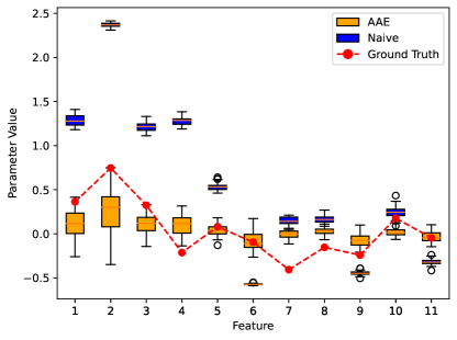
Figure 3: Estimation error of $\hat{\bm{\beta}}^{\sf AAE}$ and $\hat{\bm{\beta}}^{\sf Naive}$ by Feature

Notes:

The figures presents the ground-truth parameters $\bm{\beta}^{*}$ (in the red curve), $\hat{\bm{\beta}}^{\sf AAE}$ (orange box) and $\hat{\bm{\beta}}^{\sf Naive}$ (blue box). The percentiles in the box plots are based on the 50 experimental runs with $m=100$.

5.4 Our Approach v.s. Human-only Data—Financial Value of Our Approach

So far, we have focused on evaluating our method based on estimation error against other ways of utilizing AI data. In practice, the primary goal of using AI as a data augmenter in market research is to reduce the costs of hiring real survey participants. Thus, we evaluated the percentage of data saved using AAE with various GPT models, as summarized in Table 3. Specifically, for a given error reduction achieved by applying AAE to a real dataset of size $n_{1}$, we calculated the amount of real data samples, $n_{2}$, required to achieve the same error reduction without AI augmentation. The percentage of data saved is then estimated as $((n_{2}-n_{1})/n_{2})\times 100\%$.

Our results show that with fine-tuned GPT-4o, data savings range from 24.9% to 79.8%. When the primary set is small ($m=50$), AAE saves between 71.64% and 79.8% of data samples, regardless of the GPT model or prompt design. With a moderate primary set size ($m=100,150$), savings range from 27.7% to 58.0%, again consistent across GPT models and prompts. Compared to the costs of recruiting real survey participants, the costs of generating AI-based data are negligible and will continue to decrease as generative AI technology advances. In practice, conjoint surveys must be regularly re-administered across different product categories and customer segments to account for evolving consumer preferences. This can result in a substantial number of surveys being required over time. Thus, based on our analysis, we conclude that AAE offers significant cost savings in the long run.

Table 3: Percentage of Saving in Data Size (%)

Model	Prompt	$m=50$	$m=100$	$m=150$	$m=200$
GPT-3.5-Turbo-0613	Basic	73.59 (0.69)	46.48 (1.64)	30.97 (1.68)	-0.86 (2.80)*
	CoT	76.05 (1.63)	52.84 (2.61)	37.34 (2.93)	8.37 (4.49)
GPT-3.5-Turbo-0125	Basic	71.64 (0.77)	42.67 (1.63)	27.65 (1.36)	-3.72 (2.75)*
	CoT	77.24 (1.23)	52.44 (1.98)	36.22 (2.19)	10.73 (3.77)
GPT-4	Basic	79.30 (1.20)	53.23 (2.28)	39.83 (2.00)	14.01 (3.17)
	CoT	78.40 (1.68)	53.70 (2.89)	40.76 (2.22)	14.96 (3.78)
GPT-4o	Basic	77.86 (1.56)	51.91 (2.74)	38.10 (2.41)	9.39 (4.35)
	CoT	78.81 (1.45)	52.64 (2.66)	41.02 (2.13)	15.14 (3.82)
	FS	79.39 (1.41)	53.79 (2.56)	42.47 (1.97)	13.00 (3.99)
GPT-4o Fine-tuned	Basic	79.81 (1.63)	58.04 (3.22)	50.20 (2.27)	24.86 (4.16)

Notes:

This table presents the percentage of data saved using AAE with various GPT models, averaged over 50 experimental runs. The standard errors are shown in parentheses. One sample t-tests show that the savings are all significant at the 95% level except for the ones marked with a star.

Furthermore, we calculate the efficient frontier of estimation accuracy and recruitment costs using our methods compared to human-only data. For this analysis, we assume that recruiting each human subject costs $50$ USD, while querying the LLM incurs no cost. Fig. 4 illustrates how AAE extends the efficient frontier for conjoint market research. The yellow line represents the parameter estimation accuracy relative to the total costs of hiring human subjects, indicating the current trade-off between costs and accuracy for traditional conjoint analysis. The blue line shows the accuracy achieved with AAE, where AI-generated labels supplement the corresponding human data, significantly pushing the frontier outward. Additionally, the green line represents the accuracy of naive augmentation with AI data. As observed, naive utilization of AI data does not enhance efficiency. This figure further underscores the practical value of AAE, especially when the sample size is small. We note that, although the sample size may not be small at the population level, market research often focuses on responses from specific demographic groups, where sample sizes are typically smaller. This increases the value of our estimators significantly.

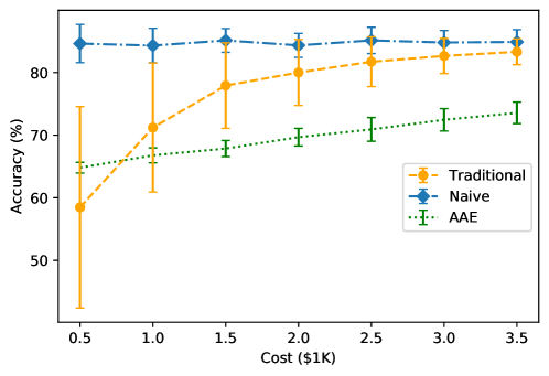
Figure 4: Conjoint estimation accuracy vs. market research costs

Notes:

The plot shows the parameter estimation accuracy (1 - MAPE) relative to the total costs of hiring human subjects with the traditional market research estimator $\hat{\bm{\beta}}^{\sf P}$, the naive estimator $\hat{\bm{\beta}}^{\sf P}$, and the AAE estimator $\hat{\bm{\beta}}^{\sf AAE}$. The average accuracy and error bars are computed over 50 random experimental runs with the same setup in Section 5.1.

6 Empirical Analysis II: Sports Car

In this section, we present an alternative empirical study on a real choice-based conjoint dataset for sports cars (Spencer 2019) as a robustness check for the results in Section 5. The empirical setup is outlined below.

6.1 Empirical Setup

This dataset consists of responses from 200 participants, each expressing preferences for a series of hypothetical sports cars. Every respondent was shown ten sets of three sports cars, described by five attributes with multiple levels, as outlined in Table 4. Participants were asked to choose one of the three cars. We randomly selected 120 respondents from the training set for each experiment, resulting in a dataset of 1,200 samples. The car attributes in these samples were converted to text and used to generate GPT datasets, following the same procedure in Section 5.2. The remainder of the experimental setup is consistent with the approach described in Section 5.1.

The primary difference between the sports car conjoint analysis and the COVID-19 vaccine study is the subjectivity of the choices. While a smaller chance of side effects is a clear preference across the general population in the vaccine context, preferences for a basic versus a racer car model vary based on individual tastes. Since personal demographic information is unavailable in the dataset, we instructed GPT to simulate a random person’s preferences, as we did for the vaccine dataset in Section 5. This experimental setting thus tests the AAE’s performance in handling more subjective choice scenarios.

Table 4: Attributes in the sports car conjoint analysis

Feature	Levels and Description
Segment (Type of car model)	“Basic”, “Fun”, and “Racer” ;
Number of Seats	2, 4, and 5;
Type of transmission	“Manual” and “Automatic”;
Convertible Roofs	“Yes” and “No”
Price	Price in thousands $, with three possible choices (30, 35, 40)

6.2 Conjoint Data Generation using GPT

In this section, we illustrate the conjoint data generation procedure with the sports car conjoint setting, in particular, to show how the previously established framework can be applied in other conjoint settings. The models and prompting follow the same setup as in the previous section.

6.2.1 Basic Prompting

In this part, we present an example of basic prompting following the three-step framework for the sports car data:

Input (I): You should act like a random person purchasing a sports car.
Input (II): There are three options for you:
A: Type of car model: Basic. Number of seats: 2. Type of transmission: Manual. Convertible roofs: Yes. Price: $30k
B: Type of car model: Basic. Number of seats: 4. Type of transmission: Manual. Convertible roofs: Yes. Price: $40k
C: Type of car model: Basic. Number of seats: 4. Type of transmission: Auto. Convertible roofs: Yes. Price: $35k
Input (III): Which option would you choose as a random person? Your response should be a single letter A, B, or C.
Output: B

6.2.2 CoT Prompting

In CoT prompting, we allow GPT to compare the features of cars systematically before reaching a final decision in part (III). An example of the CoT-based conversation is provided below. As illustrated, GPT demonstrates more personal insight when selecting sports cars compared to the vaccine context, with less clearly defined preference rankings involved in comparing each feature.

Input: Compare the number of seats of A, B, and C, which one would you prefer?
Output: Well, I think I’d like option B. You know, the idea of cruising around in a sports car sounds fantastic, but practically speaking, having four seats could be a real benefit. I mean, the chances of me going to a sports event or on a road trip with friends are high. So, the extra seats could come handy then. Plus, it’s not that much costly either. Only $40k, right? I think it’s worth the price.
Input: Compare the type of transmission of A, B, and C, which one would you prefer?
Output: To be honest, I’ve always enjoyed the feeling of control I get with a manual transmission. It makes driving more engaging for me. So, I’m leaning more towards options A or B. But if I consider the number of seats as well…you know, having room for more friends… I’d have to say option B is looking like a better fit for me.
Input: Compare the roof of A, B, and C, which one would you prefer?
Output: All the cars A, B, and C have convertible roofs, which is fantastic. I love the idea of feeling the wind in my hair while cruising down the highway on a sunny day. So, considering the other factors, I’m still leaning toward option B. Hard to beat the full experience it offers - a manual transmission, room for friends, and a convertible roof!
Input: Compare the price of A, B, and C, which one would you prefer?
Output: Option A is the least expensive at $30k, which is quite tempting. But, I think I’d still stick with option B. It might be $10k more, but it also offers two extra seats and the joy of manual driving, which fit my preferences better. I see it as an investment in fun experiences with friends and personal enjoyment when driving. It’s looking like a worthwhile expenditure.
Input: Based on all the previous reasonings, which option would you choose?
Output: Based on all the comparisons around the number of seats, transmission type, roof, and price, I would choose Option B. It might be a bit more expensive, but it fits my needs in terms of the extra seating, manual transmission, and the awesome convertible roof.
Input: Return the choice in the previous answer as a single letter A, B, or C.
Output: B

6.3 Empirical Results

Table 5 summarizes the change in MAPE of $\hat{\bm{\beta}}^{\sf A}$, $\hat{\bm{\beta}}^{\sf Naive}$, and $\hat{\bm{\beta}}^{\sf AAE}$ using $\hat{\bm{\beta}}^{\sf P}$ as the benchmark. Similar to the findings in Section 5, AAE significantly reduces MAPE across all scenarios, achieving in general the best performance using GPT-4 with CoT and GPT-4o with few-shot prompting, while the naive method tends to elicit errors. Interestingly, AAE’s performance shows less correlation with higher versions of GPT and CoT in comparison to the vaccine setting, which is expected given that sports car preferences are highly subjective. Despite being an older version, GPT-3.5-Turbo-0613 performs well with AAE in this context. One can notice that GPT-3.5-Turbo-0613 incurs a small estimation error with naive augmentation, suggesting it may happen to have a close alignment with real human data, which in turn enhances AAE’s effectiveness. On the other hand, Naive does not exhibit a consistent correlation with higher versions of GPT and performs significantly worse after implementing CoT. This type of result is common in choice data heavily influenced by personal tastes rather than rational decision-making, as is the case with sports car selection. Moreover, fine-tuning GPT-4o does not improve the performance of naive augmentation. This underscores that fine-tuning is not a universal solution to all problems.

Table 5: Change in MAPE per feature in empirical setting II(%)

		$m=50$			$m=100$			$m=150$			$m=200$
Model	Prompt	A	Naive	AAE	A	Naive	AAE	A	Naive	AAE	A	Naive	AAE
GPT-3.5- Turbo-0613	Basic	-17.27	-34.20	-37.81	15.09	-1.15	-11.02	28.53	8.57	-6.83	30.71	8.26	-7.09
	CoT	148.81	119.98	-34.33	181.18	130.32	-9.50	194.62	126.11	-4.80	196.80	119.07	-5.39
GPT-3.5- Turbo-0125	Basic	29.70	5.58	-30.22	62.06	32.47	-9.80	75.50	37.96	-5.30	77.68	34.69	-6.59
	CoT	129.80	112.47	-35.35	162.17	124.39	-11.07	175.60	123.92	-5.17	177.78	113.93	-6.64
GPT-4	Basic	-12.43	-16.70	-30.63	19.94	10.17	-8.62	33.37	21.31	-4.60	35.55	19.68	-4.72
	CoT	173.34	132.71	-38.32	205.71	137.60	-11.36	219.15	136.34	-7.69	221.32	121.56	-6.62
GPT-4o	Basic	421.27	292.59	-25.68	453.64	263.41	-8.92	467.07	234.85	-4.56	469.25	207.47	-7.03
	CoT	304.98	229.80	-28.65	337.34	219.76	-7.86	350.78	199.59	-5.92	352.96	178.51	-6.26
	FS	201.95	133.85	-36.74	234.32	132.10	-12.85	247.76	123.92	-9.02	249.93	110.30	-6.99
GPT-4o Fine-tuned	Basic	153.33	89.90	-31.61	185.69	98.61	-8.45	199.13	96.48	-2.84	201.31	84.70	-4.38

Table 6 shows the percentage of data that can be saved using AAE. Our results show data savings ranging from 12.7% to 61.9% across different models, prompts, and primary data sizes. When the primary set is small ($m=50$), AAE saves between 44.1% and 61.9% of data samples, regardless of the GPT model or prompt design. With a moderate primary set size ($m=100,150$), savings range from 21.8% to 41.6%, again consistent across GPT models and prompts. These results further support the practical value of AAE in broad conjoint settings.

Table 6: Percentage of saving in data size in empirical setting II(%)

Model	Prompt	$m=50$	$m=100$	$m=150$	$m=200$
GPT-3.5-Turbo-0613	Basic	60.08	38.94	35.00	18.60
	CoT	55.27	36.57	28.71	15.00
GPT-3.5-Turbo-0125	Basic	49.01	37.05	30.92	17.58
	CoT	56.78	39.00	30.35	17.67
GPT-4	Basic	49.41	35.11	27.76	13.49
	CoT	61.88	39.45	36.45	17.64
GPT-4o	Basic	44.09	35.61	27.58	18.49
	CoT	47.40	33.79	33.38	16.89
	FS	58.68	41.57	38.58	18.40
GPT-4o Fine-tuned	Basic	50.67	34.81	21.82	12.71

7 Conclusion

This paper presents a new approach for incorporating LLM-generated data into conjoint analysis, addressing the growing need for scalable and cost-effective methods in market research. While LLMs can mimic human-like responses, our study underscores the persistent errors and limitations inherent in directly using these AI-generated responses. Through our proposed data augmentation framework, which combines LLM-generated labels with real data, we demonstrate that it is possible to extract valuable insights from AI-generated data while mitigating errors that can distort market research outcomes. Our theoretical framework, inspired by knowledge distillation and transfer learning, establishes a method to transfer the valuable but imperfect knowledge embedded in LLMs into a simpler, aligned model. This approach is validated empirically, where we show that our estimator not only reduces errors but also achieves significant data savings. Importantly, our findings highlight that while state-of-the-art LLMs, such as GPT-4, can improve the quality of AI-generated labels, their usefulness ultimately depends on how well they are integrated with real data.

Looking ahead, our method opens the door for more effective use of LLMs in market research and beyond. As LLM technology advances, this framework can serve as a foundation for further innovations in data augmentation, helping researchers and practitioners balance the trade-offs between AI-generated and human-generated data. Future work may explore how this approach can be extended to other domains where real data is scarce, unlocking new applications for AI in understanding human preferences and behaviors. Future work could explore additional ways to enhance the usability of LLMs in combination with our methods. For instance, a promising research direction is examining the impact of incorporating different personas into LLM queries to generate data that more closely resembles a specific set of users. Finally, while our paper focuses on conjoint analysis, the underlying theory applies more broadly to other knowledge distillation tasks involving LLMs, such as transferring knowledge from a teacher model to a student model. This opens up promising opportunities to generalize our ideas to other contexts and explore their statistical properties.

Online Appendix

Harnessing Large Language Models for Market Research: A Data-augmentation Approach

8 Supporting Arguments to Section 4

Lemma 8.1 (Derivative Computation)

Suppose that $\bm{\alpha}\in\mathbb{R}^{k+1}_{+}$ satisfies $\sum_{j\in\mathcal{K}^{+}}\alpha_{j}=1$. Then

$$\nabla_{\bm{\beta}}\left(\sum_{j\in\mathcal{K}^{+}}\alpha_{j}\sigma_{j}(\mathbf{x};\bm{\beta})\right)~{}=~{}\sum_{j\in\mathcal{K}}(\alpha_{j}-\sigma_{j}(\mathbf{x};\bm{\beta}))\mathbf{x}_{j}~{}~{}\text{ and }~{}~{}\nabla_{\bm{\beta}}^{2}\left(\sum_{j\in\mathcal{K}^{+}}\alpha_{j}\sigma_{j}(\mathbf{x};\bm{\beta})\right)~{}=~{}-\mathbf{A}(\mathbf{x};\bm{\beta}).$$

Proof. The proof of this lemma follows from straightforward computation and we skip the details. $\blacksquare$

Lemma 8.2 (Bounds on the Quadratic Form)

Let us fix any $\mathbf{x}\in\mathcal{X}$, $\bm{\beta}\in\mathbb{R}^{k}$, and $\mathbf{u}\in\mathbb{R}^{k}$.

$$\sigma_{0}(\mathbf{x};\bm{\beta})\min_{j\in\mathcal{K}}\sigma_{j}(\mathbf{x};\bm{\beta})\sum_{j\in\mathcal{K}}(\mathbf{x}_{(j)}\mathbf{u})^{2}~{}\leq~{}\mathbf{u}^{\top}\mathbf{A}(\mathbf{x};\bm{\beta})\mathbf{u}~{}\leq~{}\sigma_{0}(\mathbf{x};\bm{\beta})\max_{j\in\mathcal{K}}\sigma_{j}(\mathbf{x};\bm{\beta})\sum_{j\in\mathcal{K}}(\mathbf{x}_{(j)}\mathbf{u})^{2}.$$

Proof. Define matrix $\bm{\Sigma}(\mathbf{x};\bm{\beta})\in\mathbb{R}^{d\times d}$ such that $\bm{\Sigma}_{jj^{\prime}}(\mathbf{x};\bm{\beta})=\mathbbm{1}_{\{j=j^{\prime}\}}\sigma_{j}(\mathbf{x};\bm{\beta}^{*})-\sigma_{j}(\mathbf{x};\bm{\beta})\sigma_{j^{\prime}}(\mathbf{x},\bm{\beta})$ for each $1\leq j,j^{\prime}\leq d$. Then, $\mathbf{u}^{\top}\mathbf{A}(\mathbf{x};\bm{\beta})\mathbf{u}=\sum_{j\in\mathcal{K}}\sum_{j^{\prime}\in\mathcal{K}}\bm{\Sigma}_{jj^{\prime}}(\mathbf{x};\bm{\beta})(\mathbf{x}_{(j)}^{\top}\mathbf{u})(\mathbf{x}_{(j)}^{\top}\mathbf{u})$. Therefore, it sufficies to show that

$$\sigma_{0}(\mathbf{x};\bm{\beta})\min_{j\in\mathcal{K}}\sigma_{j}(\mathbf{x};\bm{\beta})\mathbf{I}~{}\preceq~{}\bm{\Sigma}(\mathbf{x};\bm{\beta})~{}\preceq~{}\sigma_{0}(\mathbf{x};\bm{\beta})\max_{j\in\mathcal{K}}\sigma_{j}(\mathbf{x};\bm{\beta})\mathbf{I}.$$

Indeed, by the Gershgorin circle theorem, it holds that any eigenvalue $\lambda$ of $\bm{\Sigma}$ satisfies

$$\sigma_{0}(\mathbf{x};\bm{\beta})\min_{j\in\mathcal{K}}\sigma_{j}(\mathbf{x};\bm{\beta})~{}=~{}\min_{j\in\mathcal{K}}\left\{\sigma_{j}(\mathbf{x};\bm{\beta})-\sum_{j^{\prime}\in\mathcal{K}}\sigma_{j}(\mathbf{x};\bm{\beta})\sigma_{j^{\prime}}(\mathbf{x};\bm{\beta})\right\}~{}\leq~{}\lambda$$

$$~{}~{}~{}~{}~{}~{}~{}~{}~{}~{}~{}~{}~{}~{}~{}~{}~{}~{}~{}~{}~{}~{}~{}~{}~{}~{}~{}~{}~{}~{}~{}~{}~{}~{}~{}~{}~{}~{}~{}~{}~{}~{}~{}~{}~{}~{}~{}~{}~{}~{}~{}~{}~{}~{}~{}~{}~{}~{}~{}~{}\leq~{}\max_{j\in\mathcal{K}}\left\{\sigma_{j}(\mathbf{x};\bm{\beta})-\sum_{j^{\prime}\in\mathcal{K}}\sigma_{j}\sigma_{j^{\prime}}(\mathbf{x};\bm{\beta})\right\}=\sigma_{0}(\mathbf{x};\bm{\beta})\max_{j\in\mathcal{K}}\sigma_{j}(\mathbf{x};\bm{\beta}).$$

Therefore, we conclude the poof. $\blacksquare$

Proof of Lemma 4.5. We first show that there exists at least an optimizer. Assume that there exists $\{\bm{\beta}^{(\ell)}\}_{\ell=1}^{\infty}$ such that

$$\lim_{\ell\rightarrow\infty}\mathbb{E}_{\mathbf{x}}\Big{[}{\sf KL}\big{(}\mathbb{P}(y\,|\,\mathbf{x})\,\big{|}\,\sigma_{y}(\mathbf{x},\bm{\beta}^{(\ell)})\big{)}\Big{]}~{}=~{}\inf_{\bm{\beta}\in\mathbb{R}^{kd}}\mathbb{E}_{\mathbf{x}}\Big{[}{\sf KL}\big{(}\mathbb{P}(y\,|\,\mathbf{x})\,\big{|}\,\sigma_{y}(\mathbf{x},\bm{\beta})\big{)}\Big{]},$$

or equivalently

$$\lim_{\ell\rightarrow\infty}\mathbb{E}_{\mathbf{x}}\left[\sum_{j\in\mathcal{K}^{+}}\mathbb{P}\big{(}y=j|\mathbf{x}\big{)}\log\sigma_{j}(\mathbf{x},\bm{\beta}^{(\ell)})\right]~{}=~{}\sup_{\bm{\beta}\in\mathbb{R}^{k}}Q(\bm{\beta})~{}=~{}\sup_{\bm{\beta}\in\mathbb{R}^{k}}\mathbb{E}_{\mathbf{x}}\left[\sum_{j\in\mathcal{K}^{+}}\mathbb{P}\big{(}y=j|\mathbf{x}\big{)}\log\sigma_{j}(\mathbf{x},\bm{\beta}^{(\ell)})\right],$$ (8)

If there is a subsequence of $\{\bm{\beta}^{(\ell)}\}_{\ell=1}^{\infty}$ that is bounded, by the continuity of $\mathbb{E}_{\mathbf{x}}\Big{[}{\sf KL}\big{(}\mathbb{P}(y\,|\,\mathbf{x})\,\big{|}\,\sigma_{y}(\mathbf{x},\bm{\beta})\big{)}\Big{]}$, there must exist a limit of a subsequence of $\{\bm{\beta}^{(\ell)}\}_{\ell=1}^{\infty}$ such that the infimum is achieved. This proves the existence.

Otherwise, let us assume that $\{\bm{\beta}^{(\ell)}\}_{\ell=1}^{\infty}$ is unbounded, so $\lim_{\ell\rightarrow\infty}\lVert\bm{\beta}^{(\ell)}\rVert_{2}=\infty$. We will show that this is impossible, by way of contradiction. Since $\{\bm{\beta}^{(\ell)}/\lVert\bm{\beta}^{(\ell)}\rVert_{2}\}_{\ell=1}^{\infty}$ is a bounded sequence, by taking a subsequence if necessary, we can assume without loss of generality that $\lim_{\ell\rightarrow\infty}\bm{\beta}^{(\ell)}/\lVert\bm{\beta}^{(\ell)}\rVert_{2}=\tilde{\bm{\beta}}$ with $\lVert\tilde{\bm{\beta}}\rVert_{2}=1$. Thus,

$$\lim_{\ell\rightarrow\infty}\mathbb{E}_{\mathbf{x}}\left[\max_{j\in\mathcal{K}}\big{|}(\bm{\beta}^{(\ell)})^{\top}\mathbf{x}_{(j)}\big{|}\right] ~{}\geq~{}\frac{1}{k}\lim_{\ell\rightarrow\infty}\mathbb{E}_{\mathbf{x}}\left[\sum_{j\in\mathcal{K}}\big{|}(\bm{\beta}^{(\ell)})^{\top}\mathbf{x}_{(j)}\big{|}\right]~{}=~{}\frac{1}{k}\lim_{\ell\rightarrow\infty}\lVert\bm{\beta}^{(\ell)}\rVert_{2}\cdot\mathbb{E}_{\mathbf{x}}\left[\sum_{j\in\mathcal{K}}\left|\frac{(\bm{\beta}^{(\ell)})^{\top}}{\lVert\bm{\beta}^{(\ell)}\rVert_{2}}\mathbf{x}_{(j)}\right|\right]$$

$$~{}\stackrel{{\scriptstyle\text{(a)}}}{{=}}~{}\frac{1}{k}\mathbb{E}_{\mathbf{x}}\left[\sum_{j\in\mathcal{K}}\left|\tilde{\bm{\beta}}^{\top}\mathbf{x}_{(j)}\right|\right]\cdot\lim_{\ell\rightarrow\infty}\lVert\bm{\beta}^{(\ell)}\rVert_{2}~{}=~{}\frac{1}{k}\mathbb{E}_{\mathbf{x}}\left[\sum_{j\in\mathcal{K}}\left|\tilde{\bm{\beta}}^{\top}\mathbf{x}_{(j)}\right|\right]\cdot+\infty~{}\stackrel{{\scriptstyle\text{(b)}}}{{=}}~{}\infty,$$ (9)

where (a) follows from the bounded convergence theorem because by assumption $\mathbf{x}$ is bounded. To see (b), suppose that $\mathbb{E}_{\mathbf{x}}\left[\sum_{j\in\mathcal{K}}\left|\tilde{\bm{\beta}}^{\top}\mathbf{x}_{(j)}\right|\right]=0$. Thus, $\tilde{\bm{\beta}}^{\top}\mathbf{x}_{(j)}=0$ for all $j\in\mathcal{K}$ almost everywhere. Thus, if we let $\mathbf{u}$ denote a vector of ones of dimension $k$, we have $(\bm{\beta}\otimes\mathbf{u})\mathbb{E}_{\mathbf{x}}[\mathbf{x}\mathbf{x}^{\top}](\bm{\beta}\otimes\mathbf{u})^{\top}=0$, which contradicts the assumption that $\mathbb{E}_{\mathbf{x}}[\mathbf{x}\mathbf{x}^{\top}]$ is positive definite.

We note that by the Taylor expansion, for any $u\in\mathbb{R}$ and $v\in[0,k]$,

$$\log\frac{e^{u}}{v+e^{u}}~{}=~{}u-\log\left(v+e^{u}\right)~{}=~{}u-\left[\log(v+1)+\frac{u}{v+1}+\frac{ve^{{w}}u^{2}}{2(e^{w}+v)^{2}}\right]~{}\stackrel{{\scriptstyle\text{(c)}}}{{\leq}}~{}\frac{ku}{k+1},$$ (10)

where $w\in[u,v]$ and (c) follows because $\frac{ve^{{w}}u^{2}}{2(e^{w}+v)^{2}}\geq 0$, $\log(v+1)\geq 0$ and $v\leq k$.

Next, fix $\ell=1,\dots,\infty$ and $\mathbf{x}\in\mathcal{X}$. We assume that $\tilde{j}\in\mathcal{K}$ is such that $\tilde{j}=\argmax_{j^{\prime}\in\mathcal{K}}\big{|}(\bm{\beta}^{(\ell)})^{\top}\mathbf{x}_{(j^{\prime})}\big{|}$. If $(\bm{\beta}^{(\ell)})^{\top}\mathbf{x}_{(\tilde{j})}>0$, it follows that

$$\sum_{j\in\mathcal{K}^{+}}\mathbb{P}\big{(}y=j|\mathbf{x}\big{)}\log\sigma_{j}(\mathbf{x},\bm{\beta}^{(\ell)})~{}\leq~{}\mathbb{P}\big{(}y=0\,|\,\mathbf{x}\big{)}\log\sigma_{0}(\mathbf{x},\bm{\beta}^{(\ell)})$$

$$~{}~{}~{}~{}~{}~{}~{}~{}~{}~{}~{}~{}~{}~{}~{}~{}~{}~{}=~{}\mathbb{P}\big{(}y=0\,|\,\mathbf{x}\big{)}\log\left(\frac{e^{-(\bm{\beta}^{(\ell)})^{\top}\mathbf{x}_{(\tilde{j})}}}{e^{-(\bm{\beta}^{(\ell)})^{\top}\mathbf{x}_{(\tilde{j})}}+\sum_{j\in\mathcal{K}}e^{-(\bm{\beta}^{(\ell)})^{\top}\mathbf{x}_{(\tilde{j})}+(\bm{\beta}^{(\ell)})^{\top}\mathbf{x}_{(j)}}}\right)~{}\stackrel{{\scriptstyle\text{(d)}}}{{\leq}}~{}\frac{-k\big{|}(\bm{\beta}^{(\ell)})^{\top}\mathbf{x}_{(\tilde{j})}\big{|}}{k+1},$$

where (d) follows from (10) because $-(\bm{\beta}^{(\ell)})^{\top}\mathbf{x}_{(\tilde{j})}+(\bm{\beta}^{(\ell)})^{\top}\mathbf{x}_{(j)}\leq 0$. Suppose $(\bm{\beta}^{(\ell)})^{\top}\mathbf{x}_{(j)}\leq 0$ for all $j\in\mathcal{K}$. Then, we have

$$\sum_{j\in\mathcal{K}^{+}}\mathbb{P}\big{(}y=j\,|\,\mathbf{x}\big{)}\log\sigma_{j}(\mathbf{x},\bm{\beta}^{(\ell)})~{}\leq~{}\mathbb{P}\big{(}y=\tilde{j}\,|\,\mathbf{x}\big{)}\log\sigma(\mathbf{x},\bm{\beta}^{(\ell)})$$

$$~{}~{}~{}~{}~{}~{}~{}~{}~{}~{}~{}~{}~{}~{}~{}~{}~{}~{}~{}~{}~{}~{}~{}~{}~{}~{}~{}~{}~{}~{}~{}~{}~{}~{}~{}~{}~{}~{}~{}~{}~{}~{}=~{}\mathbb{P}\big{(}y=\tilde{j}\,|\,\mathbf{x}\big{)}\log\left(\frac{e^{(\bm{\beta}^{(\ell)})^{\top}\mathbf{x}_{(\tilde{j})}}}{1+\sum_{j\in\mathcal{K}}e^{(\bm{\beta}^{(\ell)})^{\top}\mathbf{x}_{({j})}}}\right)~{}\stackrel{{\scriptstyle\text{(e)}}}{{\leq}}~{}\frac{-k\big{|}(\bm{\beta}^{(\ell)})^{\top}\mathbf{x}_{(\tilde{j})}\big{|}}{k+1},$$

where (e) follows from (10). Suppose $(\bm{\beta}^{(\ell)})^{\top}\mathbf{x}_{(\tilde{j})}\leq 0$ but $(\bm{\beta}^{(\ell)})^{\top}\mathbf{x}_{({j}^{\prime\prime})}>0$ for some $j^{\prime\prime}\in\mathcal{K}$ and $(\bm{\beta}^{(\ell)})^{\top}\mathbf{x}_{({j}^{\prime\prime})}\geq(\bm{\beta}^{(\ell)})^{\top}\mathbf{x}_{({j})}$ for all $j\in\mathcal{K}$. In this case,

$$~{}~{}~{}\sum_{j\in\mathcal{K}^{+}}\mathbb{P}\big{(}y=j\,|\,\mathbf{x}\big{)}\log\sigma_{j}(\mathbf{x},\bm{\beta}^{(\ell)})~{}\leq~{}\mathbb{P}\big{(}y=\tilde{j}\,|\,\mathbf{x}\big{)}\log\sigma_{j^{\prime}}(\mathbf{x},\bm{\beta}^{(\ell)})$$

$$~{}=~{}\mathbb{P}\big{(}y=\tilde{j}\,|\,\mathbf{x}\big{)}\log\left(\frac{e^{(\bm{\beta}^{(\ell)})^{\top}\mathbf{x}_{(\tilde{j})}-(\bm{\beta}^{(\ell)})^{\top}\mathbf{x}_{({j}^{\prime\prime})}}}{e^{-(\bm{\beta}^{(\ell)})^{\top}\mathbf{x}_{({j}^{\prime\prime})})^{\top}\mathbf{x}}+\sum_{j\in\mathcal{K}}e^{-(\bm{\beta}^{(\ell)})^{\top}\mathbf{x}_{({j}^{\prime\prime})}+(\bm{\beta}^{(\ell)})^{\top}\mathbf{x}_{({j})}}}\right)~{}\stackrel{{\scriptstyle\text{(f)}}}{{\leq}}~{}\frac{k\big{(}(\bm{\beta}^{(\ell)})^{\top}\mathbf{x}_{(\tilde{j})}-(\bm{\beta}^{(\ell)})^{\top}\mathbf{x}_{({j}^{\prime\prime})}x\big{)}}{k+1}$$

$$~{}\leq~{}\frac{-k\big{|}(\bm{\beta}^{(\ell)}_{\tilde{j}})^{\top}\mathbf{x}\big{|}}{k+1},$$

where (f) follows from (10) again. To summarize, taking the expectation, using (8), we have

$$\lim_{\ell\rightarrow\infty}\mathbb{E}_{\mathbf{x}}\left[\sum_{j\in\mathcal{K}^{+}}\mathbb{P}\big{(}y=j|\mathbf{x}\big{)}\log\sigma_{j}(\mathbf{x},\bm{\beta}^{(\ell)})\right]~{}\leq~{}-\lim_{\ell\rightarrow\infty}\mathbb{E}_{\mathbf{x}}\left[\frac{k\max_{j\in\mathcal{K}}\big{|}(\bm{\beta}^{(\ell)})^{\top}\mathbf{x}_{({j})}\big{|}}{k+1}\right]=-\infty.$$

This contradicts (8). Therefore, $\{\bm{\beta}^{(\ell)}\}_{\ell=1}^{\infty}$ cannot be unbounded. This finishes the proof of existence.

Next, using Lemma 8.1, we notice the Hession of $\mathbb{E}_{\mathbf{x}}\left[\sum_{j\in\mathcal{K}^{+}}\mathbb{P}\big{(}y=j|\mathbf{x}\big{)}\log\sigma_{j}(\mathbf{x};\bm{\beta})\right]$ is $-\widetilde{\bm{\Omega}}(\bm{\beta})$, where $\widetilde{\bm{\Omega}}(\bm{\beta})~{}:=~{}\mathbb{E}_{\mathbf{x}}\left[\mathbf{A}(\mathbf{x};\bm{\beta})\right]\in\mathbb{R}^{k\times k}$, which is analogous to $\bm{\Omega}$ defined in (4). Thus, take any $\mathbf{q}\in\mathbb{R}^{k}$ such that $\lVert\mathbf{q}\rVert_{2}=1$. Thus, for any $\bm{\beta}\in\mathbb{R}^{k}$

$$\mathbf{q}^{\top}\left(-\nabla^{2}_{\bm{\beta}}\mathbb{E}_{\mathbf{x}}\left[\sum_{j\in\mathcal{K}^{+}}\mathbb{P}\big{(}y=j|\mathbf{x}\big{)}\log\sigma_{j}(\mathbf{x};\bm{\beta})\right]\right)\mathbf{q}\,=\,\mathbb{E}_{\mathbf{x}}\left[\mathbf{q}^{\top}\mathbf{A}(\mathbf{x};\bm{\beta})\mathbf{q}^{\top}\right]\stackrel{{\scriptstyle\text{(g)}}}{{\geq}}\mathbb{E}_{\mathbf{x}}\left[\sigma_{0}(\mathbf{x};\bm{\beta})\min_{j\in\mathcal{K}}\sigma_{j}(\mathbf{x};\bm{\beta})\sum_{j\in\mathcal{K}}(\mathbf{x}^{\top}\mathbf{q})^{2}\right]$$

$$~{}~{}~{}~{}~{}~{}~{}~{}~{}~{}~{}~{}~{}~{}~{}~{}~{}~{}~{}~{}~{}~{}~{}~{}~{}~{}~{}~{}~{}~{}~{}~{}~{}~{}~{}~{}~{}~{}~{}~{}~{}~{}~{}~{}~{}~{}~{}~{}\stackrel{{\scriptstyle\text{(h)}}}{{\succsim}}\sum_{j\in\mathcal{K}}\mathbb{E}_{\mathbf{x}}\left[\sum_{j\in\mathcal{K}}(\mathbf{x}^{\top}\mathbf{q})^{2}\right]\stackrel{{\scriptstyle\text{(i)}}}{{\geq}}\,\lambda_{\min}\left(\mathbb{E}_{\mathbf{x}}[\mathbf{x}\mathbf{x}^{\top}]\right)k\lVert\mathbf{q}\rVert^{2}=k\lambda_{\min}\left(\mathbb{E}_{\mathbf{x}}[\mathbf{x}\mathbf{x}^{\top}]\right),$$

where (g) follows from Lemma 8.2, (h) follows because $\mathbf{x}$ is bounded, and in (i), $\lambda_{\min}\left(\mathbb{E}_{\mathbf{x}}[\mathbf{x}\mathbf{x}^{\top}]\right)$ is the smallest eigenvalue of $\mathbb{E}_{\mathbf{x}}[\mathbf{x}\mathbf{x}^{\top}]$. Therefore, the function $\mathbb{E}_{\mathbf{x}}\left[\sum_{j\in\mathcal{K}^{+}}\mathbb{P}\big{(}y=j|\mathbf{x}\big{)}\log\sigma_{j}(\mathbf{x};\bm{\beta})\right]$ is strictly concave and has a unique maximum. This concludes the proof. $\blacksquare$

Proof of Lemma 4.6. Our proof starts with the decomposition:

$$\sup_{\bm{\beta}\in\mathcal{B}(\bm{\beta}^{*},\epsilon_{1})}\left|\widehat{Q}(\hat{\bm{\theta}};\bm{\beta})-{Q}(\bm{\beta})\right|~{}\leq~{}\sup_{\bm{\beta}\in\mathcal{B}(\bm{\beta}^{*},\epsilon_{1})}\left|\widehat{Q}(\hat{\bm{\theta}};\bm{\beta})-\widehat{Q}({\theta}^{*};\bm{\beta})\right|+\sup_{\bm{\beta}\in\mathcal{B}(\bm{\beta}^{*},\epsilon_{1})}\left|\widehat{Q}({\theta}^{*};\bm{\beta})-{Q}(\bm{\beta})\right|.$$ (11)

Then,

$$\sup_{\bm{\beta}\in\mathcal{B}(\bm{\beta}^{*},\epsilon_{1})}\left|\widehat{Q}(\hat{\bm{\theta}};\bm{\beta})-\widehat{Q}({\theta}^{*};\bm{\beta})\right|$$

$$~{}~{}~{}~{}~{}~{}~{}~{}~{}~{}~{}~{}~{}~{}~{}~{}~{}~{}~{}~{}~{}~{}~{}~{}~{}~{}~{}~{}=~{}\sup_{\bm{\beta}\in\mathcal{B}(\bm{\beta}^{*},\epsilon_{1})}\left|\frac{1}{n}\sum_{i=1}^{n}\sum_{j\in\mathcal{K}^{+}}g_{j}(\mathbf{x}_{i},z_{i};\hat{\bm{\theta}})\log\sigma_{j}(\mathbf{x};\bm{\beta})-\frac{1}{n}\sum_{i=1}^{n}\sum_{j\in\mathcal{K}^{+}}g_{j}(\mathbf{x}_{i},z_{i};{\bm{\theta}}^{*})\log\sigma_{j}(\mathbf{x};\bm{\beta})\right|$$

$$~{}~{}~{}~{}~{}~{}~{}~{}~{}~{}~{}~{}~{}~{}~{}~{}~{}~{}~{}~{}~{}~{}~{}~{}~{}~{}~{}~{}\leq~{}\left(\sup_{\mathbf{x}\in\mathcal{X},\,\bm{\beta}\in\mathcal{B}(\bm{\beta}^{*},\epsilon_{1}),\,j\in\mathcal{K}^{+}}\left|\log\sigma_{j}(\mathbf{x};\bm{\beta})\right|\right)\times\sum_{j\in\mathcal{K}^{+}}\frac{1}{n}\sum_{i=1}^{n}\left|g_{j}(\mathbf{x}_{i},z_{i};\hat{\bm{\theta}})-g_{j}(\mathbf{x}_{i},z_{i};{\bm{\theta}}^{*})\right|$$

$$~{}~{}~{}~{}~{}~{}~{}~{}~{}~{}~{}~{}~{}~{}~{}~{}~{}~{}~{}~{}~{}~{}~{}~{}~{}~{}~{}~{}\stackrel{{\scriptstyle(a)}}{{=}}~{}C_{1}\sum_{j\in\mathcal{K}^{+}}\frac{1}{n}\sum_{i=1}^{n}\left|g_{j}(\mathbf{x}_{i},z_{i};\hat{\bm{\theta}})-g_{j}(\mathbf{x}_{i},z_{i};{\bm{\theta}}^{*})\right|,$$

where in $(a)$ we simply define constant $C_{1}=\sup_{\mathbf{x}\in\mathcal{X},\,\bm{\beta}\in\mathcal{B}(\bm{\beta}^{*},\epsilon_{1}),\,j\in\mathcal{K}^{+}}\left|\log\sigma_{j}(\mathbf{x};\bm{\beta})\right|<\infty$ because $\mathcal{X}$ is bounded. Next, fix any $\epsilon_{3}>0$ and any $j\in\mathcal{K}^{+}$.

Consider any sequence $\{\tilde{\bm{\theta}}_{p}\}_{p=1}^{\infty}$ with $\tilde{\bm{\theta}}_{p}\rightarrow\bm{\theta}^{*}$. By the continuity of $g_{j}(\mathbf{x},z;{\bm{\theta}})$ in ${\bm{\theta}}$, and the bounded convergence theorem, it must be that

$$\mathbb{E}_{\mathbf{x},z}\big{[}\left|g_{j}(\mathbf{x},z;{\bm{\theta}}_{p})-g_{j}(\mathbf{x},z;{\bm{\theta}}^{*})\right|\big{]}~{}\rightarrow~{}\mathbb{E}_{\mathbf{x},z}\big{[}\left|g_{j}(\mathbf{x},z;{\bm{\theta}}^{*})-g_{j}(\mathbf{x},z;{\bm{\theta}}^{*})\right|\big{]}=0.$$

In other words, the function $\mathbb{E}_{\mathbf{x},z}\big{[}\left|g_{j}(\mathbf{x},z;{\bm{\theta}})-g_{j}(\mathbf{x},z;{\bm{\theta}}^{*})\right|\big{]}$ is continuous in $\bm{\theta}$. By the continuous mapping theorem, since $\hat{\bm{\theta}}\overset{\text{{P}}}{\rightarrow}\bm{\theta}^{*}$, and the Markov’s inequality, we have

$$\mathbb{P}\left(\frac{1}{n}\sum_{i=1}^{n}\left|g_{j}(\mathbf{x}_{i},z_{i};\hat{\bm{\theta}})-g_{j}(\mathbf{x}_{i},z_{i};{\bm{\theta}}^{*})\right|\geq\epsilon_{3}\,\bigg{|}\,\hat{\bm{\theta}}\right)~{}\leq~{}\frac{1}{\epsilon_{3}}\mathbb{E}_{\mathbf{x},z}\left[\left|g_{j}(\mathbf{x},z;\hat{\bm{\theta}})-g_{j}(\mathbf{x},z;{\bm{\theta}}^{*})\right|\,\bigg{|}\,\hat{\bm{\theta}}\right]\overset{\text{{P}}}{\rightarrow}0.$$

Then we notice that $\mathbb{P}\left(\frac{1}{n}\sum_{i=1}^{n}\left|g_{j}(\mathbf{x}_{i},z_{i};\hat{\bm{\theta}})-g_{j}(\mathbf{x}_{i},z_{i};{\bm{\theta}}^{*})\right|\geq\epsilon_{3}\,\bigg{|}\,\hat{\bm{\theta}}\right)\leq 1$ so it is uniformly integrable. Therefore,

$$\mathbb{P}\left(\frac{1}{n}\sum_{i=1}^{n}\left|g_{j}(\mathbf{x}_{i},z_{i};\hat{\bm{\theta}})-g_{j}(\mathbf{x}_{i},z_{i};{\bm{\theta}}^{*})\right|\geq\epsilon_{3}\right)~{}=~{}\mathbb{E}\left[\mathbb{P}\left(\frac{1}{n}\sum_{i=1}^{n}\left|g_{j}(\mathbf{x}_{i},z_{i};\hat{\bm{\theta}})-g_{j}(\mathbf{x}_{i},z_{i};{\bm{\theta}}^{*})\right|\geq\epsilon_{3}\,\bigg{|}\,\hat{\bm{\theta}}\right)\right]$$

and the right-hand side converges to zero. Therefore,

$$\sup_{\bm{\beta}\in\mathcal{B}(\bm{\beta}^{*},\epsilon_{1})}\left|\widehat{Q}(\hat{\bm{\theta}};\bm{\beta})-\widehat{Q}({\theta}^{*};\bm{\beta})\right|~{}\overset{\text{{P}}}{\rightarrow}~{}0.$$ (12)

We note that $\widehat{Q}({\theta}^{*};\bm{\beta})$ converges to ${Q}(\bm{\beta})$ for each $\bm{\beta}\in\mathbb{R}^{d}$ by the law of large numbers. Then since $\widehat{Q}({\theta}^{*};\bm{\beta})$ is concave in $\bm{\beta}$, by Theorem 2.7 in Newey and McFadden (1994), it holds that on the compact set $\mathcal{B}(\bm{\beta}^{*},\epsilon_{1})$,

$$\sup_{\bm{\beta}\in\mathcal{B}(\bm{\beta}^{*},\epsilon_{1})}\left|\widehat{Q}({\theta}^{*};\bm{\beta})-{Q}(\bm{\beta})\right|\overset{\text{{P}}}{\rightarrow}0.$$ (13)

Combining (11), (12) and (13), the conclusion follows. $\blacksquare$

Proof of Lemma 4.7. For any $\mathbf{x}\in\mathcal{X}$ and $\bm{\beta}\in\mathbb{R}^{kd}$, we note that

$$\sum_{j\in\mathcal{K}^{+}}g_{j}(\mathbf{x},z;{\bm{\theta}})\nabla^{2}_{\bm{\beta}}\log\sigma_{j}(\mathbf{x};{\bm{\beta}})~{}=~{}\nabla^{2}_{\bm{\beta}}\left(\sum_{j\in\mathcal{K}^{+}}g_{j}(\mathbf{x},z;{\bm{\theta}})\right)\log\sigma_{j}(\mathbf{x};{\bm{\beta}})~{}\stackrel{{\scriptstyle\text{(a)}}}{{=}}~{}\mathbf{A}(\mathbf{x};\bm{\beta}),$$

where (a) follows from Lemma 8.1 because $\sum_{j\in\mathcal{K}^{+}}g_{j}(\mathbf{x},z;{\bm{\theta}})=1$. Note that $\mathbf{A}(\mathbf{x}_{i};{\bm{\beta}})$ is continuous in ${\bm{\beta}}$. Also, by Lemma 8.2, for any $\mathbf{u}\in\mathbb{R}^{d}$ with $\|\mathbf{u}\rVert_{2}=1$, we have

$$\mathbf{u}^{\top}\mathbf{A}(\mathbf{x};\bm{\beta})\mathbf{u}~{}\leq~{}\sigma_{0}(\mathbf{x};\bm{\beta})\max_{j\in\mathcal{K}}\sigma_{j}(\mathbf{x};\bm{\beta})\sum_{j\in\mathcal{K}}(\mathbf{x}_{(j)}\mathbf{u})^{2}~{}\leq~{}\sum_{j\in\mathcal{K}}(\mathbf{x}_{(j)}\mathbf{u})^{2}~{}\leq~{}\lVert\mathbf{x}\rVert_{2}^{2}\|\mathbf{u}\rVert_{2}^{2}\,=\,\lVert\mathbf{x}\rVert_{2}^{2}.$$

Therefore, $\mathbb{E}_{\mathbf{x}}\left[\sup_{\bm{\beta}\in\mathbb{R}^{d}}\lVert\mathbf{A}(\mathbf{x};\bm{\beta})\rVert_{2}\right]\leq\mathbb{E}_{\mathbf{x}}\left[\lVert\mathbf{x}\rVert_{2}^{2}\right]=\text{trace}(\mathbb{E}_{\mathbf{x}}[\mathbf{x}\mathbf{x}^{\top}])<\infty$. By Theorem 4.3 of Newey and McFadden (1994) and the fact that $\tilde{\bm{\beta}}\overset{\text{{P}}}{\rightarrow}\bm{\beta}^{*}$, the convergence result in the first display of the lemma follows.

Fix any $\mathbf{x}\in\mathcal{X}$ and $\bm{\theta}\in\mathbb{R}^{q}$. A direct computation implies that for any $j\in\mathcal{K}^{+}$

$$\nabla_{\bm{\beta}}\log\sigma_{j}(\mathbf{x};{\bm{\beta}}^{*})\nabla_{\bm{\theta}}g_{j}(\mathbf{x},z;{\bm{\theta}})^{\top}~{}=~{}\left(\mathbbm{1}_{\{j\neq 0\}}\mathbf{x}_{j}-\sum_{j^{\prime}\in\mathcal{K}^{+}}\sigma_{j^{\prime}}(\mathbf{x},\bm{\beta}^{*})\mathbf{x}_{j^{\prime}}\right)\nabla_{\bm{\theta}}g_{j}(\mathbf{x},z;{\bm{\theta}})^{\top}.$$

Thus, due to the assumption that $\mathbf{x}$ is bounded,

$$\Big{\lVert}\nabla_{\bm{\beta}}\log\sigma_{j}(\mathbf{x};{\bm{\beta}}^{*})\nabla_{\bm{\theta}}g_{j}(\mathbf{x},z;{\bm{\theta}})^{\top}\Big{\rVert}_{2}~{}\precsim~{}\Big{\lVert}\nabla_{\bm{\theta}}g_{j}(\mathbf{x},z;{\bm{\theta}})^{\top}\Big{\rVert}_{2}.$$

Therefore,

$$\mathbb{E}_{\mathbf{x},z}\left[\sup_{\bm{\theta}\in\mathcal{N}}\Big{\lVert}\nabla_{\bm{\beta}}\log\sigma_{j}(\mathbf{x};{\bm{\beta}}^{*})\nabla_{\bm{\theta}}g_{j}(\mathbf{x},z;{\bm{\theta}})^{\top}\Big{\rVert}_{2}\right]~{}\precsim~{}\mathbb{E}_{\mathbf{x},z}\big{[}\sup_{\bm{\theta}\subset\mathcal{N}}\lVert\nabla_{\bm{\theta}}g_{j}(\mathbf{x},z,\bm{\theta})\rVert_{2}\big{]}\,\stackrel{{\scriptstyle\text{(b)}}}{{<}}\,\infty,$$

where (b) follows from item $(iii)$ of Assumption 4.2. The second result in the lemma thus follows from Theorem 4.3 of Newey and McFadden (1994). $\blacksquare$

Proof of Proposition 4.4. The proof begins with a reformualtion of $\bm{\Gamma}$ as follows

$$\bm{\Gamma}~{} =~{}\mathbb{E}_{\mathbf{x},z}\left[\sum_{j\in\mathcal{K}^{+}}\left(\mathbbm{1}_{\{j\neq 0\}}\mathbf{x}_{(j)}-\sum_{j^{\prime}\in\mathcal{K}}\sigma_{j^{\prime}}(\mathbf{x},\bm{\beta}^{*})\mathbf{x}_{(j^{\prime})}\right)\nabla_{\bm{\theta}}g_{j}(\mathbf{x},z,\bm{\theta}^{*})^{\top}\right]$$

$$=~{}\mathbb{E}_{\mathbf{x},z}\left[\sum_{j\in\mathcal{K}^{+}}g_{j}(\mathbf{x},z,\bm{\theta}^{*})\left(\mathbbm{1}_{\{j\neq 0\}}\mathbf{x}_{(j)}-\sum_{j^{\prime}\in\mathcal{K}}\sigma_{j^{\prime}}(\mathbf{x},\bm{\beta}^{*})\mathbf{x}_{(j^{\prime})}\right)\frac{1}{g_{j}(\mathbf{x},z,\bm{\theta}^{*})}\nabla_{\bm{\theta}}g_{j}(\mathbf{x},z,\bm{\theta}^{*})^{\top}\right]$$

$$\stackrel{{\scriptstyle\text{(a)}}}{{=}}~{}\mathbb{E}_{\mathbf{x},z}\left[\sum_{j\in\mathcal{K}^{+}}g_{j}(\mathbf{x},z,\bm{\theta}^{*})\left(\mathbbm{1}_{\{j\neq 0\}}\mathbf{x}_{(j)}-\sum_{j^{\prime}\in\mathcal{K}}\sigma_{j^{\prime}}(\mathbf{x},\bm{\beta}^{*})\mathbf{x}_{(j^{\prime})}\right)\nabla_{\bm{\theta}}\log g_{j}(\mathbf{x},z,\bm{\theta}^{*})^{\top}\right]$$

$$\stackrel{{\scriptstyle\text{(b)}}}{{=}}~{}\mathbb{E}_{\mathbf{x},y,z}\left[\bigg{(}\sum_{j\in\mathcal{K}}\big{(}\mathbbm{1}_{\{y=j\}}-\sigma_{j}(\mathbf{x};\bm{\beta}^{*})\big{)}\mathbf{x}_{(j)}\bigg{)}\nabla_{\bm{\theta}}\log g_{y}(\mathbf{x},z,\bm{\theta}^{*})^{\top}\right],$$

where $(a)$ follows from the definition of $\nabla_{\bm{\theta}}\log g_{j}(\mathbf{x},z,\bm{\theta}^{*})^{\top}$ and $(b)$ follows because

$$\sum_{j\in\mathcal{K}^{+}}g_{j}(\mathbf{x},z,\bm{\theta}^{*})\left(\mathbbm{1}_{\{j\neq 0\}}\mathbf{x}_{(j)}-\sum_{j^{\prime}\in\mathcal{K}}\sigma_{j^{\prime}}(\mathbf{x},\bm{\beta}^{*})\mathbf{x}_{(j^{\prime})}\right)\nabla_{\bm{\theta}}\log g_{j}(\mathbf{x},z,\bm{\theta}^{*})^{\top}$$

$$~{}~{}~{}~{}~{}~{}~{}~{}~{}~{}~{}~{}~{}~{}~{}~{}~{}~{}~{}~{}~{}~{}~{}~{}~{}~{}~{}~{}~{}~{}~{}~{}~{}~{}=~{}\mathbb{E}_{y}\left[\bigg{(}\sum_{j\in\mathcal{K}}\big{(}\mathbbm{1}_{\{y=j\}}-\sigma_{j}(\mathbf{x};\bm{\beta}^{*})\big{)}\mathbf{x}_{(j)}\bigg{)}\nabla_{\bm{\theta}}\log g_{y}(\mathbf{x},z,\bm{\theta}^{*})^{\top}~{}\bigg{|}~{}\mathbf{x},z\right].$$

Therefore, if we define

$$\mathbf{u}~{}=~{}\nabla_{\bm{\theta}}\log g_{y}(\mathbf{x},z,\bm{\theta}^{*})^{\top}~{}\text{ and }~{}\mathbf{w}~{}=~{}\sum_{j\in\mathcal{K}}\big{(}\mathbbm{1}_{\{y=j\}}-\sigma_{j}(\mathbf{x};\bm{\beta}^{*})\big{)}\mathbf{x}_{(j)},$$

it follows that the projection of $\mathbf{w}$ on $\mathbf{u}$ is $\mathbb{E}\left[\mathbf{w}\mathbf{u}^{\top}\right]\mathbb{E}\left[\mathbf{u}\mathbf{u}^{\top}\right]^{-1}\mathbf{u}$ and the covariance of the residual is

$$\mathbb{E}\left[\left(\mathbf{w}-\mathbb{E}\left[\mathbf{w}\mathbf{u}^{\top}\right]\mathbb{E}\left[\mathbf{u}\mathbf{u}^{\top}\right]^{-1}\mathbf{u}\right)\left(\mathbf{w}-\mathbb{E}\left[\mathbf{w}\mathbf{u}^{\top}\right]\mathbb{E}\left[\mathbf{u}\mathbf{u}^{\top}\right]^{-1}\mathbf{u}\right)^{\top}\right]$$

$$~{}~{}~{}~{}~{}~{}~{}~{}~{}~{}~{}~{}~{}~{}~{}~{}~{}~{}~{}~{}~{}~{}~{}~{}~{}~{}~{}~{}~{}~{}~{}~{}~{}~{}~{}~{}~{}~{}~{}~{}~{}~{}~{}~{}~{}~{}~{}~{}~{}\stackrel{{\scriptstyle\text{(c)}}}{{=}}~{}\mathbb{E}\left[\mathbf{w}\mathbf{w}^{\top}\right]-\mathbb{E}\left[\mathbf{w}\mathbf{u}^{\top}\right]\mathbb{E}\left[\mathbf{u}\mathbf{u}^{\top}\right]^{-1}\mathbb{E}\left[\mathbf{u}\mathbf{w}^{\top}\right]~{}\stackrel{{\scriptstyle\text{(d)}}}{{=}}~{}\check{\mathbf{J}}-\bm{\Gamma}\bm{\Lambda}\bm{\Gamma}^{\top},$$

where (c) follows by algebra and (d) follows by the definitions of $\check{\mathbf{J}}$, $\bm{\Gamma}$ and $\bm{\Lambda}$. Therefore, $\check{\mathbf{J}}\succeq\bm{\Gamma}\bm{\Lambda}\bm{\Gamma}^{\top}$ and the first conclusion follows. $\blacksquare$

Proof of Proposition 1. To begin, let us recall that $\mathbf{r}~{}=~{}\sum_{j\in\mathcal{K}}\big{(}\sigma_{j}(\mathbf{x};\bm{\beta}^{*})-g_{j}(\mathbf{x},z;\bm{\theta}^{*})\big{)}\mathbf{x}_{(j)}$, where we suppress the dependency on $\mathbf{x}$ and $z$ for notation brevity. Recycling the notations used in the proof of Proposition 4.4, we have

$$\mathbf{w}~{}=~{}\sum_{j\in\mathcal{K}}\big{(}\mathbbm{1}_{\{y=j\}}-\sigma_{j}(\mathbf{x};\bm{\beta}^{*})\big{)}\mathbf{x}_{(j)},$$

and

$$\mathbf{u}=\nabla_{\bm{\theta}}\log g_{y}(\mathbf{x},z,\bm{\theta}^{*})=\sum_{j\in\mathcal{K}}\big{(}\mathbbm{1}_{\{y=j\}}-g_{j}(\mathbf{x},z;\bm{\theta}^{*})\big{)}\begin{pmatrix}\mathbf{x}_{(j)}\\ \\ \mathbbm{1}_{\{z=j\}}\end{pmatrix}=\begin{pmatrix}\tilde{\mathbf{w}}\\ \\ u_{0}\end{pmatrix},$$

where $\tilde{\mathbf{w}}:=\sum_{j\in\mathcal{K}}\big{(}\mathbbm{1}_{\{y=j\}}-g_{j}(\mathbf{x},z;\bm{\theta}^{*})\big{)}\mathbf{x}_{(j)}$ and $u_{0}:=\sum_{j\in\mathcal{K}}\big{(}\mathbbm{1}_{\{y=j\}}-g_{j}(\mathbf{x},z;\bm{\theta}^{*})\big{)}\mathbbm{1}_{\{z=j\}}$. Therefore, $\mathbf{r}=\tilde{\mathbf{w}}-\mathbf{w}$. Also, recall that

$$\check{\mathbf{J}}-\bm{\Gamma}\bm{\Lambda}\bm{\Gamma}^{\top}~{}=~{}\mathbb{E}\left[\mathbf{w}\mathbf{w}^{\top}\right]-\mathbb{E}\left[\mathbf{w}\mathbf{u}^{\top}\right]\mathbb{E}\left[\mathbf{u}\mathbf{u}^{\top}\right]^{-1}\mathbb{E}\left[\mathbf{u}\mathbf{w}^{\top}\right].$$

We examine each term separately. We note

$$\mathbf{w}\mathbf{u}^{\top}=\mathbf{w}\begin{pmatrix}\tilde{\mathbf{w}}^{\top}&u_{0}\end{pmatrix}=(\tilde{\mathbf{w}}-\mathbf{r})\begin{pmatrix}\tilde{\mathbf{w}}^{\top}&u_{0}\end{pmatrix}=\begin{pmatrix}\tilde{\mathbf{w}}\tilde{\mathbf{w}}^{\top}&u_{0}\tilde{\mathbf{w}}\end{pmatrix}-\begin{pmatrix}\mathbf{r}\tilde{\mathbf{w}}^{\top}&u_{0}\mathbf{r}\end{pmatrix},$$

and

$$\mathbf{u}\mathbf{u}^{\top}~{}=~{}\begin{pmatrix}\tilde{\mathbf{w}}\tilde{\mathbf{w}}^{\top}&u_{0}\tilde{\mathbf{w}}\\ u_{0}\tilde{\mathbf{w}}^{\top}&u_{0}^{2}\end{pmatrix}.$$

Thus,

$$\mathbb{E}\left[\mathbf{w}\mathbf{u}^{\top}\right]\mathbb{E}\left[\mathbf{u}\mathbf{u}^{\top}\right]^{-1}\mathbb{E}\left[\mathbf{u}\mathbf{w}^{\top}\right]~{}=~{}\underbrace{\mathbb{E}\left[\begin{pmatrix}\tilde{\mathbf{w}}\tilde{\mathbf{w}}^{\top}&u_{0}\tilde{\mathbf{w}}\end{pmatrix}\right]\mathbb{E}\left[\begin{pmatrix}\tilde{\mathbf{w}}\tilde{\mathbf{w}}^{\top}&u_{0}\tilde{\mathbf{w}}\\ u_{0}\tilde{\mathbf{w}}^{\top}&u_{0}^{2}\end{pmatrix}\right]^{-1}\mathbb{E}\left[\begin{pmatrix}\tilde{\mathbf{w}}\tilde{\mathbf{w}}^{\top}\\ u_{0}\tilde{\mathbf{w}}^{\top}\end{pmatrix}\right]}_{\mathbf{B}_{1}:=}$$

$$-\underbrace{\mathbb{E}\left[\begin{pmatrix}\mathbf{r}\tilde{\mathbf{w}}^{\top}&u_{0}\mathbf{r}\end{pmatrix}\right]\mathbb{E}\left[\begin{pmatrix}\tilde{\mathbf{w}}\tilde{\mathbf{w}}^{\top}&u_{0}\tilde{\mathbf{w}}\\ u_{0}\tilde{\mathbf{w}}^{\top}&u_{0}^{2}\end{pmatrix}\right]^{-1}\mathbb{E}\left[\begin{pmatrix}\tilde{\mathbf{w}}\tilde{\mathbf{w}}^{\top}\\ u_{0}\tilde{\mathbf{w}}^{\top}\end{pmatrix}\right]}_{\mathbf{B}_{2}:=}-\mathbf{B}_{2}^{\top}+\underbrace{\mathbb{E}\left[\begin{pmatrix}\mathbf{r}\tilde{\mathbf{w}}^{\top}&u_{0}\mathbf{r}\end{pmatrix}\right]\mathbb{E}\left[\begin{pmatrix}\tilde{\mathbf{w}}\tilde{\mathbf{w}}^{\top}&u_{0}\tilde{\mathbf{w}}\\ u_{0}\tilde{\mathbf{w}}^{\top}&u_{0}^{2}\end{pmatrix}\right]^{-1}\mathbb{E}\left[\begin{pmatrix}\tilde{\mathbf{w}}\mathbf{r}^{\top}\\ u_{0}\mathbf{r}^{\top}\end{pmatrix}\right]}_{\mathbf{B}_{3}:=}$$

$$\stackrel{{\scriptstyle\text{(a)}}}{{=}} \mathbb{E}\left[\tilde{\mathbf{w}}\tilde{\mathbf{w}}^{\top}\right]$$

To show (a), we argue as follows. First of all,

$$\mathbb{E}\left[\mathbf{r}\tilde{\mathbf{w}}^{\top}\right]~{}=~{}\mathbb{E}_{z}\left[\mathbf{r}\left(\sum_{j\in\mathcal{K}}\mathbb{E}\left[\mathbbm{1}_{\{y=j\}}-g_{j}(\mathbf{x},z;\bm{\theta}^{*})|\mathbf{x},z\right]\mathbf{x}_{(j)}\right)^{\top}\right]=\bm{0}$$

and similarly $\mathbb{E}\left[u_{0}\mathbf{r}\right]=0$ so $\mathbf{B}_{2}=\mathbf{B}_{3}=\bm{0}$. Also,

$$\mathbf{B}_{1}~{}=~{}\begin{pmatrix}\mathbf{I}&\bm{0}\end{pmatrix}\mathbb{E}\left[\begin{pmatrix}\tilde{\mathbf{w}}\tilde{\mathbf{w}}^{\top}\\ u_{0}\tilde{\mathbf{w}}^{\top}\end{pmatrix}\right]~{}=~{}\mathbb{E}\left[\tilde{\mathbf{w}}\tilde{\mathbf{w}}^{\top}\right].$$

This proves (a)

Further,

$$\mathbb{E}\left[\mathbf{w}\mathbf{w}^{\top}\right]~{}=~{}\mathbb{E}\left[(\tilde{\mathbf{w}}-\mathbf{r})(\tilde{\mathbf{w}}-\mathbf{r})^{\top}\right]~{}\stackrel{{\scriptstyle\text{(b)}}}{{=}}~{}\mathbb{E}\left[\tilde{\mathbf{w}}\tilde{\mathbf{w}}^{\top}\right]+\mathbb{E}\left[\mathbf{r}\mathbf{r}^{\top}\right],$$

where (b) follows because $\mathbb{E}\left[\mathbf{r}\tilde{\mathbf{w}}^{\top}\right]=\bm{0}$. This proves that $\check{\mathbf{J}}-\bm{\Gamma}\bm{\Lambda}\bm{\Gamma}^{\top}=\mathbb{E}\left[\mathbf{r}\mathbf{r}^{\top}\right]$. Also, using the fact that

$$\mathbf{r}~{}=~{}\sum_{j\in\mathcal{K}}\big{(}\sigma_{j}(\mathbf{x};\bm{\beta}^{*})-\mathbb{P}_{j}(y\,|\,\mathbf{x})\big{)}\mathbf{x}_{(j)}+\big{(}\mathbb{P}_{j}(y\,|\,\mathbf{x})-g_{j}(\mathbf{x},z;\bm{\theta}^{*})\big{)}\mathbf{x}_{(j)}$$

and that $\mathbb{E}_{z}[g_{j}(\mathbf{x},z;\bm{\theta}^{*})|\mathbf{x}]=\mathbb{P}_{j}(y\,|\,\mathbf{x}),$ we have the decomposition. $\blacksquare$

9 Comparison between the Covariances under a Specific Parametric From

Consider the specification of $\mathbb{P}(y\,|\,\mathbf{x},z)$ given by

$$g_{j}(\mathbf{x},z;\bm{\theta}^{*})~{}=~{}\frac{e^{\check{\bm{\theta}}^{\top}\mathbf{x}_{(j)}+\eta\mathbbm{1}_{(z=j)}}}{1+\sum_{\ell\in\mathcal{K}}e^{\check{\bm{\theta}}^{\top}\mathbf{x}_{(\ell)}+\eta\mathbbm{1}_{(z=\ell)}}},\quad\forall j\in\mathcal{K}.$$ (14)

Then defining the random variable $\mathbf{r}(\mathbf{x},z)~{}=~{}\sum_{j\in\mathcal{K}}\big{(}\sigma_{j}(\mathbf{x};\bm{\beta}^{*})-g_{j}(\mathbf{x},z;\bm{\theta}^{*})\big{)}\mathbf{x}_{(j)}$, the next result follows.

Proposition 1 (Projection Error Decomposition under MNL)

If (14) holds, under Assumptions 4.1 and 4.2, $\check{\mathbf{J}}-\bm{\Gamma}\bm{\Lambda}\bm{\Gamma}^{\top}$ equals to:

$$\mathbb{E}\left[\mathbf{r}(\mathbf{x},z)\mathbf{r}(\mathbf{x},z)^{\top}\right]~{}=~{}\underbrace{\mathbb{E}_{\mathbf{x}}\left[\left(\sum_{j\in\mathcal{K}}\big{(}\sigma_{j}(\mathbf{x};\bm{\beta}^{*})-\mathbb{P}_{j}(y\,|\,\mathbf{x})\big{)}\mathbf{x}_{(j)}\right)\left(\sum_{j\in\mathcal{K}}\big{(}\sigma_{j}(\mathbf{x};\bm{\beta}^{*})-\mathbb{P}_{j}(y\,|\,\mathbf{x})\big{)}\mathbf{x}_{(j)}\right)^{\top}\right]}_{\text{{The degree of model misspecification}}}$$

$$~{}~{}~{}~{}~{}~{}~{}~{}~{}~{}~{}~{}~{}~{}~{}~{}~{}~{}~{}~{}+\underbrace{\mathbb{E}_{\mathbf{x},z}\left[\left(\sum_{j\in\mathcal{K}}\big{(}g_{j}(\mathbf{x},z;\bm{\theta}^{*})-\mathbb{P}_{j}(y\,|\,\mathbf{x})\big{)}\mathbf{x}_{(j)}\right)\left(\sum_{j\in\mathcal{K}}\big{(}g_{j}(\mathbf{x},z;\bm{\theta}^{*})-\mathbb{P}_{j}(y\,|\,\mathbf{x})\big{)}\mathbf{x}_{(j)}\right)^{\top}\right]}_{\text{{The covariance of $\sum_{j\in\mathcal{K}}g_{j}(\mathbf{x},z;\bm{\theta}^{*}))\mathbf{x}_{(j)}$}}}\succ 0.$$ (15)

In this case, the difference $\check{\mathbf{J}}-\bm{\Gamma}\bm{\Lambda}\bm{\Gamma}^{\top}$ decomposes neatly into two terms: one term reflects the extent to which the MNL choice model is misspecified, and the other term captures the covariance of $\sum_{j\in\mathcal{K}}g_{j}(\mathbf{x},z;\bm{\theta}^{*})\mathbf{x}_{(j)}$, noting that $\mathbb{E}_{z}\left[g_{j}(\mathbf{x},z;\bm{\theta}^{*})\,\big{|}\,\mathbf{x}\right]\,=\,\mathbb{P}_{j}(y\,|\,\mathbf{x}).$ This decomposition offers valuable insights into the conditions under which AAE achieves variance reduction compared to $\hat{\bm{\beta}}^{\sf P}$. Specifically, if model misspecification is substantial—as quantified by the matrix form above—or if the auxiliary label $z$ is sufficiently informative, such that the associated covariance matrix is positive definite, then $\check{\mathbf{J}}\succ\bm{\Gamma}\bm{\Lambda}\bm{\Gamma}^{\top}$ holds, establishing AAE’s dominance. Furthermore, as model misspecification increases or $z$ becomes more informative, this dominance is amplified, resulting in further variance reduction by AAE.

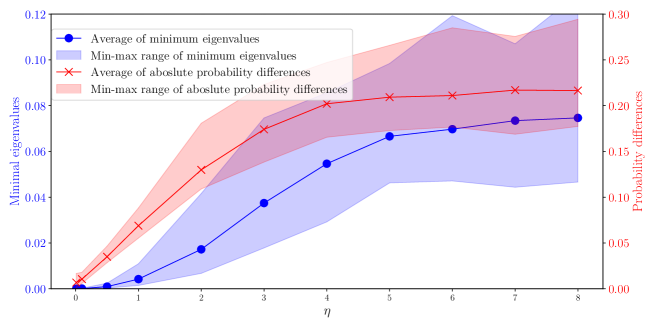
Figure 5: Minimum Eigenvalues and Absolute Probability Differences

Notes:

The plot shows averages of minimum eigenvalues (blue curve) and absolute probability differences (red curve) across 50 instances when $\eta$ changes. The ribbons gives the maximum and minimum values for either the minimum eigenvalue or the absolute probability difference corresponding to each $\eta$ value. The vertical axes are adjusted for the minimum eigenvalue or the absolute probability difference corresponding for better visulaization.

Using this proposition, we can compute $\check{\mathbf{J}}-\bm{\Gamma}\bm{\Lambda}\bm{\Gamma}^{\top}=(1-\alpha)\alpha(2p-1)^{2}>0$ in the context of Example 3.1, given that $p\neq 1/2$ and $\alpha\notin\{0,1\}$. Note that, in this simplified setting, there is no model misspecification as in (15). When $p=1/2$, $z$ becomes pure noise, and when $\alpha\in\{0,1\}$, $z$ is constant. In both cases, $z$ is uninformative. Outside of these cases, we find that AAE performs better than using only the primary data. The advantage becomes more evident if we send $p\rightarrow 0$ or $1$. In these cases, $z$ becomes more informative.

Next, we expand on this discussion, and numerically illustrate $\check{\mathbf{J}}-\bm{\Gamma}\bm{\Lambda}\bm{\Gamma}^{\top}$ under the specification of (14), and plot the results in Figure 5. Specifically, we assume that $\mathbb{P}(z=j\mid\mathbf{x})={e^{\bm{\zeta}^{\top}\mathbf{x}_{(j)}}}/\big{(}\sum_{\ell\in\mathcal{K}}e^{\bm{\zeta}^{\top}\mathbf{x}_{(\ell)}}\big{)},\,\forall j\in\mathcal{K}$, with $d=5$ and $k=2$. We vary $\eta$ across the set $\{0.01,0.1,0.5,1,2,3,4,5,6,7,8\}$, generating 50 instances for each $\eta$ value and calculating the minimum eigenvalue of $\check{\mathbf{J}}-\bm{\Gamma}\bm{\Lambda}\bm{\Gamma}^{\top}=\mathbb{E}\left[\mathbf{r}(\mathbf{x},z)\mathbf{r}(\mathbf{x},z)^{\top}\right]$. In each instance, we sample each component of $\check{\bm{\theta}}$ and $\bm{\zeta}$ from $U[-2,2]$ and each component of $\mathbf{x}$ from $U[-1,1]$, independently of one another. In Figure 5, we plot the average minimum eigenvalues across the 50 instances for each $\eta$ (blue curve) alongside the average absolute probability differences (red curve). The absolute probability difference here is defined as

$$\mathbb{E}_{\mathbf{x},z}\left[\frac{1}{k}\sum_{j\in\mathcal{K}}\left|\sigma_{j}(\mathbf{x};\bm{\beta}^{*})-g_{j}(\mathbf{x},z;\bm{\theta}^{*})\right|\right],$$

which serves as an indicator of the distance between $\sigma_{j}(\mathbf{x};\bm{\beta}^{*})$ and $g_{j}(\mathbf{x},z;\bm{\theta}^{*})$, thus intuitively reflecting the importance of $z$. Note that one can also use the KL-divergence as the metric, but we find its scale difficult to comprehend intuitively compared with the absolute probability difference.

As $\eta$ increases, the alignment between the random realizations of $y$ and $z$ also increases, signifying the growing value of the AI-generated label $z$. This effect is clearly illustrated in the red curve. The minimum eigenvalue also rises in a similar trend. Notably, the minimum eigenvalue remains consistently positive across all instances, even when $\eta=0.01$ which is very close to zero. In this case, $z$ is nearly a noise; yet in the worst case across the 50 instances, the minimum eigenvalue is still approximately $1\times 10^{-6}>0$, indicating that as long as $z$ contains some information, we can generally expect the second part of Proposition 4.4 to hold.

10 Empirical Results Evaluated Using the MSE Metric

I have checked the results in MSE and they are similar to the ones in the main body of the paper. I will add them in here later.

References

- Allenby and Rossi (2006) Allenby, Greg M, Peter E Rossi. 2006. Hierarchical bayes models. The handbook of marketing research: Uses, misuses, and future advances 418–440.
- Argyle et al. (2023) Argyle, Lisa P, Ethan C Busby, Nancy Fulda, Joshua R Gubler, Christopher Rytting, David Wingate. 2023. Out of one, many: Using language models to simulate human samples. Political Analysis 31(3) 337–351.
- Bastani et al. (2022) Bastani, Hamsa, Dennis J Zhang, Heng Zhang. 2022. Applied machine learning in operations management. Innovative Technology at the Interface of Finance and Operations: Volume I 189–222.
- Beltagy et al. (2019) Beltagy, Iz, Kyle Lo, Arman Cohan. 2019. Scibert: A pretrained language model for scientific text. arXiv preprint arXiv:1903.10676 .
- Bound et al. (2001) Bound, John, Charles Brown, Nancy Mathiowetz. 2001. Measurement error in survey data. Handbook of econometrics, vol. 5. Elsevier, 3705–3843.
- Brand et al. (2023) Brand, James, Ayelet Israeli, Donald Ngwe. 2023. Using GPT for market research. Available at SSRN 4395751 .
- Brown (2020) Brown, Tom B. 2020. Language models are few-shot learners. arXiv preprint arXiv:2005.14165 .
- Chen et al. (2023) Chen, Yiting, Tracy Xiao Liu, You Shan, Songfa Zhong. 2023. The emergence of economic rationality of gpt. Proceedings of the National Academy of Sciences 120(51) e2316205120.
- Choi et al. (2022) Choi, Tsan-Ming, Subodha Kumar, Xiaohang Yue, Hau-Ling Chan. 2022. Disruptive technologies and operations management in the industry 4.0 era and beyond. Production and Operations Management 31(1) 9–31.
- Chomsky (1956) Chomsky, Noam. 1956. Three models for the description of language. IRE Transactions on information theory 2(3) 113–124.
- Connell and Choi (2024) Connell, Paul, Jonathan H Choi. 2024. Estimating and correcting for misclassification error in empirical textual research. Available at SSRN .
- Devlin (2018) Devlin, Jacob. 2018. Bert: Pre-training of deep bidirectional transformers for language understanding. arXiv preprint arXiv:1810.04805 .
- Diederik (2014) Diederik, P Kingma. 2014. Adam: A method for stochastic optimization. (No Title) .
- Dzyabura and Jagabathula (2018) Dzyabura, Daria, Srikanth Jagabathula. 2018. Offline assortment optimization in the presence of an online channel. Management Science 64(6) 2767–2786.
- Eggers et al. (2021) Eggers, Felix, Henrik Sattler, Thorsten Teichert, Franziska Völckner. 2021. Choice-based conjoint analysis. Handbook of market research. Springer, 781–819.
- Girotra et al. (2023) Girotra, Karan, Lennart Meincke, Christian Terwiesch, Karl T Ulrich. 2023. Ideas are dimes a dozen: Large language models for idea generation in innovation. Available at SSRN 4526071 .
- Goli and Singh (2024) Goli, Ali, Amandeep Singh. 2024. Frontiers: Can large language models capture human preferences? Marketing Science .
- Green and Srinivasan (1990) Green, Paul E, Venkat Srinivasan. 1990. Conjoint analysis in marketing: new developments with implications for research and practice. Journal of marketing 54(4) 3–19.
- Green and Srinivasan (1978) Green, Paul E, Venkatachary Srinivasan. 1978. Conjoint analysis in consumer research: issues and outlook. Journal of consumer research 5(2) 103–123.
- Gui and Toubia (2023) Gui, George, Olivier Toubia. 2023. The challenge of using llms to simulate human behavior: A causal inference perspective. arXiv preprint arXiv:2312.15524 .
- Gururangan et al. (2020) Gururangan, Suchin, Ana Marasović, Swabha Swayamdipta, Kyle Lo, Iz Beltagy, Doug Downey, Noah A Smith. 2020. Don’t stop pretraining: Adapt language models to domains and tasks. arXiv preprint arXiv:2004.10964 .
- Hair Jr et al. (2019) Hair Jr, Joe, Michael Page, Niek Brunsveld. 2019. Essentials of business research methods. Routledge.
- Hinton (2015) Hinton, Geoffrey. 2015. Distilling the knowledge in a neural network. arXiv preprint arXiv:1503.02531 .
- Horton (2023) Horton, John J. 2023. Large language models as simulated economic agents: What can we learn from homo silicus? Tech. rep., National Bureau of Economic Research.
- Huang et al. (2024) Huang, Yue, Zhengqing Yuan, Yujun Zhou, Kehan Guo, Xiangqi Wang, Haomin Zhuang, Weixiang Sun, Lichao Sun, Jindong Wang, Yanfang Ye, et al. 2024. Social science meets llms: How reliable are large language models in social simulations? arXiv preprint arXiv:2410.23426 .
- HuggingFace (2024) HuggingFace. 2024. meta-llama. https://huggingface.co/meta-llama/Meta-Llama-3-8B#:~:text=Training%20Data,over%2010M%20human%2Dannotated%20examples. Accessed: 08/31/2024.
- Kessels et al. (2008) Kessels, Roselinde, Peter Goos, Martina Vandebroek. 2008. Optimal designs for conjoint experiments. Computational statistics & data analysis 52(5) 2369–2387.
- Kohli and Sukumar (1990) Kohli, Rajeev, Ramamirtham Sukumar. 1990. Heuristics for product-line design using conjoint analysis. Management Science 36(12) 1464–1478.
- Kreps et al. (2020) Kreps, Sarah, Sandip Prasad, John S. Brownstein, Yulin Hswen, Brian T. Garibaldi, Baobao Zhang, Douglas L. Kriner. 2020. Factors associated with us adults’ likelihood of accepting covid-19 vaccination. JAMA Network Open 3(10) e2025594–e2025594.
- Ludwig et al. (2024) Ludwig, Jens, Sendhil Mullainathan, Ashesh Rambachan. 2024. Large language models: An applied econometric framework. arXiv preprint arXiv:2412.07031 .
- Naveed et al. (2023) Naveed, Humza, Asad Ullah Khan, Shi Qiu, Muhammad Saqib, Saeed Anwar, Muhammad Usman, Naveed Akhtar, Nick Barnes, Ajmal Mian. 2023. A comprehensive overview of large language models. arXiv preprint arXiv:2307.06435 .
- Newey and McFadden (1994) Newey, Whitney K, Daniel McFadden. 1994. Large sample estimation and hypothesis testing. Handbook of econometrics 4 2111–2245.
- Olsen and Tomlin (2020) Olsen, Tava Lennon, Brian Tomlin. 2020. Industry 4.0: Opportunities and challenges for operations management. Manufacturing & Service Operations Management 22(1) 113–122.
- OpenAI (2023) OpenAI, R. 2023. Gpt-4 technical report. arxiv 2303.08774. View in Article 2(5).
- Pan and Yang (2009) Pan, Sinno Jialin, Qiang Yang. 2009. A survey on transfer learning. IEEE Transactions on knowledge and data engineering 22(10) 1345–1359.
- Parthasarathy et al. (2024) Parthasarathy, Venkatesh Balavadhani, Ahtsham Zafar, Aafaq Khan, Arsalan Shahid. 2024. The ultimate guide to fine-tuning llms from basics to breakthroughs: An exhaustive review of technologies, research, best practices, applied research challenges and opportunities. arXiv preprint arXiv:2408.13296 .
- Peng et al. (2024) Peng, Andrew, John Allard, Steven Heidel. 2024. Fine-tuning now available for GPT-4o. https://openai.com/index/gpt-4o-fine-tuning/. Accessed: 2024-12-15.
- Radford (2018) Radford, A. 2018. Improving language understanding by generative pre-training .
- Shane and Ulrich (2004) Shane, Scott A, Karl T Ulrich. 2004. 50th anniversary article: Technological innovation, product development, and entrepreneurship in management science. Management science 50(2) 133–144.
- Solomon (2020) Solomon, Michael R. 2020. Consumer behavior: Buying, having, and being. Pearson.
- Spencer (2019) Spencer, Vic. 2019. Choice modeling sports cars. https://github.com/spensorflow/Marketing-Analytics---Choice-Modeling-Sports-Car-Sales. Accessed: 2024-10-09.
- Sutskever (2014) Sutskever, I. 2014. Sequence to sequence learning with neural networks. arXiv preprint arXiv:1409.3215 .
- Terwiesch (2019) Terwiesch, Christian. 2019. Om forum—empirical research in operations management: From field studies to analyzing digital exhaust. Manufacturing & Service Operations Management 21(4) 713–722.
- Van der Vaart (2000) Van der Vaart, Aad W. 2000. Asymptotic statistics, vol. 3. Cambridge university press.
- Vaswani (2017) Vaswani, A. 2017. Attention is all you need. Advances in Neural Information Processing Systems .
- Wang et al. (2009) Wang, Xinfang, Jeffrey D Camm, David J Curry. 2009. A branch-and-price approach to the share-of-choice product line design problem. Management Science 55(10) 1718–1728.
- Wei et al. (2022) Wei, Jason, Xuezhi Wang, Dale Schuurmans, Maarten Bosma, Fei Xia, Ed Chi, Quoc V Le, Denny Zhou, et al. 2022. Chain-of-thought prompting elicits reasoning in large language models. Advances in neural information processing systems 35 24824–24837.
- Yang et al. (2024) Yang, Kaiqi, Hang Li, Hongzhi Wen, Tai-Quan Peng, Jiliang Tang, Hui Liu. 2024. Are large language models (llms) good social predictors? arXiv preprint arXiv:2402.12620 .
- Yao et al. (2024) Yao, Shunyu, Dian Yu, Jeffrey Zhao, Izhak Shafran, Tom Griffiths, Yuan Cao, Karthik Narasimhan. 2024. Tree of thoughts: Deliberate problem solving with large language models. Advances in Neural Information Processing Systems 36.
- Yoo et al. (2024) Yoo, Youngjin, Ola Henfridsson, Jannis Kallinikos, Robert Gregory, Gordon Burtch, Sutirtha Chatterjee, Suprateek Sarker. 2024. The next frontiers of digital innovation research. Information Systems Research .
- Zhuang et al. (2020) Zhuang, Fuzhen, Zhiyuan Qi, Keyu Duan, Dongbo Xi, Yongchun Zhu, Hengshu Zhu, Hui Xiong, Qing He. 2020. A comprehensive survey on transfer learning. Proceedings of the IEEE 109(1) 43–76.
- Ziems et al. (2024) Ziems, Caleb, William Held, Omar Shaikh, Jiaao Chen, Zhehao Zhang, Diyi Yang. 2024. Can large language models transform computational social science? Computational Linguistics 50(1) 237–291.