Orbital stability of smooth solitary waves for the modified Camassa-Holm equation

Abstract

In this paper, we explore the orbital stability of smooth solitary wave solutions to the modified Camassa-Holm equation with cubic nonlinearity. These solutions, which exist on a nonzero constant background $k$, are unique up to translation for each permissible value of $k$ and wave speed. By leveraging the Hamiltonian nature of the modified Camassa-Holm equation and employing three conserved functionals-comprising an energy and two Casimirs, we establish orbital stability through an analysis of the Vakhitov-Kolokolov condition. This stability pertains to perturbations of the momentum variable in $H^{1}(\mathbb{R})$.

1 Introduction

In this paper, we are concerned with the stability of smooth solitary waves for the following modified Camassa-Holm (mCH) equation with cubic nonlinearity

$$m_{t}+((u^{2}-u_{x}^{2})m)_{x}=0,\;\;m=u-u_{xx},$$ (1.1)

where $u(t,x)$ is a real-valued function of space-time variables $(x,t)$, and the subscripts $x$ and $t$ appended to $m$ and $u$ denote partial differentiation. The variable $m$ is deemed the “momentum variable” in the realm of peakon equations. The mCH equation (1.1) was proposed as an integrable system using a general approach of the tri-Hamiltonian duality by Fuchssteiner [9] and Olver and Rosenau [35]. Also, Equation (1.1) is integrable in the sense that it has a bi-Hamiltonian structure [9, 35, 36] and it admits a Lax pair [36]. Later, the generalization of (1.1) with a dispersive term given below in (1.2) was obtained by Qiao [37] from the two-dimensional Euler equations with the variable $u$ representing the velocity of the fluid. Qiao also obtained the bi-Hamiltonian structure together with the Lax pair. Furthermore, it is shown in [10] that Equation (1.2) arises from an intrinsic invariant planar curve flow in Euclidean geometry.

Equation (1.1) admits a variety of solutions on the whole line, for both the cases of zero and nonzero backgrounds. More specifically, (1.1) admits peaked solitary waves (peakons) [10], which are asymptotically going to zero, whereas the smooth multisoliton solutions [16, 30] tend to a nonzero constant as $x\to\pm\infty$. Orbital stability of the single peakons for the mCH equation (1.1) was obtained in [38] using an approach similar to what was done in [2, 26] for the Camassa-Holm and Degasperis-Procesi one-peakon solutions. As for the train of peakons of the mCH equation (1.1), their orbital stability was obtained in [27] by using an energy argument and combining the method of the orbital stability of a single peakon with the monotonicity of the local energy norm [29, 18].

In [25], Li, Liu, and Zhu investigated the stability of smooth solitary-wave solutions for the mCH equation with a linear dispersion term, given by

$$m_{t}+((u^{2}-u_{x}^{2})m)_{x}+\gamma u_{x}=0,\;\;\;m=u-u_{xx},$$ (1.2)

where $\gamma$ is a positive constant. Unlike the mCH equation (1.1), which does not admit smooth traveling wave solutions with vanishing boundary conditions, Equation (1.2) admits smooth soliton solutions that vanish at infinity [31, 20]. By constructing conserved quantities in terms of the momentum variable $m$, it is shown in [25] that the smooth soliton for Equation (1.2) is orbitally stable to perturbations to $m$ in $H^{1}(\mathbb{R})$. As discussed in detail in [25, Section 1], it would be challenging to apply the framework developed by Grillakis, Shatah, and Strauss in [11] or the methods used for the Camassa-Holm equation in [3]. This is due to the cubic nonlinearity of the mCH equation, which causes the integrands of the conserved functionals to be quartic. Similar difficulties arise in establishing the orbital stability of smooth solitons of the Degasperis-Procesi equation (see the discussions in the introductions of [22, 23, 24]). Therefore, an approach following entirely the method outlined in [11] based on the Hamiltonian structure in the variable $u$ with invertible Hamiltonian operator does not seem to be the best of choices for the mCH equation (1.1).

Inspired by the works in [14, 19, 7], we aim to study the stability of smooth solitary wave solutions of the mCH equation (1.1) using a Hamiltonian structure, written in the variable $m$, that admits Casimirs. Our general approach is as follows. First, we establish the existence of smooth solitary waves for (1.1) under nonzero boundary conditions. We then demonstrate that such waves can be considered as critical points of an appropriate action functional expressed in the variable $m$, constructed out of a linear combination of the Hamiltonian and the Casimirs, similarly as done for the $b$-family in [14, 19, 21] and for the Novikov equation in [7] (with the Casimirs for the Novikov equation given in [15, Section 3]). Note that the $b$-family is a peakon equation that has a free parameter denoted by $b$ [4, 6], which includes two integrable cases: the Camassa–Holm equation [1] ($b=2$) and the Degasperis–Procesi equation [5] ($b=3$). Novikov proposed the integrable Novikov peakon equation in [32], and it is regarded as a generalization of the Camassa-Holm equation that accounts for cubic nonlinearities.

Next, we aim to determine conditions that ensure such solitary waves are constrained local extrema of the Hessian of the associated action functional. This strategy is in line with the Energy-Casimir method [13], except that in the next step, one finds that the Hessian operator has negative spectrum. Nevertheless, after establishing the spectral properties of the Hessian operator, we show that these waves are orbitally stable in the constrained space, provided that a so-called Vakhitov-Kolokolov condition [39] is satisfied. Finally, we verify that the Vakhitov-Kolokolov condition always holds, indicating that the smooth solitary wave solutions of the mCH equation (1.1) are orbitally stable, a consequence of the general stability result established in [11].

Notice that there exist no smooth solitary waves for the mCH equation (1.1) with vanishing boundary condition. Therefore, we consider the solutions of (1.1) on a nonzero constant background with $m(t,x)\rightarrow k$ as $x\rightarrow\pm\infty$. Moreover, for fixed $k>0$, we consider the class of functions in the set

$$X_{k}:=\{m-k\in H^{1}(\mathbb{R}):m(x)>0,\,x\in\mathbb{R}\}.$$ (1.3)

The three conserved integrals we are using to construct the Lyapunov functional are given by

$$F_{1}(m)=\int_{\mathbb{R}}(m-k)\,dx$$ (1.4)

$$F_{2}(m)=\int_{\mathbb{R}}\left(\frac{1}{m}-\frac{1}{k}\right)\,dx$$ (1.5)

and

$$F_{3}(m)=\int_{\mathbb{R}}\left(\frac{m_{x}^{2}}{m^{5}}+\frac{1}{4m^{3}}-\frac{1}{4k^{3}}\right)\,dx.$$ (1.6)

The fact that $F_{1}$ is constant is evident. The conserved integrals $F_{2}$ and $F_{3}$ were derived in [30] using a Bäcklund transformation. However, since it is not immediately apparent that $F_{2}$ and $F_{3}$ are conserved, we verify this fact explicitly in Section 2.2.

The equation (1.1) can be written in Hamitonian form with energy given by $F_{1}$ above as [17, Section 2]

$$m_{t}={\mathcal{J}}\frac{\delta F_{1}}{\delta m},\;\;{\mathcal{J}}\equiv\partial_{x}m\partial_{x}^{-1}m(\partial_{x}^{2}-1)^{-1}\partial_{x}m\partial_{x}^{-1}m\partial_{x}.$$ (1.7)

In Section 2.2, we show that $F_{2}$ and $F_{3}$ are Casimirs for the Hamiltonian system described above, thus providing an alternative proof that $F_{2}$ and $F_{3}$ are conserved quantities. Also, by doing so, we show that the Lyapunov functional is obtained by taking the energy functional and a linear combination of the Casimirs, as done in [14, 19, 7] for smooth solutions to the $b$-family and the Novikov equations.

The main result of this article is given in the following theorem.

Theorem 1.1.

For fixed $c>0$, and $k\in(\frac{\sqrt{c}}{3},\frac{\sqrt{3c}}{3})$, there exists a unique smooth solitary wave $m(t,x)=\mu(x-ct)$ of the mCH equation (1.1). This solitay wave $\mu(x-ct)$ is orbitally stable in the space $X_{k}$ defined in (1.3), namely, if for every $\varepsilon>0$ there exists $\delta=\delta(\varepsilon)>0$ such that for every $m_{0}\in X_{k}$ satisfying $\|m_{0}-\mu(\cdot)\|<\delta$, there exists a unique solution $m\in C^{0}(\mathbb{R},X_{k})$ of the mCH equation (1.1) with the initial datum $m(0,\cdot)=m_{0}$ and the maximal existence time $T>0$ satisfying

$$\inf_{r\in\mathbb{R}}\left\{\|m(t,\cdot)-\mu(\cdot+r)\|<\varepsilon,t\in[0,T)\right\}.$$

Remark 1.1.

Note that

$$\|m\|^{2}_{H^{1}}=\int_{\mathbb{R}}(m^{2}+m_{x}^{2})dx=\int_{\mathbb{R}}(u^{2}+3u_{x}^{2}+3u_{xx}^{2}+u_{xxx}^{2})\,dx$$

which is equivalent to the $H^{3}(\mathbb{R})$ norm on $u$. Thus it follows from Theorem 1.1 that if $u(t,x)=\phi(x-ct)$ is the traveling wave solution of Equation (1.1) with $\phi\in Y_{k}$ given by

$$\begin{split}Y_{k}:=\{u-k\in H^{3}(\mathbb{R}):u-u_{xx}>0,x\in\mathbb{R}\}.\end{split}$$

Then, by Theorem 1.1, such wave is orbitally stable in $Y_{k}$ in the $H^{3}(\mathbb{R})$ norm.

Remark 1.2.

The existence and uniqueness of the smooth solitary wave in Theorem 1.1 will be established in Lemma 3.1.

Remark 1.3.

The solutions studied in [25] for Equation (1.2) are on a zero background, and thus are not related to the solitary wave with non-zero background for the mCH equation (1.2) with $\gamma=0$ (i.e. equation (1.1)). Hence, our results are not obtainable by simply taking the limit as $\gamma\to 0$.

Remark 1.4.

Equation (1.2) possesses, among others, the following two conserved integrals [30], which were used in [25] to prove the orbital stability of the smooth solitary wave solutions when $\gamma\neq 0$:

$$\begin{split}E(m)=\int_{\mathbb{R}}\left(M-\sqrt{\frac{\gamma}{2}}\right)dx,\ \ F(m)=\int_{\mathbb{R}}\left(\frac{m_{x}^{2}}{2M^{5}}-\frac{1}{\gamma M}+\sqrt{2}\gamma^{-\frac{3}{2}}\right)dx,\end{split}$$

where $M=\sqrt{m^{2}+\frac{\gamma}{2}}$. While the expression for $F$ above is similar to the function $F_{3}$ from (1.6) used in the case $\gamma=0$, the limit $\gamma\to 0$ cannot be performed on $F$. This suggests that $F_{3}$ is a conserved functional does not arise as a reduction of a functional from the case $\gamma>0$.

The remainder of this paper is organized as follows. In Section 2, we provide a brief review of the well-posedness of the mCH equation (1.1) and demonstrate that the integrals defined in (1.5) and (1.6) are conserved over time. We achieve this in two ways: first, by directly computing their time derivatives, and second, by showing that they are Casimirs for the Hamiltonian operator $\mathcal{J}$ defined in (1.7). In Section 3, we examine the existence and fundamental properties of smooth solitary wave solutions of the mCH equation (1.1). Specifically, we show that these solitary waves can be viewed as critical points of an explicit action functional $\Lambda$, and we then provide analytic spectral properties of the operator $\mathcal{L}=\frac{\delta^{2}\Lambda}{\delta^{2}m}$ evaluated at these solitary waves. Section 4 is devoted to the analysis of orbital stability. By demonstrating that the Vakhitov-Kolokolov condition is always satisfied, we then complete the proof of Theorem 1.1.

2 Well-posedness and conservation laws

In this section, we first recall the well-posedness results for the Cauchy problem of the mCH equation (1.1), and then present a proof that the conserved integrals defined in (1.5) and (1.6) are conserved over time. It is assumed that the solution $m$ satisfies the properties necessary for the existence of these conserved integrals.

2.1 Well-posedness

We consider the Cauchy problem of the mCH equation on the real line, that is,

$$\left\{\begin{array}[]{l}m_{t}+\left((u^{2}-u_{x}^{2})m\right)_{x}=0,\,\,\,\,m=u-u_{xx},\\ \\ u(0,x)=u_{0}(x),x\in\mathbb{R}.\end{array}\right.$$ (2.1)

The following local well-posedness result and the properties of solutions on the line were established in [10]

Proposition 2.1.

Let $u_{0}\in H^{s}(\mathbb{R})$ with $s>\frac{5}{2}$. Then there exists a time $T>0$ such that the initial value problem (2.1) has a unique solution $u\in C([0,T),H^{s}(\mathbb{R}))\cap C^{1}([0,T),H^{s-1}(\mathbb{R}))$. Moreover, the solution $u$ depends continuously on the initial data, and if $m_{0}=(1-\partial_{x}^{2})u_{0}$ does not change sign, then $m(t,x)$ will not change sign for any $t\in[0,T)$. More precisely, if $m_{0}(x)>0$, then the corresponding solution $u(t,x)$ is positive and satisfies $|u_{x}(t,x)|\leq u(t,x)$ for $(t,x)\in[0,T)\times\mathbb{R}$.

2.2 Proof that the functionals $F_{2}$ and $F_{3}$ are conserved

We first do this by a direct computation. It follows from (1.1) that

$$m_{t}=-[(u^{2}-u_{x}^{2})m_{x}+2m^{2}u_{x}],\ \ m_{tx}=-[(u^{2}-u_{x}^{2})m_{xx}+6u_{x}mm_{x}+2m^{2}(u-m)],$$ (2.2)

A straightforward calculation shows that

$$\frac{d}{dt}F_{2}(m(t)) = \frac{d}{dt}\int_{\mathbb{R}}\left(\frac{1}{m}-\frac{1}{k}\right)dx$$

$$= \int_{\mathbb{R}}\left[2u_{x}+\frac{(u^{2}-u_{x}^{2})m_{x}}{m^{2}}\right]dx$$

$$= -\int_{\mathbb{R}}(u^{2}-u_{x}^{2})\left(\frac{1}{m}\right)_{x}dx$$

$$= \int_{\mathbb{R}}\frac{(u^{2}-u_{x}^{2})_{x}}{m}dx$$

$$= \int_{\mathbb{R}}2u_{x}dx=0.$$

Similary, we have

$$\frac{d}{dt}F_{3}(m(t)) = \frac{d}{dt}\int_{\mathbb{R}}\frac{m_{x}^{2}}{m^{5}}dx+\frac{d}{dt}\int_{\mathbb{R}}\frac{1}{4m^{3}}dx$$

$$= I_{1}+I_{2}.$$

In view of (2.2), and integrating by parts several times leads to

$$I_{1} = \frac{d}{dt}\int_{\mathbb{R}}\frac{m_{x}^{2}}{m^{5}}dx$$

$$= \int_{\mathbb{R}}\left(\frac{2m_{x}m_{xt}}{m^{5}}-\frac{5m_{x}^{2}m_{t}}{m^{6}}\right)dx$$

$$= \int_{\mathbb{R}}\left(\frac{-2m_{x}[(u^{2}-u_{x}^{2})m_{xx}+6mm_{x}u_{x}+2m^{2}(u-m)]}{m^{5}}+\frac{5m_{x}^{2}[(u^{2}-u_{x}^{2})m_{x}+2m^{2}u_{x}]}{m^{6}}\right)dx$$

$$= \int_{\mathbb{R}}\left(\left[\frac{-m_{x}^{2}(u^{2}-u_{x}^{2})}{m^{5}}\right]_{x}-\frac{4m_{x}(u-m)}{m^{3}}\right)dx$$

$$= -\int_{\mathbb{R}}\left.\frac{4m_{x}(u-m)}{m^{3}}\right.dx,$$

and

$$I_{2} = \frac{d}{dt}\int_{\mathbb{R}}\frac{1}{4m^{3}}dx$$

$$= \int_{\mathbb{R}}\frac{3}{4m^{4}}[(u^{2}-u_{x}^{2})m]_{x}dx$$

$$= \int_{\mathbb{R}}\left(\frac{3}{4}\left[\frac{u^{2}-u_{x}^{2}}{m^{3}}\right]_{x}+\frac{3(u^{2}-u_{x}^{2})m_{x}}{m^{4}}\right)dx$$

$$= -\int_{\mathbb{R}}(u^{2}-u_{x}^{2})\left(\frac{1}{m^{3}}\right)_{x}dx$$

$$= \int_{\mathbb{R}}\left(\frac{(u^{2}-u_{x}^{2})_{x}}{m^{3}}-\left[\frac{u^{2}-u_{x}^{2}}{m^{3}}\right]_{x}\right)dx$$

$$= \int_{\mathbb{R}}\left(\frac{2u_{x}}{m^{2}}\right)dx.$$

Thus, we obtain

$$I_{1}+I_{2} = \int_{\mathbb{R}}\left(-\frac{4m_{x}(u-m)}{m^{3}}+\frac{2u_{x}}{m^{2}}\right)dx$$

$$= \int_{\mathbb{R}}\left(\frac{-4um_{x}}{m^{3}}-4\left(\frac{1}{m}\right)_{x}+\frac{2u_{x}}{m^{2}}\right)dx$$

$$= \int_{\mathbb{R}}\left(\frac{-4um_{x}}{m^{3}}+\frac{2u_{x}}{m^{2}}\right)dx$$

$$= \int_{\mathbb{R}}\left(\frac{2u}{m^{2}}\right)_{x}dx=0.$$

Consequently, it yields that $\frac{d}{dt}F_{3}(m(t))=0$.

Here we prove that $F_{2}$ and $F_{3}$ given in (1.5) and (1.6) are Casimirs for the Hamiltonian operator $\mathcal{J}$ in (1.7), thus providing an alternative proof that they are conserved. The computation below is similar to what is done in [19, Appendix A] for conserved quantities of the $b$-family. Suppose that $\mathcal{J}f=0$, with $\mathcal{J}$ given in (1.7). Then we have

$$\begin{split}\mathcal{J}f=\partial_{x}m\partial_{x}^{-1}m(\partial_{x}^{2}-1)^{-1}\partial_{x}m\partial_{x}^{-1}m\partial_{x}f=0.\end{split}$$ (2.3)

In order to find $f$, we first use the easily found fact that the kernel of $\partial_{x}m\partial_{x}^{-1}$ is one dimensional and given by

$$\begin{split}\ker\left(\partial_{x}m\partial_{x}^{-1}m\right)=\left\{\sigma\frac{m_{x}}{m^{3}}:\sigma\in\mathbb{R}\right\}.\end{split}$$ (2.4)

Using (2.4), we can write (2.3) in the equivalent form

$$\begin{split}(\partial_{x}^{2}-1)^{-1}\partial_{x}m\partial_{x}^{-1}m\partial_{x}f=k_{1}\frac{m_{x}}{m^{3}},\end{split}$$ (2.5)

for some free constant $k_{1}$. It can be computed in a straightforward manner that

$$\begin{split}{m^{-1}\partial_{x}m^{-1}\partial_{x}^{-1}(\partial_{x}^{2}-1)\left(k_{1}\frac{m_{x}}{m^{3}}\right)=-\frac{1}{2}\left(k_{1}\frac{\delta F_{3}}{\delta m}+k_{2}\frac{\delta F_{2}}{\delta m}\right)_{x},}\end{split}$$ (2.6)

for another free constant $k_{2}$. As a consequence of (2.6), we have that

$$\begin{split}f=k_{1}\frac{\delta F_{3}}{\delta m}+k_{2}\frac{\delta F_{2}}{\delta m}\end{split}$$ (2.7)

satisfies (2.5) for arbitrary $k_{1}$ and $k_{2}$. Thus, the functionals $F_{2}$ and $F_{3}$ are Casimirs for the operator $\mathcal{J}$. The functional $F_{2}$ was identified as a Casimir in [17, Section 3.2]. More precisely, the function $f$ given in (2.7) solves (2.5) for the correct choice of the constant of integration when applying $\partial_{x}^{-1}$ and $(1-\partial_{x}^{2})^{-1}$. This can be achieved by carefully selecting appropriate limits of integration when defining these operators, along with the corresponding boundary conditions. For instance, see [28] (particularly Equation 2.2 therein), which addresses Casimirs in the context of nonlocal Hamiltonian operators, and also [12, Section 2]. Furthermore, the implications of having a nonlocal Hamiltonian operator are discussed in [17, Remark 2.5] in the context of the mCH equation (1.1). For additional discussions on nonlocal operators in the context of symmetries, refer to [34, 33].

3 Smooth solitary wave solutions

In this section, we employ phase plane analysis to establish the existence of a one-parameter family of smooth solitary wave solutions for the mCH equation on a nonzero constant background. We then show that these solutions can be characterized variationally as the critical points of an action functional $\Lambda$. This functional is composed of a linear combination of the energy $F_{1}$ (1.4) and the Casimirs $F_{2}$ (1.5) and $F_{3}$ (1.6). Finally, we derive the spectral properties of the Hessian operator $\mathcal{L}$ associated with the action functional $\Lambda$.

3.1 Existence of smooth solitary wave solutions

We consider the traveling wave solutions of (1.1) of the form $u(t,x)=\phi(\xi)$, $\xi=x-ct$. After integration, we find that the profile $\phi$ satisfies the ODE

$$(\phi-\phi_{\xi\xi})(\phi_{\xi}^{2}-\phi^{2}+c)=a,$$ (3.1)

where $a$ is an integration constant.

The following lemma describes the family of solitary waves parameterized by the arbitrary nonzero background parameter $k>0$.

Lemma 3.1.

For fixed $c>0$, there exists a family of smooth solitary waves with $\phi\in C^{\infty}(\mathbb{R})$ satisfying $\phi(\xi)\rightarrow k$ as $|\xi|\rightarrow\infty$ if and only if $k\in(\frac{\sqrt{c}}{3},\frac{\sqrt{3c}}{3})$. Moreover,

$$k<\phi(\xi)\leq\sup_{\xi\in\mathbb{R}}{(\phi)}=\sqrt{2(c-k^{2})}-k,\ \ \mu=\phi-\phi_{\xi\xi}>0,\ \ \xi\in\mathbb{R}.$$

Proof.

Equation (3.1) can be rewritten as the following two-dimensional dynamical system

$$\left\{\begin{array}[]{l}\phi_{\xi}=\psi,\\ \\ (c+\psi^{2}-\phi^{2})\psi_{\xi}=\phi(c+\psi^{2}-\phi^{2})-a.\end{array}\right.$$ (3.2)

Another invariant of (3.1) can be obtained by multiplying the equation by $\phi_{\xi}$, performing an integration, and use the definition of $\psi$ given in (3.2), which yields

$$(\phi^{2}-\psi^{2})^{2}-2c(\phi^{2}-\psi^{2})+4a\phi=E,$$ (3.3)

where $E$ is another integral constant.

A smooth solitary wave profile satisfying $\phi(\xi)\rightarrow k$ as $|\xi|\rightarrow\infty$ correspond to a homoclinic orbit to the equilibrium point $(\phi,\psi)=(k,0)$ of system (3.2). Taking the limit as $|\xi|\rightarrow\infty$ in (3.1) and (3.3) yields the relations

$$a=k(c-k^{2}),\ \ E=k^{2}(2c-3k^{2}).$$ (3.4)

After substituting (3.4) into (3.3), it is found that a homoclinic orbit to $(k,0)$ corresponds a bounded connected component of the level curve, denoted by

$$\begin{split}\Gamma:(\phi^{2}-\psi^{2})^{2}-2c(\phi^{2}-\psi^{2})+4k(c-k^{2})\phi=k^{2}(2c-3k^{2}),\end{split}$$

which is equivalent to

$$\Gamma:(\phi^{2}-\psi^{2}-c)^{2}=(c-k^{2})(c+3k^{2}-4k\phi).$$ (3.5)

In order to have a homoclinic orbit to $(k,0)$, the curve $\Gamma$ must intersect the $\phi$ axis at least one point different from $(k,0)$. Setting $\psi=0$ and assuming that $\phi\neq k$, we find that the equation defining $\Gamma$ is equivalent to

$$(\phi+k)^{2}=2(c-k^{2})\Rightarrow c>k^{2},\ \ \phi_{1,2}=\pm\sqrt{2(c-k^{2})}-k.$$ (3.6)

On the other hand, it follows from (3.5) that

$$\psi^{2}=\phi^{2}-c\pm\sqrt{(c-k^{2})(c+3k^{2}-4k\phi)}.$$ (3.7)

In view of the fact that $c>k^{2}$, in order for (3.7) to admit $(k,0)$ as a solution, one must choose the “$+$” branch and consider the curve defined by

$$\psi^{2}=\phi^{2}-c+\sqrt{(c-k^{2})(c+3k^{2}-4k\phi)}.$$ (3.8)

The RHS of (3.8) has at most three zeros (not counting multiplicity): $\phi=k$ and, possibly, $\phi=\phi_{i},i=1,2$. It inherits a zero at $\phi=\phi_{i}$ from the solutions of (3.6), and its value is distinct from $\phi=k$, if and only if $\phi_{i}^{2}-c<0$. As a consequence, Equation (3.8) does not admit $(\phi_{2},0)$ as a solution since a simple calculation shows that

$$\phi_{2}^{2}-c=c-k^{2}+2k\sqrt{2(c-k^{2})}>0.$$

The RHS of equation (3.8) thus has $\phi=k$ as a double zero and $\phi=\phi_{1}$ as a simple one if $\phi_{1}^{2}<c$. Furthermore, for equation (3.8) to define a close curve that includes the fixed point $(k,0)$ and $(\phi_{1},0)$, one needs the RHS of the equation to be positive on the open interval between $k$ and $\phi_{1}$. Since the RHS is positive for $\phi<0$, has a double zero at $\phi=k$, and a distinct simple zero at $\phi=\phi_{1}$ (if $\phi_{1}^{2}<c$), Equation (3.8) defines a closed curve in the $\phi-\psi$ plane if and only if $\phi=\phi_{1}$ is a zero of RHS and $\phi_{1}>k$. So the conditions for (3.8) to define a closed curve with the points $(k,0)$ and $(\phi_{1},0)$ in it are

$$\begin{split}\phi_{1}^{2}-c<0\text{ and }\phi_{1}>k,\end{split}$$ (3.9)

which leads to the conditions $k^{2}\in\left(\frac{c}{9},\frac{c}{3}\right)$.

Thus, in that case, (3.8) defines the homoclinic orbit

$$\left\{(\phi,\psi):\psi^{2}=\phi^{2}-c+\sqrt{(c-k^{2})(c+3k^{2}-4k\phi)},\phi>k\right\}$$

and the equilibrium point $(k,0)$.

Finally, it follows from (3.8) and the condition given in (3.9) on the maximum value $\phi_{1}$ of the wave that

$$\phi^{2}-\phi_{\xi}^{2}-c=\phi^{2}-\psi^{2}-c<0.$$ (3.10)

By (3.1), we can derive that $\phi-\phi_{\xi\xi}>0$ since $a=k(c-k^{2})>0$. The statement about the supremum of $\phi$ made in the lemma is a consequence of the formula for $\phi_{1}$ made in (3.6). ∎

Remark 3.1.

In the limiting case $k\rightarrow\frac{\sqrt{3c}}{3}$, the level curve $\Gamma$ will intersect the $\phi$ axis at the saddle point $(k,0)$. This implies that there exists no smooth solitary wave. In the limiting case $k\rightarrow\frac{\sqrt{c}}{3}$, $\phi^{2}-\phi_{\xi}^{2}-c$ approaches zero at the location of the maximum value of the solitary wave since $\phi_{1}\to c^{-}$. It then follows from (3.1) that $\phi_{\xi\xi}\to-\infty$ at that same location. Thus, the solitary wave is no longer smooth.

Remark 3.2.

Let $\phi:=k+(1-\partial_{x}^{2})^{-1}(\mu-k)$, then the following relation between $\mu$ and $\phi$ is obtained obtained from (3.1), (3.4), and (3.8):

$$\mu=k\sqrt{\frac{c-k^{2}}{c+3k^{2}-4k\phi}}.$$ (3.11)

Remark 3.3.

Note that $k<\phi(\xi)\leq\phi_{1}=\sqrt{2(c-k^{2})}-k$ (see (3.6)). It follows from (3.11) that

$$k<\mu(\xi)\leq M_{c,k},$$

where $M_{c,k}=\frac{k\sqrt{c-k^{2}}}{2\sqrt{2}k-\sqrt{c-k^{2}}}$. Hence, $M_{c,k}\rightarrow\infty$ as $k\rightarrow\frac{\sqrt{c}}{3}$.

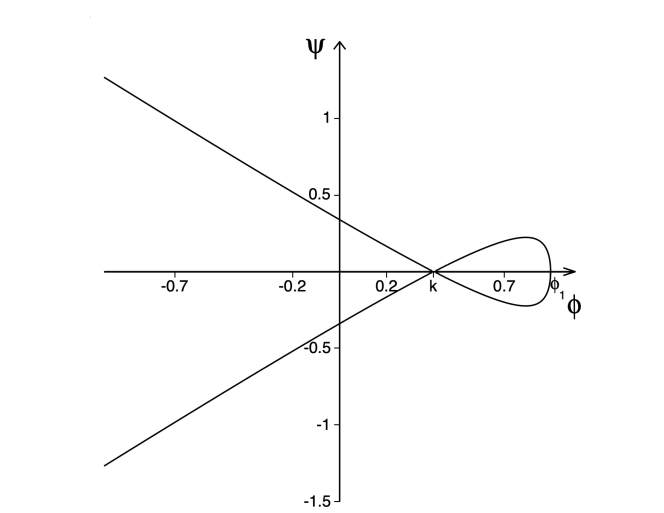
Figure 1: Graph of the curve defined by Equation (3.8) in the case $k=0.4$ and $c=1$, corresponding to $\phi_{1}=0.896148140$.

3.2 Variational characterization

We now show that the profile equations (3.1) and (3.3) satisfied by the smooth solitary waves $\mu(\textperiodcentered;k)$ correspond to the Euler-Lagrange equation of the action functional

$$\Lambda(m):=F_{3}(m)+\omega_{1}F_{1}(m)+\omega_{2}F_{2}(m),\ \ m\in X_{k},$$ (3.12)

where $m=u-u_{xx}$, and the conserved quantities $F_{1},F_{2}$ and $F_{3}$ are given in (1.4), (1.5) and (1.6). The following lemma states that the variational characterization is possible if and only if the Lagrange multipliers $\omega_{1}$ and $\omega_{2}$ are uniquely related to parameters of Eqs.(3.1) and (3.3).

Lemma 3.2.

(Variational characterization) For any fixed $c>0$ and $k\in(\frac{\sqrt{c}}{3},\frac{\sqrt{3c}}{3})$, a critical point $\mu$ of the action functional $\Lambda$ coincides with the solitary wave solution $\mu=\phi-\phi_{\xi\xi}\in C^{\infty}(\mathbb{R})$, where $\phi$ is the unique positive solitary wave solution for the mCH equation (1.1), if and only if

$$\omega_{1}=\frac{c-9k^{2}}{4k^{4}(c-k^{2})},\quad\omega_{2}=-\frac{c+3k^{2}}{2k^{2}(c-k^{2})}.$$ (3.13)

Proof.

Let $\mu\in X_{k}$ be a critical point of $\Lambda$. After straightforward simplifications, the equation $\frac{\delta\Lambda}{\delta m}(\mu)=0$ gives the following differential equation

$$\omega_{1}-\frac{\omega_{2}}{\mu^{2}}-\frac{2\mu_{\xi\xi}}{\mu^{5}}+\frac{5\mu_{\xi}^{2}}{\mu^{6}}-\frac{3}{4\mu^{4}}=0.$$ (3.14)

We want to show that the above differential equation (3.14) is satisfied whenever $\mu$ satisfies the profile equation (3.1) and (3.3), only if the Lagrange multipliers $\omega_{1}$ and $\omega_{2}$ are chosen as stated in (3.13).

Using (3.1) and (3.3) we have

$$\mu=\phi-\phi_{\xi\xi}=\frac{a}{\phi_{\xi}^{2}-\phi^{2}+c},\ \ \phi^{2}-\phi_{\xi}^{2}-c=-\sqrt{c^{2}+E-4a\phi},$$ (3.15)

since $\phi^{2}-\phi_{\xi}^{2}-c$ is negative (see (3.8)).

Thus, a direct calculation shows that

$$\mu_{\xi}=\frac{2a\phi_{\xi}\mu}{(\phi^{2}-\phi_{\xi}^{2}-c)^{2}}=2a^{-1}\phi_{\xi}\mu^{3},$$ (3.16)

and

$$\mu_{\xi\xi}=2a^{-1}\phi_{\xi\xi}\mu^{3}+12a^{-2}\phi_{\xi}^{2}\mu^{5}.$$ (3.17)

Substituting (3.15), (3.16) and (3.17) into (3.14) yields

$$\begin{split}\omega_{1}-a^{-2}\omega_{2}(c^{2}+E-4a\phi)+2a^{-3}(c^{2}+E)\phi+4a^{-2}c-\frac{3}{4}a^{-4}(c^{2}+E)^{2}=0.\end{split}$$

By grouping the constant terms and $\phi$ separately, this immediately gives the unique choice for Lagrange multipliers

$$\omega_{1}=-4a^{-2}c+\frac{1}{4}a^{-4}(c^{2}+E)^{2},\quad\omega_{2}=-\frac{1}{2}a^{-2}(c^{2}+E).$$ (3.18)

Finally, substituting (3.4) into (3.18) gives (3.13). ∎

Our next goal is to characterize the property of the critical point $\mu$ as a local minimum, maximum or a saddle point. To this end, note that $\mu$ is uniformly bounded below by $k>0$ by Remark 3.3, we have $\mu+\widetilde{m}\in X_{k}$ if $\|\widetilde{m}\|_{H^{1}(\mathbb{R})}$ is sufficiently small.

The following result describes the second-order variation of the action functional $\Lambda$. In what follows, $<.,.>$ denotes the standard inner product in $L^{2}(\mathbb{R})$ space, and $\omega_{1},\omega_{2}$ are selected by Lemma 3.2.

Corollary 3.1.

There exists a sufficiently small $\varepsilon>0$ such that for every $\widetilde{m}\in H^{1}(\mathbb{R})$ satisfying $\|\widetilde{m}\|_{H^{1}(\mathbb{R})}\leq\varepsilon$, we have

$$\Lambda(\mu+\widetilde{m})-\Lambda(\mu)=\frac{1}{2}<\mathcal{L}\widetilde{m},\widetilde{m}>+R(\widetilde{m}),$$ (3.19)

where $\mathcal{L}:=\frac{\delta^{2}\Lambda}{\delta^{2}m}$ is given by

$$\mathcal{L}=-\partial_{\xi}\mu^{-5}\partial_{\xi}+5\mu_{\xi\xi}\mu^{-6}-15\mu_{\xi}^{2}\mu^{-7}+\frac{3}{2}\mu^{-5}-\frac{c+3k^{2}}{2k^{2}(c-k^{2})}\mu^{-3},$$ (3.20)

and $\|R(\widetilde{m})\|_{H^{1}}\leq C_{0}\|\widetilde{m}\|^{3}_{H^{1}}$ for a positive constant $C_{0}$ independent of $\widetilde{m}$.

Proof.

The expression for $\mathcal{L}$ can be obtained by using the straightforward Taylor expansion of $\Lambda(\mu+\widetilde{m})-\Lambda(\mu)$. Since $\mu$ are strictly positive, bounded, and smooth on $\mathbb{R}$ by Lemma 3.1 and Remark 3.3, we conclude that all the coefficients of the Sturm-Liouville operator $\mathcal{L}$ are smooth and bounded.

On the other hand, $R(\widetilde{m})$ can be computed by using the Taylor expansion of the functionals $F_{2}(m)$ and $F_{3}(m)$ at $m=\mu$. Note that the leading order term in $R(\widetilde{m})$ is cubic and the Sobolev space $H^{1}(\mathbb{R})$ forms a Banach algebra with respect to multiplication, so $\|R(\widetilde{m})\|_{H^{1}}\leq C_{0}\|\widetilde{m}\|^{3}_{H^{1}}$ follows from the Taylor expansion of $F_{2}(m)$ and $F_{3}(m)$ and the smallness of $\|\widetilde{m}\|_{H^{1}}$.

∎

3.3 Spectral properties of $\mathcal{L}$

The goal of this subsection is to show that the Hessian operator $\mathcal{L}$ of the action functional $\Lambda$ defined by (3.19) and (3.20) has exactly one simple negative eigenvalue and a simple zero eigenvalue isolated from the rest of the spectrum.

Note that $c+\phi_{\xi}^{2}-\phi^{2}>0$, making the Liouville substitution

$$\begin{split}z=\int_{0}^{\xi}\frac{1}{(c+\phi_{x}^{2}-\phi^{2})^{\frac{5}{2}}}dx,\quad\omega(z)=(c+\phi_{\xi}^{2}-\phi^{2})^{\frac{5}{4}}\upsilon(\xi),\end{split}$$ (3.21)

transforms the spectral equation $\mathcal{L}\upsilon=\lambda\upsilon$ into

$$\mathcal{A}\omega(z)=\left(-a^{-5}\partial_{z}^{2}+\frac{3}{2}\mu^{-5}-\frac{c+3k^{2}}{2k^{2}(c-k^{2})}\mu^{-3}+q(z)\right)\omega(z)=\lambda\omega(z),$$ (3.22)

where

$$q(z)=5\mu_{\xi\xi}\mu^{-6}-15\mu_{\xi}^{2}\mu^{-7}+\frac{5}{2}a^{-1}\mu^{-3}\phi_{\xi\xi}-\frac{35}{4}a^{-2}\mu^{-1}\phi_{\xi}.$$

The transformation defined in (3.21) does not alter the spectrum. This is a consequence of the fact that the expression $c+\phi_{\xi}^{2}-\phi^{2}$ limits to $c-k^{2}>0$ as $|\xi|\to\infty$ and, by (3.10), it is strictly positive. Thus, the expression multiplying $\upsilon(x)$ in (3.21) is uniformly bounded away from zero, and the spectra of $\mathcal{A}$ and $\mathcal{L}$ are the same.

Both $\mathcal{L}$ and $\mathcal{A}$ are defined in $H^{2}(\mathbb{R})\subset H^{1}(\mathbb{R})$ dense in $L^{2}(\mathbb{R})$ and it can be verified that all the coefficients of both $\mathcal{L}$ and $\mathcal{A}$ are smooth and bounded. Thus they can be extended as unbounded self-adjoint Sturm-Liouville operators in $L^{2}(\mathbb{R})$. The following proposition gives the spectral properties of the linear operator $\mathcal{L}$.

Proposition 3.1.

(1) The spectrum is real, $\sigma(\mathcal{L})\subset\mathbb{R}$;

(2) 0 is a simple isolated eigenvalue of $\mathcal{L}$ with $\mu_{\xi}$ as its eigenfunction;

(3) There exists $\delta>0$ such that $\sigma(\mathcal{L})$ in $(-\infty,\delta)$ consists of a simple zero eigenvalue and a simple negative eigenvalue;

(4) The essential spectrum is positive and given by $\sigma_{ess}(\mathcal{L})=\left[\frac{c-3k^{2}}{k^{5}(c-k^{2})},+\infty\right)$.

Proof.

The linear operator $\mathcal{L}$ defined by (3.20) belongs to the class of self-adjoint Sturm-Liouville operators in $L^{2}(\mathbb{R})$ with the dense domain $H^{2}(\mathbb{R})$. Thus, $\sigma(\mathcal{L})\subset\mathbb{R}$. Moreover, the spectrum of the self-adjoint operator $\mathcal{L}$ on $\mathbb{R}\backslash\sigma_{ess}(\mathcal{L})$ contains only isolated simple eigenvalues.

By Sturm’s Oscillation Theorem, it follows from the eigenvalue problem (3.22) that the point spectrum of $\mathcal{L}$ and $\mathcal{A}$ are the same.

Since $\mu(\xi)\rightarrow k$ as $|\xi|\rightarrow\infty$ exponentially fast, Weyl’s Lemma states that the essential spectrum of $\mathcal{A}$ is given by the essential spectrum of the linear operator with constant coefficients $\mathcal{A}_{\infty}$ given by

$$\mathcal{A}_{\infty}=-a^{-5}\partial_{\xi\xi}+\frac{c-3k^{2}}{k^{5}(c-k^{2})}.$$

Since $c>3k^{2}$ (see Theorem 1.1), the essential spectrum of $\mathcal{A}_{\infty}$ is $[\frac{c-3k^{2}}{k^{5}(c-k^{2})},+\infty)=\sigma_{ess}(\mathcal{A})=\sigma_{ess}(\mathcal{L})$ which is strictly positive.

On the other hand, due to the translation symmetry of the mCH equation (1.1), $\mu_{\xi}\in H^{2}(\mathbb{R})$ belongs to the kernel of $\mathcal{L}$ so that 0 is in the spectrum of $\mathcal{L}$. Sturm’s Oscillation Theorem states that the $n$th simple eigenvalue corresponds to the eigenfunction with $(n-1)$ simple zeros on $\mathbb{R}$. Since $\mu_{\xi}=2a^{-1}\phi_{\xi}\mu^{3}$ has only one zero on $\mathbb{R}$, $0$ is the second eigenvalue of $\mathcal{L}$ and there exists only one simple negative eigenvalue. ∎

4 Orbital stability analysis

In this section, we first derive a stability criterion for the orbital stability of the solitary wave $\mu$ with respect to perturbations in $H^{1}(\mathbb{R})$. Then we give an analytic proof that this stability criterion is satisfied.

Note that under the spectral properties of Proposition $3.1$, Corollary 3.1 implies that the solitary wave $\mu$ is a degenerate saddle point of the action functional $\Lambda$. The solitary waves can also be considered as constrained critical points of $F_{3}$ subject to fixed $F_{1}$ and $F_{2}$ by the definition of $\Lambda$ in (3.12). In this section, we first show that $\mu$ is a constrained local minimizer of $\Lambda$, which implies stability by the result of [11].

To understand precisely the appropriate constraint, notice that the action functional $\Lambda$ given in (3.12), with Lagrange multipliers specified by Lemma 3.2, is written as a sum of three functionals. However, each of the functionals is not individually Fréchet differentiable in the sense that their derivatives taken with respect to the $L^{2}(\mathbb{R})$ bracket are not in $L^{2}(\mathbb{R})$ since

$$\begin{split}\frac{\delta F_{1}}{\delta m}(\mu)=1,\quad\frac{\delta F_{2}}{\delta m}(\mu)=-\frac{1}{\mu^{2}},\quad\frac{\delta F_{3}}{\delta m}(\mu)=-\frac{2\mu_{\xi\xi}}{\mu^{5}}+\frac{5\mu_{\xi}^{2}}{\mu^{6}}-\frac{3}{4\mu^{4}}.\end{split}$$ (4.1)

However, we can use the expressions above in (4.1) to rewrite $\Lambda(m)$ as the following sum of two Fréchet differentiable functionals

$$\begin{split}{\Lambda(m)=\mathcal{G}(m)-\frac{c+3k^{2}}{2k^{2}(c-k^{2})}{\mathcal{F}}(m),}\end{split}$$ (4.2)

where

$$\begin{split}\mathcal{G}:=F_{3}(m)+\frac{3}{4k^{4}}F_{1}(m),\;\;\mathcal{F}(m):=F_{2}(m)+k^{-2}F_{1}(m),\end{split}$$ (4.3)

with $F_{i},\;i=1,2,3$ given in (1.4), (1.5), and (1.6). We verify that

$$\begin{split}\frac{\delta\mathcal{G}}{\delta m}(\mu)=\frac{3}{4k^{4}}-\frac{2\mu_{\xi\xi}}{\mu^{5}}+\frac{5\mu_{\xi}^{2}}{\mu^{6}}-\frac{3}{4\mu^{4}},\quad\frac{\delta\mathcal{F}}{\delta m}(\mu)=\frac{1}{k^{2}}-\frac{1}{\mu^{2}},\end{split}$$ (4.4)

both in $L^{2}(\mathbb{R})$.

So now, the solitary waves can now be considered as constrained critical points of $\mathcal{G}$ subject to fixed $\mathcal{F}$. Since $\mathcal{F}$ is conserved, it follows that the evolution of (1.1) does not occur on all of $X_{k}$ but rather on the co-dimension one submanifold

$$\mathcal{M}=\{m\in X_{k}:\mathcal{F}(m)=\mathcal{F}(\mu)\}.$$

We define

$$\begin{split}\mathcal{T}\triangleq\left\{\widetilde{m}\in H^{1}(\mathbb{R}):\left<\frac{\delta\mathcal{F}}{\delta m}(\mu),\widetilde{m}\right>=0\right\}.\end{split}$$ (4.5)

The set $\mathcal{T}$ is the tangent space in $H^{1}(\mathbb{R})$ to the submanifold $\mathcal{M}$ at the point $\mu$. It also represents the set of perturbations that satisfy the first-order linear condition for the nonlinear constraint $\mathcal{F}(\mu+\widetilde{m})=\mathcal{F}(\mu)$ to be satisfied.

Now we add one constraint aimed at “removing” the kernel and define the constraint space as

$$\begin{split}\mathcal{S}_{L}\triangleq\left\{\widetilde{m}\in H^{1}(\mathbb{R}):\left\langle\widetilde{m},\mu_{\xi}\right\rangle=0,\left\langle\frac{\delta\mathcal{F}}{\delta m}(\mu),\widetilde{m}\right\rangle=0\right\}.\end{split}$$ (4.6)

Under the spectral properties of $\mathcal{L}$, as a consequence of [39], the operator $\mathcal{L}$ is strictly positive definite in $\mathcal{S}_{L}$ if and only if

$$\left\langle\mathcal{L}^{-1}\frac{\delta\mathcal{F}}{\delta m}(\mu),\frac{\delta\mathcal{F}}{\delta m}(\mu)\right\rangle<0.$$ (4.7)

This thus implies that the solitary wave with profile $\mu$ is a local constrained minimizer of $\Lambda$ under the constraints defining $\mathcal{S}_{L}$ in (4.6).

Remark 4.1.

The condition (4.7) guaranteeing positive definiteness of $\mathcal{L}$ on $\mathcal{S}_{L}$ is referred to as the so-called Vakhitov-Kolokolov condition. Later we will derive a analytical representation for the inner-product in (4.7). As a matter of fact, we will prove that the condition (4.7) always holds for all smooth solitary waves $\mu$ constructed in Lemma 3.1.

Remark 4.2.

By (3.11) and (4.4), the constraint used to define the set $\mathcal{T}$ in (4.5) can be equivalently written as

$$\begin{split}\langle\phi-k,\widetilde{m}\rangle=0,\end{split}$$

where $\phi-k$ decays to zero at infinity exponentially fast.

4.1 Analysis of the Vakhitov-Kolokolov condition

In this subsection, we seek to derive an analytic representation for the condition (4.7).

Recall that for the smooth solitary wave $u=\phi$, $\mu=\phi-\phi_{\xi\xi}$ is a critical point of $\Lambda$, that is,

$$\frac{\delta\Lambda}{\delta m}(\mu)=\frac{\delta F_{3}}{\delta m}(\mu)+\omega_{1}\frac{\delta F_{1}}{\delta m}(\mu)+\omega_{2}\frac{\delta F_{2}}{\delta m}(\mu)=0.$$

Differentiating this relation with respect to the parameters $a,E$, and $c$, yields

$$\begin{split}\mathcal{L}\mu_{a}=-\frac{\partial\omega_{1}}{\partial a}\frac{\delta F_{1}}{\delta m}(\mu)-\frac{\partial\omega_{2}}{\partial a}\frac{\delta F_{2}}{\delta m}(\mu),\\ \mathcal{L}\mu_{E}=-\frac{\partial\omega_{1}}{\partial E}\frac{\delta F_{1}}{\delta m}(\mu)-\frac{\partial\omega_{2}}{\partial E}\frac{\delta F_{2}}{\delta m}(\mu),\\ \mathcal{L}\mu_{c}=-\frac{\partial\omega_{1}}{\partial c}\frac{\delta F_{1}}{\delta m}(\mu)-\frac{\partial\omega_{2}}{\partial c}\frac{\delta F_{2}}{\delta m}(\mu).\end{split}$$ (4.8)

The following result is due to a scaling symmetry of the profile equation.

Lemma 4.1.

Let $u=\phi$ be the smooth traveling wave solution of the mCH equation (1.1), and assume that $\phi$ is smooth with respect to the parameters $a,E$, and $c$. Then $\mu=\phi-\phi_{\xi\xi}$ satisfies

$$3a\mu_{a}+4E\mu_{E}+2c\mu_{c}=\mu.$$ (4.9)

Proof.

Note that the solution $\phi(x;a,E,c)$ of the the profile equations (3.1) and (3.3) enjoy the scaling symmetry

$$\phi(\xi;a,E,c)=c^{\frac{1}{2}}\psi(\xi;a,E,c),\quad a=c^{\frac{3}{2}}\mathbb{A},\ \ E=c^{2}\mathbb{E}$$

where $\psi$ and the constants $\mathbb{A}$ and $\mathbb{E}$ are independent of $c$. Differentiating with respect to $c$ gives

$$\frac{\partial\phi}{\partial a}\frac{\partial a}{\partial c}+\frac{\partial\phi}{\partial E}\frac{\partial E}{\partial c}+\frac{\partial\phi}{\partial c}=\frac{1}{2\sqrt{c}}\psi=\frac{1}{2c}\phi.$$

Since

$$\frac{\partial a}{\partial c}=\frac{3}{2}c^{\frac{1}{2}}\mathbb{A}=\frac{3a}{2c},\quad\frac{\partial E}{\partial c}=2c\mathbb{E}=\frac{2E}{c}$$

it follows that

$$3a\frac{\partial\phi}{\partial a}+4E\frac{\partial\phi}{\partial E}+2c\frac{\partial\phi}{\partial c}=\phi.$$

Noting that $\mu=\phi-\phi_{\xi\xi}$, it follows that the same expression holds for $\mu$, as claimed. ∎

By using the identities (4.8) and (4.9), we have

$$\mathcal{L}\mu = 3a\mathcal{L}\mu_{a}+4E\mathcal{L}\mu_{E}+2c\mathcal{L}\mu_{c}$$

$$= -\left(3a\frac{\partial\omega_{1}}{\partial a}+4E\frac{\partial\omega_{1}}{\partial E}+2c\frac{\partial\omega_{1}}{\partial c}\right)\frac{\delta F_{1}}{\delta m}(\mu)-\left(3a\frac{\partial\omega_{2}}{\partial a}+4E\frac{\partial\omega_{2}}{\partial E}+2c\frac{\partial\omega_{2}}{\partial c}\right)\frac{\delta F_{2}}{\delta m}(\mu).$$

Furthermore, differentiating the equation $\frac{\delta\Lambda}{\delta m}(\mu)=0$ with respect to $k$ yields

$$\mathcal{L}\mu_{k}=-\frac{\partial\omega_{1}}{\partial k}\frac{\delta F_{1}}{\delta m}(\mu)-\frac{\partial\omega_{2}}{\partial k}\frac{\delta F_{2}}{\delta m}(\mu).$$

Since $\mu(x)\rightarrow k$ as $|x|\rightarrow\infty$, then $\mu_{k}(x)\rightarrow 1$ as $|x|\rightarrow\infty$, so that $\mu_{k}(x)$ does not decay to $0$ at infinity. However, $k\mu_{k}(x)-\mu(x)$ does decay to $0$ at infinity, so we have

$$\mathcal{L}(k\mu_{k}-\mu) = \left(-k\frac{\partial\omega_{1}}{\partial k}+3a\frac{\partial\omega_{1}}{\partial a}+4E\frac{\partial\omega_{1}}{\partial E}+2c\frac{\partial\omega_{1}}{\partial c}\right)\frac{\delta F_{1}}{\delta m}(\mu)$$

$$+\left(-k\frac{\partial\omega_{2}}{\partial k}+3a\frac{\partial\omega_{2}}{\partial a}+4E\frac{\partial\omega_{2}}{\partial E}+2c\frac{\partial\omega_{2}}{\partial c}\right)\frac{\delta F_{2}}{\delta m}(\mu).$$

By using (3.2), (3.13) and (3.18), we get

$$\mathcal{L}(k\mu_{k}-\mu) = \frac{4c}{k^{2}(c-k^{2})^{2}}\frac{\delta F_{1}}{\delta m}(\mu)+\frac{4c}{(c-k^{2})^{2}}\frac{\delta F_{2}}{\delta m}(\mu)$$

$$= \frac{4c}{(c-k^{2})^{2}}\left[\frac{1}{k^{2}}\frac{\delta F_{1}}{\delta m}(\mu)+\frac{\delta F_{2}}{\delta m}(\mu)\right]$$

$$= \frac{4c}{(c-k^{2})^{2}}\frac{\delta\mathcal{F}}{\delta m}(\mu).$$

Thus, it follows that

$$\mathcal{L}^{-1}\frac{\delta\mathcal{F}}{\delta m}(\mu)=\frac{(c-k^{2})^{2}}{4c}(k\mu_{k}-\mu)$$

and then the condition (4.7) can be rewritten as

$$\left\langle\mathcal{L}^{-1}\frac{\delta\mathcal{F}}{\delta m}(\mu),\frac{\delta\mathcal{F}}{\delta m}(\mu)\right\rangle=\frac{(c-k^{2})^{2}}{4c}\int_{\mathbb{R}}\frac{\delta\mathcal{F}}{\delta m}(\mu)(k\mu_{k}-\mu)d\xi.$$ (4.10)

With this representation, we can establish the following stability criterion.

Lemma 4.2.

The Vakhitov-Kolokolov condition (4.7) holds if and only if

$$\frac{d}{dk}Q(\phi,k)<0,\quad Q(\phi,k)=\int_{\mathbb{R}}\left(\sqrt{\frac{c-k^{2}}{c+3k^{2}-4k\phi}}+\sqrt{\frac{c+3k^{2}-4k\phi}{c-k^{2}}}-2\right)d\xi,$$ (4.11)

where $\phi=\phi(\xi)$ is the solitary wave solution obtained in Lemma 3.1 which relates $\mu$ through (3.11).

Proof.

In view of (4.3), we have

$$\frac{d}{dk}\mathcal{F}(\mu)=\int_{\mathbb{R}}\frac{\delta\mathcal{F}}{\delta m}(\mu)\mu_{k}d\xi-2k^{-3}F_{1}(\mu)$$

and this leads to

$$\int_{\mathbb{R}}\frac{\delta\mathcal{F}}{\delta m}(\mu)(k\mu_{k}-\mu)d\xi=k\frac{d}{dk}\mathcal{F}(\mu)+2k^{-2}F_{1}(\mu)-\int_{\mathbb{R}}\frac{\delta\mathcal{F}}{\delta m}(\mu)\mu d\xi.$$

On the other hand, by using (1.4) and (1.5), we get

$$\int_{\mathbb{R}}\frac{\delta\mathcal{F}}{\delta m}(\mu)\mu d\xi = \int_{\mathbb{R}}\left[\frac{\delta F_{2}}{\delta m}(\mu)+k^{-2}\frac{\delta F_{1}}{\delta m}(\mu)\right]\mu d\xi$$

$$= \int_{\mathbb{R}}(-\mu^{-2}+k^{-2})\mu d\xi$$

$$= \int_{\mathbb{R}}\left[-(\mu^{-1}-k^{-1})+k^{-2}(\mu-k)\right]d\xi$$

$$= -F_{2}(\mu)+k^{-2}F_{1}(\mu).$$

Thus, it follows that

$$\int_{\mathbb{R}}\frac{\delta\mathcal{F}}{\delta m}(\mu)(k\mu_{k}-\mu)d\xi = k\frac{d}{dk}\mathcal{F}(\mu)+F_{2}(\mu)+k^{-2}F_{1}(\mu)$$ (4.12)

$$= k\frac{d}{dk}\mathcal{F}(\mu)+\mathcal{F}(\mu)$$

$$= \frac{d}{dk}[k\mathcal{F}(\mu)],$$

where we used the definition of $\mathcal{F}$ given in (4.3). Making use of (1.4), (1.5) and (3.11), we have

$$\frac{d}{dk}[k\mathcal{F}(\mu)] = \frac{d}{dk}[kF_{2}(\mu)+k^{-1}F_{1}(\mu)]$$ (4.13)

$$= \frac{d}{dk}\int_{\mathbb{R}}\left(\frac{k}{\mu}+\frac{\mu}{k}-2\right)d\xi$$

$$= \frac{d}{dk}\int_{\mathbb{R}}\left(\sqrt{\frac{c-k^{2}}{c+3k^{2}-4k\phi}}+\sqrt{\frac{c+3k^{2}-4k\phi}{c-k^{2}}}-2\right)d\xi$$

$$= \frac{d}{dk}Q(\phi,k).$$

Thus, the statement of Lemma 4.2 follows from (4.10), (4.12) and (4.13). ∎

4.2 Verification of the stability criterion (4.11)

In this subsection, we give a proof that the stability criterion (4.11) is satisfied. To this end, we introduce a change of variables that simplifies the first-order system (3.2) and then, as a consequence, the stability criterion.

Firstly, we rescale the smooth solitary wave solutions $\phi$ as

$$\phi=k+\beta\varphi,\quad\beta:=\frac{c-k^{2}}{4k},$$ (4.14)

where $\beta\in(\frac{\sqrt{3c}}{6},\frac{2\sqrt{c}}{3})$ due to $k\in(\frac{\sqrt{c}}{3},\frac{\sqrt{3c}}{3})$. By Lemma 3.1, we have that

$$\begin{split}\varphi\in(0,\varphi_{0}]\subset(0,1),\;\;\varphi_{0}:=\sup_{\xi\in\mathbb{R}}{(\varphi)}=\frac{4k\left(\sqrt{2(c-k^{2})}-2k\right)}{c-k^{2}},\end{split}$$ (4.15)

and it is easily seen that $\varphi_{0}\rightarrow 1$ as $k\rightarrow\frac{\sqrt{c}}{3}$. Note that the fact that $\varphi_{0}<1$ for $k\in(\frac{\sqrt{c}}{3},\frac{\sqrt{3c}}{3})$ follows from the fact that

$$\varphi_{0}<1\iff\left(\sqrt{c-k^{2}}-2\sqrt{2}k\right)^{2}>0.$$

Substituting (4.14) into the first-order system (3.2), and using the expression giving $a$ in (3.4), yields

$$\left\{\begin{array}[]{l}\displaystyle{\varphi_{\xi}=\widetilde{\psi},}\\ \\ \displaystyle{\widetilde{\psi}_{\xi}=\varphi+\frac{k\beta(\varphi^{2}-\widetilde{\psi}^{2})+2k^{2}\varphi}{k^{2}-c+\beta^{2}(\varphi^{2}-\widetilde{\psi}^{2})+2k\beta\varphi},}\end{array}\right.$$ (4.16)

which has the following first integral

$$\widetilde{H}(\varphi,\widetilde{\psi}):=\left[\beta^{2}(\varphi^{2}-\widetilde{\psi}^{2})+2k\beta\varphi+k^{2}-c\right]^{2}+(c-k^{2})^{2}\varphi-(c-2k^{2})^{2}.$$ (4.17)

The integral above can be obtained (up to the addition of a constant) from the first integral (3.3) using the change of variables (4.14), or it can be obtained directly from System (4.16) by integration. System (4.16) possesses two equilibria: the saddle point $(0,0)$ and the center $(\frac{\sqrt{4c-3k^{2}}-3k}{2\beta},0)$, where $0<\frac{\sqrt{4c-3k^{2}}-3k}{2\beta}<1$. Note that along the homoclinic orbit of (4.16), the Hamiltonian energy is given by $\widetilde{H}(\varphi,\widetilde{\psi})=\widetilde{H}(0,0)\triangleq\widetilde{H}_{0}=k^{2}(2c-3k^{2})$.

Next, we write the equation for the level set of the Hamiltonian function (4.17) with the energy $\widetilde{H}_{0}=k^{2}(2c-3k^{2})$ as

$$\beta^{2}(\varphi^{2}-\widetilde{\psi}^{2})+\frac{c-k^{2}}{2}\varphi+k^{2}-c+(c-k^{2})\sqrt{1-\varphi}=0,$$

which can, with the help of (4.14), be rewritten as

$$\frac{\varphi^{2}-\widetilde{\psi}^{2}}{2-\varphi-2\sqrt{1-\varphi}}=\frac{8k^{2}}{c-k^{2}}.$$ (4.18)

Lemma 4.3.

The criterion (4.11) always holds for $\varphi\in(0,1)$ and $h\in(1,4)$.

Proof.

It follows from (4.18) that

$$\begin{split}\varphi_{\xi}^{2}=\varphi^{2}-h(1-\sqrt{1-\varphi})^{2},\end{split}$$

where $h=\frac{8k^{2}}{c-k^{2}}$ and $\varphi\in(0,1)$. Note that for $\xi\in(-\infty,0)$, $\varphi_{\xi}>0$, so we have

$$\varphi_{\xi}=\sqrt{\varphi^{2}-h\left(1-\sqrt{1-\varphi}\right)^{2}},\quad\xi\in(-\infty,0).$$ (4.19)

Inserting (4.14) and (4.19) into the expression for $Q$ in (4.11), and taking advantage of the evenness of $\varphi$, we then have

$$Q(\phi,k) = \int_{\mathbb{R}}\left(\sqrt{\frac{c-k^{2}}{c+3k^{2}-4k\phi}}+\sqrt{\frac{c+3k^{2}-4k\phi}{c-k^{2}}}-2\right)d\xi$$ (4.20)

$$= \int_{\mathbb{R}}\left(\frac{1}{\sqrt{1-\varphi}}+\sqrt{1-\varphi}-2\right)d\xi$$

$$= 2\int_{-\infty}^{0}\frac{(1-\sqrt{1-\varphi})^{2}}{\sqrt{1-\varphi}}d\xi$$

$$= 2\int_{0}^{\varphi_{0}}\frac{(1-\sqrt{1-\varphi})^{2}}{\sqrt{1-\varphi}}\cdot\frac{d\varphi}{\sqrt{\varphi^{2}-h\left(1-\sqrt{1-\varphi}\right)^{2}}}.$$

Making the change of variable

$$t\triangleq\sqrt{1-\varphi},\quad\varphi=1-t^{2},\quad d\varphi=-2tdt,$$

with $h=\frac{8k^{2}}{c-k^{2}}$ and $\varphi_{0}$ given in (4.15), the expression of $Q$ in (4.20) becomes

$$Q(\phi,k) = 2\int_{1}^{\sqrt{1-\varphi_{0}}}\left[\frac{(1-t)^{2}}{t}\cdot\frac{-2t}{\sqrt{(1-t^{2})^{2}-h(1-t)^{2}}}\right]dt$$

$$= 4\int_{\sqrt{1-\varphi_{0}}}^{1}\left(\frac{1-t}{\sqrt{(1+t)^{2}-h}}\right)dt$$

$$= \left(8\ln(t+1+\sqrt{(t+1)^{2}-h})-4\sqrt{(t+1)^{2}-h}\right)\Bigg{|}_{t=\sqrt{1-\varphi_{0}}}^{t=1}$$

$$= 8\ln\left(\frac{2+\sqrt{4-h}}{1+\sqrt{1-\varphi_{0}}}\right)-4\sqrt{4-h}$$

$$= 8\ln\left(\frac{\sqrt{c-k^{2}}+\sqrt{c-3k^{2}}}{\sqrt{2}k}\right)-8\sqrt{\frac{c-3k^{2}}{c-k^{2}}}.$$

A straightforward calculation yields that

$$\frac{d}{dk}Q(\phi,k)=\frac{-8c}{k(c-k^{2})}\sqrt{\frac{c-3k^{2}}{c-k^{2}}}<0.$$

This completes the proof of the stability criterion (4.11). ∎

4.3 Proof of Theorem 1.1

It follows from lemmas 4.2 and 4.3 that the Vakhitov-Kolokolov condition (4.7) holds. As mentioned before, because of the spectral properties of $\mathcal{L}$ stated in Proposition 3.1, it follows from [39] that $\mathcal{L}$ is positive definite in the subspace $\mathcal{S}_{L}$ of $H^{1}(\mathbb{R})$ defined in (4.6). That is, for all $\widetilde{m}\in{\mathcal{S}}_{L}\subset H^{1}(\mathbb{R})$, we have

$$\begin{split}\left\langle\mathcal{L}\widetilde{m},\widetilde{m}\right\rangle\geq C\|\widetilde{m}\|^{2}_{H^{1}(\mathbb{R})}\text{ for some }C>0.\end{split}$$ (4.21)

Our main result in Theorem 1.1 is derived from the orbital stability theory presented in [11, Section 3]. This result is a consequence of the variational characterization of the traveling wave given in Lemma 3.2, the expression for $\Lambda$ given in (4.2) in terms of two Fréchet differentiable functionals, the positive-definiteness of $\mathcal{L}$ on $\mathcal{S}_{L}$ as stated in (4.21), and the local well-posedness theory for the mCH equation (1.1) in $X_{k}$ as shown in Proposition 2.1. One of the assumptions in [11] is that the $\mathcal{J}$ defined in (1.7) is onto. However, this condition is not used in the proof of stability in [11, Section 3]. The condition on the operator $\mathcal{J}$ is only employed in [11] to prove instability. The reader is also encouraged to see the proof of [7, Theorem 4.5], in which the orbital stability is proven, without the use of the Hamiltonian operator, in the context of the Novikov equation under the same conditions listed above for our case.

∎

Acknowledgements

This research was partially by the Scientific Research Fund of Hunan Provincial Education Department (No.21A0414). The research of S. Lafortune was supported by a Collaboration Grants for Mathematicians from the Simons Foundation (award # 420847). The research of Z. Liu was supported by the NSFC (No.12226331) and the Fundamental Research Funds for the Central Universities, China University of Geosciences (Nos.CUGST2), and Guangdong Basic and Applied Basic Research Foundation (Nos.2023A1515011679; 2024A1515012704). One of the authors (S.L.) is grateful for helpful email discussions with Teng Long from the Huazhong University of Science and Technology.

References

• [1] R.ย Camassa and D.ย Holm, An integrable shallow water equation with peaked solitons, Phys.ย Rev.ย Lett. 71 (1993) 1661โ€“1664.
• [2] A. Constantin and W. Strauss, Stability of peakons, Comm. Pure Appl. Math. 53 (2000) 603โ€“610.
• [3] A. Constantin and W. Strauss, Stability of the Camassa-Holm solitons, J. Nonlinear Sci. 12 (2002) 415โ€“422.
• [4] A.ย Degasperis, D. D.ย Holm and A. N. W.ย Hone, A new integrable equation with peakon solutions, Theor. and Math. Phys. 133 (2002) 1461โ€“1472.
• [5] A. Degasperis and M. Procesi, Symmetry and Perturbation Theory, in Asymptotic Integrability (A. Degasperis and G. Gaeta, editors) (World Scientific Publishing, Singapore, 1999), pp. 23โ€“37.
• [6] H. R. Dullin, G. A. Gottwald, and D. D. Holm, An integrable shallow water equation with linear and nonlinear dispersion, Phys. Rev. Lett. 87 (2001) 194501.
• [7] B. Ehrman, M. Johnson, and S. Lafortune, Orbital stability of smooth solitary waves for the Novikov equation, J. Nonlinear Sci. 34 (2024) 10098.
• [8] A.S. Fokas, The Korteweg-de Vries equation and beyond, Acta Appl. Math. 39 (1995) 295โ€“305.
• [9] B. Fuchssteiner, Some tricks from the symmetry-toolbox for nonlinear equations, Physica D 95 (1996) 229โ€“243.
• [10] G. Gui, Y. Liu, P. Olver, and C.Z. Qu, Wave breaking and peakons for a modified Camassa-Holm equation, Comm. Math. Phys. 319 (2013) 731โ€“759.
• [11] M. Grillakis, J. Shatah, and W. Strauss, Stability theory of solitary waves in the presence of symmetry-I, J. Funct. Anal. 74 (1987) 160โ€“197.
• [12] D.D. Holm and N. W. Hone, A class of equations with peakon and pulson solutions (with an Appendix by Harry Braden and John Byatt-Smith), J. Nonlinear Math. Phys.ย 12 (2005) 380โ€“394.
• [13] D. D. Holm, J.E. Marsden, T. Ratiu, and A. Weinstein, Nonlinear stability of fluid and plasma equilibria, Physics Reports 123 (1985) 1โ€“116.
• [14] A. Hone and S. Lafortune, Stability of stationary solutions for nonintegrable peakon equations, Physica D 263 (2013) 1โ€“14.
• [15] A.N.W. Hone and J.P. Wang, Integrable peakon equations with cubic nonlinearity, J. Phys. A 41 (2008) 372002.
• [16] I.Ivanov, T. Lyons, Dark solitons of the Qiaoโ€™s hierarchy, J. Math. Phys. 53 (2012) 123701.
• [17] J. Kang, X. Liu, P. J. Olver, and C. Qu, Liouville Correspondence Between the Modified KdV Hierarchy and Its Dual Integrable Hierarchy, J. Nonlinear Sci. 26 (2016) 141โ€“170.
• [18] B. Khorbatly and L. Molinet, On the orbital stability of the Degasperis-Procesi antipeakon-peakon profile, J. Differ. Equ. 269 (2020) 4799โ€“4852.
• [19] S. Lafortune and D.E. Pelinovsky, Stability of smooth solitary waves in the b-Camassa-Holm equation, Physica D 440 (2022) 133477.
• [20] J. Li and Y. Liu, Stability of solitary waves for the modified Camassa-Holm equation, Ann. PDE 7 (2021) 14.
• [21] J. Li, C. Liu, T. Long, and J. Yang, The stability of smooth solitary waves for the b-family of Camassa-Holm equations, Physica D 463 (2024) 134182.
• [22] J. Li, Y. Liu, and Q. Wu, Spectral stability of smooth solitary waves for the Degasperis-Procesi equation, J. Math. Pures Appl. 142 (2020) 298โ€“314.
• [23] J. Li, Y. Liu, and Q. Wu, Orbital stability of the sum of smooth solitons to the Degasperis-Procesi equation, J. Math. Pures Appl. 163 (2022) 204โ€“231.
• [24] J. Li, Y. Liu, and Q. Wu, Orbital stability of smooth solitary waves for the Degasperis-Procesi equation, Proc. Am. Math. Soc. 1 (2023) 151โ€“160.
• [25] J. Li, Y. Liu, and G. Zhu, Orbital stability of smooth solitons for the modified Camassa-Holm equation, Adv. Math. 454 (2024) 109870.
• [26] Z. Lin and Y. Liu, Stability of peakons for the Degasperis-Procesi equation, Commun. Pure Appl. Math. 62 (2009) 125โ€“146.
• [27] X. Liu, Y. Liu, and C. Qu, Orbital stability of the train of peakons for an integrable modified Camassa-Holm equation, Adv. Math. 255 (2014) 1โ€“37.
• [28] A.Y. Maltsev and S.P. Novikov, On the local systems Hamiltonian in the weakly non-local Poisson brackets, Physica D 156 (2001) 53โ€“80.
• [29] Y. Martel, F. Merle, and T. Tsai, Stability and asymptotic stability in the energy space of the sum of N solitons for subcritical gKdV equations, Comm. Math. Phys. 231 (2002) 347โ€“373.
• [30] Y. Matsuno, Bรคcklund transformation and smooth multisoliton solutions for a modified Camassa-Holm equation with cubic nonlinearity, J. Math. Phys. 54 (2013) 051504.
• [31] Y. Matsuno, Smooth and singular multisoliton solutions of a modified Camassa-Holm equation with cubic nonlinearity and linear dispersion, J. Phys. A 47 (2014) 125203.
• [32] V.ย Novikov, Generalizations of the Camassa-Holm equation, J.ย Phys.ย A, 42 (2009), pp. 342002, 14.
• [33] P.J. Olver, Nonlocal symmetries and ghosts, In: A.B. Shabat, A. Gonzรกlez-Lรณpez, M. Maรฑas, L. Martรญnez Alonso and M.A. Rodrรญguez (eds.), New Trends in Integrability and Partial Solvability, 199โ€“215. Kluwer, Dordrecht (2004)
• [34] P.J. Olver, J. Sanders, J.P. Wang, Ghost symmetries, J. Nonlinear Math. Phys. 9 (2002) 164โ€“172.
• [35] P.J. Olver and P. Rosenau, Tri-Hamiltonian duality between solitons and solitary-wave solutions having compact support, Phys. Rev. E 53 (1996) 1900โ€“1906.
• [36] Z. Qiao, A new integrable equation with cuspons and w/m-shape-peaks solitons, J. Math. Phys. 47 (2006) 112701.
• [37] Z. Qiao and X. Li, An integrable equation with nonsmooth solitons, Theoretical and Mathematical Physics 167 (2011) 584โ€“589.
• [38] C. Qu, X. Liu, and Y. Liu, Stability of peakons for an integrable modified Camassa-Holm equation with cubic nonlinearity, Commun. Math. Phys. 322 (2013) 967โ€“997.
• [39] N. Vakhitov and A. Kolokolov, Stationary solutions of the wave equation in a medium with nonlinearity saturation, Radiophys. Quantum Electron. 16 (1973) 783โ€“789.