Modular quantum extreme reservoir computing

Abstract

The connectivity between qubits plays a crucial role in the performance of quantum extreme reservoir computing (QERC), particularly regarding long-range and inter-modular connections. We demonstrate that sufficiently long-range connections within a single module can achieve performance comparable to fully connected networks in supervised learning tasks. Further analysis of inter-modular connection schemes – such as boundary, parallel, and arbitrary links – shows that even a small number of well-placed connections can significantly enhance QERC performance. These findings suggest that modular QERC architectures, which could be more easily implemented on two-dimensional quantum chips or through the integration of small quantum systems, provide an effective approach for machine learning tasks.

I Introduction

Quantum machine learning (QML) has gained significant attention for its potential to utilize quantum mechanics to perform faster and more accurate machine learning tasks [1, 2, 3, 4, 5, 6]. Among various QML approaches, variational quantum algorithms (VQAs) [7, 8, 9, 10, 11, 12, 13, 14, 15, 16] have shown promise for small problems and are flexible for different machine learning tasks by optimizing the classical control of quantum gates. However, issues related to efficiency and trainability, such as barren plateaus, limit their scalability and practical applications [12, 13]. Various solutions have been proposed to address the trainability problem [14, 15, 16], but no universal solution currently exists.

As an alternative to QML, quantum reservoir computing (QRC) is a promising framework that leverages the natural dynamics of quantum systems to process information in high-dimensional Hilbert spaces [17, 18, 19, 20, 21, 22, 23, 24, 25, 26, 27, 28, 29, 30, 31, 32]. Typical QRC requires no fine-tuning of the quantum reservoir itself and the learning is confined to the classical part, therefore avoiding training problems in VQAs. Recently, an experiment on quantum devices [33] has demonstrated that QRC can work effectively on near-term noisy intermediate-scale quantum (NISQ) devices [34]. Further evidence suggests that the presence of noise may even enhance performance [35, 36]. Theoretical works also attempt to analyze the expressivity and limitations of QRC [32].

Building upon this concept, quantum extreme reservoir computing (QERC) is a particular architecture designed for tasks such as image classification, which can achieve high performance with physically realizable systems consisting of only tens of qubits [37, 38, 39, 32]. Early QERC investigation suggested that for a system to act as an effective reservoir, it should either behave as a random unitary or exhibit complexity in reservoir [37]. Subsequent studies found that simpler Hamiltonians involving only distance-dependent all-to-all $ZZ$ interactions, followed by $X$ rotations, are sufficient for excellent performance [39]. In addition, the distance-dependent exponent suggests that neither all-to-all interactions nor local nearest-neighbor interactions alone make effective reservoirs.

These findings raise important questions about the necessity and role of long-range interactions within QERC frameworks. Specifically, they suggest that high performance may be achievable in systems with finite-range connections or sparsely connected modular structures, rather than relying on fully connected networks. This modular approach could simplify connection implementation, reduce complexity, and better align with practical constraints in quantum hardware design, such as in two-dimensional quantum chips, while also supporting the integration of small quantum systems with minimal connections.

In this paper, we investigate the specific roles and types of long-range interactions, as well as various inter-module connection schemes, to understand their influence on QERC performance. This paper is organized as follows: In Section II, we introduce the QERC model and the architecture used. The results for a single chain with finite range connections are presented in Section III. Section IV explores results for two modules with connections near the boundary and arbitrary long range connections. Next, Section V and Section VI examine one-to-one parallel connections in two modules and three modules, respectively. Section VII summarizes the results with discussions.

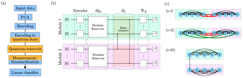
Figure 1: Schematic illustration of QERC and its architecuture. (a) QERC data flow involving classical pre-processing, a quantum reservoir, and a trainable classical linear classifier. (b) The architecture of the quantum reservoir. It consists of modular level reservoirs $\mathcal{U}_{\mathrm{M}}$, followed by inter-modular connections $\mathcal{U}_{\mathrm{c}}$, and then single qubit rotations $\mathcal{R}_{X}$ before the measurement in the computational basis. (c) Different configurations of reservoir connections featuring various inter-modular links.

II Architecture and Model

A schematic illustration of the architecture of QERC is depicted in Fig. 1, which consists of a classical pre-processor, a quantum reservoir, and a classifier using a one-layer classical neural network. To understand the effect of long-range connections within the quantum component of the system, we employ a general $m$-module structure for the quantum reservoir where the inter-module connections are explicitly separated from the intra-module connections, as illustrated in Fig. 1b, allowing a clear comparison of the long-range effects.

For the pre-processor, the PCA is used to compress the data and then the largest $2n$ PCA components are encoded into the $n$ qubits as an initial state $|\psi_{0}\rangle$ [37]. Rescaling is used to ensure the data can be sufficiently spread out over the Bloch sphere for each qubit.

Next, the state will be under the action of the quantum reservoir, which can described by an unitary of the form $\mathcal{U}=\mathcal{R}_{X}\mathcal{U}_{\mathrm{c}}\mathcal{U}_{\mathrm{M}}$. As illustrated in Fig. 1b, the quantum reservoir architecture considered here consists of three components: modular-level reservoirs $\mathcal{U}_{\mathrm{M}}$, inter-modular connections $\mathcal{U}_{\mathrm{c}}$, and single qubit operations $\mathcal{R}_{X}$ followed by measurements.

Now the modular-level reservoirs $\mathcal{U}_{\mathrm{M}}$ comprise $m$-modules, specifically denoted by the sequence $[n^{(1)},n^{(2)},\ldots,n^{(m)}]$, where each $n^{(k)}$ represents the number of qubits in the $k$-th module, so $n=\sum_{k}n^{(k)}$ is the total number of qubits in the whole system. The modular reservoir for the $k$-th module is given by the unitary $\mathcal{U}^{(k)}$ meaning the overall action on the initial state by all modular reservoirs is described by $\mathcal{U}_{\mathrm{M}}=\prod_{k}\mathcal{U}^{(k)}$. There are many choices for the modular reservoir, which is usually based on physical systems, such as various Ising models and random unitaries [37, 38]. In particular, previous studies suggests that $ZZ$ interactions followed by $X$ is sufficient to realize a high performance reservoir [37]. As such we consider the Hamiltonian

$$H^{(k)} =\hbar\sum_{i,j}J_{ij}^{(k)}Z_{i}Z_{j},$$ (1)

which gives the unitary $\mathcal{U}^{(k)}=\exp(-i\sum_{ij}\theta_{J,ij}^{(k)}Z_{i}Z_{j})$ where $\theta_{J,ij}^{(k)}=J_{ij}^{(k)}t$. The distance-dependent connections within the same module are given $\theta_{J,ij}^{(k)}=\theta_{J}/|i-j|^{\alpha},$ where $\theta_{J}$ is a control parameter of the reservior (chosen equal to $2\pi$ here [39]), while $\alpha$ is the interaction exponent. Based on physical systems, $\alpha$ may take various values ranging from $\alpha=0$ to $6$. In particular, $\alpha=1.5$ is typical in ion traps, [40, 41], $\alpha=2$ for Coulomb-type interactions, $\alpha=3$ for dipole-dipole interactions, and $\alpha=6$ for Van der Waals-type interactions [23, 42].

Second, interactions between modules are introduced via $\mathcal{U}_{c}$ following the application of the local module operations $\mathcal{U}_{\mathrm{M}}$. The inter-modular connections can take a different form from (1), but here we choose the same $ZZ$ interactions for convenience. This choice allows the use of the well-understood dynamics of $ZZ$ interactions and simplifies our analysis. The inter-modular Hamiltonian has the form

$$H_{c} =\hbar\sum_{i,j}c_{ij}Z_{i}Z_{j},$$ (2)

where the index $i$ and $j$ now belongs to different modules. The corresponding unitary operation is given by $\mathcal{U}_{c}=\exp(-i\sum_{ij}\theta_{c,ij}Z_{i}Z_{j})$ with $\theta_{c,ij}=c_{ij}t$. For simplicity, we focus on the uniform case $\theta_{c,ij}=\theta_{c}$. In particular, the interaction $Z_{i}Z_{j}$ with $\theta_{c}=\pi/4$ is an interesting regime, because it is equivalent to a controlled-$Z$ gate up to local operations, and in principle can create maximum entanglement between unentangled qubits.

Third, single qubit operations $\mathcal{R}_{X}$ precede the final measurement in the computational basis. These together determine the measurement basis. This is important because the entangling effect of additional phase added by $\mathcal{U}_{c}$ cannot be observed in the computational basis. Here, we use $\mathcal{R}_{X}=\prod_{i}R_{X,i}(\theta_{g})=\prod_{i}\exp(-i\theta_{g}X_{i})$ to change the measurement angles by using single qubit rotations before measurement. Previous results suggest that parameters around $\theta_{J}=2\pi$ and $\theta_{g}=\pi/8$ give good performance for $\alpha=1.5$ [39], which is adopted for the following results. Finally, the evolved state $\mathcal{U}|\psi_{0}\rangle$ is then measured in the computational basis, and the probability distribution is sampled. The process is repeated for all training datasets, and the probability distributions are then standardized and fed into a one-layer neural network classifier for training.

The main focus of this paper is now on how the performance of QERC on machine learning classification tasks are affected by these connections. Specifically, we measure the test accuracy $\eta$, which is the fraction of test data correctly classified into the target class, after the training process of QERC. Our performance is quantified by determining the test accuracy of the QERC system for the classification task being undertaken. In particular, the classification task considered is the MNIST digit dataset. We will now explore various types of connections within the modular structure impact this performance.

III Single chain with finite range connections

To explore the necessity and effect of long-range connections in QERC, we first examine the impact of interaction range in a single-chain system. Our results suggest that certain finite cutoff range is enough and motivate us to use module architecture. Here, we consider a single module ($m=1$) with no inter-module connections $\theta_{c}=0$. Our single module consists of a uniformly spaced chain of qubits interacting with interaction strength $\theta_{J,ij}$ defined as:

$$\theta_{J,ij}=\begin{cases}\frac{2\pi}{|i-j|^{\alpha}}&\text{for }|i-j|\leq R,\\ 0&\text{otherwise}.\end{cases}$$ (3)

where $R$ is the cutoff radius for the connections defining the maximum distance over which qubit interactions are considered. By varying $R$, it naturally allows the investigation of the effects of finite interaction ranges of connections within the chain.

Fig. 2 shows the test accuracy for image classification as a function of the interaction exponent $\alpha$ and the cutoff distance $R$ for a chain with $n=10$ qubits. Here, all-to-all connections correspond to $R=9$, which have the highest performance across a wide range of $\alpha$ values from approximately 0.1 to 2. As $R$ decreases, dependence on $\alpha$ becomes more significant. In particular, for $R\lesssim 4$, certain values of $\alpha$, such as $\alpha=1$ and $\alpha=2$, shows lower test accuracy. On the other hand, for sufficiently large interaction ranges, $R\gg 4$, the choice of $\alpha$ becomes less important. Similar cutoff radii $R$ with performance plateaus are observed for different chain lengths with n=8,12, indicating that a certain finite range of interaction may be sufficient to achieve similar QERC performance as with all-to-all coupling. This observation raises questions about the advantages of using very long-range coupling over shorter ranges. A modular system, with a focus on inter-module connections, provides a clear framework for exploring and comparing these long- and short-range interactions.

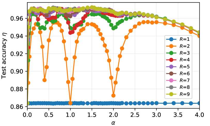
Figure 2: Test accuracy $\eta$ for the MNIST digit dataset classification task on a single 10 qubit chain configuration module vs interaction exponent $\alpha$ for varying interaction range $R$ with $\theta_{g}=\pi/8$.

IV Effect of inter module connections on the performance

(a)		$R_{\times}=0$	$R_{\times}=1$	$R_{\times}=2$	$R_{\times}=3$
	$n_{\ell}$	($n_{\times}=0$)	($n_{\times}=1$)	($n_{\times}=3$)	($n_{\times}=6$)
$\alpha=1.0$	0	0.9112	0.9269	0.9360	0.9565
	1	0.9313	0.9463	0.9506	-
	2	0.9464	0.9520	-	-
	3	0.9531	-	-	-
$\alpha=1.5$	0	0.9520	0.9514	0.9588	0.9629
	1	0.9561	0.9586	0.9636	-
	2	0.9599	0.9619	-	-
	3	0.9636	-	-	-
$\alpha=2.0$	0	0.9376	0.9404	0.9437	0.9624
	1	0.9495	0.9544	0.9549	-
	2	0.9576	0.9597	-	-
	3	0.9614	-	-	-

(b)		$R_{\times}=0$	$R_{\times}=1$	$R_{\times}=2$	$R_{\times}=3$
	$n_{\ell}$	($n_{\times}=0$)	($n_{\times}=1$)	($n_{\times}=3$)	($n_{\times}=6$)
$\alpha=1.0$	0	0.9112	0.9294	0.9382	0.9573
	1	0.9362	0.9484	0.9532	-
	2	0.948	0.958	-	-
	3	0.958	-	-	-
$\alpha=1.5$	0	0.9520	0.9538	0.9604	0.9631
	1	0.9572	0.9595	0.9641	-
	2	0.962	0.963	-	-
	3	0.964	-	-	-
$\alpha=2.0$	0	0.9376	0.9424	0.9469	0.9631
	1	0.9518	0.9545	0.958	-
	2	0.958	0.960	-	-
	3	0.961	-	-	-

Table 1: Test accuracy for the [5,5]-module structure over all possible configurations for modules with cross connection radius $R_{\times}$ and number of arbitrary connections $n_{\ell}$. For $R_{\times}=0,1,2,3$, there are number of cross connections $n_{\times}=0,1,3,6$ respectively (a) Highest test accuracy $\eta^{*}$ over all configurations with $\theta_{c}=\pi/4$ (b) Highest test accuracy $\eta^{*}$ over all configurations and $\theta_{c}$.

Let us now consider splitting our single chain into two modules ($m=2$) with inter-connections to better compare the advantages of different types of connections. The observation of $R\gg 4$ with no further substantial improvements suggests that a [5,5]-module structure should capture the key features of the system. In particular, connections near the boundary (red lines in Fig. 1c) are of interest, because they allow for direct comparison with the single chain setup with $R=4$ discussed in the ealier. With these insights, we will focus on interaction decay rates $\alpha=1$, $1.5$, and $2$, which correspond to systems with high symmetry, high performance, and typical physical interactions, respectively.

We begin by introducing the cross-interaction strength, defined as

$$\theta_{c,ij}=\begin{cases}\theta_{c}&\text{for }|i-j|\leq R_{\times},\\ 0&\text{otherwise}.\end{cases}$$ (4)

where $i$ and $j$ are the indices for the first and second modules, respectively, as indicated by the node indices in Fig. 1c-i, while $R_{\times}$ is the cutoff radius for these nodes. When $R_{\times}=4$, the connection topology matches that of $R=4$ in the previous section, except for the interaction strength. These connections are assumed to operate through mechanisms other than geometric distance, such as wired connections between nodes, so that the interaction may be controlled independently. As such it is a good initial starting point.

In addition to the $R_{\times}$, which consists of $n_{\times}$ connections, we can also have arbitrary connections that are not constrained along the boundary. The number of those remaining connections is denoted by $n_{\ell}$, illustrated as green line in Fig. 1c-ii. Since there are many configurations with a given variable, the best test accuracy $\eta^{*}(R_{\times},n_{\ell})$ over all configurations is considered below.

IV.1 Two modules with $\theta_{c}=\pi/4$

It is interesting to see whether the number of arbitrary connections $n_{\ell}$ enhances performance more effectively than connections across the boundary. First, let us focus on $\alpha=1$ as shown in Table 1a with $\theta_{c}=\pi/4$. For two completely separated modules with no inter-connections ($R_{\times}=0,n_{\ell}=0$) as shown in upper left in Table 1a, the highest test accuracy is $91.12\%$. Next we can consider adding connections near the boundary by using $R_{\times}=0,1,2,3$, corresponding to the number of connections $n_{\times}=0,1,3,6$. For just one connection at the boundary $R_{\times}=1$, the performance significantly increases by $1.6\%$ to $92.69\%$. In general, as $R_{\times}$ increases with more connections, the test accuracy increases.

For arbitrary connections, the best test accuracy increases as more connections $n_{\ell}$ are added. Notably, a single good arbitrary connection $\eta^{*}(R_{\times}=0,n_{\ell}=1)$ can perform $0.4\%$ better than the one boundary connection $\eta^{*}(R_{\times}=1,n_{\ell}=0)$. The best test accuracy for any given $n_{\ell}$ always outperforms or equals that of the same number of boundary connections by definition, as clearly shown by comparing $\eta^{*}(R_{\times}=0,n_{\ell})$ with $\eta^{*}(R_{\times}=1,n_{\ell}-1)$ in Table 1a. The more interesting result is that 2 arbitrary connections $\eta^{*}(R_{\times}=0,n_{\ell}=2)$ can outperform 3 connections near the boundary $\eta^{*}(R_{\times}=2,n_{\ell}=0)$. Moreover, 3 arbitrary connections $\eta^{*}(R_{\times}=0,n_{\ell}=3)$ can achieve a best test accuracy comparable with 6 boundary connections $\eta^{*}(R_{\times}=3,n_{\ell}=0)$. These findings hold for other values of $\alpha$ as well, suggesting that network topology plays a crucial role. Specifically, a few well-placed connections between two modules can achieve performance comparable to higher number of connections across the boundary, and therefore close with the performance of all-to-all connectivity. This indicates that modular structure actually provide a good way to explore the inter-connections and offer an alternative implementation to all-to-all connections.

IV.2 Two modules with arbitrary $\theta_{c}$

In general, $\theta_{c}=\pi/4$ is considered as a good choice as discussed above. However, due to the many connections in the Hamiltonian, certain interactions might reduce entanglement between modules. Fig. 3 shows the change in the performance as the inter-module connections $\theta_{c}$ increase. The performance increases initially as $\theta_{c}$ increases, with the highest performance happening near, but not exactly at, $\theta_{c}\approx\pi/4$ or $\theta_{c}\approx 3\pi/4$. This suggests that $\theta_{c}=\pi/4$, used in the previous subsection, is indeed a good choice. The qualitative conclusions and comparisons between arbitrary connections remain valid, as shown in Table 1b, which is the results of the best test accuracy over different configurations and $\theta_{c}$. The slightly higher best performance compared to Table 1a, indicates that $\theta_{c}=\pi/4$ is rarely the optimal best choice, but it is still a good choice. Therefore, for better performance, $\theta_{c}$ may be treated as a tunable hyper-parameter to be optimized in simulations and experiments.

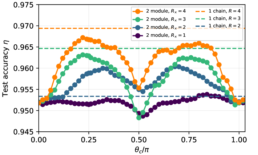
Figure 3: Test accuracy of the [5,5]-module structure with $\alpha=1.5$ for $R_{\times}=1,2,3,4$ vs inter-modular interaction strength $\theta_{c}$. The horizontal dotted lines are 1 single chain with $R$ cutoff radius for comparison.

With these results, we can further compare the single chain with two modules with inter-connections as shown in Fig. 3. The horizontal dashed lines show the corresponding test accuracy of single chain with different $R$. For the two module with $R_{\times}=3$, it has one more connection in each module compared with a single chain with $R=3$, and the performance is still slightly lower. In addition, the $R_{\times}=4$ and $R=4$ has the same connections topology but with different interaction strength for the connections across the boundary. With best $\theta_{c}$, the performance of two modules can be quite close but is still lower than the single chain, which suggests further fine tuning each $\theta_{c,ij}$ independently can achieve even higher performance.

V Parallel connections

In addition to the boundary and arbitrary connections considered in the previous section, we can also consider the one-to-one parallel connections, as illustrated by the example in Fig. 1c-iii. This configuration is more practical in two dimensions, where inter-modular connections are more difficult to cross each other. In particular, we consider the modules with equal size $n^{(1)}=n^{(2)}$, and the set of possible parallel connections are given by the dotted line in the inset of Fig. 4a. We explore all possible subsets of these parallel connections with each connection of interaction strength $\theta_{c}$. The particular configuration considered here is the [5,5]-module structures where there can have 5 parallel connections between two modules, and therefore, total $2^{5}=32$ possible configurations. The best test accuracy for the given number of parallel connections $n_{\ell}$ with $\theta_{c}=\pi/4$ are shown in Fig. 4a. It is clear that the performance increases with the number of parallel connections $n_{\ell}$. Also, the best test accuracy for over both $n_{\ell}$ and $\theta_{c}$ is plotted in the same figure, and the best test accuracy increase up to a certain point, after which additional connections yield diminishing returns. In particular, with only $n_{\ell}=4$ connections, the performance improved for more than 1% and is near the best performance for two modular systems. This result, when compared with the arbitrary connections, as plotted in Fig. 4a, indicates that the parallel connections are already a good connections topology for QERC.

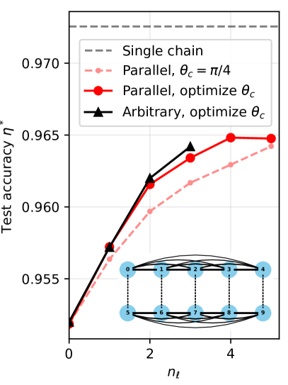
Figure 4: Highest test accuracy for $\alpha=1.5$ across all inter-modular configurations with $\theta_{c}=\pi/4$, plotted as a function of the number of connections $n_{\ell}$. (a) [5,5]-module structures with parallel configurations ($\theta_{c}=\pi/4$). The solid curves for the parallel and arbitrary also show the highest test accuracy over different $\theta_{c}$ . (b) [5,5,5]-module structures with parallel configurations among connected 2- and 3-modules. The dashed gray line indicates performance for a single chain of the same total qubit count. Insets illustrate connection structures.

The modular architecture enables a clear separation of at least two sources of performance contributions: the modular reservoirs themselves and the inter-connections between them. For the reservoirs, previous studies have suggested that random unitary reservoirs can perform comparably or even better than most physical reservoirs [38] (see Appendix A for a comparison of ZZ and random reservoirs). The optimal setup of two random modular reservoirs without inter-connections is expected to perform near optimally; however, adding just a single quantum connection can still substantially improve performance (see Appendix A). This clearly suggests that just one single quantum connection allows the improvement of the performance beyond the best of two independent modules.

VI Parallel connections in three modules

The performance improvement of the parallel connections observed in the previous section indicates that this architecture may be sufficiently good for QERC. To further explore the potential of parallel connections, we expand the architectural analysis to include three-modules. In particular, we consider $m=3$, with [5,5,5]-module structure (see inset of Fig. 4b). There are 5 connections between the first and second modules, and 5 connections between the second and third modules. Therefore, there can have maximum 10 parallel connections and $1024$ possible connection configurations. Most of the configurations have all qubits in all modules connected through the network of pairwise interactions. However, some configurations have no pariwise cross-module connections, which means that they are not entangled and can be simulated separated. These two possibility are considered as the connected modules, and disconnected modules respectively.

The results are shown in Fig. 4b for $\theta_{c}=\pi/4$, with the best test accuracy over all the configurations with the same $n_{\ell}$. For the disconnected modules, there are at most 5 connections and the maximum performance happens at $n_{\ell}=4$, which behaves similar to the result in Fig. 4a. For the connected modules, the result is close to the disconnected modules and the best test accuracy keeps increasing until $n_{\ell}=8$. At that point, the performance is very close to a single module with all-to-all distance dependence interactions. This suggests that roughly 8 connections out of 75 inter-module connections in [5,5,5]-module may be sufficient for QERC to operate in this modular architecture. In addition, the parallel connections in this modular architecture may be easier to be implemented in a 2D chip, and it suggests an alternative implementation over the all-to-all connections.

Comparison of Fig. 4 a and Fig. 4b at $\theta_{c}=0$ also show that the three independent modules together already perform better than two independent modules. This is partially contributed by the increasing of the Hilbert space dimension and the processing of more input PCA components using more qubits. It suggests that we may be able to use the multiple small quantum reservoirs, or reuse the same reservoir to process the input to achieve high performance. Nonetheless, we still need the quantum connections to get even higher performance.

VII Conclusion and discussion

In this work, we explored the role of long-range and module connections in the performance of QERC. Our results indicate that sufficient finite-range connections can achieve comparable performance to all-to-all connections. The modular architecture of quantum reservoirs allows for a better understanding of the effects and performance contribution of inter-modular connections. In particular, various connection configurations demonstrated that even a few well-placed connections can significantly enhance performance. Furthermore, introducing a single quantum connection between nearly optimal individual reservoirs can still enhance performance.

These results suggest the possibility of simplifying the implementation of reservoir computing in quantum computers. The modular structure with non-crossing connections is more compatible with the layout of two-dimensional quantum chips [43]. Similar modular structures have been considered in certain variational ansatzes to reduce entanglement and facilitate modularity in quantum circuits [44, 45, 46, 47]. In ion-based quantum computers with all-to-all two-qubit gates [48], employing a small number of connections can still reduce computational time. Alternatively, the integration of several small and simple quantum systems may be easier to implement in reservoir experiments, aligning more closely with distributed quantum computing [49]. Therefore, modular reservoirs have the potential to tackle complex machine learning tasks more effectively.

Appendix A: CUE modular reservoirs

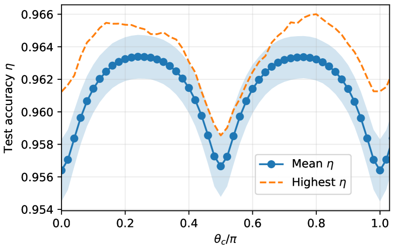
Structure	Best performance	Improvement %
[1,1]	47.2%	+6.9%(54.1%)
[2,2]	76.7%	+3.4%(80.1%)
[5,5]	96.3%	+0.7%(95.6%)

Figure 5: Test accuracy versus $\theta_{c}$ for the random unitary with one link. The blue solid line represents the mean performance over the samples from CUE. The shaded area indicates the standard deviation. The dotted line shows the performance of the best local CUE module with the addition of a single link and [5,5]-module structures. (table) Best test accuracy of the QERC with two random modular reservoirs after adding one additional connection, optimal values over all possible $\theta_{c}$.

To evaluate the typicality of the performance improvement, we can compare it with the performance of randomly sampled unitary reservoirs for each module. In particular, we consider 300 random unitary $\mathcal{U}^{(1)}$ and $\mathcal{U}^{(2)}$, that are sampled uniformly from the Circular Unitary Ensemble (CUE). Then, one inter-modular connection is added and the interaction strength $\theta_{c}$ is turned on to see how it behaves. Fig. 5 shows the mean performance versus $\theta_{c}$ for the random unitary with one link. For the modules with no inter-connections ($\theta_{c}=0$), the mean performance is $95.6\%$ which increases by $0.76\%$ on average when the interaction $\theta_{c}$ is turned on. For the best modular random unitary reservoirs, the performance improvement is about $0.4\%$. These results are comparable with $0.5\%$ improvement for $ZZ$ reservoir in Fig. 4a with $n_{\ell}=1$. The mean performance of random reservoirs with 1 connections is also comparable with 2 connections for the $ZZ$ reservoirs.

In addition, even for the separable reservoirs with the best performed realization $\mathcal{U}^{(1)}$ and $\mathcal{U}^{(2)}$, one additional connection with $\theta_{c}$ turned on can still have performance improvement. This improvement of the addition of the connections for the near-optimal reservoir is true for other modular sizes as shown in the table. These results suggest clearly that just one single quantum connection allows the improvement of the performance beyond the best of two independent modules.

References

- Biamonte et al. [2017] J. Biamonte, P. Wittek, N. Pancotti, P. Rebentrost, N. Wiebe, and S. Lloyd, Quantum machine learning, Nature 549, 195 (2017).
- Cerezo et al. [2022] M. Cerezo, G. Verdon, H.-Y. Huang, L. Cincio, and P. J. Coles, Challenges and opportunities in quantum machine learning, Nat Comput Sci 2, 567 (2022).
- Huang et al. [2021] H.-Y. Huang, M. Broughton, M. Mohseni, R. Babbush, S. Boixo, H. Neven, and J. R. McClean, Power of data in quantum machine learning, Nat Commun 12, 2631 (2021).
- Schuld and Killoran [2019] M. Schuld and N. Killoran, Quantum Machine Learning in Feature Hilbert Spaces, Phys. Rev. Lett. 122, 040504 (2019).
- Ristè et al. [2017] D. Ristè, M. P. da Silva, C. A. Ryan, A. W. Cross, A. D. Córcoles, J. A. Smolin, J. M. Gambetta, J. M. Chow, and B. R. Johnson, Demonstration of quantum advantage in machine learning, npj Quantum Inf 3, 1 (2017).
- Tang [2022] E. Tang, Dequantizing algorithms to understand quantum advantage in machine learning, Nat Rev Phys 4, 692 (2022).
- Cerezo et al. [2021a] M. Cerezo, A. Arrasmith, R. Babbush, S. C. Benjamin, S. Endo, K. Fujii, J. R. McClean, K. Mitarai, X. Yuan, L. Cincio, and P. J. Coles, Variational quantum algorithms, Nat Rev Phys 3, 625 (2021a).
- Anschuetz and Kiani [2022] E. R. Anschuetz and B. T. Kiani, Quantum variational algorithms are swamped with traps, Nat Commun 13, 7760 (2022).
- Skolik et al. [2022] A. Skolik, S. Jerbi, and V. Dunjko, Quantum agents in the Gym: a variational quantum algorithm for deep Q-learning, Quantum 6, 720 (2022).
- Farhi et al. [2014] E. Farhi, J. Goldstone, and S. Gutmann, A Quantum Approximate Optimization Algorithm, arXiv:1411.4028 (2014).
- Tilly et al. [2022] J. Tilly, H. Chen, S. Cao, D. Picozzi, K. Setia, Y. Li, E. Grant, L. Wossnig, I. Rungger, G. H. Booth, and J. Tennyson, The Variational Quantum Eigensolver: A review of methods and best practices, Physics Reports 986, 1 (2022).
- McClean et al. [2018] J. R. McClean, S. Boixo, V. N. Smelyanskiy, R. Babbush, and H. Neven, Barren plateaus in quantum neural network training landscapes, Nat Commun 9, 4812 (2018).
- Bittel and Kliesch [2021] L. Bittel and M. Kliesch, Training Variational Quantum Algorithms Is NP-Hard, Phys. Rev. Lett. 127, 120502 (2021).
- Larocca et al. [2022] M. Larocca, P. Czarnik, K. Sharma, G. Muraleedharan, P. J. Coles, and M. Cerezo, Diagnosing Barren Plateaus with Tools from Quantum Optimal Control, Quantum 6, 824 (2022).
- Cerezo et al. [2021b] M. Cerezo, A. Sone, T. Volkoff, L. Cincio, and P. J. Coles, Cost function dependent barren plateaus in shallow parametrized quantum circuits, Nat Commun 12, 1791 (2021b).
- Havlíček et al. [2019] V. Havlíček, A. D. Córcoles, K. Temme, A. W. Harrow, A. Kandala, J. M. Chow, and J. M. Gambetta, Supervised learning with quantum-enhanced feature spaces, Nature 567, 209 (2019).
- Fujii and Nakajima [2017] K. Fujii and K. Nakajima, Harnessing Disordered-Ensemble Quantum Dynamics for Machine Learning, Phys. Rev. Appl. 8, 024030 (2017).
- Mujal et al. [2021] P. Mujal, R. Martínez-Peña, J. Nokkala, J. García-Beni, G. L. Giorgi, M. C. Soriano, and R. Zambrini, Opportunities in Quantum Reservoir Computing and Extreme Learning Machines, Advanced Quantum Technologies 4, 2100027 (2021).
- Fujii and Nakajima [2021] K. Fujii and K. Nakajima, Quantum Reservoir Computing: A Reservoir Approach Toward Quantum Machine Learning on Near-Term Quantum Devices, in Reservoir Computing: Theory, Physical Implementations, and Applications (Springer, 2021) pp. 423–450.
- Götting et al. [2023] N. Götting, F. Lohof, and C. Gies, Exploring quantumness in quantum reservoir computing, Phys. Rev. A 108, 052427 (2023).
- Ghosh et al. [2019] S. Ghosh, A. Opala, M. Matuszewski, T. Paterek, and T. C. H. Liew, Quantum reservoir processing, npj Quantum Information 5, 1 (2019).
- Martínez-Peña et al. [2021] R. Martínez-Peña, G. L. Giorgi, J. Nokkala, M. C. Soriano, and R. Zambrini, Dynamical Phase Transitions in Quantum Reservoir Computing, Phys. Rev. Lett. 127, 100502 (2021).
- Bravo et al. [2022] R. A. Bravo, K. Najafi, X. Gao, and S. F. Yelin, Quantum Reservoir Computing Using Arrays of Rydberg Atoms, PRX Quantum 3, 030325 (2022).
- Xia et al. [2023] W. Xia, J. Zou, X. Qiu, F. Chen, B. Zhu, C. Li, D.-L. Deng, and X. Li, Configured quantum reservoir computing for multi-task machine learning, Science Bulletin 68, 2321 (2023).
- Govia et al. [2022] L. C. G. Govia, G. J. Ribeill, G. E. Rowlands, and T. A. Ohki, Nonlinear input transformations are ubiquitous in quantum reservoir computing, Neuromorph. Comput. Eng. 2, 014008 (2022).
- Govia et al. [2021] L. C. G. Govia, G. J. Ribeill, G. E. Rowlands, H. K. Krovi, and T. A. Ohki, Quantum reservoir computing with a single nonlinear oscillator, Phys. Rev. Res. 3, 013077 (2021).
- Kora et al. [2024] Y. Kora, H. Zadeh-Haghighi, T. C. Stewart, K. Heshami, and C. Simon, Frequency- and dissipation-dependent entanglement advantage in spin-network quantum reservoir computing, Phys. Rev. A 110, 042416 (2024).
- Dudas et al. [2023] J. Dudas, B. Carles, E. Plouet, F. A. Mizrahi, J. Grollier, and D. Marković, Quantum reservoir computing implementation on coherently coupled quantum oscillators, npj Quantum Inf 9, 1 (2023).
- Yasuda et al. [2023] T. Yasuda, Y. Suzuki, T. Kubota, K. Nakajima, Q. Gao, W. Zhang, S. Shimono, H. I. Nurdin, and N. Yamamoto, Quantum reservoir computing with repeated measurements on superconducting devices, arXiv:2310.06706 (2023).
- Kornjača et al. [2024] M. Kornjača, H.-Y. Hu, C. Zhao, J. Wurtz, P. Weinberg, M. Hamdan, A. Zhdanov, S. H. Cantu, H. Zhou, R. A. Bravo, K. Bagnall, J. I. Basham, J. Campo, A. Choukri, R. DeAngelo, P. Frederick, D. Haines, J. Hammett, N. Hsu, M.-G. Hu, F. Huber, P. N. Jepsen, N. Jia, T. Karolyshyn, M. Kwon, J. Long, J. Lopatin, A. Lukin, T. Macrì, O. Marković, L. A. Martínez-Martínez, X. Meng, E. Ostroumov, D. Paquette, J. Robinson, P. S. Rodriguez, A. Singh, N. Sinha, H. Thoreen, N. Wan, D. Waxman-Lenz, T. Wong, K.-H. Wu, P. L. S. Lopes, Y. Boger, N. Gemelke, T. Kitagawa, A. Keesling, X. Gao, A. Bylinskii, S. F. Yelin, F. Liu, and S.-T. Wang, Large-scale quantum reservoir learning with an analog quantum computer, arXiv:2407.02553 (2024).
- Innocenti et al. [2023] L. Innocenti, S. Lorenzo, I. Palmisano, A. Ferraro, M. Paternostro, and G. M. Palma, Potential and limitations of quantum extreme learning machines, Commun Phys 6, 1 (2023).
- Xiong et al. [2024] W. Xiong, G. Facelli, M. Sahebi, O. Agnel, T. Chotibut, S. Thanasilp, and Z. Holmes, On fundamental aspects of quantum extreme learning machines, arXiv:2312.15124 (2024).
- Chen et al. [2020] J. Chen, H. I. Nurdin, and N. Yamamoto, Temporal Information Processing on Noisy Quantum Computers, Phys. Rev. Appl. 14, 024065 (2020).
- Bharti et al. [2022] K. Bharti, A. Cervera-Lierta, T. H. Kyaw, T. Haug, S. Alperin-Lea, A. Anand, M. Degroote, H. Heimonen, J. S. Kottmann, T. Menke, W.-K. Mok, S. Sim, L.-C. Kwek, and A. Aspuru-Guzik, Noisy intermediate-scale quantum (NISQ) algorithms, Rev. Mod. Phys. 94, 015004 (2022).
- Fry et al. [2023] D. Fry, A. Deshmukh, S. Y.-C. Chen, V. Rastunkov, and V. Markov, Optimizing quantum noise-induced reservoir computing for nonlinear and chaotic time series prediction, Sci Rep 13, 19326 (2023).
- Domingo et al. [2023] L. Domingo, G. Carlo, and F. Borondo, Taking advantage of noise in quantum reservoir computing, Sci Rep 13, 8790 (2023).
- Sakurai et al. [2022] A. Sakurai, M. P. Estarellas, W. J. Munro, and K. Nemoto, Quantum Extreme Reservoir Computation Utilizing Scale-Free Networks, Phys. Rev. Applied 17, 064044 (2022).
- Hayashi et al. [2023] A. Hayashi, A. Sakurai, S. Nishio, W. J. Munro, and K. Nemoto, Impact of the form of weighted networks on the quantum extreme reservoir computation, Phys. Rev. A 108, 042609 (2023).
- Sakurai et al. [2024] A. Sakurai, A. Hayashi, W. J. Munro, and K. Nemoto, Simple Hamiltonian dynamics is a powerful quantum processing resource, arXiv:2405.14245 (2024).
- Porras and Cirac [2004] D. Porras and J. I. Cirac, Effective Quantum Spin Systems with Trapped Ions, Phys. Rev. Lett. 92, 207901 (2004).
- Britton et al. [2012] J. W. Britton, B. C. Sawyer, A. C. Keith, C.-C. J. Wang, J. K. Freericks, H. Uys, M. J. Biercuk, and J. J. Bollinger, Engineered two-dimensional Ising interactions in a trapped-ion quantum simulator with hundreds of spins, Nature 484, 489 (2012).
- Defenu et al. [2023] N. Defenu, T. Donner, T. Macrì, G. Pagano, S. Ruffo, and A. Trombettoni, Long-range interacting quantum systems, Rev. Mod. Phys. 95, 035002 (2023).
- [43] Ibm quantum, ibm research blog (10 may 2022).
- Eddins et al. [2022] A. Eddins, M. Motta, T. P. Gujarati, S. Bravyi, A. Mezzacapo, C. Hadfield, and S. Sheldon, Doubling the Size of Quantum Simulators by Entanglement Forging, PRX Quantum 3, 010309 (2022).
- Peng et al. [2020] T. Peng, A. W. Harrow, M. Ozols, and X. Wu, Simulating Large Quantum Circuits on a Small Quantum Computer, Phys. Rev. Lett. 125, 150504 (2020).
- Fujii et al. [2022] K. Fujii, K. Mizuta, H. Ueda, K. Mitarai, W. Mizukami, and Y. O. Nakagawa, Deep Variational Quantum Eigensolver: A Divide-And-Conquer Method for Solving a Larger Problem with Smaller Size Quantum Computers, PRX Quantum 3, 010346 (2022).
- DiAdamo et al. [2021] S. DiAdamo, M. Ghibaudi, and J. Cruise, Distributed Quantum Computing and Network Control for Accelerated VQE, IEEE Transactions on Quantum Engineering 2, 1 (2021).
- DeCross et al. [2024] M. DeCross, R. Haghshenas, M. Liu, E. Rinaldi, J. Gray, Y. Alexeev, C. H. Baldwin, J. P. Bartolotta, M. Bohn, E. Chertkov, J. Cline, J. Colina, D. DelVento, J. M. Dreiling, C. Foltz, J. P. Gaebler, T. M. Gatterman, C. N. Gilbreth, J. Giles, D. Gresh, A. Hall, A. Hankin, A. Hansen, N. Hewitt, I. Hoffman, C. Holliman, R. B. Hutson, T. Jacobs, J. Johansen, P. J. Lee, E. Lehman, D. Lucchetti, D. Lykov, I. S. Madjarov, B. Mathewson, K. Mayer, M. Mills, P. Niroula, J. M. Pino, C. Roman, M. Schecter, P. E. Siegfried, B. G. Tiemann, C. Volin, J. Walker, R. Shaydulin, M. Pistoia, S. A. Moses, D. Hayes, B. Neyenhuis, R. P. Stutz, and M. Foss-Feig, The computational power of random quantum circuits in arbitrary geometries, arXiv:2406.02501 (2024).
- Barral et al. [2024] D. Barral, F. J. Cardama, G. Díaz, D. Faílde, I. F. Llovo, M. M. Juane, J. Vázquez-Pérez, J. Villasuso, C. Piñeiro, N. Costas, J. C. Pichel, T. F. Pena, and A. Gómez, Review of Distributed Quantum Computing. From single QPU to High Performance Quantum Computing, arXiv:2404.01265 (2024).