Exploring $Z^{\prime}$ and Right-Handed Neutrinos in the BLSM at the Large Hadron Collider

Abstract

We investigate the phenomenological implications of the $B-L$ extension of the Standard Model (BLSM) at the Large Hadron Collider (LHC), with an emphasis on the production and decay of the $Z^{\prime}$ boson into pairs of right-handed neutrinos (RHNs). These decays result in three distinct channels with observable final states: (i) four leptons, (ii) three leptons plus two jets, both accompanied by missing transverse energy, and (iii) two leptons with multiple jets. To enhance sensitivity to $Z^{\prime}$ and RHN signals over the standard model background, we employ XGBOOST based analyses to optimize the selection criteria. Our findings demonstrate that these channels provide promising opportunities to probe new physics, offering critical insights into the mechanisms of neutrino mass generation and baryon asymmetry in the universe.

1 Introduction

The Standard Model (SM) of particle physics has been highly successful in explaining a wide range of phenomena, but it falls short in addressing certain critical issues. Notably, it cannot explain neutrino oscillations, which indicate that neutrinos have mass Ref. Fukuda:1998mi ; Ahn:2002up ; Eguchi:2002dm ; Ahmad:2002jz ; An:2012eh , nor the observed baryon asymmetry in the universe, where matter significantly outweighs antimatter. These deficiencies suggest that an extension of the SM is required to account for these phenomena.

One promising extension involves the introduction of right-handed neutrinos (RHN), which can naturally explain the small but non-zero masses of neutrinos through the seesaw mechanism. Additionally, extending the gauge symmetry of the SM provides a framework to incorporate new physics without fundamentally altering its successful aspects. Specifically, the $B-L$ (baryon minus lepton number) extension of the SM (BLSM) Ref. Mohapatra:1980qe ; Papaefstathiou:2011rc ; Masiero:1982fi ; Mohapatra:1982xz ; Buchmuller:1991ce ; Khalil:2006yi offers a minimal and elegant approach to address these shortcomings.

The minimal low-energy extension is achieved by augmenting the SM gauge group with an additional $U(1)_{B-L}$ symmetry, leading to the gauge group Khalil:2006yi :

$$G_{B-L}=SU(3)_{C}\times SU(2)_{L}\times U(1)_{Y}\times U(1)_{B-L}.$$ (1)

This extension, BLSM, introduces new particles and interactions that contribute to the SM phenomenology, particularly in the neutrino and baryon sectors.

1. Right-handed Neutrinos: The model introduces three RHN $\nu^{i}_{R}$ (where $i=1,2,3$), each with a $B-L$ charge of $-1$. These particles do not interact with the SM weak forces but are crucial for generating neutrino masses via the seesaw mechanism.

2. New Gauge Boson $Z^{\prime}$: The extension includes an extra gauge boson, denoted as $Z^{\prime}$, corresponding to the $B-L$ gauge symmetry. This new force carrier could have observable signatures at high-energy colliders such as the LHC, providing a direct test of the extended model.

3. Additional Scalar Field $\chi$: A new scalar field $\chi$, which is a singlet under the SM gauge group but carries a $B-L$ charge of $+2$, is introduced. This scalar plays a crucial role in breaking the $U(1)_{B-L}$ symmetry, analogous to how the Higgs field breaks the electroweak symmetry in the SM.

In this paper, we investigate the experimental signatures of these new particles, particularly the RHN and the $Z^{\prime}$ boson, at the Large Hadron Collider (LHC). The $Z^{\prime}$ boson, for instance, can manifest as a resonance in dilepton or dijet final states, serving as a potential smoking gun for physics beyond the SM. Similarly, RHNs open up novel decay channels and distinct collider signatures, offering valuable insights into the origin of neutrino masses and the baryon asymmetry of the universe. We emphasize that these signatures not only probe the existence of these particles but also serve as critical tests of the BLSM, which seeks to address several fundamental questions in particle physics. Specifically, we examine four distinct signals arising from $Z^{\prime}$ production at the LHC, where the $Z^{\prime}$ decays into two RHNs, ($\nu_{R}$). These decay channels lead to the following final states:

1. Four leptons and missing energy.

2. Three leptons, two jets, and missing energy.

3. Two leptons, and multiple jets.

4. One lepton, two jets, and missing energy.

The first three channels arise from the decay of two $\nu_{R}$ into $W$ boson and lepton, with the $W$ boson subsequently decaying either into lepton and $\nu_{L}$ or into quarks. The fourth channel occurs when one RHN decays into a $W$ boson and a lepton, with the $W$ decaying into a jet, while the second RHN decays into a $Z$ boson and $\nu_{L}$, and the $Z$ decays into two $\nu_{L}$.

The decay width of the RHN to $Z$ and $\nu_{L}$ is significantly smaller than its decay to $W$ and a lepton, resulting in a much lower cross section for the fourth channel compared to the other channels. Additionally, this channel is affected by considerable Standard Model background. Consequently, our analysis in the subsequent sections will focus exclusively on the first three channels. For the analyses, we apply XGBOOST techniques Ref. xgboost ; Xia:2018cfz ; XIA201915 ; quinlan1986induction ; quinlan1987simplifying to optimize the selection criteria and enhance the sensitivity to the $Z^{\prime}$ and RHN signatures, ensuring a clear distinction between potential new physics signals and SM background processes.

The structure of the paper is as follows: In Section 2, we provide a concise review of the BLSM, focusing on the $Z^{\prime}$ boson and RHN ($\nu_{R}$). We discuss how their masses emerge from the spontaneous breaking of the $B-L$ symmetry and outline the key interactions relevant to our analysis. This section lays the theoretical groundwork for the collider signatures examined in the subsequent sections. Section 3 is dedicated to explaining the computational methods and detailing the XGBOOST framework employed to separate signal from background. In Section 4, we analyze the above mentioned three distinct signals arising from $Z^{\prime}$ production at the LHC. Finally, Section 5 provides our conclusions and prospective remarks.

2 $Z^{\prime}$ and $\nu_{R}$ in the BLSM

As discussed above, the minimal BLSM is based on the gauge group $SU(3)_{C}\times SU(2)_{L}\times U(1)_{Y}\times U(1)_{B-L}$. The Lagrangian for this $B-L$ extension is expressed as follows:

$${\cal L}_{B-L} = i{\bar{l}}D_{\mu}\gamma^{\mu}l+i{\bar{e}_{R}}D_{\mu}\gamma^{\mu}e_{R}+i{\bar{\nu}_{R}}D_{\mu}\gamma^{\mu}\nu_{R}+i{\bar{Q}}D_{\mu}\gamma^{\mu}Q+i{\bar{d}_{R}}D_{\mu}\gamma^{\mu}d_{R}+i{\bar{u}_{R}}D_{\mu}\gamma^{\mu}u_{R}$$ (2)

$$- \frac{1}{4}W_{\mu\nu}W^{\mu\nu}-\frac{1}{4}B_{\mu\nu}B^{\mu\nu}-\frac{1}{4}C_{\mu\nu}C^{\mu\nu}+(D^{\mu}\phi)^{\dagger}(D_{\mu}\phi)+(D^{\mu}\chi)^{\dagger}(D_{\mu}\chi)$$

$$- m^{2}_{1}\phi^{\dagger}\phi-m^{2}_{2}-\lambda_{1}(\phi^{\dagger}\phi)^{2}-\lambda_{2}(\chi^{\dagger}\chi)^{2}-\lambda_{3}(\phi^{\dagger}\phi)(\chi^{\dagger}\chi)-\lambda_{e}{\bar{l}}\phi e_{R}-\lambda_{\nu}{\bar{l}}{\tilde{\phi}}\nu_{R}$$

$$- \frac{1}{2}\lambda_{\nu_{R}}{\bar{\nu}}^{c}_{R}\chi\nu_{R}-h.c.-\lambda_{d}{\bar{Q}}\phi d_{R}-\lambda_{u}{\bar{Q}}{\tilde{\phi}}u_{R}-h.c.,$$

where $C_{\mu\nu}=\partial_{\mu}C_{\nu}-\partial_{\nu}C_{\mu}$ represents the field strength tensor of the $U(1)_{B-L}$ gauge field. The covariant derivative $D_{\mu}$ is given by:

$$D_{\mu}=\partial_{\mu}-ig_{2}A^{a}_{\mu}T^{a}-Yg^{\prime}B_{\mu}-g^{{}^{\prime\prime}}Y_{B-L}C_{\mu},~~~T^{a}=\frac{\sigma^{a}}{2},~{\rm and}~\sigma^{a}{\rm are~Pauli~matrices}.$$ (3)

Here, $g^{\prime\prime}$ is the coupling constant of the $U(1)_{B-L}$ gauge group, and $Y_{B-L}$ denotes the $B-L$ quantum numbers of the particles involved, which are listed in Table 1.

	$l$	$\nu_{R}$	$e_{R}$	$Q$	$u_{R}$	$d_{R}$	$\phi$	$\chi$
$SU(2)_{L}\times U(1)_{Y}$	$({\bf 2},-1/2)$	$({\bf 1},0)$	$({\bf 1},-1)$	$({\bf 2},1/6)$	$({\bf 1},2/3)$	$({\bf 1},-1/3)$	$({\bf 2},1/2)$	$({\bf 1},0)$
$U(1)_{B-L}$	$-1$	$-1$	$-1$	$1/3$	$1/3$	$1/3$	0	2

Table 1: The $SU(2)_{L}\times U(1)_{Y}$ and $U(1)_{B-L}$ quantum numbers of the particles in the model.

To analyze the breaking of $B-L$ and electroweak symmetries, we consider the most general Higgs potential that remains invariant under these symmetries. The potential is expressed as:

$$V(\phi,\chi)=m_{1}^{2}\phi^{\dagger}\phi+m_{2}^{2}\chi^{\dagger}\chi+\lambda_{1}(\phi^{\dagger}\phi)^{2}+\lambda_{2}(\chi^{\dagger}\chi)^{2}+\lambda_{3}(\chi^{\dagger}\chi)(\phi^{\dagger}\phi),$$ (4)

where $\lambda_{3}>-2\sqrt{\lambda_{1}\lambda_{2}}$ and $\lambda_{1},\lambda_{2}\geq 0$ to ensure that the potential is bounded from below. These conditions represent the stability requirements of the potential. Furthermore, to prevent $\langle\phi\rangle=\langle\chi\rangle=0$ from being a local minimum, we assume that $\lambda_{3}^{2}<4\lambda_{1}\lambda_{2}$. Similar to the usual Higgs mechanism in the SM, the vacuum expectation values (vevs) $v$ and $v^{\prime}$ can only emerge if the squared mass terms are negative, i.e., $m_{1}^{2}<0$ and $m_{2}^{2}<0$.

After the breaking of $B-L$ gauge symmetry, the gauge field $C_{\mu}$, referred to as $Z^{\prime}$ in the remainder of this paper, acquires the following mass:

$$M_{Z^{\prime}}^{2}=4g^{\prime\prime 2}v^{\prime 2}.$$ (5)

The experimental searches at high energies place lower bounds on the mass of this extra neutral gauge boson. The most stringent constraint comes from the LEP II experiment Carena:2004xs . As an $e^{+}e^{-}$ collider, LEP II was highly effective in constraining additional gauge bosons that significantly couple to electrons. Moreover, recent results from the CDF II experiment CDF:2006krg are consistent with the LEP II constraints on the $Z^{\prime}$ mass in the context of the $B-L$ extension of the SM. Based on these findings, the typical lower bound on $M_{Z^{\prime}}$ is:

$$\frac{M_{Z^{\prime}}}{g^{\prime\prime}}>7~\text{TeV}.$$ (6)

From Eq. (5), this implies that $v^{\prime}\gtrsim\mathcal{O}(\text{TeV})$.

In addition, after the $U(1)_{B-L}$ symmetry breaking Khalil:2006yi , the Yukawa interaction term $\lambda_{\nu_{R}}\chi\bar{\nu}^{c}_{R}\nu_{R}$ generates a mass for the right-handed neutrino, given by:

$$M_{R}=\frac{1}{2\sqrt{2}}\lambda_{\nu_{R}}v^{\prime}.$$ (7)

Moreover, electroweak symmetry breaking results in the Dirac neutrino mass term:

$$m_{D}=\frac{1}{\sqrt{2}}\lambda_{\nu}v.$$ (8)

Thus, the mass matrix for the left- and right-handed neutrinos is:

$$\left(\begin{array}[]{cc}0&m_{D}\\ m_{D}&M_{R}\\ \end{array}\right).$$ (9)

Since $M_{R}$ is proportional to $v^{\prime}$ and $m_{D}$ is proportional to $v$, it follows that $M_{R}>m_{D}$. Diagonalizing this mass matrix yields the following masses for the light and heavy neutrinos, respectively:

$$m_{\nu_{L}}=-m_{D}M_{R}^{-1}m_{D}^{T},$$ (10)

$$m_{\nu_{H}}=M_{R}.$$ (11)

Thus, the $B-L$ gauge symmetry provides a natural framework for the seesaw mechanism. However, the scale of $B-L$ symmetry breaking, $v^{\prime}$, remains arbitrary. As in Ref. Khalil:2006yi , $v^{\prime}$ is assumed to be of order TeV, making $M_{R}$ also of that scale.

The $Z^{\prime}$ boson can be produced in hadron colliders, such as the LHC, through its couplings to quarks. While it can decay into various final states Ref. atlas2019zprime ; leike1999zprime ; langacker2009zprime , we focus on the scenario where the $Z^{\prime}$ decays into a pair of right-handed neutrinos. This scenario is particularly interesting because the subsequent decay of the neutrinos into a lepton and a $W$ boson can lead to a final state with two same-sign leptons, when the $W$ boson decays into jets. Such a final state is extremely rare in the SM, making it a cleaner and more distinctive probe for the $Z^{\prime}$.

The cross-section for the process $pp\to Z^{\prime}\to\nu_{R}\nu_{R}$ can be expressed as:

$$\sigma(pp\to Z^{\prime}\to\nu_{R}\nu_{R})=\int dx_{1}dx_{2}\,f_{q}(x_{1},Q^{2})f_{\bar{q}}(x_{2},Q^{2})\,\hat{\sigma}(\hat{s}),$$ (12)

where $f_{q}(x_{1},Q^{2})$ and $f_{\bar{q}}(x_{2},Q^{2})$ are the parton distribution functions (PDFs) for the quark and antiquark inside the protons Ref. cteq1995pdfs ; nnpdf2015pdfs , evaluated at momentum fractions $x_{1}$ and $x_{2}$, and scale $Q^{2}$. The $\hat{\sigma}(\hat{s})$ is the partonic cross-section for $q\bar{q}\to Z^{\prime}\to\nu_{R}\nu_{R}$, with $\hat{s}=x_{1}x_{2}s$ is the partonic center-of-mass energy squared, where $s$ is the total hadronic center-of-mass energy squared. The partonic cross-section is given by:

$$\hat{\sigma}(\hat{s})=\frac{4\pi^{2}}{\hat{s}}\frac{\Gamma(Z^{\prime}\to q\bar{q})\Gamma(Z^{\prime}\to\nu_{R}\nu_{R})}{(M_{Z^{\prime}}^{2}-\hat{s})^{2}+M_{Z^{\prime}}^{2}\Gamma_{Z^{\prime}}^{2}},$$ (13)

where$M_{Z^{\prime}}$ and $\Gamma_{Z^{\prime}}$ are the mass and total decay width of the $Z^{\prime}$ boson. The partial decay widths of the $Z^{\prime}$ boson $\Gamma(Z^{\prime}\to q\bar{q})$ and $\Gamma(Z^{\prime}\to\nu_{R}\nu_{R})$ are given by

$$\Gamma(Z^{\prime}\to q\bar{q}) = \frac{n_{q}}{216\pi}g_{B-L}^{2}M_{Z^{\prime}},$$ (14)

$$\Gamma(Z^{\prime}\to\nu_{R}\nu_{R}) = \frac{n_{\nu_{R}}}{24\pi}g_{B-L}^{2}M_{Z^{\prime}}.$$ (15)

where $n_{q}=6$, representing the six active quark flavors, as the $Z^{\prime}$ mass is generally greater than twice the top quark mass, and $n_{\nu_{R}}=3$.

3 The BLSM benchmark signatures and the computational setup

We are interested in studying the production of the $Z^{\prime}$ boson at the LHC, and its subsequent decay to right-handed neutrinos ($\nu_{R}$), which then decay to a lepton and a $W$ boson

$$pp\rightarrow Z^{\prime}\rightarrow\nu_{R}\nu_{R},~~\nu_{R}\rightarrow lW.$$

. The various combinations of the leptonic and hadronic decay channels of the $W$ boson leads to three different signatures at the colliders:

1. FS1: $2l+4$ jets

2. FS2: $3l+2$ jets $+$ MET

3. FS3: $4l+$ MET

In our analysis, we consider electrons and muons as leptons and light jets (from the hadronisation of $u,d,s,c$ quarks). We include the $\tau$ leptons in the generation, which can decay to electrons or muons. The missing transverse energy (MET, $p_{T}^{\rm miss}$) comes from the neutrinos, which are invisible in the detector leading to a momentum imbalance in the transverse plane of the collision. Fig. 1 shows the Feynman diagrams of the processes leading to the three final states discussed above.

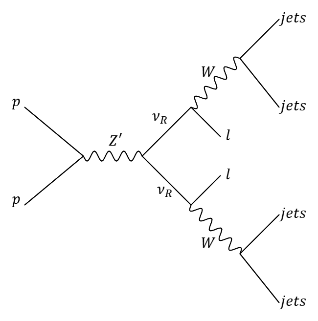
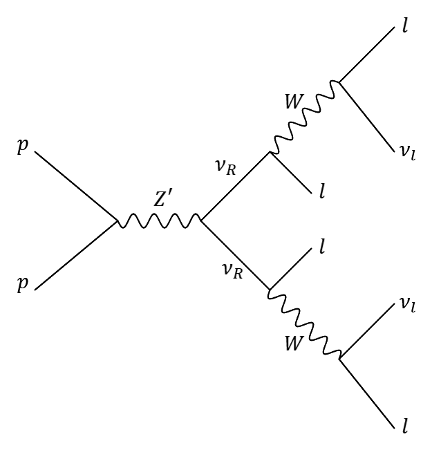
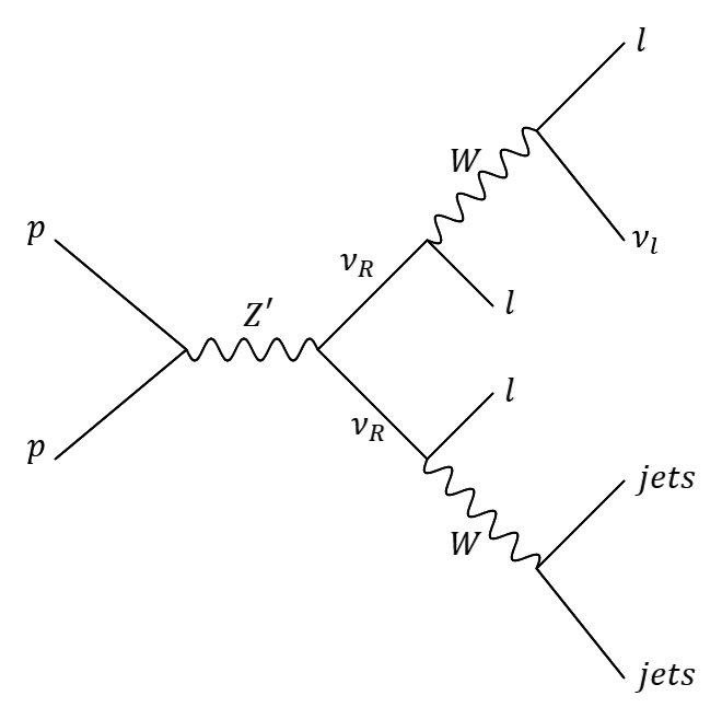
Figure 1: Feynman diagrams of the processes that we explore in this study.

In the first final state, where both the $W$ boson decay hadronically, we can have two same sign leptons along with four jets. This is a much cleaner signal since the SM background for events with two same-sign leptons is negligible. However, a contribution from the charge misidentification of leptons can lead to same-sign lepton pair even from SM backgrounds as been reported by the ATLAS/CMS collaborations CMS:2015xaf ; CMS:2018rym ; ATLAS:2019jvq . In the next two final states, the $W$ boson has a semi-leptonic and fully leptonic decay, respectively. Therefore, we don’t have same-sign leptons and the final states are characterised by MET from the neutrinos. The SM backgrounds leading to the above final states are $-$ $t\bar{t}$(dileptonic) $+2j$, $WZ$(leptonic) $+2j$, $VVV$, $V\equiv W/Z$. In addition to this, we also generate an inclusive background of $pp\rightarrow 2l4j$ for the first final state.

We now discuss the computational setup used in this study. We use the BLSM model implemented in SARAH-4.15.1 staub2014sarah to generate the Feynman rules for the model and then use SPheno-4.0.5 porod2003spheno to generate the BLSM particle spectra for different input parameters at low scale. We find a benchmark which satisfies the present constraints from LHC searches of $Z^{\prime}$, $\nu_{R}$, extra Higgs boson, and properties of the discovered 125 GeV Higgs boson. We tabulate the parameters of our benchmark point in Table 2.

$M_{Z^{\prime}}$	$M_{\nu_{R,1}}$	$g^{\prime\prime}(g_{B-L})$	$g_{YB}$
3 TeV	420 GeV	0.42	-0.55

Table 2: Details of our benchmark point in BLSM.

To study the sensitivity of this benchmark at the LHC, we simulate these processes in proton proton collisions at a centre-of-mass energy of 14 TeV. We generate events for the signal and background processes using MadGraph5_aMC (MG5), Ref. alwall2014madgraph5 where for the signal we use the BLSM UFO file generated using the SARAH framework. We use the fast detector simulation Delphes-3.5 Ref. deFavereau2014delphes for adding the detector effects and reconstructing detector-level objects, like the leptons, jets and MET, which constitute our final state.

In classification problems, like the one we study here to classify the BLSM signal events from the SM backgrounds, the conventional analyses make use of cuts placed on the distributions of various kinematic variables which have different shapes for the signal and the backgrounds. But in many cases, it is complicated to identify the most powerful variable to discriminate the signal from the background. Moreover, the cut-based analyses won’t be sensitive to situations where the boundary between the signal and the background events in multi-variable phase space is not rectangular. Therefore, in cases where no single variable is powerful enough to discriminate between the signal and the background, however, the correlations of multiple variables do have some differences, employing a more sophisticated algorithm is recommended. For analysing the three signatures at the LHC, we train a machine learning model based on the XGBOOST algorithm (eXtreme Gradient Boosting) xgboost .

In the XGBOOST algorithm, unlike the cut-based analysis, events rejected by a particular cut on some variable is not rejected completely, rather other criteria on different variables are checked to optimise its classification of that event to signal or background. The basic idea behind a decision tree algorithm is finding the cut value for best separation of the signal and background for each variable, selecting the best separating variable, and splitting the events in two nodes. The same process is repeated for each node recursively, creating new branches in the decision tree. These cuts are optimised to reduce the misclassification of the events. This machine learning algorithm is based on the Gradient Boosting framework. We provide the XGBOOST classifier a list of kinematic variables as input, like the transverse momenta of final state objects, or invariant mass of two leptons, for example. The model learns the correlations between these variables for both the signal and background events, and assigns a score to each event, ranging from 0 to 1. Background-like events have scores closer to 1, whereas the signal events peak around 0. A cut can then be placed on this score to discriminate between the signal and the background.

In the next section, we discuss the details of our analysis for each of the three final states, along with the variables used for training the XGBOOST model, the most important features in the training and the results.

4 $Z^{\prime}$ and $\nu_{R}$ signals at the LHC

In this section, we discuss the details of the analyses for the three final states of the BLSM benchmark that we consider in this study.

4.1 FS1: $2l+4j$

The processes that we consider as the SM backgrounds for this final state are $-$ $t\bar{t}$(dileptonic) $+2j$ and the inclusive $2l+4j$. The $VV+2j$ and $VVV$ processes, where $V$ is the $W$ or the $Z$ boson, could also lead to the $2l+4j$ final state. However, the two leptons in the BLSM signal come from the decay of a 420 GeV $\nu_{R}$, which in turn comes from the decay of a 3 TeV $Z^{\prime}$ boson. This leads to very high momenta of the two leptons and the dilepton system has a large invariant mass. We observe that demanding the $p_{T}^{l_{1}},p_{T}^{l^{2}}>200$ GeV and $M_{ll}>250$ GeV affects the signal efficiency slightly, but gets rid of the diboson and triboson backgrounds. The $t\bar{t}$(dileptonic) $+2j$ and the inclusive $2l4j$ backgrounds, however, have longer tails in these distributions and we have events surviving these cuts. We generate them using MG5 with the following cuts:

$$p_{T}^{l}>200\,{\rm GeV},~~~p_{T}^{j}>50\,{\rm GeV},~~~M_{ll}>250\,{\rm GeV}$$

After parton shower and detector simulation, we perform our analysis by putting the following preliminary cuts:

$$n_{l}=2,~~~p_{T}^{l}>200\,{\rm GeV},~~~|\eta^{l}|<2.5,~~~M_{ll}>250$$

$$n_{j}>=4,~~~p_{T}^{j}>50\,{\rm GeV},~~~|\eta^{j}|<2.5\,{\rm GeV},$$

where $n_{l}$ and $n_{j}$ are the number of leptons and jets, respectively. We use the events surviving these cuts to train an XGBOOST model to classify between the signal and the background events. For this final state, we have used the following variables to train the XGBOOST model:

• transverse momenta of the leptons and the jets, $p_{T}^{l}$, $p_{T}^{j}$

• invariant mass of the two leptons, $M_{ll}$

• invariant mass of various combinations of two-jet systems, $M_{jj}$

• invariant mass of various combinations of two-jet systems with either of the two leptons, $M_{jjl}$ - this could be sensitive to the $\nu_{R}$ mass for the correct combination of $2j+l$

• missing transverse energy, $p_{T}^{\rm miss}$

• invariant mass of the two leptons and four jets system, $M_{2l4j}$ - sensitive to the $Z^{\prime}$ mass

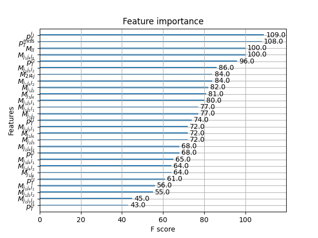
Figure 2: Ranking of the features used in the XGBOOST model training for the BLSM signal for the $2l+4j$ final state against the $t\bar{t}$(dileptonic) $+2j$ background.

We perform the training with events from the signal and the dominant $t\bar{t}$(dileptonic) $+2j$ background. Once the model is trained to distinguish between the BLSM signal and the $t\bar{t}$(dileptonic) $+2j$ background, we use it as a test on the events of the signal, the $t\bar{t}$(dileptonic) $+2j$, and the inclusive SM $2l4j$ background surviving the preliminary cuts. Fig. 2 shows the ranking of the various features according to their importance in making the classification decision, where the $F$ score is a measure of the relative importance of the variable. Among the most important features, we have the leading lepton $p_{T}$, the missing transverse momentum, the dileptonic invariant mass, and one combination of the $2j+l$ invariant mass, $M_{j_{1}j_{4}l_{1}}$.

Fig. 3 shows the distributions of some of the variables for the BLSM signal and the $t\bar{t}$(dileptonic) $+2j$. We observe that the $p_{T}^{l_{1}}$ and $M_{ll}$ distributions have longer tails for the BLSM $2l+4j$ signal as compared to the SM $t\bar{t}$(dileptonic) $+2j$ background, while the $p_{T}^{\rm miss}$ distribution for the latter is more likely to have higher values due to the neutrinos from the leptonic decay of the top quarks. Additionally, the distribution $M_{2l4j}$ peaks at the $Z^{\prime}$ boson mass of 3 TeV for the signal, while the minimum value of the various combinations for $M_{jjl}$ is sensitive to the $\nu_{R}$ mass with a peak around 400 GeV.

The distribution of the lepton charges show that in the BLSM signal, half of the events have same sign leptons due to the Majorana nature of the $\nu_{R}$, unlike the SM backgrounds. The charge of the lepton might get misidentified in the collider detectors while reconstruction. This will lead to a small fraction of same sign leptons even from the SM background. In this analysis, we have not used the lepton charges, since we don’t have the full parametrisation of the charge misidentification efficiency, which is dependent on the transverse momentum and pseudorapidity of the lepton. According to Ref. ATLAS:2019jvq , the misidentification efficiency for electrons is 0.1% in the central region, which increases to few percent for outer barrel region. The misidentification efficiency also increases with increasing lepton $p_{T}$. Using the lepton charge information would lead to better signal significance.

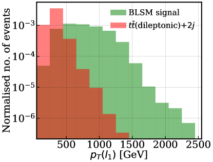
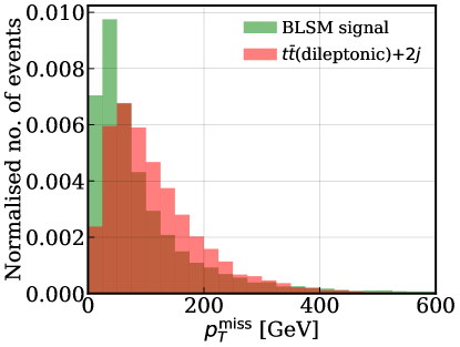
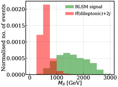
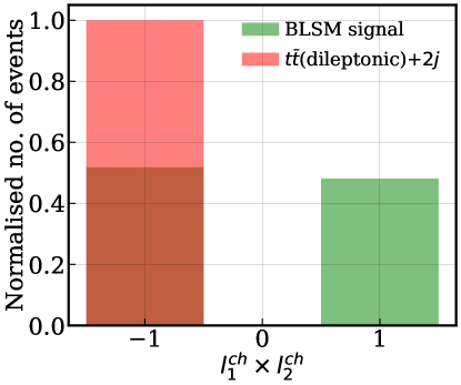
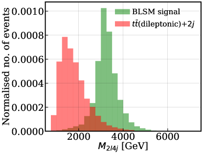
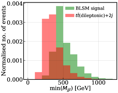
Figure 3: Normalised distributions of the transverse momenta of the leading lepton, $p_{T}^{l_{1}}$ (top left), the missing transverse momentum, $p_{T}^{\rm miss}$ (top right), the invariant mass of the dilepton system, $M_{ll}$ (centre left), the product of the two lepton charges (centre right), the invariant mass of the two leptons and the four jets, $M_{2l4j}$ (bottom left), and the minimum value from all the combinations of the invariant mass of the two jets and a lepton, min($M_{jjl}$) (bottom right) for the BLSM signal and the $t\bar{t}$(dileptonic) $+2j$.

Process		Cross-section (fb)	Events after XGBOOST score $>0.9$
Backgrounds	$t\bar{t}$ (leptonic) $+2j$	23.4	5.8
	$2l4j$	0.98	41.0
	Total	$-$	46.8
FS1		0.43	29.9
Significance $\left(\frac{S}{\sqrt{S+B}}\right)$		$-$	3.41

Table 3: Number of events from individual background processes and the signal surviving a threshold of 0.9 on the XGBOOST output from the model trained on our benchmark sample for the final state, FS1, along with the signal significance for $\mathcal{L}=3000$ fb^-1.

Table 3 shows the expected number of the BLSM signal benchmark for FS1 and the background events for a threshold of 0.9 on our XGBOOST output at $\sqrt{s}=14$ TeV LHC with 3000 fb^-1 of integrated luminosity ($\mathcal{L}$). We achieve a signal significance of 3.41.

4.2 FS2: $3l+2j+$ MET

The processes that we consider as the SM backgrounds for this final state are $-$ $WZ$(leptonic) $+2j$ and the $VVV$ processes, where $V$ is the $W$ or the $Z$ boson. We consider the inclusive $WWZ$, $ZZW$ and $ZZZ$ backgrounds $-$ a number of leptonic and hadronic decays of these vector bosons can constribute to this final state. Since the $\nu_{R}$’s coming from the decay of the 3 TeV $Z^{\prime}$ boson are highly boosted, the leptons from the same $\nu_{R}$ decay are very close to each other in the $\eta-\phi$ plane. We use the minimum cut on the $\Delta R$ between pairs of leptons to 0.1. We generate them using MG5 with the following cuts:

$$p_{T}^{l}>50\,{\rm GeV},~~~p_{T}^{j}>50\,{\rm GeV},~~~\Delta R(l,l)>0.1$$

While performing the Delphes detector simulation, we reduce the isolation cone of leptons to a radius of 0.1. We perform our analysis by putting the following preliminary cuts:

$$n_{l}=3,~~~p_{T}^{l}>50\,{\rm GeV},~~~|\eta^{l}|<2.5,$$

$$n_{j}>=2,~~~p_{T}^{j}>50\,{\rm GeV},~~~|\eta^{j}|<2.5\,{\rm GeV},~~~p_{T}^{\rm miss}>100\,{\rm GeV}$$

where $n_{l}$ and $n_{j}$ are the number of leptons and jets, respectively. We use the events surviving these cuts to train an XGBOOST model to classify between the signal and the background events. For the final state $3l+2j+$ MET, we have used the following variables to train the XGBOOST model:

• transverse momenta of the leptons and jets, $p_{T}^{l}$, $p_{T}^{j}$

• invariant mass of the two-jet system, $M_{jj}$

• various combinations of the invariant mass of the two leptons, $M_{ll}$ - this could be sensitive to the $\nu_{R}$ mass for the correct combination of the dileptons coming from the $\nu_{R}$ decay

• invariant mass of various combinations of two-jet systems with three of the leptons, $M_{jjl}$ - this could be sensitive to the $\nu_{R}$ mass for the correct combination of $2j+l$

• missing transverse energy, $p_{T}^{\rm miss}$

• transverse mass for each lepton with the MET, $M_{T}^{l}$

• invariant mass of the three leptons and two jets system, $M_{3l2j}$ - sensitive to the $Z^{\prime}$ mass

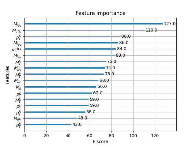
Figure 4: Ranking of the features used in the XGBOOST model training for the BLSM signal for the $3l+2j+$MET final state against the $WZ$(dileptonic) $+2j$ background.

We perform the training with events from the signal and the dominant $WZ$(leptonic) $+2j$ background. Once the model is trained, we use it as a test on the events of the signal, the $WZ$(leptonic) $+2j$, the inclusive $WWZ$, $ZZW$ and $ZZZ$ backgrounds surviving the preliminary analysis cuts. Fig. 4 shows the ranking of the various features according to their importance in making the classification decision. Among the most important features, we have $M_{l_{2}l_{3}}$ and $M_{3l2j}$, which are sensitive to the $\nu_{R}$ and the $Z^{\prime}$ boson masses, respectively.

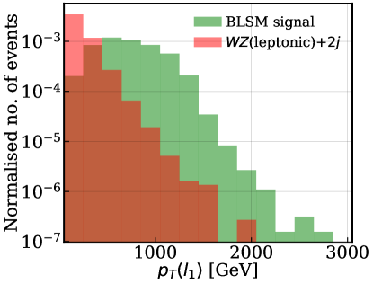
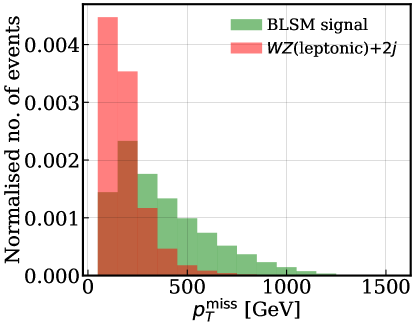
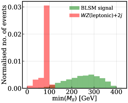
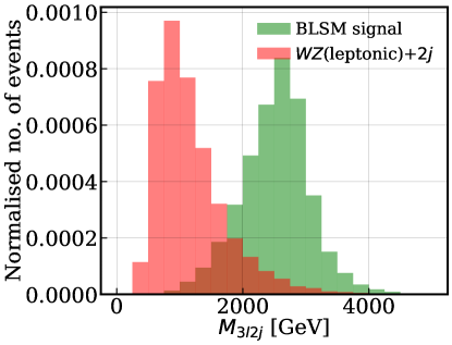
Figure 5: Normalised distributions of the transverse momenta of the leading lepton, $p_{T}^{l_{1}}$ (top left), the missing transverse momentum, $p_{T}^{\rm miss}$ (top right), the invariant mass of one of the dilepton systems, $M_{l_{2}l_{3}}$ (bottom left), and the invariant mass of the three leptons and the two jets, $M_{3l2j}$ (bottom right) for the BLSM signal and the $WZ$(leptonic) $+2j$.

Fig. 5 shows the distributions of some of the variables for the BLSM signal and the $WZ$(leptonic) $+2j$. We observe that the $p_{T}^{l_{1}}$ and $p_{T}^{\rm miss}$ distributions have longer tails for the BLSM $3l+2j+$MET signal as compared to the SM $WZ$(leptonic) $+2j$ background. Additionally, the distribution $M_{3l2j}$ peaks around the $Z^{\prime}$ boson mass of 3 TeV for the signal, while the distribution of the minimum value of the combination $M_{ll}$ is sensitive to the $\nu_{R}$ mass, falling sharply around 400 GeV.

Process		Cross-section (fb)	Events after XGBOOST score $>0.9$
Backgrounds	$WZ$ (leptonic) $+2j$	13.98	1.1
	$WWZ$	94.2	0
	$ZZW$	30.3	0
	$ZZZ$	10.3	0
	Total	$-$	1.1
FS2		0.43	66.2
Significance $\left(\frac{S}{\sqrt{S+B}}\right)$		$-$	8.07

Table 4: Number of events from individual background processes and the signal surviving a threshold of 0.9 on the XGBOOST output from the model trained on our benchmark sample for the final state, FS2 along with the signal significance for $\mathcal{L}=3000$ fb^-1.

Table 4 shows the expected number of the BLSM signal benchmark for FS2 and the background events for a threshold of 0.9 on our XGBOOST output at $\sqrt{s}=14$ TeV LHC with 3000 fb^-1 of integrated luminosity ($\mathcal{L}$). We achieve a signal significance of 8.07.

4.3 FS3: $4l+$ MET

The processes that we consider as the SM backgrounds for this final state are the $VVV$ processes, where $V$ is the $W$ or the $Z$ boson. We consider the inclusive $WWZ$, $ZZW$ and $ZZZ$ backgrounds. This final state is pretty clean due to the presence of four high $p_{T}$ leptons, and we only perform a cut-based analysis. The leptons coming from the decay chain of a single $\nu_{R}$ are again very close to each other in the $\eta-\phi$ plane. We use a value of 0.1 for the isolation cone of the leptons in our Delphes analysis. We perform our analysis by putting the following cuts:

$$n_{l}=4,~~~p_{T}^{l}>50\,{\rm GeV},~~~|\eta^{l}|<2.5,~~~p_{T}^{\rm miss}>100\,{\rm GeV}.$$

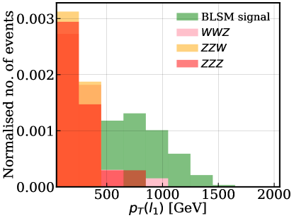
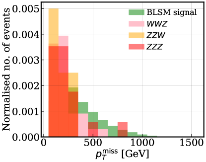
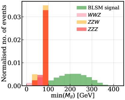
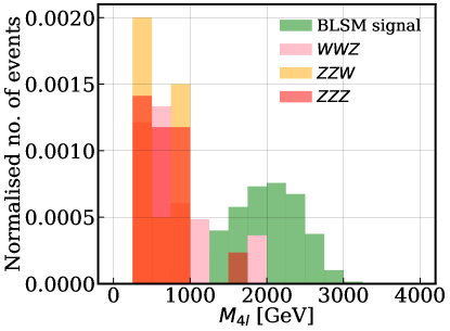
Figure 6: Normalised distributions of the transverse momenta of the leading lepton, $p_{T}^{l_{1}}$ (top left), the missing transverse momentum, $p_{T}^{\rm miss}$ (top right), the invariant mass of one of the dilepton systems, $M_{l_{2}l_{3}}$ (bottom left), and the invariant mass of the three leptons and the two jets, $M_{3l2j}$ (bottom right) for the BLSM signal and the $WZ$(leptonic) $+2j$.

Fig. 6 shows the distributions of some of the variables for the BLSM signal and the $VVV$ backgrounds. We observe that the $p_{T}^{l_{1}}$ and $p_{T}^{\rm miss}$ distributions have longer tails for the BLSM $4l+$MET signal as compared to the SM triboson backgrounds. Additionally, the edge of the distribution of the minimum value from all the combinations for $M_{ll}$ around 400 GeV is sensitive to the $\nu_{R}$ mass. Similarly, the $M_{4l}$ distribution has a edge at 3 TeV, which is the mass of the $Z^{\prime}$ boson for the signal benchmark.

Process		Cross-section (fb)	Events after cuts
Backgrounds	$WWZ$	94.2	18.6
	$ZZW$	30.3	1.4
	$ZZZ$	10.3	1.0
	Total	$-$	21.0
FS3		0.109	37.6
Significance $\left(\frac{S}{\sqrt{S+B}}\right)$		$-$	4.91

Table 5: Number of events from individual background processes and the signal surviving the analysis cuts for the final state, FS3, along with the signal significance for $\mathcal{L}=3000$ fb^-1.

Table 5 shows the expected number of the BLSM signal benchmark for FS2 and the background events passing the analysis cuts at $\sqrt{s}=14$ TeV LHC with 3000 fb^-1 of integrated luminosity ($\mathcal{L}$). We achieve a signal significance of 4.91.

5 Conclusions

The $B-L$ extension of the SM of particle physics naturally explains the observed small masses of left-handed neutrinos. Searches for signatures of the new particles arising in BLSM, like the $Z^{\prime}$ gauge boson and RHNs, have been performed by experimental collaborations. These searches put bounds on the couplings and masses of these particles. In the present study, we investigate the prospect of analyses based on the XGBOOST machine learning framework at the HL-LHC for a BLSM benchmark which is not yet excluded by the present experiments. We consider production of the $Z^{\prime}$ boson from proton-proton collisions, which further decay into RHNs. For RHNs, we consider their decay to a lepton and $W$ bosons. The fully hadronic, semi-leptonic and fully leptonic decays of the two $W$ bosons are analysed and classified from various SM background processes. For each of the three final states, we find that at the HL-LHC, we can achieve a signal significance greater than $3\sigma$ with the analyses presented in this work. We find that a cut based analysis is enough to probe the BLSM signal with the $4l+$MET final state, however, for the other two final states, the XGBOOST classification provides better sensitivity. In conclusion, the analyses performed in this study are sensitive probes of the BLSM signatures at the LHC.

Appendix A Details of the XGBOOST model

We train our XGBOOST model using the following hyperparameters:

‘objective’:‘multi:softprob’,‘colsample_bytree’:0.3,‘colsample_bylevel’:0.3,
‘colsample_bynode’:0.3,‘learning_rate’: 0.1,‘num_class’:2,
‘max_depth’: 3, ‘lambda’: 5, ‘alpha’: 5, ‘gamma’: 2,

We divide our total sample in two parts $-$ one for training and one for validation.

References

- (1) Super-Kamiokande Collaboration, Y. Fukuda et al., “Evidence for oscillation of atmospheric neutrinos,” Phys. Rev. Lett. 81 (1998) 1562–1567, arXiv:hep-ex/9807003.
- (2) K2K Collaboration, M. Ahn et al., “Indications of neutrino oscillation in a 250 km long baseline experiment,” Phys. Rev. Lett. 90 (2003) 041801.
- (3) KamLAND Collaboration, K. Eguchi et al., “First results from KamLAND: Evidence for reactor anti-neutrino disappearance,” Phys. Rev. Lett. 90 (2003) 021802.
- (4) SNO Collaboration, Q. Ahmad et al., “Direct evidence for neutrino flavor transformation from neutral current interactions in the Sudbury Neutrino Observatory,” Phys. Rev. Lett. 89 (2002) 011301.
- (5) Daya Bay Collaboration, F. An et al., “Observation of electron-antineutrino disappearance at Daya Bay,” Phys. Rev. Lett. 108 (2012) 171803.
- (6) R. N. Mohapatra and R. E. Marshak, “Local B-L Symmetry of Electroweak Interactions, Majorana Neutrinos and Neutron Oscillations,” Phys. Rev. Lett. 44 (1980) 1316–1319. [Erratum: Phys.Rev.Lett. 44, 1643 (1980)].
- (7) A. Papaefstathiou, “Phenomenological aspects of new physics at high energy hadron colliders,” other thesis, 8, 2011.
- (8) A. Masiero, J. F. Nieves, and T. Yanagida, “B-L Violating Proton Decay and Late Cosmological Baryon Production,” Phys. Lett. B 116 (1982) 11–15.
- (9) R. N. Mohapatra and G. Senjanovic, “Spontaneous Breaking of Global B-L Symmetry and Matter - Antimatter Oscillations in Grand Unified Theories,” Phys. Rev. D 27 (1983) 254.
- (10) W. Buchmuller, C. Greub, and P. Minkowski, “Neutrino masses, neutral vector bosons and the scale of B-L breaking,” Phys. Lett. B 267 (1991) 395–399.
- (11) S. Khalil, “Low scale - L extension of the Standard Model at the LHC,” J. Phys. G 35 (2008) 055001, arXiv:hep-ph/0611205.
- (12) W. Emam and S. Khalil, “Higgs and Z-prime phenomenology in B-L extension of the standard model at LHC,” Eur. Phys. J. C 52 (2007) 625–633, arXiv:0704.1395 [hep-ph].
- (13) S. Khalil, “TeV-scale gauged B-L symmetry with inverse seesaw mechanism,” Phys. Rev. D 82 (2010) 077702, arXiv:1004.0013 [hep-ph].
- (14) A. A. Abdelalim, A. Hammad, and S. Khalil, “B-L heavy neutrinos and neutral gauge boson Z’ at the LHC,” Phys. Rev. D 90 no. 11, (2014) 115015, arXiv:1405.7550 [hep-ph].
- (15) “XGBOOST Documentation.” https://xgboost.readthedocs.io/en/stable/.
- (16) L.-G. Xia, “Understanding the boosted decision tree methods with the weak-learner approximation,” arXiv:1811.04822 [physics.data-an].
- (17) L.-G. Xia, “Qbdt, a new boosting decision tree method with systematical uncertainties into training for high energy physics,” Nuclear Instruments and Methods in Physics Research Section A: Accelerators, Spectrometers, Detectors and Associated Equipment 930 (2019) 15–26. https://www.sciencedirect.com/science/article/pii/S0168900219304309.
- (18) J. R. Quinlan, “Induction of decision trees,” Machine Learning 1 no. 1, (1986) 81–106.
- (19) J. R. Quinlan, “Simplifying decision trees,” International Journal of Man-Machine Studies 27 no. 3, (1987) 221–234.
- (20) M. Carena, A. Daleo, B. A. Dobrescu, and T. M. P. Tait, “ gauge bosons at the Tevatron,” Phys. Rev. D 70 (2004) 093009, arXiv:hep-ph/0408098.
- (21) CDF Collaboration, A. Abulencia et al., “Search for using dielectron mass and angular distribution.,” Phys. Rev. Lett. 96 (2006) 211801, arXiv:hep-ex/0602045.
- (22) A. Collaboration, “Search for high-mass dilepton resonances using of pp collision data at tev with the atlas detector,” Physical Review Letters 123 no. 16, (2019) 161801.
- (23) A. Leike, “The phenomenology of extra neutral gauge bosons,” Physics Reports 317 (1999) 143–250.
- (24) P. Langacker, “The physics of heavy gauge bosons,” Reviews of Modern Physics 81 (2009) 1199–1228.
- (25) H. L. Lai, J. Botts, J. Huston, J. G. Morfin, J. F. Owens, J. W. Qiu, W. K. Tung, and H. Weerts, “Global qcd analysis and the cteq parton distributions,” Physical Review D 51 (1995) 4763–4782.
- (26) R. D. Ball, V. Bertone, F. Cerutti, L. D. Debbio, S. Forte, A. Guffanti, J. Rojo, and M. Ubiali, “Parton distributions for the lhc run ii,” Journal of High Energy Physics 2015 no. 04, (2015) 040.
- (27) CMS Collaboration, V. Khachatryan et al., “Performance of Electron Reconstruction and Selection with the CMS Detector in Proton-Proton Collisions at s = 8 TeV,” JINST 10 no. 06, (2015) P06005, arXiv:1502.02701 [physics.ins-det].
- (28) CMS Collaboration, A. M. Sirunyan et al., “Performance of the CMS muon detector and muon reconstruction with proton-proton collisions at 13 TeV,” JINST 13 no. 06, (2018) P06015, arXiv:1804.04528 [physics.ins-det].
- (29) ATLAS Collaboration, M. Aaboud et al., “Electron reconstruction and identification in the ATLAS experiment using the 2015 and 2016 LHC proton-proton collision data at = 13 TeV,” Eur. Phys. J. C 79 no. 8, (2019) 639, arXiv:1902.04655 [physics.ins-det].
- (30) F. Staub, “Sarah 4: A tool for (not only susy) model builders,” Computer Physics Communications 185 (2014) 1773–1790, arXiv:1309.7223 [hep-ph].
- (31) W. Porod, “Spheno, a program for calculating supersymmetric spectra, susy particle decays and susy particle production at colliders,” Computer Physics Communications 153 (2003) 275–315.
- (32) J. Alwall, R. Frederix, S. Frixione, V. Hirschi, F. Maltoni, O. Mattelaer, H. M. P. Victoria, T. Plehn, M. Schumann, S. Alioli, and J. R. Andersen, “The automated computation of tree-level and next-to-leading order differential cross sections, and their matching to parton shower simulations,” Journal of High Energy Physics 2014 no. 7, (2014) 79, arXiv:1405.0301 [hep-ph].
- (33) J. de Favereau, C. Delaere, P. Demin, A. Giammanco, V. Lemaître, A. Mertens, and M. Selvaggi, “Delphes 3: A modular framework for fast simulation of a generic collider experiment,” Journal of High Energy Physics 2014 no. 2, (2014) 57, arXiv:1307.6346 [hep-ex].