Gravitational Waves from Post-Collision of Fuzzy Dark Matter Solitons

Abstract

According to the Schrödinger-Poisson (SP) equations, fuzzy dark matter (FDM) can form a stable equilibrium configuration, the so-called FDM soliton. The SP system can also determine the evolution of FDM solitons, such as head-on collision. In this paper, we first propose a new adimensional unit of length, time and mass. And then, we simulate the adimensional SP system with $\mathtt{PyUltraLight}$ to study the GWs from post-collision of FDM solitons when the linearized theory is valid and the GW back reaction on the evolution of FDM solitons is ignored. Finally, we find that the GWs from post-collisions have a frequency of (few ten-years)^-1 or (few years)^-1 when FDM mass is $m=10^{-18}\rm{eV}/c^{2}$ or $m=10^{-17}\rm{eV}/c^{2}$. Therefore, future detection of such GWs will constrain the property of FDM particle and solitons.

I Introduction

Gravitational waves (GWs) are ripples in spacetime. Einstein’s general relativity predicts that this kind of gravitational radiation involves a spherically or rotationally asymmetric acceleration among the masses. More precisely, an isolated system will radiate GWs when the second (or third, …) time derivative of the quadrupole (or octupole, …) moment of its stress–energy tensor is nonzero. The Universe is expected to be populated by GWs spanning orders of magnitude in frequency. For example, $\gtrsim 10^{-16}$Hz primordial GWs due to primordial tensor fluctuations during cosmic inflation left their footprints in the B-modes polarization anisotropies of the cosmic microwave background radiation (CMB), which is allegedly detected by CMB polarization telescope BICEP:2021xfz ; Li:2017drr ; binary supermassive black holes in galactic nuclei emit about $10^{-8}-10^{-3}$Hz GWs, whose low-frequency end is supposed to be detected by pulsar timing arrays NANOGrav:2023gor ; EPTA:2023fyk ; Reardon:2023gzh ; compact binaries or black hole binaries in galaxies emit about $10^{-3}-10^{3}$Hz GWs during their inspiral, merger and ring-down phases, whose low-frequency end would be detected by future space-based interferometers LISA:2017pwj ; Hu:2017mde ; TianQin:2015yph and whose high-frequency end can be detected by ground-based interferometers KAGRA:2021vkt ; LIGOScientific:2020ibl ; LIGOScientific:2018mvr ; GWs at frequencies higher than $10$kHz are proposed to be sourced by some phenomenons involving beyond the Standard Model physics, such as preheating after inflation Khlebnikov:1997di ; Easther:2006gt ; Garcia-Bellido:2007fiu and phase transitions at high energies in the early Universe Grojean:2006bp ; Hindmarsh:2015qta ; Hindmarsh:2013xza ; Kosowsky:1992rz , which prompt many new detector concepts in the laboratory Aggarwal:2020olq . What interesting astrophysical objects or cosmological events can source GWs in the $\lesssim 10^{-8}$Hz frequency range?

As a promising candidate for dark matter Rubin:1982kyu ; Davis:1985rj ; Clowe:2006eq , the ultralight scalar field with spin-$0$, extraordinarily light mass ($m\sim 10^{-22}\rm{eV}/c^{2}$) and de Broglie wavelength comparable to a few kpc, namely fuzzy dark matter (FDM) Hu:2000ke , can form an equilibrium configuration with size smaller than its de Broglie wavelength, the so-called FDM soliton Guzman:2004wj ; Davies:2019wgi . The subsequent evolutions of FDM solitons are usually simulated numerically, including the perturbation, the interference/collision and the tidal disruption/deformation of FDM solitons Guzman:2004wj ; Paredes:2015wga ; Edwards:2018ccc ; Munive-Villa:2022nsr , according to the coupled Schrödinger–Poisson (SP) system of equations

$$\begin{cases}\begin{aligned} &i\hbar\frac{\partial\Psi}{\partial t}=\left(-\frac{\hbar^{2}}{2m}\nabla^{2}+m\Phi\right)\Psi,\\ &\nabla^{2}\Phi=4\pi Gm|\Psi|^{2},\end{aligned}\end{cases}$$ (1)

where FDM is described by the wavefunction $\Psi$, $m$ is the mass of FDM and the gravitational potential $\Phi$ is sourced by the FDM density $\rho=|\Psi|^{2}$. Because of the large size of the FDM solitions and the weak self-gravitational potential, it is hard to form gravitational bound systems between FDM solitons, such as binary FDM solitons. Even though without the normal inspiral, merger and ring-down phases of a compact binary system, the other spherically or rotationally asymmetric evolutions of FDM solitons should also emit GWs. As shown in this paper, for example, since the size of the FDM soliton is typically on the order of kpc, the frequency of GWs emitted from post-collision of FDM solitons is typically on the order of c/kpc$\sim 10^{-11}$Hz. The mass $m$ of the FDM particle or the velocity $v$ and mass $M$ of the FDM solitons can further be fine-tuned to adjust the frequency of such GWs. In other words, future detection of such GWs can constrain the property of the FDM particle and the FDM solitons.

However, gravitational radiation carries away the energy and momentum of isolated systems. Therefore, in principle, the SP system (Eq. (1)) should be enlarged by including the wave equation for GWs $h_{\mu\nu}$

$$\square h_{\mu\nu}=-\frac{16\pi G}{c^{4}}T_{\mu\nu},$$ (2)

where $T_{\mu\nu}$ is the energy-momentum tensor of FDM solitons and we have assumed that the linearized theory is valid because that the SP system is nothing but the weak field limit of its general relativistic counterpart, the Einstein–Klein–Gordon (EKG) system Kaup:1968zz ; Ruffini:1969qy ; Ma:2023vfa . Furthermore, the GW back reaction on FDM solitons will modify Eq. (1). As the system’s energy is carried away by GWs, the FDM solitons would settle down gradually and eventually. However, if the gravitational radiation is not efficient, the GW back reaction on the evolution of FDM solitons can be neglected approximately, which is done in this paper.

This paper is organized as follows. In Section II, we turn to the shooting method to solve the SP system (Eq. (1)) and obtain the isolated FDM solitons. In Section III, we numerically simulate the evolution of FDM solitons with $\mathtt{PyUltraLight}$ Edwards:2018ccc , the post-collision of FDM solitons in particular. In Section IV, we calculate the waveform of GWs emitted from post-collision of FDM solitons. Finally, a brief summary and discussions are included in Section V.

II Fuzzy Dark Matter Solitons

Before the numerical simulation of the evolution of FDM solitons, we should first build up the profile of an isolated FDM soliton. Since an isolated FDM soliton features spherical symmetry, the ansatz of $\Psi(r,t)=e^{i\gamma t}\psi(r)$ means that the FDM particle number density is $|\Psi|^{2}$, the FDM soliton density is $\rho(r)=m|\Psi|^{2}=m\psi^{2}(r)$ and the FDM soliton mass is $M=\int_{0}^{\infty}4\pi r^{2}\rho(r)dr$. After defining a number of dimensionless variables as

$$\tilde{r}\equiv\frac{mc}{\hbar}r,$$

$$\tilde{t}\equiv\frac{mc^{2}}{\hbar}t,$$

$$\tilde{\psi}\equiv\frac{\hbar\sqrt{G}}{c^{2}\sqrt{m}}\psi,$$

$$\tilde{\Phi}\equiv\frac{1}{c^{2}}\Phi,$$

$$\tilde{\gamma}\equiv\frac{\hbar}{mc^{2}}\gamma,$$

$$\tilde{M}\equiv\frac{Gm}{\hbar c}M,$$ (3)

the dimensionless spatial part of Eq. (1) is

$$\begin{cases}\begin{aligned} &\frac{\partial^{2}(\tilde{r}\tilde{\psi})}{\partial\tilde{r}^{2}}=2\tilde{r}\left(\tilde{\Phi}+\tilde{\gamma}\right)\tilde{\psi},\\ &\frac{\partial^{2}(\tilde{r}\tilde{\Phi})}{\partial\tilde{r}^{2}}=4\pi\tilde{r}\tilde{\psi}^{2}.\end{aligned}\end{cases}$$ (4)

Fulfilling arbitrary normalization $\tilde{\psi}(\tilde{r}=0)=1$ and boundary conditions $\tilde{\Phi}(\tilde{r}=\infty)=0$, $\tilde{\psi}(\tilde{r}=\infty)=0$, $\frac{\partial\tilde{\psi}}{\partial\tilde{r}}|_{\tilde{r}=0}=0$ and $\frac{\partial\tilde{\Phi}}{\partial\tilde{r}}|_{\tilde{r}=0}=0$ and adjusting the quantized eigenvalue $\tilde{\gamma}$, we can calculate the equilibrium configurations from Eq. (1) by the shooting method. Only the solution from the smallest $\tilde{\gamma}$ is stable and the ground state. We also obtain the first excited state. In Tab. 1, we list the eigenvalues $\tilde{\gamma}$ and soliton masses $\tilde{M}$ of the ground state and the first excited state. In Fig. 1, the corresponding soliton profiles are plotted. Since the SP system (Eq. (4)) has the scaling symmetry

$$\tilde{r}\longrightarrow\lambda^{-1/2}\tilde{r},$$

$$\tilde{\psi}\longrightarrow\lambda\tilde{\psi},$$

$$\tilde{\Phi}\longrightarrow\lambda\tilde{\Phi},$$

$$\tilde{\gamma}\longrightarrow\lambda\tilde{\gamma},$$

$$\tilde{M}\longrightarrow\lambda^{1/2}\tilde{M},$$ (5)

we can adjust the mass of FDM solitons with $\lambda$ to set up different initial conditions for collision.

Table 1: Eigenvalues $\tilde{\gamma}$ and masses $\tilde{M}$ of the ground state and the first excited state.

Nodes	$\tilde{\gamma}$	$\tilde{M}$
0	2.45	3.88
1	2.30	8.64

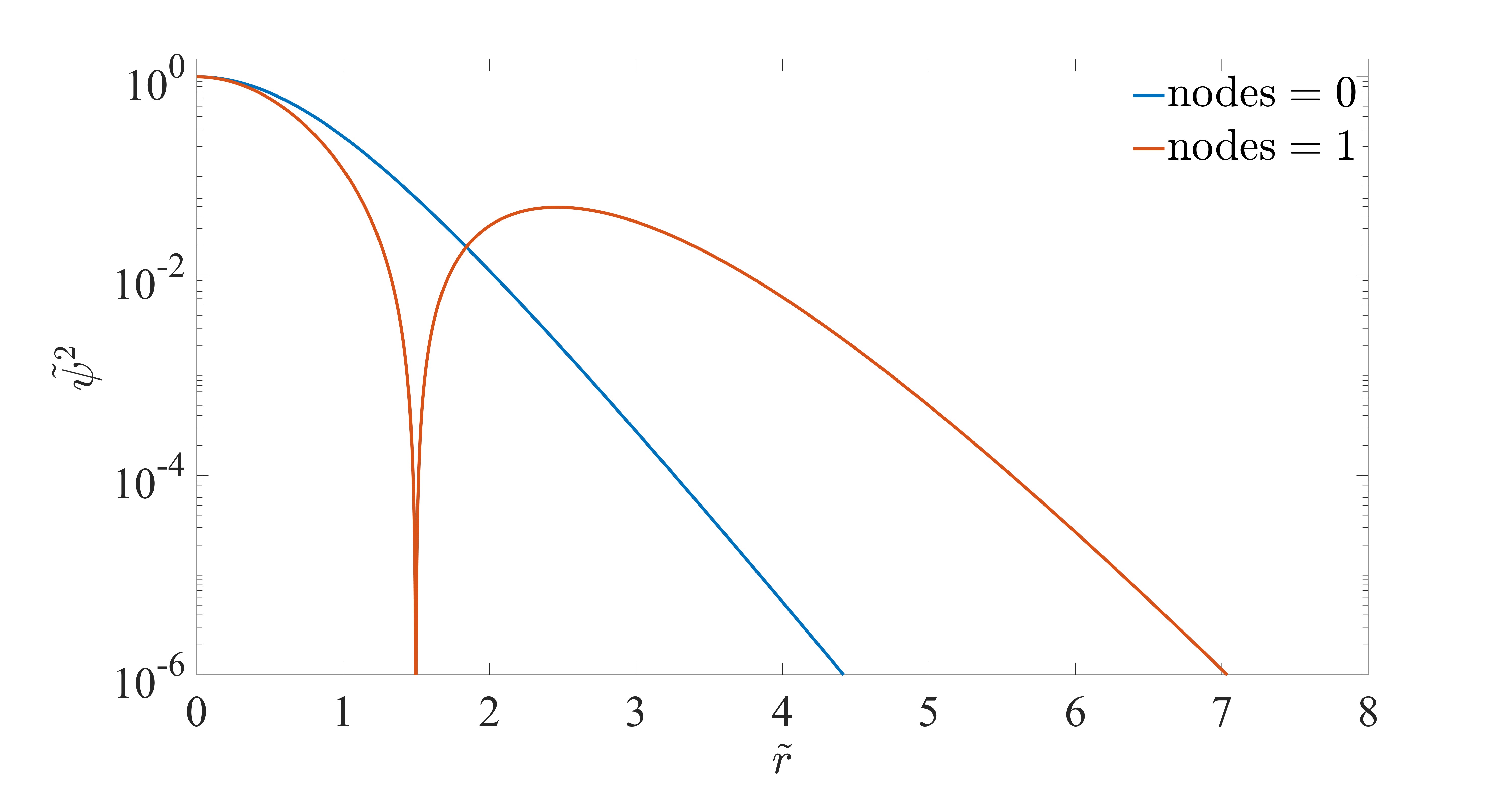
(a)

Figure 1: Density profiles of the ground state (blue curve) and the first excited state (orange curve).

Summarizing Eq. (II), we can introduce the length, time and mass scales as follows

$$\mathcal{L}\equiv\frac{\hbar}{mc}\approx 6.39\times 10^{-5}\left(\frac{10^{-22}\rm{eV}/c^{2}}{m}\right)\rm{kpc},$$

$$\mathcal{T}\equiv\frac{\hbar}{mc^{2}}\approx 6.57\times 10^{6}\left(\frac{10^{-22}\rm{eV}/c^{2}}{m}\right)\rm{s},$$

$$\mathcal{M}\equiv\frac{\hbar c}{Gm}\approx 1.34\times 10^{12}\left(\frac{10^{-22}\rm{eV}/c^{2}}{m}\right)\rm{M}_{\odot}.$$ (6)

Since, for example, the mass of an isolated soliton $M$ can be predicted from the halo mass $M_{\rm{halo}}$ according to the soliton-halo mass relation Schive:2014hza

$$M \approx 1.25\times 10^{9}\left(\frac{M_{\rm{halo}}}{10^{12}\rm{M}_{\odot}}\right)^{1/3}\left(\frac{m}{10^{-22}{\rm{eV}}/c^{2}}\right)^{-1}\rm{M}_{\odot}$$

$$\approx 9.33\times 10^{-4}\left(\frac{M_{\rm{halo}}}{10^{12}\rm{M}_{\odot}}\right)^{1/3}\mathcal{M},$$ (7)

for the ground state, we have

$$\lambda\approx 5.78\times 10^{-8}\left(\frac{M_{\rm{halo}}}{10^{12}\rm{M}_{\odot}}\right)^{2/3};$$ (8)

for the first excited state, we have

$$\lambda\approx 1.17\times 10^{-8}\left(\frac{M_{\rm{halo}}}{10^{12}\rm{M}_{\odot}}\right)^{2/3}.$$ (9)

Then, for a more general system of FDM solitons, we can obtain a number of dimensionless variables including the spatial position, time and the wavefunction, gravitational potential, eigenvalue, mass, density, energy Edwards:2018ccc and velocity of FDM solitons respectively as

$$\tilde{\vec{x}}=\frac{\vec{x}}{\mathcal{L}},$$

$$\tilde{t}=\frac{t}{\mathcal{T}},$$

$$\tilde{\Psi}=\mathcal{T}\sqrt{mG}\Psi,$$

$$\tilde{\Phi}=\frac{m\mathcal{T}}{\hbar}\Phi,$$

$$\tilde{\gamma}=\mathcal{T}\gamma,$$

$$\tilde{M}=\frac{M}{\mathcal{M}}=\int d^{3}\tilde{x}|\tilde{\Psi}|^{2},$$

$$\tilde{\rho}=\frac{\rho}{\mathcal{ML}^{-3}}=|\tilde{\Psi}|^{2},$$

$$\tilde{E}=\frac{E}{\mathcal{ML}^{2}\mathcal{T}^{-2}}=\int d^{3}x\left(\frac{1}{2}\tilde{\Phi}|\tilde{\Psi}|^{2}-\frac{1}{2}\tilde{\Psi}^{*}\nabla^{2}\tilde{\Psi}\right),$$

$$\tilde{\vec{v}}=\frac{\vec{v}}{\mathcal{L}\mathcal{T}^{-1}}.$$ (10)

Finally, the dimensionless version of Eq. (1) without any assumption of spatial symmetry is

$$\begin{cases}\begin{aligned} &i\frac{\partial\Psi(\vec{x},t)}{\partial t}=\left(-\frac{1}{2}\nabla^{2}+\Phi(\vec{x},t)\right)\Psi(\vec{x},t),\\ &\nabla^{2}\Phi(\vec{x},t)=4\pi|\Psi(\vec{x},t)|^{2},\end{aligned}\end{cases}$$ (11)

where we have dropped the tildes for notational convenience until Section IV.

III Collision of Fuzzy Dark Matter Solitons

In this paper, we numerically simulate the evolution of FDM solitons with $\mathtt{PyUltraLight}$ Edwards:2018ccc , the post-collision of FDM solitons in particular. $\mathtt{PyUltraLight}$ is designed to solve the SP system under periodic boundary conditions. Then, Eq. (11) should be rewrite as

$$\begin{cases}\begin{aligned} &i\frac{\partial\Psi(\vec{x},t)}{\partial t}=\left(-\frac{1}{2}\nabla^{2}+\Phi(\vec{x},t)\right)\Psi(\vec{x},t),\\ &\nabla^{2}\Phi(\vec{x},t)=4\pi(|\Psi(\vec{x},t)|^{2}-\langle|\Psi(\vec{x},t)|^{2}\rangle),\end{aligned}\end{cases}$$ (12)

where $\langle|\Psi(\vec{x},t)|^{2}\rangle$ is the average density over the simulation box. After a sufficiently small timestep $\Delta t$, $\mathtt{PyUltraLight}$ evolves $\Psi(\vec{x},t)$ and $\Phi(\vec{x},t)$ in Eq. (12) as

$$\begin{cases}\begin{aligned} \Psi(\vec{x},t+\Delta t/2)&=\mathcal{F}^{-1}\exp\left[-\frac{i\Delta t}{2}k^{2}\right]\mathcal{F}\\ &\times\exp\left[-\frac{i\Delta t}{2}\Phi(\vec{x},t)\right]\Psi(\vec{x},t),\\ \Phi(\vec{x},t+\Delta t)&=\mathcal{F}^{-1}\left(-\frac{1}{k^{2}}\right)\mathcal{F}4\pi|\Psi(\vec{x},t+\Delta t/2)|^{2},\\ \Psi(\vec{x},t+\Delta t)&=\exp\left[-\frac{i\Delta t}{2}\Phi(\vec{x},t+\Delta t)\right]\Psi(\vec{x},t+\Delta t/2),\end{aligned}\end{cases}$$ (13)

where the order of operations runs from right to left, $\mathcal{F}$ and $\mathcal{F}^{-1}$ denote the discrete Fourier transform and its inverse, $k$ is the wavenumber in the Fourier domain and the global average density disappears. For the collision of two FDM solitions, the initial total wavefunction is

$$\Psi(\vec{x},t_{0})=\sum_{n=1}^{2} \left[\lambda_{n}\psi(\sqrt{\lambda_{n}}|\vec{x}-\vec{x}_{n}-\vec{v}_{n}t_{0}|)~{}\times\right.$$

$$\left.e^{i(\lambda_{n}\gamma_{n}t_{0}+\vec{v}_{n}\cdot(\vec{x}-\vec{x}_{n})-\frac{1}{2}|\vec{v}_{n}|^{2}t_{0}+\delta_{n})}\right],$$ (14)

where $\lambda_{n}$ rescales the initial masse and size of FDM soliton according to Eq. (II), $\gamma_{n}$ is the soliton eigenvalue (or $\lambda_{n}\gamma_{n}$ is its rescaled counterpart), $\vec{x}_{n}$ is the initial central position of the FDM solition, $\vec{v}_{n}$ is the FDM soliton velocity, $\delta_{n}$ is the initial phase and $t_{0}$ is the start time. Given $t_{0}=0$, the simulation resolution $N^{3}=256^{3}$ and the length of simulation box $l=2\times 10^{4}$, we can study the dynamics of the FDM solitons collision. In Tab. 2, we list the setup for $3$ head-on collisions, namely C$1$, C$2$ and C$3$.

Table 2: Setup for $3$ head-on collisions, where $\gamma_{n}$ decides the initial density profile according to Tab. 1 and Fig. 1 and $\lambda_{n}$ is related to its corresponding $M_{\rm{halo}}$ as Eq. (8) or Eq. (9).

Collision	$\lambda_{1}$	$\gamma_{1}$	$\delta_{1}$	$\vec{x}_{1}$	$\vec{v}_{1}$
C$1$	$1.66\times 10^{-6}$	$2.45$	$0$	$\left(\frac{l}{4},0,0\right)$	$\left(10^{-4},0,0\right)$
C$2$	$1.66\times 10^{-6}$	$2.45$	$0$	$\left(\frac{l}{4},0,0\right)$	$\left(10^{-4},0,0\right)$
C$3$	$1.66\times 10^{-6}$	$2.45$	$0$	$\left(\frac{l}{4},0,0\right)$	$\left(10^{-4},0,0\right)$
Collision	$\lambda_{2}$	$\gamma_{2}$	$\delta_{2}$	$\vec{x}_{2}$	$\vec{v}_{2}$
C$1$	$1.66\times 10^{-6}$	$2.45$	$0$	$\left(\frac{3l}{4},0,0\right)$	$\left(-10^{-4},0,0\right)$
C$2$	$4.15\times 10^{-7}$	$2.45$	$0$	$\left(\frac{3l}{4},0,0\right)$	$\left(-10^{-4},0,0\right)$
C$3$	$1.34\times 10^{-6}$	$2.30$	$0$	$\left(\frac{3l}{4},0,0\right)$	$\left(0,0,0\right)$

During simulations, energy conservation should be guaranteed. As shown in Eq. (II), the total energy can be decomposed into the kinetic energy $E_{\rm{k}}$ and the gravitational potential energy $E_{\rm{p}}$ when the GW back reaction is ignored. In the left subplots of Fig. 2, Fig. 3 and Fig. 4, we find that energy conservation is satisfied. In the right subplots of Fig. 2, Fig. 3 and Fig. 4, we show the evolutions of FDM sollitons for head-on collision. We find that $E_{\rm{p}}$ is large enough to merge the initial two FDM solitons with each other after collisions; the energy transfer between $E_{\rm{k}}$ and $E_{\rm{p}}$ causes the final FDM soliton to oscillate irregularly with an adimensional frequency of $\sim 10^{-8}$; the location of merger depends on system’s mass-ratio. Especially for C3, the mass-ratio between one FDM soliton with the density profile as the ground state and another with the density profile as the first excited state is $0.5$ but the larger one without initial velocity is attracted away from its initial position, as shown in the right subplot of Fig. 4. It means that the FDM soliton with the density profile as the first excited state is not stable and is dismembered before collision.

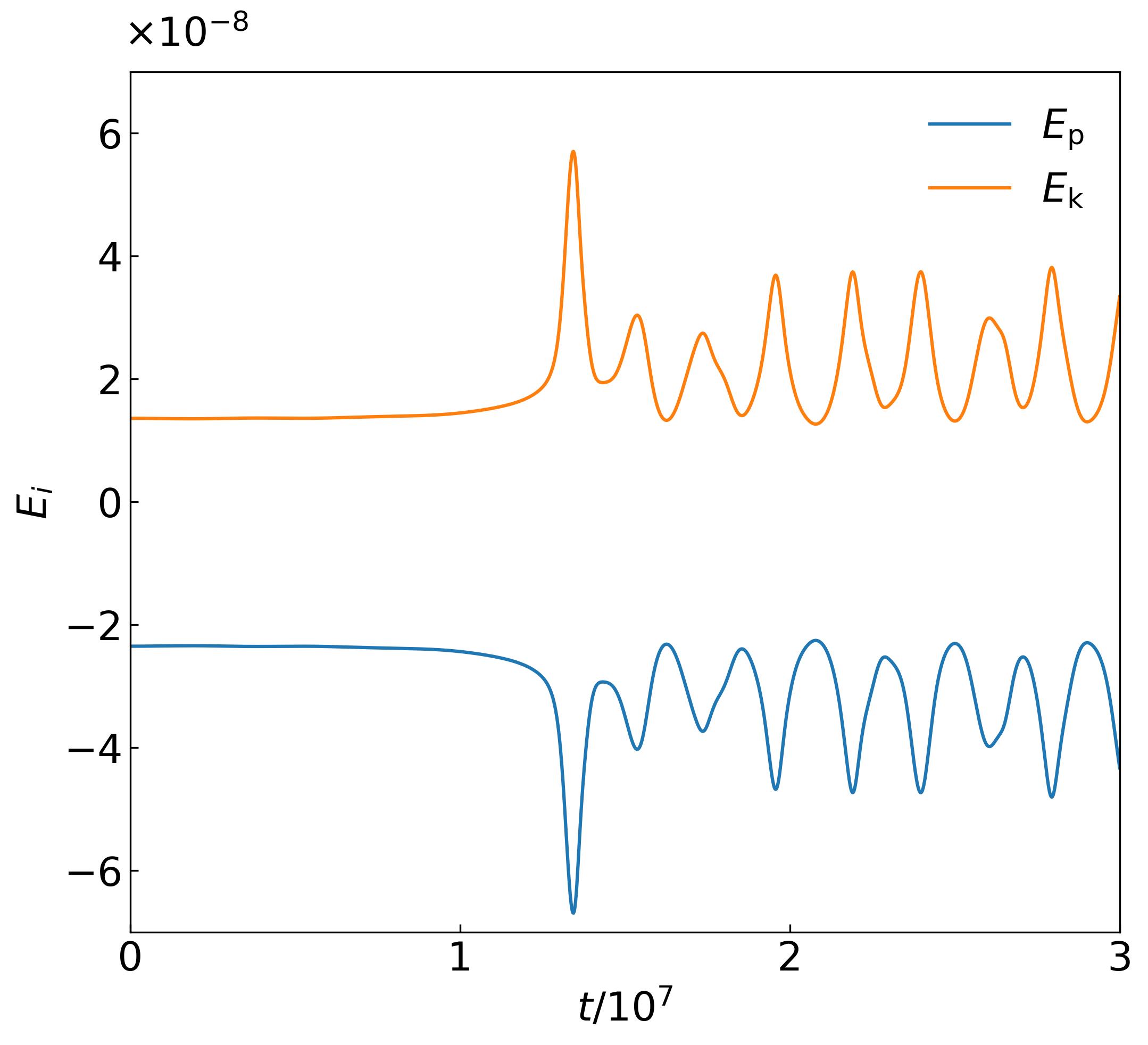
(a)

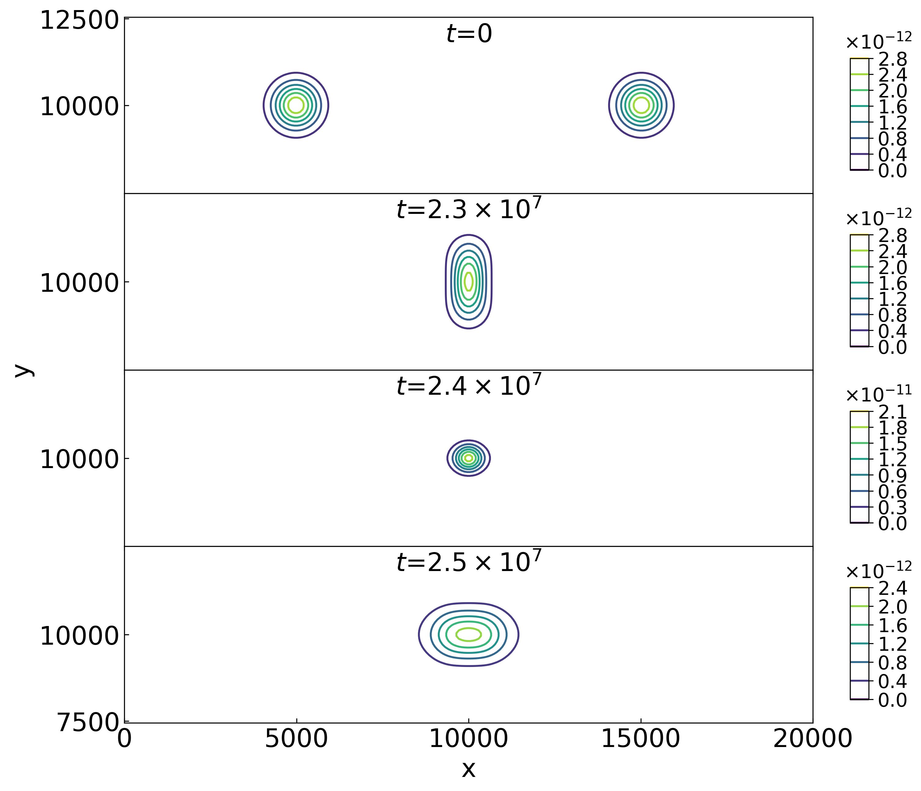
(b)

Figure 2: LEFT: Energy transfer between the kinetic energy $E_{\rm{k}}$ and the gravitational potential energy $E_{\rm{p}}$. RIGHT: Snapshots of the evolutions of FDM solitons, where the values of density contours are indicated by the side bars. For the initial configuration, the largest density of every soliton is $\lambda_{i}^{2}$ of C1 listed in Tab. 2.

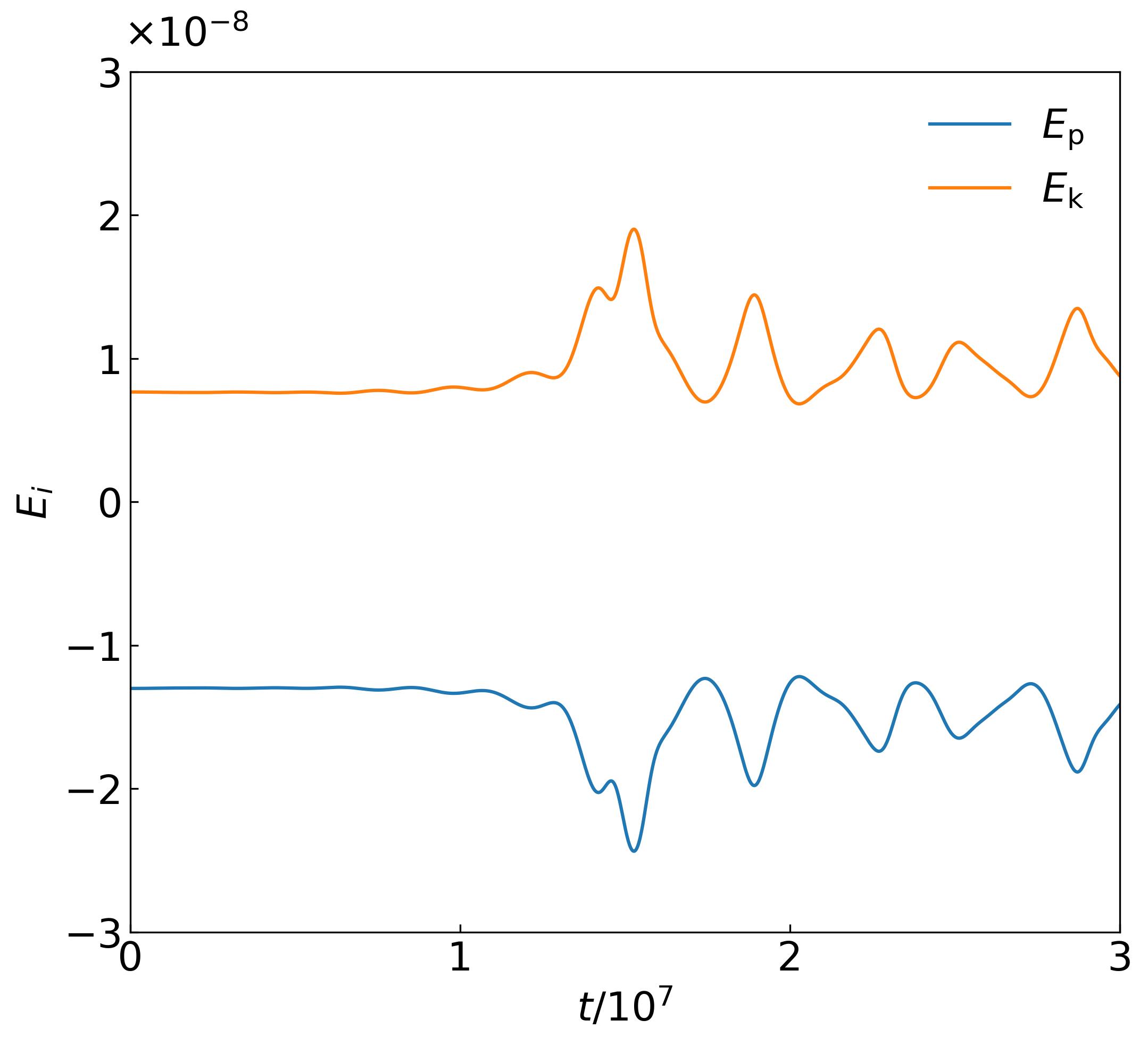
(a)

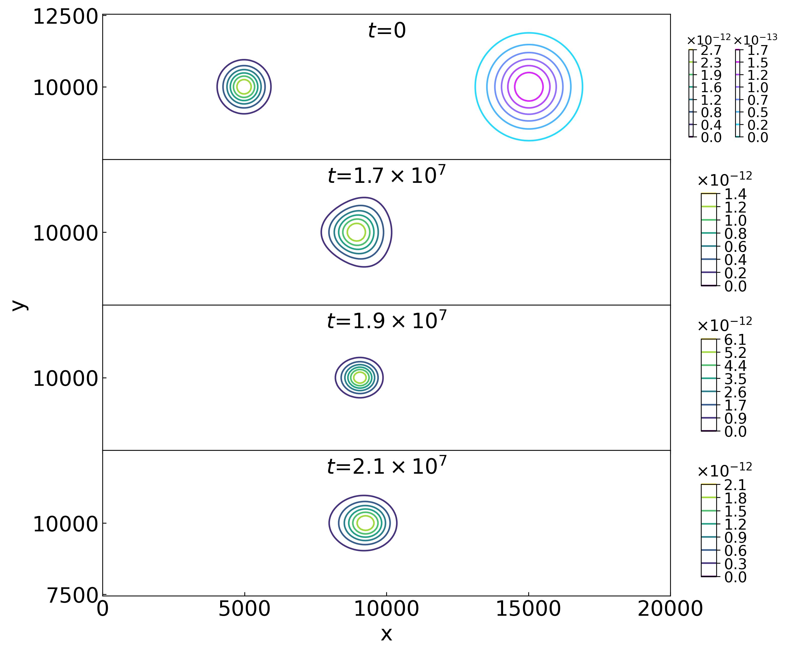
(b)

Figure 3: LEFT: Energy transfer between the kinetic energy $E_{\rm{k}}$ and the gravitational potential energy $E_{\rm{p}}$. RIGHT: Snapshots of the evolutions of FDM solitons, where the values of density contours are indicated by the side bars. For the initial configuration, the largest density of every soliton is $\lambda_{i}^{2}$ of C2 listed in Tab. 2.

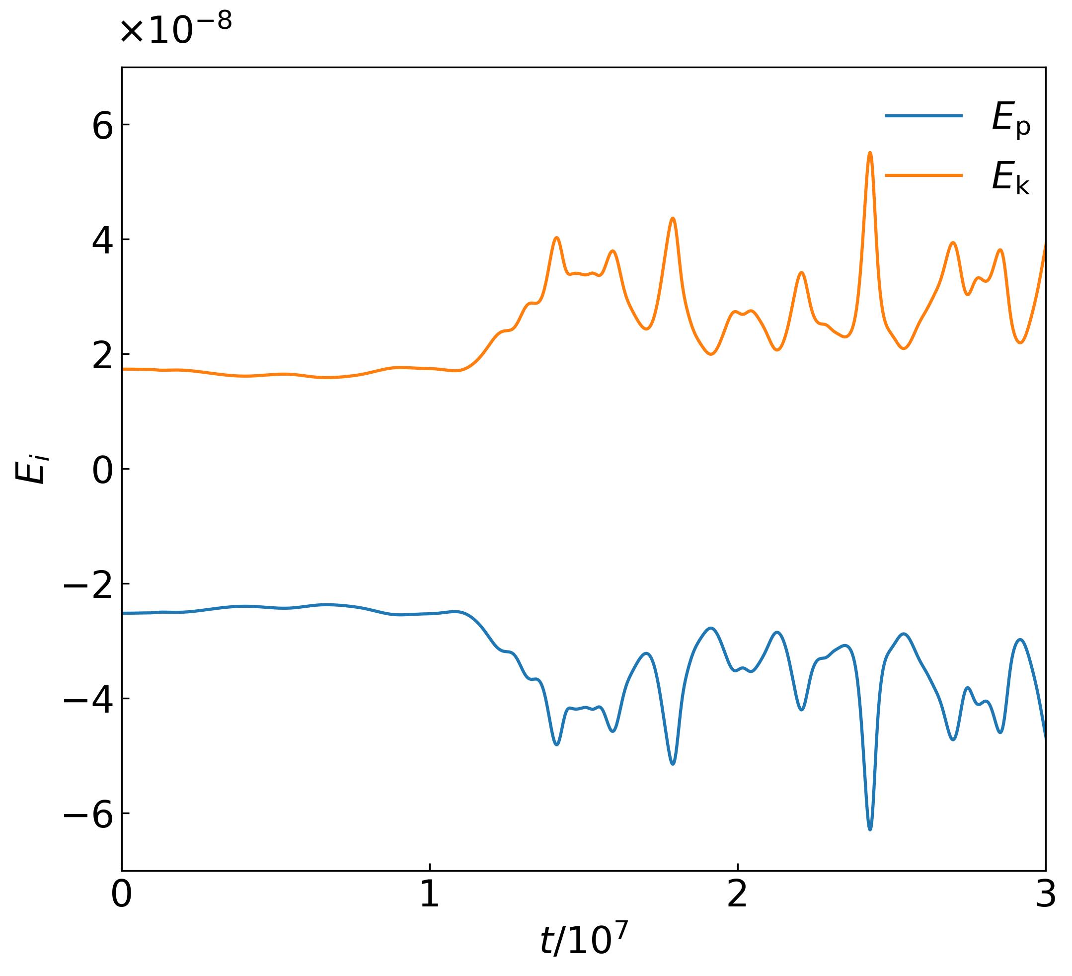
(a)

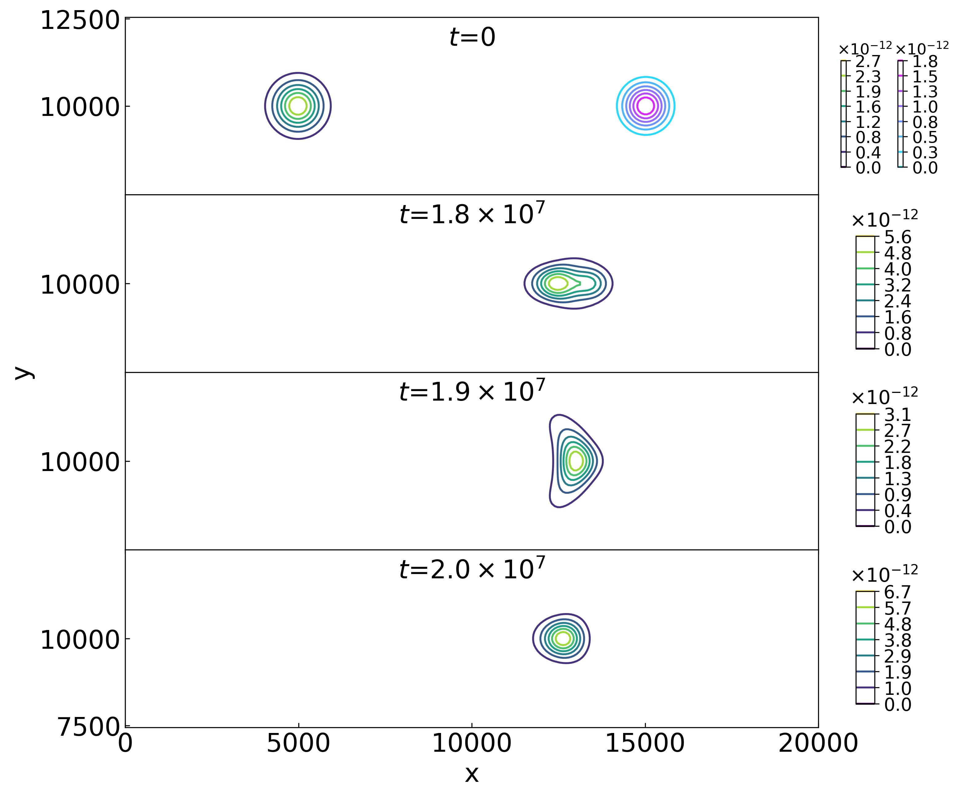
(b)

Figure 4: LEFT: Energy transfer between the kinetic energy $E_{\rm{k}}$ and the gravitational potential energy $E_{\rm{p}}$. RIGHT: Snapshots of the evolutions of FDM solitons, where the values of density contours are indicated by the side bars. For the initial configuration, the largest density of every soliton is $\lambda_{i}^{2}$ of C3 listed in Tab. 2.

IV Gravitational Waves from Post-Collision

Similarly to the GWs from head-on collisions of two Proca stars CalderonBustillo:2020fyi , GWs are also emitted from post-collisions of FDM solitons. Since the SP system itself is the weak field limit of the EKG system, we suppose that the linearized theory is valid for calculation of GWs from post-collisions of FDM solitons. Solving the wave equation for GWs (Eq. (2)) on transverse-traceless gauge, we obtain the quadrupole formula

$$h_{ij}(\vec{x},t)=\frac{2G}{c^{4}r}\frac{\mathrm{d}I^{TT}_{ij}}{\partial^{2}t}(t-r/c),$$ (15)

where $I_{ij}$ is the quadrupole moment tensor of the density of FDM soltions

$$I_{ij}=\int\rho(\vec{x},t)x_{i}x_{j}\mathrm{d}x^{3}.$$ (16)

Its counterpart on transverse-traceless gauge can be constructed with the spatial projection tensor

$$I^{TT}_{ij}=(P_{i}^{k}P_{j}^{l}-\frac{1}{2}P_{ij}P^{kl})I_{kl},$$ (17)

where $P_{ij}=\delta_{ij}-n_{i}n_{j}$ is the spatial projection tensor and $n^{\mu}=(0,0,0,1)$ is the normal vector when GWs are traveling in the $z$-direction. For explicitly, we give the two GW polarizations

$$h_{+}=\frac{2G}{c^{4}r_{0}}\frac{1}{2}\left(\frac{\partial^{2}{I}_{11}}{\partial t^{2}}(t-r_{0}/c)-\frac{\partial^{2}{I}_{22}}{\partial t^{2}}(t-r_{0}/c)\right),$$

$$h_{\times}=\frac{2G}{c^{4}r_{0}}\frac{\partial^{2}{I}_{12}}{\partial t^{2}}(t-r_{0}/c),$$ (18)

where the distance from source $r_{0}$ is set as $1$Mpc in Fig. 5, Fig. 6 and Fig. 7. Since our simulations are completely independent of the FDM mass $m$, we can rescale their amplitude and frequency by fine-tuning $m$ according to Eq. (II) and Eq. (II). For example, the GW frequency is typically (few ten-years)^-1 for $m=10^{-18}\rm{eV}/c^{2}$ or (few years)^-1 for $m=10^{-17}\rm{eV}/c^{2}$. Also, from these three figures, we find that the $h_{\times}$ polarizations are zero, which naturally results from a head-on collision in the $x$ direction, and the $h_{+}$ polarizations have a frequency higher than the frequency of energy transfer between $E_{\rm{p}}$ and $E_{\rm{k}}$, as shown in the left subplots of Fig. 2, Fig. 3 and Fig. 4.

To validate the neglect of the GW back reaction on the evolution of FDM solitons during our simulations, we integrate the energy carried away by GWs during the whole simulation and compare this integration $E_{\rm{g}}$ with the energy transfer between $E_{\rm{p}}$ and $E_{\rm{k}}$ in a period. We find that the former one is

$$E_{\rm{g}}=\frac{c^{3}r^{2}}{32\pi G}\int d\Omega\int dt\frac{\partial h_{ij}}{\partial t}\frac{\partial h^{ij}}{\partial t},$$ (19)

which is much smaller than the latter one, such as $E_{\rm{g}}/\Delta E_{\rm{p}}\approx 4\times 10^{-12}$ for C1, $E_{\rm{g}}/\Delta E_{\rm{p}}\approx 6\times 10^{-13}$ for C2 and $E_{\rm{g}}/\Delta E_{\rm{p}}\approx 2\times 10^{-12}$ for C3. Therefore, our approximation to the GW back reaction is reasonable.

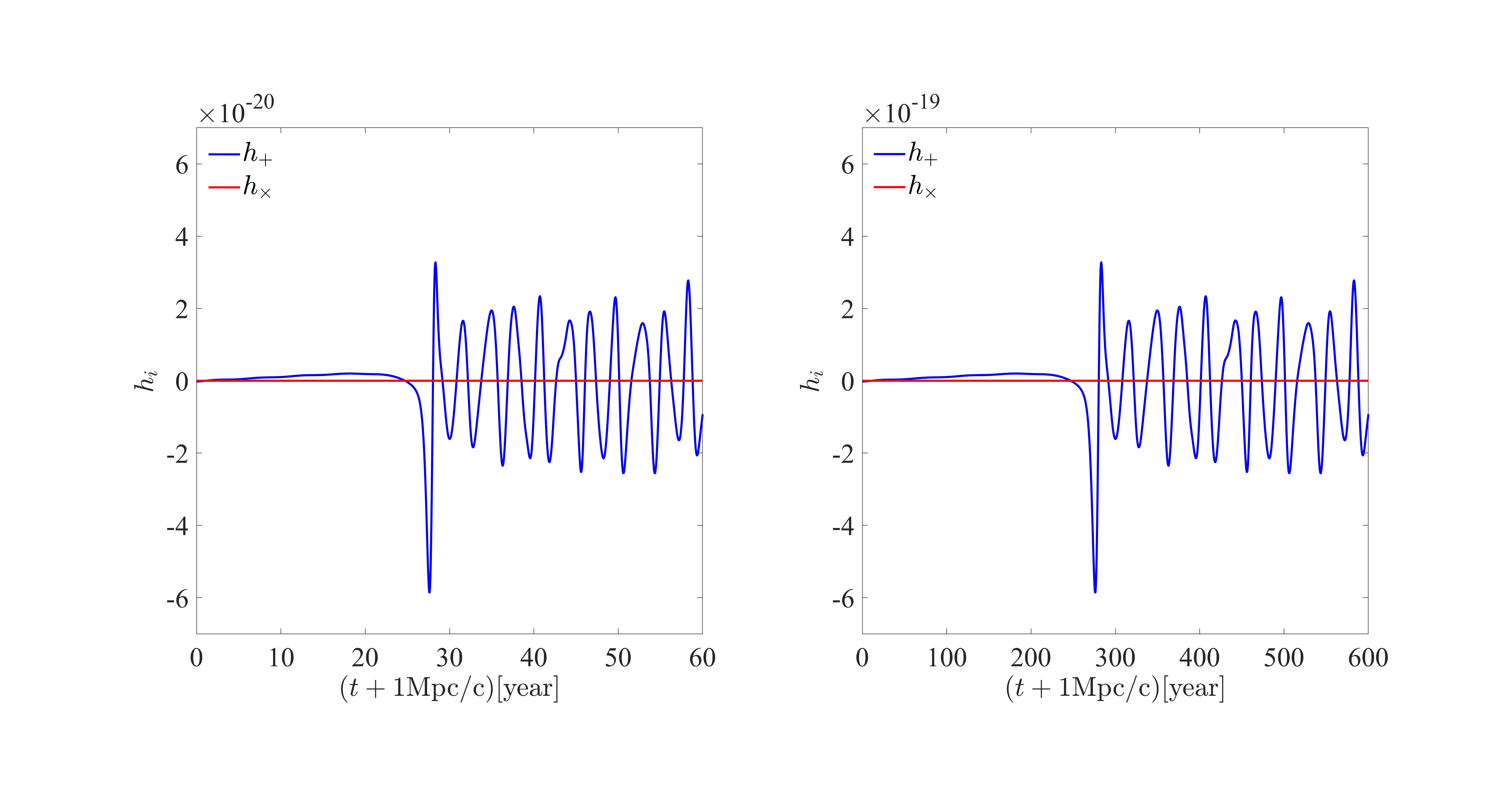
(a)

Figure 5: GWs with $h_{+}$ polarization (blue curves) and $h_{\times}$ polarization (red lines) from C1, where the distance from source is $1$Mpc and the FDM mass is $m=10^{-17}\rm{eV}/c^{2}$ (left) or $m=10^{-18}\rm{eV}/c^{2}$ (right).

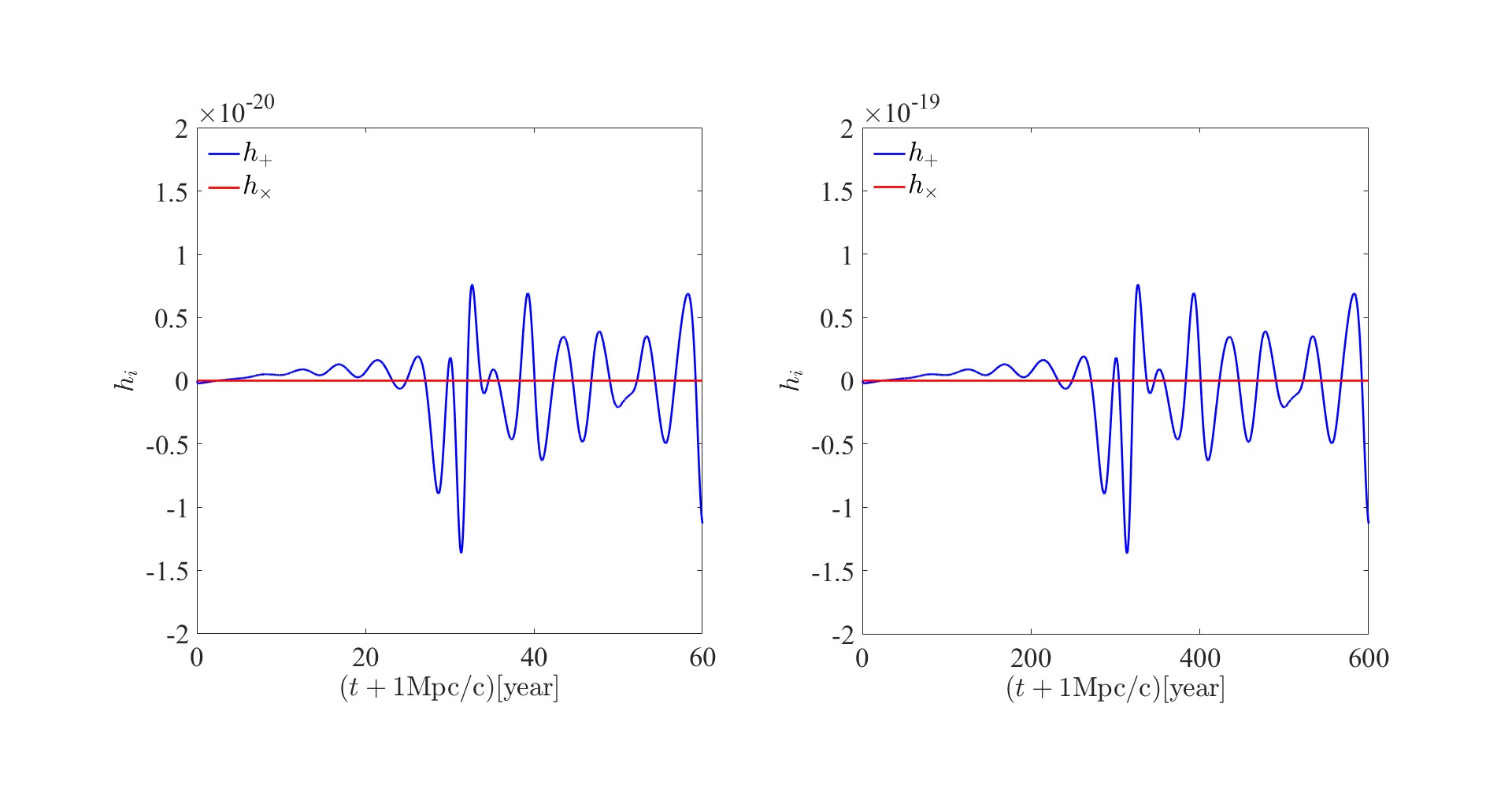
(a)

Figure 6: GWs with $h_{+}$ polarization (blue curves) and $h_{\times}$ polarization (red lines) from C2, where the distance from source is $1$Mpc and the FDM mass is $m=10^{-17}\rm{eV}/c^{2}$ (left) or $m=10^{-18}\rm{eV}/c^{2}$ (right).

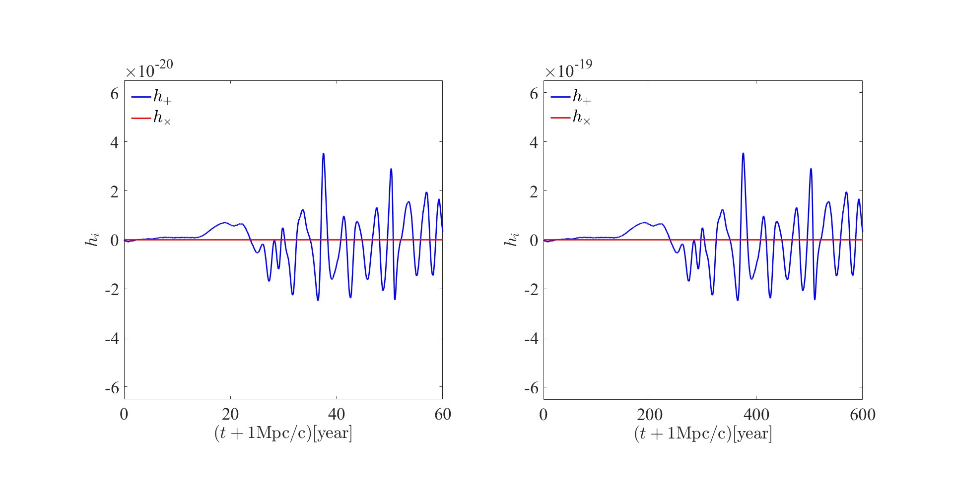
(a)

Figure 7: GWs with $h_{+}$ polarization (blue curves) and $h_{\times}$ polarization (red lines) from C3, where the distance from source is $1$Mpc and the FDM mass is $m=10^{-17}\rm{eV}/c^{2}$ (left) or $m=10^{-18}\rm{eV}/c^{2}$ (right).

V Summary and Discussion

In this paper, we propose the generation of GWs from post-collision of FDM solitons. Firstly, we turn to the shooting method to solve the SP system with spherical symmetry and build up the density profiles of the ground state and the first excited state of an isolated FDM soliton in Section II. In this section, we also propose a new adimensional unit of length, mass and time. In Section III, according to these new adimensional units, we simulate three head-on collisions: two solitons with the mass ratio equal to $1$ or $0.5$ and with the density profile as the ground state; two solitons with the mass ratio equal to $0.5$ but with the density profile as the ground state and the first excited state respectively. We find that the gravitational potential is strong enough to merge the initial two FDM solitons with each other and, during post-collisions, the energy transfer between the kinetic energy and the gravitational potential energy causes the final FDM solitons to oscillate irregularly with an adimensional frequency of $\sim 10^{-8}$. As shown in Section IV, due to this spherically asymmetric oscillation, GWs are emitted and can be easily calculated when the linearized theory is valid and the GW back reaction on the evolution of FDM solitons is ignored. By fine-tuning FDM mass $m=10^{-18}\rm{eV}/c^{2}$ or $m=10^{-17}\rm{eV}/c^{2}$, the GWs from post-collisions have a frequency of (few ten-years)^-1 or (few years)^-1respectively.

In contrast to the adimensional unit of length, mass and time applied in Paredes:2015wga ; Edwards:2018ccc ; Schive:2014hza , namely $\mathcal{L}\equiv\left(\frac{8\pi\hbar^{2}}{3m^{2}H_{0}^{2}\Omega_{m}}\right)^{1/4}\approx 121\left(\frac{10^{-23}\rm{eV}/c^{2}}{m}\right)^{1/2}\rm{kpc}$, $\mathcal{M}\equiv\frac{1}{G}\left(\frac{8\pi}{3H_{0}^{2}\Omega_{m}}\right)^{-1/4}\left(\frac{\hbar}{m}\right)^{3/2}\approx 7\times 10^{7}\left(\frac{10^{-23}\rm{eV}/c^{2}}{m}\right)^{3/2}\rm{M}_{\odot}$ and $\mathcal{T}\equiv\left(\frac{8\pi}{3H_{0}^{2}\Omega_{m}}\right)^{1/2}\approx 75.5\rm{Gyr}$, our scales (Eq. (II)) are more suitable to study the evolutions of FDM solitons in years. For example, the physical velocity $\vec{v}=\tilde{\vec{v}}\mathcal{L}\mathcal{T}^{-1}$ in this paper is independent of FDM mass $m$ and we can easily fix it as $\left(10^{-4}c,0,0\right)$. As a result, the simulations are completely independent of $m$ and the dynamics of FDM solitons can be simply rescaled by adjusting $m$. However, the dimensionless velocity $\tilde{\vec{v}}$ dose depend on $m$ in Paredes:2015wga ; Edwards:2018ccc ; Schive:2014hza if one fixes the physical velocity $\vec{v}=\tilde{\vec{v}}\mathcal{L}\mathcal{T}^{-1}$ as $\left(10^{-4}c,0,0\right)$ also. On the other hand, the dimensionless velocity $\tilde{\vec{v}}$ is an essential parameter which must be provided as one of the initial conditions. Therefore, any adjustment about $m$ will affect $\tilde{\vec{v}}$, which means that the corresponding simulation must be run again and it is not efficient enough to scan the whole parameter space and pick out the more physical systems.

The head-on collision may be not realistic enough for the evolution of FDM solitons. Usually, there should be some angular momentum for the system of FDM solitons even though it is difficult for FDM solitons to form a regular binary system because of their large size and weak self-gravitational potential sourced by their FDM density. Consequently, the presence of some angular momentum would almost equal the energy carried away by different GW polarization. For simplicity, in this paper, we confine ourselves to the GWs from post-collision of FDM solitons, whose frequency is mainly determined by the FDM soliton size and mass but not sensitive to the angular momentum of the system of FDM solitons. That is to say, we leave alone the uncertainty before collision or merger but only deal with the post-collision or ring-dwon phase. Therefore, we suppose that our results on the frequency and amplitude of GWs from post-collision of FDM solitons are also reasonable for other more general evolutions of FDM solitons.

- (1) P. A. R. Ade et al. [BICEP and Keck], “Improved Constraints on Primordial Gravitational Waves using Planck, WMAP, and BICEP/Keck Observations through the 2018 Observing Season,” Phys. Rev. Lett. 127, no.15, 151301 (2021) [arXiv:2110.00483 [astro-ph.CO]].
- (2) H. Li, S. Y. Li, Y. Liu, Y. P. Li, Y. Cai, M. Li, G. B. Zhao, C. Z. Liu, Z. W. Li and H. Xu, et al. “Probing Primordial Gravitational Waves: Ali CMB Polarization Telescope,” Natl. Sci. Rev. 6, no.1, 145-154 (2019) [arXiv:1710.03047 [astro-ph.CO]].
- (3) G. Agazie et al. [NANOGrav], “The NANOGrav 15 yr Data Set: Evidence for a Gravitational-wave Background,” Astrophys. J. Lett. 951, no.1, L8 (2023) [arXiv:2306.16213 [astro-ph.HE]].
- (4) J. Antoniadis et al. [EPTA and InPTA:], “The second data release from the European Pulsar Timing Array - III. Search for gravitational wave signals,” Astron. Astrophys. 678, A50 (2023) [arXiv:2306.16214 [astro-ph.HE]].
- (5) D. J. Reardon, A. Zic, R. M. Shannon, G. B. Hobbs, M. Bailes, V. Di Marco, A. Kapur, A. F. Rogers, E. Thrane and J. Askew, et al. “Search for an Isotropic Gravitational-wave Background with the Parkes Pulsar Timing Array,” Astrophys. J. Lett. 951, no.1, L6 (2023) [arXiv:2306.16215 [astro-ph.HE]].
- (6) P. Amaro-Seoane et al. [LISA], “Laser Interferometer Space Antenna,” [arXiv:1702.00786 [astro-ph.IM]].
- (7) W. R. Hu and Y. L. Wu, “The Taiji Program in Space for gravitational wave physics and the nature of gravity,” Natl. Sci. Rev. 4, no.5, 685-686 (2017)
- (8) J. Luo et al. [TianQin], “TianQin: a space-borne gravitational wave detector,” Class. Quant. Grav. 33, no.3, 035010 (2016) [arXiv:1512.02076 [astro-ph.IM]].
- (9) R. Abbott et al. [KAGRA, VIRGO and LIGO Scientific], “GWTC-3: Compact Binary Coalescences Observed by LIGO and Virgo during the Second Part of the Third Observing Run,” Phys. Rev. X 13, no.4, 041039 (2023) [arXiv:2111.03606 [gr-qc]].
- (10) R. Abbott et al. [LIGO Scientific and Virgo], “GWTC-2: Compact Binary Coalescences Observed by LIGO and Virgo During the First Half of the Third Observing Run,” Phys. Rev. X 11, 021053 (2021) [arXiv:2010.14527 [gr-qc]].
- (11) B. P. Abbott et al. [LIGO Scientific and Virgo], “GWTC-1: A Gravitational-Wave Transient Catalog of Compact Binary Mergers Observed by LIGO and Virgo during the First and Second Observing Runs,” Phys. Rev. X 9, no.3, 031040 (2019) [arXiv:1811.12907 [astro-ph.HE]].
- (12) S. Y. Khlebnikov and I. I. Tkachev, “Relic gravitational waves produced after preheating,” Phys. Rev. D 56, 653-660 (1997) [arXiv:hep-ph/9701423 [hep-ph]].
- (13) R. Easther and E. A. Lim, “Stochastic gravitational wave production after inflation,” JCAP 04, 010 (2006) [arXiv:astro-ph/0601617 [astro-ph]].
- (14) J. Garcia-Bellido, D. G. Figueroa and A. Sastre, “A Gravitational Wave Background from Reheating after Hybrid Inflation,” Phys. Rev. D 77, 043517 (2008) [arXiv:0707.0839 [hep-ph]].
- (15) C. Grojean and G. Servant, “Gravitational Waves from Phase Transitions at the Electroweak Scale and Beyond,” Phys. Rev. D 75, 043507 (2007) [arXiv:hep-ph/0607107 [hep-ph]].
- (16) M. Hindmarsh, S. J. Huber, K. Rummukainen and D. J. Weir, “Numerical simulations of acoustically generated gravitational waves at a first order phase transition,” Phys. Rev. D 92, no.12, 123009 (2015) [arXiv:1504.03291 [astro-ph.CO]].
- (17) M. Hindmarsh, S. J. Huber, K. Rummukainen and D. J. Weir, “Gravitational waves from the sound of a first order phase transition,” Phys. Rev. Lett. 112, 041301 (2014) [arXiv:1304.2433 [hep-ph]].
- (18) A. Kosowsky, M. S. Turner and R. Watkins, “Gravitational waves from first order cosmological phase transitions,” Phys. Rev. Lett. 69, 2026-2029 (1992)
- (19) N. Aggarwal, O. D. Aguiar, A. Bauswein, G. Cella, S. Clesse, A. M. Cruise, V. Domcke, D. G. Figueroa, A. Geraci and M. Goryachev, et al. “Challenges and opportunities of gravitational-wave searches at MHz to GHz frequencies,” Living Rev. Rel. 24, no.1, 4 (2021) [arXiv:2011.12414 [gr-qc]].
- (20) V. C. Rubin, W. K. Ford, Jr., N. Thonnard and D. Burstein, “Rotational properties of 23 SB galaxies,” Astrophys. J. 261, 439 (1982)
- (21) M. Davis, G. Efstathiou, C. S. Frenk and S. D. M. White, “The Evolution of Large Scale Structure in a Universe Dominated by Cold Dark Matter,” Astrophys. J. 292, 371-394 (1985)
- (22) D. Clowe, M. Bradac, A. H. Gonzalez, M. Markevitch, S. W. Randall, C. Jones and D. Zaritsky, “A direct empirical proof of the existence of dark matter,” Astrophys. J. Lett. 648, L109-L113 (2006) [arXiv:astro-ph/0608407 [astro-ph]].
- (23) W. Hu, R. Barkana and A. Gruzinov, “Cold and fuzzy dark matter,” Phys. Rev. Lett. 85, 1158-1161 (2000) [arXiv:astro-ph/0003365 [astro-ph]].
- (24) F. S. Guzman and L. A. Urena-Lopez, “Evolution of the Schrodinger-Newton system for a selfgravitating scalar field,” Phys. Rev. D 69, 124033 (2004) [arXiv:gr-qc/0404014 [gr-qc]].
- (25) E. Y. Davies and P. Mocz, “Fuzzy Dark Matter Soliton Cores around Supermassive Black Holes,” Mon. Not. Roy. Astron. Soc. 492, no.4, 5721-5729 (2020) [arXiv:1908.04790 [astro-ph.GA]].
- (26) A. Paredes and H. Michinel, “Interference of Dark Matter Solitons and Galactic Offsets,” Phys. Dark Univ. 12, 50-55 (2016) [arXiv:1512.05121 [astro-ph.CO]].
- (27) F. Edwards, E. Kendall, S. Hotchkiss and R. Easther, “PyUltraLight: A Pseudo-Spectral Solver for Ultralight Dark Matter Dynamics,” JCAP 10, 027 (2018) [arXiv:1807.04037 [astro-ph.CO]].
- (28) E. Munive-Villa, J. N. Lopez-Sanchez, A. A. Avilez-Lopez and F. S. Guzman, “Solving the Schrödinger-Poisson system using the coordinate adaptive moving mesh method,” Phys. Rev. D 105, no.8, 083521 (2022) [arXiv:2203.10234 [gr-qc]].
- (29) D. J. Kaup, “Klein-Gordon Geon,” Phys. Rev. 172 (1968), 1331-1342
- (30) R. Ruffini and S. Bonazzola, “Systems of self-gravitating particles in general relativity and the concept of an equation of state,” Phys. Rev. 187 (1969), 1767-1783
- (31) T. X. Ma, C. Liang, J. Yang and Y. Q. Wang, “Hybrid Proca-boson stars,” Phys. Rev. D 108, no.10, 104011 (2023) [arXiv:2304.08019 [gr-qc]].
- (32) H. Y. Schive, M. H. Liao, T. P. Woo, S. K. Wong, T. Chiueh, T. Broadhurst and W. Y. P. Hwang, “Understanding the Core-Halo Relation of Quantum Wave Dark Matter from 3D Simulations,” Phys. Rev. Lett. 113, no.26, 261302 (2014) [arXiv:1407.7762 [astro-ph.GA]].
- (33) J. Calderón Bustillo, N. Sanchis-Gual, A. Torres-Forné, J. A. Font, A. Vajpeyi, R. Smith, C. Herdeiro, E. Radu and S. H. W. Leong, “GW190521 as a Merger of Proca Stars: A Potential New Vector Boson of eV,” Phys. Rev. Lett. 126, no.8, 081101 (2021) [arXiv:2009.05376 [gr-qc]].