External Bias and Opinion Clustering in Cooperative Networks

Abstract

In this work, we consider a group of $n$ agents which interact with each other in a cooperative framework. A Laplacian-based model is proposed to govern the evolution of opinions in the group when the agents are subjected to external biases like agents’ traits, news, etc. The objective of the paper is to design a control input which leads to any desired opinion clustering even in the presence of external bias factors. Further, we also determine the conditions which ensure the reachability to any arbitrary opinion states. Note that all of these results hold for any kind of graph structure. Finally, some numerical simulations are discussed to validate these results.

, , ,

1 Introduction

Opinion dynamics in networked environments have captured the interest of diverse fields for a considerable time. It finds applications in various domains like analysis of voting patterns [1], prediction of social media trends [2], collective animal behaviours [3], etc. The focus of this paper is on opinion clustering in which more than two clusters of agents’ opinions are eventually formed in the network. Arbitrary clustering occurs in a signed network in [4] when opinions evolve by the DeGroot-based model and the subnetwork of globally reachable nodes is structurally balanced. Other extensions of DeGroot’s model in the literature include the homophily-based Hegselmann-Krause model [5], the biased assimilation model [6], the confirmation bias model [7] and scaled consensus [8] that explain opinion clustering. In these works, the clusters depends on the initial conditions and the network topology, making it difficult to reach a desired opinion cluster.

Recent works [9, 10, 11, 12, 13, 14] have addressed the opinion clustering problem towards applications such as task allocation, rendezvous problems, etc. In [9, 10, 11], the authors propose a Laplacian-based pinning control law for a network partitioned into sub-groups of agents which satisfy the in-degree balance condition. To promote opinion separation between agents in different subgroups, signed interactions are introduced between the latter; the agents within a sub-group are constrained to have strong non-negative couplings. With similar constraints, the agents form k-partite consensus in [12] in an undirected network wherein those within each sub-group cooperate, and others necessarily compete. The authors in [14] present topology-based conditions for clustering in weakly connected digraphs using Laplacian flows. The works in [10] and [11] explore the network topologies that allow desired clustering in the absence of strong interactions among agents within a subgroup. Using another approach in [13], the authors propose to partition the agents into subgroups based on graph symmetries in connected undirected networks and design a control law to drive them to the subspace of the dominant eigenvector of graph adjacency matrix for any desired opinion clustering.

In the area of opinion dynamics, along with inter-agent interactions, an agent can also be influenced by individual prejudices [15], external sources such as news and social media [16], etc. The Taylor’s model[17] is a continuous-time model that considers the evolution of opinions in the presence of agents’ biases. The effect of agent’s biases is further explored in [18], and a measure to quantify a stubborn agent’s influence depending on its position in a network is proposed. In [19], the authors propose the Friedkin-Johnsen (FJ) model which is a discrete-time analogue of the Taylor’s model. A topology-based partitioning of the network is proposed in [20] under the FJ framework along with the criteria to achieve cluster consensus under the influence of single and multiple stubborn agents. News and social media are also frequently leveraged to shape opinions in socio-political scenarios. The effect of misinformation and rumors on opinion formation is explained in [16]. In [21], the authors determine the impact of factors like news, media, and political leaders on opinion formation using a simplified Taylor’s model; the proposed approach provides an accurate estimation of the final opinions.

In contrast to the works discussed so far, the current work proposes an approach to achieve opinion clustering within a cooperative network in the presence of external bias factors. The opinion evolution is governed by a Laplacian-based model appended with a constant bias term and a control input. The bias term represents the cumulative effect of age, socio-economic conditions of the agents, social media, etc. In this work, we extend the analysis in [21] to directed networks and explore all the potential outcomes of opinion evolution in the given framework for any value of the bias term and the initial conditions. Contrary to the works in [14, 20], we present a methodology to design the control input to achieve any desired opinion clustering despite the presence of external bias. The major advantage of the work is that the analysis presented holds for any arbitrary network topology, unlike the works [9, 10, 11, 12, 13, 20, 14] which widens its scope of applicability.

The paper is organized as follows: Section 2 contains some necessary preliminaries from graph theory. Section 3 presents the model which governs the evolution of opinions. The effects of external bias factors and the conditions required to achieve any desired clustering of opinions are discussed in Sections 4 and 5, respectively. Section 6 demonstrates these results through numerical simulations. To further elaborate on the results, a realistic example has been discussed in Section 7. Finally, Section 8 concludes the paper.

2 Preliminaries

A weighted graph is represented by $\mathcal{G}=(\mathcal{V},\mathcal{E})$ where $\mathcal{V}=\{1,2,\cdots,n\}$ is the set of nodes, $\mathcal{E}\subseteq\mathcal{V}\times\mathcal{V}$ is the set of edges of the graph $\mathcal{G}$. The nodes and the edges represent the agents and their interactions in the multi-agent framework, respectively. The edge $(i,j)\ \in\mathcal{E}$ denotes an edge from node $i$ to node $j$. In an undirected graph, nodes $i$ and $j$ are neighbours if there exists an edge $(i,j)\in\mathcal{E}$. In an directed graph, for an edge $(i,j)$, the node $i$ is in-neighbor of $j$, and node $j$ is out-neighbor of node $i$. The neighbourhood of a node $i$ is $N_{i}=\{j\in\mathcal{V}$ $|$ $(i,j)\ \in\mathcal{E}\}$.

The Adjacency matrix $A\in\mathbb{R}^{n\text{x}n}$ for the graph $\mathcal{G}$ is denoted by $A=\{a_{ij}\}$. The entry $a_{ij}$ is the weight of the edge $(i,j)$. The degree of a node refers to the number of neighbours for undirected graphs. For digraphs, the notions of in-degree and out-degree exist, which refer to the number of in-neighbors and out-neighbors of a node. The out-degree matrix $D=\{d_{ij}\}$ is defined as $d_{ij}=\sum_{k\in N_{i}}a_{ik}$ for $i=j$ and $0$ otherwise. $\mathbf{1}_{n}$ and $\mathbf{0}_{n}$ denote column vectors with all entries equal to $+1$ and $0$, respectively. The matrix $I_{n}$ denotes the identity matrix of dimension $n$. The Laplacian matrix $L\in\mathbb{R}^{n\text{x}n}$ for the graph $\mathcal{G}$ is defined as

$$L=D-A.$$ (1)

It follows from eqn. (1), that $L\mathbf{1}_{n}=\mathbf{0}_{n}$ therefore, Laplacian matrix $L$ will always have a zero eigenvalue in a cooperative framework. The non-zero eigenvalues of the Laplacian matrix have a strictly positive real part.

Next, we discuss some graph properties. A sink is a node with a zero out-degree. A node that is reachable from every other node is called a globally reachable node. If every node is reachable from every other node, the graph is strongly connected. A weakly connected graph is a directed graph that is not strongly connected, but its undirected version is connected. A condensation graph $C(\mathcal{G})$ of a digraph $\mathcal{G}$ has nodes consisting of strongly connected components of the graph $\mathcal{G}$. There exists an edge from node $I$ to node $J$ in $C(\mathcal{G})$, if and only if there exists an edge from a node in $I$ to a node in $J$ in graph $\mathcal{G}$ where $I$ and $J$ denote the strongly connected components of graph $\mathcal{G}$ in $C(\mathcal{G})$.

3 Opinion Modelling

In this work, we study the evolution of opinions in a group of $n$ agents interacting in a cooperative social framework. The evolution of opinions, in general, depends on various factors which are broadly classified as endogenous and exogenous [22]. The endogenous factors arise from the interpersonal relationship between the agents. The exogenous factors are external to the group and depend on social factors like gender, age, socio-economic conditions, and media. We categorize the exogenous factors into two types: (a) those which are pre-existing and cannot be modified or controlled, viz., age and gender, denoted as a bias term $\mathbf{b}$ (b) those which can be controlled, viz., news and advertisements, denoted as a control input $\mathbf{u}$. Along with interpersonal relations, the opinions of the agents are also affected by these exogenous factors, given cumulatively by $\mathbf{b}+\mathbf{u}$. We treat $\mathbf{u}$ as the control input, which is used to achieve the desired opinion patterns like consensus, polarisation, and clustering.

Example [23]: During the COVID-19 pandemic, the population of the US was polarised into pro-vaccine and anti-vaccine groups due to the influence of their existing beliefs, misinformation spread by social media interactions and bots, etc. All of these are categorised as a bias term b. The Government and health organisations used advisories and fact checks to counter the misinformation on social media. Further, they encouraged well-known figures from various fields to get immunised and raise awareness among people. These targeted interventions can be categorised under control input u.

Considering the presence of both endogenous and exogenous factors, in this work, we propose the following continuous time opinion model for the $i^{th}$ agent,

$$\dot{x}_{i}=\sum_{j\in N_{i}}a_{ij}(x_{j}(t)-x_{i}(t))+b_{i}+u_{i}$$ (2)

where $x_{i}$, $b_{i}$, and $u_{i}$ represent the opinion, the bias term, and the control input of the $i^{th}$ agent, respectively. In eqn. (2), the term $a_{ij}$ represents agent $j$’s influence on agent $i$. In vector form, the opinion dynamics given in eqn. (2) can be re-written as,

$$\dot{x}=-Lx+\mathbf{b}+\mathbf{u}$$ (3)

where $L$ is the Laplacian matrix for the underlying graph $\mathcal{G}$ as defined in eqn. (1), $\mathbf{b}=(b_{1},b_{2},\cdots,b_{n})^{T}$ is the constant bias vector and $\mathbf{u}=(u_{1},u_{2},\cdots,u_{n})^{T}$ is the control input vector. This model is used to reflect the effect of the societal bias factors $b_{i}$ on the evolution of opinions. In real world scenarios like bimodal coalitions, duo-polistic markets, and competing international alliances, polarisation can be extremely undesirable. Hence, we further aim to design $u_{i}$ so as to mitigate the undesired effects of $b_{i}$ through the desired collective behaviour of clustering.

4 The effect of bias on opinion formation

In this section, we study the effect of pre-existing exogenous bias factors on opinion formation in the absence of any control input $\mathbf{u}$. Without the bias vector $\mathbf{b}$, the opinion model given in eqn. (2) becomes the well-studied Laplacian flow [24] which leads to consensus for several graph structures; the additional term b can sway opinion states away from consensus.

To study the evolution of the opinion states with time, we rewrite $-L$ using its canonical decomposition as $-L=VJW^{T}$ where $V$ and $W$ are the matrices consisting of the right eigenvectors $\mathbf{v}_{i}$ and the left eigenvectors $\mathbf{w}_{i}$ of $-L$, respectively, along their columns for $i\in\{1,...,n\}$. The matrix $J$ is the block diagonal Jordan normal form (see Section 2.1.2 in [24]).

The spectrum of $-L$ is denoted by $\sigma=\{\sigma_{1},\sigma_{2},\cdots,\sigma_{n}\}$. Without loss of generality, the initial time $t_{0}$ is assumed to be $0$ throughout the paper. Then, the solution of eqn. (3) with $\mathbf{u}=\mathbf{0}_{n}$ [25] can be written as,

$$x(t)=Ve^{Jt}W^{T}x_{0}+V\int_{0}^{t}e^{J(t-\tau)}d\tau W^{T}\mathbf{b}.$$ (4)

The subsequent result aids our understanding of how biases affect opinion formation, with a discussion on the stability aspects of the arising collective behaviours.

Theorem 1.

The system (3) with $\mathbf{u}=\mathbf{0}_{n}$ admits a stable solution regardless of the connectivity of the graph, if and only if the following equation holds

$$\mathbf{w}_{i}^{T}\mathbf{b}=0\ \forall\sigma_{i}=0$$ (5)

where $i\in\{1,2,\cdots,n\}.$ Otherwise, it is unstable. Let $n_{z}$ be the number of zero eigenvalues of $-L$, then for the stable case, at steady state $\lim_{t\to\infty}x(t)$ can be given as,

$$\bar{x}=V\left[\mathbf{w}_{1}^{T}x_{0},\cdots,\mathbf{w}_{n_{z}}^{T}x_{0},\left[-(\tilde{J}^{-1})\tilde{W}^{T}\mathbf{b}\right]^{T}\right]^{T}$$ (6)

where $\tilde{J}$ and $\tilde{W}$ are submatrices of $J$ and $W$, respectively, pertaining to the non-zero eigenvalues of $-L$. For the unstable case, the weighted average of the opinion states evolves with time, as given below,

$$\mathbf{w}_{i}^{T}x(t)=\mathbf{w}_{i}^{T}(x_{0}+\mathbf{b}t)\qquad\forall\sigma_{i}=0,t\geq 0.$$ (7)

Proof.

We start the proof by showing that eqn. (5) is necessary for convergence irrespective of network connectivity. It is known that the Jordan blocks of the Laplacian matrix with zero eigenvalues are of size $1$, and the multiplicity of zero eigenvalues depends on the connectivity of the graph [24].

We decompose $J$ into two parts, one with only zero eigenvalues and the other with non-zero values $\tilde{J}$, which is invertible. Hence, we can rewrite eqn. (4) as,

$$x(t)=Ve^{Jt}W^{T}x_{0}+V\begin{bmatrix}C&0\\ 0&(e^{\tilde{J}t}-I)\tilde{J}^{-1}\end{bmatrix}W^{T}\mathbf{b}$$ (8)

where $C=diag(t,t,\cdots,t)$ is a diagonal matrix with the time-varying terms occurring due to the integration of the part of $J$ corresponding to the zero eigenvalues, the matrix $C$ is a square matrix with dimension $n_{z}$.

$$\lim_{t\to\infty}x(t)=\sum_{i=1}^{n_{z}}\mathbf{v}_{i}\mathbf{w}_{i}^{T}x_{0}+ \lim_{t\to\infty}V\Big{[}\mathbf{w}_{1}^{T}\mathbf{b}t,\cdots,\mathbf{w}_{n_{z}}^{T}\mathbf{b}t,$$

$$\big{[}(e^{\tilde{J}t}-I)\tilde{J}^{-1}\tilde{W}^{T}\mathbf{b}\big{]}^{T}\Big{]}^{T}.$$

The solution $x(t)$ becomes stable when the time-varying terms do not exist. By applying eqn. (5), the time-varying terms vanish such that

$$\bar{x}=\sum_{i=1}^{n_{z}}\mathbf{v}_{i}\mathbf{w}_{i}^{T}x_{0}+V\left[0,\cdots,0,\left[-\tilde{J}^{-1}\tilde{W}^{T}\mathbf{b}\right]^{T}\right]^{T}$$

Further rearrangement results in a stable solution as given by eqn. (6).

Next, we consider the case when eqn. (3) admits a stable solution. At steady state, we have $\dot{x}=0$ which implies $-L\bar{x}+\mathbf{b}=0$. Rearranging and premultiplying it with $\mathbf{w}_{i}^{T}$, we get $\mathbf{w}_{i}^{T}\mathbf{b}=\mathbf{w}_{i}^{T}L\bar{x}$. Note that $\mathbf{w}_{i}^{T}L=\mathbf{0}_{n}^{T}\ \forall\ \sigma_{i}=0$ as since $\mathbf{w}_{i}$ is the left eigenvector corresponding to the $\sigma_{i}=0$. This implies $\mathbf{w}_{i}^{T}\mathbf{b}=0$ for every zero-eigenvalue. This concludes the discussion on the stability of system (3).

In the case when system (3) is unstable, $\mathbf{w}^{T}_{i}\mathbf{b}\neq 0$. Then, $x(t)$ can be obtained by simplifying eqn. (8) as,

$$x(t)=V\bigg{[}\mathbf{w}_{1}^{T}(x_{0}+\mathbf{b}t),\cdots,\mathbf{w}_{n_{z}}^{T}(x_{0}+\mathbf{b}t),\left[-(\tilde{J}^{-1})\tilde{W}^{T}\mathbf{b}\right]^{T}\bigg{]}^{T}$$ (9)

The eigenvectors of $L$ are normalized to satisfy $W^{T}V=I_{n}$. Hence, the terms with $\mathbf{v}_{j\neq i}$, $j\in\{1,2,\cdots,n\}$, disappear resulting in eqn. (7). Hence, proved. ∎

The stable solution given in eqn. (6) simply means that the opinion states converge to finite values. Theorem 1 shows that such a behaviour can be achieved irrespective of the graph connectivity. The steady state solution given in eqn. (6) can be refined further for some specific graph structures whose Laplacian matrices have zero as a simple eigenvalue.

Corollary 1.

For a connected undirected graph, system (3) admits a stable solution if and only if $\sum_{i=0}^{n}b_{i}=0$. At steady state, eqn. (6) becomes,

$$\bar{x}=V\left[\sum_{i=1}^{n}\frac{x_{0i}}{n},\frac{-\mathbf{w}_{2}^{T}\mathbf{b}}{\sigma_{2}},\frac{-\mathbf{w}_{3}^{T}\mathbf{b}}{\sigma_{3}},\cdots,\frac{-\mathbf{w}_{n}^{T}\mathbf{b}}{\sigma_{n}}\right]^{T}$$ (10)

For $\sum_{i=1}^{n}b_{i}\neq 0$ system (3) is unstable, and the average value of the opinion states evolves with time as given below,

$$\frac{1}{n}\sum_{i=1}^{n}x_{i}(t)=\frac{1}{n}\sum_{i=1}^{n}x_{0i}+\frac{t}{n}\sum_{i=1}^{n}b_{i}\ \ \ t\geq 0$$ (11)

Proof.

It is already known that for a connected undirected graph, the Laplacian matrix is symmetric and has a simple $0$ eigenvalue. The corresponding right and left eigenvectors are $\mathbf{1}_{n}$ and $\mathbf{1}_{n}/n$, chosen to satisfy $\mathbf{v}_{1}^{T}\mathbf{w}_{1}=1$. Then, eqn. (5) simplifies to $\sum_{i=0}^{n}b_{i}=0$ and eqn. (7) to eqn. (11). Since the inverse of the $i^{th}$ Jordan block $J_{i}^{-1}=\frac{1}{\sigma_{i}}$ for all $\sigma_{i}\neq 0$, eqn. (6) reduces to eqn. (10). Hence, proved. ∎

Corollary 2.

For a digraph containing a globally reachable node(s), system (3) admits a stable solution if and only if

$$\sum_{i\in N_{G}}\mathbf{w}_{1i}b_{i}=0.$$ (12)

At steady state, eqn. (6) becomes,

$$\bar{x}=V\left[\mathbf{w}_{1}^{T}x_{0},\left[-(\tilde{J}^{-1})\tilde{W}^{T}\mathbf{b}\right]^{T}\right]^{T}$$ (13)

where $\mathbf{w}_{1}=[w_{11},w_{12}is,\cdots,w_{1n}]^{T}$ is the left eigenvector and $N_{G}$ is the set of globally reachable node(s). For $\mathbf{w}_{1}^{T}\mathbf{b}\neq 0$, system (3) becomes unstable, and the weighted average of the opinion states evolves with time as

$$\mathbf{w}_{1}^{T}x(t)=\mathbf{w}_{1}^{T}x_{0}+\mathbf{w}_{1}^{T}\mathbf{b}t$$ (14)

Proof.

We know that $L$ has a simple zero-eigenvalue (see Theorem $6.6$ in [24]). The right eigenvector is $\mathbf{1}_{n}$ and, for the left eigenvector, $\mathbf{w}_{1i}>0$ $\forall$ $i\in N_{G}$ and is zero otherwise. Using these results, the rest of the proof follows in the same manner as that of Corollary 1. ∎

Note that strongly connected digraphs form a special case of the graphs discussed in Corollary 2 with $N_{G}=\{1,2,\cdots,n\}$. So far, we have discussed the conditions on the external bias factors $\mathbf{b}$ in Theorem 1, which are required for stability. However, $\mathbf{b}$ may not even satisfy it. Even if it does, the stable opinion states of the group could become undesirable (e.g. polarisation). In the next section, we present the conditions which guarantee the arbitrary clustering of opinion states while maintaining stability.

5 Clustering of opinion states

In this section, we design the control input $\mathbf{u}$ to drive the opinion states of system (3) to desired opinion clusters in the presence of a constant bias vector $\mathbf{b}$. We begin by exploring the conditions required for the stability of the system. Replacing $\mathbf{b}$ with $\mathbf{(b+u)}$ in the Theorem 1 results in the stability condition given as $\mathbf{w}_{i}^{T}(\mathbf{b}+\mathbf{u})=0\ \forall\ \sigma_{i}=0$. Furthermore,

$$\mathbf{w}_{i}^{T}x(t)=\mathbf{w}_{i}^{T}x(0)\qquad\forall\sigma_{i}=0,t\geq 0$$ (15)

where $i\in\{1,2,\cdots,n\}.$

Now, we discuss two specific classes of graphs that have zero as simple eigenvalues.

• For a connected undirected graph, it follows that $\sum_{i=1}^{n}(b_{i}+u_{i})=0$ for stability. Then, $\sum_{i=1}^{n}x_{i}(t)=\sum_{i=1}^{n}x_{i}(0)\ t\geq 0$.

• For a digraph containing a globally reachable node, $\mathbf{w}_{1}^{T}(\mathbf{b}+\mathbf{u})=0$ must hold for stability. In this case, $\mathbf{w}_{1}^{T}x(t)=\mathbf{w}_{1}^{T}x(0)\ t\geq 0$.

It is possible to stabilize the system using eqn.(15). However, it is not yet clear if we could achieve the desired opinion state as stable behaviour or not. Now, we try to address this issue starting with the following discussion.

Remark 1.

Using eqn. (15) the reachable set of opinion states is defined as

$$X_{R}\vcentcolon=\{x_{d}\in\mathbb{R}^{n}|\mathbf{w}_{i}^{T}x_{d}=\mathbf{w}_{i}^{T}x_{0}\ \forall\ \sigma_{i}=0\}$$ (16)

where $i\in\{1,2,\cdots,n\}$. If the stable desired opinion states $x_{d}$ belongs to the reachable set $X_{R}$, then $\dot{x}=0$ at steady state. This gives $-Lx_{d}+(\mathbf{b}+\mathbf{u})=0$. Then, the control input $\mathbf{u}$ to reach an opinion state $x_{d}$ is given by

$$\mathbf{u}=Lx_{d}-\mathbf{b}.$$ (17)

Remark 1 shows that it is not possible to achieve $x\in\mathbb{R}^{n}$\$X_{R}$ using eqn. (2). The following result allows us to make the entire $\mathbb{R}^{n}$ space reachable.

Theorem 2.

For a given initial state $x_{0}$ and a constant bias vector $\mathbf{b}$, system (3) admits any stable desired opinion state $x_{d}$, irrespective of the connectivity of the graph by designing the control input $\mathbf{u}$ as given below,

1. if $\mathbf{w}_{i}^{T}x_{d}=\mathbf{w}_{i}^{T}x_{0}$, then $\mathbf{u}$ is given by eqn. (17),

2. else, $\mathbf{u}$ satisfies the condition,

   $$\mathbf{w}_{i}^{T}(\mathbf{b}+\mathbf{u})=(\mathbf{w}_{i}^{T}x_{d}-\mathbf{w}_{i}^{T}x_{0})/\bar{t},~~\forall\sigma_{i}=0$$ (18)

   for $t\leqslant\bar{t}$ and is given by eqn. (17) for $t>\bar{t}$ where $\bar{t}$ is chosen arbitrarily in $(0,\infty)$ and $i\in\{1,2,\cdots,n\}$.

Proof.

When the desired opinion state $x_{d}$ lies in the reachable set $X_{R}$, then $\mathbf{u}$ can be calculated using Remark 1, which leads to condition $(a)$ of the theorem.

When $x_{d}\not\in X_{R}$, it is not possible to reach $x_{d}$ using the control input given in eqn. (17). To alleviate this issue, we propose a two-stage solution: first, we reach some $\tilde{x}\neq\{x_{0},x_{d}\}$ from where $x_{d}$ is reachable; thereafter, we use eqn. (17) to calculate the suitable control input which is required to reach $x_{d}$.

Note that it is not possible to reach $\tilde{x}$ starting from $x_{0}$ through a stable system behaviour as $\mathbf{w}_{i}^{T}\tilde{x}\neq\mathbf{w}_{i}^{T}x_{0}$. In the presence of $\mathbf{b}$ and $\mathbf{u}$, an unstable behaviour can be modelled using eqn. (7) as,

$$\mathbf{w}_{i}^{T}x(t)=\mathbf{w}_{i}^{T}(x_{0}+\mathbf{(b+u)}t)$$ (19)

for $t\leqslant\bar{t}$, where $\bar{t}\in(0,\infty)$ is the time till which the unstable behaviour exists such that $\tilde{x}=x(\bar{t})$.

In the second stage, $\mathbf{w}_{i}^{T}x_{d}=\mathbf{w}_{i}^{T}x(\bar{t})$ holds as $x_{d}$ is reachable from $x(\bar{t})$. Then, at $t=\bar{t}$, eqn. (19) becomes $\mathbf{w}_{i}^{T}x_{d}=\mathbf{w}_{i}^{T}(x_{0}+\mathbf{(b+u)}\bar{t}$. Re-arranging this equation gives eqn. (18) which is the necessary condition the control input $\mathbf{u}$ must satisfy. For $t>\bar{t}$, using eqn. (17) results in the desired behaviour as discussed in Remark 1. Hence, proved. ∎

Using the results discussed in Theorem 2, it is possible to obtain any desired opinion clusters which lie in $\mathbb{R}^{n}$. Clustering of opinions is often a desired outcome as it prevents polarisation. In the next section, we discuss some simulations to illustrate these results.

6 Simulation Results

Figure 1: Graph topology

In this section, numerical simulations are presented to validate the theoretical results discussed in the paper. We consider the graph shown in Fig. 1. The initial opinion states are $x(0)=\left[-6,4,-5,5,2,0\right]^{T}$. Let the external bias factors be such that $\mathbf{b}=\left[-20,20,20,-20,20,-20\right]^{T}$. We know from Theorem 1 that system (3) admits a stable solution if $\mathbf{b}$ satisfies eqn. (5) and $\mathbf{u}=\mathbf{0}_{n}$. The same can be validated by the evolution of the opinion states shown in Fig. 2. At steady state, $\bar{x}=\left[-10,10,10,-10,10,-10\right]^{T}$ which agrees with eqn. (6). As we can clearly see in Fig. 2, the bias $\mathbf{b}$ is causing polarisation in the group of agents.

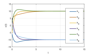
Figure 2: Polarisation of opinion states

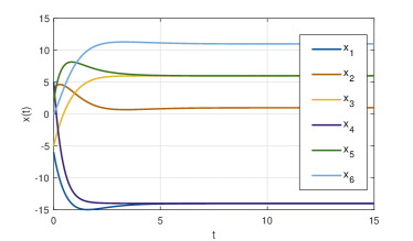
Figure 3: Clustering of opinion states

In this case, an appropriate control input to counter the effect of the bias $\mathbf{b}$ can be designed by using Remark 1 as $\mathbf{u}=\left[0,-5,-2,-20,0,25\right]^{T}$. Then, system (3) results in the clustering of opinions as shown in Fig. 3 where final opinion states are $x_{f}=[-14,1,6,-14,6,11]^{T}$. Similarly, any desired opinion pattern can be achieved in an arbitrary graph structure.

7 Discussion

In the US 2016 Presidential election, it has been shown that social media and fake news had a significant role to play in the outcome of the election [26]. In the previous elections due to the absence of such large-scale misinformation campaigns, the individuals were not as polarised. Therefore, it is evident that social media can foster polarising behaviours by using biasing factors as shown in Fig. 2. By designing the control input using Theorem 2, opinion clustering is achieved as shown in Fig. 3. Thus, the adverse effects of bias can be reduced by designing a suitable control input.

8 Conclusion

In this paper, we study the effect of external bias factors on the evolution of opinions in a cooperative network with any arbitrary connectivity. We segregate the external factors into a bias term $\mathbf{b}$ like age, gender, etc. which we cannot control or modify, and a control input $\mathbf{u}$ like advertisement, news, etc. which we can control. In the presence of a constant external bias $\mathbf{b}$, we provide the conditions which ensure the stability of the final opinion states of the agents. These conditions guarantee the convergence of the opinion states only to a finite set of values at a steady state. In the proposed framework, we further show that it is possible to design the control input $\mathbf{u}$ to extend the reachable set of opinion states to $\mathbb{R}^{n}$. By designing an appropriate control input, the undesirable effects of external bias factors like polarisation can be negated. Furthermore, any desired opinion pattern like consensus, polarisation, and clustering of opinions can also be achieved. In future, we plan to develop a nonlinear model in the given framework to better emulate a real world scenario.

References

- [1] Victor S Dotsenko, Carlos Mejía-Monasterio, and Gleb Oshanin. Negative response to an excessive bias by a mixed population of voters. arXiv preprint arXiv:1703.10404, 2017.
- [2] Yuriy Gorodnichenko, Tho Pham, and Oleksandr Talavera. Social media, sentiment and public opinions: Evidence from# brexit and# uselection. European Economic Review, 136:103772, 2021.
- [3] Vaibhav Srivastava and Naomi Ehrich Leonard. Bio-inspired decision-making and control: From honeybees and neurons to network design. In 2017 American Control Conference (ACC), pages 2026–2039. IEEE, 2017.
- [4] Weiguo Xia, Ming Cao, and Karl Henrik Johansson. Structural balance and opinion separation in trust–mistrust social networks. IEEE Transactions on Control of Network Systems, 3(1):46–56, 2016.
- [5] Hegselmann Rainer and Ulrich Krause. Opinion dynamics and bounded confidence: Models, analysis and simulation. Journal of Artificial Societies and Social Simulation, 5(3), 2002.
- [6] Pranav Dandekar, Ashish Goel, and David T. Lee. Biased assimilation, homophily, and the dynamics of polarization. Proceedings of the National Academy of Sciences, 110(15):5791–5796, 2013.
- [7] Yanbing Mao, Sadegh Bolouki, and Emrah Akyol. On the evolution of public opinion in the presence of confirmation bias. In 2018 IEEE Conference on Decision and Control (CDC), pages 5352–5357, 2018.
- [8] Sandip Roy. Scaled consensus. Automatica, 51:259–262, 2015.
- [9] Weiguo Xia and Ming Cao. Clustering in diffusively coupled networks. Automatica, 47(11):2395–2405, 2011.
- [10] Jiahu Qin and Changbin Yu. Cluster consensus control of generic linear multi-agent systems under directed topology with acyclic partition. Automatica, 49(9):2898–2905, 2013.
- [11] Shengping Luo and Dan Ye. Cluster consensus control of linear multiagent systems under directed topology with general partition. IEEE Transactions on Automatic Control, 67(4):1929–1936, 2022.
- [12] Giulia De Pasquale and Maria Elena Valcher. Consensus for clusters of agents with cooperative and antagonistic relationships. Automatica, 135:110002, 2022.
- [13] Cinzia Tomaselli, Lucia Valentina Gambuzza, Francesco Sorrentino, and Mattia Frasca. Multiconsensus induced by network symmetries. Systems & Control Letters, 181:105629, 2023.
- [14] Jeong-Min Ma, Hyung-Gon Lee, Hyo-Sung Ahn, Kevin L Moore, and Kwang-Kyo Oh. Topological approach and analysis of clustering in consensus networks. Systems & Control Letters, 183:105699, 2024.
- [15] Vineeth S Varma, Irinel-Constantin Morărescu, and Mehdi Ayouni. Analysis of opinion dynamics under binary exogenous and endogenous signals. Nonlinear Analysis: Hybrid Systems, 38:100910, 2020.
- [16] Michela Del Vicario, Alessandro Bessi, Fabiana Zollo, Fabio Petroni, Antonio Scala, Guido Caldarelli, H. Eugene Stanley, and Walter Quattrociocchi. The spreading of misinformation online. Proceedings of the National Academy of Sciences, 113(3):554–559, 2016.
- [17] Michael Taylor. Towards a mathematical theory of influence and attitude change. Human Relations, 21(2):121–139, 1968.
- [18] Fabian Baumann, Igor M Sokolov, and Melvyn Tyloo. A laplacian approach to stubborn agents and their role in opinion formation on influence networks. Physica A: Statistical Mechanics and its Applications, 557:124869, 2020.
- [19] Noah E Friedkin and Eugene C Johnsen. Social influence and opinions. Journal of Mathematical Sociology, 15(3-4):193–206, 1990.
- [20] Lingling Yao, Dongmei Xie, and Jianlei Zhang. Cluster consensus of opinion dynamics with stubborn individuals. Systems & Control Letters, 165:105267, 2022.
- [21] Giuseppe Fedele, Enrico Bozzo, and Luigi D’Alfonso. On the impact of agents with influenced opinions in the swarm social behavior. IEEE Control Systems Letters, 7:2317–2322, 2023.
- [22] Noah E. Friedkin and Eugene C. Johnsen. Social positions in influence networks. Social Networks, 19(3):209–222, 1997.
- [23] Edward Alan Glasper. Reducing the impact of anti-vaccine propaganda on family health, 2021.
- [24] F. Bullo. Lectures on Network Systems. Kindle Direct Publishing, 1.6 edition, 2022.
- [25] Chi-Tsong Chen. Linear system theory and design. Saunders college publishing, 1984.
- [26] Hunt Allcott and Matthew Gentzkow. Social media and fake news in the 2016 election. Journal of economic perspectives, 31(2):211–236, 2017.